The seasonal cycle of pCO₂ and CO₂ fluxes in the Southern Ocean: diagnosing anomalies in CMIP5 Earth system models

The Southern Ocean forms an important component of the Earth system as a major sink of CO₂ and heat. Recent studies based on the Coupled Model Intercomparison Project version 5 (CMIP5) Earth system models (ESMs) show that CMIP5 models disagree on the phasing of the seasonal cycle of the CO₂ flux (FCO₂) and compare poorly with available observation products for the Southern Ocean. Because the seasonal cycle is the dominant mode of CO₂ variability in the Southern Ocean, its simulation is a rigorous test for models and their long-term projections. Here we examine the competing roles of temperature and dissolved inorganic carbon (DIC) as drivers of the seasonal cycle of pCO₂ in the Southern Ocean to explain the mechanistic basis for the seasonal biases in CMIP5 models. We find that despite significant differences in the spatial characteristics of the mean annual fluxes, the intra-model homogeneity in the seasonal cycle of FCO₂ is greater than observational products. FCO₂ biases in CMIP5 models can be grouped into two main categories, i.e., group-SST and group-DIC. Group-SST models show an exaggeration of the seasonal rates of change of sea surface temperature (SST) in autumn and spring during the cooling and warming peaks. These higher-than-observed rates of change of SST tip the control of the seasonal cycle of pCO₂ and FCO₂ towards SST and result in a divergence between the observed and modeled seasonal cycles, particularly in the Sub-Antarctic Zone. While almost all analyzed models (9 out of 10) show these SST-driven biases, 3 out of 10 (namely NorESM1-ME, HadGEM-ES and MPI-ESM, collectively the group-DIC models) compensate for the solubility bias because of their overly exaggerated primary production, such that biologically driven DIC changes mainly regulate the seasonal cycle of FCO₂.

1 Introduction

The Southern Ocean (south of 30^∘ S) takes up about a third of the total oceanic CO₂ uptake, slowing down the accumulation of CO₂ in the atmosphere (Fung et al., 2005; Le Quéré et al., 2016; Takahashi et al., 2012). The combination of upwelling deep ocean circumpolar waters (which are rich in carbon and nutrients) and the subduction of fresh colder mid-latitude waters makes it a key region in the role of sea–air gas exchange and heat uptake (Barbero et al., 2011; Gruber et al., 2009; Sallée et al., 2013). The Southern Ocean supplies about a third of the total nutrients responsible for biological production north of 30^∘ S (Sarmiento et al., 2004) and accounts for about 75 % of total ocean heat uptake (Frölicher et al., 2015). Recent studies suggest that the Southern Ocean CO₂ sink is expected to change as a result of anthropogenic warming; however, the sign and magnitude of the change is still disputed (Leung et al., 2015; Roy et al., 2011; Sarmiento et al., 1998; Segschneider and Bendtsen, 2013). While some studies suggest that the Southern Ocean CO₂ sink is weakening and will continue to do so (e.g., Le Quéré et al., 2007; Son et al, 2010; Thompson et al., 2011), other recent studies infer an increasing CO₂ sink (Landschützer et al., 2015; Takahashi et al., 2012; Zickfeld et al., 2008).

Although the Southern Ocean plays a crucial role as a CO₂ reservoir and regulator of nutrients and heat, it remains under-sampled, especially during the winter season (JJA) (seasonal cycle in the Southern Hemisphere) (Bakker et al., 2014; Monteiro et al., 2010). Consequently, we largely rely on Earth system models (ESM), inversions and ocean models for both process understanding and future simulation of CO₂ processes in the Southern Ocean. The Coupled Model Intercomparison Project (CMIP) provides an example of such a globally organized platform (Taylor et al., 2012). Although recent studies based on CMIP5 ESMs and forward and inversion models show that CMIP5 models agree on the CO₂ annual mean sink, they disagree with available observations on the phasing of the seasonal cycle of sea–air CO₂ flux (FCO₂) in the Southern Ocean (e.g., Anav et al., 2013; Lenton et al., 2013).

The seasonal cycle is a major mode of variability for chlorophyll (Thomalla et al., 2011) and CO₂ in the Southern Ocean (Monteiro et al., 2010; Lenton et al., 2013). The large-scale seasonal states of sea–air CO₂ fluxes (FCO₂) in the Southern Ocean comprise of extremes of strong summer in-gassing with a weaker in-gassing or even out-gassing in winter (Metzl et al., 2006). These extremes are linked by the autumn and spring transitions. In autumn CO₂ in-gassing weakens linked to the increasing entrainment of sub-surface waters, which are rich in dissolved inorganic carbon (DIC), (Lenton et al., 2013; Metzl et al., 2006; Sarmiento and Gruber, 2006). During spring, the increase in primary production consumes DIC at the surface and increases the ocean's capacity to take up atmospheric CO₂ (Gruber et al., 2009; Le Quéré and Saltzman, 2013; Pasquer et al., 2015; Gregor et al., 2017). The increase in sea surface temperature (SST) in summer reduces surface CO₂ solubility, which counteracts the biological uptake and reduces the CO₂ flux from the atmosphere (Takahashi et al., 2002; Lenton et al., 2013).

FCO₂ is also spatially variable in the Southern Ocean at the seasonal scale. North of 50^∘ S is generally the main CO₂ uptake zone (Hauck et al., 2015; Sabine et al., 2004). This region forms a major part of the Sub-Antarctic Zone and is characterized by the confluence of upwelled, colder and nutrient-rich deep circumpolar water and mid-latitude warm water (McNeil et al., 2007; Sallée et al., 2006). It is characterized by enhanced biological uptake during spring and solubility-driven CO₂ uptake due to cool surface waters (Marinov et al., 2006; Metzl, 2009; Takahashi et al., 2012). South of 60^∘ S towards the marginal ice zone, CO₂ fluxes are largely dominated by out-gassing, driven by the upwelling of circumpolar waters, which are rich in DIC (Matear and Lenton, 2008; McNeil et al., 2007).

The inability of CMIP5 ESM to simulate a comparable FCO₂ seasonal cycle with available observations estimates in the Southern Ocean has been the subject of recent literature (e.g., Anav et al., 2013; Kessler and Tjiputra, 2016) and the mechanisms associated with these biases are still not well understood. This model–observation disagreement highlights that the current ESMs might not adequately capture the dominant seasonal processes driving the FCO₂ in the Southern Ocean. It also questions the sensitivity of models to adequately simulate the Southern Ocean century-scale CO₂ sink and its sensitivity to climate change feedbacks (Lenton et al., 2013). Efforts to improve simulations of CO₂ properties with respect to observations in the Southern Ocean are ongoing using forced ocean models (e.g., Pasquer et al., 2015; Rodgers et al., 2014; Visinelli et al., 2016; Rosso et al., 2017). However, it remains a challenge for fully coupled simulations. In a previous study, we developed a diagnostic framework to evaluate the seasonal characteristics of the drivers of FCO₂ in ocean biogeochemical models (Mongwe et al., 2016). We here apply this approach to 10 CMIP5 models against observation product estimates in the Southern Ocean. The subsequent analysis is divided as follows: the methods section (Sect. 2) explains our methodological approach, followed by results (Sect. 3), which comprise four subsections. Section 3.1 explores the spatial variability of the annual mean representation of FCO₂ in the 10 CMIP5 models against observation product estimates; Sect. 3.2 quantifies the biases in the FCO₂ seasonal cycles in the 10 models. Section 3.3 investigates surface ocean drivers of FCO₂ changes (temperature driven solubility and primary production), and finally, Sect. 3.4 examines the source terms in the DIC surface budget (primary production, entrainment rates and vertical gradients) and their role in surface pCO₂ changes. The discussion (Sect. 4) is an examination of the mechanisms behind the pCO₂ and FCO₂ biases in the models. We conclude with a synthesis of the main findings and their implications.

2 Methods

The Southern Ocean is here defined as the ocean south of the Subtropical Front (STF, defined according to Orsi et al. (1995), 11.3 ^∘C isotherm at 100 m). It is divided into two main domains: the Sub-Antarctic Zone, between the STF and the Antarctic Polar Front (PF: 2 ^∘C isotherm at 200 m), and the Antarctic Zone, south of the PF. Within the Sub-Antarctic Zone and Antarctic Zone, we further partition the domain into the three main basins of the Southern Ocean, i.e., Pacific, Atlantic and the Indian zones.

2.1 Observations datasets

We used the Landschützer et al. (2014) data product (FCO₂ and partial pressure of CO₂ (pCO₂) as the main suite of observation-based estimates against which to compare the models throughout the analysis. Landschützer et al. (2014) dataset is synthesized from Surface Ocean CO₂ Atlas version 2 (SOCAT2) observations and high-resolution winds using a self-organizing map (SOM) through a feed-forward neural network (FNN) approach (Landschützer et al., 2013). While the Landschützer et al. (2014) dataset is based on more in situ observations (SOCAT2, 15 million source measurements) (Bakker et al., 2014) in comparison to Takahashi et al. (2009) (3 million surface measurements), used in Mongwe et al. (2016), we are nevertheless mindful that due to paucity of observations in the Southern Ocean, this data product is still subject to significant uncertainties, as discussed in Ritter et al. (2017). To evaluate the uncertainty between data products we compare the Landschützer et al. (2014) data with Gregor et al. (2017) data product – which is based on two independent empirical models: support vector regression (SVR) and random forest regression (RFR) – as well as against Takahashi et al. (2009) for pCO₂ in the Southern Ocean. We compare pCO₂ instead of FCO₂ firstly, because Gregor et al. (2017) only provided fugacity and pCO₂, and being mindful that the choice of wind product and transfer velocity constant in computing FCO₂ would increase the level of uncertainty (Swart et al., 2014). Secondly, while the focus of the paper is on the examination biases in the air–sea fluxes of CO₂, the major part of our analysis is based on pCO₂, which primarily determines the direction and part of the magnitude of the fluxes. We find that the three data products agree on the seasonal phasing of pCO₂ in the Sub-Antarctic Zone, but they show differences in the magnitudes (Fig. S1). In the Antarctic Zone, all three datasets agree in both phasing and amplitude (Fig. S1). At this stage it is not clear whether this agreement is due to all the methods converging even with the sparse data or the reason for agreement is the lack of observations. Nevertheless, more independent in situ observations will be helpful to resolve this issue. In this regard float observations from the SOCCOM program (Johnson et al., 2017) and glider observations (Monteiro et al., 2015), for example, are likely to become helpful in resolving these data uncertainties in addition to ongoing ship-based measurements.

We also used the Takahashi et al. (2009) in situ FCO₂ dataset as a complementary source for comparison of spatial FCO₂ properties in the Southern Ocean. Takahashi et al. (2009) data estimates are comprised of a compilation of about 3 million surface measurements globally, obtained from 1970 to 2000 and corrected for reference year 2000. This dataset is used, as provided, on a 4^∘ (latitude) × 5^∘ (longitude) resolution. Using monthly mean sea surface temperature (SST) and salinity from the World Ocean Atlas 2013 (WOA13) dataset (Locarnini et al., 2013), we reconstructed total alkalinity (TAlk) using the Lee et al. (2006) formulation. We also use this dataset as the main observations platform in Sect. 2.3. To calculate the uncertainty of the computed TAlk, we compared the calculated total alkalinity (TAlk_calc) based on ship measurements of SST and surface salinity dataset with actual observed TAlk_obs of the same measurements for a set of winter (August) data collected in the Southern Ocean. We found that TAlk_calc compares well with TAlk_obs (R² = 0.79) (Fig. S2, Supplement). We then used this computed monthly TAlk and pCO₂ from Landschützer et al. (2014) to compute DIC using CO2SYS (Pierrot et al., 2006, http://cdiac.ornl.gov/ftp/co2sys/CO2SYS_calc_XLS_v2.1, last access: March 2017), using K1 and K2 from Mehrbach et al. (1973) refitted by Dickson and Millero (1987). For interior ocean DIC, we used the Global Ocean Data Analysis Project version 2 (GLODAP2) annual means dataset (Lauvset et al., 2016). The mixed layer depth (MLD) data were taken from de Boyer Montégut et al. (2004), on a $\mathrm{1}{}^{\circ }\times \mathrm{1}{}^{\circ }$ grid; the data are provided as monthly means climatology and were used as provided. We also use the satellite chlorophyll dataset from Johnson et al. (2013).

2.2 CMIP5 model data

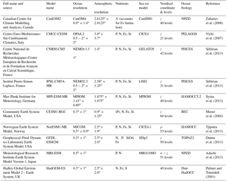
We used 10 models from the Coupled Model Intercomparison Project version 5 (CMIP5) Earth system models (ESM) shown in Table 1. The selection criterion for the models was based on the availability of essential variables for the analysis in the CMIP5 data portal (http://pcmdi9.llnl.gov) at the time of writing: i.e., monthly FCO₂, pCO₂, chlorophyll, net primary production (NPP), surface oxygen, surface dissolved inorganic carbon (DIC), MLD, sea surface temperature (SST), vertical temperature fields and annual DIC for the historical scenario. The analysis is primarily based on the climatology over 1995–2005, which was selected to match a period closest to the available observational data product (Landschützer et al., 2014; 1998–2011). However, we do examine the consistency of the seasonality of FCO₂ over periods longer than 10 years by comparing the seasonal cycle of FCO₂ and temporal standard deviation of 30 years (1975–2005) vs. 10 years (1995–2005) for HadGEM2-ES and CanESM2. We find that the seasonal cycle of FCO₂ remains consistent (R=0.99) in both HadGEM2-ES and CanESM2 over 30 years (Fig. S3). All CMIP5 model outputs were regridded into a common $\mathrm{1}{}^{\circ }\times \mathrm{1}{}^{\circ }$ regular grid throughout the analysis, except for annual CO₂ mean fluxes, which were computed on the original grid for each model.

Table 1 A description of the 10 CMIP5 ESMs that were used in this analysis. It shows the ocean resolution, atmospheric resolution, and available nutrients for the biogeochemical component, sea-ice model, vertical levels and the marine biogeochemical component for each ESM.

2.3 Sea–air CO₂ flux drivers: the seasonal cycle diagnostic framework

The seasonal cycle of the ocean–atmosphere pCO₂ gradient (ΔpCO₂) is the main driver of the variability of FCO₂ over comparable periods (Sarmiento and Gruber, 2006; Wanninkhof et al., 2009; Mongwe et al., 2016). Wind speed plays a dual role as a driver of FCO₂: it drives the seasonal evolution of buoyancy-mixing dynamics, which influences the biogeochemistry and upper water column physics (but these processes are incorporated into the variability of the DIC), as well as the rate of gas exchange across the air–sea interface (Wanninkhof et al., 2013). However, because winds in the Southern Ocean do not have large seasonal variation (Young, 1999), for this analysis we neglect the role of wind as a secondary driver of the seasonal cycle of FCO₂. Consequently, the seasonal cycle of FCO₂ is directly linked to surface pCO₂ variability, influenced by changes in temperature, salinity, TAlk and DIC and macronutrients (Sarmiento and Gruber, 2006; Wanninkhof et al., 2009). In this analysis we use this assumption as a basis to explore how the seasonal variability of temperature and DIC regulate the seasonal cycle of pCO₂ in CMIP5 models relative to observational product estimates.

The seasonal cycle diagnostic framework was developed as a way of scaling the relative contributions from the rates of change of SST- and the total DIC-driven changes to the seasonal cycle of pCO₂ on to a common DIC scale (Mongwe et al., 2016). We use the framework to explore how understanding differences emerging from the temperature- and DIC-driven CO₂ variability could be helpful as a diagnostic of the apparent observation–model seasonal cycle biases in the Southern Ocean.

The total rate of change of DIC in the surface layer consists of the contribution of air–sea exchanges, biological, vertical and horizontal transport-driven changes (Eq. 1).

$$\begin{array}{ll}\text{(1)}& {\displaystyle }& {\displaystyle }{\left({\displaystyle \frac{\partial \text{DIC}}{\partial t}}\right)}_{\text{Tot}}={\left({\displaystyle \frac{\partial \text{DIC}}{\partial t}}\right)}_{\text{air-sea}}+{\left({\displaystyle \frac{\partial \text{DIC}}{\partial t}}\right)}_{\text{Bio}}{\displaystyle }& {\displaystyle }{\left({\displaystyle \frac{\partial \text{DIC}}{\partial t}}\right)}_{\text{Vert}}+{\left({\displaystyle \frac{\partial \text{DIC}}{\partial t}}\right)}_{\text{Hor}}\end{array}$$

Because we used zonal means from medium-resolution models, we assume that the horizontal terms are negligible, though we remain mindful that there could be a seasonal cycle in the divergence of the horizontal transport due to a latitudinal gradient in DIC perturbed by Ekman flow in some regions of the Sub-Antarctic Zone (Rosso et al., 2017). This leaves air–sea exchange, vertical fluxes (advection and diffusion) and biological processes as the dominant drivers of DIC.

Since temperature does not affect DIC changes directly, but only pCO₂ through solubility, it was necessary to scale the influence of temperature into equivalent DIC units in order to compare the influence of temperature vs. DIC control of surface pCO₂ variability. Thus, in order to constrain the contribution of temperature on the seasonal variability of pCO₂ and FCO₂ we derived a new synthetic temperature-linked term “DIC equivalent” (DIC_T) defined as “the magnitude of DIC change that would correspond to a change in pCO₂ driven by a particular temperature change”. In this way the ΔpCO₂ driven solely by modeled or observed temperature change is converted into equivalent DIC units, which allows its contribution to be scaled against the observed or modeled total surface DIC change (Eq. 1). Shifts between temperature and DIC control of pCO₂ are in effect tipping points because they reflect major shifts in the mechanisms that drive pCO₂ variability. We use this as the basis to investigate the possible mechanisms behind model biases in the seasonal cycle of pCO₂.

This calculation of DIC_T is done in two steps: firstly, the temperature impact on pCO₂ is calculated using the Takahashi et al. (1993) empirical expression that linearizes the temperature dependence of the equilibrium constants.

$$\begin{array}{}\text{(2)}& {\left({\displaystyle \frac{\partial p{\mathrm{CO}}_{\mathrm{2}}}{\partial t}}\right)}_{\text{SST}}=p{\mathrm{CO}}_{\mathrm{2}}\times \mathrm{0.0423}\times \left({\displaystyle \frac{\partial \text{SST}}{\partial t}}\right)\end{array}$$

Though this relationship between dSST and dpCO₂ is based on a linear assumption (Takahashi et al., 1993), this formulation has been shown to hold and has been widely used in the literature (e.g., Bakker et al., 2014; Feely et al., 2004; Marinov and Gnanadesikan, 2011; Takahashi et al., 2002; Wanninkhof et al., 2009; Landschützer et al., 2018). We show in the Supplement that the extension of this expression into polar temperature ranges (SST < 2 ^∘C) only introduces a minor additional uncertainty of 4–5 % (SM Fig. S4).

Secondly, the temperature-driven change in pCO₂ is converted to an equivalent DIC_T using the Revelle factor.

$$\begin{array}{}\text{(3)}& {\left({\displaystyle \frac{\partial {\text{DIC}}_T}{\partial t}}\right)}_{\text{SST}}={\displaystyle \frac{\text{DIC}}{{\mathit{\gamma }}_{\text{DIC}}\times p{\mathrm{CO}}_{\mathrm{2}}}}{\left({\displaystyle \frac{\partial p{\mathrm{CO}}_{\mathrm{2}}}{\partial t}}\right)}_{\text{SST}}\end{array}$$

Here we also used a fixed value for the Revelle factor (γ_DIC=14), typical of polar waters in the Southern Ocean in order to assess the error linked to this assumption. We recomputed the Revelle factor in the Sub-Antarctic and Antarctic zones using annual mean climatologies of TAlk, salinity, sea surface temperature and nutrients. Firstly, we examined DIC changes for the nominal range of pCO₂ change (340–399 µatm :1 µatm intervals) and then used this dataset to derive the Revelle factor. The range of calculated Revelle factors in the Southern Ocean was between γ_DIC ∼ 12 and 15.5 with an average of γ_DIC=13.9 ± 1.3. This justifies our use of γ_DIC=14 for the conversion of the solubility-driven pCO₂ change to an equivalent DIC (DICT) throughout the analysis. We have provided the uncertainty that this conversion makes into the temperature constraint DIC_T by using the upper and lower limits of the Revelle factor (${\mathit{\gamma }}_{\text{DIC}}=\mathrm{12}-\mathrm{15.5}$) in the model framework. In the Supplement (Fig. S5) we show examples for observations in the Sub-Antarctic and Antarctic zones, which indicate that the extremes of the Revelle factor values (${\mathit{\gamma }}_{\text{DIC}}=\mathrm{12}-\mathrm{15.5}$) do not alter the phasing or magnitude of the relative controls of temperature or DIC on the seasonal cycle of pCO₂.

The rate of change of DIC was discretized on a monthly mean as follows:

$$\begin{array}{}\text{(4)}& {\left({\displaystyle \frac{\partial {\text{DIC}}_T}{\partial t}}\right)}_{\text{SST}}\approx {\left({\displaystyle \frac{\mathrm{\Delta }\text{DIC}}{\mathrm{\Delta }t}}\right)}_{n,l}={\displaystyle \frac{{\text{DIC}}_{n+\mathrm{1},l}-{\text{DIC}}_{n,l}}{\mathrm{1}\text{ month}}},\end{array}$$

where n is time in month, l is vertical level (in this case the surface, l=1). We here take the forward derivative such that November rate is the difference between 15 November and 15 December, thus being centered at the interval between the months.

Finally, to characterize periods of temperature or DIC dominance as main drivers of the instantaneous (monthly) pCO₂ change we subtract Eq. (1) from Eq. (4), which yields a residual indicator M_T-DIC Eq. (5). M_T-DIC is then used as indicator of the dominant driver of instantaneous pCO₂ changes in this scale monthly timescale.

$$\begin{array}{}\text{(5)}& M_{T\text{-DIC}}=\left|{\left({\displaystyle \frac{\partial {\text{DIC}}_T}{\partial t}}\right)}_{\text{SST}}\right|-\left|{\left({\displaystyle \frac{\partial \text{DIC}}{\partial t}}\right)}_{\text{Tot}}\right|\end{array}$$

M_T-DIC>0 indicates that the pCO₂ variability is dominated by the temperature-driven solubility and when M_T-DIC<0, it indicates that pCO₂ changes are mainly modulated by DIC processes (i.e., biological CO₂ changes and vertical-scale physical DIC mechanisms). We also examine the following DIC processes: (i) biological DIC changes using chlorophyll, NPP, export carbon, and surface oxygen and (ii) physical DIC mechanisms using estimated entrainment rates at the base of the mixed layer. Details of this calculation are in Sect. 2.4.

In the Southern Ocean, salinity and TAlk are considered lower-order drivers of the seasonal cycle of pCO₂ (Takahashi et al., 1993). In the Supplement (Fig. S6), we show that salinity and TAlk do not play a major role as drivers of the local seasonal cycle of pCO₂. We do so by computing the equivalent rate of change of DIC resulting from seasonal variability of salinity and TAlk as done for temperature (Eq. 2), i.e., still assuming empirical linear relationships from Takahashi et al. (1993): $\left(\frac{\ln \left(p{\text{CO}}_{\mathrm{2}}\right)}{\ln \left(\text{TAlk}\right)}\approx -\mathrm{9.4}\right)$ and $\left(\frac{\ln \left(p{\text{CO}}_{\mathrm{2}}\right)}{\ln \left(\text{Sal}\right)}=\mathrm{0.94}\right)$. By applying these relationships to the model data, we confirmed that salinity and TAlk are indeed secondary drivers of pCO₂ changes, i.e., ${\left[{\left(\frac{\partial \text{DIC}}{\partial t}\right)}_{\text{Tot}}\right]}_{\text{average}}$. ≈5 µmol kg⁻¹ month⁻¹, while ${\left[{\left(\frac{\partial \text{DIC}}{\partial t}\right)}_{\text{Tot}}\right]}_{\text{average}}\approx \mathrm{0.6}$ µmol kg⁻¹ month⁻¹ and ${\left[{\left(\frac{\partial \text{DIC}}{\partial t}\right)}_{\text{TAlk}}\right]}_{\text{maximum}}\approx \mathrm{0.4}$ µmol kg⁻¹ month⁻¹.

2.4 Entrainment mixing

CO₂ uptake by the Southern Ocean has been shown to weaken during winter linked to the entrainment of sub-surface DIC as the MLD deepens (e.g., Lenton et al., 2013; Metzl et al., 2006; Takahashi et al., 2009). Here we estimate this rate of entrainment (RE) using Eq. (6), which estimates the advection of preformed DIC at the base of the mixed layer:

$$\begin{array}{}\text{(6)}& {\displaystyle }& {\displaystyle }\text{RE}=U_{\text{e}}{\left({\displaystyle \frac{\partial \text{DIC}}{\partial z}}\right)}_{\text{MLD}},\text{(7)}& {\displaystyle }& {\displaystyle }{\text{RE}}_n=\left({\displaystyle \frac{\mathrm{\Delta }{\text{MLD}}_n}{\mathrm{\Delta }t}}\right){\left({\displaystyle \frac{\mathrm{\Delta }\text{DIC}}{\mathrm{\Delta }z}}\right)}_{n,\text{ MLD}},\text{(8)}& {\displaystyle }& {\displaystyle }{\left({\displaystyle \frac{\mathrm{\Delta }\text{DIC}}{\mathrm{\Delta }z}}\right)}_{n,\text{MLD}}={\displaystyle \frac{{\text{DIC}}_{n,{\text{MLD}}_{n+\mathrm{1}}}-{\text{DIC}}_{n,{\text{MLD}}_n}}{\mathrm{\Delta }z}},\end{array}$$

in which U_e is an equivalent entrainment velocity based on the rate of change of the MLD and n is the time in months. This approximation of vertical entrainment is necessary as it is not possible to compute this term from the CMIP5 data because the vertical DIC distribution is only available as an annual means. We use the entrainment rates to estimate the influence of subsurface/bottom DIC changes on surface DIC changes and subsequently pCO₂ and FCO₂. Because we are mainly interested in the period autumn–winter, where the MLD ≥ 60 m in the Sub-Antarctic Zone and ≥ 40 m in the Antarctic Zone at this depth seasonal variations in DIC are anticipated to be minimal – these estimates can be used. The monthly and annual mean DIC from a NEMO PISCES 0.5 × 0.5^∘ model output were used to estimate the uncertainty by comparing RE computed from both (Dufour et al., 2013). We found the annual and monthly estimates to be indeed comparable with minimal differences (not shown). It is noted as a caveat that this rate of entrainment is only a coarse estimate because we were using annual means and is intended only for the autumn–winter period, when MLDs are deepened.

Figure 1 The annual mean climatological distribution sea–air CO₂ flux (FCO₂, in gC m⁻² yr⁻¹) for observations (L14: Landschützer et al., 2014; T09: Takahashi et al., 2009) and 10 CMIP5 models over 1995–2005. CMIP5 models broadly capture the spatial distribution of FCO₂ with respect to L14 and T09; however, they also show significant differences in space and magnitude between the basins of the Southern Ocean, with a few exceptions.

3 Results

3.1 Annual climatological sea–air CO₂ fluxes

The annual mean climatological distribution of FCO₂ in the Southern Ocean obtained from observational products is spatially variable, but mainly characterized by two key features: (i) CO₂ in-gassing north of 50–55^∘ S (Polar Frontal Zone, PFZ) within and north of the Sub-Antarctic Zone, and (ii) CO₂ out-gassing between the PF (∼ 58^∘ S) and the marginal ice zone (MIZ, ∼ 60–68^∘ S) (Fig. 1a–b). Most CMIP5 models broadly capture these features; however, they also show significant differences in space and magnitude between the basins of the Southern Ocean (Fig. 1). With the exception of CMCC-CESM, which shows a northerly extended CO₂ out-gassing band between about 40 and 50^∘ S, CMIP5 models generally show the CO₂ out-gassing zone between 50 and 70^∘ S, in agreement with observational estimates (Fig. 1).

The analyzed 10 CMIP5 models show a large spatial dispersion in the spatial representation of the magnitudes of FCO₂ with respect to observations (Fig. 1, Table  2). They generally overestimate the upwelling-driven CO₂ out-gassing (55–70^∘ S) in some basins relative to observations. IPSL-CM5A, CanESM2, MPI-ESM, GFDL-ESM2M and MRI-ESM, for example, show CO₂ out-gassing fluxes reaching up to 25 g m⁻² yr⁻¹, while observations only show a maximum of 8 g m⁻² yr⁻¹ (Fig. 1). Between 40 and 56^∘ S (Sub-Antarctic Zone), observations and CMIP5 models largely agree, showing a CO₂ in-gassing feature, which is mainly attributable to biological processes (McNeil et al., 2007; Takahashi et al., 2012). South of 65^∘ S, in the MIZ, models generally show an excessive CO₂ in-gassing with respect to observations (with the exception of CanESM2, IPSL-CM5A-MR and CNRM-CM5). Note that as much as this bias south of the MIZ might be a true divergence of CMIP5 models from the observed ocean, it is also possibly due to the lack of observations in this region, especially during the winter season (Bakker et al., 2014; Monteiro, 2010).

Table 2 shows the pattern correlation coefficient (PCC) and the Root mean square error (RMSE), which are here used to quantify the model spatial and magnitude performances against Landschützer et al. (2014) data product. Out of the 10 models, 6 show a moderate spatial correlation with Landschützer et al. (2014) (PCC = 0.40–0.60), i.e., CNRM-CM5, GFDL-ESM2M, HadGEM2-ES, IPSL-CM5A-MR, CESM1-BGC, NorESME-ME and CanESM2. While MPI-ESM-MR (PCC = 0.37), MRI-ESM (PCC = 0.36) and CMCC-CESM (PCC = −0.09) show a weak to null spatial correlation with observations, the last of these is mainly due to the overestimated out-gassing region. Spatially, GFDL-ESM2M and NorESM1-ME are the most comparable to Landschützer et al. (2014), (RMSE < 9), while CCMC-CESM, CanESM2, MRI-ESM and CNRM-CM5 shows the most differences (REMSE > 15). The rest of the models show a modest comparison (RSME 9–11).

NorESM1-ME and CESM1-BGC are the only 2 of the 10 models showing a consistent spatial (REMSE < 9) and magnitude (PCC ≈ 0.50) performance. From Table 2, it is evident that an appropriate representation of the spatial properties of FCO₂ with respect to observations does not always correspond to comparable magnitudes. CanESM2, for example, shows a good spatial comparison (PCC = 0.54), yet a poor estimation of the magnitudes (RMSE = 19.5). In this case this is caused by an overestimation of CO₂ uptake north of 55^∘ S (≈ −28 g m⁻² yr⁻¹) and CO₂ out-gassing (> 25 g m⁻² yr⁻¹) in the Antarctic Zone, resulting in a net total Southern Ocean annual weak sink (−0.05 Pg C m⁻² yr⁻¹).

3.2 Sea–air CO₂ flux seasonal cycle variability and biases

The seasonal cycle of FCO₂ is shown in Fig. 2. The seasonality of FCO₂ in the 10 CMIP5 models shows a large dispersion in both phasing and amplitude but mostly disagrees with observations in the phase of the seasonal cycle, and the models mostly disagree among each other. More quantitatively, CMIP5 models show weak to negative correlations with the Landschützer et al. (2014) data product in the Sub-Antarctic Zone and have slightly higher correlations in the Antarctic Zone (see Supplement Fig. S7). This discrepancy is consistent with the findings of Anav et al. (2013), who, however, used fixed latitude criteria. Based on the phasing, the seasonality of FCO₂ in CMIP5 models can be a priori divided into two main groups: (1) group-DIC models, comprising MPI-ESM, HadGEM-ES and NorESM1-ME, and group-SST models, and (2) the remainder, i.e., GFDL-ESM2M, CMCC-CESM, CNRM-CERFACS, IPSL-CM5A-MR, CESM1-BGC, MRI-ESM and CanESM2. The naming convention is suggestive of the mechanism driving the seasonal cycle, as will be clarified further on. A similar grouping was also identified by Kessler and Tjiputra (2016) using a different criterion. Figure 3 shows the seasonal cycle of FCO₂ of an equally weighted ensemble of the two groups compared to observations; the shaded area shows the decadal standard deviation for the models and the Landschützer et al. (2014) data product for 1998–2014 standard deviation in the various regions.

Figure 2 Seasonal cycle of sea–air CO₂ flux (FCO₂, in gC m⁻² yr⁻¹) in observations and 10 CMIP5 models in the Sub-Antarctic and Antarctic zones of the Pacific Ocean (first column), Atlantic Ocean (second column) and Indian Ocean (third column). The shaded area shows the temporal standard deviation over the considered period (1995–2005).

In the Sub-Antarctic Zone, the observational products show a weakening of CO₂ uptake during winter (less negative values in June–August) with values close to the zero at the onset of spring (September) in all three basins. Similarly, during the spring season, all three basins are seen to maintain a steady increase in CO₂ uptake until mid-summer (December), while they differ during autumn (March–May). The Pacific Basin shows an increase in CO₂ uptake during autumn that is not observed in the other basins (only marginally in the Indian zone). In the Antarctic Zone, the observed FCO₂ seasonal cycle is mostly similar in all three basins (Fig. 3d–f). While this seasonal cycle consistency may suggest a spatial uniformity of the mechanisms of FCO₂ at the Antarctic, we are also mindful that this may be due to a result of the paucity of observations in this area. In the Antarctic Zone, all three basins show a weakening of uptake or increasing of out-gassing from the onset of autumn (March) until mid-winter (June–July). The winter CO₂ out-gassing is followed by a strengthening of the CO₂ uptake throughout spring to summer, when it reaches a CO₂ in-gassing peak.

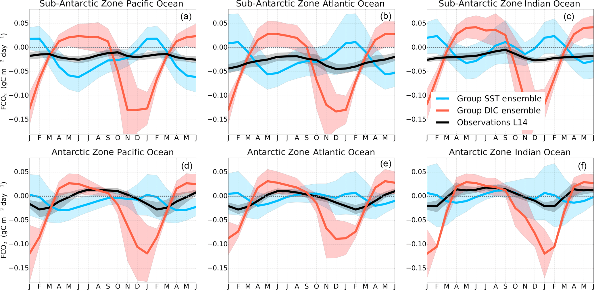
Figure 3 Seasonal cycle of the equally weighted ensemble means of FCO₂ (gC m⁻² yr⁻¹) from Fig. 2 for group DIC models (MPI-ESM, HadGEM-ES and NorESM) and group SST models (GFDL-ESM2M, CMCC-CESM, CNRM-CERFACS, IPSL-CM5A-MR, CESM1-BGC, NorESM2, MRI-ESM and CanESM2). The shaded areas show the ensemble standard deviation. The black line is the Landschützer et al. (2014) observations.

The differences in the seasonal cycle of FCO₂ across the three basins of the Sub-Antarctic Zone found in the observational product (Fig. 2) are likely a consequence of spatial differences seen in Fig. 1. To verify this, we calculated the correlation between the seasonal cycles from the Landschützer et al. (2014) observational product in the three basins (Fig. 4). The FCO₂ seasonal cycle in the Sub-Antarctic Atlantic and Indian basins are similar (R=0.8), while the other basins are quite different to one another ($R=-\mathrm{0.1}$ for Pacific–Atlantic and R ∼ 0.4 for Pacific–Indian). Contrary to the observational product, CMIP5 models show the same seasonal cycle phasing across all three basins in the Sub-Antarctic Zone (basin–basin correlation coefficients are always larger than 0.50 in Fig. 4 despite the spatial differences in Fig. 2, with the exception of three models, i.e., CMCC-CESM, CESM-BGC1 and GFDL-ESM2M). Thus, contrary to Landschützer et al. (2014), CMIP5 models shows a zonal homogeneity in the seasonal cycle of FCO₂, which may suggest that the drivers of CO₂ are less regional. In the Antarctic Zone, CMIP5 models agree with observations in the spatial uniformity of the seasonal cycle of FCO₂ across the three basins.

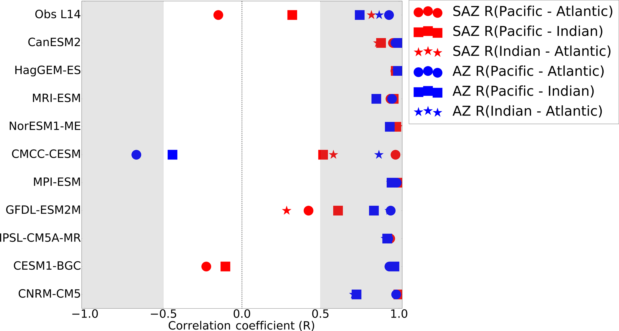
Figure 4 The correlation coefficients (R) of basin–basin seasonal cycles of FCO₂ for observations (Landschützer et al., 2014) and 10 CMIP5 models in the three basins of the Southern Ocean, i.e., Pacific, Atlantic and Indian basins.

Group-DIC models are characterized by an exaggerated CO₂ uptake during spring–summer (Fig. 3) with respect to observation estimates and CO₂ out-gassing during winter. These models generally agree with observations in the phasing of CO₂ uptake during spring, but overestimate the magnitudes. It is worth noting that the seasonal characteristics of group-DIC models are mostly in agreement with the observations in the Atlantic and Indian basins in Sub-Antarctic Zone (R>0.5 in Fig. 4). The large standard deviation (∼ 0.01 g C m⁻² day⁻¹) during the winter and spring–summer seasons in the Atlantic Basin shows that though group-DIC models agree in the phase, magnitudes vary considerably (Fig. 3b). For example MPI-ESM reaches up to 0.06 g C m⁻² day⁻¹out-gassing during winter, while HadESM2-ES and NorESM2 peak only at ∼ 0.03 g C m⁻² day⁻¹. Group-SST models on the other hand are characterized by a CO₂ out-gassing peak in summer (December–February) and a CO₂ in-gassing peak at the end of autumn (May), and their phase is opposite to the observational estimates in the Atlantic and Indian basins (Fig. 3b, c). Group-SST models only show a strengthening of CO₂ uptake during spring in the Indian Basin. Interestingly, group-SST models compare relatively well with the observed FCO₂ seasonal cycle in the Pacific Basin, whereas group-DIC models disagree the most with the observed estimates (Fig. 3a). This phasing difference within models and against observed estimates probably suggests that the disagreement of CMIP5 models FCO₂ with observations is not a matter of a relative error/constant magnitude offset but most likely points to differences in the seasonal drivers of FCO₂.

In the Antarctic Zone (Fig. 3d–f), both group-DIC and group-SST models perform better than in the Sub-Antarctic, with respect to phasing and amplitude in as shown by the correlation analysis in Fig. S7. Models reflect comparable pCO₂ seasonality in the different basins of the AZ to the observational products (Fig. 4, with the exception of MRI-ESM and CanESM2, where R<0 for all three basins). Here FCO₂ magnitudes oscillate around zero with the largest disagreements occurring during mid-summer, where observation estimates show a weak CO₂ sink ($\approx -\mathrm{0.03}$ gC m⁻² day⁻¹), and group-SST show a zero net CO₂ flux and a strong uptake in group DIC (e.g., $\approx -\mathrm{0.12}$ gC m⁻² day⁻¹ in the Pacific Basin). The large standard deviation (≈0.01 gC m⁻² day⁻¹) here indicates considerable differences among models (Fig. 3d–f).

Figure 5 Mean seasonal cycle of the estimated rate of change of sea-surface temperature (dSST ∕ dt, ^∘C month⁻¹) for the Sub-Antarctic and Antarctic zones of the Pacific Ocean (first column), Atlantic Ocean (second column) and Indian Ocean (third column).

3.3 Seasonal-scale drivers of sea–air CO₂ flux

We now examine how changes in temperature and DIC regulate FCO₂ variability at the seasonal scale following the method described in Sect. 2.3. Figure 5 shows the monthly rates of change of SST (dSST ∕ dt) for the 10 models compared with WOA13 SST. CMIP5 generally shows agreement in the timing of the switch from surface cooling (dSST ∕ dt<0) to warming (dSST ∕ dt>0) and vice versa, i.e., March (summer to autumn) and September (winter to spring), respectively. In both the Sub-Antarctic and Antarctic Zone CMIP5 models agree with observations in this timing (Fig. 5). However, while they agree in phasing, the amplitude of these warming and cooling rates are overestimated with respect to the WOA13 dataset with the exception of NorESM1-ME. Subsequently these differences in the magnitude of dSST ∕ dt have important implications for the solubility of CO₂ in seawater, with larger magnitudes of |dSST∕dt| likely to enhance the response of the pCO₂ to temperature through CO₂ solubility changes. For example, because the observations in the Indian Basin show a warming rate of about 0.5 ^∘C month⁻¹ lower compared to the other two basins, we expect a relatively weaker role of surface temperature in this basin.

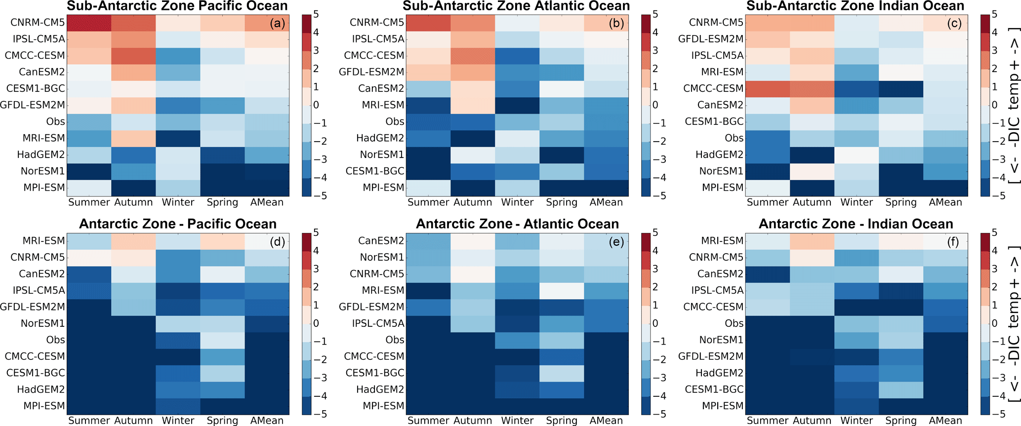
Figure 6 Mean seasonal and annual values of the DIC–temperature control index (M_T-DIC). The increase in the red color intensity indicates increase in the strength of the temperature driver and the blue intensity shows the strength of the DIC driver. The models are sorted according to the annual mean value of the indicator presented in the last column (AMean).

As described in Sect. 2.3, the computed dSSt/dt magnitudes were used to estimate the equivalent rate of change of DIC driven by CO₂ solubility using Eq. (2). The seasonal cycle of |(dDIC_T∕dt)_SST| vs. |(dDIC∕dt)_Tot|, for the 10 models and observations is presented in the Supplement (Fig. S8), where we show the seasonal mean of M_T-DIC from (Eq. 3). As articulated in Sect. 2.3, M_T-DIC (Fig. 6) is the difference between the total surface DIC rate of change of DIC (Eq. 1) and the estimated equivalent temperature-driven solubility DIC changes Eq. (3), such that when |(dDIC_T∕dt)_SST| > |(dDIC∕dt)_Tot|, temperature is the dominant driver of the instantaneous pCO₂ changes, and conversely when |(dDIC_T∕dt)_SST| < |(dDIC∕dt)_Tot|, DIC processes are the dominant mode in the instantaneous pCO₂ variability. The models showing the former feature are SST-driven and belong to group-SST, while the models showing the latter are DIC-driven and belong to group-SST.

According to the M_T-DIC magnitudes in Fig. 6, the seasonal cycle of pCO₂ in the observational estimates is predominantly DIC-driven most of the year in both the Sub-Antarctic and Antarctic Zone. Note that, however, during periods of high |dSST∕dt|, i.e., autumn and spring, observations show a moderate to weak DIC control (M_T-DIC≈0). The Antarctic Zone is mostly characterized by a stronger DIC control (mean annual M_T-DIC>0) except for during the spring season (Fig. 6). Consistent with the similarity analysis presented in Fig. 4, the Antarctic Zone shows coherence in the sign of the temperature–DIC indicator (M_T-DIC>0) within the three basins.

3.4 Source terms in the DIC surface budget

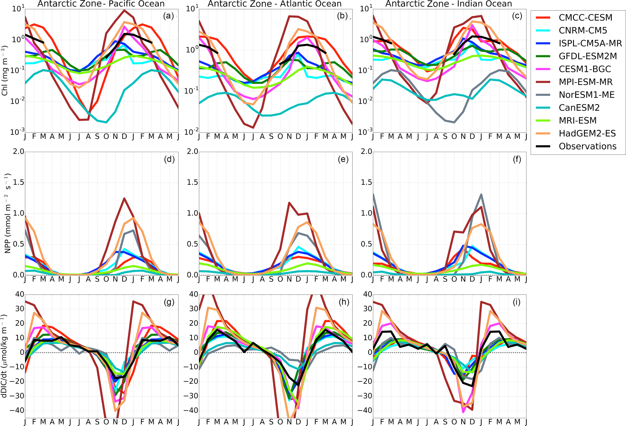
To further constrain the surface DIC budget in Eq. (1), we examine the role of the biological source term using chlorophyll and net primary production (NPP) as proxies. Figure 8 shows the seasonal cycle of chlorophyll, NPP and the rate of surface DIC changes (dDIC ∕ dt). The observed seasonal cycle of chlorophyll (Johnson et al., 2013) shows a similar seasonal cycle within the three basins during the spring–summer seasons (autumn–winter data are removed due to the satellite limitation) in both the Sub-Antarctic and Antarctic Zone. Magnitudes are, however, different in the Sub-Antarctic Zone; the Atlantic Basin shows larger chlorophyll magnitudes (chlorophyll reach up to 1.0 mg m⁻³) compared to the Pacific and Indian basins (Chl < 1 mg m⁻³).

CMIP5 models here show a clear partition between group-DIC and group-SST models. While they mostly maintain the same phase, group-DIC shows larger amplitudes of chlorophyll relative to group-SST and observed estimates in the Sub-Antarctic Zone. This difference is even clearer in NPP magnitudes, where group-DIC models show a maximum of NPP > 1 mmol m⁻² s⁻¹ in summer, while group-SST magnitudes shows about half of it. Except for CESM1-BGC and CMCC-CESM (and NorESM1-ME for NPP), each CMIP5 model generally maintains a similar chlorophyll seasonal cycle (phase and magnitude) in all three basins of the Southern Ocean. This is contrary to the observations, which show differences in the magnitude. Consistent with the observational product, CESM1-BGC simulates larger amplitude in the Atlantic Basin. While CMCC-CESM also has this feature, it also shows an overestimated chlorophyll peak in the Indian Basin. In the Antarctic Zone both observations and CMIP5 models generally agree in both phase and magnitude (except for CanESM2) of the seasonal cycle of chlorophyll in all three basins.

Figure 7 Seasonal cycle of the mixed layer depth (MLD) in the Sub-Antarctic and Antarctic zones of the Pacific Ocean (first column), Atlantic Ocean (second column) and Indian Ocean (third column).

We now examine the influence of the vertical DIC rate in Eq. (1), using estimated entrainment rates (RE, Eq. 5) based on MLD and vertical DIC gradients (see Sect. 2.3). Figure 7 shows the seasonal changes of MLD compared with the rate from the observational product. CMIP5 models largely agree on the timing of the onset of MLD deepening (February in the Pacific Basin, and March for the Atlantic and Indian basins) and shoaling (September) in the Sub-Antarctic Zone (with the exception of NorESM1-ME and IPSL-CM5A in the Pacific Basin). The Indian Basin generally shows deeper winter MLD in both observations and CMIP5 models in the Sub-Antarctic Zone. Note that while CMIP5 models generally show the observed deeper MLDs in the Indian Basin, they show a large variation; for example, the winter maximum depth ranges from 100 m (CMCC-CESM, Pacific Basin) to 350 m (CanESM2, Indian Basin) in the Sub-Antarctic Zone. In the Antarctic Zone CMIP5 models are largely in agreement on the timing of the onset of MLD deepening (February) but also variable in their winter maximum depth. It is worth noting that the observed MLD seasonal cycle might be biased due to limited in situ observations particularly in the Antarctic Zone (de Boyer Montégut et al., 2004).

The estimated RE values in Fig. 10 show that almost all CMIP5 models (with the exception of NorESM1-ME) entrain subsurface DIC into the mixed layer during autumn–winter, in agreement with the observational estimates. In the Sub-Antarctic Zone, the estimates using the observational products show the strongest entrainment in the Atlantic Basin in May (RE reaches up to 10 µmol kg⁻¹ month⁻¹), while it is lower in the other basins. In the Antarctic Zone, observed RE conversely shows stronger entrainment rates in the Pacific and Indian basins (RE > 15 µmol kg⁻¹ month⁻¹) in comparison to the Atlantic Basin (RE = 11 µmol kg⁻¹ month⁻¹). CMIP5 models entrainment rates are variable but not showing any particular deficiency when compared with the observational estimates. Also, the group-DIC and group-SST models show no clear distinction, the major striking features being the relatively stronger entrainment in MPI-ESM and CanESM2 across the three basins in the Sub-Antarctic Zone in mid- to late winter (RE = 15 µmol kg⁻¹ month⁻¹), and the large winter entrainment in IPSL-CM5A-MR in the Antarctic Pacific Basin. The supply of DIC to the surface due to vertical entrainment is therefore generally comparable between model simulations and the available estimate.

However, our RE estimates are estimated at the base of the mixed layer, which is not necessarily a complete measure of the vertical flux of DIC at the surface. We therefore investigate the annual mean vertical DIC gradients in Fig. 10 as an indicator of where the surface uptake processes occur. The simulated CMIP5 profiles are similar to GLODAP2, but some differences arise. In the Sub-Antarctic Zone, GLODAP2 shows a shallower surface maximum in the Atlantic Basin consistent with higher biomass in this basin (Fig. 8) ((dDIC ∕dz)_smax=0.55 µmol kg⁻¹ m⁻¹, at 50 m) compared to the Pacific ((dDIC ∕ dz)_smax=0.60 µmol kg⁻¹ m⁻¹, at 80 m) and Indian Basin ((dDIC ∕ dz)_smax=0.40 µmol kg⁻¹ m⁻¹, at 80 m). CMIP5 models generally do not show this feature in the Sub-Antarctic Zone, except for CESM1-BGC1 ((dDIC ∕ dz)_smax=0.50 µmol kg⁻¹ m⁻¹, at 50 m). Instead, they show the surface maxima at the same depth in all three basins. In the Antarctic Zone both CMIP5 models and observations show larger (dDIC ∕ dz)_smax magnitudes and nearer surface maxima (with the exception of CanESM2 and CESM1-BGC). This difference in the position and magnitude of the DIC maxima between the Sub-Antarctic and Antarctic Zone has important implications for surface DIC changes and subsequently pCO₂ seasonal variability. Because of the nearer surface DIC maxima in the Antarctic Zone, surface DIC changes are mostly influenced by these strong near-surface vertical gradients compared to MLD changes. This implies that even if the entrainment rates at the base of the MLD are comparable between the Sub-Antarctic and the Antarctic, the surface supply of DIC may be larger in the Antarctic Zone.

4 Discussion

Recent studies have highlighted that important differences exist between the seasonal cycle of pCO₂ in models and observations in the Southern Ocean (Lenton et al., 2013; Anav et al., 2015; Mongwe, 2016). Paradoxically, although the models may be in relative agreement for the mean annual flux, they diverge in the phasing and magnitude of the seasonal cycle (Lenton et al., 2013; Anav et al., 2015; Mongwe, 2016). These differences in the seasonal cycle raise questions about the climate sensitivity of the carbon cycle in these models because they may reflect differences in the process sensitivities to drivers that are themselves climate sensitive.

In this study we expand on the framework proposed by Mongwe et al. (2016), which examined the competing roles of temperature and DIC as drivers of pCO₂ variability and the seasonal cycle of pCO₂ in the Southern Ocean, to explain the mechanistic basis for seasonal biases of pCO₂ and FCO₂ between observational products and CMIP5 models. This analysis of 10 CMIP5 models and one observational product (Landschützer et al., 2014) highlighted that although the models showed different seasonal cycles (Fig. 2), they could be grouped into two categories (SST- and DIC-driven) according to their mean seasonal bias of temperature or DIC control (Figs. 3, 6).

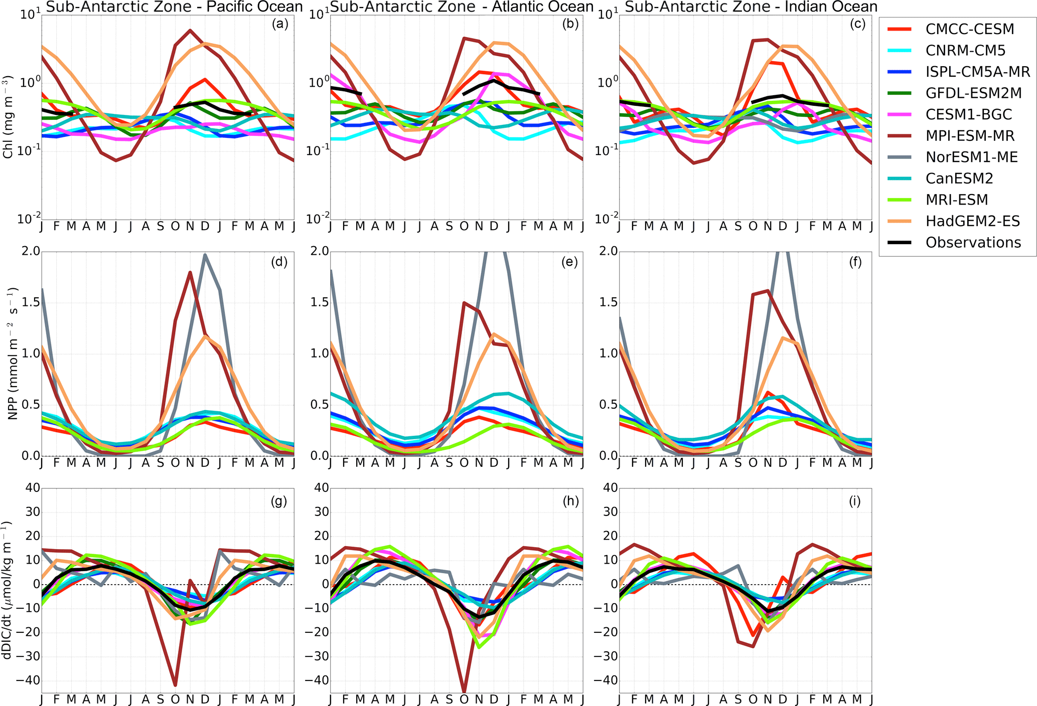
Figure 8 The seasonal cycle of chlorophyll (mg m⁻³), net primary production (mmol m⁻² s⁻¹) and the surface rate of change of DIC (µmol kg⁻¹ month⁻¹) in the Sub-Antarctic Zone of the Pacific Ocean (first column), Atlantic Ocean (second column) and Indian Ocean (third column).

A few general insights emerge from this analysis. Firstly, despite significant differences in the spatial characteristics of the mean annual fluxes (Fig. 1), models show unexpectedly greater inter-basin coherence in the phasing seasonal cycle of FCO₂ and SST-DIC control than observational products (Fig. 3, 6). Clear inter-basin differences have been highlighted in studies on the climatology and interannual variability that examined pCO₂ and CO₂ fluxes based on data products (Landschützer et al., 2015; Gregor et al., 2017), as well as phytoplankton chlorophyll based on remote sensing (Thomalla et al., 2011; Carranza et al., 2016). Briefly, the Atlantic Basin shows the highest mean primary production in contrast to the Pacific Basin, which has the lowest (Thomalla et al., 2011). Similarly, strong inter-basin differences for pCO₂ and FCO₂ have been highlighted and ascribed to SST control (Landschützer et al., 2016) and wind stress–mixed layer depth (Gregor et al., 2017). The combined effect of these regional differences in forcing of pCO₂ and FCO₂ would be expected to be reflected in the CMIP5 models as well. A quantitative analysis of the correlation of the phasing of the seasonal cycle of FCO₂ between basins for different models shows that all the models except three (CMCC-CESM, GFDL-ESM2M, CESM1-CESM) are characterized by strong inter-basin correlation in both the Sub-Antarctic and Antarctic zones (Fig. 4). This suggests that the carbon cycle in these CMIP5 models is not sensitive to inter-basin differences in the drivers as is the case for observations. This most likely implies that CMIP5 models are not sensitive to regional FCO₂ variability at the basin scale, so FCO₂ seasonal biases are zonally uniform.

Secondly, an important part of this analysis is based on the assumption that the observational products that are used to constrain the spatial and temporal variability of pCO₂ and FCO₂ reflect the correct seasonal cycles of the Southern Ocean. This assumption requires significant caution not only due to the limitations in the sparseness of the in situ observations but also due to limitations of the empirical techniques in overcoming these data gaps (Landschützer et al., 2014; Rödenbeck et al., 2015; Gregor et al., 2017, 2018; Ritter et al., 2017). The uncertainty analysis from these studies suggests that, while the seasonal bias in observations may be less in the Sub-Antarctic Zone and PFZ, it is the highest in the AZ, where access is limited mostly to summer and winter ice cover results in uncertainties that may limit the significance of the data–model comparisons. It is important to note that though the observation product that we use here (Landschützer et al. (2014) is based on more surface measurement (10 million, SOCAT v3) compared to previous datasets (e.g., Tahakahashi et al., 2009, 3 million), the data are still sparse in time and space in the Southern Ocean. Thus, in using this data product as our main observational estimates for this analysis we are mindful of the limitations in the discussion below.

Thirdly, the seasonal cycle of ΔpCO₂ is the dominant mode of variability in FCO₂ (Mongwe et al., 2016; Wanninkhof et al., 2009). Though winds provide the kinematic forcing for air–sea fluxes of CO₂ and indirectly affect FCO₂ through mixed layer dynamics and associated biogeochemical responses (Mahadevan et al., 2012; du Plessis et al., 2017), ΔpCO₂ sets the direction of the flux. Surface pCO₂ changes are mainly driven by DIC and SST (Hauck et al., 2015; Takahashi et al., 1993). Subsequently the sensitivity of CMIP5 models to how changes in DIC and SST regulate the seasonal cycle of FCO₂ is fundamental to the model's ability to resolve the observed FCO₂ seasonal cycle. Thus, here we examined the influence of DIC and SST on FCO₂ at seasonal scale for 10 CMIP5 models with respect to observed estimates. Because temperature does not directly affect DIC changes, we first scaled up the impact of SST changes on pCO₂ through surface CO₂ solubility to equivalent DIC units using the Revelle factor (Sect. 2.3). In this way, we can distinguish the influence of surface solubility and DIC changes (i.e., biological and physical) on pCO₂ and hence on FCO₂.

Fourthly, using this analysis framework (Sect. 2.3, summarized in Fig. 6) we found that CMIP5 models FCO₂ biases cluster in two groups, namely group-DIC (M_T-DIC<0) and group-SST (M_T-DIC>0). Group-DIC models are characterized by an overestimation of the influence of DIC on pCO₂ with respect to observations estimates, which instead indicate that physical and biogeochemical changes in the DIC concentration mostly regulate the seasonal cycle of FCO₂ (in short, DIC control). Group-SST models show an excessive temperature influence on pCO₂; here surface CO₂ solubility biases are mainly responsible for the departure of modeled FCO₂ from the observational products. While CMIP5 models mostly show a singular dominant influence of these extremes, observations show a modest influence of both, with a dominance of DIC changes as the main driver of seasonal FCO₂ variability. Below we discuss the seasonal cycle characteristics and possible mechanisms for these two groups of CMIP5 models in the Sub-Antarctic and Antarctic zones of the Southern Ocean.

4.1 Sub-Antarctic Zone (SAZ)

Our diagnostic analysis indicates that the seasonal cycle of pCO₂ in the observational product (Landschützer et al., 2014) is mostly DIC controlled across all three basins of the SAZ (M_T-DIC<0 in Fig. 6). The Atlantic Basin shows a stronger DIC control (annual mean M_T-DIC≥2) compared to the Pacific and Indian basins (annual mean M_T-DIC≈1). This stronger influence of DIC on pCO₂ in the Atlantic Basin is consistent with higher primary production in this basin (Graham et al., 2015; Thomalla et al., 2011), here shown by the larger mean seasonal chlorophyll from remote sensing in the Atlantic Basin with respect to the Pacific and Indian basins (Fig. 8). This significant basin difference is most likely linked to the fact that the Atlantic Basin has longer periods of shallow MLD compared to the Pacific and Indian basins (Fig. 7a–c, November–March and November–February, respectively) and has been shown to have higher supplies of continental shelves and land-based iron (Boyd and Ellwood, 2010; Tagliabue et al., 2012, 2014). These conditions are more likely to enhance primary production that translates into a higher rate of change of surface DIC (Fig. 8), which becomes the major driver of FCO₂ variability. In contrast, shorter periods of shallow MLD and lower iron inputs in the Pacific Basin (Tagliabue et al., 2012) likely account for a lower chlorophyll biomass and hence the weaker DIC control evidenced in our analysis ($M_{T\text{-DIC}}=\approx \mathrm{0}$ in Fig. 6). In the Indian Basin, the winter mixed layer is deeper than in the Atlantic and deepens earlier in the season (Fig. 7c). These conditions limit chlorophyll concentration (Fig. 8) and possibly contribute to the lower rates of surface temperature change because of the enhanced mixing (cf. Fig. 5a–c). As a consequence, the resulting net driver in the Indian and Pacific basins is a weaker DIC control, because both biological DIC and solubility changes are relatively weaker and they oppose each other. Because of this, when the magnitudes of the rate of change of SST are larger during cooling and warming seasonal peaks (autumn and spring, respectively), DIC control is weaker (M_T-DIC ≈0) during these seasons.

CMIP5 models do not capture these basin-specific features as demonstrated with the correlation analysis in Fig. 4, with the exception of three group-SST models (i.e., CESM1-BGC, GFDL-ESM2M and CMCC-CESM). These, in contrast, mostly show comparable FCO₂ phasing in the three basins. The seasonal cycle of CO₂ flux in the Southern Ocean (Fig. 4) is both zonally and meridionally uniform for most CMIP5 models, in contrast to observational data product (Fig. 3). This suggests that CMIP5 models show equal sensitivity to basin-scale FCO₂ drivers, suggesting that pCO₂ and FCO₂ driving mechanisms are less local than for observations. Thus the understanding of fine-scale (mesoscale and sub-mesoscale) processes responsible for basin-scale FCO₂ variability will be an important contribution to the next generation of ESM. Studies based on new available data from higher-resolution autonomous platforms like Monteiro et al. (2015), Williams et al. (2017). Briggs et al. (2018) and Rosso et al. (2017) may be useful constraints to these dynamics in ESMs.

The major feature of group-SST models in the SAZ is the out-gassing during summer and in-gassing mid-autumn to winter (Fig. 3a–c, April–August), which our diagnostics in Fig. 6 attribute to temperature (solubility) control. The summer period coincides with the highest warming rates (dSST ∕ dt, Fig. 5a–c), and associated reduction in solubility of CO₂. Similarly, exaggerated cooling rates at the onset of autumn (Fig. 5a–c) enhance CO₂ solubility, causing a change in the direction of FCO₂ into strengthening CO₂ in-gassing (Fig. 3a–c). Thus, while group-SST models have a seasonal amplitude of FCO₂ comparable to observations, they are out of phase (Fig. 3), as was the case in a previous analysis of a forced ocean model (Mongwe et al., 2016).

In addition to increasing CO₂ solubility, the rapid cooling at the onset of autumn also deepens the MLD (March–June, Fig. 7), which induces entrainment of DIC, increasing surface CO₂ concentration and weakening the ocean–atmosphere gradient and, in some instances, reversing the air–sea flux to out-gassing (Lenton et al., 2013a; Mahadevan et al., 2011; Metzl et al., 2006). While these processes (cooling and DIC entrainment) are likely to co-occur in the Southern Ocean, in CMIP5 models they are characterized by their extremes: temperature impact of solubility exceeds the rate of entrainment (Figs. 6, 10). Because of the dominance of the solubility effect in group-SST models, the impact of DIC entrainment on surface pCO₂ changes, the weakening of CO₂ in-gassing/out-gassing only happens in mid–late winter (June–July–August), when entrainment fluxes peak (Fig. 10) and the SST rate approaches zero (Fig. 5).

Figure 9 Same as Fig. 8 for the Antarctic Zone.

In the spring–summer transition, primary production is expected to enhance the net CO₂ uptake (Thomalla et al., 2011; Le Quéré and Saltzman, 2013). However, the elevated surface warming rates during spring reduces CO₂ solubility in group-SST models and overwhelms the role of primary production in the seasonal cycle of pCO₂ and FCO₂ (atmospheric CO₂ uptake). As a consequence, these group-SST models mostly show a constant or weakening net CO₂ uptake flux during spring in the Pacific and Atlantic basins even though primary production is occurring and is relatively elevated (Fig. 3, 8). Though some models show chlorophyll concentrations comparable to observations (e.g., GFDL-ESM2M, CNRM-CM5, CanESM2), and sometimes greater (e.g., MRI-ESM), the impact of temperature-driven solubility still dominates due to the phasing of the rates of the two drivers (Fig. 2a–c). The Indian Basin, however, shows the only exception to this phenomenon. Here, the amplitude of the seasonal surface warming is relatively smaller (∼ 0.5 ^∘C⁻¹ month⁻¹ lower than the Pacific and Atlantic basins), and the biologically driven CO₂ uptake becomes notable and shows a net strengthening of the sink of CO₂ during spring (Fig. 3c).

Though almost all analyzed CMIP5 models (with the exception of NorESM1-ME) exaggerate the warming and cooling rates in autumn and spring, group-DIC models do not manifest the expected temperature-driven solubility impact on pCO₂ and FCO₂ (Fig. 2). Instead, the seasonal cycles of pCO₂ and FCO₂ are controlled by DIC changes, which are driven by an overestimated seasonal primary production and the associated export carbon (Fig. 8). It is striking how in these models the seasonal cycle of chlorophyll and FCO₂ are in phase (Fig. 3a–c, 8a–c, with linear correlation coefficients always larger than 0.9 not shown) but, as we discuss below, this is not because the temperature rates of change are correctly scaled but because the biogeochemical process rates are exaggerated (Fig. 8).

Because of the particularly enhanced production in group-DIC models, the CO₂ sink is stronger (Fig. 8) with respect to observation estimates during spring. This is visible in the reduction of surface DIC (negative dDIC ∕ dt in Fig. 8a, g–i), which can only be explained by drawdown due to the formation and export of organic matter (Le Quéré and Saltzman, 2013). However, note that in the same way, after the December production peak, both CMIP5 models and observations show an increase in surface DIC concentrations (positive dDIC ∕ dt) until March (Fig. 8g–i). These DIC growth rates are particularly enhanced in group-DIC models compared to some group-SST and observations (Fig. S9). The onset of these DIC increases also coincides with the depletion of surface oxygen (Fig. S9), which we speculate is due to the remineralization of organic matter to DIC through respiration. Unfortunately, only a few models have stored the respiration rates; therefore the full reason for this DIC rebound remains to be examined at a later stage. We would, however, tend to exclude other processes, because the onset of CO₂ out-gassing seen in March in group-DIC models occurs prior to significant MLD deepening (Fig. 7) and entrainment fluxes; therefore remineralization is likely be a key process here (Fig. 8).

4.2 Antarctic Zone (AZ)

The seasonal cycle framework summarized in Fig. 6 shows that the variability of FCO₂ and pCO₂ in the Landschützer et al. (2014) product is characterized by a stronger DIC control (annual mean $M_{T\text{-DIC}}<-\mathrm{2}$) relative to the Sub-Antarctic ($M_{T\text{-DIC}}\approx -\mathrm{1}$), except in the spring season (M_T-DIC−1). This DIC control is spatially uniform in the Antarctic Zone across all three basins (Fig. 4). The available datasets indicate that the combination of weaker SST rates due to lower solar heating fluxes (Fig. 5), and stronger shallower vertical DIC maxima (Fig. 10) favor a stronger DIC control through larger surface DIC rates. The spatial uniformity in the seasonality of FCO₂ is also evident in the satellite chlorophyll and calculated dDIC ∕ dt from GLODAP2 in Fig. 9. Contrary to the Sub-Antarctic this might be suggesting that FCO₂ mechanisms here are less local. It could be hypothesized that the seasonal extent of sea ice, deeper mixing and heat balance differences affect this region more uniformly compared to the Sub-Antarctic Zone, and hence the mechanisms of FCO₂ are spatially homogeneous. However, we cannot forget that sparseness of observations in this region is a key limitation to data products (Bakker et al., 2014; Gregor et al., 2017; Monteiro et al., 2010; Rödenbeck et al., 2013) that might hamper the emergence of basin-specific features. Consequently, this highlights the importance and need to prioritize independent observations in the Southern Ocean south of the polar front and in the marginal ice zone. Increased observational efforts should also include a variety of platforms such as autonomous vehicles like gliders (Monteiro et al., 2015) and biogeochemical floats (Johnson et al., 2017) in addition to ongoing ship-based measurements.

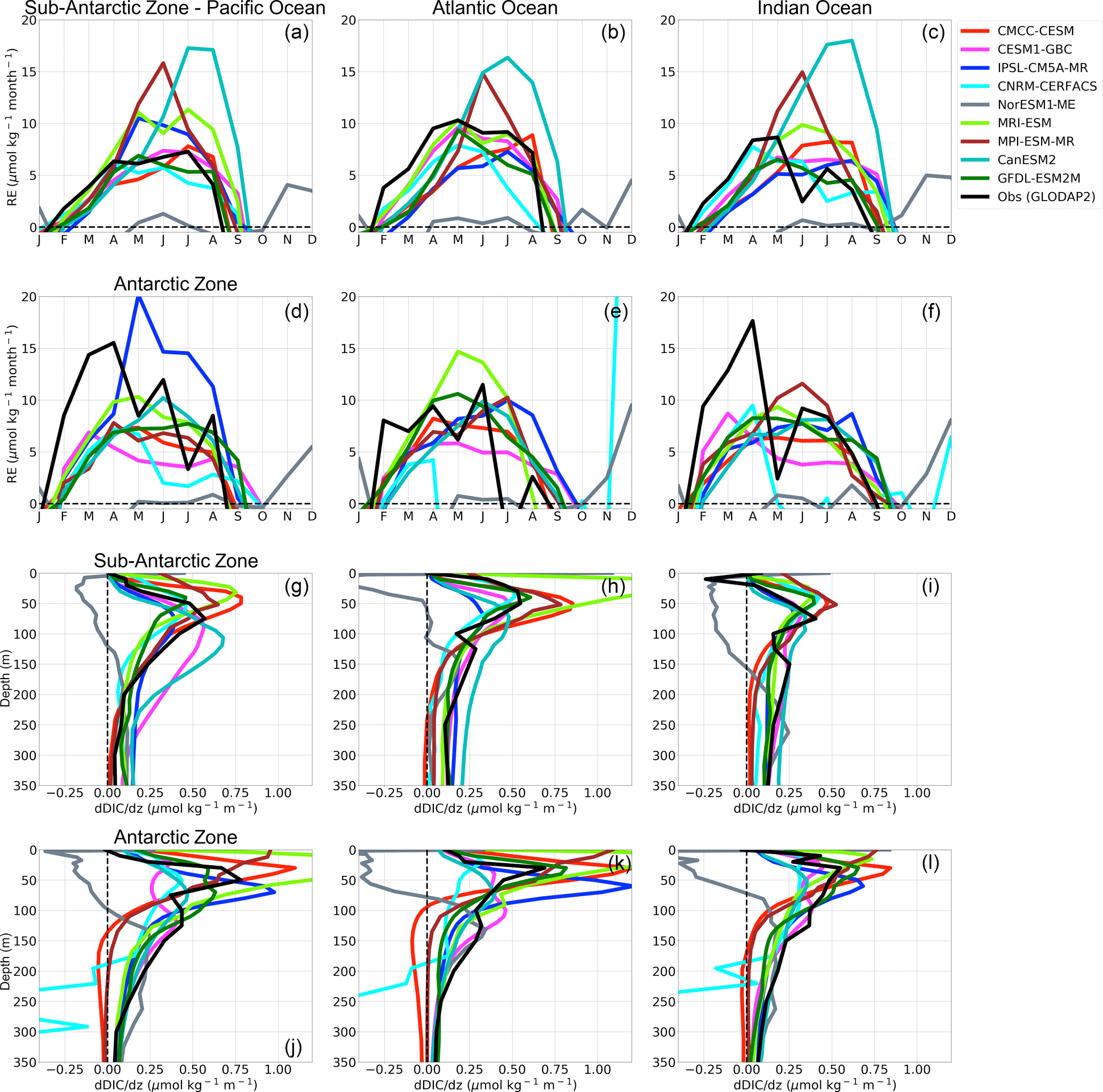
Figure 10 (a–f) Estimated DIC entrainment fluxes (mol kg month⁻¹) at the base of the mixed layer and (g–i) vertical DIC gradients (µmol kg⁻¹ m⁻¹) in the Sub-Antarctic and Antarctic zones of the Pacific Ocean (first column), Atlantic Ocean (second column) and Indian Ocean (third column).

In general terms, CMIP5 models are mostly in agreement (with an exception of MRI-ESM) with the observational product on the dominant role of DIC to regulating the seasonal cycle of FCO₂ (Fig. 6d–f), though not all models agree in the phase of the seasonal cycle of FCO₂ (e.g., CanESM2, Fig. 2). Though CMIP5 models still mostly show the SST rates biases in autumn and spring with respect to observed estimates, the stronger and near-surface vertical DIC maxima (Fig. 10) likely favor DIC as a dominant driver of FCO₂ changes. Differences between group-SST and group-DIC models are only evident in mid-summer, when SST rates heighten and primary production peaks (Fig. 3, 9). Probably because of sea ice presence, the onset of SST warming is a month later (November) here in comparison to the Sub-Antarctic (October). This subsequently allows the onset of primary production before the surface warming, which then permits the biological CO₂ uptake to be notable in group-SST models. Thus the two model groups here agree in the FCO₂ in-gassing during spring with group-SST models being the closest to the observational product. The MRI-ESM is the only model showing anomalous solubility dominance during autumn and spring as in the Sub-Antarctic Zone.

This coherence of CMIP5 models and observations in the Antarctic Zone may suggest that CMIP5 models compare better to observations in this region (Fig. 4). However, because CMIP5 models also show this spatial homogeneity in the Sub-Antarctic Zone (contrary to observational estimates), it is not clear whether this indicates an improved skill in CMIP5 model to the mechanisms of FCO₂ in this region, or whether both CMIP5 models and the observational product lack spatial sensitivity to the drivers of FCO₂. The sparseness of observations in the AZ points to the latter.

The cause of differences in the seasonal rates of SST change in group-SST models remains a subject of ongoing research. The Southern Ocean is a part of the global ocean (upwelling), where Earth systems models show a persistent warming SST bias (Hirahara et al., 2014). Several studies highlight potential explanations, but the main reasons remain uncertain. For example, CMIP5 model differences in the magnitude and meridional location of the peak of wind speeds in the Southern Ocean (Bracegirdle et al., 2013) and MLD differences (Meijers, 2014; Sallée et al., 2013) may be such that the net effect of change on surface turbulence and mixing leads to these amplified surface temperature rates. Other known CMIP5 models' biases that may contribute includes heat fluxes and storage (Frölicher et al., 2015) as well as sea-ice dynamics (Turner et al., 2013). Notwithstanding these, investigation of the reasons for sources of these dSST ∕ dt biases is out of the scope of this study. Our aim here is to show that understanding biases in the drivers of pCO₂ (DIC and SST) at the seasonal scale is necessary to understand differences in the seasonal cycle of FCO₂ between models and observational products. However, we recommend that the mechanistic basis for the differences in the seasonal rates of warming and cooling be urgently investigated further

5 Synthesis

We used a seasonal cycle framework to highlight and examine two major biases in respect of pCO₂ and FCO₂ in 10 CMIP5 models in the Southern Ocean.

Firstly, we examined the general exaggeration of the seasonal rates of change of SST in autumn and spring seasons during peak cooling and warming, respectively, with respect to available observations. These elevated rates of SST change tip the control of the seasonal cycle of pCO₂ and FCO₂ towards SST from DIC and result in a divergence between the observed and modeled seasonal cycles, particularly in the Sub-Antarctic Zone. While almost all analyzed models (9 of 10) show these SST-driven biases, 3 of the 10 (namely NorESM1-ME, HadGEM-ES and MPI-ESM) do not show these solubility biases because of their overly exaggerated primary production (and remineralization) rates such that biologically driven DIC changes mainly regulate the seasonal cycle of FCO₂. These models reproduce the observed phasing of FCO₂ as a result of an incorrect scaling of the biogeochemical fluxes. In the Antarctic Zone, CMIP5 models compare better with observations relative to the Sub-Antarctic Zone. This is mostly because both CMIP5 models and observational product estimates show a spatial and temporal uniformity in the characteristics of FCO₂ in the Antarctic Zone. However, it is not certain if this is because model process dynamics perform better in this high-latitude zone or that the observational products variability is itself limited by the lack of in situ data. This remains an open question that needs to be explored further and highlights the need for increased scale-sensitive and independent observations south of the PF and into the sea-ice zone.

The second major bias is that contrary to observational products estimates, CMIP5 models generally show an equal sensitivity to basin-scale FCO₂ drivers (except for CMCC-ESM, GFDL-ESM2M and CESM1-BGC) and hence the seasonal cycle of FCO₂ has similar phasing in all three basins of the Sub-Antarctic Zone. This is in contrast to observational and remote sensing products that highlight strong seasonal and interannually varying basin contrasts in both pCO₂ and phytoplankton biomass. It is not clear if this is due to inadequate carbon process parameterization or improper representation of the dynamics of the physics. This should be investigated further with CMIP6 models, and our analysis framework is proposed as a useful tool to diagnose the dominant drivers. Contrary to observed estimates, CMIP5 models simulate FCO₂ seasonal dynamics that are zonally homogeneous, and we suggest that any investigation of local (basin-scale) mechanisms, dynamics and long-term trends of FCO₂ using CMIP5 models must remain tentative and should be treated with caution. This highlights a key area of development for the next generation of models such as those planned to be used for CMIP6.