Upside-down fluxes Down Under: CO₂ net sink in winter and net source in summer in a temperate evergreen broadleaf forest

Predicting the seasonal dynamics of ecosystem carbon fluxes is challenging in broadleaved evergreen forests because of their moderate climates and subtle changes in canopy phenology. We assessed the climatic and biotic drivers of the seasonality of net ecosystem–atmosphere CO₂ exchange (NEE) of a eucalyptus-dominated forest near Sydney, Australia, using the eddy covariance method. The climate is characterised by a mean annual precipitation of 800 mm and a mean annual temperature of 18 ^∘C, hot summers and mild winters, with highly variable precipitation. In the 4-year study, the ecosystem was a sink each year (−225 g C m⁻² yr⁻¹ on average, with a standard deviation of 108 g C m⁻² yr⁻¹); inter-annual variations were not related to meteorological conditions. Daily net C uptake was always detected during the cooler, drier winter months (June through August), while net C loss occurred during the warmer, wetter summer months (December through February). Gross primary productivity (GPP) seasonality was low, despite longer days with higher light intensity in summer, because vapour pressure deficit (D) and air temperature (T_a) restricted surface conductance during summer while winter temperatures were still high enough to support photosynthesis. Maximum GPP during ideal environmental conditions was significantly correlated with remotely sensed enhanced vegetation index (EVI; r² = 0.46) and with canopy leaf area index (LAI; r² = 0.29), which increased rapidly after mid-summer rainfall events. Ecosystem respiration (ER) was highest during summer in wet soils and lowest during winter months. ER had larger seasonal amplitude compared to GPP, and therefore drove the seasonal variation of NEE. Because summer carbon uptake may become increasingly limited by atmospheric demand and high temperature, and because ecosystem respiration could be enhanced by rising temperatures, our results suggest the potential for large-scale seasonal shifts in NEE in sclerophyll vegetation under climate change.

1 Introduction

Forests and semi-arid biomes are responsible for the majority of global carbon storage by terrestrial ecosystems (Dixon et al., 1994; Pan et al., 2011; Poulter et al., 2014; Schimel et al., 2001). Photosynthesis and respiration by these biomes strongly influence the seasonal cycle of atmospheric CO₂ (Baldocchi et al., 2016; Keeling et al., 2005). Continuous measurements of land–atmosphere exchanges of carbon, energy and water provide insights into the seasonality of forest ecosystem processes, which are driven by the interactions of climate, plant physiology and forest composition and structure (Xia et al., 2015). Net ecosystem exchange (NEE) seasonality is relatively well understood in cool-temperate ecosystems; deciduous trees can only photosynthesise when they have leaves and NEE dynamics are thus principally influenced by the phenology of canopy processes. NEE of deciduous forests thus has a more pronounced seasonality than that of evergreen conifer forests at similar latitudes (Novick et al., 2015). For high-latitude evergreen conifer forests, NEE seasonality is strongly limited by cold temperature limitation of photosynthesis (Kolari et al., 2007) and respiration. In contrast, seasonality of NEE in evergreen broadleaf forests, typically occurring in warm-temperate and tropical regions, is much less well understood (Restrepo-Coupe et al., 2017; Wu et al., 2016).

The seasonality of gross primary productivity (GPP) in evergreen broadleaf forests may be driven by climate (e.g. dry/wet seasons) and/or by canopy dynamics (Wu et al., 2016). In tropical evergreen forests, air temperature and day length are similar seasonally, but precipitation seasonality can be strong, with higher radiation and temperature (1 or 2 ^∘C higher) in the dry season (Trenberth, 1983; Windsor, 1990). Counter-intuitively, GPP can be higher during the dry season, as cloud cover may limit productivity in the wet season (Graham et al., 2003; Hutyra et al., 2007; Saleska et al., 2003). Canopy dynamics can be an important determinant of GPP seasonality in evergreen broadleaf forests; although leaves are present in the canopy year-round in evergreen canopies, leaf area index (LAI) may show considerable temporal variability seasonally as new leaves are produced and old leaves die, especially during leaf flush and senescence periods (Duursma et al., 2016; Wu et al., 2016). Both leaf light use efficiency and water use efficiency may vary as leaves age: young leaves and old leaves are less efficient than mature leaves, reflecting changes in photosynthetic capacity (Wilson et al., 2001; Wu et al., 2016). The timing of leaf flush and senescence can depend on the environment and on species; environmental stress, such as drought, can induce the process of senescence (Lim et al., 2007; Munné-Bosch and Alegre, 2004).

In temperate evergreen broadleaved forests, such as eucalypt-dominated sclerophyll vegetation in Australia, precipitation can be seasonal or aseasonal; furthermore, day length and temperature vary significantly between winter and summer. GPP can be limited by frost during winter and by drought during summer. Atmospheric demand indicated by high vapour pressure deficit (D) and soil drought have different impacts on GPP, but they can interact to impact surface conductance (G_s; Medlyn et al., 2011; Novick et al., 2016). In Australia's temperate eucalypt forests, canopy rejuvenation takes place in summer and is linked to heavy rainfall events (Duursma et al., 2016). However, since leaf flushing and shedding occur simultaneously in eucalypt canopies (Duursma et al., 2016; Pook, 1984), the overall canopy volume can remain stable while the distribution of canopy volume changes with height (Griebel et al., 2015). Eucalypt forests in southeast Australia have been found to act as carbon sinks all year long, with greater uptake in summer (Hinko-Najera et al., 2017; van Gorsel et al., 2013). Although canopy characteristics are key to understanding ecosystem fluxes, their dynamics in Australian ecosystems can be particularly challenging to detect using standard vegetation indices (Moore et al., 2016). Nevertheless, the normalised difference vegetation index (NDVI) has successfully explained variability in photosynthetic capacity in Mediterranean, mulga and savanna ecosystems (Restrepo-Coupe et al., 2016).

The environmental and biotic controls on the seasonal dynamics of ecosystem fluxes in broadleaved evergreen forests are still poorly understood. Our objective was to determine the seasonality of ecosystem CO₂ and H₂O fluxes in a dry sclerophyll Eucalyptus forest; we evaluated the role of environmental drivers (photosynthetic photon flux density, PPFD; T_a; soil water content, SWC; D) and canopy dynamics (as measured with EVI, LAI, litter fall and leaf age) in regulating the seasonal patterns of NEE, GPP, ecosystem respiration (ER), evapotranspiration (ET) and surface conductance (G_s) in an evergreen forest near Sydney, Australia. We also compared leaf-level to ecosystem-level water and carbon exchange in response to drivers, in order to gain confidence in our results and gain insights into the emergent properties from leaf to ecosystem scale. We hypothesised that canopy phenology (LAI and leaf age) explains temporal variation in photosynthetic capacity (PC) and G_s. We anticipated that the ecosystem would be a carbon sink all year long.

2 Materials and methods

2.1 Site description

The field site is the Cumberland Plain (AU-Cum in Fluxnet) forest SuperSite (Resco de Dios et al., 2015) of the Australian Terrestrial Ecosystem Research Network (http://www.ozflux.org.au, last access: 12 June 2018), located 50 km west of Sydney, Australia, at 23 m elevation, on a nearly flat floodplain of the Nepean–Hawkesbury River (latitude −33.61518; longitude 150.72362). Mean mid-afternoon (15:00 local standard time) temperature is 18 ^∘C (max. 28.5 ^∘C in January and min. 16.5 ^∘C in July) and average precipitation is 801 mm yr⁻¹ (mean monthly max. is 96 mm in January, and min. is 42 mm in September). The soil is classified as a Kandosol and consists of a fine sandy loam A horizon (0–8 cm) over clay to clay loam subsoil (8–40 cm), with pH of 5 to 6 and up to 5 % organic C in the top 10 cm (Karan et al., 2016). The flux tower is in a mature dry sclerophyll forest, with 140 Mg C ha⁻¹ aboveground biomass and a stand density of ∼ 500 trees ha⁻¹. The stand hosts a large population of mistletoe (Amyema miquelii), which decreases in abundance with increasing distance from the flux tower. The canopy structure comprises three strata, and the predominant canopy tree species are Eucalyptus moluccana and E. fibrosa. While individual trees can exceed 25 m height, an airborne lidar survey from November 2015 indicates an average canopy height of ∼ 24 m within a 300 m radius of the flux tower (Fig. S1 in the Supplement). The mid-canopy stratum (5–12 m) is dominated by Melaleuca decora and the understory is dominated by Bursaria spinosa with various shrubs, forbs, grasses and ferns present in lower abundance.

2.2 Environmental measurements

Air temperature (T_a) and relative humidity (RH) were measured using HMP45C and HMP155A (Vaisala, Vantaa, Finland) sensors at 7 and 29 m heights respectively. Vapour pressure deficit (D) was estimated from T_a and RH. The PPFD above the canopy (µmol m⁻² s⁻¹) was measured using an LI190SB (Licor Inc., Lincoln, NE, USA), and incoming and outgoing shortwave and longwave radiation were measured using a CNR4 radiometer (Kipp & Zonen, Delft, the Netherlands). Ancillary data were logged on CR1000 or CR3000 data loggers (Campbell Scientific, Logan, UT, USA) at 30 min intervals. Mixing ratios of CO₂ in air were also measured at 0.5, 1, 2, 3.5, 7, 12, 20 and 29 m above the soil surface using a LI840A Gas Analyzer (Licor Inc., Lincoln, NE, USA); data from each height were logged on a CR1000 data logger once every 30 min (1 min air sampling per height).

Ground heat flux and soil moisture were averaged between two locations to represent the variable shading in the tower footprint. One location had a HFP01 heat flux plate and the other had a self-calibrating heat flux plate (HFP01SC; Hukseflux, XJ Delft, the Netherlands) installed at 8 cm below the soil surface. The heat flux plates were paired with a CS616 water content reflectometer (Campbell Scientific, Logan UT) installed horizontally at 5 cm below the soil surface and an averaging thermocouple (model TCAV, Campbell Scientific, Logan, UT, USA) installed with thermocouples at 2 and 6 cm below the soil surface for each pair. Another CS616 was installed vertically to measure average soil water content from 7 to 37 cm (CS616). Rainfall was measured at an open area with a tipping bucket 2 km away from the study site.

2.3 Net ecosystem exchange

Continuous land–atmosphere exchange of CO₂ mass (NEE) was quantified from direct measurements of the different components of the theoretical mass balance of CO₂ in a control volume:

$$\begin{array}{}\text{(1)}& \mathrm{NEE}=F_{\mathrm{CT}}+F_{\mathrm{CS}},\end{array}$$

where F_CT is the vertical turbulent exchange flux, and F_CS is the change in storage flux. Advection fluxes are assumed negligible when atmospheric turbulence is sufficient (Aubinet et al., 2012; Baldocchi et al., 1988), and when quality control (QC) flags of stationarity and turbulence development test were good (Foken et al., 2004). We used change-point detection of the friction velocity (u^∗) threshold (Barr et al., 2013) to determine the turbulence threshold above which NEE (the sum of F_CT and F_CS) is independent of u^∗. However, we found no clear dependence of NEE on u^∗ and hence no clear threshold (Fig. S2), so we used a threshold of 0.2 m s⁻¹ to be conservative.

The calculation of each term, and the assumptions required for them to be representative of each half-hour flux are detailed below.

2.4 Vertical turbulent flux (F_CT)

The vertical turbulent fluxes of CO₂ (F_CT, µmol m⁻² s⁻¹) and water (F_WT, mmol m⁻² s⁻¹) were measured using the eddy covariance method (Baldocchi et al., 1988). Density (c) of CO₂ or water vapour (open-path IRGA, LI-7500A, Licor Inc., Lincoln, NE, USA) and vertical wind speed (w; CSAT 3D sonic anemometer, Campbell Scientific, Logan, UT, USA) were measured at 10 Hz frequency at 29 m above the ground, and logged on a CR-3000 data logger (Campbell Scientific, Logan, UT, USA). Vertical turbulent fluxes were calculated from the 10 Hz data, using EddyPro© software. Statistical tests for raw data screening included spike count/removal, amplitude resolution, drop-outs, absolute limits and skewness and kurtosis tests (Vickers and Mahrt, 1997). Low- and high-frequency spectral correction followed Moncrieff et al. (2004, 1997). The calculation allowed for up to 10 % of missing 10 Hz data. Fluxes were rotated into the natural wind coordinate system using the double rotation method (Wilczak et al., 2001). We compensated for time lags between the sonic and IRGA by using covariance maximisation, within a window of plausible time lags (Fan et al., 1990). We applied the block averaging method to calculate each half-hour average and fluctuation relative to the average, to calculate the covariance (Gash and Culf, 1996). Density fluctuations in the air volume were corrected using the WPL terms (Webb et al., 1980). Each half-hourly flux was associated with a QC flag (0: good quality; 1: keep for integrations, discard for empirical relationships; 2: remove from the data); these flags accounted for stationarity tests and turbulence development tests which are required for good turbulent flux measurements (Foken et al., 2004). In our 4-year record, 51 % of F_CT fluxes had a flag of 0, 32 % had a flag of 1 and 17 % had a flag of 2. Although the tower height (29 m) is rather close to the average canopy height (24 m), cospectra analysis showed good quality turbulent fluxes (the high frequency followed the $-\mathrm{4}/\mathrm{3}$ slope; thus we did not find any indications of systematic dampening in the cospectra; see Fig. S3).

2.5 Storage flux (F_CS)

The change in storage flux (F_CS, µmol m⁻² s⁻¹) was measured using a CO₂ profiler system, such that change of storage flux timestamp was the same as the turbulent flux timestamp.

The change in storage flux was calculated as (Aubinet et al., 2001):

$$\begin{array}{}\text{(2)}& F_{\mathrm{CS}}={\displaystyle \frac{P_{\mathrm{a}}}{R{T}_{\mathrm{a}}}}\underset{\mathrm{0}}{\overset{h}{\int }}{\displaystyle \frac{\mathrm{d}C\left(z\right)}{\mathrm{d}t}}\mathrm{d}z,\end{array}$$

where P_a is the atmospheric pressure (P_a), T_a is the temperature (K), R is the molar gas constant and C(z) is CO₂ (µmol m⁻³) at the height z. CO₂ is measured in ppm and converted to µmol m⁻³ using ideal gas law equation, where the air temperature and air pressure at each inlet are estimated from a linear interpolation between sensors at the top of the tower (29 m) and sensors at the bottom of the tower (7 m). As we only measure a limited number of heights, in practice this equation becomes

$$\begin{array}{ll}{\displaystyle }& {\displaystyle }{F}_{\mathrm{CS}}={\left({\displaystyle \frac{\mathrm{\Delta }C}{\mathrm{\Delta }t}}\right)}_{k=\mathrm{1}}\times z_{k=\mathrm{1}}\\ \text{(3)}& {\displaystyle }& {\displaystyle }+{\sum }_{k=\mathrm{2}}^n\left\{\left[{\left({\displaystyle \frac{\mathrm{\Delta }C}{\mathrm{\Delta }t}}\right)}_k+{\left({\displaystyle \frac{\mathrm{\Delta }C}{\mathrm{\Delta }t}}\right)}_{k-\mathrm{1}}\right]\times {\displaystyle \frac{z_k-z_{k-\mathrm{1}}}{\mathrm{2}}}\right\},\end{array}$$

where C is CO₂ (µmol m⁻³) and t is time (s; ΔC∕Δt is the variation of C over 30 min), z is the height (m) and k [1 to n = 8] represents each inlet. We flagged and replaced the storage flux with a one-point approximation during profiler outages (25 % of the 4-year record), using the change in CO₂ at 29 m height over 30 min as derived in EddyPro (Aubinet et al., 2001). These data were not used for empirical relationships, but kept for annual sum calculations. Storage flux of water vapour was assumed to be negligible. For visualisation of the diurnal course of storage flux and turbulent flux, see Fig. S4.

2.6 Gap-filling of environmental variables and NEE separation into gross fluxes

We used the PyFluxPro software for gap-filling climatic variables and fluxes, and for partitioning the NEE into GPP and ER (Isaac et al., 2017). We only used observational data that passed the steady state and developed turbulence tests for gap-filling and for partitioning (QC flags of 0 and 1; Foken et al., 2004). In brief, gaps in climate variables were filled following the hierarchy of using variables provided from (1) automatic weather stations from the closest weather station, (2) numerical weather prediction model outputs (ACCESS regional, 12.5 km grid size provided by the Bureau of Meteorology) and lastly (3) monthly mean values from the site-specific climatology. In the next step the continuous climate variables were used to fill all fluxes by utilising the embedded SOLO neural network with 25 nodes and 500 iterations on monthly windows. We used the random forest method (Breiman, 2001) to determine and rank potential explanatory variables for explaining latent heat flux (λE), sensible heat flux (H) and NEE. We then selected the five variables with the highest feature importance for each flux and compared the gap-filling performance of the neural network for each flux with the performance based on an educated guess of potential relevant drivers. We selected the variable array with the highest Pearson correlation coefficient (r) and lowest root mean square error (RMSE) for gap-filling in PyFluxPro, which identified net radiation (R_n), SWC, soil temperature (T_s), wind speed (w_s) and vapour pressure deficit (D) for λE (r = 0.93, RMSE = 32.0); down-welling shortwave radiation (F_sd), air temperature (T_a), T_s, w_s , SWC and D for H (r = 0.97, RMSE = 23.1); F_sd, D, T_a, T_s and SWC for NEE (r = 0.87, RMSE = 4.04). To gap-fill ER, all nocturnal observational data (at night, we assume GPP = 0 so NEE = ER) that passed all QC checks and the u^∗ filter were modelled using T_s, T_a and SWC as drivers in SOLO on the full dataset with 10 nodes and 500 iterations. Lastly, this gap-filled ER was used to infer GPP as the result of NEE − ER.

2.7 Flux footprint

We analysed the footprint climatology of Cumberland Plain site according to Kormann and Meixner (2001), using the R-Package “FREddyPro” (Fig. S5). We assumed that the ecosystem within the footprint was homogeneous for the purpose of this study and found that, after u^∗ filtering, CO₂ turbulent fluxes (F_CT) originated from the footprint of interest.

2.8 Energy balance

We evaluated the energy balance closure with the ratio of available energy (R_n − soil heat flux, G) to the sum of turbulent heat fluxes (λE+H). On a daily basis, the energy balance closure was 70 % (Fig. S6), consistent with the well-known and common issue of a lack of closure (Foken, 2008; Foken et al., 2006; Wilson et al., 2002). We did not use the criteria that closure had to be met for the reported fluxes.

2.9 Surface conductance

Surface conductance (G_s) was derived by inverting the Penman–Monteith equation (Monteith, 1965):

$$\begin{array}{}\text{(4)}& G_{\mathrm{s}}={\displaystyle \frac{\mathit{\gamma }\mathit{\lambda }E{g}_{\mathrm{a}}}{\mathrm{\Delta }{R}_{\mathrm{n}}+\mathit{\rho }{C}_{p}D{g}_{\mathrm{a}}-\mathit{\lambda }E\left(\mathrm{\Delta }+\mathit{\gamma }\right)}},\end{array}$$

where γ is the temperature-dependent psychrometric constant (kPa K⁻¹), λE is the latent heat flux (W m⁻²), Δ is the temperature-dependent slope of the saturation–vapour pressure curve (kPa K⁻¹), R_n is net radiation (W m⁻²), ρ is the dry air density (kg m⁻³), D is vapour pressure deficit (kPa), C_p is the specific heat of air (J kg⁻¹ K⁻¹) and g_a is the bulk aerodynamic conductance, formulated as an empirical relation of mean horizontal wind speed (U, m s⁻¹) and friction velocity (u^∗, m s⁻¹; Thom, 1972):

$$\begin{array}{}\text{(5)}& g_{\mathrm{a}}={\displaystyle \frac{\mathrm{1}}{\frac{U}{u^{{\ast }^{\mathrm{2}}}}+\mathrm{6.2}{u}^{{\ast }^{-\mathrm{0.67}}}}}.\end{array}$$

In the analysis for G_s, we were interested in transpiration (T) rather than evaporation (E), so we excluded data if precipitation exceeded 1 mm in the past 2 days, 0.5 mm in the past 24 h and 0.2 mm in the past 12 h (Knauer et al., 2015). We assumed that evaporation (E) was negligible using these criteria (Knauer et al., 2018), which excluded 40 % of the data.

2.10 Dynamics of canopy phenology (leaf area index, and litter and leaf production) and photosynthetic capacity

We evaluated the dynamics of canopy LAI by measuring canopy light transmittance with three under-canopy PPFD sensors and one above-canopy PPFD sensor LI190SB (Licor Inc., Lincoln, NE, USA) following the methods presented in Duursma et al. (2016). Although we use the term LAI, this estimate does include non-leaf surface area (stems, branches). We collected litterfall (L_f, g m² month⁻¹) in the tower footprint approximately once per month, from nine litter traps (0.14 m⁻² ground area) located near the understory PPFD sensors. We estimated specific leaf area (SLA) of eucalyptus and mistletoe leaves by sampling approximately 50 fresh leaves of each, in June 2017 (SLA = 56.4 cm² g⁻¹ for eucalyptus, 40.3 cm² g⁻¹ for mistletoe). For each month, we partitioned the litter into eucalyptus leaves, mistletoe leaves and other (mostly woody) components. We used this SLA to estimate leaf litter production (L_p) in m² m⁻² month⁻¹ of eucalyptus, mistletoe and total as the sum of both. Then, we estimated leaf growth (L_g, m² month⁻²) as the sum of the net change in LAI (ΔL) and L_p. Photosynthetic capacity (PC) is defined as median GPP when PPFD is 800–1200 µmol m⁻² s⁻¹ and D is 1.0 to 1.5 kPa.

2.11 Analysis of light response of NEE

We evaluated the light response of NEE using a saturating exponential function (Eq. 5) to test whether parameters varied between seasons (Aubinet et al., 2001; Lindroth et al., 2008; Mitscherlich, 1909).

$$\begin{array}{ll}{\displaystyle }\mathrm{NEE}=& {\displaystyle }-\left({\mathrm{NEE}}_{\mathrm{sat}}+R_d\right)\left(\mathrm{1}-\exp \left[{\displaystyle \frac{-\mathit{\alpha }\mathrm{PPFD}}{{\mathrm{NEE}}_{\mathrm{sat}}+R_d}}\right]\right)\\ \text{(6)}& {\displaystyle }& {\displaystyle }+R_d,\end{array}$$

where the parameter R_d is the intercept, or NEE in the absence of light, often called dark respiration; NEE_sat is NEE at light saturation and α is the initial slope of the curve, expressed in µmol CO₂ µmol photon⁻¹ and representing light use efficiency when photosynthetic photon flux density (PPFD) is close to 0. We only used daytime quality-checked NEE data to fit the model (QC = 0; Foken et al., 2004, LI-7500 signal strength = max, all inlets of profiler system data available and u^∗ > 0.2 m s⁻¹); see Fig. S7.

2.12 Leaf gas exchange spot measurements

We used previously published data of spot leaf gas exchange measurements in a nearby site for comparison with ecosystem fluxes (Gimeno et al., 2016).

Figure 1 (a) Time series of monthly carbon flux (NEE, ER and GPP, g C m⁻² month⁻¹; negative indicates ecosystem uptake); (b) rainfall, mm month⁻¹; soil water content from 0 to 8 cm (SWC_0–8 cm, %); (c) average of daily maximum for each month photosynthetically active radiation (PPFD_max, µmol m⁻² s⁻¹), air temperature (T_a,max, ^∘C) and vapour pressure deficit (D_max, kPa). (d) Canopy dynamics trends: enhanced vegetation index (EVI, unitless); LAI (m² m⁻²) and litter production (L_p, m² m⁻² month⁻¹). Shaded areas shows summer (dark grey) and winter (light grey). Note T_a,max and PPFD_max remained above 15 ^∘C and 800 µmol m⁻² s⁻¹.

2.13 Remotely sensed land surface greenness

Normalised difference vegetation index (NDVI) and Enhanced Vegetation Index (EVI) values were derived from the MODIS Terra Vegetation Indices 16-Day L3 Global 250 m product (MOD13Q1), which uses atmospherically corrected surface reflectance masked for water, clouds, heavy aerosols, and cloud shadows (Didan, 2015). At 250 m spatial resolution, the pixel containing Cumberland Plain was assumed to be representative for the footprint and values of that pixel between 1 January 2014 and 31 December 2017 were extracted.

3 Results

3.1 Seasonality of environmental drivers and leaf area index

Climatic conditions were favourable for growth at the site year-round. The monthly average of daily maximum air temperature was 16.3 ^∘C during the coldest month (July, 2015), and the lowest monthly average of daily maximum PPFD was 878 µmol m⁻² s⁻¹ in the winter (June 2015; Fig. 1c). Although less rainfall occurred during winter months compared to summer months, precipitation occurred throughout the year (Fig. 1b). Soil volumetric water content (SWC) in the shallow (0–8 cm) layer was about 10 % except immediately following rain events (Fig. 1b). In contrast, SWC in the clay layer (8–38 cm) remained above 30 % for the duration of the study (data not shown). Monthly average of daily maximum air temperature ranged from 16.3 ^∘C in July 2015 to 32.7 ^∘C in January 2017; monthly average of daily maximum D ranged from 0.9 kPa in June 2015 to 3.4 kPa in January 2017 (Fig. 1c). For visualisation of seasonal and diurnal trends of radiation, air temperature, D and SWC, see Fig. S8.

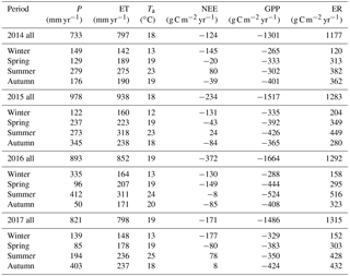
Table 1 Annual precipitation (P, mm yr⁻¹), ET (mm yr⁻¹), air temperature T_a (^∘C), NEE (g C m⁻² yr⁻¹), GPP (g C m⁻² yr⁻¹) and ER (g C m⁻² yr⁻¹) for the 4-year study period.

Canopy LAI varied between 0.7 (in December 2014) and 1.15 m² m⁻² (in March 2016 and June 2017; Fig. 1d). LAI followed a distinct pattern: it peaked in late summer (around February), and then continuously decreased until the new leaves emerged the following year. A late leaf flush was observed in 2017 (May). Litter production also peaked in summer, before and during the leaf flush, and was lower in winter (Fig. 1d). EVI followed the time dynamic of LAI.

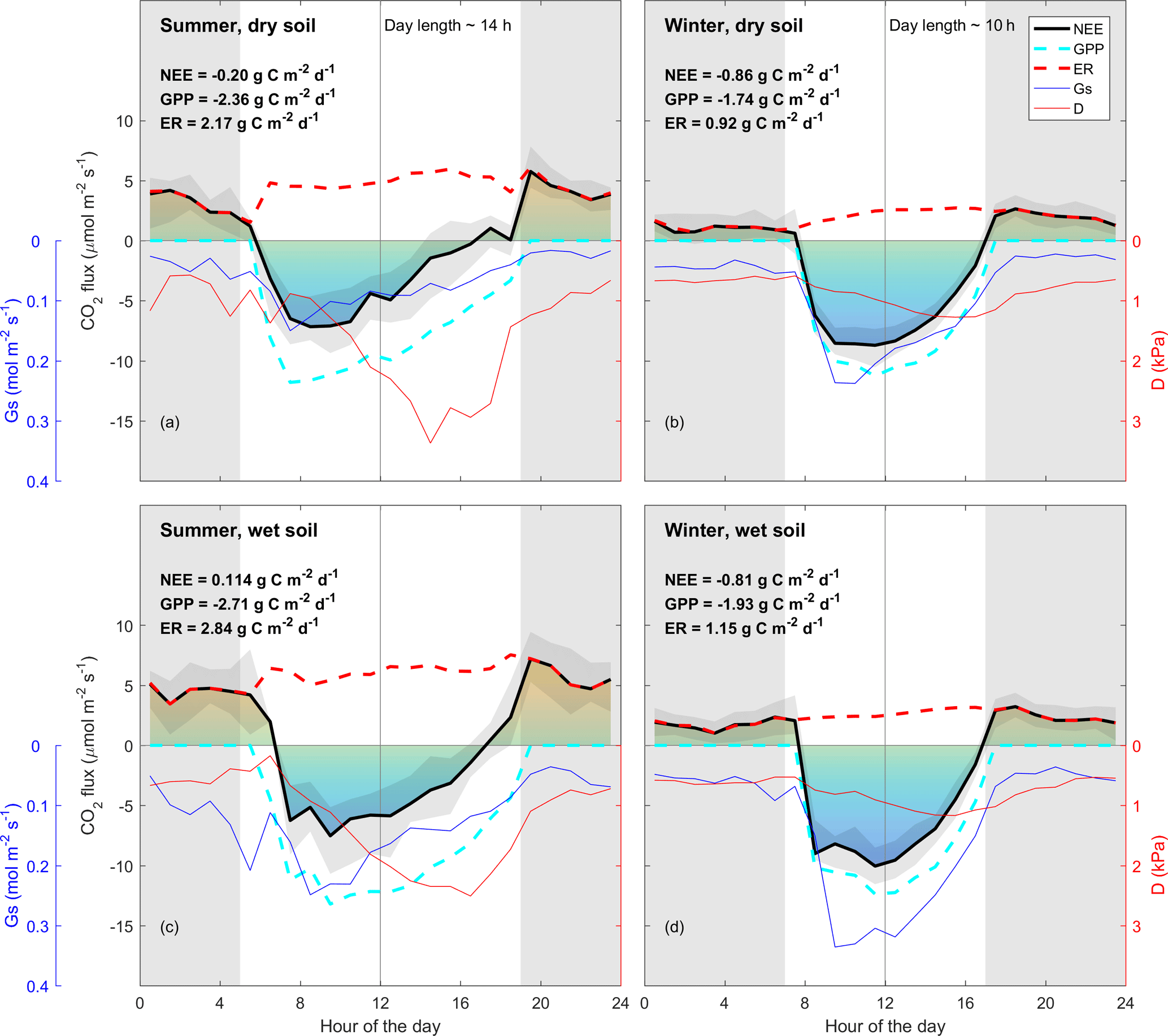
Figure 2 Diurnal trend (line: median; shade: quartile) of clear-sky-measured NEE (thick black line, µmol m⁻² s⁻¹); estimated daytime ecosystem respiration (ER, inferred from a neural network fitted on nighttime NEE, thick dotted red line, µmol m⁻² s⁻¹); estimated GPP (inferred as NEE − estimated daytime ER, thick dotted cyan line, µmol m⁻² s⁻¹); measured vapour pressure deficit (D, thin red line, kPa); estimated surface conductance (G_s, inferred from Penman–Monteith, blue line, mmol m⁻² s⁻¹). Grey shade shows night-time (sunset to sunrise). NEE, GPP and ER number are calculated by integrating the diurnal fluxes as shown in the figure. “Wet” and “dry” soil is defined as below or above the median of soil water content during summer or winter. Summer is December through February. Winter is June through August, as defined by the Sydney Bureau Of Meteorology. Colours under NEE rate are shown for visualisation. Note that there is asymmetry between morning and afternoon NEE in summer, and less so in winter. Note that ecosystem respiration (nighttime NEE) is enhanced by SWC in summer, and less so in winter. Data used in this figure correspond to clear-sky half-hour values, where high-quality data measured for NEE were available.

3.2 Seasonality of carbon and water fluxes

Contrary to expectations, the ecosystem was always a sink for carbon in winter (−146 g C m⁻² on average, with a standard deviation of 22 g C m⁻²), and usually a carbon source or close to neutral in summer (+44 g C m⁻² on average, with a standard deviation of 43 g C m⁻²; Table 1). On average, summer GPP was lower, i.e. more uptake (−400 ± 97 g C m⁻²) compared to winter GPP (−282 ± 41 g C m⁻²; Table 1), a difference of ∼ 118 g C m⁻². However, average summer ER was much higher (444 ± 56 g C m⁻²) compared to winter ER (159 ± 35 g C m⁻²; Table 1), a difference of ∼ 285 g C m⁻². The summer vs. winter ER difference was more than double the GPP difference; thus, ER had a relatively larger effect over the seasonality of NEE.

3.3 Diurnal trend of CO₂ flux and drivers in winter and summer

The diurnal pattern of NEE in clear-sky conditions differed between summer and winter (Fig. 2). Relatively speaking, diurnal NEE was more symmetric in the winter than in summer. That is, morning and afternoon NEE patterns were mirror images and total integrated morning NEE was similar to integrated afternoon NEE during the winter, but strong hysteresis occurred in the summer (Fig. 2). This pattern also translated into hysteresis in the NEE light response curve in summer, but to a lesser degree in winter (Fig. 3).

3.4 Analysis of NEE light response curve

The parameters of the NEE light response in summer and winter are shown in Fig. 4 (see Sect. 2, Eq. 5). The initial slope of NEE with light (α) showed no clear dependence on T_soil in winter but exhibited sensitivity during summer, dropping precipitously at soil temperature above 23 ^∘C (Fig. 4a). α increased with SWC in winter and summer by a factor of 1.5 (Fig. 4b). In both winter and summer α decreased with D (D > 1 kPa) and in a similar fashion, approaching a saturating value of 0.01 (µmol µmol⁻¹) at a D of about 2 kPa (Fig. 4c). The fitted NEE at saturating light (NEE_sat) was not related to T_soil in winter but decreased with increasing T_soil in summer (Fig. 4d). NEE_sat was higher in winter than in summer for a given SWC. The relationship with D was more complicated, tending to increase with D in winter, but decreasing with increased D in summer, dropping from 9 to 3 µmol m⁻² s⁻¹ as D increased from 1 to 4 kPa. R_d was significantly higher in summer than winter across all conditions of T_soil, SWC and D (Fig. 4g, h, i). R_d increased with T_soil in winter and less so in summer. In winter, R_d increased up to SWC of 11 %; in summer, R_d was more sensitive to SWC, doubling from a rate of ∼ 4 to ∼ 8 µmol m⁻² s⁻¹ as SWC increased from about 8 to 20 %.

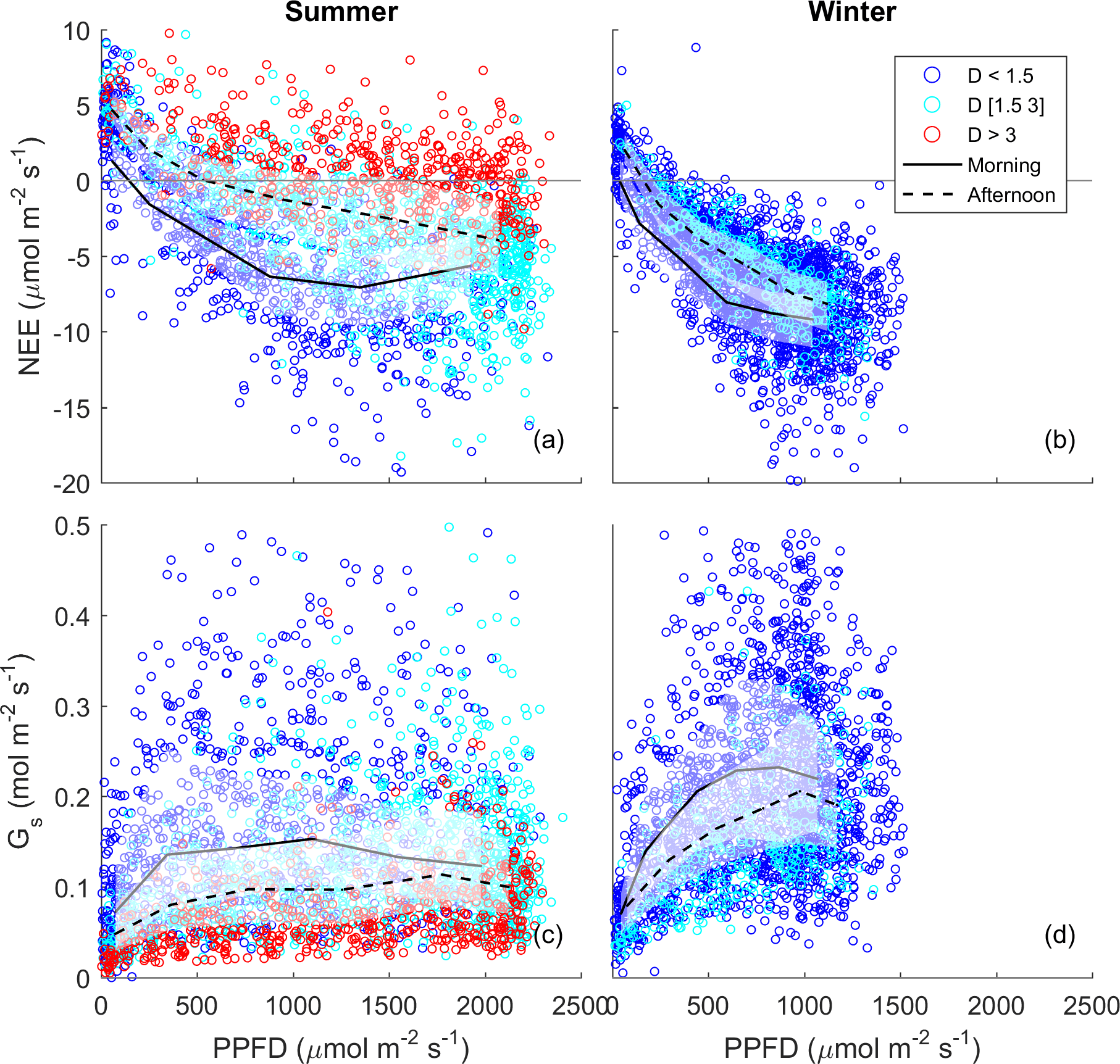
Figure 3 Half-hourly measured NEE vs. PPFD, coloured by D (blue: D < 1.5 kPa; cyan: D of 1.5–3 kPa; red: D > 3 kPa) for (a) summer and (b) winter periods. Raw data are binned by light levels to show median (lines) and quartiles (white shades) for morning (continuous lines) and afternoon (dotted lines) hours separately.

3.5 Atmospheric demand and soil drought control on GPP, ET, G_s and WUE

We evaluated the effect of SWC and vapour pressure deficit (D) on GPP, ET, water use efficiency (WUE) and surface conductance (G_s) under high radiation (“light-saturated”; PPFD > 1000 µmol m⁻² s⁻¹), after filtering periods following rain events in order to minimise the contribution of evaporation to ET (see Sect. 2; Fig. 5). In summer, light-saturated GPP decreased above D ∼ 1.3 kPa, but in winter, GPP did not vary with D. In summer and in winter, GPP increased with SWC (Fig. 5a). This is consistent with Fig. 4, where R_d and NEE_sat both increased with SWC. In summer, light-saturated ET increased with D up to ∼ 1.3 kPa, above which it reached a plateau. In winter, ET kept increasing with D, as D rarely exceeded 2 kPa. In both seasons, ET increased with SWC (Fig. 5b). Surface conductance decreased with D and SWC especially in summer, indicating strong stomatal regulation (Fig. 5d). WUE decreased with increasing D in summer and in winter, because ET increased but −GPP decreased (Fig. 5c).

Figure 4 NEE µmol m⁻² s⁻¹ light response parameters, calculated for different bins of climatic drivers (soil temperature (T_soil, ^∘C) at 5 cm depth, soil water content (SWC, %) from 0 to 8 cm depth and atmospheric demand (D, kPa) at 29 m height); only raw, QC-filtered daytime data are used. Light response curve was fitted using Mitscherlich equation (see Sect. 2); α is the initial slope, near PPFD = 0 (µmol µmol⁻¹); NEE_sat µmol m⁻² s⁻¹ is NEE at light saturation; R_d µmol m⁻² s⁻¹ is the dark respiration (NEE when PPFD = 0). Blue indicates winter months, and red indicates summer months. Dots are parameter values for each quartile of driver, plotted at x = median of driver for each bin. Shading is 95 % confidence interval of the parameter fit.

We compared these ecosystem-scale results to the equivalent at the leaf scale, which are net photosynthesis at light saturation A_max (PPFD ∼ 1800 µmol m⁻² s⁻¹), leaf transpiration T, leaf water use efficiency and stomatal conductance g_s (Fig. 5, black lines). These leaf level measurements are expressed on a leaf-area basis, as compared to ground area for ecosystem scale. We observed that A_max, T and g_s were more sensitive to D than corresponding ecosystem-scale responses. A_max was much higher than GPP_max at D ∼ 1 kPa, while g_s was comparable in magnitude to G_s in the same condition. Leaf transpiration peaked around D = 1.2 kPa, while ET plateaued. Leaf water use efficiency was overall higher than ecosystem WUE.

Figure 5 Gross primary productivity or net assimilation (GPP or Amax, µmol m⁻² (ground or leaf) s⁻¹), evapotranspiration or leaf transpiration (ET or T, mmol m⁻² (ground or leaf) s⁻¹), water use efficiency (WUE = GPP ∕ ET or $A_{max}/T$, µmol mmol⁻¹) and surface conductance or leaf conductance (G_s or g_s, mmol m⁻² s⁻¹) vs. vapour pressure deficit (D). Leaf level is shown in black; ecosystem scale is shown in colour (summer in red and winter in blue), at saturated PPFD (> 1000 µmol m⁻² s⁻¹). D is binned into four quartiles for ecosystem and eight for leaf; Y is mean value for each D bin, plotted at the median of D bin. Shaded area indicates the standard error of the mean. The three colour intensity show SWC quantiles (SWC < 0.33, SWC (0.33–0.67) and SWC (0.67–1.00) shown in decreasing colour intensity).

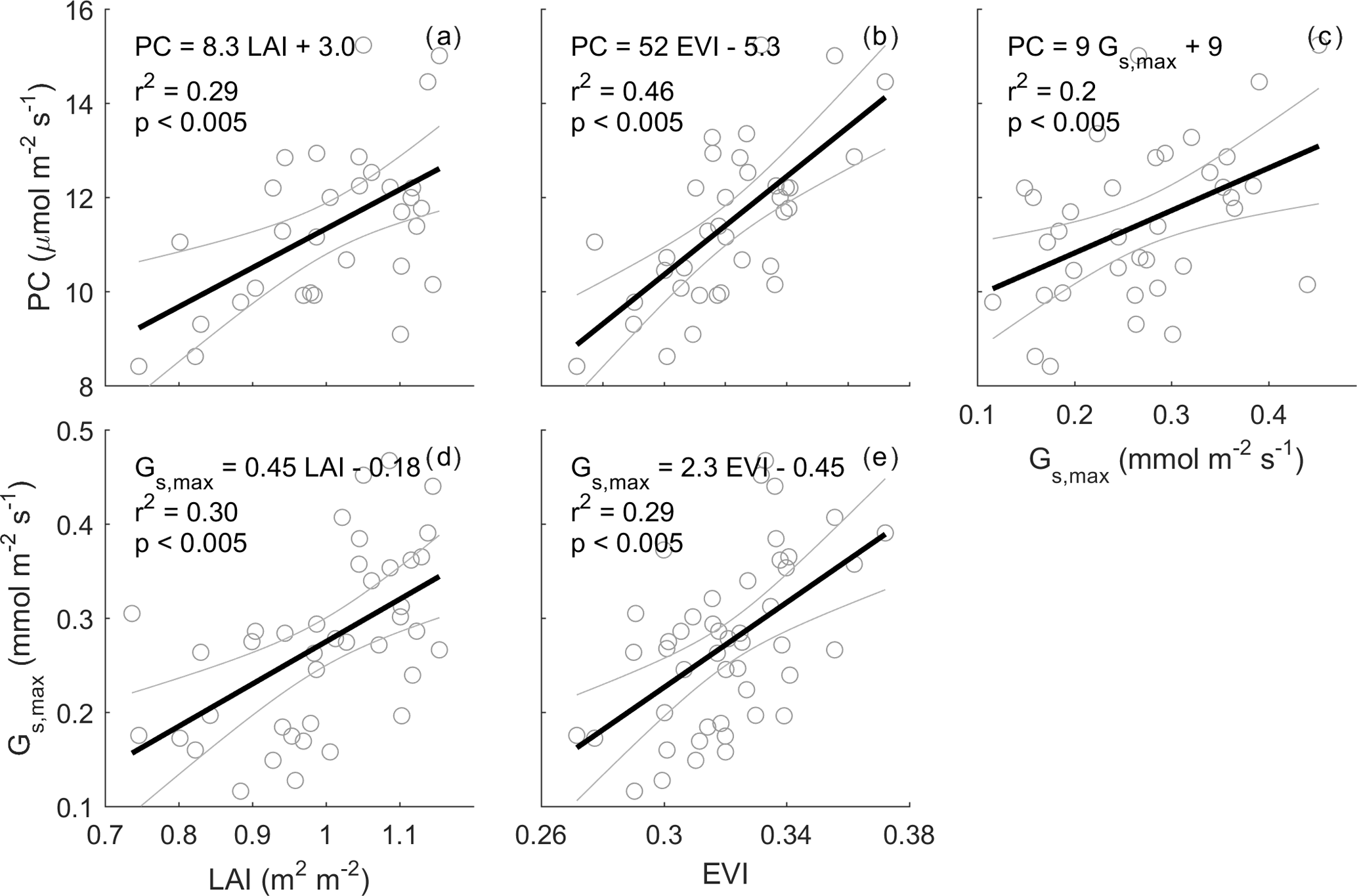
Figure 6 Relationships between monthly PC (µmol m⁻² s⁻¹), LAI (m² m⁻²), enhanced vegetation index (EVI) and maximum surface conductance (G_s,max). Monthly PC and monthly G_s,max are calculated as the median of half-hourly GPP and half-hourly G_s when PPFD is 800–1200 µmol m⁻² s⁻¹ and D is 1–1.5 kPa; rain events are filtered for G_s,max estimation to minimise evaporation contribution to evapotranspiration (see Sect. 2). Monthly LAI is calculated as mean of LAI smoothed by a spline. Thick black line shows a linear regression. For PC calculation, GPP data are only used when quality-checked NEE is available (GPP = NEE measured − ER estimated by a neural network; see Sect. 2).

3.6 Canopy phenology control of GPP

Monthly average photosynthetic capacity (PC) varied by a factor of ∼ 2 across the study period, ranging from 8.4 µmol m⁻² s⁻¹ before the leaf flush in November 2014 to 15 µmol m⁻² s⁻¹ after the leaf flush occurred in March 2016. We expected that PC could be predicted by LAI, EVI and G_s. Leaf area index (LAI) and photosynthetic capacity (PC) were significantly correlated; the slope was significantly different from zero (r²=0.29, p < 0.005, PC = 8.3 LAI + 3.0, Fig. 6). EVI was even more significantly correlated with PC (r²=0.46, p < 0.005, PC = 52 EVI − 5.3, Fig. 6). G_s,max was significantly correlated with PC (r²=0.2, p < 0.005, PC = 9 $G_{\mathrm{s},\max }+\mathrm{9}$) and LAI (r²=0.30, p < 0.005, $G_{\mathrm{s},\max }=\mathrm{0.45}$ LAI − 0.18), and with EVI (r²=0.29, p < 0.005, $G_{\mathrm{s},\max }=\mathrm{2.3}$ EVI − 0.45). The correlations with NDVI were less significant than with EVI (see Fig. S9).

4 Discussion

We measured four consecutive years of carbon, water and energy fluxes in a native evergreen broadleaf eucalyptus forest, including canopy dynamics and environmental drivers (photosynthetically active radiation, air and soil temperature, precipitation, soil water content and atmospheric demand). We hypothesised that the Cumberland Plain forest would be a carbon sink all year-round, similar to other eucalypt forests (Beringer et al., 2016; Hinko-Najera et al., 2017; Keith et al., 2012). We also hypothesised higher net carbon uptake during summer, due to warmer temperatures, higher light and longer day length contributing to higher photosynthesis, compared to winter. However, the site was a net source of carbon during summer, and a net sink of carbon during winter.

The seasonal pattern of NEE was driven mostly by ER, as the seasonal amplitude of ER was larger than the seasonal amplitude of GPP. The seasonality of ER may be explained by the positive effects of higher temperatures on the rates of autotrophic respiration (Tjoelker et al., 2001), and on the activity of microbes to increase soil organic matter decomposition (Lloyd and Taylor, 1994); low soil moisture in the shallow layers sometimes limited decomposition (January and February 2014, January and December 2015, February and December 2017; see Fig. 1), but often regular rainfall maintained adequate soil moisture. The relatively low seasonality of GPP may be partly explained by lower photosynthetic capacity in early summer (before January) when LAI was at its lowest, and the canopy reached maximum age because new leaves had not yet emerged. The ER-driven seasonality of NEE is in sharp contrast with cool-temperate forests where GPP drives the seasonality of NEE. ER-driven NEE seasonality was also observed in an Asian tropical rain forest, as ER was higher than GPP in the rainy season leading to net ecosystem carbon loss, while in the dry season, ecosystem carbon uptake was positive (Zhang et al., 2010). This pattern was also observed in an Amazon tropical forest (Saleska et al., 2003).

A strong morning–afternoon hysteresis of NEE response to PPFD occurred in summer, and less so in winter (Fig. 3). In winter, low D and moderately warm daytime air temperatures and high PPFD were sufficient to maintain high photosynthesis rates throughout most of the day (Fig. 1). In summer, two possible explanations of the diurnal hysteresis of NEE include (1) ER is greater in the afternoon compared to morning and (2) GPP is lower in the afternoon compared to morning. Explanation (1) is plausible, as temperature drives autotrophic and heterotrophic respiration; however, it is unlikely to explain the hysteresis magnitude which is higher in summer compared to winter. Explanation (2) could arise from lower afternoon stomatal conductance or lower photosynthetic capacity (e.g. the maximum rate of carboxylation, Vcmax, decreases at high T_a), or a combination of both, or even circadian regulation (Jones et al., 1998; Resco de Dios et al., 2015). An analysis of surface conductance showed strong stomatal regulation (Figs. 2, 3, 5), induced by high atmospheric demand and high air temperature (Duursma et al., 2014), limiting photosynthesis during the afternoon of warm months (see Fig. S10). These diurnal patterns of NEE, GPP and ER play a strong role in regulating the seasonal carbon cycling dynamics in this ecosystem. A wavelet coherence analysis between D and GPP showed strong coherence at seasonal timescale (periods of 3 months); see Fig. S11.

We observed comparable responses of leaf-level and ecosystem-level gas exchange to environmental drivers (Fig. 5). The larger magnitude of A_max than GPP at low D may be explained by the proportion of shaded leaves in the ecosystem. The similar magnitude for G_s and g_s was also expected, as LAI was close to 1 and R_n was not a driver for stomatal conductance. The peaked pattern of T versus D, as opposed to the saturating pattern of ET, may be explained by (1) the contribution of soil evaporation to ET or (2) the presence of mistletoe, known for not regulating their stomata (Griebel et al., 2017). The higher magnitude of leaf water use efficiency resulted from the combination of higher A_max and similar or lower leaf transpiration compared to ET. Furthermore, we compared leaf level g₁ and ecosystem level G₁, using the optimal stomatal conductance model (Medlyn et al., 2011): G₁ was lower than g₁ (1.6 ± 0.06 for G₁, 4.4 ± 0.2 for g₁; see Fig. S12).

Our study demonstrated that canopy dynamics (specifically, LAI in our study) play an important role in regulating seasonal variations in GPP even in evergreen forests. Similar observations emerged from a tropical forest, where LAI and leaf age explained the seasonal variability of GPP (Wilson et al., 2001; Wu et al., 2016), as the photosynthetic capacity (PC, the maximum rate of GPP in optimal environmental conditions) varied with leaf age. In Australian forests, PC (A_max) of leaves was also found to decrease with leaf age: A_max decreased by 30 % on average between young and old leaves, for 10 different species (Reich et al., 2009). In the Cumberland Plain forest, periods with high LAI co-occur with mature, efficient leaves, and periods with low LAI co-occur with old, less efficient leaves. LAI was correlated with PC, which was probably the result of both a greater number of leaves and more efficient leaves. Remotely sensed vegetation indices such as EVI or NDVI assess whether the target being observed contains live green vegetation. In Australia, NDVI and EVI were good predictors of photosynthetic capacity in savanna, mulga and Mediterranean–mallee ecosystems (Restrepo-Coupe et al., 2016). For our site, EVI was a good predictor of PC, which was surprising as satellite-derived LAI values have been found to be typically inaccurate in open forests and forests in southeast Australia (Hill et al., 2006). NDVI was a poor predictor of PC (see Fig. S9).

In a global study, it was shown that mean annual NEE decreased with increasing dryness index (PET ∕ P) in sites located below 45^∘ N (Yi et al., 2010). It has also been shown that Eucalyptus grows more slowly in warm environments (Prior and Bowman, 2014). At our site, and in a previous study in eucalyptus forest (van Gorsel et al., 2013), GPP decreased with D above a threshold of ∼ 1.3 kPa. Our results indicate that surface conductance (G_s) decreased above that threshold, suggesting that the decrease in GPP is caused by stomatal regulation. As D correlates with air temperature, it is difficult to distinguish the relative contribution of D and T_a to the decrease of G_s, but they are both thought to impact G_s (Duursma et al., 2014). Cumberland Plain has the highest mean annual temperature and the highest dryness index among the four eucalyptus forest eddy covariance sites in southeast Australia (Beringer et al., 2016), which could explain its strong sensitivity to D and hence its unique seasonality.

5 Conclusions

The Cumberland Plain forest was a net C source in summer and a net C sink in winter, in contrast to other Australian eucalypt forests which were net C sinks year-round. ER drove NEE seasonality, as the seasonal amplitude of ER was greater than GPP. ER was high in the warmer, wetter months of summer, when environmental conditions supported high autotrophic respiration and heterotrophic decomposition. Meanwhile, GPP was limited by lower LAI and probably older leaves in early summer, and by high D which limited G_s throughout the summer. Despite being evergreen, there was significant temporal variation in LAI, which was correlated with monthly photosynthetic capacity and monthly surface conductance. Understanding LAI dynamics and its response to precipitation regimes will play a key role in climate change feedback.