the Creative Commons Attribution 4.0 License.
the Creative Commons Attribution 4.0 License.
 | 19 Jul 2018
Modeling seasonal and vertical habitats of planktonic foraminifera on a global scale
Lukas Jonkers
Michal Kucera
Michael Schulz
Species of planktonic foraminifera exhibit specific seasonal production patterns and different preferred vertical habitats. The seasonal and vertical habitats are not constant throughout the range of the species and changes therein must be considered when interpreting paleoceanographic reconstructions based on fossil foraminifera. However, detecting the effect of changing vertical and seasonal habitat on foraminifera proxies requires independent evidence for either habitat or climate change. In practice, this renders accounting for habitat tracking from fossil evidence almost impossible. An alternative method that could reduce the bias in paleoceanographic reconstructions is to predict species-specific habitat shifts under climate change using an ecosystem modeling approach. To this end, we present a new version of a planktonic foraminifera model, PLAFOM2.0, embedded into the ocean component of the Community Earth System Model version 1.2.2. This model predicts monthly global concentrations of the planktonic foraminiferal species Neogloboquadrina pachyderma, N. incompta, Globigerina bulloides, Globigerinoides ruber (white), and Trilobatus sacculifer throughout the world ocean, resolved in 24 vertical layers to 250 m of depth. The resolution along the vertical dimension has been implemented by applying the previously used spatial parameterization of carbon biomass as a function of temperature, light, nutrition, and competition on depth-resolved parameter fields. This approach alone results in the emergence of species-specific vertical habitats, which are spatially and temporally variable. Although an explicit parameterization of the vertical dimension has not been carried out, the seasonal and vertical distribution patterns predicted by the model are in good agreement with sediment trap data and plankton tow observations. In the simulation, the colder-water species N. pachyderma, N. incompta, and G. bulloides show a pronounced seasonal cycle in their depth habitat in the polar and subpolar regions, which appears to be controlled by food availability. During the warm season, these species preferably occur in the subsurface (below 50 m of water depth), while towards the cold season they ascend through the water column and are found closer to the sea surface. The warm-water species G. ruber (white) and T. sacculifer exhibit a less variable shallow depth habitat with highest carbon biomass concentrations within the top 40 m of the water column. Nevertheless, even these species show vertical habitat variability and their seasonal occurrence outside the tropics is limited to the warm surface layer that develops at the end of the warm season. The emergence in PLAFOM2.0 of species-specific vertical habitats, which are consistent with observations, indicates that the population dynamics of planktonic foraminifera species may be driven by the same factors in time, space, and with depth, in which case the model can provide a reliable and robust tool to aid the interpretation of proxy records.
- Article
(6551 KB) - Full-text XML
-
Supplement
(8755 KB) - BibTeX
- EndNote


Planktonic foraminifera are found throughout the open ocean, where they inhabit roughly the top 500 m of the water column (Fairbanks et al., 1980, 1982; Kohfeld et al., 1996; Kemle-von Mücke and Oberhänsli, 1999; Mortyn and Charles, 2003; Field, 2004; Kuroyanagi and Kawahata, 2004; Bergami et al., 2009; Wilke et al., 2009; Pados and Spielhagen, 2014; Iwasaki et al., 2017; Rebotim et al., 2017). Their calcareous shells, preserved in ocean sediments, are widely used to reconstruct past climate conditions. To do so, information about their habitat including their horizontal and vertical distribution is needed. It is known from observational data that the prevailing environmental conditions, such as temperature, stratification, light intensity, and food availability, affect the growth and distribution of the individual planktonic foraminifera (Fairbanks et al., 1980, 1982; Bijma et al., 1990b; Watkins et al., 1996; Schiebel et al., 2001; Field, 2004; Kuroyanagi and Kawahata, 2004; Žarić et al., 2005; Salmon et al., 2015; Rebotim et al., 2017). Based on stratified plankton tow and sediment trap data the seasonal succession of planktonic foraminifera species has been assessed on a local or regional scale (e.g., Fairbanks and Wiebe, 1980; Kohfeld et al., 1996; Wilke et al., 2009; Jonkers et al., 2013; Jonkers and Kučera, 2015), whereas for a broader regional or global perspective, modeling approaches have been used to study the seasonal variations in the surface (mixed) layer of the ocean (Žarić et al., 2006; Fraile et al., 2008, 2009a, b; Lombard et al., 2011; Kretschmer et al., 2016). Comparatively less is known about the depth habitat of planktonic foraminifera species and how it varies seasonally. Although previous studies identified different environmental and ontogenetic factors (i.a., temperature, chlorophyll a concentration, the lunar cycle, and/or the structure of the water column), which influence the species-specific depth habitats including their mean living depth and vertical migration (e.g., Fairbanks and Wiebe, 1980; Fairbanks et al., 1982; Schiebel et al., 2001; Simstich et al., 2003; Field, 2004; Salmon et al., 2015; Rebotim et al., 2017), the only attempt to model the vertical habitat is by Lombard et al. (2011).
It is well known that species-specific habitats vary seasonally and spatially depending on the prevailing climatic conditions (Mix, 1987; Mulitza et al., 1998; Ganssen and Kroon, 2000; Skinner and Elderfield, 2005; Jonkers and Kučera, 2015). Yet, despite this evidence for a variable habitat, it is often assumed in paleoceanographic studies that the habitat of planktonic foraminifera is constant, i.e., that it does not change in time and space, potentially leading to erroneous estimates of past climate conditions. Jonkers and Kučera (2017) recently highlighted how foraminifera proxies are affected by habitat tracking and showed that by not accounting for this behavior, spatial and temporal trends in proxy records may be underestimated. Given the habitat variability of planktonic foraminifera, it is more than likely that a climate-dependent offset from mean annual sea surface conditions results not only from seasonal but also from depth habitat variability due to changes in ambient conditions. Such vertical habitat variability was shown by Rebotim et al. (2017), who investigated parameters controlling the depth habitat of planktonic foraminifera in the subtropical eastern North Atlantic. In line with studies from other regions of the world ocean (e.g., Fairbanks et al., 1982; Bijma et al., 1990a; Ortiz et al., 1995; Schiebel et al., 2001; Field, 2004; Salmon et al., 2015), Rebotim et al. (2017) identified distinct species-specific depth habitats, but they also showed that the habitats vary on lunar and seasonal timescales and in response to temperature, chlorophyll a, and other environmental factors. Evidence for variable depth habitats at least on a regional scale has emerged from studies in other regions (Watkins et al., 1998; Peeters and Brummer, 2002; Kuroyanagi and Kawahata, 2004).
These observations underline the necessity to consider species-specific habitats and their variability on a global scale to increase the reliability of paleoceanographic reconstructions. However, a global assessment of species-specific depth habitat variability in time and space and the potential underlying control mechanisms is lacking. Since the observational data coverage of the global ocean is too sparse to provide in this regard a broad general estimate, we apply an ecosystem modeling approach to predict the vertical and seasonal distribution of planktonic foraminifera on a global scale.
2.1 Approach
To predict the seasonally varying global species-specific depth habitat of planktonic foraminifera, we modified the previously developed planktonic foraminifera model PLAFOM (Fraile et al., 2008; Kretschmer et al., 2016), which is implemented as an off-line module into the ocean component of the Community Earth System Model version 1.2.2 (CESM1.2; Hurrell et al., 2013), with active ocean biogeochemistry (which is denoted as the CESM1.2(BGC) configuration). This model system simulates the monthly concentrations of five modern planktonic foraminiferal species, which are widely used in paleoceanographic reconstructions. The original approach of Fraile et al. (2008) and Kretschmer et al. (2016) aimed to predict the distribution of planktonic foraminifera in the surface mixed layer on geological timescales. This model version has been successfully used to assess the effect of changing environmental conditions on species distributional patterns in time and space (Fraile et al., 2009a, b; Kretschmer et al., 2016) and to aid in interpreting paleoceanographic records regarding seasonal production shifts in the geological past (Kretschmer et al., 2016), but could not provide any information about depth. To implement the vertical dimension, we used an approach in which we first updated PLAFOM (hereafter referred to as PLAFOM2.0) by including light dependency for symbiont-bearing planktonic foraminifera and then applied the previously used spatial parameterization of carbon biomass as a function of temperature, nutrition, and competition, together with light, on depth-resolved parameter fields. By combining PLAFOM2.0 with the CESM1.2(BGC) configuration (hereafter referred to as the CESM1.2(BGC+PLA) configuration), the vertical dimension can be resolved throughout the ocean, with 24 layers in the top 250 m. Thus, PLAFOM2.0, belonging to a suite of proxy system models (e.g., Pollard and Schulz, 1994; Schmidt, 1999; Fraile et al., 2008; Evans et al., 2013; Dee et al., 2015; Völpel et al., 2017), will aid the interpretation of paleoclimate reconstructions. In addition, PLAFOM2.0 has the potential to be used in a paleoclimate data assimilation framework (see, e.g., Goosse et al., 2010; Steiger et al., 2014; Dee et al., 2016; Hakim et al., 2016).
2.2 CESM1.2(BGC) configuration
We used the CESM1.2(BGC) configuration (Moore et al., 2013; Lindsay et al., 2014) as a code base. This configuration includes the Biogeochemical Elemental Cycling (BEC) model (Moore et al., 2004, 2006; Krishnamurthy et al., 2007; Moore and Braucher, 2008), which is based on the upper ocean ecosystem model of Moore et al. (2002a, b) coupled to a biogeochemistry model based on the Ocean Carbon Model Intercomparison Project (OCMIP; Doney et al., 2006). The BEC model includes various potentially growth-limiting nutrients (nitrate, ammonium, phosphate, dissolved iron, and silicate), three explicit phytoplankton functional types (diatoms, diazotrophs, pico- and nano-phytoplankton), a partial calcifier class (representing coccolithophores), a single adaptive zooplankton class, dissolved organic matter, sinking particulate detritus, and full carbonate system thermodynamics (Moore et al., 2004, 2013). Phytoplankton growth rates are controlled by temperature, light, and available nutrients (Moore et al., 2002b, 2004). The single zooplankton pool grazes on all phytoplankton types, whereby the routing of grazed material varies depending on the type of prey (Moore et al., 2004, 2013). For further details, we refer to Moore et al. (2002b, 2004, 2013).
The BEC model has been embedded into the ocean component of CESM version 1.2.2. CESM1.2 is a fully coupled climate model consisting of several components including the atmosphere, ocean, land, and sea ice (Hurrell et al., 2013), whereby the geophysical fluxes among the components are exchanged through a central coupler (Craig et al., 2012). Here we performed an ocean-ice-only simulation with active ocean biogeochemistry, whereby the ocean model is coupled to both the sea ice model and data models for the atmosphere, land, and river routing, which provide the required input data for the simulation.
The CESM1.2 ocean component is the Parallel Ocean Program version 2 (POP2; Smith et al., 2010; Danabasoglu et al., 2012), with a zonal resolution of 1∘ and an increased meridional resolution of 0.27∘ near the Equator. POP2 employs a nonuniform dipolar grid with the North Pole being displaced into Greenland. With a total number of 60 vertical levels, the grid spacing is fine near the surface (10 levels in the top 100 m) and increases with depth to 250 m near the bottom. The sea ice component of CESM1.2 is the Community Ice Code version 4 (CICE4; Hunke and Lipscomb, 2008; Holland et al., 2012), which uses the same horizontal grid as the ocean model.
2.3 PLAFOM2.0
This new model version, PLAFOM2.0, considers the polar species Neogloboquadrina pachyderma, which is supplemented by the subpolar species N. incompta (sensu Darling et al., 2006) and Globigerina bulloides as well as by the warm-water algal symbiont-bearing species Globigerinoides ruber (white) and Trilobatus sacculifer (sensu Spezzaferri et al., 2015). Those species have been chosen as they can be considered to represent a large portion of the planktonic foraminiferal biomass in the surface ocean (for further details see Kretschmer et al., 2016). The different planktonic foraminifera species were added to the ocean component of CESM1.2 as optional passive tracers with the requirement that the BEC model is active.
PLAFOM2.0 is driven by temperature, the available food sources (including zooplankton, diatoms, small phytoplankton, and organic detritus), and also light availability, whereby the latter only matters with regard to the growth of the two algal symbiont-bearing species (Erez, 1983; Jørgensen et al., 1985; Gastrich, 1987; Gastrich and Bartha, 1988) and G. bulloides, which according to the latest findings hosts the picocyanobacterium Synechococcus as a photosynthesizing endobiont (Bird et al., 2017). Synechococcus is known to be important for cyanobacterial photosynthesis in marine and freshwater ecosystems (Ting et al., 2002; Jodłowska and Śliwińska, 2014).
Table 1Model parameters and their modifications relative to Fraile et al. (2008) and/or Kretschmer et al. (2016). The original value is given in parentheses.
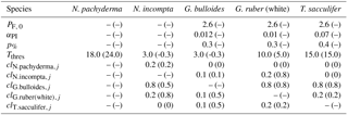
PF, 0 – maximum foraminiferal growth rate (in day−1) at 30 ∘C (derived from the maximum zooplankton growth rate at 20 ∘C given by Doney et al., 1996). αPI – initial slope of the photosynthesis–irradiance (PI) curve (in m2 W−1day−1) (derived from the PI curve of Synechococcus given in Jodłowska and Śliwińska (2014) for G. bulloides and of endosymbiotic dinoflagellates given in Jørgensen et al. (1985) for T. sacculifer). p% – fraction of photosynthesis contributing to foraminiferal growth rate. Tthres – minimum (for N. pachyderma) or maximum (for all other species) threshold temperature at which foraminiferal species can thrive (in ∘C). clij – competition pressure of species i upon species j.
The food preferences and temperature tolerance limits for each species have been derived from sediment trap data and culturing experiments (see Fraile et al., 2008, for details). Changes in the foraminifera carbon concentration for each species are determined as follows:
where F is the foraminifera carbon concentration (in mmol C m−3), GGE (gross growth efficiency) is the portion of grazed matter that is incorporated into foraminiferal carbon biomass, TG represents total grazing (i.e., the growth rate in mmol C m−3 s−1), and ML denotes mass loss (i.e., the mortality rate in mmol C m−3 s−1). To properly simulate the vertical distribution of each considered planktonic foraminifera, we included light dependency and modified parts of the parameterizations of the foraminiferal species concentration. Therefore, we extended the growth rate equation by not only considering food availability and temperature sensitivity, but also light intensity to define growth. Additionally, we adjusted parts of the mortality rate equation to improve the model accuracy. In the following, the performed modifications are described in detail in regard to growth and mortality rates. The modifications compared to the earlier model version are summarized in Table 1.
2.3.1 Growth rate
The growth rate depends on the available food and temperature sensitivity of each foraminiferal species as well as on light for the species with algal symbionts and/or cyanobacterial endobionts. To account for the light dependence with depth influencing the growth of G. bulloides and of the spinose species G. ruber (white) and T. sacculifer, we included a photosynthetic growth rate. As a first-order estimate, we applied a similar approach as Doney et al. (1996) and Geider et al. (1998), who determined phytoplankton growth rates based on available light and nutrient conditions, which have been accordingly used in the BEC model (Moore et al., 2002b, 2004). We are aware that a phytoplankton response to light is not directly transferable to planktonic foraminifera, but we argue that as a first approximation this is a valid approach.
Photosynthesis depends on light availability and temperature. This codependency can be expressed as follows:
where PF, photo is the foraminiferal specific rate of photosynthesis (in s−1) and PF, max is the maximum value of PF, photo at temperature T (in s−1) calculated as
αPI is the initial slope of the photosynthesis–irradiance curve (in m2 W) (Table 1), IPAR is the average irradiance over the mixed layer depth provided by the ecosystem model (in W m−2), PF, 0 represents the maximum foraminiferal growth rate at a specific temperature T0 (in s−1) (Table 1), and Tfunc is the temperature response function (dimensionless). The temperature function is defined as
with a q10 value of 1.5 (Sherman et al., 2016), T being the ambient ocean temperature (in K), and T0 the reference temperature of 303.15 K.
The photosynthetic growth rate, PF (in mmol C m−3 s−1), can finally be determined as follows:
where p % represents the fraction of photosynthesis contributing to growth (see Table 1).
2.3.2 Mortality rate
The mortality rate is determined by respiration loss, predation by higher trophic levels, and competition among species. To improve the seasonal patterns in the foraminiferal carbon biomass for low temperatures, we followed Moore et al. (2004) and adjusted the temperature dependence of the predation term (MLpred in mmol C m−3 s−1):
where fmort2 represents the quadratic mortality rate (in s−1(mmol C m−3)−1), Tfunc is the temperature response function (dimensionless) used for scaling, and Fp (in mmol C m−3) is used to limit the planktonic foraminifera mortality at very low carbon biomass levels. Compared to Fraile et al. (2008), here predation is scaled by Eq. (2), a temperature function using a q10 value of 1.5 (Sherman et al., 2016).
Additionally, we included a stronger competitive behavior of G. bulloides by adjusting the free parameters in the competition term. In PLAFOM2.0, competition (MLcomp in mmol C m−3 s−1) is defined as follows:
with Fi being the concentration of the foraminiferal species exerting competition, clij the maximum competition pressure of species i upon species j, and d the constant controlling the steepness of the Michaelis–Menten relationship for competition. In comparison with Kretschmer et al. (2016), we only modified the parameter clij for N. incompta, G. bulloides, and G. ruber (white) (Table 1).
We added the present implementation of PLAFOM2.0 to the code trunk of POP2 as a separate module. Additionally, the food sources for the planktonic foraminifera species are computed in the ecosystem model and instantly passed to PLAFOM2.0 to calculate the foraminifera carbon concentration. A parameter sensitivity assessment for PLAFOM was carried out by Fraile et al. (2008) and since PLAFOM2.0 is based on the same underlying formulation, we consider an extensive new sensitivity assessment not essential at this stage. For a more detailed description of the planktonic foraminifera model and its behavior on a regional or global scale in the surface mixed layer, we refer to Fraile et al. (2008) and Kretschmer et al. (2016).
2.4 Model simulation
To test the model, we performed a preindustrial control experiment. Therefore, we derived the initial ocean and sea ice states from an ocean-ice-only simulation, which did not include the BEC ocean biogeochemistry. This model integration was spun up from rest for 300 years to approach a quasi-steady state by using a climatological forcing (based on atmospheric observations and reanalysis data) as repeated normal year forcing. Heat, freshwater, and momentum fluxes at the sea surface are based on the atmospheric data sets developed by Large and Yeager (2004, 2009) and implemented following the CORE-II protocol (Coordinated Ocean-ice Reference Experiment) suggested by Griffies et al. (2009).
The oceanic and sea ice tracer fields (such as potential temperature, salinity, and ice area) resulting from the end of this 300-year-long spin-up run were used to initialize the CESM1.2(BGC+PLA) preindustrial control simulation. The biogeochemical tracer fields (such as nutrients) were, i.a., initialized from climatologies. For instance, initial nutrient (phosphate, nitrate, silicate) distributions were taken from the World Ocean Atlas 2009 (WOA09; Garcia et al., 2010), initial values for dissolved inorganic carbon and alkalinity are from the Global Ocean Data Analysis Project (GLODAP; Key et al., 2004), and zooplankton, phytoplankton pools, and dissolved organic matter have been initialized uniformly at low values (Moore et al., 2004). Additionally, each planktonic foraminiferal species was also initialized uniformly at low values assuming the same (vertical) distribution as the zooplankton component of the BEC model. Furthermore, the atmospheric deposition of iron and dust is based on the climatology of Luo et al. (2003).
The CESM1.2(BGC+PLA) preindustrial control simulation was integrated for 300 years to reach stable conditions in the ocean biogeochemistry in the upper 500 m of the water column (see Fig. S1 in the Supplement). Since this simulation has been forced and/or initialized based on climatologies, interannual variability and forcing trends can be excluded, and therefore we focus our analysis on the model output of only one year, here year 300.
2.5 Comparison to observations
To validate the model performance, we compare the simulated spatial and temporal distributions of the considered planktonic foraminiferal species with data from core tops, sediment traps, and plankton tows (Fig. 1). Based on data availability, we focus our analysis on distinct regions distributed over the world ocean covering all climate zones from the poles to the tropics.
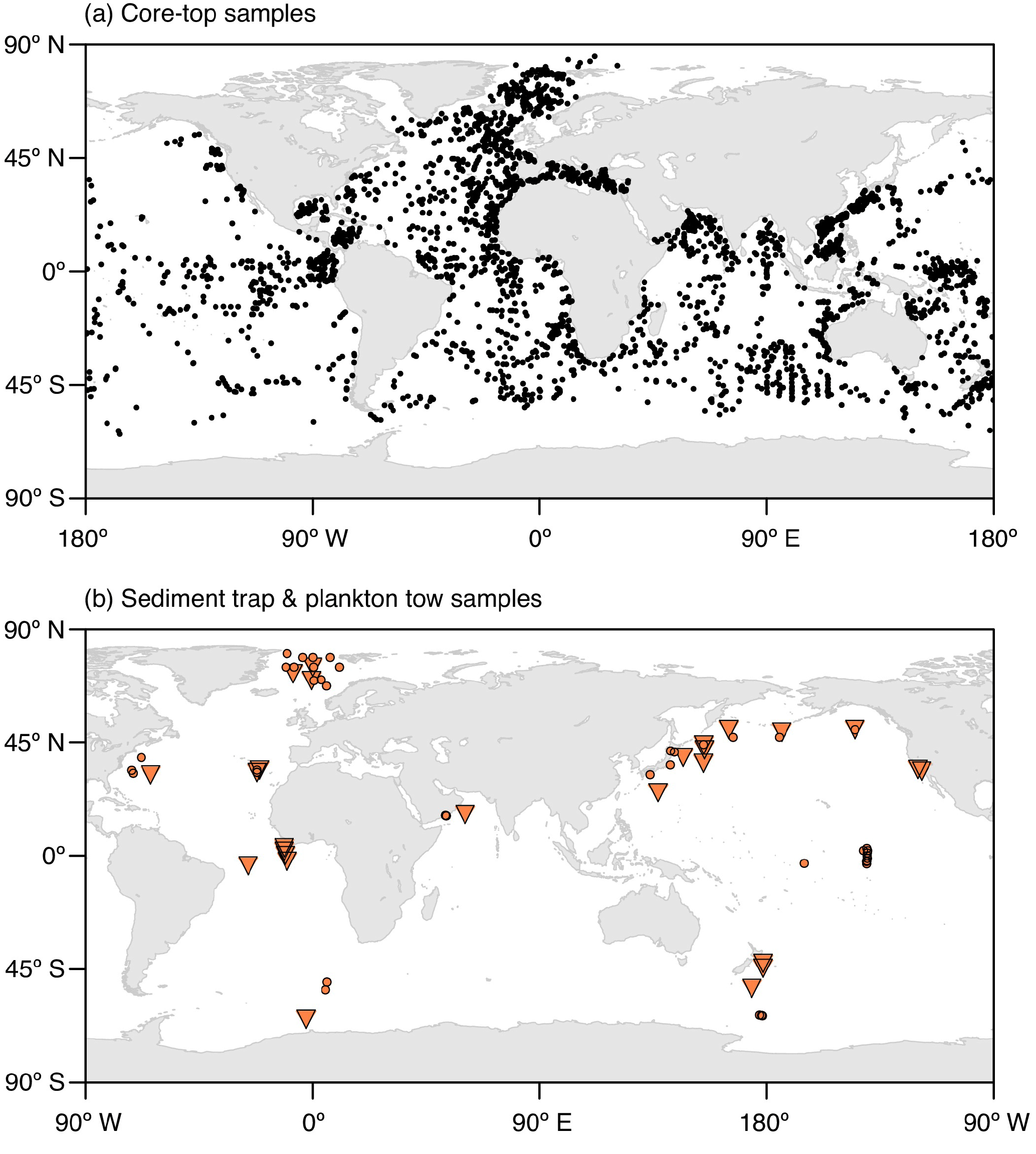
Figure 1Locations of (a) the core-top samples with planktonic foraminifera counts and (b) the plankton tow (orange circles) and sediment trap (orange triangles) samples used for the model validation. The map in Fig. 1a shows a combination of the data sets of Prell et al. (1999), Pflaumann et al. (1996, 2003), and Kucera et al. (2005). The respective information on the sediment trap and plankton tow data shown in Fig. 1b is given in Tables S1 and S2 in the Supplement.
2.5.1 Core-top data
To examine the spatial pattern of the five considered planktonic foraminiferal species, we compared the model predictions with fossil data by using in total 2896 core-top samples distributed over all oceans (Fig. 1a). We combined the Brown University Foraminiferal Database (Prell et al., 1999) with the data assembled by the MARGO project (Kucera et al., 2005) and the data sets provided by Pflaumann et al. (1996, 2003). For the comparison, we recalculated the relative abundances of the faunal assemblages by only considering those five species used in PLAFOM2.0. Similarity between the simulated and observed abundances was quantified using the Bray–Curtis index of similarity (bjk in %) between the relative abundances of the core-top data and the modeled data at the respective sample locations.
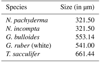
Here xji and xki are the modeled and observed relative abundances (with values between 0 and 1) of each species i at the given core-top locations, respectively. Note that for the calculation of the modeled relative abundances, we accounted for the different sizes of each individual species by multiplying the modeled annual mean concentration of each species with an estimate of their relative sizes (Table 2).
2.5.2 Sediment trap data
To compare modeled and observed seasonal production patterns, several sediment traps (Table S1, Fig. 1b) have been examined. Those can provide foraminiferal shell fluxes continuously collected over several months or even years. However, some sediment traps comprise only a few months (i.e., less than a year) and might have just recorded local short-term processes of a particular season or year and thus cannot provide a long-term and/or climatological mean.
Here we use the same approach as in Jonkers and Kučera (2015) and present the observed fluxes for multiple years from every location on a log10 scale versus day of year, whereby the zero fluxes have been replaced by half of the observed minimum flux to visualize the results. In this way, we can directly compare the peak timings of the measured fluxes at each location with the model, whereby we assume that the flux through the water column (in no. m−2 day−1) is proportional to the volume-integrated model concentrations (in mmol C m−3).
2.5.3 Plankton tow data
To analyze the vertical distribution, plankton net hauls from different sites distributed across the world ocean (Table S2, Fig. 1b) have been used for a comparison with the simulated vertical distributions. Plankton tow samples have been collected by means of a multiple opening–closing net with a vertical resolution differing between 5 depth levels (one haul) and up to 13 depth levels (two or more consecutive hauls) resolving the upper hundreds of meters of the water column. Since the plankton tow data have been collected during a particular time (i.e., a specific day or month; Table S2), the same month has been considered for the simulated vertical planktonic foraminifera profile for the model–data comparison.
Table 2Relative sizes of the analyzed planktonic foraminifera species based on estimates of species size ranges from Schmidt et al. (2004) averaged over the sample locations in that study.
Here we followed the same approach as Rebotim et al. (2017) and calculated an average living depth (ALD) and the vertical dispersion (VD) around the ALD to provide a direct comparison with the modeled depth profile. The ALD (in m) is defined as follows:
with Ci being the foraminiferal species concentration (in no. m−3) in the depth interval Di and VD (in m) is calculated as
For further information, we refer to Rebotim et al. (2017).
3.1 Modeled horizontal distribution patterns
The modeled global spatial distribution patterns based on the depth-integrated annual mean relative abundances of the five considered foraminiferal species (Fig. 2) correspond to the five major provinces of the modern ocean (i.e., polar, subpolar, transitional, subtropical, and tropical) known to be inhabited by those species (Bradshaw, 1959; Bé and Tolderlund, 1971; Hemleben et al., 1989; Kucera, 2007). Note that since the core-top data used for comparison provide information neither on the depth habitat of the planktonic foraminiferal species nor on their life cycle, the modeled annual mean relative abundances have been obtained by integrating the individual foraminiferal concentrations over the whole water column and by subsequently calculating the percentage of each species relative to the modeled total foraminiferal carbon biomass, whereby we also accounted for the different sizes of each species (Table 2).

Figure 2(a) Bray–Curtis index of similarity (in %) between the relative abundances of the modeled and core-top data as well as relative abundances of the depth-integrated modeled annual mean concentration (pale-colored contours; in % carbon biomass) and of the core-top samples (circles; in % individuals) for (b) N. pachyderma, (c) N. incompta, (d) G. bulloides, (e) G. ruber (white), and (f) T. sacculifer. The relative abundances consider only the five foraminiferal species included in PLAFOM2.0. In addition, to account for the different sizes of each foraminiferal species, we multiplied the modeled annual mean concentration of each species with their relative size (Table 2) and subsequently calculated the depth-integrated species annual mean concentrations relative to the total modeled foraminiferal carbon biomass. Note that we are aware that for a small number of core-top samples the relative abundances of the individual planktonic foraminiferal species are overestimated due to recalculations only considering N. pachyderma, N. incompta, G. bulloides, G. ruber (white), and T. sacculifer rather than the whole assemblage. However, the overall general pattern does not change and can thus be used for the model–data comparison.
For a direct comparison of the observed (i.e., the core-top data) and modeled foraminiferal community composition the Bray–Curtis index of similarity was used. The comparison reveals generally a good fit between the simulated and sedimentary assemblage composition with a median Bray–Curtis similarity of ∼68 %. The fit is particularly good in the high latitudes and in the tropics (Bray–Curtis similarity >80 %) and only a few regions (off South America and southern Africa, in the equatorial and North Pacific, and in the eastern North Atlantic) reveal a poorer agreement with similarities of <50 % (Fig. 2a).
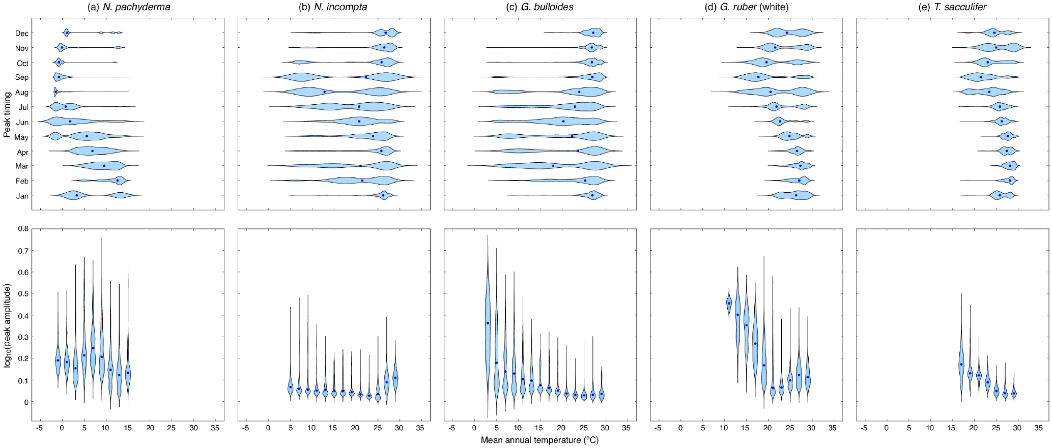
Figure 3Violin plots showing the dependence of the modeled peak timing (top row) and/or the modeled peak amplitude (bottom row) on the annual mean temperature (in ∘C) averaged over the top 55 m of the water column for (a) N. pachyderma, (b) N. incompta, (c) G. bulloides, (d) G. ruber (white), and (e) T. sacculifer. The blue dots represent the respective median values. The modeled peak timing is given in months and the modeled peak amplitude has been log transformed. Note that the peak timings of each species from the Southern Hemisphere have been transformed to Northern Hemisphere equivalents by adding or subtracting 6 months.
In the simulation, the cold-water species N. pachyderma is confined to the high latitudes dominating the polar waters of both hemispheres. Neogloboquadrina pachyderma shows the highest modeled annual mean relative abundances (>90 %) north of the Arctic Circle and south of the Antarctic Convergence, whereas toward the subtropics the species occurrence in the model is reduced gradually (Fig. 2b). Neogloboquadrina incompta occurs mainly in the subpolar to transitional water masses of the world ocean in the simulation. This species shows the highest modeled annual mean relative abundances in the latitudinal belt at around 45∘ N and/or 45∘ S (Fig. 2c). Globigerina bulloides also occurs in the subpolar to transitional waters of the world oceans with the highest modeled annual mean relative abundances (>60 %) occurring in the Southern Ocean and in the subpolar gyres (Fig. 2d). In the upwelling region of the equatorial Pacific and in the coastal upwelling systems associated with the cold eastern boundary currents of the Atlantic and Pacific oceans, G. bulloides is found with modeled annual mean relative abundances of <40 %. In the simulation, the warm-water species G. ruber (white) is mostly confined to the subtropical and tropical regions of both hemispheres, whereby the highest modeled annual mean relative abundances of up to 60 % are reached in the subtropical gyres (Fig. 2e). The lowest modeled annual mean relative abundances can be found in the ocean's upwelling areas, especially in the equatorial Pacific cold tongue, where G. ruber (white) appears to be almost absent. The modeled distribution pattern of T. sacculifer is limited to the warm waters of the subtropics and tropics and is similar to the one of G. ruber (white). Trilobatus sacculifer shows the highest modeled annual mean relative abundances (>60 %) in the equatorial Pacific between 15∘ N and 15∘ S and exhibits low modeled annual mean relative abundances (<30 %) in the coastal upwelling regions of the ocean basins (Fig. 2f).
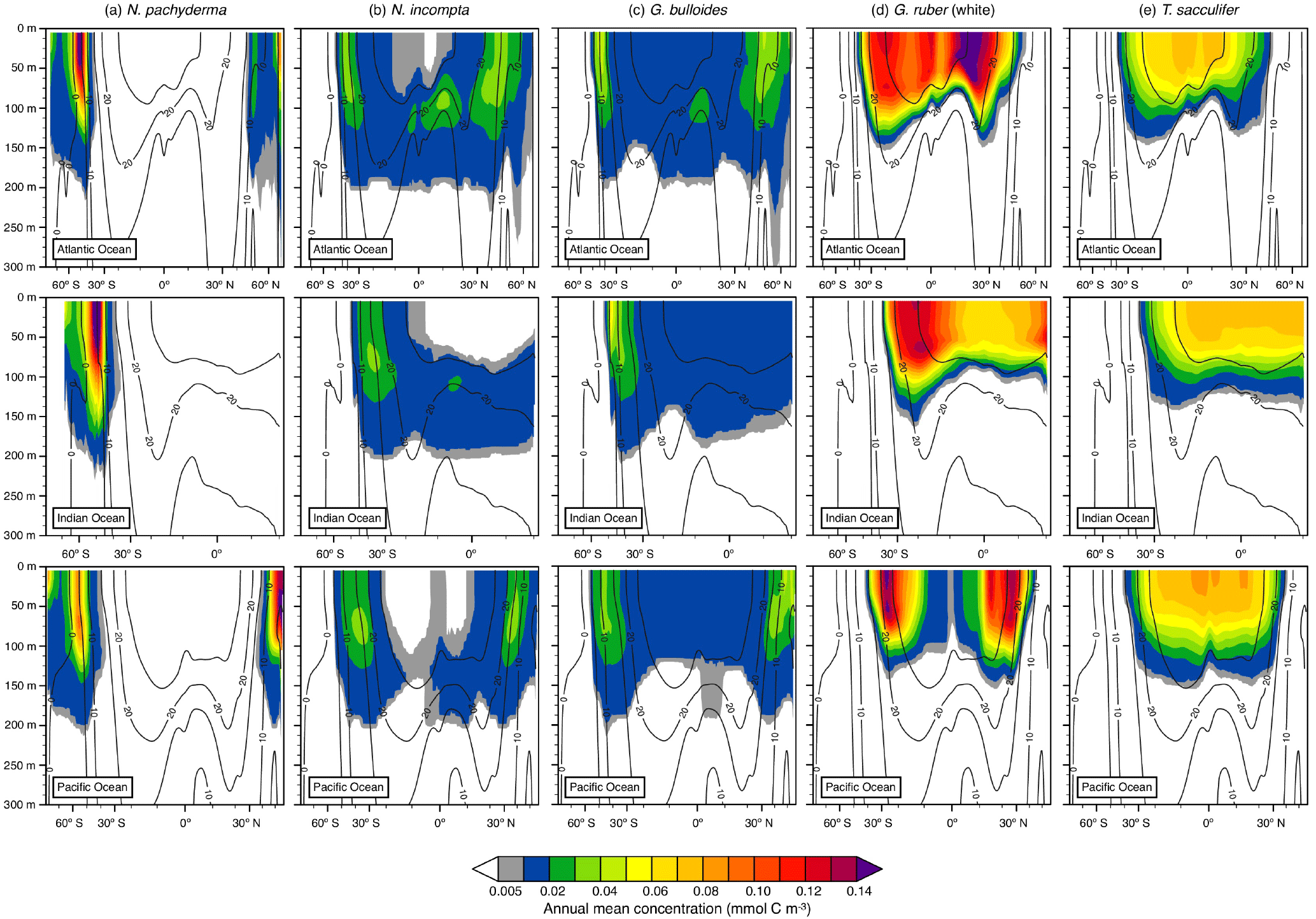
Figure 4Depth transects of the modeled annual mean concentration (in mmol C m−3) along ∼27∘ W in the Atlantic Ocean (top row), ∼71∘ E in the Indian Ocean (middle row), and ∼162∘ W in the Pacific Ocean (bottom row) over the top 300 m for (a) N. pachyderma, (b) N. incompta, (c) G. bulloides, (d) G. ruber (white), and (e) T. sacculifer. The black contour lines indicate the annual mean temperature estimates (in ∘C). The blank areas denote where a species is absent.
3.2 Modeled seasonal distribution
For each foraminiferal species, the month of modeled maximum production changes on average with temperature and consequently with latitude (Fig. 3, Fig. S2). In the simulation, there is a general tendency for the maximum production peak of the cold-water species N. pachyderma to occur later in the year (i.e., during summer) for lower annual mean temperatures (Figs. 3a and S2a). With increasing mean annual temperatures, however, the modeled peak timing occurs earlier in the year (i.e., during spring) (Fig. 3a). For N. incompta, modeled maximum production is reached during late summer in the midlatitudes at lower temperatures and is shifted towards spring and/or early summer when temperatures increase (Fig. S2b). In the low latitudes at high temperatures, however, N. incompta exhibits a constant flux pattern throughout the year (Fig. 3b). The modeled peak timing of G. bulloides is similar to the modeled peak timing of N. incompta, and the highest modeled fluxes are reached later (earlier) in the year in the midlatitudes at lower (higher) temperatures (Fig. S2c). In the warm waters (of the tropics), G. bulloides exhibits year-round a rather uniform flux pattern (Fig. 3c). In the model, both N. incompta and G. bulloides show indications of a double peak in their timing that is shifted towards the first half of the year when temperatures rise (Fig. 3b and c). This earlier-when-warmer pattern is also indicated in the modeled peak timing of N. pachyderma (Fig. 3a). Globigerinoides ruber (white) shows a uniform flux pattern year-round in the warm waters of the world ocean in the subtropical–tropical regions (Fig. S2d). In colder waters (e.g., towards higher latitudes), modeled peak fluxes of G. ruber (white) are reached in late summer and/or fall (Fig. 3d). A similar seasonal pattern in the modeled peak timing is evident for the tropical species T. sacculifer with constant fluxes occurring year-round at high temperatures in the low latitudes (Fig. S2e). At lower ambient temperatures, modeled peak fluxes of T. sacculifer occur during fall (Fig. 3e). For both G. ruber (white) and T. sacculifer, the modeled peak timing is shifted to later in the year when the surroundings become colder (Fig. 3d and e).
To allow for a global comparison of the modeled and observed flux seasonality, we standardized peak amplitudes for each foraminiferal species, i.e., the species maximum concentration divided by its annual mean. This reveals that the timing of the modeled foraminiferal peak abundances varies with temperature, but all five species exhibit an almost constant peak amplitude in their preferred thermal habitat. Outside their preferred living conditions, modeled peak amplitudes considerably increase for most of the species (Fig. 3), and thus the species experience a strong deviation from their annual mean living conditions and likely occur only at times when the ambient conditions are (close to) their optima. For the warm-water species G. ruber (white) and T. sacculifer, peak amplitudes rise when the ambient temperatures fall below 20 ∘C (Fig. 3d and e). The peak amplitude of G. bulloides increases noticeably with mean annual temperatures falling below 10 ∘C (Fig. 3c). By contrast, when ambient temperatures exceed 25 ∘C, the peak amplitude of N. incompta increases (Fig. 3b). For the cold-water species N. pachyderma, the relation between peak amplitudes and mean annual temperatures is more complex (Fig. 3a).
3.3 Modeled vertical distribution
Among the three major ocean basins, the modeled vertical distribution of each considered planktonic foraminiferal species shows similar patterns in the annual mean (Fig. 4). The temperate to cold-water species (i.e., G. bulloides, N. incompta, and N. pachyderma) occur from the surface down to about 200 m of water depth (Fig. 4a, b, and c). Neogloboquadrina pachyderma is consistently present in the top few hundred meters of the water column in the high latitudes and absent in the subtropical–tropical regions. In the polar waters of the three ocean basins, modeled maximum annual mean concentrations are found at the surface and deeper toward lower latitudes. The highest modeled annual mean concentrations of N. pachyderma are, however, located in the subpolar gyres between 0 and 75 m of water depth (Fig. 4a). Neogloboquadrina incompta is in general present between 60∘ N and 60∘ S with the modeled annual mean concentration reaching its maximum at around 100 m of water depth. In the middle to higher latitudes, N. incompta is found from the surface to ∼200 m of water depth in the Atlantic, Indian, and Pacific oceans, but seems to be rarely present in the respective uppermost water layers (i.e., between 0 and ∼75 m) of the tropics. However, the modeled annual mean concentration increases with depth, especially from the subpolar regions toward the Equator (Fig. 4b). As for N. incompta, G. bulloides has been consistently found from the surface to ∼200 m of water depth between about 60∘ N and 60∘ S (Fig. 4c). Depending on the ocean basin, modeled maximum annual mean concentrations of G. bulloides are either mainly reached at the surface (i.e., in the Indian and Pacific oceans) or at depth (i.e., in the Atlantic Ocean), but also at around 100 m of water depth in the subpolar regions of the three chosen transects. Both N. incompta and G. bulloides show the highest modeled annual mean concentrations between 30 and 60∘ latitude (Fig. 4b and c).
The warm-water species G. ruber (white) and T. sacculifer are found between the surface of each ocean basin and ∼100 m of water depth, thus occurring in a shallower depth range compared to N. pachyderma, N. incompta, and G. bulloides (Fig. 4d and e). Among all five planktonic foraminiferal species, G. ruber (white) exhibits on average the highest modeled annual mean concentrations along the transects (Fig. 4). This species is confined to the subtropical–tropical regions of the ocean basins with the highest modeled annual mean concentrations occurring between ∼15 and 30∘ latitude and the lowest around the Equator (Fig. 4d). Along the three chosen transects, modeled maximum annual mean concentrations of G. ruber (white) are almost consistently reached at the surface in the low latitudes and at around 60 m of water depth in areas where the highest modeled abundance of this species occurs. Trilobatus sacculifer also occurs predominantly between 30∘ N and 30∘ S with modeled annual mean concentrations gradually decreasing with depth. Compared to the other planktonic foraminiferal species, T. sacculifer exhibits a rather uniform distribution pattern along the different transects (Fig. 4e) with modeled maximum annual mean concentrations being primarily located at the surface.
3.4 Modeled seasonal variability of habitat depth
In the model, the depth of maximum production of each considered planktonic foraminifera changes over the course of a year (Fig. 5). Towards higher latitudes, N. incompta and N. pachyderma show maximum abundances at lower depth levels compared to low and midlatitudes. In the polar regions, N. pachyderma occurs close to the surface during winter and descends through the water column from spring to summer with modeled maximum abundances being reached at ∼40 m of water depth in summer. In the subpolar regions, N. pachyderma is generally found between 50 and 100 m of water depth for almost the entire year except for the winter season when the highest modeled concentrations are reached close to the surface (Fig. 5a). The modeled depth habitat of N. incompta increases from spring to summer and is shallower in winter in the subpolar regions (Fig. 5b). In the subtropics and tropics, however, N. incompta shows the highest modeled concentrations year-round consistently below 90 m of water depth.
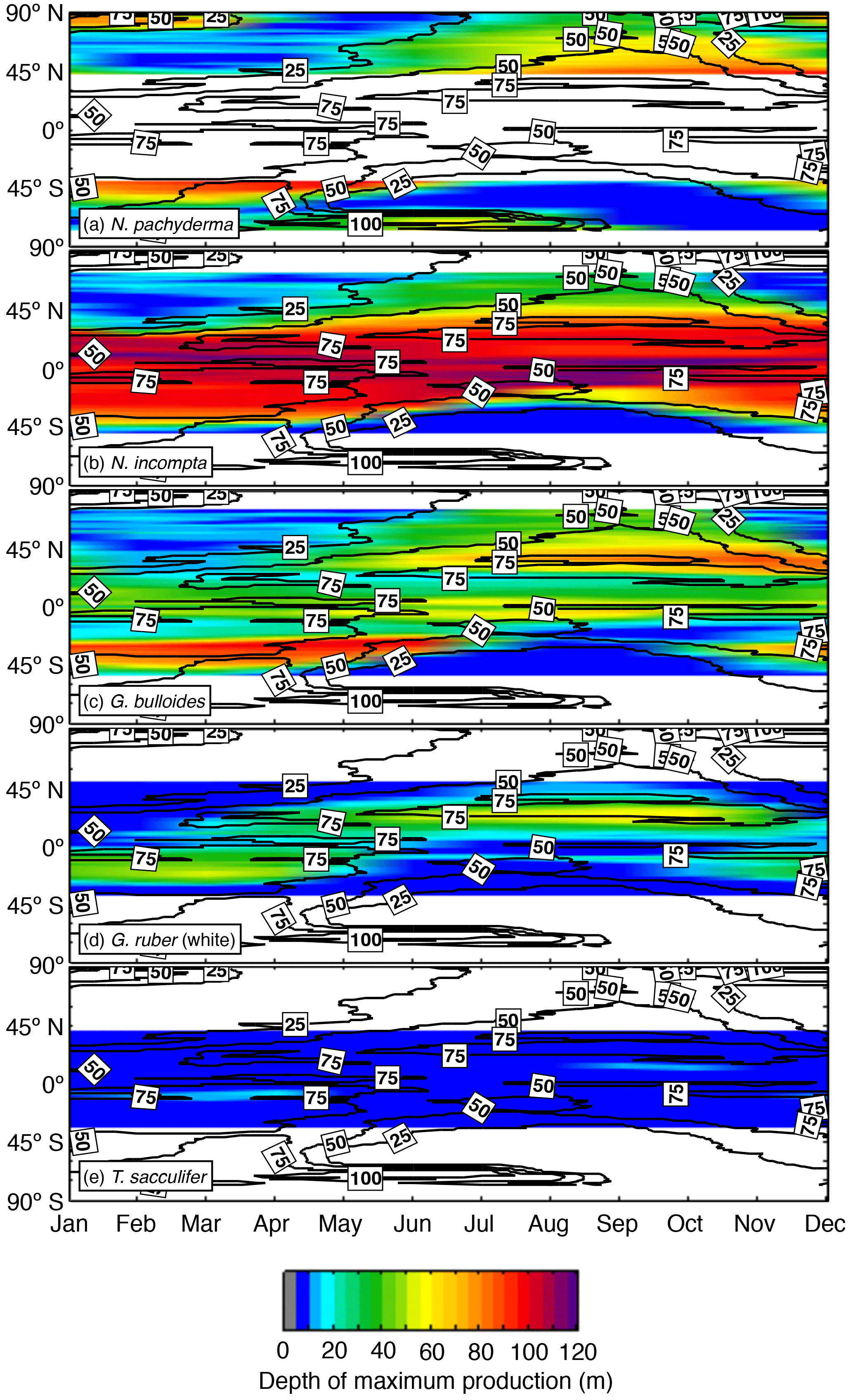
Figure 5Zonal average of the depth (in m) at which the modeled maximum production of (a) N. pachyderma, (b) N. incompta, (c) G. bulloides, (d) G. ruber (white), and (e) T. sacculifer occurs over time. The black contour lines indicate the zonal average of the (seasonally varying) depth of the chlorophyll maximum (in m). The blank areas denote where a species is absent.
Globigerina bulloides exhibits a relatively shallow habitat (i.e., up to ∼50 m of water depth) along the Equator throughout the year (Fig. 5c). In the subpolar regions, the depth of the modeled maximum production of G. bulloides varies seasonally and, similar to N. incompta, is shallower during winter and deepest during summer. The modeled depth habitat of G. ruber (white) is mostly confined to the top 60 m of the water column and seems to be less variable compared to the temperate and cold-water species (Fig. 5). In the midlatitudes and near the Equator, the highest modeled concentrations of G. ruber (white) occur close to the surface during almost the entire year, whereas in the subtropical–tropical regions, this species is most abundant below 20 m and shows a weak seasonal cycle, occurring deeper in late summer and/or early fall (Fig. 5d). Trilobatus sacculifer exhibits the least variable depth habitat in the simulation among the five considered species and is consistently found close to the surface above 20 m of water depth throughout the year (Fig. 5e).
4.1 Large-scale patterns
4.1.1 Geographical range of planktonic foraminifera species
The predicted global distribution patterns of the five considered planktonic foraminiferal species are in good agreement with the core-top data (Fig. 2a). This is remarkable considering the simplifications that had to be used to facilitate the comparison, such as the use of a constant biomass to size scaling within a species and a constant size scaling among the species.
Neogloboquadrina pachyderma is most abundant in the polar–subpolar waters of the Northern Hemisphere and Southern Hemisphere both in the model and in the core-top samples (Fig. 2b). This cold-water species dominates the waters north of the Arctic Circle and south of the Antarctic Convergence with relative abundances exceeding 90 % and is very rarely found in subtropical–tropical waters, which is also seen in the model output. Bé (1969), Bé and Tolderlund (1971), and Bé and Hutson (1977) showed that N. pachyderma mainly occurs in regions with sea surface temperatures (SSTs) below 10 ∘C, but is also present in the cold–temperate waters of, e.g., the subpolar gyres with relative abundances being reduced to 30–50 %. Thus, in areas influenced by warmer waters the abundance of this species decreases gradually. This is especially evident in the eastern North Atlantic Ocean, where the abundance of N. pachyderma is reduced to about 50 % due to the influence of the warm Atlantic Water, which is transported northward by the North Atlantic Current (NAC) (Husum and Hald, 2012). In line with the observations, the modeled annual mean relative abundances of N. pachyderma also decrease with decreasing latitude and are hence reduced towards warmer surface waters (Fig. 2b). Additionally, PLAFOM2.0 is able to reproduce the observed species abundance pattern in the North Atlantic with a reduced relative abundance of < 30 % in the area, which is influenced by the NAC. Similar to PLAFOM (see Fraile et al., 2008) a slight deviation between the simulated and observed relative abundances of N. pachyderma at the edge of the species distribution pattern is observed in the Northern Hemisphere. It has been shown that distinct genotypes discovered within this morphologically defined species exhibit different ecological preferences (Darling et al., 2006; Morard et al., 2013). Thus, the abovementioned minor discrepancy might partly arise due to the underlying model parameterizations, which are mainly based on the environmental preferences (i.e., temperature tolerance limits) of the N. pachyderma genotypes found in the Southern Ocean (for more details see Fraile et al., 2008), which differ genetically from the genotypes found in the North Atlantic and North Pacific oceans (Darling et al., 2004, 2006, 2007).
The modeled global distribution patterns of N. incompta and G. bulloides agree to a broad extent with the observations (Fig. 2c and d). Both species are predominantly found in the subarctic, subantarctic, and transitional waters of the world oceans (with relative abundances >50 %), where SSTs range between 10 and 18 ∘C (Bé and Tolderlund, 1971; Bé and Hutson, 1977). They are also highly abundant in the cool eastern boundary currents off Africa and South America (e.g., Bé and Tolderlund, 1971; Giraudeau, 1993; Darling et al., 2006) as well as in the eastern North Atlantic and occur continuously in a subantarctic belt between 30∘ S and the Antarctic Convergence (Bé, 1969; Bé and Tolderlund, 1971; Boltovskoy et al., 1996). In addition, high abundances (> 40 %) of N. incompta have been observed in the equatorial Pacific upwelling system and of G. bulloides in the Arabian Sea. In the model, N. incompta is confined to the subpolar belts at around 45∘ latitude, which matches the general distribution pattern seen in the core-top data, but the relative abundance is underestimated (here N. incompta accounts for < 20 % of the modeled assemblage compared to up to 50 % in the observations; Fig. 2c). The model prediction for G. bulloides shows, in accordance with the core-top samples, higher abundances in the subantarctic belt (here the species accounts for up to 80 % of the modeled assemblage) and in the (coastal) upwelling regions of the Atlantic and Pacific oceans (Fig. 2d). PLAFOM2.0, however, fails to fully capture the relative abundances in areas where the assemblages are usually dominated by N. incompta and G. bulloides (Fig. 2c and d). For instance, in the Benguela upwelling system, N. incompta and G. bulloides together account locally for > 60 % of the total planktonic foraminifera population (Bé and Tolderlund, 1971; Giraudeau, 1993), whereas in the model, both species account for <40 % of the assemblage. In fact, N. incompta is almost absent in the model simulation outside of the subpolar belts. Furthermore, in the western Arabian Sea, the modeled annual mean relative abundance of G. bulloides ranges between 10 and 20 %, which corresponds to the lower end of the observed range varying between 20 and ∼ 50 % (Naidu and Malmgren, 1996). Additionally, it is evident that the model slightly overestimates the relative abundance of G. bulloides in the central subtropical–tropical waters of the ocean basins (Fig. 2d). The apparent discrepancies between the observations and PLAFOM2.0 arise firstly due to an overestimation of the modeled annual mean relative abundances of G. bulloides, in particular in the subpolar belt at around 45∘ N, and of G. ruber (white) and T. sacculifer, especially in the upwelling regions, and/or due to the overall underestimation of the occurrence of N. incompta outside the subpolar belts. Secondly, since the model parameterizations are performed on a global scale, distinct genotypes (possibly having different environmental preferences) of N. incompta and especially of G. bulloides (e.g., Kucera and Darling, 2002; Morard et al., 2013) cannot be included in detail in the model, potentially resulting in the model–data mismatch.
The simulated global distribution patterns of G. ruber (white) and T. sacculifer compare favorably with the core-top samples (Fig. 2e and f). Both species dominate the subtropical and tropical waters of the global ocean, together accounting for 75–100 % of the total planktonic foraminiferal fauna (Bé and Tolderlund, 1971; Bé and Hutson, 1977). Globigerinoides ruber (white) is the most abundant species in the subtropical areas where SSTs range between 21 and 29 ∘C, whereas T. sacculifer shows highest relative abundances (> 50 %) in the tropics with SSTs between 24 and 30 ∘C (Bé and Hutson, 1977). Additionally, G. ruber (white) is also highly abundant (>50 %) compared to T. sacculifer along the continental margins of the low latitudes (Fig. 2e and f). However, in the coastal upwelling regions, G. ruber (white) and T. sacculifer are rarely found as cooler water masses influence their usual habitat (e.g., Thiede, 1975). Since both species thrive in warmer waters, their (relative) abundance gradually diminishes when transported towards the higher latitudes, thus being absent in the subpolar–polar regions of the ocean basins. The model predictions for G. ruber (white) and T. sacculifer show in general similar patterns as the observations with higher loadings in the subtropical and tropical regions and a gradual decrease in occurrence toward the poles (Fig. 2e and f). PLAFOM2.0 is also able to reproduce the dominance of G. ruber (white) in the subtropics and of T. sacculifer around the Equator; together both species account for > 70 % of the modeled assemblage in the warm waters of the world ocean. Additionally, the reduction in the (relative) abundances in the upwelling regions (i.e., along the equatorial Pacific and the coasts of South America and Africa) is likewise captured by the model. However, in provinces dominated by G. ruber (white) and T. sacculifer, the relative abundances are underestimated in the model, whereas in the coastal upwelling regions, the species abundances are slightly overestimated compared to the observations. Such deviations may result from the overestimation and/or underestimation of G. bulloides and N. incompta in the tropical–subtropical and upwelling regions (Fig. 2c and d) or from the 1∘ model resolution leading to an inadequate representation of the coastal upwelling regions.
Thus, we consider that part of the model–data mismatch may arise from uncertainty in the conversion of biomass to (relative) abundance, which is based on constant offsets approximated from sparse data (see Schmidt et al., 2004). Likely an even larger part of the discrepancies between the model and core-top data stems from the underlying model parameterizations applied on a global scale, which do not distinguish between distinct genotypes of the different species with potentially varying ecological preferences. Theoretically, this problem could be solved by parameterizing all known genotypes individually and approximating the total morphospecies abundance as the sum of its constituent genotypes. This would allow for a comparison with sediment data, but not for a diagnosis, since the sediment data provide no information on which genotypes are contained in the assemblages. Interestingly, the generally fair fit between the model and observations suggests that ecological differences between cryptic species are likely limited and that the model provides a useful first-order approximation of global species distribution.
4.1.2 Seasonality of planktonic foraminifera species
The meta-analysis of Jonkers and Kučera (2015), which is based on sediment trap data, revealed that the (spatially varying) seasonality of individual planktonic foraminifera is predominantly related to either temperature or the timing of primary productivity. For the temperate and cold-water species, such as G. bulloides, N. incompta, and N. pachyderma, one or two flux maxima have been observed, which occur earlier in the year at higher temperatures. This seasonal pattern is also to a large degree evident in the model results (Figs. 3a–c and S2a–c). At lower temperatures (below 5 ∘C), the modeled season of maximum production for the cold-water species N. pachyderma is predominantly reached in (late) summer, whereas in the comparatively warmer subpolar and transitional waters, the modeled peak season is shifted towards spring (Figs. 3a and S2a). A similar pattern can be observed for N. incompta and G. bulloides. In line with Jonkers and Kučera (2015), none of the three species shows a clear peak amplitude dependency on temperature (Fig. 3a–c). In the model, the temperate and cold-water species exhibit a shift in their peak timing, but do not considerably change their peak amplitude (except for G. bulloides when temperatures fall below 5 ∘C). Hence, the observed and predicted earlier-when-warmer pattern can most likely be sought to a large extent in the timing of primary productivity rather than in a temperature dependence. Several studies showed that the seasonality of temperate and cold-water planktonic foraminiferal species is closely tied to phytoplankton bloom events leading to an increased food supply (e.g., Fairbanks and Wiebe, 1980; Donner and Wefer, 1994; Wolfteich, 1994; Kohfeld et al., 1996; Mohiuddin et al., 2002, 2004, 2005; Northcote and Neil, 2005; Asahi and Takahashi, 2007; Storz et al., 2009; Wilke et al., 2009; Jonkers and Kučera, 2015). In particular, the flux of G. bulloides reaches highest values in response to an increased food supply to a large extent associated with open ocean and/or coastal upwelling (e.g., Thiede, 1975; Curry et al., 1992; Wolfteich, 1994; Naidu and Malmgren, 1996; Kincaid et al., 2000; Mohiuddin et al., 2004, 2005; Storz et al., 2009). The warm-water species G. ruber (white) and T. sacculifer exhibit relatively uniform annual flux patterns with almost no seasonal peak in the subtropical–tropical regions of the ocean basins (e.g., Deuser et al., 1981; Jonkers and Kučera, 2015). Similar to observations, the modeled timing of the low-amplitude peaks is random during the year in warm waters (Figs. 3d–e and S2d–e). However, in colder waters, peak fluxes are concentrated towards fall and peak amplitudes increase considerably both in the observations and in the model (Figs. 3d–e and S2d–e). This shift in seasonality can most likely be linked to temperature. In the low latitudes, optimum temperatures prevail year-round, whereas further northward or southward those optimum thermal conditions occur only during a short period later in the year. Thus, those species focus their flux into the warm season in colder waters (Fig. 3d–e). This emerging behavior is consistent with observations from sediment traps (Jonkers and Kučera, 2015) and suggests that the seasonality of warm-water species is driven by temperature rather than food availability, which is in agreement with observational studies (e.g., Wolfteich, 1994; Eguchi et al., 1999, 2003; Kincaid et al., 2000; Kuroyanagi et al., 2002; Mohiuddin et al., 2002, 2004; Storz et al., 2009; Jonkers and Kučera, 2015).
4.1.3 Spatial and temporal variability of depth habitats of planktonic foraminifera species
The modeled depth habitats of N. pachyderma, N. incompta, G. bulloides, G. ruber (white), and T. sacculifer differ and show (distinct) spatial and temporal variability in response to different environmental conditions (Figs. 4 and 5). Plankton tow studies have shown that the vertical distribution of planktonic foraminifera is mostly affected by temperature, primary productivity, light availability, and the thermal or density stratification of the upper water column (e.g., Fairbanks et al., 1982; Ortiz et al., 1995; Schiebel et al., 2001; Field, 2004; Kuroyanagi and Kawahata, 2004; Salmon et al., 2015; Rebotim et al., 2017).
In line with the observations, the modeled depth distribution patterns indicate that the warm-water species G. ruber (white) and T. sacculifer occur at shallower depths compared to the temperate and cold-water species G. bulloides, N. incompta, and N. pachyderma (see Figs. 4 and 5). In the model, both G. ruber (white) and T. sacculifer have been consistently found from the surface to ∼100 m of water depth in the subtropical–tropical regions of the ocean basins (Fig. 4d–e). In the tropics, they are most abundant close to the surface, which agrees well with the observations. In the Arabian Sea and in the central tropical Pacific Ocean, both species have been mostly found in the upper 60 m (Peeters and Brummer, 2002; Watkins et al., 1996, 1998). In the transitional and subtropical waters, however, PLAFOM2.0 slightly underestimates the depth habitat of G. ruber (white) and T. sacculifer (Figs. 4d–e and 5d–e) as they inhabit the upper 125 m in the western North Atlantic (Fairbanks et al., 1980) and/or consistently occur from 0 to 200 m of water depth in the subtropical eastern North Atlantic (Rebotim et al., 2017) or in the seas surrounding Japan (Kuroyanagi and Kawahata, 2004). Nevertheless, both species typically live close to the surface (above 100 m) (e.g., Bé and Hamlin, 1967; Fairbanks et al., 1982; Kemle-von Mücke and Oberhänsli, 1999; Schiebel et al., 2002; Wilke et al., 2009; Rippert et al., 2016), thus being associated with a shallow depth habitat, which is reproduced by the model. Since T. sacculifer and G. ruber (white) are algal symbiont-bearing species, they are most abundant in the photic zone where light intensities are highest, but chlorophyll a concentrations and temperature also control their habitat. Light intensity is especially important for the growth of T. sacculifer (Caron et al., 1982, 1987; Jørgensen et al., 1985; Bijma et al., 1990b; Watkins et al., 1998), whereas G. ruber (white) seems to be more affected by food availability (Peeters and Brummer, 2002; Field, 2004; Kuroyanagi and Kawahata, 2004; Wilke et al., 2009) rather than light. This is to some degree also indicated in our results, as on average the highest modeled concentrations of T. sacculifer occur at shallower depths compared to G. ruber (white) (see Figs. 4d–e and 5d–e). However, at some locations both the model and observations show the reverse (see Fig. S4 and, e.g., Rippert et al., 2016; Rebotim et al., 2017), indicating that this depth ranking is not globally valid. In comparison with the temperate and cold-water species, G. ruber (white) and T. sacculifer are most abundant in the model in waters with temperatures above 22 ∘C and absent where temperature values drop below 15 ∘C (see Fig. 4), reflecting the different temperature tolerance limits of the two species.
Neogloboquadrina pachyderma, N. incompta, and G. bulloides generally thrive in cold to temperate waters. In the model, the depth habitat of those species decreases with increasing latitude (Fig. 4a–c), indicating a preferred habitat in the subsurface (see Fig. 5a–c). This is consistent with the observations from several locations where the three species have typically been found between 50 and 200 m of water depth (e.g., Kohfeld et al., 1996; Mortyn and Charles, 2003; Kuroyanagi and Kawahata, 2004; Bergami et al., 2009; Wilke et al., 2009; Pados and Spielhagen, 2014; Iwasaki et al., 2017; Rebotim et al., 2017). In the subtropical to subpolar regions, the highest modeled concentrations of G. bulloides occur between 60 and 100 m, whereas in the tropics, maxima are reached close to the surface (Figs. 4c and 5c). This agrees well with the observations: G. bulloides has been found to be tightly linked to phytoplankton bloom events occurring either at deeper depth layers associated with a deep chlorophyll maximum (DCM) (Fairbanks and Wiebe, 1980; Mortyn and Charles, 2003; Wilke et al., 2009; Iwasaki et al., 2017) or in the coastal and equatorial upwelling regions where a shoaling of the species habitat towards the near surface can also be related to high chlorophyll a concentrations (Ortiz et al., 1995; Watkins et al., 1998; Peeters and Brummer, 2002; Field, 2004; Kuroyanagi and Kawahata, 2004). Neogloboquadrina incompta is also highly abundant where chlorophyll a concentrations are high, but nevertheless has most often been observed at mid-depth (Ortiz et al., 1995; Mortyn and Charles, 2003; Field, 2004; Kuroyanagi and Kawahata, 2004; Iwasaki et al., 2017; Rebotim et al., 2017). In the model, N. incompta also shows the highest concentrations between 30 and 120 m (Figs. 4b and 5b), clearly inhabiting the subsurface. This is especially evident in the tropics, where N. incompta is virtually absent in the near-surface layers, but present, albeit in low numbers, around 100 m of water depth. The predictions show, in general, that N. incompta prefers warmer waters compared to N. pachyderma and, where the species coexist, N. incompta inhabits shallower depths for this reason (Figs. 4a–b and 5a–b). This agrees with the observations from the subarctic Pacific and the seas around Japan (Iwasaki et al., 2017; Kuroyanagi and Kawahata, 2004). Neogloboquadrina pachyderma is confined to the high latitudes with peak abundances occurring in the upper 100 m of the water column (Kohfeld et al., 1996; Stangeew, 2001; Mortyn and Charles, 2003; Kuroyanagi and Kawahata, 2004; Bergami et al., 2009; Pados and Spielhagen, 2014) (partly associated with high chlorophyll a concentrations), which agrees well with the model results. Although N. pachyderma has been classified as a “deep dweller” in different studies (Bé, 1960; Boltovskoy, 1971; Hemleben et al., 1989; Simstich et al., 2003), this species appears to be more surface-restricted at higher latitudes (Carstens and Wefer, 1992; Kohfeld et al., 1996; Mortyn and Charles, 2003), which is also evident in the model results (Figs. 4a and 5a).
Several studies showed that the depth habitat of planktonic foraminifera varies throughout the year in response to changing environmental conditions. Rebotim et al. (2017) identified an annual cycle in the habitat of T. sacculifer and N. incompta in the subtropical eastern North Atlantic. Both species appear to descend in the water column from winter to spring and reach their deepest habitat in spring to summer before ascending again to a shallower depth towards winter (Rebotim et al., 2017). It has been suggested that N. incompta is affected by chlorophyll a concentrations, and hence the seasonal shift in its habitat depth could be related to food availability as a DCM develops in the summer months. In the Canary Islands region, G. ruber (white) and G. bulloides have been found at lower depth levels during winter, and during summer and/or fall shell concentrations were highest at depth associated with the DCM (Wilke et al., 2009). However, G. ruber (white) did occur at moderate abundance levels throughout the year, whereas G. bulloides was only present in low numbers during wintertime in the study area of Wilke et al. (2009). Peeters and Brummer (2002) investigated the influence of a changing hydrography on the habitat of living planktonic foraminifera in the northwest Arabian Sea. During the southwest monsoon (occurring in summer), strong coastal upwelling associated with low SSTs and a near-surface chlorophyll maximum leads to high abundances of G. bulloides dominating the species assemblage in the uppermost part of the water column (Peeters and Brummer, 2002). In comparison, during the northeast monsoon (occurring in winter), a relatively warm nutrient-depleted surface mixed layer and a DCM develop, resulting in high concentrations of G. ruber (white) and T. sacculifer near the surface, whereas the concentrations of G. bulloides are low and show a subsurface maximum between the DCM and the thermocline (Peeters and Brummer, 2002). Based on their findings, Peeters and Brummer (2002) conclude that the habitat depth of individual foraminifera strongly depends on the local hydrography controlling, i.a., the food availability. Watkins et al. (1998) also found high abundances of G. bulloides in the equatorial surface waters of the Pacific Ocean associated with higher primary productivity due to an intensified upwelling, but also with the zonal advection by the South Equatorial Current during La Niña conditions. In contrast, during El Niño conditions, G. bulloides has been absent in the central tropical Pacific (Watkins et al., 1996) due to unfavorable living conditions.
The change in the depth of the modeled maximum production of each considered planktonic foraminifera throughout a year (Fig. 5) agrees to a large extent with the observations. Neogloboquadrina pachyderma is almost constantly found below 50 m except during winter when the highest modeled concentrations occur close to the surface (Fig. 5a). The shift in the simulated habitat depth most likely indicates that N. pachyderma is highly dependent on food availability (Fig. 5a), which coincides with observational studies in which this species has been extensively found at mid-depth during summer associated with the chlorophyll maximum (Kohfeld et al., 1996; Mortyn and Charles, 2003; Bergami et al., 2009; Pados and Spielhagen, 2014). The simulated change from a deeper to a shallower depth habitat of N. incompta in the subpolar regions over the course of a year could be strongly affected by the food supply by potentially following the seasonal distribution of phytoplankton. In the low latitudes, modeled maximum concentrations of N. incompta are constantly reached below 90 m of water depth, which might be attributed to the presence of a permanent DCM (Fig. 5b), a characteristic feature throughout the low latitudes (Mann and Lazier, 1996). Globigerina bulloides, however, is found year-round close to the surface along the Equator in the model (Fig. 5c), which, in line with the observations, can be associated with equatorial upwelling, but the inclusion of the photosynthetic growth rate in the model could also explain the occurrence of modeled maximum concentration values at lower depth levels due to higher light requirements compared to N. incompta. In the subpolar regions, the simulated depth habitat of G. bulloides varies seasonally, most likely following the chlorophyll maximum (Fig. 5c). The model simulation indicates that the seasonal occurrence of both G. ruber (white) and T. sacculifer in colder regions, where they face suboptimal environmental conditions, is limited to the warm surface layer during the warm season (Fig. 5d–e). Even in the low latitudes, both species exhibit a weak seasonal cycle in their simulated depth habitat, which is more pronounced for G. ruber (white) (Fig. 5d), indicating some influence of primary productivity, which also agrees with the observations (Peeters and Brummer, 2002; Field, 2004; Kuroyanagi and Kawahata, 2004; Wilke et al., 2009). In line with Kuroyanagi and Kawahata (2004), our results suggest that T. sacculifer seems to prefer living in warmer waters than G. ruber (white) year-round (Fig. 5e) and is most abundant at shallow depths where the light intensity is highest. Our results thus confirm the observations by Jonkers and Kučera (2015) that both G. ruber (white) and T. sacculifer adapt to changing environmental conditions by adjusting their seasonal and vertical habitat to local circumstances. This emerging behavior can have important implications for paleoceanographic reconstructions (Jonkers and Kučera, 2017).
We find that the modeled depth habitats of the five considered foraminiferal species are in agreement with the relative ranking of their apparent calcification depths, but the inferred absolute values of calcification depth are often deeper or show a broader range of depths (e.g., Carstens and Wefer, 1992; Kohfeld et al., 1996; Ortiz et al., 1996; Bauch et al., 1997; Schiebel et al., 1997; Ganssen and Kroon, 2000; Peeters and Brummer, 2002; Anand et al., 2003; Simstich et al., 2003; Nyland et al., 2006; Jonkers et al., 2010, 2013; van Raden et al., 2011). This is not surprising because PLAFOM2.0 does not model species ontogeny and cannot capture processes related to ontogenetic depth migration (e.g., Fairbanks et al., 1980; Duplessy et al., 1981). The same limitation applies to estimates of living depth derived from plankton tow data, which often appear to deviate from apparent calcification depths (e.g., Duplessy et al., 1981; Rebotim et al., 2017). Nevertheless, as a first essential step in understanding the variability in calcification depths, PLAFOM2.0 provides a powerful tool that can aid the interpretation of proxy records.
4.2 Detailed comparison with observations
The emergence of seasonal and vertical habitat patterns consistent with observational data provides important support for our modeling approach. Nevertheless, a more detailed comparison with observations is warranted to gain further insight into the model behavior. However, when comparing observational data and model output, one has to bear in mind several caveats. These can be broadly categorized into four groups: (i) model resolution, (ii) model parameterization, (iii) model hierarchy, and (iv) analytical constraints on the observations.
- i.
The model resolution has limits on temporal and spatial scales when compared to sediment trap and plankton tow data. Most sediment trap time series span at most a few years and hence represent short time series that are potentially aliased and/or biased by interannual, seasonal, and/or monthly variability. Similarly, plankton tow samples represent snapshots (of one particular day) and the prevailing environmental conditions during their actual sampling time cannot be fully captured by the model. In fact, the model is forced using climatological data, thus representing a long-term average response that ignores such short-term variability. Additionally, because of the employed 1∘ model resolution, only the nearest model grid points rather than the exact locations of the sediment traps and plankton tows (especially along the coastlines) can be considered. This potentially results in different environmental conditions influencing the seasonality and depth habitat of planktonic foraminifera compared to the observations. The observational records are additionally affected by sub-grid phenomena (such as mesoscale eddies and/or steep gradients). For instance, Gulf Stream cold core rings transport large planktonic foraminiferal assemblages into the generally nutrient-poor Sargasso Sea (Fairbanks et al., 1980). In addition, Beckmann et al. (1987) found that an increase in zooplankton (including planktonic foraminifera) productivity coincided with an increase in phytoplankton biomass in a cold-core eddy in the eastern North Atlantic. The 1∘ resolution of the underlying model configuration leads to an inadequate representation of such sub-grid processes and thus their impact cannot be fully reflected by the CESM1.2(BGC+PLA) configuration.
- ii.
The underlying model parameterizations used in PLAFOM2.0 are limited in regard to taxonomic resolution and species ontogeny. Different genotypes of one species could exhibit different habitat preferences (e.g., Kuroyanagi and Kawahata, 2004), which are not captured by PLAFOM2.0 since the model parameterizations do not resolve the different known genotypes of the considered planktonic foraminiferal species. Several studies from different areas also showed that the main habitat depth of some species increases from the surface to deeper water layers during shell growth (Peeters and Brummer, 2002; Field, 2004; Iwasaki et al., 2017). This vertical migration of planktonic foraminifera during ontogeny cannot be reproduced by PLAFOM2.0 as the model parameterizations do not include the individual species life cycles.
- iii.
The underlying complex model configuration consists of three major model components (i.e., the POP2 ocean model, the BEC ecosystem model, and PLAFOM2.0), which follow a certain model hierarchy by interacting differently with each other. Both the BEC model and PLAFOM2.0 run within POP2 (see Moore et al., 2013; Lindsay et al., 2014; this study), which provides the temperature distribution used to determine, i.a., the phytoplankton, zooplankton, and/or foraminifera carbon concentrations. It was shown that POP2 exhibits several temperature biases (e.g., Danabasoglu et al., 2012, 2014). These include large warm SST biases originating in the coastal upwelling regions of North and South America and of South Africa, colder-than-observed subthermocline waters in the equatorial Pacific and cold temperature biases of up to 7 ∘C in the North Atlantic emerging throughout the water column (see Fig. S5 and Danabasoglu et al., 2012, 2014). These temperature biases influence the foraminiferal distributions directly and indirectly by affecting the distributions of their food sources in the BEC model. In addition, the BEC model also exhibits several biases, such as higher-than-observed (lower-than-observed) surface nutrient and chlorophyll concentrations at low (high) latitudes (Moore et al., 2013), implying potential misrepresentations of the modeled phytoplankton and zooplankton distributions, likely influencing the foraminiferal carbon concentrations. The inferred importance of temperature and food availability (estimated by POP2 and/or the BEC model) in PLAFOM (see Fraile et al., 2008; Kretschmer et al., 2016) for the distribution of planktonic foraminifera implies that each model component is important for an accurate representation of the foraminifera distribution. Therefore, it is difficult to unequivocally differentiate between the different model components of the CESM1.2(BGC+PLA) model configuration and their individual share, likely leading to the model–data mismatch.
- iv.
The analytical constraints regarding the observational records include drift due to (sub-grid) ocean processes, distinction between live and dead specimens, collection depths, and taxonomic agreement among different studies. For instance, a few sediment trap samples might be compromised due to the collection of sinking particles derived from different regions of the surface ocean being transported through eddies and/or ocean currents (Mohiuddin et al., 2004). Strong current velocities sometimes associated with eddies could lead to a tilt in the moored sediment trap, resulting in less material being collected by the trap (Yu et al., 2001). The impact of eddies might thus hamper the observed season of the maximum production of planktonic foraminifera as well as their average living depth. A further uncertainty in the plankton tow data arises from the identification of living cells because dead cells with cytoplasm collected at depth still appear as living and lead to a shift in the average living depth to greater depth (Rebotim et al., 2017). Uneven sampling intervals of the tows also result in a bias in the observed depth habitat (Fig. S4). Additionally, a taxonomic consistency within the observational data is assumed, which cannot be guaranteed as different researchers have been responsible for the data collection (see Tables S1 and S2).
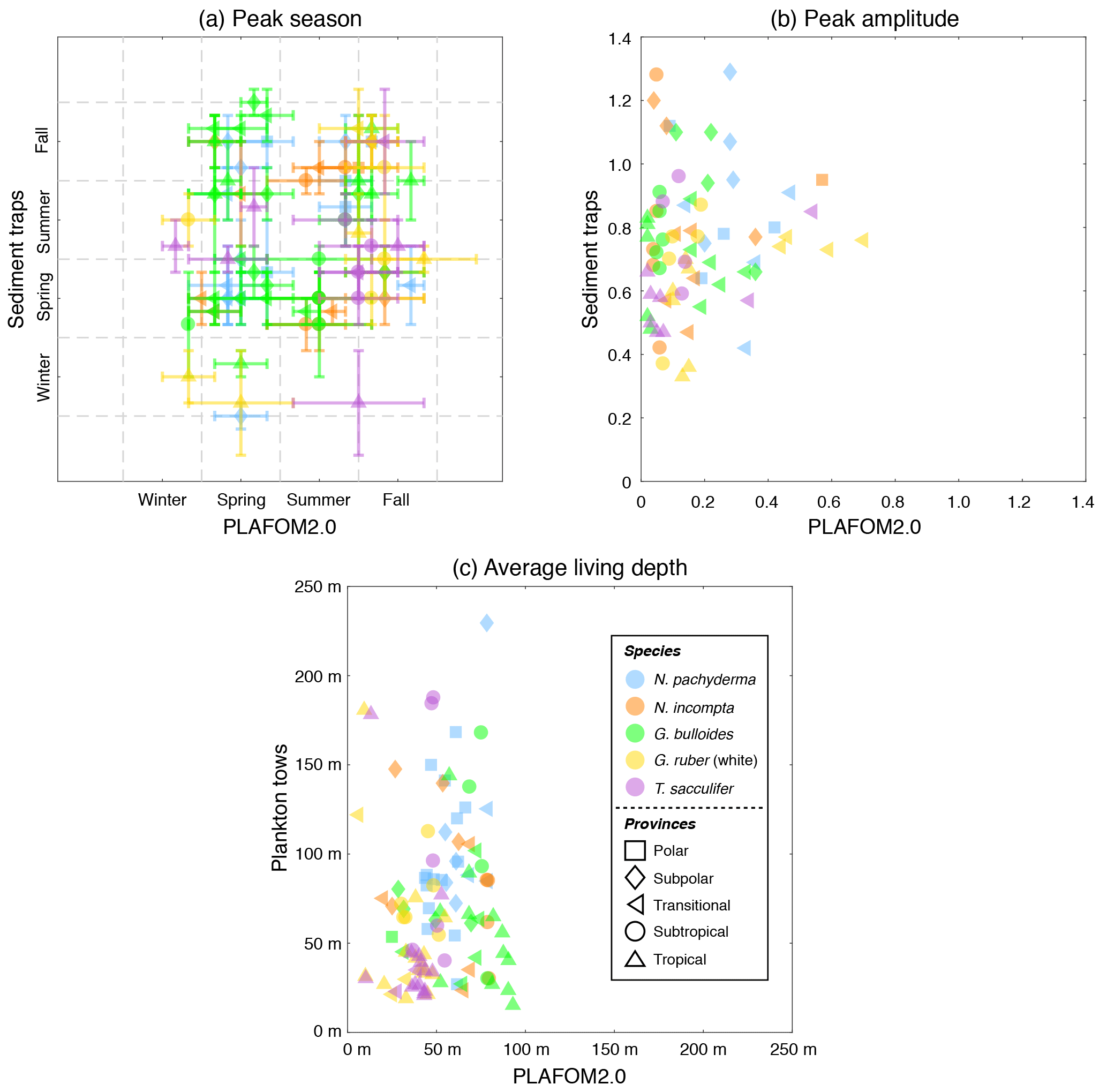
Figure 6(a) Peak seasons (i.e., caloric season of maximum production), (b) peak amplitudes (i.e., maximum production divided by annual mean), and (c) average living depths (in m) for N. pachyderma (light blue), N. incompta (orange), G. bulloides (green), G. ruber (white) (gold), and T. sacculifer (orchid) based on either the sediment trap data (given in Table S3) or the plankton tow data (given in Table S4) vs. PLAFOM2.0. The symbols represent the polar (squares), subpolar (diamonds), transitional (left-pointing triangles), subtropical (circles), and tropical (upward-pointing triangles) provinces of the ocean. The symbols in (a) indicate the month corresponding to the mid-season and the error bars refer to the overall time frame given in Table S3a. Note that the observed and modeled peak amplitudes in (b) have been log transformed.
With these caveats in mind, we compare the results of PLAFOM2.0 with 26 sediment trap records and 45 plankton tow samples from all oceans (Fig. 1b, Tables S1 and S2). Note that the results of the point-by-point comparative analysis for each site and species are given in the Supplement (see Figs. S3 and S4).
The peak season of the temperate and cold-water species (G. bulloides, N. incompta, and N. pachyderma) is shifted from late summer in the higher latitudes towards spring at the more equatorward-directed locations in the subpolar and transitional water masses both in the model and in the sediment trap records (Fig. 6a, Table S3a). The modeled peak amplitudes of those species remain almost constant at rather low values independent of the considered region. In the sediment traps, however, the peak amplitude values are higher and more diverse, and also no clear pattern is evident for the species or for the provinces changing with latitude (Fig. 6b, Table S3b). In line with the plankton tow samples, N. pachyderma, N. incompta, and G. bulloides occur to a large extent below 50 m of water depth from the cold high latitudes to the warmer provinces. However, the modeled ALDs (ranging between 20 and 100 m) are considerably lower than the observed ALDs, which spread over 250 m (Fig. 6c, Table S4). The warm-water species G. ruber (white) and T. sacculifer occur year-round in the subtropical–tropical regions with no distinct preference for a particular season both in the observations and in the model simulation (Fig. 6a, Table S3a). In the transitional waters, however, their peak fluxes are consistently concentrated in fall, leading to higher peak amplitude values at least in the model (Fig. 6b, Table S3b). Throughout the tropics and subtropics, the modeled peak amplitudes remain constant at low values. In the sediment trap records, however, the peak amplitudes are higher (compared with PLAFOM2.0) and vary within both species and within each province (Fig. 6b). In the tropics, G. ruber (white) and T. sacculifer occur primarily close to the surface with ALDs below 50 m both in the model simulation and in the plankton tow records (Fig. 6c, Table S4). In fact, the predicted ALD values (consistently ranging between the surface and 55 m) are lower in comparison with the observations in the transitional and subtropical waters and accordingly do not exhibit a similar value range as the plankton tow records.
In general, the point-by-point comparison between the observations and the model simulation reveals that the peak seasons are well predicted by PLAFOM2.0. The predicted peak amplitudes and average living depths also show realistic trends, but the model tends to underestimate the magnitude of these trends (Fig. 6). Additionally, some sediment trap flux time series of the temperate and cold-water planktonic foraminiferal species show two seasonal peaks a year (see Jonkers and Kučera, 2015, and Figs. S3 and 7a). PLAFOM2.0 is not always able to faithfully reproduce this bimodal pattern (cf. Figs. S3 and 7a). In the following, we try to identify the causes of discrepancies between the observations and predictions by comparing the model output with exemplarily chosen sediment trap records and/or plankton tow samples of three different locations in each case (Fig. 7).
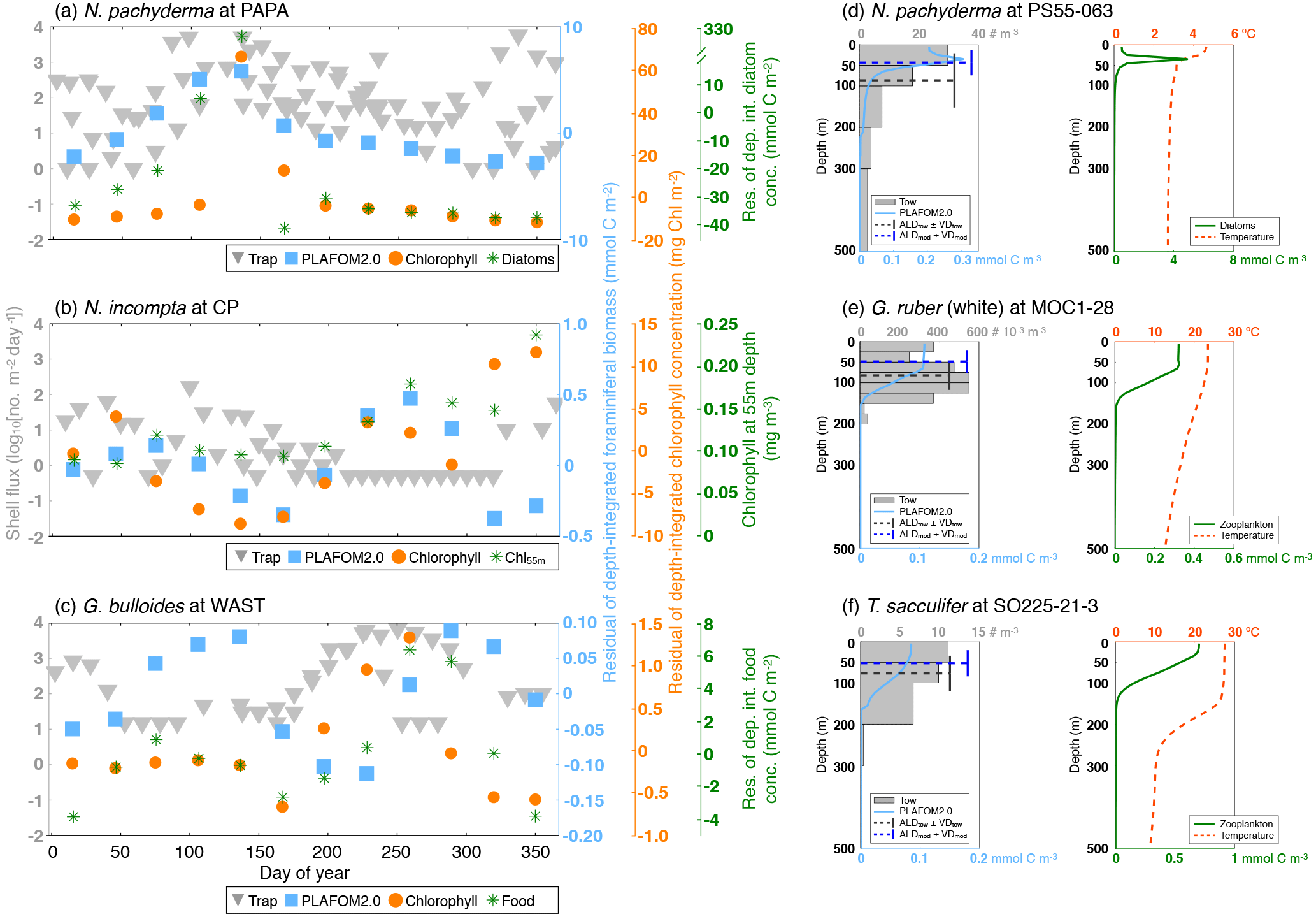
Figure 7(a–c) Comparison of export planktonic foraminiferal shell fluxes in sediment traps (grey triangles) with the residuals (i.e., the deviation from the mean) of the depth-integrated modeled foraminiferal carbon biomass (light blue squares). Note that the difference in the units between sediment trap data (in log10[no. m−2 day−1]) and model output (in mmol C m−2) does not affect the assessment of peak timing. The orange circles denote the residuals of the depth-integrated modeled chlorophyll concentration (in mg Chl m−2), and the dark green asterisks indicate in (a) the residuals of the depth-integrated modeled diatom concentration (in mmol C m−2), in (b) the modeled chlorophyll concentration (in mg m−3) at 55 m of water depth, and/or in (c) the residuals of the sum of the depth-integrated modeled diatom and large detritus (i.e., main food) concentrations (in mmol C m−2). (d–f) Comparison of the vertical distribution of live specimens in plankton tows (in no. m−3; grey bars) with the modeled foraminiferal concentration over depth (in mmol C m−3; light blue profiles). The dashed dark grey and blue lines indicate the average living depth (in m) and vertical dispersion calculated for the plankton tows (ALDtow±VDtow) and PLAFOM2.0 (ALDmod±VDmod), respectively. The dashed red lines denote the predicted temperature profiles (in ∘C), whereas the dark green lines correspond to the modeled vertical distribution of (d) diatoms (in mmol C m−3) and/or (e–f) zooplankton (in mmol C m−3). Data series of (a) N. pachyderma at site PAPA, (b) N. incompta at site CP, and (c) G. bulloides at site WAST. Depth profiles of (d) N. pachyderma at station PS55-063, (e) G. ruber (white) at station MOC1-28, and (f) T. sacculifer at station SO225-21-3. The locations of each sediment trap and plankton tow sample are given in Tables S1 and S2, respectively.
The timing of flux pulse(s) of the temperate and cold-water species has, in general, been linked to the timing of the peak in primary productivity (e.g., Fairbanks and Wiebe, 1980; Donner and Wefer, 1994; Wolfteich, 1994; Kohfeld et al., 1996; Mohiuddin et al., 2002, 2004, 2005; Northcote and Neil, 2005; Asahi and Takahashi, 2007; Storz et al., 2009; Wilke et al., 2009; Jonkers and Kučera, 2015). It is known from studies of the North Atlantic Ocean that phytoplankton seasonality changes with latitude, featuring a single spring bloom in the polar and subpolar Atlantic, a bimodal pattern (one large peak in spring, one smaller peak in fall) in the temperate North Atlantic, a single fall–winter bloom in the subtropical Atlantic, and no prominent seasonal cycle in the tropical Atlantic (e.g., Colebrook, 1979, 1982; Taboada and Anadón, 2014; Friedland et al., 2016). The ecosystem model (providing the food information for PLAFOM2.0), however, does not faithfully reproduce the observed seasonal cycle in primary productivity (cf. Fig. 4 in Moore et al., 2002b). The simulated (depth-integrated) chlorophyll concentration, used as an indicator for productivity, only in part shows two cycles per year (Fig. 7a–c). Nevertheless, the peak timings of the (depth-integrated) foraminifera concentration follow the maxima in primary productivity. For instance, the modeled maximum production peak of N. pachyderma at site PAPA coincides with a peak in the diatom concentration (Fig. 7a), N. incompta reaches its maximum in the simulation more likely at depth at site CP following a DCM (Fig. 7b), and the predicted spring and/or fall peak of G. bulloides at site WAST occurs slightly after the peak in the main food concentration or the maximum in the chlorophyll concentration (Fig. 7c). However, the ecosystem model seems to underestimate the seasonality in primary productivity, which most likely leads to the model–data mismatch in the seasonal pattern of the planktonic foraminifera concentration. Additionally, the variability of planktonic foraminifera carbon biomass produced by PLAFOM2.0 is in general too low compared to the observations. This mismatch can be explained by misrepresentations of the foraminiferal carbon biomass or of the foraminifera response (to the environmental forcing) in the model parameterizations or by an underestimation of the driving factors (especially the main food sources as outlined above). The depth habitat of planktonic foraminifera depends on several environmental and ontogenetic factors (e.g., Fairbanks and Wiebe, 1980; Fairbanks et al., 1982; Schiebel et al., 2001; Simstich et al., 2003; Field, 2004; Salmon et al., 2015; Rebotim et al., 2017). The simulated vertical distribution patterns can also be related to food availability and temperature (Fig. 7d–f). For instance, at station PS55-063, peak abundances of N. pachyderma are reached in the top 50 m in the model corresponding to the highest diatom concentrations (Fig. 7d). At station MOC1-28, the predicted depth profile of G. ruber (white) coincides with the vertical distribution pattern of zooplankton with maximum concentrations occurring over the top 50 m of the water column (Fig. 7e). At station SO225-21-3, the modeled species concentration of T. sacculifer decreases gradually with depth following the zooplankton distribution, but also temperature (Fig. 7f). However, the simulated depth profiles differ from the observations, which is also indicated by the differences in the ALDs. In PLAFOM2.0, the foraminiferal species do not occur below 200 m of water depth (cf. Figs. 4 and 7d–f), most likely being restricted through food availability and the ambient temperatures. Thus, depending on the vertical resolution of the sampling intervals of a plankton tow sample, the predicted ALD is very likely lower by several meters than the observed ALD. In summary, PLAFOM2.0 is able to reproduce the observed species behavior with regard to time and depth on a local scale, but is strongly dependent on the input variables (e.g., temperature and the different food sources) provided by both the ocean and the ecosystem model and is thus limited in its capability to match the observations.
Keeping the caveats regarding the model resolution, model parameterizations, model hierarchy, and analytical constraints on the observations in mind, the model–data mismatch might be reduced by a higher model resolution (in time and space), which would in turn increase the computational costs. A higher taxonomic resolution of the considered species (resulting in an increased number of passive tracers and likewise degrees of freedom) and an explicit parameterization of the ontogeny of each individual planktonic foraminifera, thus considering the changes in the species life cycles with depth (e.g., Bijma et al., 1990a; Bijma, 1991; Bijma and Hemleben, 1994; Bijma et al., 1994; Hemleben and Bijma, 1994; Schiebel et al., 1997), could considerably improve the model. The discrepancies between the model and the observations could additionally be minimized by including better ecological constraints on planktonic foraminifera species and their habitat, e.g., by introducing more phytoplankton and zooplankton functional groups in the ecosystem model to better resolve species food preferences, which would, however, result in increased computational costs. Nevertheless, additional knowledge about the factors controlling the habitat of planktonic foraminifera in time and space based on culturing experiments and field studies is needed for an optimization and better validation of the current model version. In addition, due to the model complexity it is not trivial to determine which model component (i.e., POP2, BEC, or PLAFOM2.0) contributes to what extent to the model–data mismatch. Determining this would require a suite of sensitivity experiments with each model component, which should be considered for future work. The model nonetheless produces seasonal and vertical abundance patterns that are consistent with our current understanding and which emerge from the model without an explicit parameterization of abundance in time and space. PLAFOM2.0 thus represents a major step forward from the previous model version and can be used to assess paleoclimate information in a better way.
A new version of the dynamic planktonic foraminifera model PLAFOM (PLAFOM2.0) has been developed and combined with the CESM1.2(BGC) model configuration to simulate species-specific seasonal and depth habitats for N. pachyderma, N. incompta, G. bulloides, G. ruber (white), and T. sacculifer on a global scale. In comparison with the original approach in which only species concentrations in the surface mixed layer were predicted, PLAFOM2.0 includes a vertical component and thus predicts species distribution patterns in space and time more realistically.
PLAFOM2.0 produces spatially and temporally coherent abundance patterns, which agree well with available observations. The model configuration faithfully reproduces the areal extent of the species. In line with core-top data, the modeled global distribution of each foraminifera changes with latitude. Additionally, PLAFOM2.0 successfully predicts patterns in the timing of the peak fluxes of planktonic foraminiferal species on a global scale. The earlier-when-warmer pattern for the temperate and cold-water species and the flux focusing at low temperatures of warm-water species, as inferred from observations by Jonkers and Kučera (2015), have emerged from the model.
Although an explicit parameterization of the vertical dimension is lacking, the model successfully predicts the preferred habitat depth of the individual planktonic foraminiferal species as well as the spatial and temporal variability in the vertical abundance. In accordance with the available observations, the warm-water species G. ruber (white) and T. sacculifer consistently occur close to the sea surface year-round in the tropics–subtropics, whereas the depth habitat of the colder-water species N. pachyderma, N. incompta, and G. bulloides changes seasonally in the polar–subpolar regions. During the cold season these species occur near the surface, while during the warmer season they descend in the water column to be found up to 120 m of water depth or even below, most likely following the chlorophyll maximum.
In general, paleoceanographic reconstructions based on planktonic foraminifera are hampered by the fact that the environmental signal preserved in their shells is the result of both habitat and climate change. The two effects are difficult to separate without independent data. PLAFOM2.0 presents a powerful tool to address this issue and can contribute to more meaningful comparisons of climate model results and paleoclimate reconstructions, ultimately aiding the understanding of mechanisms of climate change.
All model data can be obtained from the PANGAEA database (https://doi.pangaea.de/10.1594/PANGAEA.892469, Kretschmer et al., 2018). The model code is available upon request from the corresponding author (Kerstin Kretschmer, kkretschmer@marum.de).
The supplement related to this article is available online at: https://doi.org/10.5194/bg-15-4405-2018-supplement.
KK, MK, and MS designed the study. KK developed the model code and designed and finalized the model experiment. KK and LJ analyzed and interpreted the data. All authors contributed to writing the paper.
The authors declare that they have no conflict of interest.
This paper has benefited from the constructive comments and suggestions of
Inge van Dijk, Jelle Bijma, and two anonymous reviewers, as well as of the
handling associated editor Lennart de Nooijer. We are grateful to Graham
Mortyn for providing the plankton tow data from the Atlantic sector of the
Southern Ocean. We would like to thank Gerlinde Jung and Jeroen Groeneveld
for their helpful advice. The model integration has been performed at the
North-German Supercomputing Alliance (HLRN). This project was supported by
the DFG (Deutsche Forschungsgemeinschaft) through the International Research
Training Group IRTG 1904 ArcTrain and the DFG Research Center/Cluster of
Excellence “The Ocean in the Earth System”.
The article processing charges for this open-access
publication were covered by the University of Bremen.
Edited by: Lennart de Nooijer
Reviewed by:
Jelle Bijma, Inge van Dijk,
and two anonymous referees
Anand, P., Elderfield, H., and Conte, M. H.: Calibration of Mg/Ca thermometry in planktonic foraminifera from a sediment trap time series, Paleoceanography, 18, 1050, https://doi.org/10.1029/2002PA000846, 2003. a
Asahi, H. and Takahashi, K.: A 9-year time-series of planktonic foraminifer fluxes and environmental change in the Bering sea and the central subarctic Pacific Ocean, 1990-1999, Prog. Oceanogr., 72, 343–363, https://doi.org/10.1016/j.pocean.2006.03.021, 2007. a, b
Bauch, D., Carstens, J., and Wefer, G.: Oxygen isotope composition of living Neogloboquadrina pachyderma (sin.) in the Arctic Ocean, Earth Planet. Sc. Lett., 146, 47–58, https://doi.org/10.1016/S0012-821X(96)00211-7, 1997. a
Bé, A. W. H.: Some observations on Arctic planktonic foraminifera, Contrib. Cushman Found. Foram. Res., 11, 64–68, 1960. a
Bé, A. W. H.: Planktonic Foraminifera, in: Antarctic Map Folio Series 11: Distribution of Selected Groups of Marine Invertebrates in Waters South of 35∘ S Latitude, 9–12, American Geographical Society, 1969. a, b
Bé, A. W. H. and Hamlin, W. H.: Ecology of Recent Planktonic Foraminifera: Part 3: Distribution in the North Atlantic during the Summer of 1962, Micropaleontology, 13, 87–106, 1967. a
Bé, A. W. H. and Hutson, W. H.: Ecology of Planktonic Foraminifera and Biogeographic Patterns of Life and Fossil Assemblages in the Indian Ocean, Micropaleontology, 23, 369–414, https://doi.org/10.2307/1485406, 1977. a, b, c, d
Bé, A. W. H. and Tolderlund, D. S.: Distribution and ecology of planktonic foraminifera in surface waters of the Atlantic and Indian Oceans, in: The Micropaleontology of Oceans, edited by: Funnell, B. and Riedel, W., 105–150, Cambridge University Press, London, 1971. a, b, c, d, e, f, g
Beckmann, W., Auras, A., and Hemleben, C.: Cyclonic cold-core eddy in the eastern North Atlantic. III. Zooplankton, Marine Ecology – Progress Series, 39, 165–173, https://doi.org/10.3354/meps039165, 1987. a
Bergami, C., Capotondi, L., Langone, L., Giglio, F., and Ravaioli, M.: Distribution of living planktonic foraminifera in the Ross Sea and the Pacific sector of the Southern Ocean (Antarctica), Mar. Micropaleontol., 73, 37–48, https://doi.org/10.1016/j.marmicro.2009.06.007, 2009. a, b, c, d
Bijma, J.: Lunar pulses of carbonate output by spinose planktonic foraminifera, in: Protozoa and Their Role in Marine Processes. NATO ASI Series G: Ecological Sciences, edited by: Reid, P. C., Turley, C. M., and Burkill, P. H., 353–354, Springer, Berlin, Heidelberg, 1991. a
Bijma, J. and Hemleben, C.: Population dynamics of the planktic foraminifer Globigerinoides sacculifer (Brady) from the central Red Sea, Deep-Sea Res. Pt. I, 41, 485–510, 1994. a
Bijma, J., Erez, J., and Hemleben, C.: Lunar and semi-lunar reproductive cycles in some spinose planktonic foraminifers, J. Foramin. Res., 20, 117–127, 1990a. a, b
Bijma, J., Faber Jr., W. W., and Hemleben, C.: Temperature and salinity limits for growth and survival of some planktonic foraminifers in laboratory cultures, J. Foramin. Res., 20, 95–116, 1990b. a, b
Bijma, J., Hemleben, C., and Wellnitz, K.: Lunar-influenced carbonate flux of the planktic foraminifer Globigerinoides sacculifer (Brady) from the central Red Sea, Deep-Sea Res. Pt. I, 41, 511–530, 1994. a
Bird, C., Darling, K. F., Russell, A. D., Davis, C. V., Fehrenbacher, J., Free, A., Wyman, M., and Ngwenya, B. T.: Cyanobacterial endobionts within a major marine planktonic calcifier (Globigerina bulloides, Foraminifera) revealed by 16S rRNA metabarcoding, Biogeosciences, 14, 901–920, https://doi.org/10.5194/bg-14-901-2017, 2017. a
Boltovskoy, E.: Planktonic foraminiferal assemblages of the epipelagic zone and their thanatocoenoses, in: The Micropalaeontology of Oceans, edited by: Funnell, B. M. and Riedel, W. R., 277–288, Cambridge University Press, London, 1971. a
Boltovskoy, E., Boltovskoy, D., Correa, N., and Brandini, F.: Planktic foraminifera from the southwestern Atlantic (30∘–60∘ S): species-specific patterns in the upper 50 m, Mar. Micropaleontol., 28, 53–72, https://doi.org/10.1016/0377-8398(95)00076-3, 1996. a
Bradshaw, J. S.: Ecology of living foraminifera in the North and Equatorial Pacific Ocean, Cushman Foundation for Foraminiferal Research: Contributions, 10, 25–64, 1959. a
Caron, D. A., Bé, A. W. H., and Anderson, O. R.: Effects of variations in light intensity on life processes of the planktonic foraminifer Globigerinoides sacculifer in laboratory culture, Journal of the Marine Biological Association of the United Kingdom, 62, 435–451, https://doi.org/10.1017/S0025315400057374, 1982. a
Caron, D. A., Faber, W. W., and Bé, A. W. H.: Effects of temperature and salinity on the growth and survival of the planktonic foraminifer Globigerinoides sacculifer, Journal of the Marine Biological Association of the United Kingdom, 67, 323–341, https://doi.org/10.1017/S0025315400026643, 1987. a
Carstens, J. and Wefer, G.: Recent distribution of planktonic foraminifera in the Nansen Basin, Arctic Ocean, Deep-Sea Res., 39, S507–S524, 1992. a, b
Colebrook, J. M.: Continuous Plankton Records: Seasonal Cycles of Phytoplankton and Copepods in the North Atlantic Ocean and the North Sea, Mar. Biol., 51, 23–32, https://doi.org/10.1016/0011-7471(66)90628-0, 1979. a
Colebrook, J. M.: Continuous plankton records: seasonal variations in the distribution and abundance of plankton in the North Atlantic Ocean and the North Sea, J. Plankton Res., 4, 435–462, 1982. a
Craig, A. P., Vertenstein, M., and Jacob, R.: A New Flexible Coupler for Earth System Modeling developed for CCSM4 and CESM1, Int. J. High Perform. C., 26, 31–42, https://doi.org/10.1177/1094342011428141, 2012. a
Curry, W. B., Ostermann, D. R., Guptha, M. V. S., and Ittekkot, V.: Foraminiferal production and monsoonal upwelling in the Arabian Sea: evidence from sediment traps, Geological Society, London, Special Publications, 64, 93–106, https://doi.org/10.1144/GSL.SP.1992.064.01.06, 1992. a
Danabasoglu, G., Bates, S. C., Briegleb, B. P., Jayne, S. R., Jochum, M., Large, W. G., Peacock, S., and Yeager, S. G.: The CCSM4 Ocean Component, J. Climate, 25, 1361–1389, https://doi.org/10.1175/JCLI-D-11-00091.1, 2012. a, b, c
Danabasoglu, G., Yeager, S. G., Bailey, D., Behrens, E., Bentsen, M., Bi, D., Biastoch, A., Böning, C., Bozec, A., Canuto, V. M., Cassou, C., Chassignet, E., Coward, A. C., Danilov, S., Diansky, N., Drange, H., Farneti, R., Fernandez, E., Fogli, P. G., Forget, G., Fujii, Y., Griffies, S. M., Gusev, A., Heimbach, P., Howard, A., Jung, T., Kelley, M., Large, W. G., Leboissetier, A., Lu, J., Madec, G., Marsland, S. J., Masina, S., Navarra, A., Nurser, A. J. G., Pirani, A., Salas y Mélia, D., Samuels, B. L., Scheinert, M., Sidorenko, D., Treguier, A.-M., Tsujino, H., Uotila, P., Valcke, S., Voldoire, A., and Wang, Q.: North Atlantic simulations in Coordinated Ocean-ice Reference Experiments phase II (CORE-II). Part I: Mean states, Ocean Model., 73, 76–107, https://doi.org/10.1016/j.ocemod.2013.10.005, 2014. a, b
Darling, K. F., Kucera, M., Pudsey, C. J., and Wade, C. M.: Molecular evidence links cryptic diversification in polar planktonic protists to Quaternary Clim. Dynam., P. Natl. Acad. Sci. USA, 101, 7657–7662, 2004. a
Darling, K. F., Kucera, M., Kroon, D., and Wade, C. M.: A resolution for the coiling direction paradox in Neogloboquadrina pachyderma, Paleoceanography, 21, PA2011, https://doi.org/10.1029/2005PA001189, 2006. a, b, c, d
Darling, K. F., Kucera, M., and Wade, C. M.: Global molecular phylogeography reveals persistent Arctic circumpolar isolation in a marine planktonic protist, P. Natl. Acad. Sci. USA, 104, 5002–5007, https://doi.org/10.1073/pnas.0700520104, 2007. a
Dee, S., Emile-Geay, J., Evans, M. N., Allam, A., Steig, E. J., and Thompson, D. M.: PRYSM: An open-source framework for PRoxY System Modeling, with applications to oxygen-isotope systems, J. Adv. Model. Earth Sy., 7, 1220–1247, https://doi.org/10.1002/2015MS000447, 2015. a
Dee, S. G., Steiger, N. J., Emile-Geay, J., and Hakim, G. J.: On the utility of proxy system models for estimating climate states over the common era, J. Adv. Model. Earth Sy., 8, 1164–1179, https://doi.org/10.1002/2016MS000677, 2016. a
Deuser, W. G., Ross, E. H., Hemleben, C., and Spindler, M.: Seasonal changes in species composition, numbers, mass, size, and isotopic composition of planktonic foraminifera settling into the deep Sargasso Sea, Palaeogeogr. Palaeocl., 33, 103–127, https://doi.org/10.1016/0031-0182(81)90034-1, 1981. a
Doney, S. C., Glover, D. M., and Najjar, R. G.: A new coupled, one-dimensional biological-physical model for the upper ocean: Applications to the JGOFS Bermuda Atlantic Time-series Study (BATS) site, Deep-Sea Res. Pt. II, 43, 591–624, https://doi.org/10.1016/0967-0645(95)00104-2, 1996. a, b
Doney, S. C., Lindsay, K., Fung, I., and John, J.: Natural Variability in a Stable, 1000-Yr Global Coupled Climate-Carbon Cycle Simulation, J. Climate, 19, 3033–3054, https://doi.org/10.1175/JCLI3783.1, 2006. a
Donner, B. and Wefer, G.: Flux and sTable isotope composition of Neogloboquadrina pachyderma and other planktonic foraminifers in the Southern Ocean (Atlantic sector), Deep-Sea Res. Pt. I, 41, 1733–1743, 1994. a, b
Duplessy, J.-C., Blanc, P.-L., and Bé, A. W. H.: Oxygen-18 Enrichment of Planktonic Foraminifera Due to Gametogenic Calcification Below the Euphotic Zone, Science, 213, 1247–1250, 1981. a, b
Eguchi, N. O., Kawahata, H., and Taira, A.: Seasonal Response of Planktonic Foraminifera to Surface Ocean Condition: Sediment Trap Results from the Central North Pacific Ocean, J. Oceanogr., 55, 681–691, 1999. a
Eguchi, N. O., Ujiié, H., Kawahata, H., and Taira, A.: Seasonal variations in planktonic foraminifera at three sediment traps in the Subarctic, Transition and Subtropical zones of the central North Pacific Ocean, Mar. Micropaleontol., 48, 149–163, https://doi.org/10.1016/S0377-8398(03)00020-3, 2003. a
Erez, J.: Calcification Rates, Photosynthesis and Light in Planktonic Foraminifera, in: Biomineralization and Biological Metal Accumulation: Biological and Geological Perspectives Papers presented at the Fourth International Symposium on Biomineralization, Renesse, the Netherlands, 2–5 June 1982, edited by: Westbroek, P. and de Jong, E. W., 307–312, Springer Netherlands, Dordrecht, the Netherlands, https://doi.org/10.1007/978-94-009-7944-4_29, 1983. a
Evans, M. N., Tolwinski-Ward, S. E., Thompson, D. M., and Anchukaitis, K. J.: Applications of proxy system modeling in high resolution paleoclimatology, Quaternary Sci. Rev., 76, 16–28, https://doi.org/10.1016/j.quascirev.2013.05.024, 2013. a
Fairbanks, R. G. and Wiebe, P. H.: Foraminifera and Chlorophyll Maximum: Vertical Distribution, Seasonal Succession, and Paleoceanographic Significance, Science, 209, 1524–1526, 1980. a, b, c, d, e, f
Fairbanks, R. G., Wiebe, P. H., and Bé, A. W. H.: Vertical Distribution and Isotopic Composition of Living Planktonic Foraminifera in the Western North Atlantic, Science, 207, 61–63, 1980. a, b, c, d, e
Fairbanks, R. G., Sverdlove, M., Free, R., Wiebe, P. H., and Bé, A. W. H.: Vertical distribution and isotopic fractionation of living planktonic foraminifera from the Panama Basin, Nature, 298, 841–844, 1982. a, b, c, d, e, f, g
Field, D. B.: Variability in vertical distributions of planktonic foraminifera in the California Current: Relationships to vertical ocean structure, Paleoceanography, 19, PA2014, https://doi.org/10.1029/2003PA000970, 2004. a, b, c, d, e, f, g, h, i, j, k
Fraile, I., Schulz, M., Mulitza, S., and Kucera, M.: Predicting the global distribution of planktonic foraminifera using a dynamic ecosystem model, Biogeosciences, 5, 891–911, https://doi.org/10.5194/bg-5-891-2008, 2008. a, b, c, d, e, f, g, h, i, j, k, l
Fraile, I., Mulitza, S., and Schulz, M.: Modeling planktonic foraminiferal seasonality: Implications for sea-surface temperature reconstructions, Mar. Micropaleontol., 72, 1–9, https://doi.org/10.1016/j.marmicro.2009.01.003, 2009a. a, b
Fraile, I., Schulz, M., Mulitza, S., Merkel, U., Prange, M., and Paul, A.: Modeling the seasonal distribution of planktonic foraminifera during the Last Glacial Maximum, Paleoceanography, 24, PA2216, https://doi.org/10.1029/2008PA001686, 2009b. a, b
Friedland, K. D., Record, N. R., Asch, R. G., Kristiansen, T., Saba, V. S., Drinkwater, K. F., Henson, S., Leaf, R. T., Morse, R. E., Johns, D. G., Large, S. I., Hjøllo, S. S., Nye, J. A., Alexander, M. A., and Ji, R.: Seasonal phytoplankton blooms in the North Atlantic linked to the overwintering strategies of copepods, Elementa: Science of the Anthropocene, 4, 000099, https://doi.org/10.12952/journal.elementa.000099, 2016. a
Ganssen, G. M. and Kroon, D.: The isotopic signature of planktonic foraminifera from NE Atlantic surface sediments: implications for the reconstruction of past oceanic conditions, J. Geol. Soc. London, 157, 693–699, https://doi.org/10.1144/jgs.157.3.693, 2000. a, b
Garcia, H. E., Locarnini, R. A., Boyer, T. P., Antonov, J. I., Zweng, M. M., Baranova, O. K., and Johnson, D. R.: World Ocean Atlas 2009, Volume 4: Nutrients (phosphate, nitrate, silicate), U.S. Government Printing Office, Washington, DC, https://doi.org/10.1182/blood-2011-06-357442, 2010. a
Gastrich, M. D.: Ultrastructure of a new intracellular symbiotic alga found within planktonic foraminifera, J. Phycol., 23, 623–632, https://doi.org/10.1111/j.1529-8817.1987.tb04215.x, 1987. a
Gastrich, M. D. and Bartha, R.: Primary productivity in the planktonic foraminifer Globigerinoides ruber (D'Orbigny), J. Foramin. Res., 18, 137–142, 1988. a
Geider, R. J., Maclntyre, H. L., and Kana, T. M.: A dynamic regulatory model of phytoplanktonic acclimation to light, nutrients, and temperature, Limnol. Oceanography, 43, 679–694, 1998. a
Giraudeau, J.: Planktonic foraminiferal assemblages in surface sediments from the south western African continental margin, Mar. Geol., 110, 47–62, https://doi.org/10.1016/0025-3227(93)90104-4, 1993. a, b
Goosse, H., Crespin, E., de Montety, A., Mann, M. E., Renssen, H., and Timmermann, A.: Reconstructing surface temperature changes over the past 600 years using climate model simulations with data assimilation, J. Geophys. Res., 115, D09108, https://doi.org/10.1029/2009JD012737, 2010. a
Griffies, S. M., Biastoch, A., Böning, C., Bryan, F., Danabasoglu, G., Chassignet, E. P., England, M. H., Gerdes, R., Haak, H., Hallberg, R. W., Hazeleger, W., Jungclaus, J., Large, W. G., Madec, G., Pirani, A., Samuels, B. L., Scheinert, M., Gupta, A. S., Severijns, C. A., Simmons, H. L., Treguier, A. M., Winton, M., Yeager, S., and Yin, J.: Coordinated Ocean-ice Reference Experiments (COREs), Ocean Model., 26, 1–46, https://doi.org/10.1016/j.ocemod.2008.08.007, 2009. a
Hakim, G. J., Emile-Geay, J., Steig, E. J., Noone, D., Anderson, D. M., Tardif, R., Steiger, N., and Perkins, W. A.: The last millennium climate reanalysis project: Framework and first results, J. Geophys. Res.-Atmos., 121, 6745–6764, https://doi.org/10.1002/2016JD024751, 2016. a
Hemleben, C. and Bijma, J.: Foraminiferal Population Dynamics And STable Carbon Isotopes, in: Carbon Cycling in the Glacial Ocean: Constraints on the Ocean's Role in Global Change, edited by: Zahn, R., Pedersen, T. F., Kaminski, M. A., and Labeyrie, L., 145–166, Springer, Berlin, Heidelberg, 1994. a
Hemleben, C., Spindler, M., and Anderson, O. R.: Modern Planktonic Foraminifera, Springer, New York, 1989. a, b
Holland, M. M., Bailey, D. A., Briegleb, B. P., Light, B., and Hunke, E.: Improved Sea Ice Shortwave Radiation Physics in CCSM4: The Impact of Melt Ponds and Aerosols on Arctic Sea Ice, J. Climate, 25, 1413–1430, https://doi.org/10.1175/JCLI-D-11-00078.1, 2012. a
Hunke, E. C. and Lipscomb, W. H.: CICE: The Los Alamos Sea Ice Model, Documentation and Software User's Manual, version 4.0, Tech. rep., Los Alamos National Laboratory, 2008. a
Hurrell, J. W., Holland, M. M., Gent, P. R., Ghan, S., Kay, J. E., Kushner, P. J., Lamarque, J.-F., Large, W. G., Lawrence, D., Lindsay, K., Lipscomb, W. H., Long, M. C., Mahowald, N., Marsh, D. R., Neale, R. B., Rasch, P., Vavrus, S., Vertenstein, M., Bader, D., Collins, W. D., Hack, J. J., Kiehl, J., and Marshall, S.: The Community Earth System Model: A framework for collaborative research, B. Am. Meteorol. Soc., 94, 1339–1360, https://doi.org/10.1175/BAMS-D-12-00121.1, 2013. a, b
Husum, K. and Hald, M.: Arctic planktic foraminiferal assemblages: Implications for subsurface temperature reconstructions, Mar. Micropaleontol., 96–97, 38–47, https://doi.org/10.1016/j.marmicro.2012.07.001, 2012. a
Iwasaki, S., Kimoto, K., Kuroyanagi, A., and Kawahata, H.: Horizontal and vertical distributions of planktic foraminifera in the subarctic Pacific, Mar. Micropaleontol., 130, 1–14, https://doi.org/10.1016/j.marmicro.2016.12.001, 2017. a, b, c, d, e, f
Jodłowska, S. and Śliwińska, S.: Effects of light intensity and temperature on the photosynthetic irradiance response curves and chlorophyll fluorescence in three picocyanobacterial strains of Synechococcus, Photosynthetica, 52, 223–232, https://doi.org/10.1007/s11099-014-0024-y, 2014. a, b
Jonkers, L. and Kucera, M.: Global analysis of seasonality in the shell flux of extant planktonic Foraminifera, Biogeosciences, 12, 2207–2226, https://doi.org/10.5194/bg-12-2207-2015, 2015. a, b, c, d, e, f, g, h, i, j, k, l, m
Jonkers, L. and Kucera, M.: Quantifying the effect of seasonal and vertical habitat tracking on planktonic foraminifera proxies, Clim. Past, 13, 573–586, https://doi.org/10.5194/cp-13-573-2017, 2017. a, b
Jonkers, L., Brummer, G.-J. A., Peeters, F. J. C., van Aken, H. M., and De Jong, M. F.: Seasonal stratification, shell flux, and oxygen isotope dynamics of left-coiling N. pachyderma and T. quinqueloba in the western subpolar North Atlantic, Paleoceanography, 25, PA2204, https://doi.org/10.1029/2009PA001849, 2010. a
Jonkers, L., van Heuven, S., Zahn, R., and Peeters, F. J. C.: Seasonal patterns of shell flux, δ18O and δ13C of small and large N. pachyderma (s) and G. bulloides in the subpolar North Atlantic, Paleoceanography, 28, 164–174, https://doi.org/10.1002/palo.20018, 2013. a, b
Jørgensen, B. B., Erez, J., Revsbech, N. P., and Cohen, Y.: Symbiotic photosynthesis in a planktonic foraminiferan, Globigerinoides sacculifer (Brady), studied with microelectrodes, Limnol. Oceanogr., 30, 1253–1267, https://doi.org/10.4319/lo.1985.30.6.1253, 1985. a, b, c
Kemle-von Mücke, S. and Oberhänsli, H.: The Distribution of Living Planktic Foraminifera in Relation to Southeast Atlantic Oceanography, in: Use of Proxies in Paleoceanography, 91–115, Springer, Berlin, Heidelberg, 1999. a, b
Key, R. M., Kozyr, A., Sabine, C. L., Lee, K., Wanninkhof, R., Bullister, J. L., Feely, R. A., Millero, F. J., Mordy, C., and Peng, T.-H.: A global ocean carbon climatology: Results from Global Data Analysis Project (GLODAP), Global Biogeochem. Cy., 18, GB4031, https://doi.org/10.1029/2004GB002247, 2004. a
Kincaid, E., Thunell, R. C., Le, J., Lange, C. B., Weinheimer, A. L., and Reid, F. M. H.: Planktonic foraminiferal fluxes in the Santa Barbara Basin: response to seasonal and interannual hydrographic changes, Deep-Sea Res. Pt. II, 47, 1157–1176, https://doi.org/10.1016/S0967-0645(99)00140-X, 2000. a, b
Kohfeld, K. E., Fairbanks, R. G., Smith, S. L., and Walsh, I. D.: Neogloboquadrina pachyderma (sinistral coiling) as paleoceanographic tracers in polar oceans: Evidence from Northeast Water Polynya plankton tows, sediment traps, and surface sediments, Paleoceanography, 11, 679–699, 1996. a, b, c, d, e, f, g, h, i
Kretschmer, K., Kucera, M., and Schulz, M.: Modeling the distribution and seasonality of Neogloboquadrina pachyderma in the North Atlantic Ocean during Heinrich Stadial 1, Paleoceanography, 31, 986–1010, https://doi.org/10.1002/2015PA002819, 2016. a, b, c, d, e, f, g, h, i, j
Kretschmer, K., Jonkers, L., Kucera, M., and Schulz, M.: Investigation of the seasonal and vertical habitats of planktonic foraminifera using an ecosystem modeling approach, PANGAEA, https://doi.pangaea.de/10.1594/PANGAEA.892469, 2018.
Krishnamurthy, A., Moore, J. K., Zender, C. S., and Luo, C.: Effects of atmospheric inorganic nitrogen deposition on ocean biogeochemistry, J. Geophys. Res., 112, G02019, https://doi.org/10.1029/2006JG000334, 2007. a
Kucera, M.: Planktonic Foraminifera as Tracers of Past Oceanic Environments, in: Proxies in Late Cenozoic Paleoceanography, edited by Hillaire-Marcel, C. and de Vernal, A., chap. 6, 213–262, Elsevier, Amsterdam, https://doi.org/10.1016/S1572-5480(07)01011-1, 2007. a
Kucera, M. and Darling, K. F.: Cryptic species of planktonic foraminifera: their effect on palaeoceanographic reconstructions, Philos. T. R. Soc. Lond., 360, 695–718, 2002. a
Kucera, M., Weinelt, M., Kiefer, T., Pflaumann, U., Hayes, A., Weinelt, M., Chen, M.-T., Mix, A. C., Barrows, T. T., Cortijo, E., Duprat, J., Juggins, S., and Waelbroeck, C.: Reconstruction of sea-surface temperatures from assemblages of planktonic foraminifera: multi-technique approach based on geographically constrained calibration data sets and its application to glacial Atlantic and Pacific Oceans, Quaternary Sci. Rev., 24, 951–998, https://doi.org/10.1016/j.quascirev.2004.07.014, 2005. a, b
Kuroyanagi, A. and Kawahata, H.: Vertical distribution of living planktonic foraminifera in the seas around Japan, Mar. Micropaleontol., 53, 173–196, https://doi.org/10.1016/j.marmicro.2004.06.001, 2004. a, b, c, d, e, f, g, h, i, j, k, l, m, n
Kuroyanagi, A., Kawahata, H., Nishi, H., and Honda, M. C.: Seasonal changes in planktonic foraminifera in the northwestern North Pacific Ocean: sediment trap experiments from subarctic and subtropical gyres, Deep-Sea Res. Pt. II, 49, 5627–5645, https://doi.org/10.1016/S0967-0645(02)00202-3, 2002. a
Large, W. G. and Yeager, S. G.: Diurnal to Decadal Global Forcing For Ocean and Sea-Ice Models: The Data Sets and Flux Climatologies, Tech. Rep. May, NCAR Technical Note NCAR/TN-460+STR, 2004. a
Large, W. G. and Yeager, S. G.: The global climatology of an interannually varying air–sea flux data set, Clim. Dynam., 33, 341–364, https://doi.org/10.1007/s00382-008-0441-3, 2009. a
Lindsay, K., Bonan, G. B., Doney, S. C., Hoffman, F. M., Lawrence, D. M., Long, M. C., Mahowald, N. M., Moore, J. K., Randerson, J. T., and Thornton, P. E.: Preindustrial-Control and Twentieth-Century Carbon Cycle Experiments with the Earth System Model CESM1(BGC), J. Climate, 27, 8981–9005, https://doi.org/10.1175/JCLI-D-12-00565.1, 2014. a, b, c
Lombard, F., Labeyrie, L., Michel, E., Bopp, L., Cortijo, E., Retailleau, S., Howa, H., and Jorissen, F.: Modelling planktic foraminifer growth and distribution using an ecophysiological multi-species approach, Biogeosciences, 8, 853–873, https://doi.org/10.5194/bg-8-853-2011, 2011. a, b
Luo, C., Mahowald, N. M., and del Corral, J.: Sensitivity study of meteorological parameters on mineral aerosol mobilization, transport, and distribution, J. Geophys. Res., 108, 4447, https://doi.org/10.1029/2003JD003483, 2003. a
Mann, K. H. and Lazier, J. R. N.: Dynamics of Marine Ecosystems: Biological-Physical Interactions in the Oceans, Blackwell Publishing Ltd, 2nd edn., 1996. a
Mix, A. C.: The oxygen-isotope record of glaciation, in: The Geology of North America, chap. 6, 111–135, The Geological Society of America, 1987. a
Mohiuddin, M. M., Nishimura, A., Tanaka, Y., and Shimamoto, A.: Regional and interannual productivity of biogenic components and planktonic foraminiferal fluxes in the northwestern Pacific Basin, Mar. Micropaleontol., 45, 57–82, https://doi.org/10.1016/S0377-8398(01)00045-7, 2002. a, b, c
Mohiuddin, M. M., Nishimura, A., Tanaka, Y., and Shimamoto, A.: Seasonality of biogenic particle and planktonic foraminifera fluxes: Response to hydrographic variability in the Kuroshio Extension, northwestern Pacific Ocean, Deep-Sea Res. Pt. I, 51, 1659–1683, https://doi.org/10.1016/j.dsr.2004.06.002, 2004. a, b, c, d, e
Mohiuddin, M. M., Nishimura, A., and Tanaka, Y.: Seasonal succession, vertical distribution, and dissolution of planktonic foraminifera along the Subarctic Front: Implications for paleoceanographic reconstruction in the northwestern Pacific, Mar. Micropaleontol., 55, 129–156, https://doi.org/10.1016/j.marmicro.2005.02.007, 2005. a, b, c
Moore, J. K. and Braucher, O.: Sedimentary and mineral dust sources of dissolved iron to the world ocean, Biogeosciences, 5, 631–656, https://doi.org/10.5194/bg-5-631-2008, 2008. a
Moore, J. K., Doney, S. C., Glover, D. M., and Fung, I. Y.: Iron cycling and nutrient-limitation patterns in surface waters of the World Ocean, Deep-Sea Res. Pt. II, 49, 463–507, 2002a. a
Moore, J. K., Doney, S. C., Kleypas, J. A., Glover, D. M., and Fung, I. Y.: An intermediate complexity marine ecosystem model for the global domain, Deep-Sea Res. Pt. II, 49, 403–462, 2002b. a, b, c, d, e
Moore, J. K., Doney, S. C., and Lindsay, K.: Upper ocean ecosystem dynamics and iron cycling in a global three-dimensional model, Global Biogeochem. Cy., 18, GB4028, https://doi.org/10.1029/2004GB002220, 2004. a, b, c, d, e, f, g, h
Moore, J. K., Doney, S. C., Lindsay, K., Mahowald, N., and Michaels, A. F.: Nitrogen fixation amplifies the ocean biogeochemical response to decadal timescale variations in mineral dust deposition, Tellus, 58B, 560–572, https://doi.org/10.1111/j.1600-0889.2006.00209.x, 2006. a
Moore, J. K., Lindsay, K., Doney, S. C., Long, M. C., and Misumi, K.: Marine Ecosystem Dynamics and Biogeochemical Cycling in the Community Earth System Model [CESM1(BGC)]: Comparison of the 1990s with the 2090s under the RCP4.5 and RCP8.5 Scenarios, J. Climate, 26, 9291–9312, https://doi.org/10.1175/JCLI-D-12-00566.1, 2013. a, b, c, d, e, f, g
Morard, R., Quillévéré, F., Escarguel, G., de Garidel-Thoron, T., de Vargas, C., and Kucera, M.: Ecological modeling of the temperature dependence of cryptic species of planktonic Foraminifera in the Southern Hemisphere, Palaeogeogr. Palaeocl., 391, 13–33, https://doi.org/10.1016/j.palaeo.2013.05.011, 2013. a, b
Mortyn, P. G. and Charles, C. D.: Planktonic foraminiferal depth habitat and δ18O calibrations: Plankton tow results from the Atlantic sector of the Southern Ocean, Paleoceanography, 18, 1037, https://doi.org/10.1029/2001PA000637, 2003. a, b, c, d, e, f, g
Mulitza, S., Wolff, T., Pätzold, J., Hale, W., and Wefer, G.: Temperature sensitivity of planktic foraminifera and its influence on the oxygen isotope record, Mar. Micropaleontol., 33, 223–240, 1998. a
Naidu, P. D. and Malmgren, B. A.: A high-resolution record of late Quaternary upwelling along the Oman Margin, Arabian Sea based on planktonic foraminifera, Paleoceanography, 11, 129–140, 1996. a, b
Northcote, L. C. and Neil, H. L.: Seasonal variations in foraminiferal flux in the Southern Ocean, Campbell Plateau, New Zealand, Mar. Micropaleontol., 56, 122–137, https://doi.org/10.1016/j.marmicro.2005.05.001, 2005. a, b
Nyland, B. F., Jansen, E., Elderfield, H., and Andersson, C.: Neogloboquadrina pachyderma (dex. and sin.) Mg/Ca and δ18O records from the Norwegian Sea, Geochem. Geophy. Geosy., 7, Q10P17, https://doi.org/10.1029/2005GC001055, 2006. a
Ortiz, J. D., Mix, A. C., and Collier, R. W.: Environmental control of living symbiotic and asymbiotic foraminifera of the California Current, Paleoceanography, 10, 987–1009, 1995. a, b, c, d
Ortiz, J. D., Mix, A. C., Rugh, W., Watkins, J. M., and Collier, R. W.: Deep-dwelling planktonic foraminifera of the northeastern Pacific Ocean reveal environmental control of oxygen and carbon isotopic disequilibria, Geochim. Cosmochim. Ac., 60, 4509–4523, 1996. a
Pados, T. and Spielhagen, R. F.: Species distribution and depth habitat of recent planktic foraminifera in Fram Strait, Arctic Ocean, Polar Res., 33, 22483, https://doi.org/10.3402/polar.v33.22483, 2014. a, b, c, d
Peeters, F. J. C. and Brummer, G.-J. A.: The seasonal and vertical distribution of living planktic foraminifera in the NW Arabian Sea, Geological Society, London, Special Publications, 195, 463–497, https://doi.org/10.1144/GSL.SP.2002.195.01.26, 2002. a, b, c, d, e, f, g, h, i, j, k
Pflaumann, U., Duprat, J., Pujol, C., and Labeyrie, L. D.: SIMMAX: A modern analog technique to deduce Atlantic sea surface temperatures from planktonic foraminifera in deep-sea sediments, Paleoceanography, 11, 15–35, 1996. a, b
Pflaumann, U., Sarnthein, M., Chapman, M., de Abreu, L., Funnell, B., Huels, M., Kiefer, T., Maslin, M., Schulz, H., Swallow, J., van Kreveld, S., Vautravers, M., Vogelsang, E., and Weinelt, M.: Glacial North Atlantic: Sea-surface conditions reconstructed by GLAMAP 2000, Paleoceanography, 18, 1065, https://doi.org/10.1029/2002PA000774, 2003. a, b
Pollard, D. and Schulz, M.: A model for the potential locations of Triassic evaporite basins driven by paleoclimatic GCM simulations, Global Planet. Change, 9, 233–249, 1994. a
Prell, W. L., Martin, A., Cullen, J. L., and Trend, M.: The Brown University Foraminiferal Data Base, IGBP PAGES/World Data Center-A for Paleoclimatology, Data Contribution Series # 1999-027, NOAA/NGDC Paleoclimatology Program, Boulder CO, USA, available at: https://www.ncdc.noaa.gov/paleo/metadata/noaa-ocean-5908.html, 1999. a, b
Rebotim, A., Voelker, A. H. L., Jonkers, L., Waniek, J. J., Meggers, H., Schiebel, R., Fraile, I., Schulz, M., and Kucera, M.: Factors controlling the depth habitat of planktonic foraminifera in the subtropical eastern North Atlantic, Biogeosciences, 14, 827–859, https://doi.org/10.5194/bg-14-827-2017, 2017. a, b, c, d, e, f, g, h, i, j, k, l, m, n, o, p, q
Rippert, N., Nürnberg, D., Raddatz, J., Maier, E., Hathorne, E., Bijma, J., and Tiedemann, R.: Constraining foraminiferal calcification depths in the western Pacific warm pool, Mar. Micropaleontol., 128, 14–27, https://doi.org/10.1016/j.marmicro.2016.08.004, 2016. a, b
Salmon, K. H., Anand, P., Sexton, P. F., and Conte, M.: Upper ocean mixing controls the seasonality of planktonic foraminifer fluxes and associated strength of the carbonate pump in the oligotrophic North Atlantic, Biogeosciences, 12, 223–235, https://doi.org/10.5194/bg-12-223-2015, 2015. a, b, c, d, e
Schiebel, R., Bijma, J., and Hemleben, C.: Population dynamics of the planktic foraminifer Globigerina bulloides from the eastern North Atlantic, Deep-Sea Res. Pt. I, 44, 1701–1713, 1997. a, b
Schiebel, R., Waniek, J., Bork, M., and Hemleben, C.: Planktic foraminiferal production stimulated by chlorophyll redistribution and entrainment of nutrients, Deep-Sea Re. Pt I, 48, 721–740, 2001. a, b, c, d, e
Schiebel, R., Waniek, J., Zeltner, A., and Alves, M.: Impact of the Azores Front on the distribution of planktic foraminifers, shelled gastropods, and coccolithophorids, Deep-Sea Res. Pt. II, 49, 4035–4050, 2002. a
Schmidt, D. N., Renaud, S., Bollmann, J., Schiebel, R., and Thierstein, H. R.: Size distribution of Holocene planktic foraminifer assemblages: biogeography, ecology and adaptation, Mar. Micropaleontol., 50, 319–338, 2004. a, b
Schmidt, G. A.: Forward modeling of carbonate proxy data from planktonic foraminifera using oxygen isotope tracers in a global ocean model, Paleoceanography, 14, 482–497, https://doi.org/10.1029/1999PA900025, 1999. a
Sherman, E., Moore, J. K., Primeau, F., and Tanouye, D.: Temperature influence on phytoplankton community growth rates, Global Biogeochem. Cy., 30, 550–559, https://doi.org/10.1002/2015GB005272, 2016. a, b
Simstich, J., Sarnthein, M., and Erlenkeuser, H.: Paired δ18O signals of Neogloboquadrina pachyderma (s) and Turborotalita quinqueloba show thermal stratification structure in Nordic Seas, Mar. Micropaleontol., 48, 107–125, https://doi.org/10.1016/S0377-8398(02)00165-2, 2003. a, b, c, d
Skinner, L. C. and Elderfield, H.: Constraining ecological and biological bias in planktonic foraminiferal Mg/Ca and δ18Occ: A multispecies approach to proxy calibration testing, Paleoceanography, 20, PA1015, https://doi.org/10.1029/2004PA001058, 2005. a
Smith, R., Jones, P., Briegleb, B., Bryan, F., Danabasoglu, G., Dennis, J., Dukowicz, J., Eden, C., Fox-Kemper, B., Gent, P., Hecht, M., Jayne, S., Jochum, M., Large, W., Lindsay, K., Maltrud, M., Norton, N., Peacock, S., Vertenstein, M., and Yeager, S.: The Parallel Ocean Program (POP) reference manual: Ocean component of the Community Climate System Model (CCSM) and Community Earth System Model (CESM), Tech. rep., Los Alamos National Laboratory, 2010. a
Spezzaferri, S., Kucera, M., Pearson, P. N., Wade, B. S., Rappo, S., Poole, C. R., Morard, R., and Stalder, C.: Fossil and Genetic Evidence for the Polyphyletic Nature of the Planktonic Foraminifera “Globigerinoides”, and Description of the New Genus Trilobatus, PLoS ONE, 10, 1–20, https://doi.org/10.1371/journal.pone.0128108, 2015. a
Stangeew, E.: Distribution and Isotopic Composition of Living Planktonic Foraminifera N. pachyderma (sinistral) and T. quinqueloba in the High Latitude North Atlantic, PhD thesis, Christian-Albrechts-Universität zu Kiel, 2001. a
Steiger, N. J., Hakim, G. J., Steig, E. J., Battisti, D. S., and Roe, G. H.: Assimilation of Time-Averaged Pseudoproxies for Climate Reconstruction, J. Climate, 27, 426–441, https://doi.org/10.1175/JCLI-D-12-00693.1, 2014. a
Storz, D., Schulz, H., Waniek, J. J., Schulz-Bull, D. E., and Kučera, M.: Seasonal and interannual variability of the planktic foraminiferal flux in the vicinity of the Azores Current, Deep-Sea Res. Pt. I, 56, 107–124, https://doi.org/10.1016/j.dsr.2008.08.009, 2009. a, b, c, d
Taboada, F. G. and Anadón, R.: Seasonality of North Atlantic phytoplankton from space: Impact of environmental forcing on a changing phenology (1998–2012), Glob. Change Biol., 20, 698–712, https://doi.org/10.1111/gcb.12352, 2014. a
Thiede, J.: Distribution of foraminifera in surface waters of a coastal upwelling area, Nature, 253, 712–714, https://doi.org/10.1038/253712a0, 1975. a, b
Ting, C. S., Rocap, G., King, J., and Chisholm, S. W.: Cyanobacterial photosynthesis in the oceans: The origins and significance of divergent light-harvesting strategies, Trends Microbiol., 10, 134–142, https://doi.org/10.1016/S0966-842X(02)02319-3, 2002. a
van Raden, U. J., Groeneveld, J., Raitzsch, M., and Kucera, M.: Mg/Ca in the planktonic foraminifera Globorotalia inflata and Globigerinoides bulloides from Western Mediterranean plankton tow and core top samples, Mar. Micropaleontol., 78, 101–112, https://doi.org/10.1016/j.marmicro.2010.11.002, 2011. a
Völpel, R., Paul, A., Krandick, A., Mulitza, S., and Schulz, M.: Stable water isotopes in the MITgcm, Geosci. Model Dev., 10, 3125–3144, https://doi.org/10.5194/gmd-10-3125-2017, 2017. a
Watkins, J. M., Mix, A. C., and Wilson, J.: Living planktic foraminifera: tracers of circulation and productivity regimes in the central equatorial Pacific, Deep-Sea Res. Pt. II, 43, 1257–1282, 1996. a, b, c
Watkins, J. M., Mix, A. C., and Wilson, J.: Living planktic foraminifera in the central tropical Pacific Ocean: Articulating the equatorial 'cold tongue' during La Niña, 1992, Mar. Micropaleontol., 33, 157–174, https://doi.org/10.1016/S0377-8398(97)00036-4, 1998. a, b, c, d, e
Wilke, I., Meggers, H., and Bickert, T.: Depth habitats and seasonal distributions of recent planktic foraminifers in the Canary Islands region (29∘ N) based on oxygen isotopes, Deep-Sea Res. Pt. I, 56, 89–106, https://doi.org/10.1016/j.dsr.2008.08.001, 2009. a, b, c, d, e, f, g, h, i, j, k
Wolfteich, C. M.: Satellite-Derived Sea Surface Temperature, Mesoscale Variability, and Foraminiferal Production in the North Atlantic, M.Sc., Cambridge, MS, 1994. a, b, c, d
Yu, E.-F., Francois, R., Bacon, M. P., Honjo, S., Fleer, A. P., Manganini, S. J., Rutgers van der Loeff, M. M., and Ittekot, V.: Trapping efficiency of bottom-tethered sediment traps estimated from the intercepted fluxes of 230Th and 230Pa, Deep-Sea Res. Pt. I, 48, 865–889, https://doi.org/10.1016/S0967-0637(00)00067-4, 2001. a
Žarić, S., Donner, B., Fischer, G., Mulitza, S., and Wefer, G.: Sensitivity of planktic foraminifera to sea surface temperature and export production as derived from sediment trap data, Mar. Micropaleontol., 55, 75–105, https://doi.org/10.1016/j.marmicro.2005.01.002, 2005. a
Žarić, S., Schulz, M., and Mulitza, S.: Global prediction of planktic foraminiferal fluxes from hydrographic and productivity data, Biogeosciences, 3, 187–207, https://doi.org/10.5194/bg-3-187-2006, 2006. a