the Creative Commons Attribution 3.0 License.
the Creative Commons Attribution 3.0 License.
Causes of simulated long-term changes in phytoplankton biomass in the Baltic proper: a wavelet analysis
Jenny Hieronymus
Kari Eilola
Magnus Hieronymus
H. E. Markus Meier
Sofia Saraiva
Bengt Karlson
The co-variation of key variables with simulated phytoplankton biomass in the Baltic proper has been examined using wavelet analysis and results of a long-term simulation for 1850–2008 with a high-resolution coupled physical–biogeochemical circulation model for the Baltic Sea. By focusing on inter-annual variations, it is possible to track effects acting on decadal timescales such as temperature increase due to climate change as well as changes in nutrient input. The strongest inter-annual coherence indicates that variations in phytoplankton biomass are determined by changes in concentrations of the limiting nutrient. However, after 1950 high nutrient concentrations created a less-nutrient-limited regime, and the coherence was reduced. Furthermore, the inter-annual coherence of mixed-layer nitrate with riverine input of nitrate is much larger than the coherence between mixed-layer phosphate and phosphate loads. This indicates a greater relative importance of the vertical flux of phosphate from the deep layer into the mixed layer. In addition, shifts in nutrient patterns give rise to changes in phytoplankton nutrient limitation. The modelled pattern shifts from purely phosphate limited to a seasonally varying regime. The results further indicate some effect of inter-annual temperature increase on cyanobacteria and flagellates. Changes in mixed-layer depth affect mainly diatoms due to their high sinking velocity, while inter-annual coherence between irradiance and phytoplankton biomass is not found.
- Article
(15489 KB) - Full-text XML
- BibTeX
- EndNote


The Baltic Sea is a semi-enclosed brackish water body separated from the North Sea and Kattegat through the Danish straits. It stretches from about 54 to 66∘ N, and the limited water exchange with the ocean in the south gives rise to a large meridional salinity gradient. The circulation is estuarine with a salty deep-water inflow from the ocean and a fresher surface outflow. The Baltic Sea comprises a number of sub-basins connected by sills further restricting the circulation.
The limited water exchange and the long residence time of water have consequences for the biology and the biogeochemistry. The Baltic Sea is naturally prone to eutrophication, and organic matter degradation leads to low deep-water oxygen concentrations in between deep-water renewal events. In turn, this leads to complex nutrient cycling with different processes acting in oxygenized vs. low-oxygen environments.
The Baltic Sea has experienced extensive anthropogenic pressure over the last century. After 1950, intensive use of agricultural fertilizer greatly enhanced the nutrient loads. This led to an expansion of hypoxic bottoms (Carstensen et al., 2014), in turn affecting the cycling of nutrients through the system. Anoxic sediments have lower phosphorus retention capacity, resulting in increased deep-water phosphate concentrations. Consequently, the flux of phosphate to the surface intensified even though the external loads decreased after 1980 in response to improved sewage treatment. Furthermore, as the anoxic area increased, the area of interface between oxic and anoxic zones where denitrification occurs also increased. This resulted in a loss of nitrogen. Vahtera et al. (2007) described these processes as generating a “vicious circle” where decreased concentrations of dissolved inorganic nitrogen (DIN) together with increased phosphate enhanced the relative importance of nitrogen fixation by cyanobacteria.
The importance of this coupling between oxygen and nutrients has been examined in models. Gustafsson et al. (2012) confirmed, using the model BALTSEM, that internal nutrient recycling has increased due to the reduced phosphate retention capacity, resulting in a self-sustained eutrophication where enhanced sedimentary outflux of nutrients together with increased nitrogen fixation outweighs external load reductions.
Satellite monitoring has made it possible to observe changes in several physical and ecological surface variables during the past 3 decades. Significant changes in seasonality have been observed, such as an earlier start of the phytoplankton growth season and timing of chlorophyll maxima (Kahru et al., 2016).
Shifts in nutrient composition and deep-water properties remain difficult to evaluate using observations. Even though the Baltic Sea has a dense observational record from ships, stations and satellites, the longest nutrient records comprise station data from the early 1970 (HELCOM, 2012). For longer time periods the use of a model is required.
In this paper we construct a thorough analysis of the co-variation of phytoplankton biomass with key variables that have been affected by anthropogenic change over the 20th century. Using the Swedish Coastal and Ocean Biogeochemical model (SCOBI; Almroth-Rosell et al., 2011; Eilola et al., 2009) coupled to the 3-D circulation model RCO (Rossby Centre Ocean model; Meier et al., 2003), we scrutinize the effect of nutrient loads, nutrient concentration, temperature, irradiance and mixed-layer depth on the modelled phytoplankton community.
The gap-free data set provided by the model allows us to decompose the variables in time-frequency space using the wavelet transform. Two variables may than be compared using wavelet coherence (Grinsted et al., 2004; Torrence and Compo, 1998).
We have chosen to use a model run spanning the period 1850 to 2009, with which we capture conditions relatively unaffected by anthropogenic forcing as well as current conditions of eutrophication and climate change. Furthermore, we limit our investigation to the Baltic proper so as to capture relatively homogeneous conditions with regards to the biology.
2.1 Model
We have used a run from the model RCO-SCOBI spanning 1850–2009. RCO is a three-dimensional regional ocean circulation model (Meier et al., 2003). It is a z-coordinate model with a free surface and an open boundary in the northern Kattegat. The version used here has a horizontal resolution of 2 nm with 83 depth levels at 3 m intervals.
The biogeochemical interactions are solved by the biogeochemical model SCOBI (Almroth-Rosell et al., 2011; Eilola et al., 2009). The model contains the nutrients phosphate, nitrate and ammonia as well as the plankton functional types representing diatoms, flagellates and others (referred to as flagellates from here on), and cyanobacteria. Furthermore, the model contains nitrogen and phosphorus in one active homogeneous benthic layer.
The model equations can be found in Eilola et al. (2009). Since we are exploring the effect of different variables on the growth of phytoplankton, we will, for clarity, repeat some of them here.
The phytoplankton biomass is described in terms of chlorophyll and with a constant C : Chl ratio. The model thus does not take into account seasonal changes in C : Chl as was found by Jakobsen and Markager (2016):
The net growth of phytoplankton (PHY) is described by the following expression:
Subscript PHY indicates the plankton functional type (diatoms, flagellates or cyanobacteria), and CPHY is the plankton biomass. ANOX is a logarithmic expression that approaches zero as the oxygen concentration becomes small.
LTLIM expresses the phytoplankton light limitation and NUTLIM describes the nutrient limitation. Nutrient limitation follows Michaelis–Menten kinetics, where constant Redfield ratios are assumed in nutrient uptake. NUTLIM is further described in Sect. 2.1.1 and 2.1.2. GMAX is temperature dependent and describes the maximum phytoplankton growth rate.
Diatoms and flagellates have different half-saturation constants, maximum growth rate, temperature dependence and sinking rate. Flagellates are more sensitive to changes in temperature than diatoms. Furthermore, the sinking rate of diatoms is 5 times larger than that for flagellates.
The difference between cyanobacteria and the other phytoplankton is more pronounced. Cyanobacteria can grow either according to Eq. (1) or using nitrogen fixation. The rate of nitrogen fixation is a function of phosphate concentration, N : P ratio and temperature. Both nitrogen fixation and growth of cyanobacteria is zero if the salinity is above 10. Furthermore, cyanobacteria is the most temperature sensitive of the phytoplankton groups, and no sinking is assumed.
Other processes important for our results involves chemical reactions occurring in the water column or in the sediment. Denitrification occurs both in the water column and the benthic layer and constitutes a sink for nitrate in the case of anoxia. Nitrification transforms ammonium into nitrate as long as oxygen is present. Phosphorus is adsorbed to the sediment, and the benthic release capacity of phosphate is a function of the oxygen concentration. The phosphorus release capacity is also dependent on salinity, whereby higher salinity leads to lower retention of phosphate in the benthic layer.
2.1.1 Nutrient limitation
Estimating nutrient limitation in nature is difficult. Usually this is done either by comparing nutrient ratios to Redfield in, e.g., the surface water or external supply or through nutrient enrichment experiments (Granéli et al., 1990).
The implementation of nutrient limitation most commonly used is that the primary production is directly limited by the nutrient concentration in the ambient water and that the internal nutrient ratios in the phytoplankton are constant, i.e. in accordance with a Redfield–Monod model (Redfield, 1958). However, cell-quota type models (Droop, 1973) are being increasingly implemented, and the use of constant internal nutrient ratios is being questioned more and more (Flynn, 2010; Fransner et al., 2018).
In our model, nutrient limitation is expressed assuming constant Redfield ratios, and phytoplankton growth is limited by either nitrogen or phosphate. The degree of nutrient limitation is described by
where NLIMPHY and PLIMPHY are the nitrogen and phosphate limitation, respectively. NLIMPHY is defined as
where
NO3 and NH4 are the concentrations of nitrate and ammonium, and and are the half-saturation constants for nitrate and ammonium uptake, respectively. The exponent in Eq. (4) accounts for inhibition of nitrate uptake in the presence of ammonium (Dortch, 1990; Parker, 1993).
PLIMPHY is modelled as
The constant is the half-saturation constants for phosphate.
Nutrient limitation, NUTLIM, is thus described by a number between 0 and 1, where 1 is no limitation. Since NUTLIM is calculated as the minimum of NLIM and PLIM, NLIM larger than PLIM will temporally cause P limitation of the phytoplankton growth rate. Hence, a different formulation e.g. of NLIM might change a model's sensitivity to the limiting nutrient. Further experiments on this issue are out of the scope of the present paper and left for future studies.
NUTLIM for our model run has been calculated offline from the monthly means according to Eq. (2).
2.1.2 Effect of physical parameters
Changes in cloud cover affect the incoming solar radiation and thus phytoplankton growth. The effect of light is given by the LTLIM term of Eq. (1), which accounts for photo-inhibition.
The mixed-layer depth has been defined as the depth where a density difference of 0.125 kg m−3 from the surface occurs in accordance with what was previously done by e.g. Eilola et al. (2013). The density was calculated from modelled temperature and salinity using the algorithms from Jackett et al. (2006).
2.2 Study area
The Baltic Sea contains several different sub-basins with different characteristics in salinity and nutrient loads. In this study we focus on the Baltic proper as defined in Fig. 1. In order to reduce heterogeneity, we exclude areas shallower than 20 m and put our focus away from the coasts.
We have chosen to use a basin-averaged approach in order to remove local variability and gain a better understanding of the system. All variables have thus been horizontally averaged over the study area. Furthermore, we have also averaged all variables over the mixed layer and from the mixed layer down to a depth of 150 m.
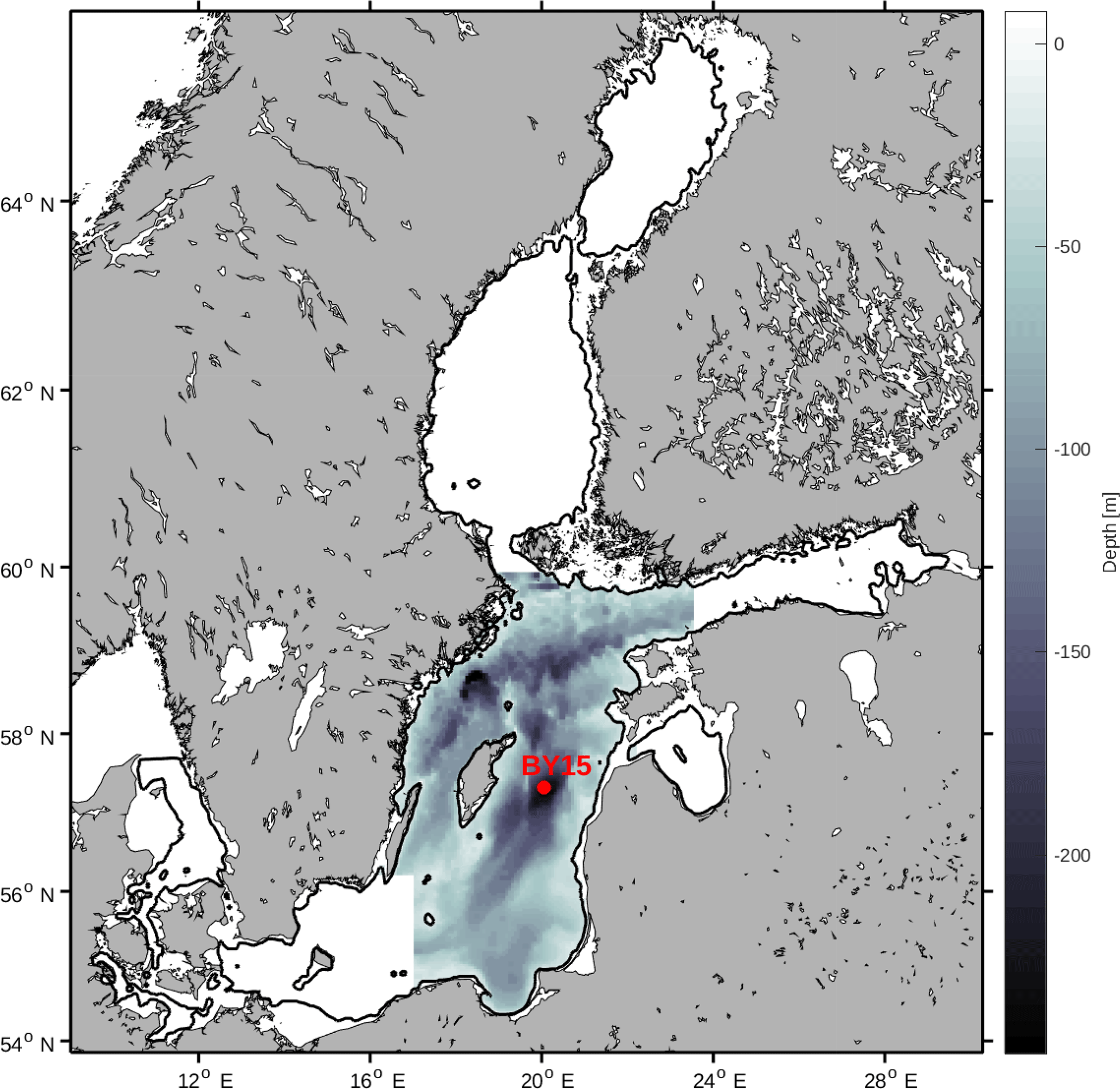
Figure 1Study area. The greyscale represents depth in metres. The red dot represents the monitoring station BY15.
2.3 Forcing
The study uses reconstructed (1850–2008) atmospheric, hydrological and nutrient load forcing, and daily sea levels at the lateral boundary as described by Gustafsson et al. (2012) and Meier et al. (2012). Monthly mean river flows were merged from reconstructions by Hansson et al. (2011) and Meier and Kauker (2003) and hydrological model data from Graham (1999). For further details about the physical model set-up used in the present study the reader is referred to Meier et al. (2017) and references therein.
The nutrient input from rivers and point sources between 1970 and 2006 was compiled from the Baltic Environmental and HELCOM databases (Savchuk et al., 2012). Estimates of pre-industrial loads for 1900 were based on data from Savchuk et al. (2008). The nutrient loads were linearly interpolated between selected reference years in the period between 1900 and 1970. Atmospheric loads were estimated in a similar manner in accordance with Ruoho-Airola et al. (2012). Riverine nutrient loads contain both organic and inorganic phosphorus and nitrogen. Bioavailable fractions of 100 and 30 % were assumed for phosphorus and nitrogen, respectively (Savchuk et al., 2012). No similar distinction between organic and inorganic atmospheric nutrient loads was made (Meier et al., 2018a).
The upper panel of Fig. 2 shows the input of dissolved inorganic phosphorus (DIP) and DIN to the Baltic proper as defined in Fig. 1. The lower panel shows the corresponding simulated mixed-layer concentrations. The loads have been calculated from the runoff and annual mean nutrient concentrations (Eilola et al., 2011). Thus the seasonal cycle in river loads is determined by the runoff. After a spin-up simulation for 1850–1902 utilizing the reconstructed forcing as described above, the calculated physical and biogeochemical variables at the end of the spin-up simulation were used as initial condition for 1850. We have used riverine DIN and DIP loads for our analysis. The use of total bioavailable nutrient loads instead does not change the results.
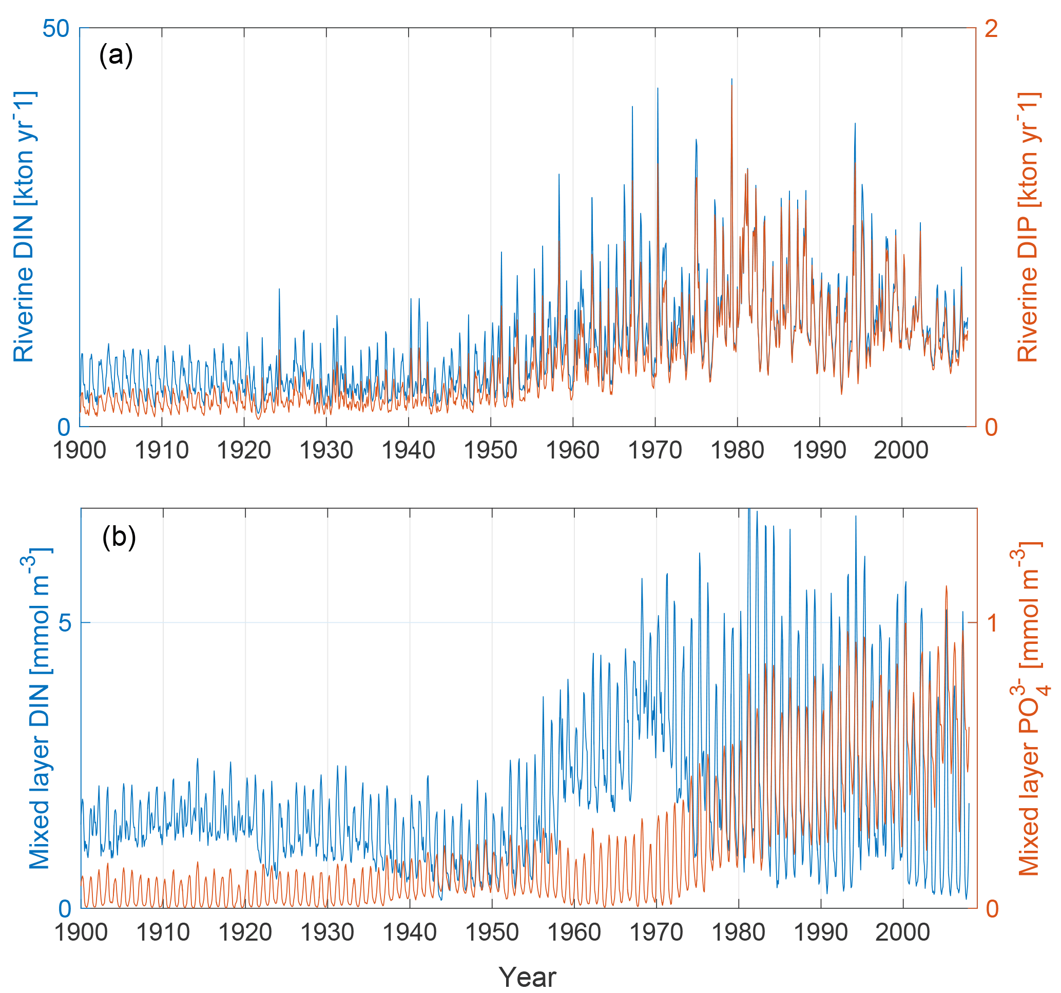
Figure 2Panel (a) shows riverine DIN (blue) and DIP (red) loads to the Baltic proper as defined in Fig. 1. Panel (b) shows mixed-layer DIN (blue) and mixed-layer phosphate (red) averaged over the study area.
The open boundary conditions in the northern Kattegat were based on climatological (1980–2000) seasonal mean nutrient concentrations (Eilola et al., 2009). Similar to Gustafsson et al. (2012) a linear decrease of nutrient concentrations back in time was added, assuming that climatological concentrations in 1900 amounted to 85 % of present-day concentrations (Savchuk et al., 2008). The bioavailable fraction of organic phosphorus at the boundary was assumed to be 100 % in accordance with the organic phosphorus supply from land runoff. Organic nitrogen was implicitly added through the Redfield ratio (nitrogen to phosphorus) of detritus in the model (Eilola et al., 2009).
2.4 Evaluation
The specific model set-up used here has been shown to agree well with observations for salinity, temperature and nutrients (Eilola et al., 2014; Meier et al., 2018a, b). The different phytoplankton functional types have not been previously validated against observations.
The phytoplankton functional groups in the simulations and respective observations from BY15 (see Fig. 1) are shown in Figs. 3 and 4. Phytoplankton biomass from field observations has been estimated through the conversion of biovolumes into carbon in accordance with Menden-Deuer and Lessard (2000). Phytoplankton biomass for the model simulation was estimated from chlorophyll (Chl) assuming a C : Chl ratio of 50. This ratio is in the middle of the salinity-dependent range found by Rakko and Seppälä (2014).
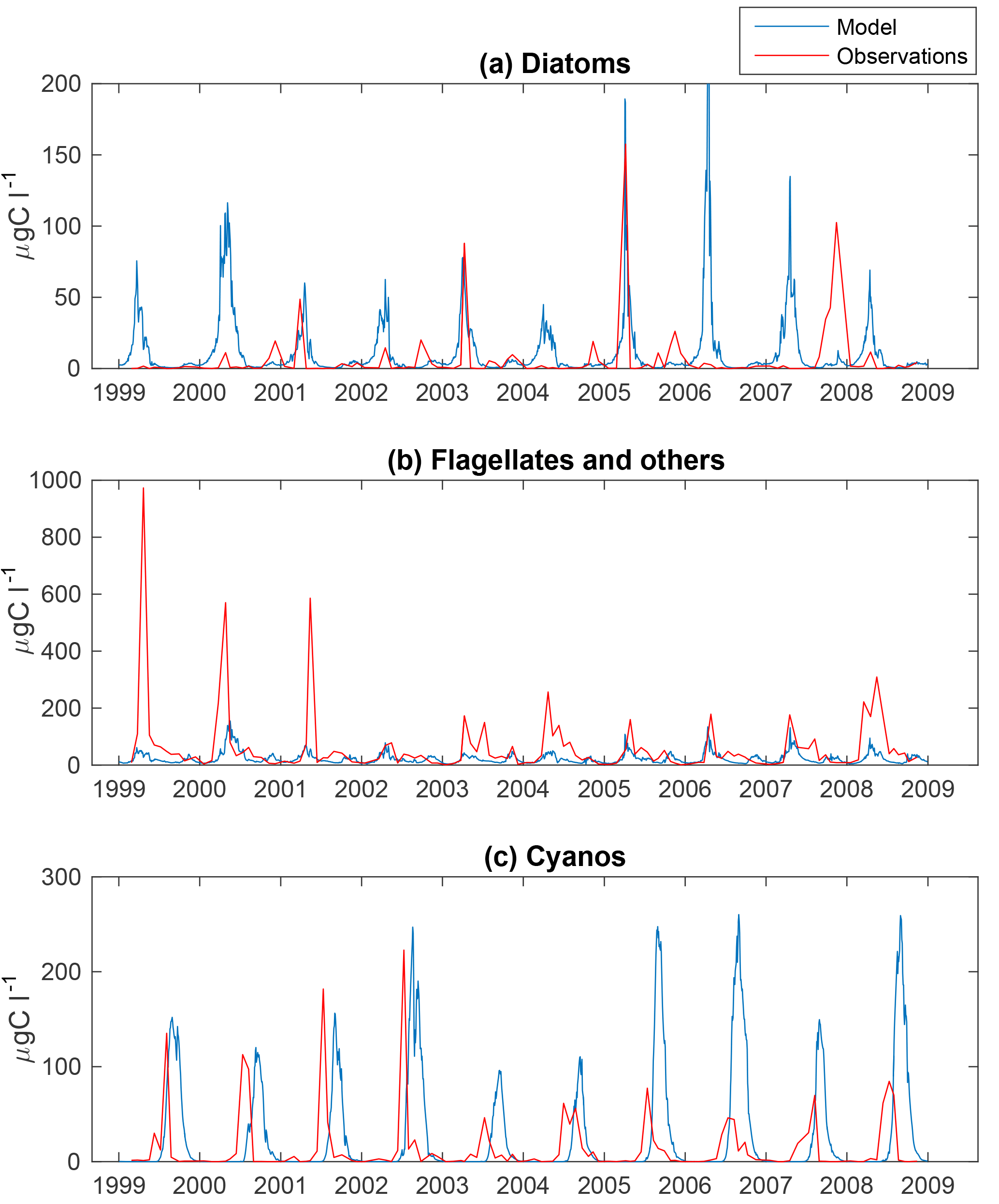
Figure 3Simulated (blue) and observed (red) biomass of diatoms (a), flagellates and others (b) and cyanobacteria (c) at BY15.

Figure 4Monthly means of simulated (a, c, e) and observed (b, d, f) diatoms (a, b), flagellates and others (c, d) and cyanobacteria (e, f) at BY15. Standard deviations are shown as error bars.
The time series display significant inter-annual variability in both model and observations. This variability is also visible as large standard deviations in the modelled and observed monthly means in Figs. 3 and 4.
Figure 4 shows an autumn diatom bloom in the observations, while the model generates an autumn flagellate bloom. In addition, the model partly overestimates the diatom spring blooms. In 2006 and 2007, this is a result of too-high simulated winter nutrient concentrations at BY15. The relationship between modelled N and P also differs from reality, which introduces errors into the distribution of plankton functional types. This may, in part, explain the overestimation of diatoms and the underestimation of flagellates during the first 2 years in Fig. 3.
Similar to comparable models, the simulated cyanobacteria bloom occurs approximately 2 months too late compared to observations (Hense and Beckmann, 2010). It is also notable that the cyanobacteria display strong blooms the first 4 years in both model and observations but that the observations show diminished blooms during the rest of the period where the simulated biomass is still high. There is currently ongoing work of including a cyanobacteria life cycle model, and early work shows some improvements. There is also an influence on the sampling frequency on this comparison. While we have model data every other day, the measurements are only done approximately once a month and will therefore almost certainly miss peak concentration more often than the model values. Differences in the real Chl : C ratio from our fixed value of 50 will also introduce significant errors.
The estimated carbon content from observations is potentially affected by patchiness during in situ sampling and uncertainties related to the calculation of biovolumes and transformation to carbon units.
2.5 The wavelet transform and wavelet coherence
The wavelet transform and its application have been described in several studies (Carey et al., 2016; Grinsted et al., 2004; Lau and Weng, 1995; Torrence and Compo, 1998). Below we provide, therefore, only a brief overview of the method.
The continuous wavelet transform provides a method with which to decompose a signal into time-frequency space. In that it is similar to the windowed Fourier transform where the signal is decomposed within a fixed time-frequency window which is then slid along the time series. However, the fixed width of the window leads to an underestimation of low frequencies. In comparison, the wavelet transform utilizes wavelets with a variable time-frequency window. Wavelets can have many different shapes, and the choice is not arbitrary. We have chosen the commonly used Morlet wavelet, providing good time and frequency localization (Grinsted et al., 2004).
In time-series with clear periodic patterns affected by environmental variables such as population dynamics and ecology the benefits of this approach are significant (Cazelles et al., 2008). In recent years, several studies have highlighted the usefulness of wavelet analyses in plankton research (Carey et al., 2016; Winder and Cloern, 2010). The focus has been the increased availability of long observational data sets making it possible to use the wavelet transform to investigate changes in seasonality. Carey et al. (2016) discussed how the wavelet transform can be used to track inter-annual changes in phytoplankton biomass and applied it to a 16-year time series of phytoplankton in Lake Mendota, USA. In doing so they were able to identify periods when the annual periodicity was less pronounced. They discussed the benefit of this technique in scrutinizing changes to the seasonal succession due to changes in external drivers. Winder and Cloern (2010) applied the technique to time-series of chlorophyll a from marine and freshwater localities and discussed the annual and seasonal periodicities.
Wavelet coherence further expands the usefulness of the wavelet approach by allowing calculation of the time-resolved coherence between two time-series (Cazelles et al., 2008; Grinsted et al., 2004). In this way, it is possible to identify transient periods of correlation over different periodicities. The result is given as coherency as a function of time and period as well as a phase lag between the two time-series.
The disadvantage of wavelet transform analysis is that it requires long data sets without gaps, while on the temporal scale of climate change such observations of plankton dynamics are lacking. Hence, for our purpose only a model-based approach is feasible.
Schimanke and Meier (2016) used wavelet coherency on a multi-centennial model run to evaluate the correlation of different forcing variables with the Baltic Sea salinity. Here we analyse the coherence between modelled phytoplankton biomass and a few key modelled and forcing variables.
For all wavelet calculations we use the Matlab wavelet package described in Grinsted et al. (2004), which is freely available at http://grinsted.github.io/wavelet-coherence/ (last access: 30 July 2018).
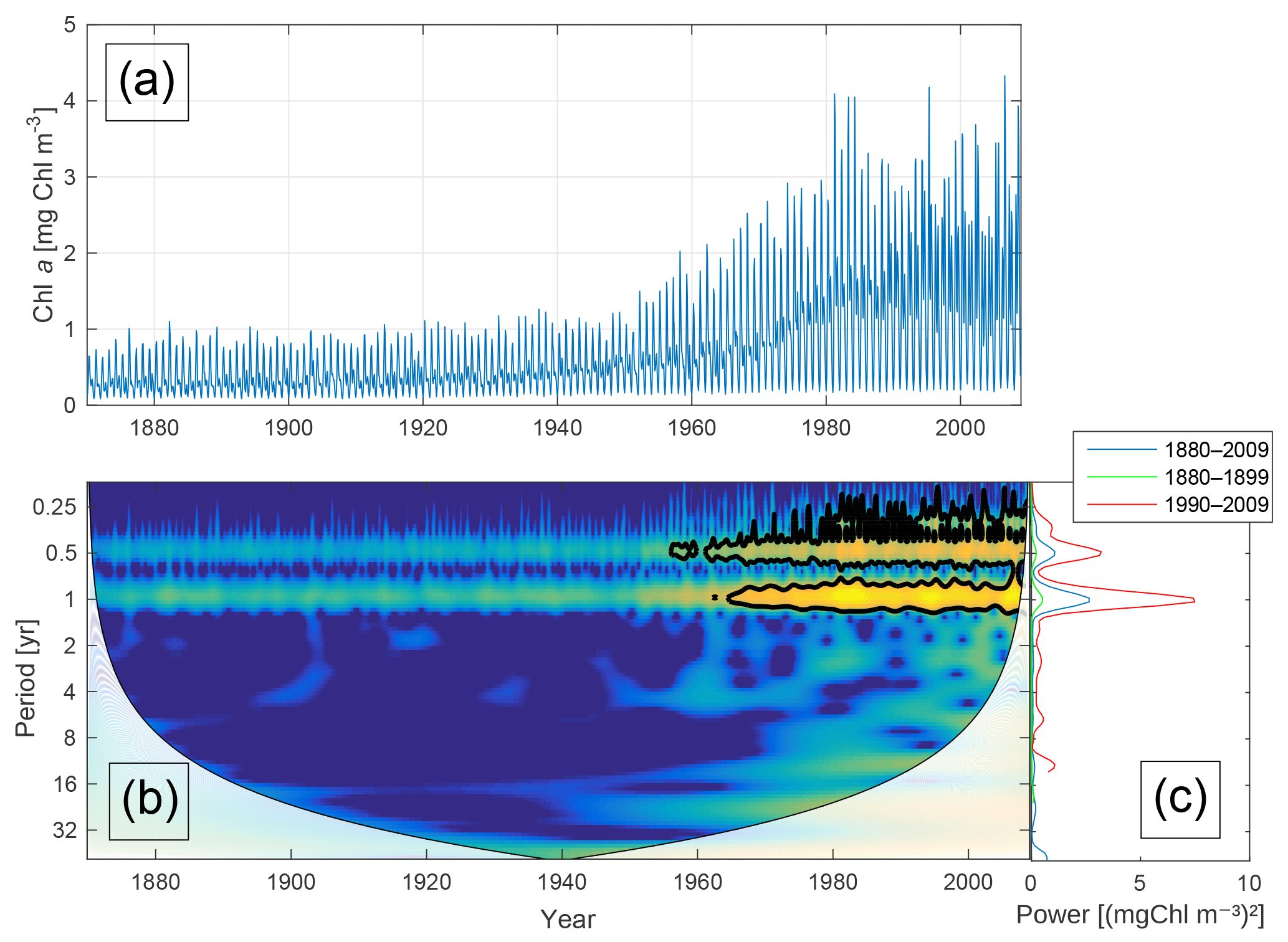
Figure 5Time-series of phytoplankton biomass (a) together with the corresponding wavelet power spectrum (b) and global wavelet spectrum (c). More yellow means more power. The black curves in (b) represent the 95 % confidence level relative to red noise. The white areas in (b) represent the cone of influence in which the results are impacted by edge effects and are therefore not shown. The different lines in (c) represent the global spectrum in 1880–2009 (blue), 1880–1899 (green) and 1990–2009 (red).
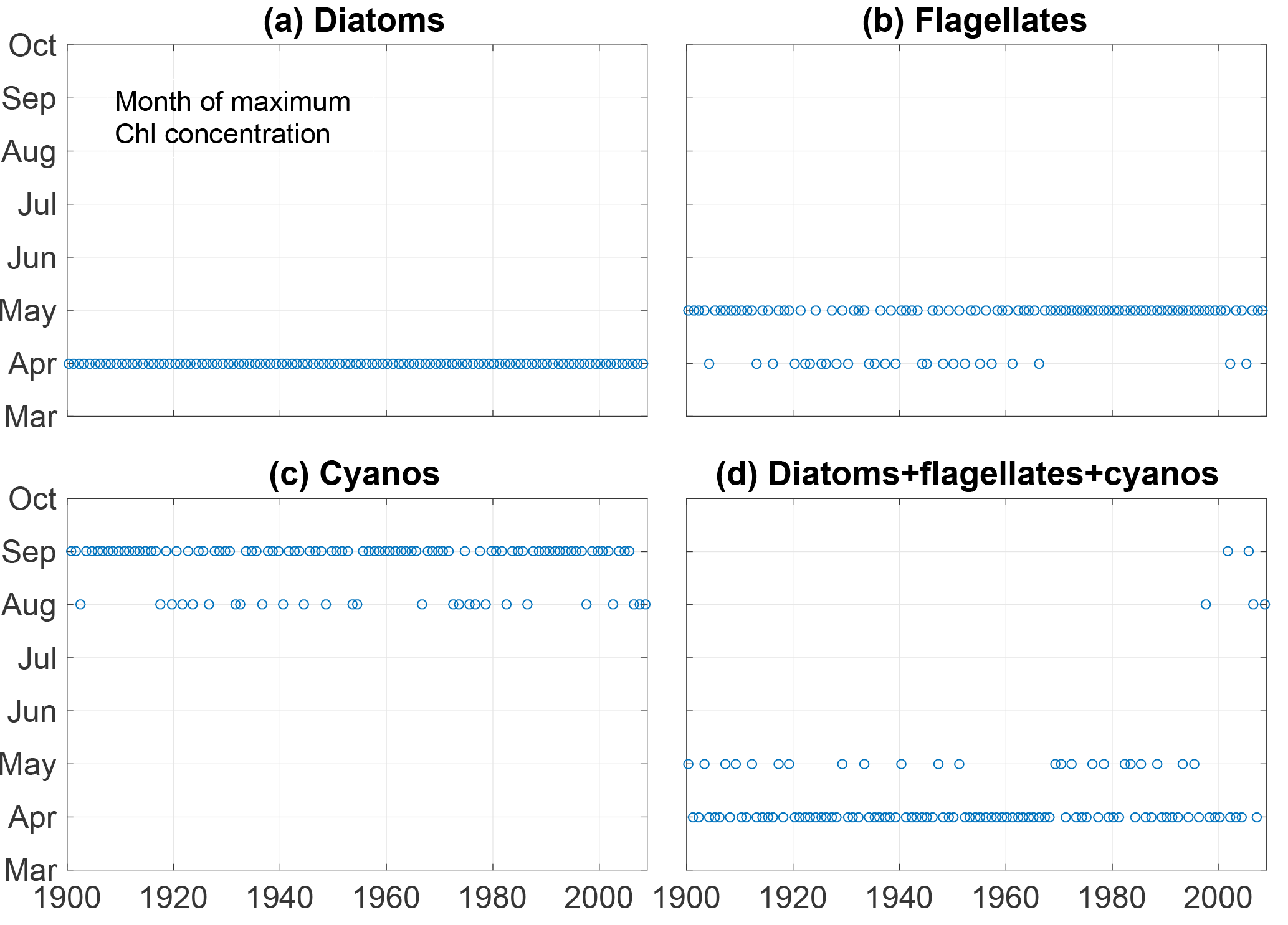
Figure 6The month of maximum biomass of diatoms (a), flagellates (b), cyanobacteria (c) and their sum (d).
We will begin in Sect. 3.1 by presenting the model results on phytoplankton biomass. In Sect. 3.2 we will present the nutrients and their coherence with the phytoplankton biomass. Coherence between riverine loads and mixed-layer nutrients will be discussed in Sect. 3.3. Section 3.4 examines the coherence of phytoplankton with temperature and irradiance. Finally, the coherence between mixed-layer depth and phytoplankton biomass is considered in Sect. 3.5. All results shown are monthly means.
3.1 Phytoplankton biomass
Figure 5 shows the time-series of phytoplankton biomass (panel a) together with the corresponding wavelet spectrum (panel b).
The wavelet power (variance) of the decomposed signal (in colour) is displayed as a function of time (x axis) and period (y axis). The black curves in Fig. 5b show the 95 % confidence level relative to red noise.
Averaging over time generates the global power spectrum displayed in Fig. 5c. The wavelet spectrum clearly reveals two main periodicities – the annual and the semi-annual, representing the spring and autumn blooms. Further, the power of both periodicities increases markedly after 1950.
Kahru et al. (2016) found a shift in chlorophyll maxima from the diatom-dominated spring bloom to the cyanobacteria summer bloom. A similar pattern emerges from our model run as can be seen in Fig. 6. The figure shows the month of maximum biomass of the different phytoplankton species as well as the month of maximum chlorophyll (). After 1998 the results display five years where the month of maximum chlorophyll corresponds to the month of maximum cyanobacteria biomass in August or September.
3.2 Nutrients and nutrient limitation
Increased nutrient loads have caused an increase in primary production and thus also the deep-water respiration, resulting in a 10-fold increase in hypoxic area since the beginning of the 20th century (Carstensen et al., 2014).
This has led to a change in nutrient availability and dynamics as anoxia leads to a release in sedimentary phosphate (e.g. Conley et al., 2002; Savchuk, 2010, 2018; Vahtera et al., 2007). A clear relationship between hypoxia and total basin-averaged phosphate was first shown by Conley et al. (2002) (and later expanded by Savchuk, 2010) on observational data from the Baltic proper.
The effect of hypoxia on DIN is less straightforward. Expanding hypoxia increases the boundary area between anoxic and oxic water where denitrification occurs, resulting in a loss of nitrate. Furthermore, hypoxia causes a reduction in nitrification, leading to a further reduction in nitrate. Vahtera et al. (2007) found a negative relationship between basin-averaged DIN and hypoxic area in observations from the Baltic Sea.
The changing nutrient patterns for our model run are shown in Fig. 7. In conjunction with the increased anoxic volume, we find a clear increase in ammonium and a decrease in nitrate. This is due to a decrease in nitrification and an increase in denitrification. The phosphate concentration increases from the mid-20th century through the rest of the model run as a combined effect of the accumulated terrestrial inputs and hypoxic sedimentary release.
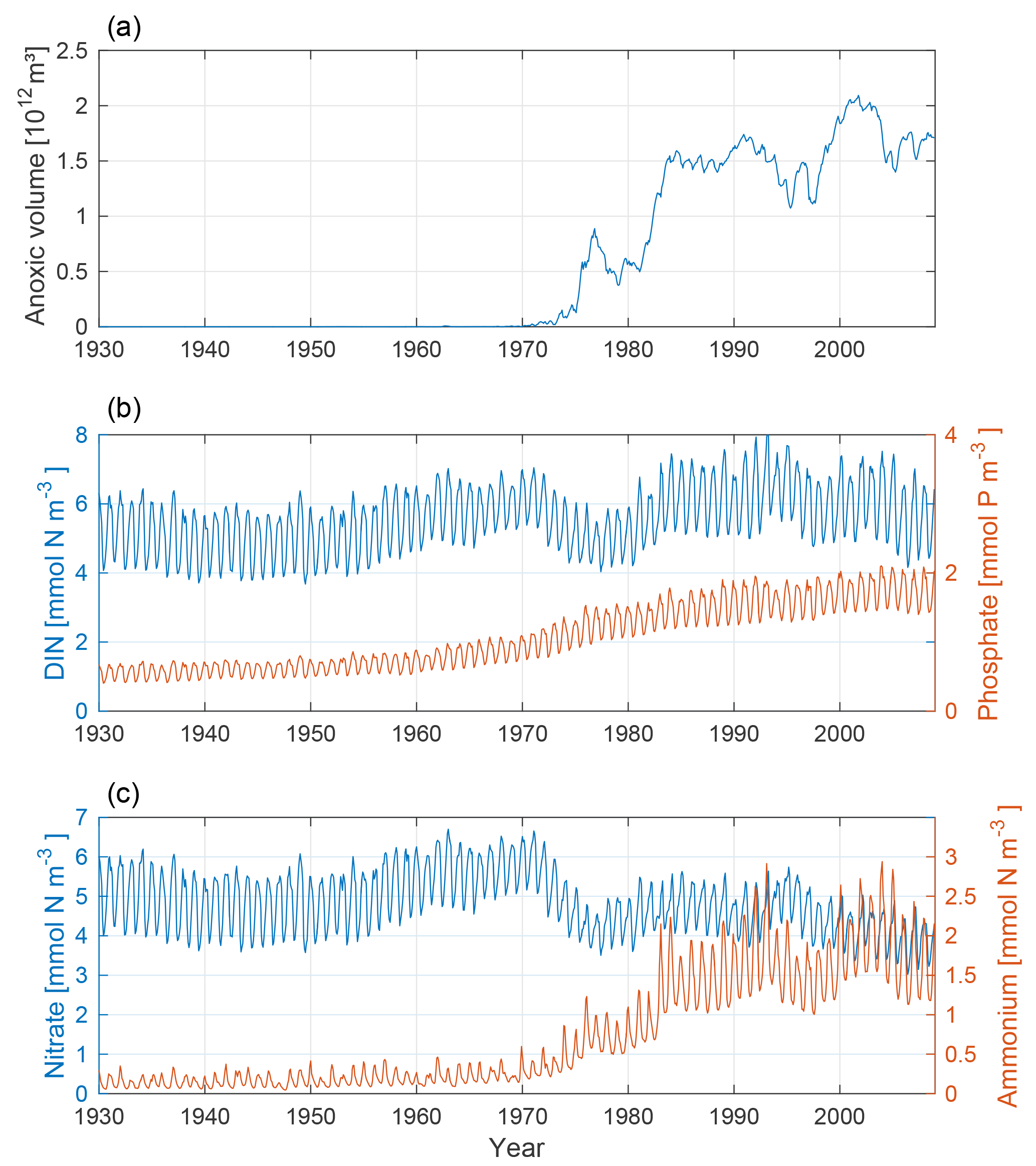
Figure 7Time-series of anoxic volume (a), below-mixed-layer concentrations of DIN (nitrate + ammonium, blue) and phosphate (red) (b), and nitrate (blue) and ammonium (red) (c). Deep-water concentrations were averaged below the mixed-layer depth for the Baltic proper.
The effect of nutrients on the primary production is controlled in the model by the term NUTLIM, or degree of nutrient limitation, in Eq. (1). NUTLIM can be viewed as a measure of the nutrient composition that linearly affects the phytoplankton growth in the model. We examine this term in as well as below the mixed layer as changes in the concentration of nutrients in the deep water will also affect nutrient concentrations in the mixed layer.
The evolutions of NUTLIM in the mixed layer and deep water for diatoms and flagellates are shown in Fig. 8. Mixed-layer values of NUTLIM increase over the 20th century, indicating less-nutrient-limiting conditions.

Figure 8Time-series of nutrient limitation in the mixed layer (a) and below (b) for diatoms (blue) and flagellates (red). The thicker lines in the top panel show the 5-year moving average.
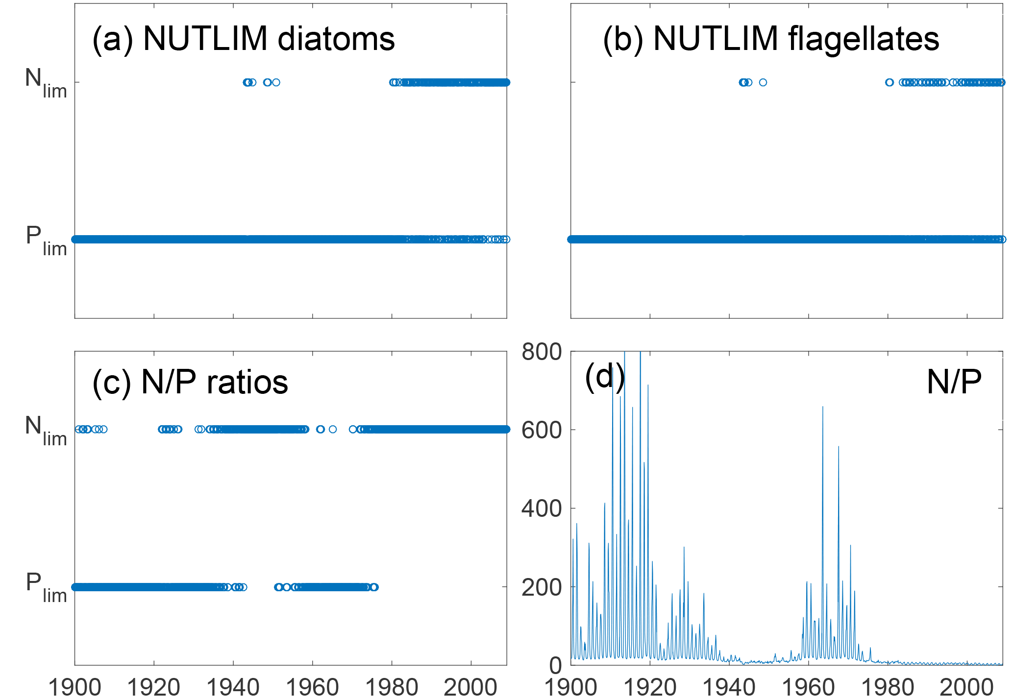
Figure 9Mixed-layer nitrogen or phosphate limitation as a function of time for diatoms (a) and flagellates (b) as calculated through Eq. (2), where N limitation occurs when NLIM < PLIM. Panels (c) and (d) show nutrient limitation as calculated through N ∕ P ratios where N limitation occurs when N ∕ P<16 (c) and actual DIN ∕ phosphate (d). Note that simultaneous N and P limitation is not possible although the size of the rings gives this appearance.
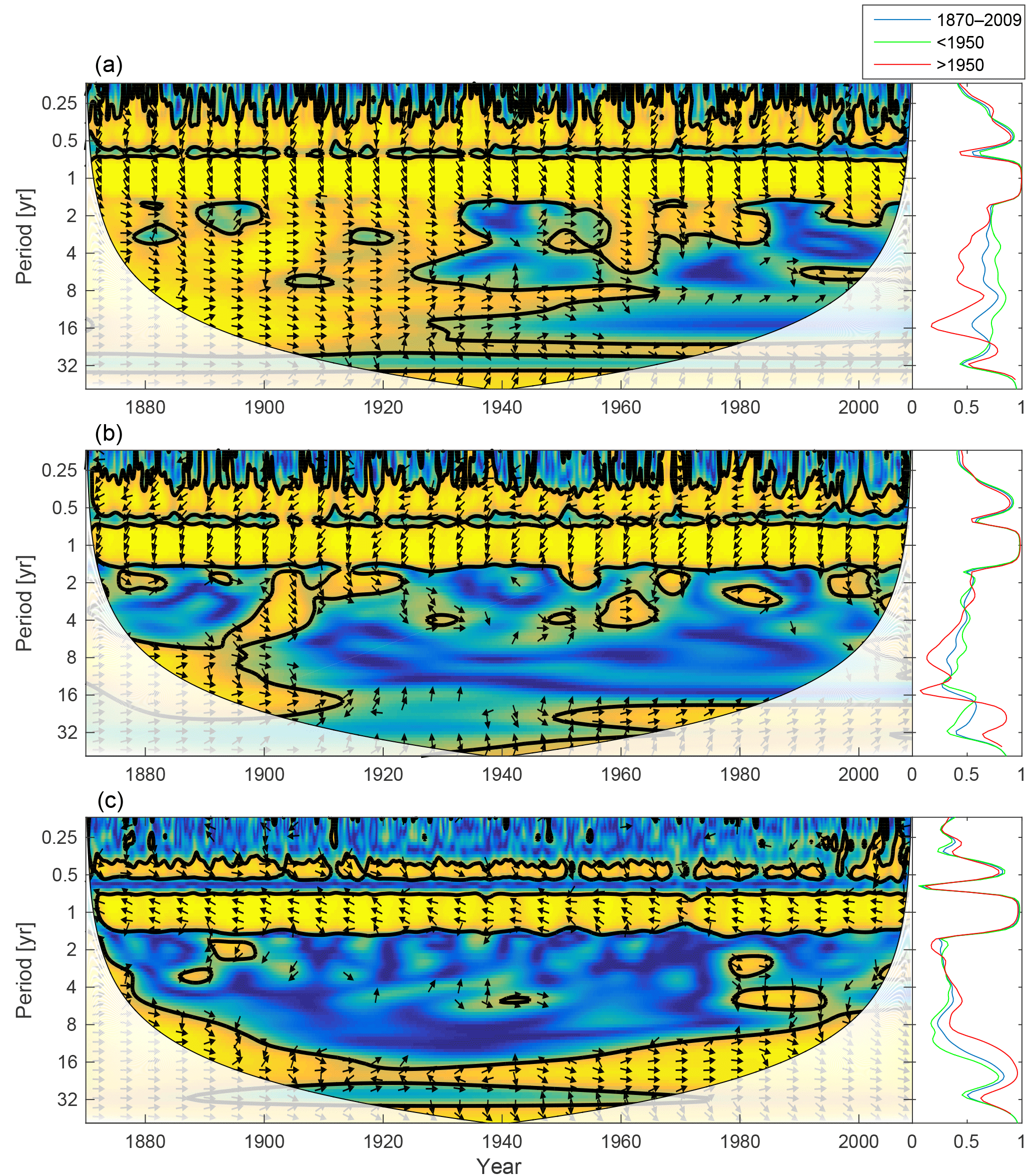
Figure 10Wavelet coherence between mixed-layer phosphate concentration and diatoms (a), flagellates (b) and cyanobacteria (c). More yellow means more coherence. The arrows indicate the phase lag. When pointing to the right, the two time-series are in phase; when pointing in the opposite direction, they are anti-phase. Arrows pointing downwards indicate phosphate preceding plankton group by 90∘, while arrows pointing upwards mean plankton preceding phosphate by the same amount. The right panels show the coherence averaged over the whole period (blue) and before (green) and after (red) 1950.
Nitrogen has been shown to most often limit the growth in the Baltic proper, while phosphate is limiting in the northern basins (Granéli et al., 1990; Tamminen and Andersen, 2007). In pre-industrial conditions, N ∕ P ratios indicate a lesser degree of nitrogen limitation and a higher degree of phosphate limitation for the central Baltic Sea (Gustafsson et al., 2012; Savchuk et al., 2008; Schernewski and Neumann, 2004).
The mixed-layer limitation patterns as estimated from NUTLIM and N ∕ P ratios are shown in Fig. 9. Until 1980, the N ∕ P ratios display a pattern of limitation shifting between nitrogen and phosphate, after which persistent N limitation develops. This weaker N limitation during the first part of the run is consistent with the studies of pre-industrial conditions (Gustafsson et al., 2012; Savchuk et al., 2008; Schernewski and Neumann, 2004).
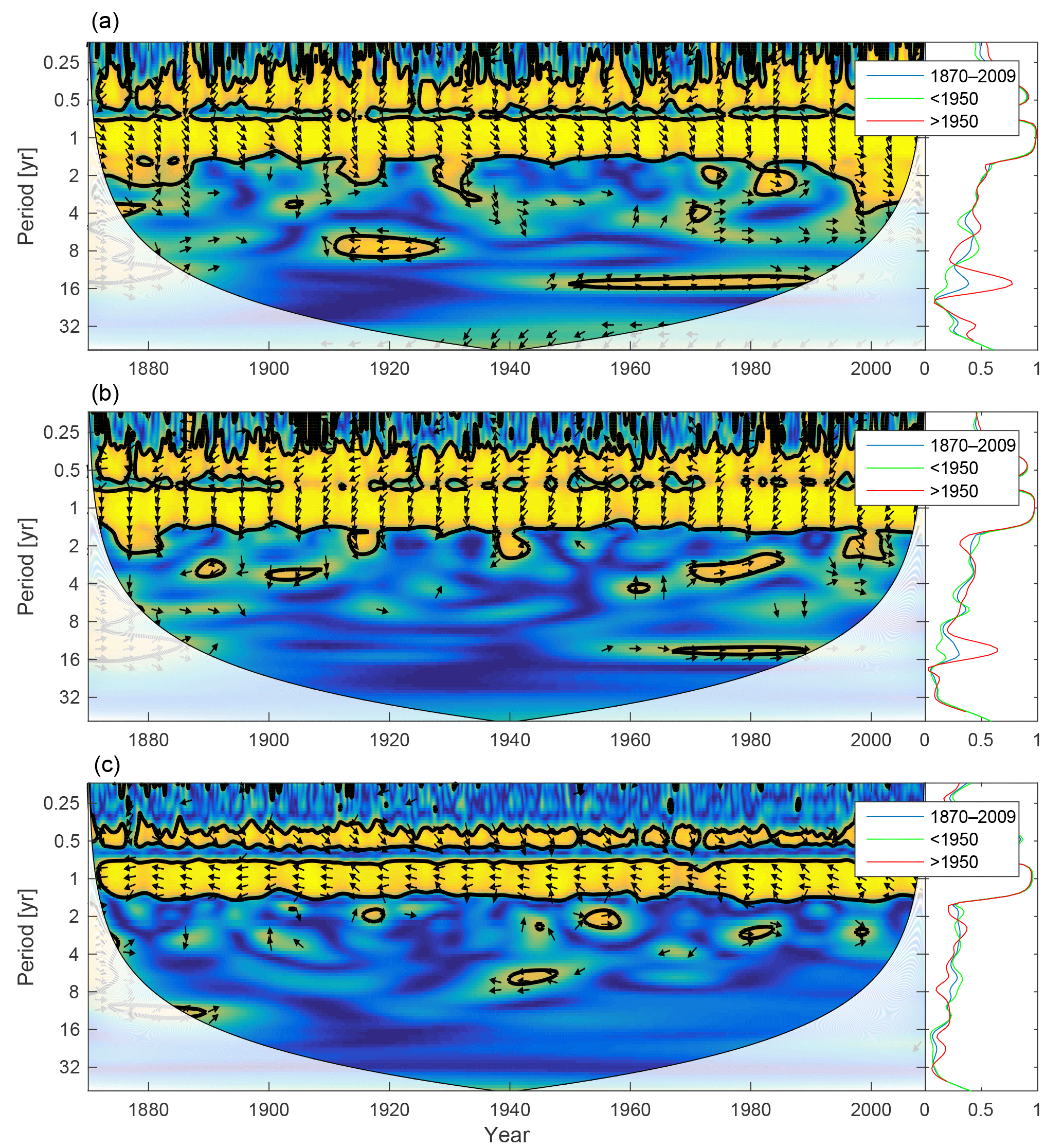
Figure 11Wavelet coherence between mixed-layer DIN concentration and diatoms (a), flagellates (b) and cyanobacteria (c). Arrows pointing downwards indicate DIN preceding plankton group by 90∘, while arrows pointing upwards mean plankton preceding DIN by the same amount. The right panels show the coherence averaged over the whole period (blue) and before (green) and after (red) 1950.
Using NUTLIM, the results instead show phosphate limitation for both diatoms and flagellates for the earlier part of the run. After 1980, a different seasonal pattern appears, with phosphate still limiting during winter, while nitrogen becomes limiting after the spring bloom. Even though the limitation pattern as calculated with NUTLIM differs from what was found using N ∕ P ratios, the overall pattern of increasing degree of N limitation is evident in NUTLIM as well.
The changing nutrient limitation patterns affect phytoplankton growth. We analyse the wavelet coherencies of phytoplankton biomass with mixed-layer phosphate and DIN (the sum of nitrate and ammonium) in Figs. 10 and 11.
As the most strongly nutrient-limited group, diatoms show persistent inter-annual coherence with phosphate during the first, consistently phosphate-limited, part of the run (Fig. 10; see also Fig. 9).

Figure 12Wavelet coherence between deep-water NUTLIM and diatoms (a) and flagellates (b). More yellow means more coherence. Arrows pointing downwards indicate NUTLIM preceding plankton group by 90∘, while arrows pointing upwards mean plankton preceding NUTLIM by the same amount. The right panels show the coherence averaged over the whole period (blue) and before (green) and after (red) 1950.
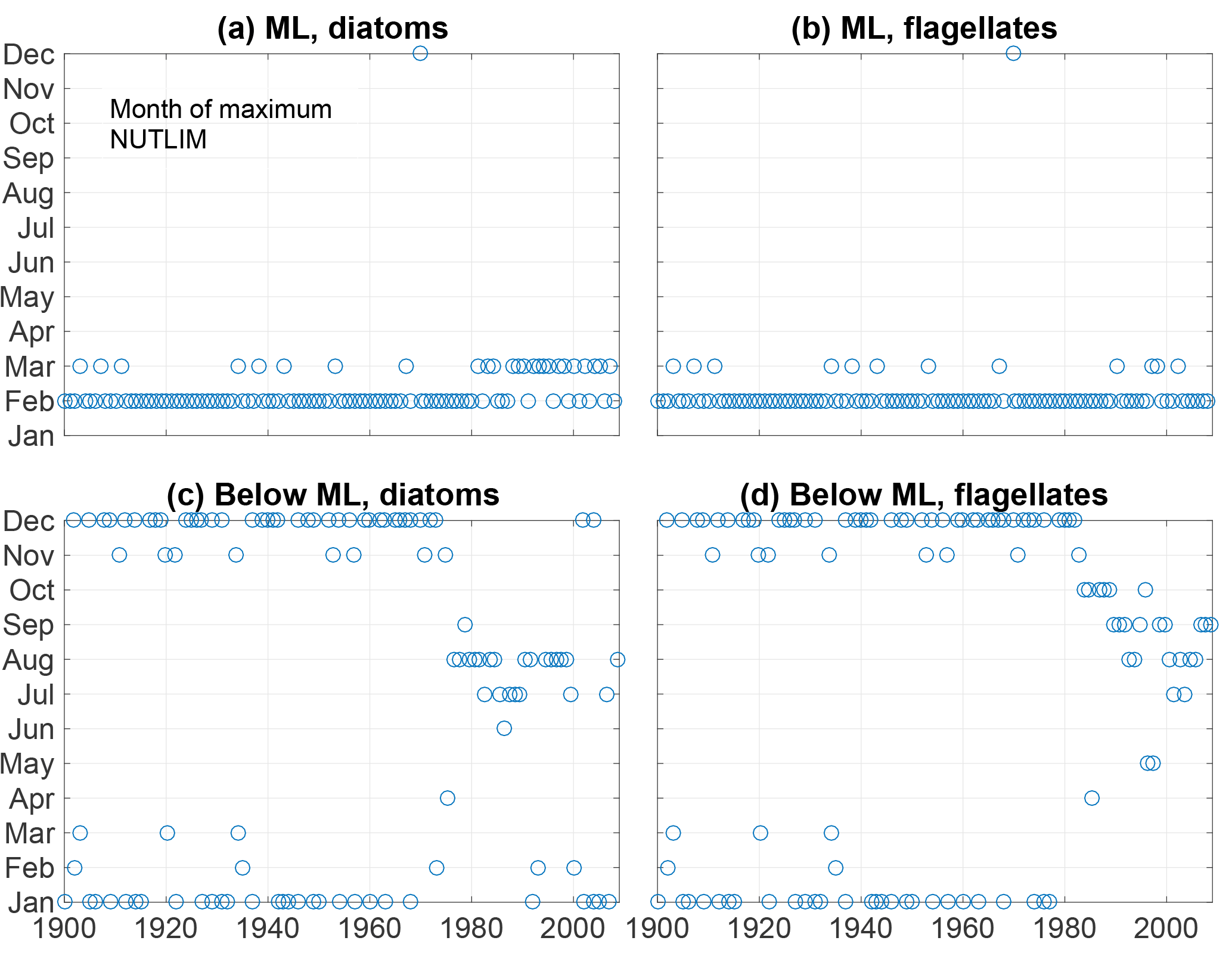
Figure 13The month of maximum NUTLIM for diatoms (a, c) and flagellates (b, d) in the mixed layer (a, b) and below (c, d).
Since nitrogen limitation as calculated with NUTLIM mostly occurs after 1980 and after the spring bloom (Fig. 9), and thus only affects the much smaller diatom and flagellate autumn blooms, little coherence between phytoplankton and nitrogen can be observed on inter-annual timescales (Fig. 11).
To scrutinize the shift in deep-water nutrient composition and the coherence with phytoplankton, we calculate the wavelet coherence between below-mixed-layer NUTLIM and the diatom and flagellate biomass. The result is shown in Fig. 12. After 1980 the phase arrows within the annual coherence period change direction. For diatoms, the phase shifts from NUTLIM preceding diatoms by 3 months to diatoms preceding NUTLIM by the same amount. Flagellates display a similar shift.
The month of maximum NUTLIM shown in Fig. 13 indicates the month when the nutrient composition is most beneficial for phytoplankton growth. The figure shows a clear shift occurring after 1980. Below the mixed layer, NUTLIM changes its maxima from December and January to July, August and September for both diatoms and flagellates, while a slight shift from February to March occurs in mixed-layer NUTLIM for diatoms. Mixed-layer NUTLIM for flagellates displays no clear shift. The shift in NUTLIM is a result of the increase in phosphate and ammonium occurring in conjunction with the increase in anoxic volume shown in Fig. 7. The change in timing is probably due to reduced sedimentary phosphate retention and reduced nitrification after the spring bloom.
3.3 Nutrient loads
We here analyse how changes in nutrient loads affect changes in the mixed-layer nutrient concentrations.
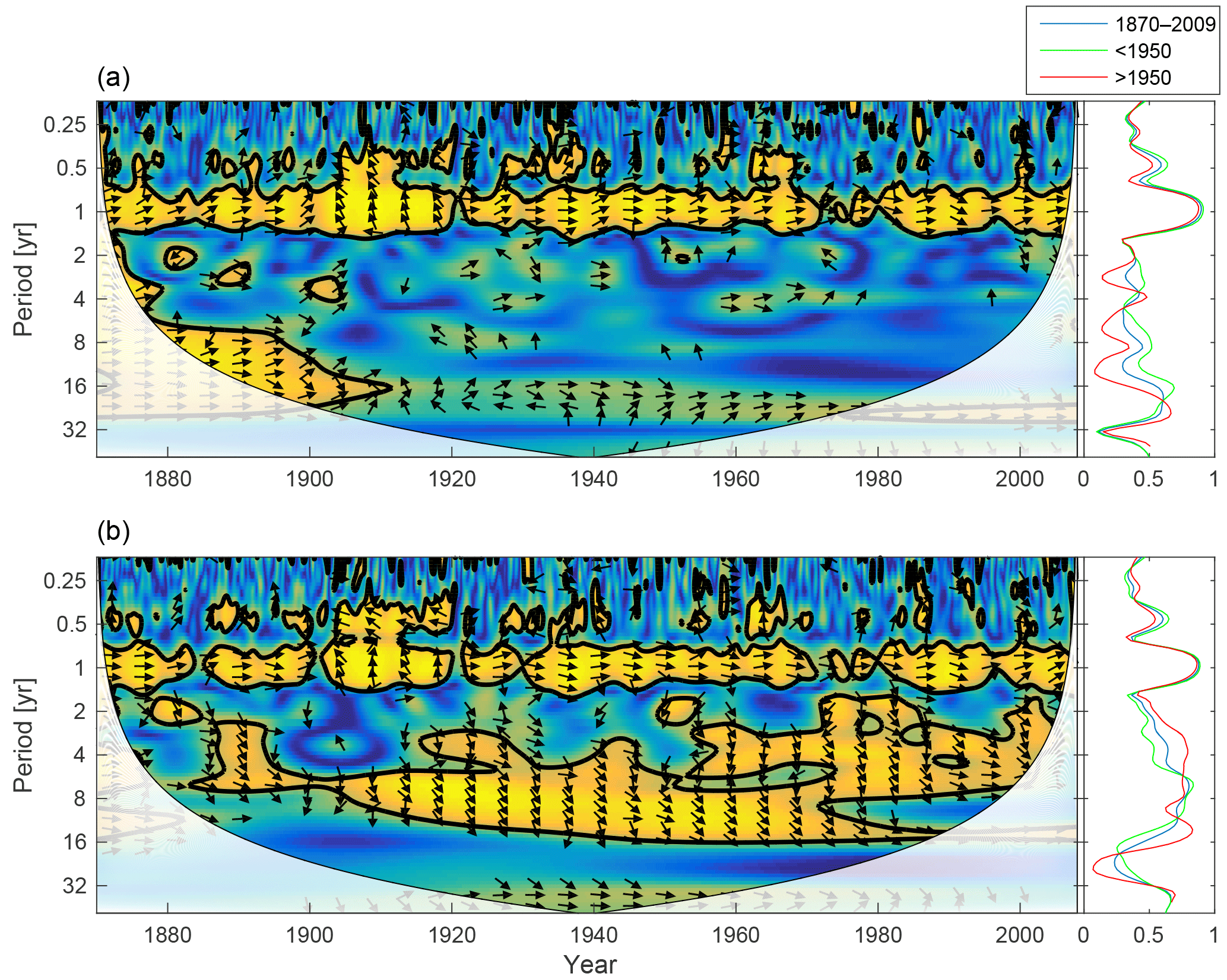
Figure 14Wavelet coherence between riverine phosphate and mixed-layer phosphate concentration (a) and riverine DIN and mixed-layer DIN concentration (b). Arrows pointing downwards indicate riverine phosphate ∕ DIN preceding mixed-layer phosphate ∕ DIN by 90∘, while arrows pointing upwards mean mixed-layer phosphate ∕ DIN preceding riverine phosphate ∕ DIN by the same amount. The right panels show the averaged coherence for the whole period (blue) and before (green) and after (red) 1950.
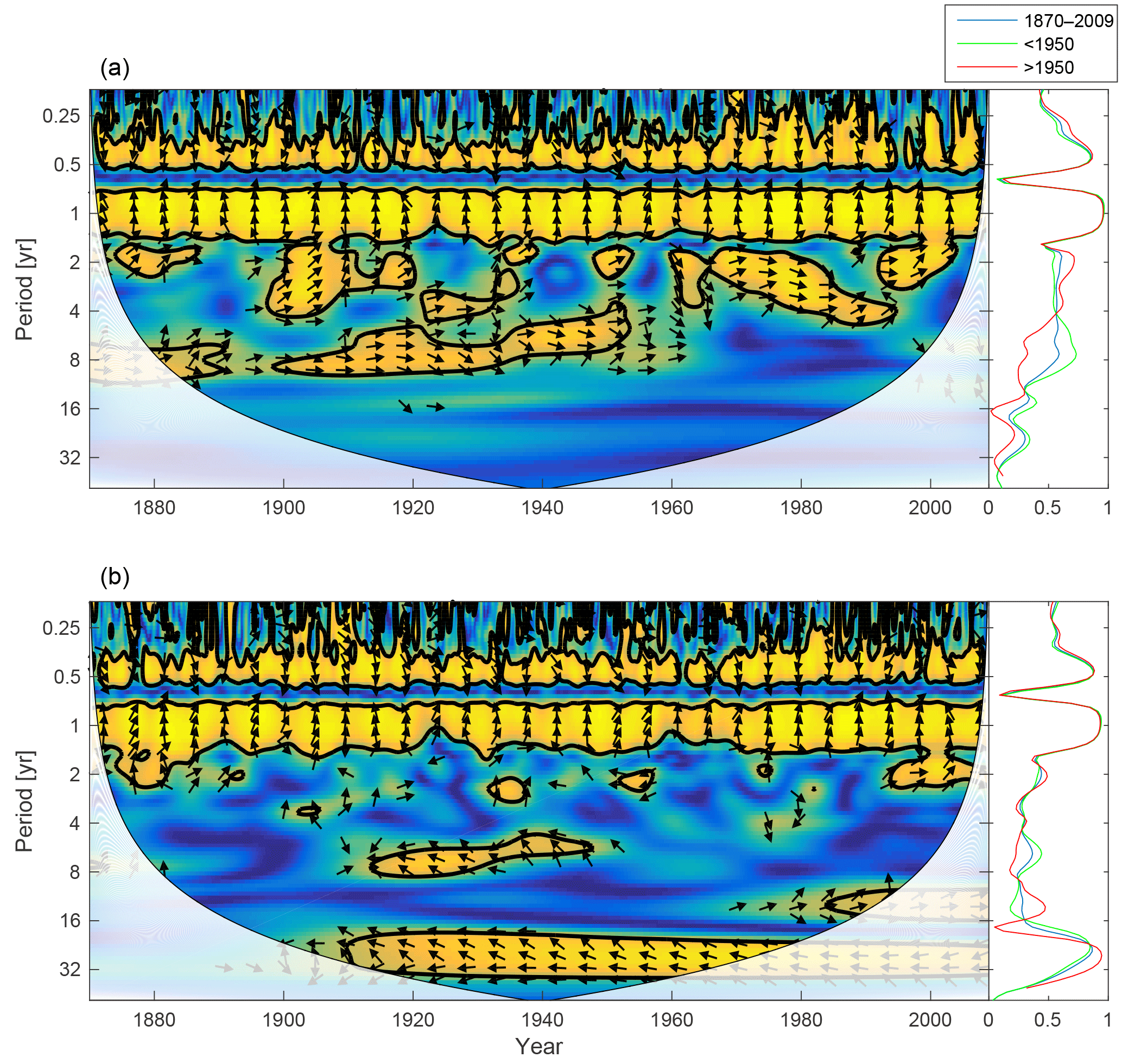
Figure 15Wavelet coherence between mixed-layer salinity and phosphate concentration (a) and mixed-layer salinity and DIN (b). Arrows pointing downwards indicate salinity preceding mixed-layer phosphate ∕ DIN by 90∘, while arrows pointing upwards mean mixed-layer phosphate ∕ DIN preceding salinity by the same amount. The right panels show the coherence averaged over the whole period (blue) and before (green) and after (red) 1950.
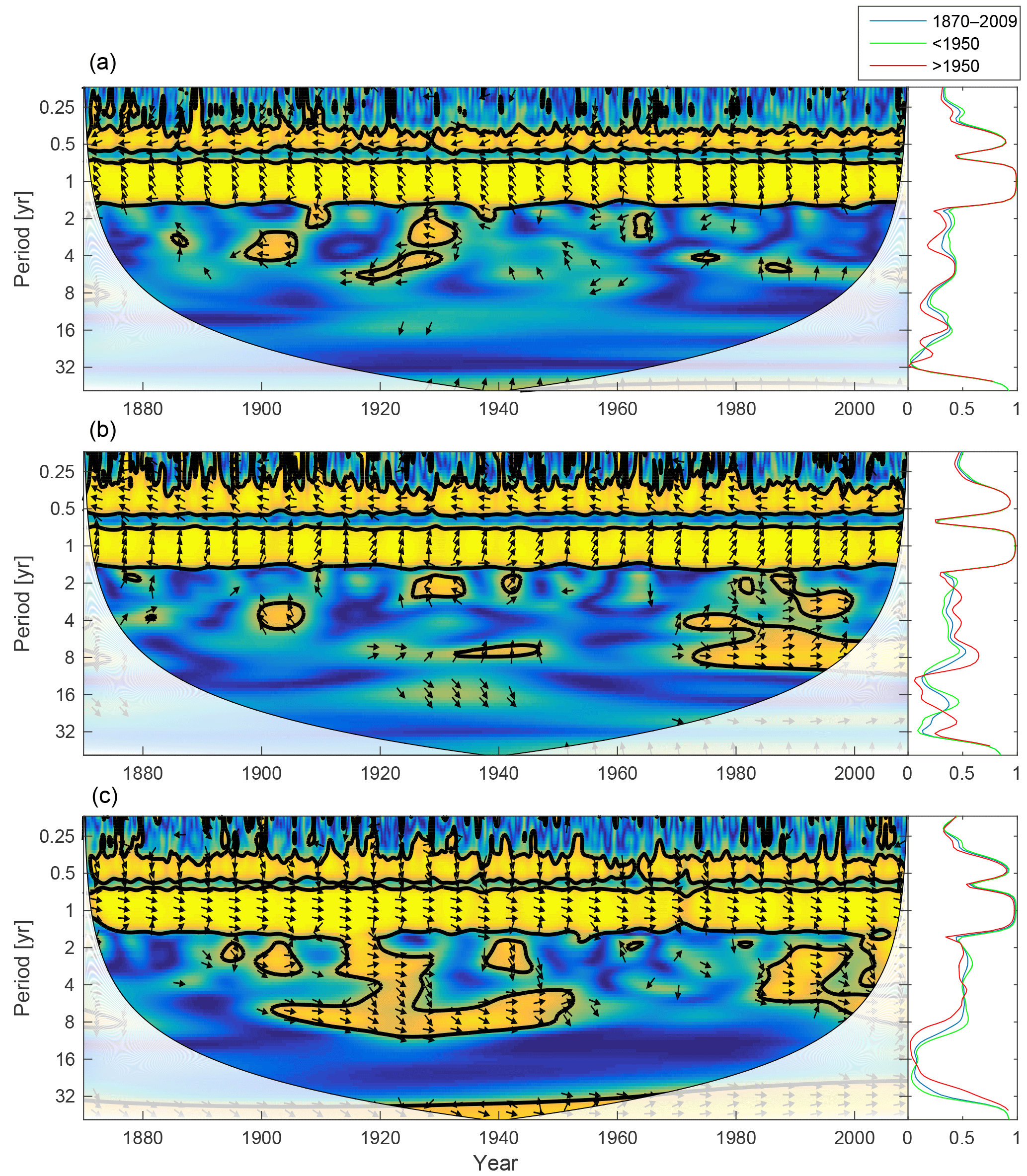
Figure 16Wavelet coherence between mixed-layer temperature and diatoms (a), flagellates (b) and cyanobacteria (c). Arrows pointing downwards indicate temperature preceding plankton group by 90∘, while arrows pointing upwards mean plankton preceding temperature by the same amount. The right panels show the coherence averaged over the whole period (blue) and before (green) and after (red) 1950.
The wavelet coherence between mixed-layer nutrients and riverine input is shown in Fig. 14. The phosphate concentration shows little coherence in periodicities longer than 1 year, but DIN displays strong inter-annual coherence. The phase arrows indicate a phase lag of about −45∘ on all inter-annual periodicities. For an 8-year period this means that a change in riverine input precedes changes in mixed-layer DIN by about 1 year.

Figure 17Wavelet coherence between mixed-layer depth and diatoms (a), flagellates (b) and cyanobacteria (c). Arrows pointing downwards indicate mixed-layer depth preceding plankton group by 90∘, while arrows pointing upwards mean plankton preceding mixed-layer depth by the same amount. The right panels show the coherence averaged over the whole period (blue) and before (green) and after (red) 1950.
To further investigate the lack of inter-annual coherence between riverine phosphate loads and the mixed-layer phosphate concentration, the wavelet coherence between mixed-layer salinity and nutrients is examined and displayed in Fig. 15. Mixed-layer salinity is affected by freshwater input from land, water exchange with adjacent basins, precipitation, evaporation and mixing with deeper layers. For periodicities spanning 1 to 16 years, the coherence spectrum reveals higher coherence between mixed-layer salinity and phosphate (top) than between salinity and DIN (bottom).
The coherence that does exist between salinity and DIN in periodicities longer than 1 year is anti-phase; i.e. low salinity here coheres with high DIN concentrations. This indicates that high runoff is connected to high nitrogen loads and high DIN concentrations in the mixed layer. It is also possible that low salinity in the mixed layer indicates periods with deep mixing and better oxygen conditions in and below the halocline (Stigebrandt and Gustafsson, 2007). This could reduce the denitrification during these periods and thus result in higher mixed-layer DIN concentrations.
In contrast, the stronger inter-annual in-phase coherence between salinity and phosphate suggests that the reason for the coherence might be a greater importance of phosphorus release from the sediments that eventually reaches the mixed layer through mixing with deeper layers (Eilola et al., 2014).
Riverine nutrient loads show little inter-annual coherence with phytoplankton biomass (not shown) other than in a 16 year period which probably reflects the overall pattern of simultaneous increase in riverine loads and phytoplankton biomass over the second half of the 20th century.
3.4 Temperature and irradiance
The mixed-layer temperature in the Baltic proper has increased over the 20th century. To analyse the effect of temperature on the phytoplankton biomass, the wavelet coherence between temperature and phytoplankton has been plotted in Fig. 16. The results suggest that the temperature increase after 1990 might have had an effect on cyanobacteria and flagellates. It is also noticeable that the temperature increase observed between 1900 and 1940 probably had an effect on cyanobacteria. This is also in agreement with the model formulation, where cyanobacteria are the most sensitive to temperature, followed by flagellates.
Light impacts primary production through the term LTLIM in Eq. (1). However, irradiance displays very little variation in any other periodicity than the annual one, as can be observed in a wavelet power spectrum (not shown). Therefore there exists almost no coherence between phytoplankton and irradiance apart from the seasonal signal.
3.5 Mixed-layer depth
We calculate the coherence between mixed-layer depth and diatoms, flagellates and cyanobacteria in Fig. 17.
Apart from the annual cycle there is a strong coherence between mixed-layer depth and diatoms, and to some extent flagellates, in shorter periodicities as well. That is, the diatom biomass residing in the mixed layer seems to co-vary quite well in periodicities equal to or shorter than 1 year. The model value for the diatom sinking rate is 5 times higher than that for flagellates, while cyanobacteria is assumed to have no sinking rate. In a shallow mixed layer the diatom biomass decreases faster than in a deep mixed layer because of the large sinking rate. Furthermore, in a deeper mixed layer stronger turbulence counteracts the sinking. In the wavelet coherence spectrum we thus see short-term in-phase coherence.
With a focus on simulated inter-annual variations, the wavelet coherence of the mixed-layer phytoplankton biomass with key variables affecting the primary production has been examined for the Baltic proper.
The simulated chlorophyll concentration maximum shifted from spring to late summer at the end of the 20th century in agreement with Kahru et al. (2016).
The phytoplankton group most strongly limited by nutrients in the model is diatoms. The connection between phytoplankton biomass and nutrients is reflected in the strong inter-annual coherence between diatoms and phosphate as well as NUTLIM before 1940. After 1940, NUTLIM and the biomass of individual phytoplankton groups increased to such an extent that inter-annual variations are small compared to the seasonal signal. Similarly, flagellates, which are less limited by nutrients than diatoms, show much smaller inter-annual coherence with phosphate even before 1940. NUTLIM for this group is high enough that small long-term variations are not reflected strongly in the results.
Very little inter-annual coherence is observed also between phytoplankton and DIN. Using the model's definition of nutrient limitation, the spring bloom is phosphate limited throughout the run except for a few years after 1990 in which diatoms are limited by nitrogen. Calculating instead limitation as given by mixed-layer N ∕ P ratios generates a pattern in line with previous estimates (Gustafsson et al., 2012; Savchuk et al., 2008; Schernewski and Neumann, 2004). The more prevalent phosphate limitation in the model is thus not a manifestation of incorrect N ∕ P ratios. Rather, it reflects a difference between the NUTLIM concept and N ∕ P ratios. NUTLIM is basically an efficiency, mapping a 3-D space made up of , and concentrations onto a value between 0 and 1. Limitations from N ∕ P ratios, meanwhile, are a 2-D mapping from and DIN onto a boolean variable.
We found strong coherence between riverine input of DIN and mixed-layer DIN but not a similar relationship between riverine phosphate input and the corresponding mixed-layer concentration. As mixed-layer salinity displayed inter-annual in-phase coherence with phosphate and only weak anti-phase coherence with DIN, we hypothesize that this is due to a greater importance of the flux of phosphate from lower layers.
The mixed-layer temperature in the Baltic proper has increased during the 20th century. We found some response of this mainly from the most-temperature-sensitive phytoplankton group cyanobacteria during periods of large inter-annual temperature increases. Flagellates, being more temperature sensitive than diatoms, seem to display a coherence with the temperature increase occurring after 1980.
Variations in mixed-layer depth mainly affects diatoms as these have a high sinking velocity. In-phase coherence between diatoms and mixed-layer depth in periodicities shorter than 1 year indicates that large seasonal changes in the mixed-layer depth significantly affect the mixed-layer diatom biomass, while smaller inter-annual variations are of little consequence.
Finally, inter-annual variations in irradiance have little effect on phytoplankton biomass accumulation.
The model data on which the results in the present study are based are stored by and available from the Swedish Meteorological and Hydrological Institute (https://www.smhi.se/, last access: 30 July 2018). Please send your request to ocean.data@smhi.se.
JH designed the study together with KE and MH. JH conducted all analysis and wrote the main part of the manuscript with contributions from KE, MH, HEMM and SS. BK provided the observational data.
The authors declare that they have no conflict of interest.
This work was funded by the Swedish Research Council (VR) within the project “Reconstruction and projecting Baltic Sea climate variability 1850–2100” (grant 2012-2117).
Funding was also provided by the Swedish Research Council for Environment, Agricultural Sciences and Spatial Planning (FORMAS) within the project “Cyanobacteria life cycles and nitrogen fixation in historical reconstructions and future climate scenarios (1850-2100) of the Baltic Sea” (grant no. 214-2013-1449). The study contributes also to the BONUS BalticAPP (Well-being from the Baltic Sea – applications combining natural science and economics) project, which has received funding from BONUS, the joint Baltic Sea research and development programme.
This research is also part of the BIO-C3 project and has received funding from BONUS (Art 185), funded jointly by the European Union's Seventh Framework Programme for research, technological development and demonstration and by national funding institutions.
We thank the associate editor and two anonymous referees for their insightful
comments and suggestions, which greatly improved the manuscript.
Edited by: Christine Klaas
Reviewed by: three
anonymous referees
Almroth-Rosell, E., Eilola, K., Meier, H. E. M., and Hall, P. O. J.: Transport of fresh and resuspended particulate organic material in the Baltic Sea – a model study, J. Marine Syst., https://doi.org/10.1016/j.jmarsys.2011.02.005, 2011. a, b
Carey, C. C., Hanson, P. C., Lathrop, R. C., and St. Amand, A. L.: Using wavelet analyses to examine variability in phytoplankton seasonal succession and annual periodicity, J. Plankton Res., 38, 27–40, https://doi.org/10.1093/plankt/fbv116, 2016. a, b, c
Carstensen, J., Andersen, J. H., Gustafsson, B. G., and Conley, D. J.: Deoxygenation of the Baltic Sea during the last century, P. Natl. Acad. Sci. USA, 111, 5628–5633, https://doi.org/10.1073/pnas.1323156111, 2014. a, b
Cazelles, B., Chavez, M., Berteaux, D., Ménard, F., Vik, J. O., Jenouvrier, S., and Stenseth, N. C.: Wavelet analysis of ecological time series, Oecologia, 156, 287–304, https://doi.org/10.1007/s00442-008-0993-2, 2008. a, b
Conley, D. J., Humborg, C., Rahm, L., Savchuk, O. P., and Wulff, F.: Hypoxia in the Baltic Sea and Basin-Scale Changes in Phosphorus Biogeochemistry, Environ. Sci. Technol., 36, 5315–5320, https://doi.org/10.1021/es025763w, 2002. a, b
Dortch, Q.: The interaction between ammonium and nitrate uptake in phytoplankton, Mar. Ecol.-Prog. Ser., 61, 183–201, https://doi.org/10.3354/meps061183, 1990. a
Droop, M.: Some thoughts on nutrient limitation in algae, J. Phycol., 9, 264–272, https://doi.org/10.1111/j.1529-8817.1973.tb04092.x, 1973. a
Eilola, K., Meier, H. E. M., and Almroth, E.: On the dynamics of oxygen, phosphorus and cyanobacteria in the Baltic Sea; A model study, J. Marine Syst., 75, 163–184, https://doi.org/10.1016/j.jmarsys.2008.08.009, 2009. a, b, c, d, e
Eilola, K., Gustafsson, B. G., Kuznetsov, I., Meier, H. E. M., Neumann, T., and Savchuk, O. P.: Evaluation of biogeochemical cycles in an ensemble of three state-of-the-art numerical models of the Baltic Sea, J. Marine Syst., 88, 267–284, https://doi.org/10.1016/j.jmarsys.2011.05.004, 2011. a
Eilola, K., Mårtensson, S., and Meier, H. E. M.: Modeling the impact of reduced sea ice cover in future climate on the Baltic Sea biogeochemistry, Geophys. Res. Lett., 40, 149–154, https://doi.org/10.1029/2012GL054375, 2013. a
Eilola, K., Almroth-Rosell, E., and Meier, H. E. M.: Impact of saltwater inflows on phosphorus cycling and eutrophication in the Baltic Sea: a 3D model study, Tellus A, 66, 1, https://doi.org/10.3402/tellusa.v66.23985, 2014. a, b
Flynn, K. J.: Ecological modelling in a sea of variable stoichiometry: Dysfunctionality and the legacy of Redfield and Monod, Prog. Oceanogr., 84, 52–65, https://doi.org/10.1016/j.pocean.2009.09.006, 2010. a
Fransner, F., Gustafsson, E., Tedesco, L., Vichi, M., Hordoir, R., Roquet, F., Spilling, K., Kuznetsov, I., Eilola, K., Mörth, C., Humborg, C., and Nycander, J.: Non-Redfieldian Dynamics Explain Seasonal pCO2 Drawdown in the Gulf of Bothnia, J. Geophys. Res.-Oceans, 123, 166–188, https://doi.org/10.1002/2017JC013019, 2018. a
Graham, L. P.: Modeling runoff to the Baltic Sea, Ambio, 28, 328–334, 1999. a
Granéli, E., Wallström, K., Larsson, U., Granéli, W., and Elmgren, R.: Nutrient limitation of primary production in the Baltic Sea Area, Ambio, 19, 142–151, 1990. a, b
Grinsted, A., Moore, J. C., and Jevrejeva, S.: Application of the cross wavelet transform and wavelet coherence to geophysical time series, Nonlin. Processes Geophys., 11, 561–566, https://doi.org/10.5194/npg-11-561-2004, 2004. a, b, c, d, e
Gustafsson, B. G., Schenk, F., Blenckner, T., Eilola, K., Meier, H. E. M., Müller-Karulis, B., Neumann, T., Ruoho-Airola, T., Savchuk, O. P., and Zorita, E.: Reconstructing the development of baltic sea eutrophication 1850–2006, Ambio, 41, 534–548, https://doi.org/10.1007/s13280-012-0318-x, 2012. a, b, c, d, e, f
Hansson, D., Eriksson, C., Omstedt, A., and Chen, D.: Reconstruction of river runoff to the Baltic Sea, AD 1500–1995, Int. J. Climatol., 31, 696–703, https://doi.org/10.1002/joc.2097, 2011. a
HELCOM: Approaches and methods for eutrophication target setting in the Baltic Sea region, Balt. Sea Env. Proc. No. 133, Helsinki Commision, Helsinki, 2012. a
Hense, I. and Beckmann, A.: The representation of cyanobacteria life cycle processes in aquatic ecosystem models, Ecol. Model., 221, 2330–2338, https://doi.org/10.1016/j.ecolmodel.2010.06.014, 2010. a
Jackett, D. R., McDougall, T. J., Feistel, R., Wright, D. G., and Griffies, S. M.: Algorithms for density, potential temperature, conservative temperature, and the freezing temperature of seawater, J. Atmos. Ocean. Tech., 23, 1709–1728, https://doi.org/10.1175/JTECH1946.1, 2006. a
Jakobsen, H. H. and Markager, S.: Carbon-to-chlorophyll ratio for phytoplankton in temperate coastal waters: Seasonal patterns and relationship to nutrients, Limnol. Oceanogr., 61, 1853–1868, https://doi.org/10.1002/lno.10338, 2016. a
Kahru, M., Elmgren, R., and Savchuk, O. P.: Changing seasonality of the Baltic Sea, Biogeosciences, 13, 1009–1018, https://doi.org/10.5194/bg-13-1009-2016, 2016. a, b, c
Lau, K. and Weng, H.: Climate signal detection using wavelet transform: How to make a time series sing, B. Am. Meteorol. Soc., 76, 2391–2402, https://doi.org/10.1175/1520-0477(1995)076<2391:csduwt>2.0.co;2, 1995. a
Meier, H. E. M. and Kauker, F.: Modeling decadal variability of the Baltic Sea: 2. Role of freshwater inflow and large-scale atmospheric circulation for salinity, J. Geophys. Res., 108, 1–16, https://doi.org/10.1029/2003JC001799, 2003. a
Meier, H. E. M., Döscher, R., and Faxén, T.: A multiprocessor coupled ice- ocean model for the Baltic Sea: application to the salt inflow, J. Geophys. Res., 108, 3273, https://doi.org/10.1029/2000JC000521, 2003. a, b
Meier, H. E. M., Andersson, H. C., Arheimer, B., Blenckner, T., Chubarenko, B., Donnelly, C., Eilola, K., Gustafsson, B. G., Hansson, A., Havenhand, J., Höglund, A., Kuznetsov, I., MacKenzie, B. R., Müller-Karulis, B., Neumann, T., Niiranen, S., Piwowarczyk, J., Raudsepp, U., Reckermann, M., Ruoho-Airola, T., Savchuk, O. P., Schenk, F., Schimanke, S., Väli, G., Weslawski, J.-M., and Zorita, E.: Comparing reconstructed past variations and future projections of the Baltic Sea ecosystem – first results from multi-model ensemble simulations, Environ. Res. Lett., 7, 034005, https://doi.org/10.1088/1748-9326/7/3/034005, 2012. a
Meier, H. E. M., Höglund, A., Eilola, K., and Almroth-Rosell, E.: Impact of accelerated future global mean sea level rise on hypoxia in the Baltic Sea, Clim. Dynam., 49, 163–172, https://doi.org/10.1007/s00382-016-3333-y, 2017. a
Meier, H. E. M., Eilola, K., Almroth-Rosell, E., Schimanke, S., Kniebusch, M., Höglund, A., Pemberton, P., Liu, Y., Väli, G., and Saraiva, S.: Disentangling the impact of nutrient load and climate changes on Baltic Sea hypoxia and eutrophication since 1850, Clim. Dynam., https://doi.org/10.1007/s00382-018-4296-y, 2018a. a, b
Meier, H. E. M., Väli, G., Naumann, M., Eilola, K., and Frauen, C.: Recently accelerated oxygen consumption rates amplify deoxygenation in the Baltic Sea., J. Geophys. Res., 123, 3227–3240, https://doi.org/10.1029/2017JC013686, 2018b. a
Menden-Deuer, S. and Lessard, E. J.: Carbon to volume relationships for dinoflagellates, diatoms, and other protist plankton, American Society of Limnology and Oceanography, 3, 569–579, https://doi.org/10.4319/lo.2000.45.3.0569, 2000. a
Parker, R. A.: Dynamic models for ammonium inhibition of nitrate uptake by phytoplankton, Ecol. Model., 66, 113–120, https://doi.org/10.1016/0304-3800(93)90042-Q, 1993. a
Rakko, A. and Seppälä, J.: Effect of salinity on the growth rate and nutrient stoichiometry of two Baltic Sea filamentous cyanobacterial species, Estonian Journal of Ecology, 63, 55–70, https://doi.org/10.3176/eco.2014.2.01, 2014. a
Redfield, A. C.: The biological control of chemical factors in the environment, Am. Sci., 46, 205–221, 1958. a
Ruoho-Airola, T., Eilola, K., Savchuk, O. P., Parviainen, M., and Tarvainen, V.: Atmospheric nutrient input to the baltic sea from 1850 to 2006: A reconstruction from modeling results and historical data, Ambio, 41, 549–557, https://doi.org/10.1007/s13280-012-0319-9, 2012. a
Savchuk, O. P.: Large-Scale Dynamics of Hypoxia in the Baltic Sea, in: Chemical structure of pelagic redox interfaces: Observation and modeling, Hdb Env Chem, edited by: Yakushev, E. V., 137–160, Springer-Verlag, Berlin Heidelberg, https://doi.org/10.1007/698_2010_53, 2010. a, b
Savchuk, O. P.: Large-Scale Nutrient Dynamics in the Baltic Sea, 1970–2016, Frontiers in Marine Science, 5, 95, https://doi.org/10.3389/fmars.2018.00095, 2018. a
Savchuk, O. P., Wulff, F., Hille, S., Humborg, C., and Pollehne, F.: The Baltic Sea a century ago – a reconstruction from model simulations, verified by observations, J. Marine Syst., 74, 485–494, https://doi.org/10.1016/j.jmarsys.2008.03.008, 2008. a, b, c, d, e
Savchuk, O. P., Gustafsson, B. G., Rodríguez, M., Sokolov, A. V., and Wulff, F. V.: External nutrient loads to the Baltic Sea, 1970–2006, Technical report no. 5, Baltic Nest Institute, Stockholm, 2012. a, b
Schernewski, G. and Neumann, T.: The trophic state of the Baltic Sea a century ago: a model simulation study, J. Marine Syst., 53, 109–124, https://doi.org/10.1016/j.jmarsys.2004.03.007, 2004. a, b, c
Schimanke, S. and Meier, H.: Decadal to centennial variability of salinity in the Baltic Sea, J. Climate, 29, 7173–7188, https://doi.org/10.1175/JCLI-D-15-0443.1, 2016. a
Stigebrandt, A. and Gustafsson, B. G.: Improvement of Baltic Proper Water Quality Using Large-scale Ecological Engineering, Ambio, 36, 280–286, https://doi.org/10.1579/0044-7447(2007)36[280:IOBPWQ]2.0.CO;2, 2007. a
Tamminen, T. and Andersen, T.: Seasonal phytoplankton nutrient limitation patterns as revealed by bioassays over Baltic Sea gradients of salinity and eutrophication, Mar. Ecol.-Prog. Ser., 340, 121–138, https://doi.org/10.3354/meps340121, 2007. a
Torrence, C. and Compo, G. P.: A practical guide to wavelet analysis, B. Am. Meteorol. Soc., 79, 61–78, https://doi.org/10.1175/1520-0477(1998)079<0061:APGTWA>2.0.CO;2, 1998. a, b
Vahtera, E., Conley, D. J., Gustafsson, B. G., Kuosa, H., Pitkanen, H., Savchuk, O. P., Tamminen, T., Viitasalo, M., Wasmund, N., and Wulff, F.: Internal Ecosystem Feedbacks Enhance Nitrogen-fixing Cyanobacteria, Ambio, 36, 186–193, 2007. a, b, c
Winder, M. and Cloern, J. E.: The annual cycles of phytoplankton biomass, Philos. T. Roy. Soc. B, 365, 3215–3226, https://doi.org/10.1098/rstb.2010.0125, 2010. a, b