The impact of spatiotemporal variability in atmospheric CO₂ concentration on global terrestrial carbon fluxes

Land carbon fluxes, e.g., gross primary production (GPP) and net biome production (NBP), are controlled in part by the responses of terrestrial ecosystems to atmospheric conditions near the Earth's surface. The Coupled Model Intercomparison Project Phase 6 (CMIP6) has recently proposed increased spatial and temporal resolutions for the surface CO₂ concentrations used to calculate GPP, and yet a comprehensive evaluation of the consequences of this increased resolution for carbon cycle dynamics is missing. Here, using global offline simulations with a terrestrial biosphere model, the sensitivity of terrestrial carbon cycle fluxes to multiple facets of the spatiotemporal variability in atmospheric CO₂ is quantified. Globally, the spatial variability in CO₂ is found to increase the mean global GPP by a maximum of 0.05 Pg C year⁻¹, as more vegetated land areas benefit from higher CO₂ concentrations induced by the inter-hemispheric gradient. The temporal variability in CO₂, however, compensates for this increase, acting to reduce overall global GPP; in particular, consideration of the diurnal variability in atmospheric CO₂ reduces multi-year mean global annual GPP by 0.5 Pg C year⁻¹ and net land carbon uptake by 0.1 Pg C year⁻¹. The relative contributions of the different facets of CO₂ variability to GPP are found to vary regionally and seasonally, with the seasonal variation in atmospheric CO₂, for example, having a notable impact on GPP in boreal regions during fall. Overall, in terms of estimating global GPP, the magnitudes of the sensitivities found here are minor, indicating that the common practice of applying spatially uniform and annually increasing CO₂ (without higher-frequency temporal variability) in offline studies is a reasonable approach – the small errors induced by ignoring CO₂ variability are undoubtedly swamped by other uncertainties in the offline calculations. Still, for certain regional- and seasonal-scale GPP estimations, the proper treatment of spatiotemporal CO₂ variability appears important.

1 Introduction

Quantifying the sources and sinks of carbon at the land surface is key to an accurate carbon balance and to the overall assessment of where anthropogenically released fossilized carbon ends up in the Earth system. While current estimates suggest that the land absorbs the equivalent of about a quarter of anthropogenic CO₂ emissions (IPCC, 2014), the uncertainty in the global carbon budget associated with terrestrial ecosystem processes is large (Le Quéré et al., 2016). For example, studies disagree on the partitioning of the land carbon sink between the tropics and the extratropics. Some studies consider tropical ecosystems to be carbon sinks (Stephens et al., 2007; Lewis et al., 2009; Schimel et al., 2015) and others consider them to be carbon sources (Baccini et al., 2017; Houghton et al., 2018). A substantial interannual variability is found in the tropical carbon balance, primarily in response to climate-driven variations (Baker et al., 2006; Cleveland et al., 2015; Fu et al., 2017); indeed, tropical ecosystems represent a large fraction of the uncertainty in estimates of the total land carbon sink and its future trajectory (Pan et al., 2011; Wang et al., 2014). Carbon fluxes in boreal ecosystems also remain highly uncertain and are likely to be strongly influenced by changes in climate and the length of growing season. Warming over northern lands may lead to an increase in vegetation productivity (Xu et al., 2013) and to a greater amplitude of seasonal CO₂ exchange (Forkel et al., 2016) via climate-induced changes in phenological seasonal cycles (e.g., earlier vegetation “green-up”).

Because terrestrial carbon dynamics are greatly influenced by atmospheric forcing (e.g., air temperature, precipitation, radiation, humidity, CO₂ concentration), quantifying the sensitivity of surface carbon fluxes to variations in atmospheric drivers is critical to obtaining accurate flux estimates. Such quantification helps identify model processes and assumptions that are responsible for the uncertainty. It indeed promotes essential understanding regarding what controls these fluxes, understanding that should, in turn, lead to improved models of terrestrial carbon processes. Only with accurate models can we obtain reasonably accurate projections of climate under different emission scenarios.

While the impacts of some aspects of atmospheric variability, such as that of temperature and precipitation, on global land carbon fluxes have been explored extensively (e.g., Beer et al., 2010; Poulter et al., 2014; Ahlström et al., 2015), the impact of atmospheric CO₂ variability on the fluxes is relatively understudied and is in fact generally ignored in recent flux estimation exercises. In most land surface model (LSM) or terrestrial biosphere model (TBM) simulations, the atmospheric CO₂ applied is annually and/or spatially uniform (e.g., TRENDY project; Sitch et al., 2015) or allowed to vary only on a monthly and/or zonal basis (e.g., Multi-scale Terrestrial Model Intercomparison Project (MsTMIP); Huntzinger et al., 2013; Wei et al., 2014; Ito et al., 2016). Potential time variations in the carbon fluxes associated with the diurnal and day-to-day variability, if monthly CO₂ is applied, and also with the seasonal variability, if annual CO₂ is applied, are not represented in these modeling studies. Likewise, the regional flux response to spatial variations in CO₂ is only partially represented with the latitudinal CO₂ driver and not at all with the spatially uniform CO₂ driver.

Such simplifications neglect lessons from decades of in situ measurements showing that CO₂ concentrations vary widely on different time and space scales. During the growing season, daytime (nighttime) CO₂ at the canopy level can be significantly smaller (larger) than the daily mean CO₂ due to the diurnal cycle of photosynthesis. Summertime measurements, for example, at an 11 m tower in northern Wisconsin indicate that the atmospheric CO₂ concentration fluctuates by approximately 70 ppm over the course of a day, from 350 ppm during the day to 420 ppm at night (Yi et al., 2000); indeed, the day–night difference is comparable to the global atmospheric CO₂ growth of the last few decades (∼63 ppm since 1980). In addition to large diurnal variations, many stations observe strong seasonal variations in CO₂ concentrations; for example, such variations are as large as 30 ppm at the Hegyhátsál monitoring site in western Hungary (e.g., Haszpra et al., 2008).

Spatial variations in CO₂ are also known to be significant. Concentrations of CO₂ contain large spatial gradients with higher annual mean values found in the Northern Hemisphere than in the Southern Hemisphere due to the higher level of fossil fuel emissions (Tans et al., 1989). Higher annual mean concentrations are evident over land masses, particularly those with large anthropogenic emissions. In addition, the covariance between flux processes and atmospheric transport results in a phenomenon called the “rectifier effect” wherein substantial spatial variations are introduced into simulated CO₂ fields, even when an annually balanced biosphere flux is assumed (Denning et al., 1995, 1999).

In light of such known variations, the Coupled Model Intercomparison Project (CMIP6) is now encouraging modeling groups to force their offline models with CO₂ concentrations that vary in space and time (Eyring et al., 2016). Ostensibly this makes sense, given that relevant datasets on temporal and spatial CO₂ variations are available for use (Meinshausen et al., 2017). Nevertheless, it seems appropriate at the outset of such efforts to quantify the potential usefulness of this added complexity. It is still arguably unknown how much the uncertainty in estimated terrestrial carbon fluxes will decrease through the explicit consideration of CO₂ variations.

In a recent study, Liu et al. (2016) begin to address this issue – they use a TBM to show that the explicit consideration of the seasonal variation in CO₂ in modeling studies can lower the estimated terrestrial gross primary production (GPP) by 0.4 Pg C year⁻¹ globally, and they also show that the consideration of the spatial variability in CO₂ can increase mean global GPP estimates by 2.1 Pg C year⁻¹. There are, however, additional facets of CO₂ variability that are worth exploring. In particular, diurnal variations in CO₂ are known to be large (e.g., ∼70 ppm in the central US and ∼50 ppm in central Europe), and it is worth determining if, in ignoring these particular variations, process-based models produce significant errors in carbon flux estimation.

In this paper we provide an analysis of carbon flux sensitivity to spatial and temporal variations in atmospheric CO₂ that is duly comprehensive. We employ in this study a particular process-based terrestrial biosphere model, the Catchment-CN model of NASA's Global Modeling and Assimilation Office (GMAO). We first evaluate the ability of the model to reproduce observationally informed carbon flux estimates. This evaluation includes a test of our model's response to artificially enriched CO₂ – an imposed surplus of 200 ppm, mimicking the surplus applied in an established field experiment. Then, in a carefully designed suite of simulation experiments, we quantify the sensitivity of monthly simulated GPP and net biome production (NBP) to different temporal and spatial scales of atmospheric CO₂ variability. The paper concludes with some discussion on the implications of the results for future carbon cycle research.

2 Methods

2.1 Catchment-CN model

The NASA Catchment-CN model (Koster et al., 2014) is a hybrid of two existing models: the NASA Catchment model (Koster et al., 2000) and the NCAR Community Land Model version 4 (CLM4) (Oleson et al., 2010). The hybrid utilizes the code from the Catchment model that performs water and energy budget calculations. The carbon and nitrogen dynamics from CLM4 provides to the hybrid all of the carbon reservoir and carbon flux calculations as well as photosynthesis-based estimates of canopy conductance for use in the Catchment model's energy balance equations. Unlike most land surface models, the surface element for Catchment-CN is the hydrological catchment (with a typical spatial dimension of about 20 km); model equations further provide a separation of each catchment into three separate dynamic hydrological regimes, each with its own set of energy balance calculations. There are 19 available plant functional types (PFTs) (Table S1 in the Supplement), and up to four PFTs are allowed in each of three static sub-areas loosely tied to the three hydrological regimes. The model used a 10 min time step for the energy and water balance calculations and a 90 min time step for the carbon calculations. This model's ability to capture the observed sensitivity of phenological variables to moisture variations was demonstrated in Koster et al. (2014).

The environmental variables (temperature, precipitation, radiation, humidity, wind and atmospheric CO₂ concentrations) directly affect leaf photosynthesis (A) in Catchment-CN (as in NCAR CLM4 (Oleson et al., 2010); see also Farquhar et al. (1980) and Collatz et al. (1991) for the C₃ plant model, and Collatz et al. (1992) for the C₄ plant model), which is predicted to be the minimum value (Eq. 1) of Rubisco-limited photosynthesis (ω_c, Eq. 2), light-limited photosynthesis (ω_j, Eq. 3) and export-limited photosynthesis (ω_e, Eq. 4):

$$\begin{array}{}\text{(1)}& {\displaystyle }& {\displaystyle }A=min\left({\mathit{\omega }}_c,{\mathit{\omega }}_j,{\mathit{\omega }}_e\right),\text{(2)}& {\displaystyle }& {\displaystyle }{\mathit{\omega }}_c=\left\{\begin{array}{ll}{\displaystyle \frac{V_{\mathrm{cmax}}(c_{\mathrm{i}}-{\mathrm{\Gamma }}_{\ast })}{c_{\mathrm{i}}+K_{\mathrm{c}}(\mathrm{1}+\frac{o_{\mathrm{i}}}{K_{\mathrm{o}}})}}& \text{ for }{\mathrm{C}}_{\mathrm{3}}\text{ plants}\\ V_{\mathrm{cmax}}& \text{ for }{\mathrm{C}}_{\mathrm{4}}\text{ plants}\end{array}\right.,\text{(3)}& {\displaystyle }& {\displaystyle }{\mathit{\omega }}_j=\left\{\begin{array}{ll}{\displaystyle \frac{\left(c_i-{\mathrm{\Gamma }}_{\ast }\right)\mathrm{4.6}\mathit{\varphi }\mathit{\alpha }}{C_i+\mathrm{2}{\mathrm{\Gamma }}_{\ast }}}& \text{ for }{\mathrm{C}}_{\mathrm{3}}\text{ plants}\\ \mathrm{4.6}\mathit{\varphi }\mathit{\alpha }& \text{ for }{\mathrm{C}}_{\mathrm{4}}\text{ plants}\end{array}\right.,\text{(4)}& {\displaystyle }& {\displaystyle }{\mathit{\omega }}_e=\left\{\begin{array}{ll}\mathrm{0.5}{V}_{\mathrm{cmax}}& \text{ for }{\mathrm{C}}_{\mathrm{3}}\text{ plants}\\ \mathrm{4000}{V}_{\mathrm{cmax}}{\displaystyle \frac{c_{\mathrm{i}}}{P_{\mathrm{atm}}}}& \text{ for }{\mathrm{C}}_{\mathrm{4}}\text{ plants}\end{array}\right.,\end{array}$$

where c_i is the internal leaf CO₂ partial pressure (Pa) and o_i is the O₂ partial pressure (Pa). K_c and K_o are the Michaelis–Menten parameters (Pa) for CO₂ and O₂, respectively, and vary according to the leaf temperature. Γ_∗ is the CO₂ compensation point (Pa), α is quantum efficiency, ϕ is absorbed photosynthetically active radiation (APAR) (W m⁻²), and V_cmax is the maximum rate of carboxylation ($\mathrm{\mu }\mathrm{mol}{\mathrm{CO}}_{\mathrm{2}}{\mathrm{m}}^{-\mathrm{2}}{\mathrm{s}}^{-\mathrm{1}}$), which varies according to the leaf temperature, soil water and day length. Photosynthesis calculations of the type represented by Eqs. (1)–(4) are common in process-based LSMs, including, for example, the Joint UK Land Environment Simulator (JULES) model (Walters et al., 2014) and the Organising Carbon and Hydrology In Dynamic Ecosystems (ORCHIDEE) model (Krinner et al., 2005).

Leaf photosynthesis ($\mathrm{\mu }\mathrm{mol}{\mathrm{CO}}_{\mathrm{2}}{\mathrm{m}}^{-\mathrm{2}}{\mathrm{s}}^{-\mathrm{1}}$; denoted as A) can also be expressed in terms of the diffusion gradient and stomatal conductance for CO₂ among the ambient atmosphere, the leaf surface and the internal leaf:

$$\begin{array}{ll}{\displaystyle }A& {\displaystyle }={\displaystyle \frac{c_{\mathrm{a}}-c_{\mathrm{i}}}{\left(\mathrm{1.37}{r}_{\mathrm{b}}+\mathrm{1.65}{r}_{\mathrm{s}}\right)P_{\mathrm{atm}}}}\\ \text{(5a)}& {\displaystyle }& {\displaystyle }\left(\text{between atmosphere and internal leaf}\right),{\displaystyle }& {\displaystyle }={\displaystyle \frac{c_{\mathrm{a}}-c_{\mathrm{s}}}{\left(\mathrm{1.37}{r}_{\mathrm{b}}\right)P_{\mathrm{atm}}}}\\ \text{(5b)}& {\displaystyle }& {\displaystyle }\left(\text{between atmosphere and leaf surface}\right),{\displaystyle }& {\displaystyle }={\displaystyle \frac{c_{\mathrm{s}}-c_{\mathrm{i}}}{\left(\mathrm{1.65}{r}_{\mathrm{s}}\right)P_{\mathrm{atm}}}}\\ \text{(5c)}& {\displaystyle }& {\displaystyle }\left(\text{between leaf surface and internal leaf}\right),\end{array}$$

where r_b is boundary layer resistance and r_s is leaf stomatal resistance (m² s µmol⁻¹), and where c_a is the CO₂ partial pressure of ambient atmosphere and c_s is the pressure at leaf surface (note that Eq. 5a is a consequence of the others, Eq. 5b and c).

Using the Ball–Berry model of stomatal conductance (Ball et al., 1987; Collatz et al., 1991), r_s is expressed as a function of A, c_s and vapor pressures (e_s, the vapor pressure at the leaf surface, and e_i, the saturation vapor pressure inside the leaf):

$$\begin{array}{}\text{(6)}& {\displaystyle \frac{\mathrm{1}}{r_{\mathrm{s}}}}=m{\displaystyle \frac{A}{c_{\mathrm{s}}}}{\displaystyle \frac{e_{\mathrm{s}}}{e_{\mathrm{i}}}}{P}_{\mathrm{atm}}+b,\end{array}$$

where m is a parameter dependent upon PFT (m=5 for C₄ grass, 6 for needleleaf trees, and 9 for all other types), and b is the minimum stomatal conductance (20 000 $\mathrm{\mu }\mathrm{mol}{\mathrm{m}}^{-\mathrm{2}}{\mathrm{s}}^{-\mathrm{1}}$). Assuming the initial value of c_i to be 0.7 c_a (for C₃ plants) or 0.4 c_a (for C₄ plants), the Catchment-CN model simultaneously computes the leaf photosynthesis (A) from Eqs. (1)–(4). This value of A is then used to estimate c_s in Eq. (5b) and r_s in Eq. (6), as well as c_i in Eq. (5c), which is inserted back into Eqs. (2)–(4) for another calculation of A. The iteration cycle proceeds three times to obtain the final value of A. A grid-level GPP is tied directly to the computed photosynthesis by taking a tile-based (i.e., delineated catchment) area-weighted average of A.

NBP is calculated as

$$\begin{array}{}\text{(7)}& \mathrm{NBP}=\mathrm{GPP}-R_{\mathrm{a}}-R_{\mathrm{h}}-F,\end{array}$$

where R_a is the autotrophic respiration (through plant growth and maintenance), R_h is the heterotrophic respiration (through litter and soil decomposition) and F is fire carbon flux. Positive (negative) NBP values mean that the land surface is a carbon sink (source). The respiration terms R_a and R_h were calculated as in NCAR CLM4, except for a modification to R_h, imposed here, that prohibits decomposition if the soil water is frozen. With this modification, the Catchment-CN's NBP showed a better agreement with atmospheric inversion estimates in the northern high-latitude regions during December through February. The fire term (F) is controlled by the amount of available fuel and the status of soil moisture. Note that our study did not consider carbon flux changes associated with land use (e.g., deforestation).

2.2 Datasets for model evaluation and comparison

Given that no direct measurements of GPP exist at the global scale (Anav et al., 2015), we evaluate the GPP values produced in our control simulation against GPP estimates from the data-derived FLUXNET Multi-Tree Ensemble (MTE) GPP project (hereafter referred to as MTE-GPP) (https://www.bgc-jena.mpg.de/geodb/projects/Home.php, last access: May 2013). This global-scale, monthly, gridded dataset effectively consists of upscaled observations from the eddy-covariance towers of the FLUXNET network; the upscaling utilizes the the MTE approach with inputs of (i) meteorological data, (ii) the fraction of absorbed photosynthetically active radiation (fPAR) derived from the Global Inventory Modeling and Mapping Studies (GIMMS) normalized difference vegetation index (NDVI) and (iii) land cover information (i.e., vegetation type) (Jung et al., 2009, 2011). The flux partitioning method utilized was from Lasslop et al. (2010). This dataset is widely used for performance evaluation of TBMs including CLM (e.g., Bonan et al., 2011).

The net carbon fluxes (i.e., NBP) of the Catchment-CN model were evaluated against estimates from three atmospheric inversions: Monitoring Atmospheric Composition and Climate (MACC) v14r2 (Chevallier et al., 2011; http://macc.copernicus-atmosphere.eu/, last access: June 2017), CarbonTracker 2015 (Peters et al., 2007, with updates documented at http://carbontracker.noaa.gov, last access: August 2016) and Jena CarboScope v3.8 (Rödenbeck et al., 2003; http://www.bgc-jena.mpg.de/CarboScope/, last access: March 2017). The atmospheric inversion methods use atmospheric CO₂ concentration measurements in conjunction with an atmospheric transport model to provide a range of estimates of net carbon fluxes between the atmosphere and biosphere. The net carbon fluxes of the Catchment-CN model were also compared with fluxes estimated by the diagnostic Carnegie–Ames–Stanford Approach (CASA) Global Fire Emission Database (GFED, version 3) (Ott et al., 2015; van der Werf et al., 2010). CASA GFED3 is a widely used dataset that is heavily constrained by satellite observations, including GIMMS FPAR, as well as by MERRA-2 meteorology. The mean NBP of the 11 years (2004–2014) overlapping our control simulation were evaluated.

2.3 Experimental design

In all simulations examined in this study, the Catchment-CN model is driven with atmospheric fields from NASA's Modern-Era Retrospective analysis for Research and Applications, version 2 (MERRA-2) reanalysis (Gelaro et al., 2017, and also available at http://gmao.gsfc.nasa.gov/reanalysis/MERRA-2/, last access: August 2015). Since MERRA-2 fields are provided on a $\mathrm{0.5}{}^{\circ }\times \mathrm{0.625}{}^{\circ }$ resolution grid, the forcing values for a given Catchment-CN tile are taken from the MERRA-2 grid cell whose center is closest to the tile's centroid. Precipitation forcing is the same as that used in the production of the Soil Moisture Active Passive (SMAP) level 4 product (Reichle et al., 2016); this precipitation is scaled to agree with rain gauge observations where available.

Our control case imposes a maximum level of CO₂ variability. In the control simulation, the model is forced with time-varying (at 3-hourly resolution) and spatially varying (at 3^∘ longitude × 2^∘ latitude resolution) global fields of CO₂ concentration over the period 2001–2014. The surface CO₂ fields are extracted from the NOAA CarbonTracker database (Peters et al., 2007) for this period (CT2015, http://www.esrl.noaa.gov/gmd/ccgg/carbontracker/molefractions.php, last access: August 2016).

We achieved reasonable initial land carbon states for 1 January 2001 using a two-step approach. First, starting with carbon prognostic states already equilibrated over multiple millennia with a somewhat different modeling–forcing combination (including the use of present-day CO₂ concentrations), the Catchment-CN model was run for at least 2000 additional simulation years under a spatially and temporally uniform CO₂ concentration of 280 ppm to mimic the preindustrial era (i.e., before 1850), with meteorological forcing consisting of repeated cycles of the 1981–2015 MERRA-2 dataset. In the second step, the period from 1850 to 2000 was simulated using CO₂ concentrations that varied diurnally, seasonally, and spatially and that grew linearly in time to match the observed CO₂ conditions (see below). The meteorological forcing applied during this time was also the cycled 1981–2015 MERRA-2 forcing and thus was also not tied to true year-specific forcing (except for within the final 1981–2000 period); such meteorological information is unavailable for the earlier part of the industrial period, and in any case, the main point of the exercise was to allow the carbon reservoirs in the land surface to respond to the gradual increase in CO₂ concentrations. The resulting status of the land ecosystem on 1 January 2001 was used as the initial condition for the control simulation and for all experiments.

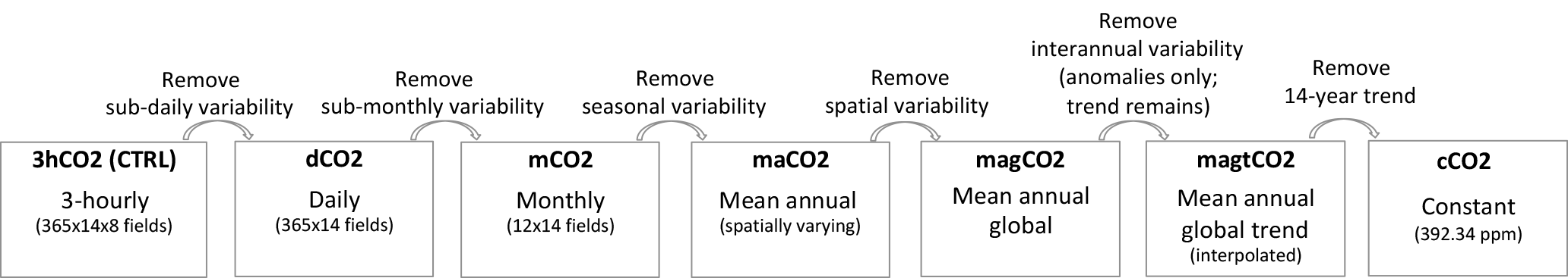
Figure 1 Schematic of the six simulations examined in this study, which were designed to isolate the impacts of the different facets' spatiotemporal CO₂ variability on simulated carbon fluxes. The CO₂ concentrations were reconstructed from the NOAA CarbonTracker 3-hourly global CO₂ data.

The CO₂ concentration fields used during the 1850–2000 spin-up period were constructed as follows. First, the 3-hourly, spatially varying CarbonTracker CO₂ fields were averaged over 2001–2014 and over each month into a climatological 3-hourly diurnal cycle for each of the 12 months of the year (i.e., 96 fields – eight 3-hourly fields for each month at each grid location). The 12 diurnal cycles were then assigned to the middle of each month and linear interpolation to each day of year produced 365 climatological diurnal cycles of CO₂ concentration. We applied these daily diurnal cycles in each year of 1850–2000 after scaling them with a year-specific scaling factor that forced the annual, global mean CO₂ concentration to increase linearly in time from 280 ppm in 1850 to 311 ppm in 1950 and then from this value to 375.5 ppm in 2000 (to approximate the growth in CO₂ seen in the historical record; see http://www.eea.europa.eu/data-and-maps/figures/atmospheric-concentration-of-co2-ppm-1, last access: April 2016). All of the interpolation was performed in the time dimension only; the global spatial variation contained within the CarbonTracker data was retained.

The strategy behind our experiments is described in Fig. 1. We performed a series of six experiments covering the period 2001–2014 (applying the same meteorology except for the atmospheric CO₂ concentrations and using the same 2001 initial conditions as the control), with each experiment removing, in turn, one facet of the spatiotemporal variability in atmospheric CO₂ concentration. In the first experiment (referred to as dCO2), the 3-hourly CO₂ diurnal cycle was averaged into a single daily value at every tile, and these daily-averaged values were then used to force the Catchment-CN model. Comparing the results of this experiment to those of the control thus illustrates the impact of ignoring diurnal CO₂ variability on the modeled carbon fluxes. In the second experiment (mCO2), day-to-day variability in CO₂ was removed – the daily CO₂ concentrations used in dCO2 were averaged into monthly values, which were then linearly interpolated (as in the spin-up procedure) into a temporally smoothed version of the daily fields. Note that through the interpolation, the global average of CO₂ is conserved in essence. In the third experiment (maCO2), seasonality in CO₂ was removed – the annual average CO₂ from CarbonTracker above a surface element was applied to that element. Note that the annual fields used for maCO2 still retain the spatial variability in CO₂ inherent in the CarbonTracker data; this spatial variability was removed in the fourth experiment (magCO2), in which the globally uniform but yearly varying mean annual CO₂ fields were used. This experiment (magCO2) replicates the commonly used CO₂ forcing fields applied in many other land modeling experiments. Finally, in the fifth and sixth experiments, different facets of the interannual variability in CO₂ were removed. In the fifth experiment (magtCO2), year-to-year variations in globally averaged CO₂ were removed while retaining the overall mean trend; this was achieved by regressing the 14 annual mean values used in magCO2 against the year index and then using the resulting regression line to assign the annual values. In the sixth experiment (cC02), the long-term trend was also removed by averaging the 14 annual values into a single number – in cCO2, a constant CO₂ concentration (392.34 ppm) was applied everywhere, every 10 min.

All of our analyses were performed on tile-based fluxes. This efficiently excludes coastal water and lake water impacts and thus allows for an accurate estimation of the aggregated land-based global carbon fluxes. We computed mean global GPP by multiplying tile-based fluxes (in units of $\mathrm{g}\mathrm{C}{\mathrm{m}}^{-\mathrm{2}}{\mathrm{s}}^{-\mathrm{1}}$) by the associated tile area and then aggregating the areal totals over global land (excluding Greenland and Antarctica). The mean global NBP was estimated in the same way.

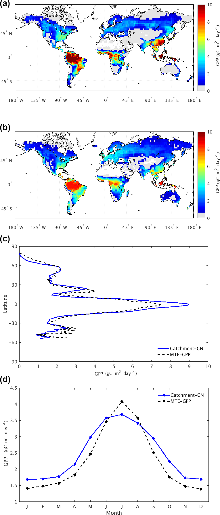
Figure 2 Spatial patterns of 2002–2011 mean GPP ($\mathrm{g}\mathrm{C}{\mathrm{m}}^{-\mathrm{2}}{\mathrm{day}}^{-\mathrm{1}}$) from (a) Catchment-CN GPP and (b) MTE-GPP as well as (c) zonal mean GPP and (d) the annual cycle of GPP (solid blue: Catchment-CN model; dotted black: MTE-GPP).

3 Results

We evaluate in Sect. 3.1 and 3.2 the ability of the control simulation to produce reasonable GPP and NBP fluxes, and we examine in Sect. 3.3 the model's initial response to CO₂ enrichment. With this overview of model performance in hand, we analyze in Sect. 3.4 the results of the experiments outlined in Fig. 1.

3.1 Evaluation of simulated GPP against the MTE-GPP dataset

The spatial pattern of the mean annual GPP simulated by the Catchment-CN in the control simulation (i.e., the case forced with spatially varying, 3-hourly atmospheric CO₂ fields) is broadly consistent with the MTE-GPP data over the period of 2002–2011 (Fig. 2a and b). The generally higher values seen in the tropics for Catchment-CN are not surprising given that higher values were also found for CLM4 (Bonan et al., 2011), the parent model of Catchment-CN's carbon code. Also note that because the MTE-GPP dataset is more reliable in regions with denser observations, and because measurement stations in the tropics are limited, MTE-GPP estimates in the tropics are subject to particular uncertainty (Anav et al., 2015). Outside the tropics, the model produces higher GPP values in southeastern China, southeastern Brazil and the North American boreal region but slightly lower values in western Europe. The zonal means of the simulated GPP data and the MTE-GPP product in fact agree well (Fig. 2c), though the seasonal mean of the simulated GPP is slightly more evenly distributed over the year than the MTE-GPP (Fig. 2d). The zonal means of the Catchment-CN GPP for each season agree reasonably well with the MTE-GPP product (Fig. S1 in the Supplement).

Averaged over the full simulation period (2001–2014), the Catchment-CN model predicts a mean global GPP of 127.5 Pg C year⁻¹. This value is essentially in the range, though at the high end, of estimates from MTE-GPP: 119±6 Pg C year⁻¹ for the period 1982–2008 (Jung et al., 2011) and 123 Pg C year⁻¹ for the period 1998–2005 (Beer et al., 2010). The Catchment-CN's GPP estimate also lies within the range of mean global GPP predicted by other process-based LSMs or TBMs. CLM4, from which the Catchment-CN model's carbon modules were procured, produces an estimate of 165 Pg C year⁻¹ (Bonan et al., 2011). We found that the majority of GPP difference between the Catchment-CN of this study and the original CLM4 is attributable to the choice of meteorological forcing. A version of the CLM model with revised treatments (which were adopted later in CLM4.5) of canopy radiation, leaf photosynthesis, stomatal conductance and canopy scaling produces a value of 130 Pg C year⁻¹ for the period of 1982–2004 (Bonan et al., 2011). The JULES model (Slevin et al., 2017) produces a value of 140 Pg C year⁻¹ for 2001–2010.

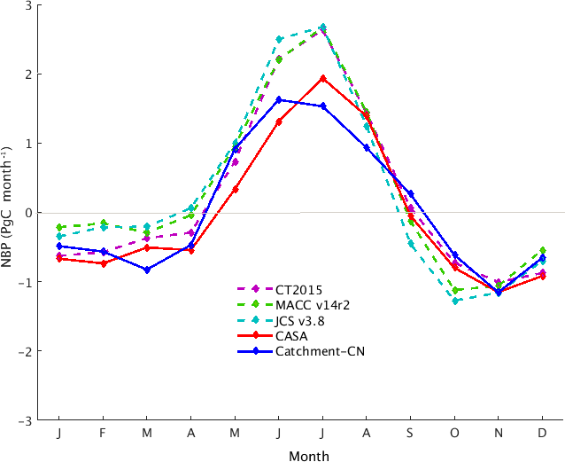
Figure 3 Monthly mean of terrestrial NBP of the Catchment-CN model (blue), of the CASA GFED3 model (red) and of three atmospheric inversions (dotted lines), for the period of 2004–2014. Positive (negative) NBP values indicate that land is a carbon sink (source).

3.2 Evaluation of simulated NBP against multiple datasets

The mean global net carbon fluxes from our control simulation were compared with the CASA GFED3 model estimates (which, in fact, serve as a prior to CarbonTracker; CarbonTracker Documentation CT2015 Release, 2016) as well as against the three aforementioned atmospheric inversion estimates (MACC v14r2, CarbonTracker 2015 and Jena CarboScope v3.8). In Fig. 3, the phase of the climatological NBP from the Catchment-CN model (solid blue) agrees well with that of the inversions (dotted curves). These datasets agree, for example, on the time during spring at which the land shifts from being a carbon source to a carbon sink. The CASA GFED3 model (solid red) shows a delay in the shift, a feature noted in previous studies (e.g., Ott et al., 2015).

The annual NBP from Catchment-CN (+0.53 Pg C year⁻¹) indicates that the land is a carbon sink, though the value is smaller than the mean of the sinks estimated by the three atmospheric inversions (+3.2 Pg C year⁻¹). The reason for the smaller value is unclear; we note only that the sink strength produced by the model reflects the net effect of a multitude of physical processes (underlying GPP, respirations and fire) in the model, processes that can interact with each other in complex ways.

The seasonal and zonal dependence of the Catchment-CN NBP is, in any case, within the spread of the inversions and the CASA GFED3 model (Fig. S2). The boreal summer (JJA) global carbon sink of Catchment-CN is approximately three-quarters of the inversion estimates (Fig. 3) and is relatively weak in the northern boreal ecosystem (Fig. S2c). This weaker summer global carbon sink is caused, in part, by the underestimated summer GPP (Fig. 2d) and perhaps also by the respiration values produced (Fig. S3). During December, January and February, the model NBP agrees with the inversions and the CASA GFED3 model estimates in the Northern Hemisphere, but it mostly follows the MACC v14r2 inversion in the Southern Hemisphere tropics where the inversions show disagreement in sign (Fig. S2a). The spring and fall NBP values from Catchment-CN lie within the range of the inversion estimates (MAM in Fig. S2b; SON in Fig. S2d).

3.3 Sensitivity of Catchment-CN fluxes to enrichment of CO₂

Our analysis in Sect. 3.4 will focus on how simulated GPP responds to various facets of the spatiotemporal character of the imposed atmospheric CO₂ forcing. It is thus particularly appropriate to evaluate the model's sensitivity to CO₂ variations.

The Large-Scale Free-air CO₂ Enrichment (FACE) experiments provide valuable data for such an evaluation. In these experiments, CO₂ is released into the air and advected by natural wind over the vegetation within experimental plots; the resulting CO₂ concentrations were increased by about 200 ppm above ambient conditions. Net primary productivity (NPP) observations over the FACE plots were compared to those over control plots with no CO₂ increase (e.g., Ainsworth and Long, 2004; Norby et al., 2005; Norby and Zak, 2011). Here we focus on two particular temperate forest FACE experiments: Duke FACE (35.58^∘ N, 79.5^∘ W) (Hendrey et al., 1999) and Oak Ridge National Laboratory (ORNL) FACE (35.54^∘ N, 84.20^∘ W) (Norby et al., 2001), well-documented field experiments that have been used in previous model–data comparison studies (e.g., Hickler et al., 2008; Piao et al., 2013; Zaehle et al., 2014; Walker et al., 2014).

To mimic these FACE experiments, we performed a supplemental numerical experiment with the Catchment-CN model (beyond the experiments outlined in Sect. 2.3): the control simulation was repeated but with the atmospheric CO₂ forcing increased artificially by 200 ppm. In this supplemental experiment, the CO₂ enrichment was applied globally starting on 1 January 2001, though we focus here on the simulated increases in NPP (relative to the control simulation, 3hCO2) within the land elements containing the Duke and ORNL FACE sites (i.e., the closest tile for each site). Because the original CLM4's NPP increase was found in a past study (with a similar experiment) to be low after the first year of the CO₂ enrichment, presumably due to an insufficient supply of mineralized nitrogen in the model for the plants' increased nitrogen demand associated with the CO₂-induced increase in the rate of photosynthesis (Zaehle et al., 2014), we evaluate here only the first year's simulation of NPP. Note that we started the CO₂ enrichment in 2001, whereas the actual FACE experiments began in earlier years (August 1996 for Duke and April 1998 for ORNL).

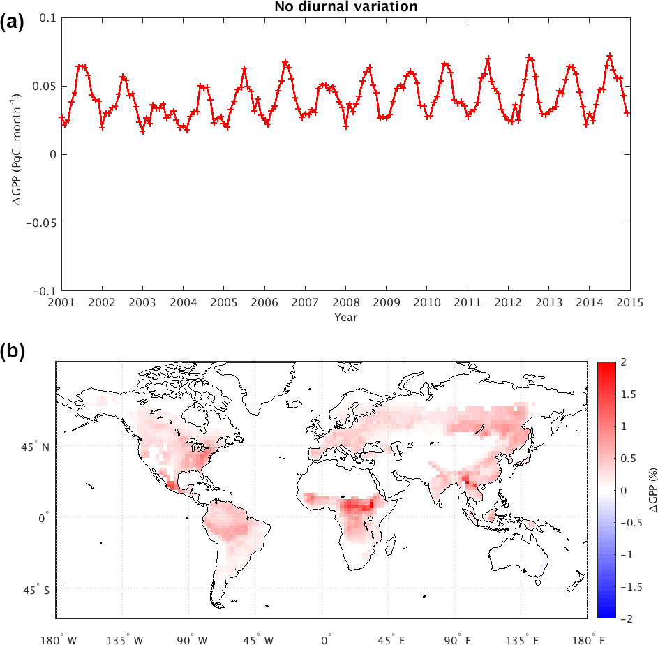
Figure 4 (a) Change in mean global GPP (Pg C month⁻¹) due to removal of diurnal variability in atmospheric CO₂ concentration (i.e., GPP from the dCO2 experiment minus that from the control). (b) Map of time-averaged GPP changes as a percentage (%). The tile-based model GPP values were aggregated to $\mathrm{2}{}^{\circ }\times \mathrm{2.5}{}^{\circ }$ for visualization purposes.

In this CO₂-enriched simulation, the Catchment-CN model produces an 18 % increase in NPP during the first year for the Duke site and a 15 % increase for the ORNL site. These results are at the low end of the observations for the Duke site (25±9 %) and underestimate the observed response at the ORNL site (25±1 %); the model does not capture the full sensitivity measured in the experiments. This underestimation must be kept in mind when interpreting our main results in the following section. For example, we forced our model with MERRA-2 meteorology instead of the site meteorology, and we applied the CO₂ stepwise increase in different years compared to the FACE experiment. In any case, our model results are still relevant to the interpretation and evaluation of the bottom-up estimates of GPP and NBP based on a dynamic global vegetation model (DGVM) found in the literature. For example, the average increase in NPP across the 11 DGVMs participating in a similar experiment was about 26 % (ranging from 9 % to 35 %) for the Duke site and 20 % (ranging from 7 % to 30 %) for the ORNL site (Zaehle et al., 2014; in their Fig. 5), somewhat similar to the increases found with our model. We can infer, then, that the sensitivities uncovered with our model experiments likely also apply to other models, including those providing global GPP and NBP estimates to the scientific community.

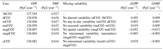
Table 1 Changes in mean global GPP and NBP for 2001–2014, resulting from a series of simulations representing the removal of temporal and spatial variability in atmospheric CO₂ concentrations. Delta (Δ) indicates the difference due to removal of spatial–temporal variability (see Fig. 1 for description).

3.4 Global-scale sensitivity of carbon fluxes to imposed CO₂ variability

Here we present the results of the experiments outlined in Fig. 1, with each facet of variability considered separately.

3.4.1 Diurnal variability in CO₂ (dCO2–3hCO2)

Figure 4 compares the results of dCO2 to those of the control simulation, thereby revealing the impact of the CO₂ diurnal cycle on simulated GPP and NBP. Figure 4a shows the time series of global mean GPP differences (dCO2 minus control) over the 14-year period; removing the diurnal variability clearly increases GPP, and the effect is particularly large in boreal summer (0.07 Pg C month⁻¹, equivalent to 0.8 Pg C year⁻¹). Figure 4b shows that most of the increases are in the tropics and in the far eastern areas of the Northern Hemisphere continents. Almost no region shows a decrease in GPP associated with the removal of the CO₂ diurnal cycle. As indicated in Table 1, removing the CO₂ diurnal cycle leads to an overall increase in global mean GPP of 0.497 Pg C year⁻¹ and a change in the global mean NBP of 0.100 Pg C year⁻¹.

The changes evident in Fig. 4 make sense in the context of the daily variations in atmospheric CO₂ noted in many studies (e.g., Denning et al., 1995, 1999). In nature (and as captured in the control simulation), the nighttime atmospheric CO₂ within the planetary boundary layer is higher than the daily mean value due to the shutdown of photosynthetic activity. Correspondingly, midday CO₂ concentrations are lower near the surface due to the plants' photosynthetic uptake of CO₂. In experiment dCO2, applying the daily mean CO₂ concentration at all hours of the day has the effect of imposing a higher CO₂ concentration during the daytime, when photosynthesis occurs, and this has the effect of artificially “fertilizing” the surface – the extra CO₂ imposed during the daytime makes photosynthesis more productive, increasing GPP. The GPP change in the tropics accounts for about two-thirds of the mean global GPP change, which is not surprising given the region's high productivity over the whole year.

3.4.2 Day-to-day variability in CO₂ (mCO2–dCO2)

The day-to-day variability in CO₂, as influenced, for example, by synoptic-scale weather and its impacts on atmospheric transport, is removed in experiment mCO2 relative to experiment dCO2. Table 1 indicates a negligible impact of this modification on the simulated global GPP and NBP compared to the impact of sub-daily CO₂ variations. The impacts on the temporal changes in the carbon fluxes and on the spatial distribution of the fluxes are similarly minimal (not shown).

Figure 5 (a) Change in mean global GPP (Pg C month⁻¹) due to removal of seasonal variability in atmospheric CO₂ concentration (i.e., GPP from the maCO2 experiment minus that from the mCO2 experiment). (b) Map of time-averaged GPP changes as a percentage (%).

3.4.3 Seasonal variability in CO₂ (maCO2–mCO2)

The maCO2 experiment forces the land surface with yearly averaged, but spatially varying, atmospheric CO₂. The resulting increases in GPP (maCO2 minus mCO2) in Fig. 5a thus reflect the impact of seasonal CO₂ variations. By applying the yearly averaged CO₂ concentration all year long, vegetation outside of the tropics experiences higher CO₂ concentrations during the spring and summer seasons, when photosynthesis is highest, than it would have otherwise; in nature photosynthetic drawdown of atmospheric CO₂ acts to reduce warm season CO₂ concentrations below the annual mean. The artificial warm season fertilization of the vegetation in the maCO2 case leads to an increase in growing season GPP (Fig. 5a).

A comparison of Figs. 4 and 5 shows that the influence of seasonal CO₂ variations is smaller than that of diurnal variations, which is consistent with the fact that the amplitude of the CO₂ seasonal cycle is about 10–20 ppm while that of the diurnal cycle is about 5 times larger (up to ∼120 ppm) in boreal summer (Fig. S4). The response of GPP to the seasonal variability in atmospheric CO₂ is highest in the Northern Hemisphere high latitudes (Fig. 5b), for which the distinction between cold season and warm season photosynthesis is largest. The regional- and seasonal-scale impact of this variability is further discussed in Sect. 3.5.

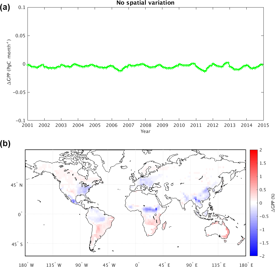
Figure 6 (a) Change in mean global GPP (Pg C month⁻¹) due to removal of spatial variability in atmospheric CO₂ concentration (i.e., GPP from the magCO2 experiment minus that from the maCO2 experiment). (b) Map of time-averaged GPP changes as a percentage (%).

3.4.4 Spatial variability in CO₂ (magCO2–maCO2)

Figure 6 shows the impact of applying in experiment magCO2 a globally uniform yearly averaged atmospheric CO₂ rather than a spatially varying distribution (e.g., with the inter-hemisphere gradient). In contrast to the above impacts of reducing temporal variability, the loss of spatial variability in atmospheric CO₂ leads to a global GPP decrease (Fig. 6a, showing results for magCO2 minus maCO2). This decrease in fact tends to partially offset the global GPP increases seen in the other experiments. Loss of spatial variability in CO₂ results in an overall reduction in global mean GPP of −0.052 Pg C year⁻¹ and a change in the global mean NBP of −0.012 Pg C year⁻¹ (Table 1).

Notably, the sign of the GPP change associated with the removal of CO₂ spatial variability is not globally uniform (Fig. 6b). In the absence of the large-scale inter-hemispheric gradient (Fig. S5), the GPP change is mostly negative in the densely vegetated areas of the Northern Hemisphere continents and positive in the Southern Hemisphere. GPP decreases are especially large in Europe, in the eastern US, in eastern China, and in tropical regions (e.g., the southeast Asia, Amazon and Congo rainforests), and these changes are only partially compensated for by GPP increases in extratropical Southern Hemisphere land areas such as the South American Atlantic forests and Cerrado. For densely vegetated areas, the pattern of the GPP change correlates well with changes in the imposed atmospheric CO₂ (Fig. S5); the agreement is less evident in areas with sparse vegetation.

Figure 7 (a) Change in mean global GPP (Pg C month⁻¹) due to removal of the trend in the interannual variability in atmospheric CO₂ concentration (i.e., GPP from the cCO2 experiment minus that from the magtCO2 experiment). (b) Map of time-averaged GPP changes in percent (%).

3.4.5 Interannual variability in CO₂ (magtCO2–magCO2 and cCO2–magtCO2)

Finally, in experiments magtCO2 and cCO2, the interannual variability in atmospheric CO₂ is removed in a stepwise manner. First, in magtCO2, year-to-year variations in CO₂ are removed while retaining the longer-term growth trend. This causes little change in global mean GPP and NBP (Table 1). The impacts on the temporal and spatial distribution of the fluxes are also negligible (not shown).

Conversely, when the observed long-term trend in atmospheric CO₂ is also removed (cCO2), increases in the global GPP are seen early in the simulation (2001–2008), and decreases are seen in the later part (2009–2014) (Fig. 7a, showing results for cCO2 minus magtCO2). In Fig. 7b, the removal of the long-term trend is seen to affect GPP mostly in the tropics, leading to an additional change in global mean GPP of 0.078 Pg C year⁻¹ (Table 1). While this time-mean change is smaller than that associated with neglecting diurnal variability, the differences at the beginning and end of the period (1.4 Pg C year⁻¹ between year 2001 and year 2014) are comparable to, or even larger than, the diurnal variability impact. These larger differences may have relevance to some period-specific model-based GPP estimates in the literature.

3.5 Regional- and seasonal-scale sensitivity of carbon fluxes to imposed CO₂ variability

The Atmospheric Tracer Transport Model Intercomparison Project (TransCom) 3 experiment (Gurney et al., 2000) defined a number of land and ocean source–sink regions of interest for the estimation of uncertainty in atmospheric inversion-based carbon flux estimates. The 11 terrestrial regional boundaries shown in their basis function map (http://transcom.project.asu.edu/transcom03_protocol_basisMap.php, last access: November 2017) offer a convenient framework for characterizing, in one place, the relative impacts of the different facets of spatiotemporal CO₂ variability on carbon fluxes and how the relative importance of these different facets varies across the globe. Such a characterization is presented here in the form of histograms (Fig. 8); together, the histograms succinctly capture our regional and seasonal findings.

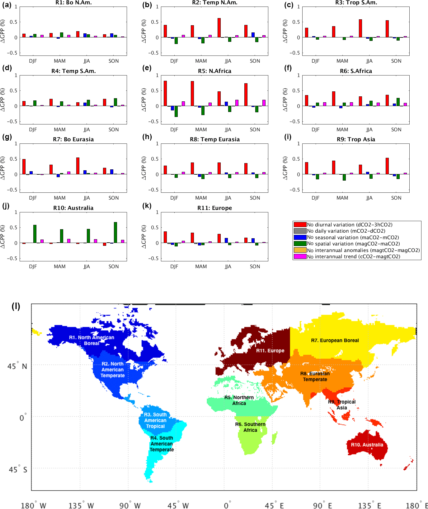
Figure 8 Regional- and seasonal-scale impacts of spatiotemporal CO₂ variabilities on GPP. Incremental change in GPP associated with each added facet of CO₂ variability is shown as a percentage of the previous experiment's regional GPP. The map in (l) shows the regional boundaries of TransCom land regions (reconstructed from the basis function map in http://transcom.project.asu.edu/transcom03_protocol_basisMap.php, last access: November 2017).

Figure 8 shows, for example, that ignoring the diurnal variation in atmospheric CO₂ results in the overestimation of GPP in all seasons and in all TransCom regions except for Australia, where it slightly reduces GPP and where the influence of the spatial CO₂ variability is dominant. Spatial CO₂ variability is also found to partially compensate for diurnal variability in the Northern Hemisphere temperate regions (North America and Eurasia; see Fig. 8b and h) and in North Africa (Fig. 8e).

Seasonal CO₂ variations are found to be particularly important in Northern Hemisphere high-latitude regions; during fall, the GPP change induced by seasonal CO₂ variations is comparable to (and in the same direction as) that caused by diurnal variations (Fig. 8a and g). Similarly, seasonal variations have an important impact on GPP in Europe during fall (i.e., SON in Fig. 8k), presumably due to the presence of mixed (boreal and temperate) forests there; this impact is large enough to offset the fall GPP reduction induced by ignoring spatial CO₂ variations (Fig. 8b and k). Day-to-day and year-to-year variations in atmospheric CO₂ have little impact anywhere, reaffirming our global-scale analysis. The long-term trend in CO₂, however, has a relatively large percentage impact in the two African regions (Fig. 8e and f) – ignoring this trend in CO₂ in these regions leads to increased GPP. While diurnal CO₂ variations are important for all seasons across nearly all regions, the interplay among seasonal variations, spatial variations and long-term trends appears to be crucial to certain seasonal and/or regional GPP estimations.

4 Discussion

Overall, our results indicate that ignoring temporal variability in atmospheric CO₂ in the bottom-up estimation of carbon fluxes with a representative offline model can lead to overestimates of global GPP of up to 0.5 Pg C year⁻¹ (see Table 1). The corresponding estimates of the strength of the land carbon sink may be too high by about 0.1 Pg C year⁻¹. The most important facets of temporal CO₂ variability are found to be diurnal variability and the trend in interannual variability; ignoring them contributes 0.5 and 0.08 Pg C year⁻¹, respectively, to the global GPP overestimate. Conversely, ignoring spatial variability in atmospheric CO₂ reduces the mean global GPP by 0.05 Pg C year⁻¹ (Table 1); that is, ignoring this spatial variability contributes to an underestimation of global GPP.

Liu et al. (2016) performed, in essence, a subset of the experiments examined here. In agreement with our findings, they show that the seasonal variation in CO₂ lowers global GPP and that the spatial variation in CO₂ increases it. The authors in fact suggest that ignoring spatial variability in CO₂ largely compensates for ignoring the temporal variability, though they admit that the use of marine background CO₂ concentrations in their baseline simulation, which are lower than the surface-layer CO₂ values seen by plants, may have exaggerated the spatial-variability-related GPP reduction. Our more comprehensive set of experiments allows us to examine, in addition, the effects of diurnal and interannual CO₂ variability on global carbon fluxes, which turn out to be more important than the effects of either seasonal or spatial CO₂ variability. Note that the neglect of diurnal variability may partially explain the overestimate (relative to observation-based datasets) noted in the literature regarding tropical GPP simulated by CLM4 (Bonan et al., 2011). Also note that because the Catchment-CN model underestimates the response to CO₂ fertilization seen in the FACE experiments, the impact of diurnal variability at work in nature could be somewhat larger than our estimate here.

Table 2 Differences in mean global GPP and NBP compared to the case that uses the most popular atmospheric CO₂ forcing (magCO2). The values are the global mean of 2001–2014.

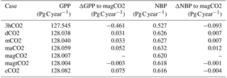
Again, the overestimation of the global carbon sink associated with ignoring the temporal variability in atmospheric CO₂ is 0.1 Pg C year⁻¹ (Table 1). This, again, is a small deviation relative to estimates of the overall land sink; Le Quéré et al. (2016, their Fig. 2), for example, cite an estimate of 3.1 Pg C year⁻¹ for this sink. This small sensitivity has relevance to the ongoing CMIP6 project. Through our experiments we quantify in effect the expected impacts of the minimum requirement recommended by CMIP6 for historical simulations (Eyring et al., 2016), namely, that of globally uniform annual mean CO₂ with interannual variations and of the CMIP6 option of including latitudinal and seasonal variations (Meinshausen et al., 2017). The small sensitivities we uncover suggest that these recommendations, while not harmful, will nevertheless have little impact on the global-scale fluxes produced in CMIP6. Note again that the first approach, that of using globally uniform annual mean CO₂ with interannual variations, was effectively used in our magCO2 experiment; as shown in Table 2 and Fig. S6a, the global mean fluxes produced in our other experiments are indeed similar to those produced in magCO2. The land modeling and carbon cycle community need not have been too concerned over the years about the global impacts of CO₂ variability finer than what has commonly been applied in past studies (i.e., annually increasing transient CO₂).

This, however, may be an overstatement. It is worth noting that the bias of 0.1 Pg C year⁻¹ associated with spatiotemporal CO₂ variability is in fact a significant fraction of the uncertainty in this value (listed by Le Quéré et al. (2016) as ±0.9 Pg C year⁻¹). Also, various model intercomparison studies, e.g., CMIP6, TRENDY and MsTMIP, may need to consider the full range of spatiotemporal CO₂ variability when estimating terrestrial productivity and net sink size on regional and seasonal scales (Fig. 8), for which the impacts can be larger. The growing-season NBP bias can be as large as −6 % from our analysis (MAM in Fig. S7b), and the local impact well exceeds the global impact (Fig. S6b). It is thus sensible to impose, if at all possible, realistic CO₂ variability in carbon budget analyses.

Our results have some broader implications. They suggest that the diurnal rectifier effect, the substantial CO₂ covariations that are introduced with daily variations in photosynthesis and boundary layer turbulence, in a DGVM-based NBP may need to be considered in future atmospheric inversion studies that use it as a prior, given that biases in the prior can propagate into errors in the inversion products. Furthermore, they suggest that if the land carbon component of an Earth modeling system is not coupled to its atmospheric component with a sub-daily time step (e.g., in a climate change study), the bias can be carried into the evolution of regional and seasonal land carbon dynamics, albeit the global effect may be minor. Finally, our results indicate a negligible impact of spatiotemporal CO₂ variability on water cycle variations through their impacts on stomatal conductance and thus evapotranspiration (not shown). The interaction between the water and carbon cycles in this study is thus limited; more careful analysis in a fully coupled modeling system, however, may reveal some interesting connections.

5 Conclusions

In summary, the key results from this study are as follows.

1. The carbon flux estimates of the Catchment-CN model generally agree with other statistics-based and model-based estimates. The GPP estimates from our control simulation (which utilized the full complement of atmospheric CO₂ variability contained within the CarbonTracker dataset) validate reasonably well with the MTE-GPP dataset, a widely used product for model evaluation, and our NBP estimates are also consistent to the first order with results from the diagnostic CASA GFED3 model (a bottom-up approach) and the atmospheric inversions (a top-down approach). The agreement supports our use of the Catchment-CN model in the experiments outlined in Fig. 1.

2. Ignoring the various facets of temporal variability in CO₂ leads to increases in the mean global GPP simulated by the process-based model. The diurnal component of the variability is particularly important; ignoring it increases the estimated mean global GPP by 0.5 Pg C year⁻¹.

3. Ignoring the spatial variability in atmospheric CO₂, however, leads to a decrease in mean global GPP, with decreases in the Northern Hemisphere and increases in the Southern Hemisphere. The overall decrease of 0.05 Pg C year⁻¹ is smaller than the increase associated with ignoring temporal variability.

4. For estimating multiyear mean GPP, the effect of neglecting interannual variations in atmospheric CO₂ is small. Ignoring the long-term trend, however, can have important implications; the differences at the beginning and end of the period (up to a 1.4 Pg C year⁻¹ difference between the year 2001 and the year 2014 in this study) can be much greater than the effect of ignoring the diurnal CO₂ variation.

5. The impacts of ignoring temporal and spatial variability vary with region. The sensitivity in the tropics tends to be the largest. The seasonal variability in atmospheric CO₂ plays a particularly important role in the NH boreal regions during fall. Spatial variability in CO₂ is important in temperate regions, offsetting the local impacts of temporal variability on GPP.

6. The magnitude of the sensitivities found is small, particularly at the global scale. The proper imposition of realistic CO₂ variability in offline studies will incur only slight modifications to the terrestrial carbon fluxes computed. This said, the imposition of realistic CO₂ variability is straightforward and could have more significant impacts on quantified regional and seasonal fluxes.

The carbon flux estimation sensitivities highlighted herein are, of course, model dependent. The sensitivities are subject to model-specific assumptions and parameters (see the MsTMIP inter-model comparison study; Ito et al., 2016) and to the selection of the meteorological inputs (Poulter et al., 2011). Still, as noted in Sect. 3.3, the sensitivity of GPP to CO₂ increases in the Catchment-CN model is similar to that in other state-of-the-art models, suggesting that the results herein are broadly applicable and that DGVM-based estimates in the literature of global GPP may be subject to the noted biases, small as they are found to be here.