the Creative Commons Attribution 4.0 License.
the Creative Commons Attribution 4.0 License.
 | 09 Nov 2018
Reviews and syntheses: the GESAMP atmospheric iron deposition model intercomparison study
Maria Kanakidou
Athanasios Nenes
Maarten C. Krol
Natalie M. Mahowald
Rachel A. Scanza
Douglas S. Hamilton
Matthew S. Johnson
Nicholas Meskhidze
Jasper F. Kok
Cecile Guieu
Alex R. Baker
Timothy D. Jickells
Manmohan M. Sarin
Srinivas Bikkina
Rachel Shelley
Andrew Bowie
Morgane M. G. Perron
Robert A. Duce
This work reports on the current status of the global modeling of iron (Fe) deposition fluxes and atmospheric concentrations and the analyses of the differences between models, as well as between models and observations. A total of four global 3-D chemistry transport (CTMs) and general circulation (GCMs) models participated in this intercomparison, in the framework of the United Nations Joint Group of Experts on the Scientific Aspects of Marine Environmental Protection (GESAMP) Working Group 38, “The Atmospheric Input of Chemicals to the Ocean”. The global total Fe (TFe) emission strength in the models is equal to ∼72 Tg Fe yr−1 (38–134 Tg Fe yr−1) from mineral dust sources and around 2.1 Tg Fe yr−1 (1.8–2.7 Tg Fe yr−1) from combustion processes (the sum of anthropogenic combustion/biomass burning and wildfires). The mean global labile Fe (LFe) source strength in the models, considering both the primary emissions and the atmospheric processing, is calculated to be 0.7 (±0.3) Tg Fe yr−1, accounting for both mineral dust and combustion aerosols. The mean global deposition fluxes into the global ocean are estimated to be in the range of 10–30 and 0.2–0.4 Tg Fe yr−1 for TFe and LFe, respectively, which roughly corresponds to a respective 15 and 0.3 Tg Fe yr−1 for the multi-model ensemble model mean.
The model intercomparison analysis indicates that the representation of the atmospheric Fe cycle varies among models, in terms of both the magnitude of natural and combustion Fe emissions as well as the complexity of atmospheric processing parameterizations of Fe-containing aerosols. The model comparison with aerosol Fe observations over oceanic regions indicates that most models overestimate surface level TFe mass concentrations near dust source regions and tend to underestimate the low concentrations observed in remote ocean regions. All models are able to simulate the tendency of higher Fe concentrations near and downwind from the dust source regions, with the mean normalized bias for the Northern Hemisphere (∼14), larger than that of the Southern Hemisphere (∼2.4) for the ensemble model mean. This model intercomparison and model–observation comparison study reveals two critical issues in LFe simulations that require further exploration: (1) the Fe-containing aerosol size distribution and (2) the relative contribution of dust and combustion sources of Fe to labile Fe in atmospheric aerosols over the remote oceanic regions.
- Article
(6184 KB) - Full-text XML
-
Supplement
(8341 KB) - BibTeX
- EndNote


Oceans are important for the Earth system's functioning, currently absorbing roughly 27 % of total CO2 emissions (e.g., Le Quéré et al., 2013), providing about half of atmospheric oxygen and being a source of biomass that helps sustain life on our planet. Iron (Fe) is a key element for marine life (Duce and Tindale, 1991; Fung et al., 2000) and is required for photosynthesis and respiration. As an essential micronutrient, Fe (co-)limits ocean productivity over large regions (Boyd et al., 2005; Jickells et al., 2005; Martin et al., 1991; Moore et al., 2013), influences the nitrogen fixation capability of diazotrophs in oligotrophic regions (Falkowski, 1997; Falkowski et al., 2000) and generally affects the transport and sequestration of carbon into the deep ocean (Maher et al., 2010). Atmospheric deposition is considered to be an important external Fe source for the open ocean (Jickells et al., 2005; Tagliabue et al., 2017). Micronutrient Fe delivered via atmospheric pathways may influence the primary and export production of carbon over the high-nutrient low-chlorophyll (HNLC) oceanic regions (i.e., the oceanic regions where Fe is the limiting factor for phytoplankton productivity). However, significant Fe inputs from continental margins and hydrothermal vents are also supplied to the global ocean, regulating the ocean biogeochemical cycles. Moreover, riverine Fe inputs are currently estimated to be 1–2 orders of magnitude smaller that the atmospheric pathway (e.g., Tagliabue et al., 2016), affecting mainly coastal regions, while icebergs and glaciers could also be important for the polar oceans (Raiswell et al., 2016).
An understanding of the impact of Fe on global marine productivity requires a knowledge of the rates and locations of Fe supply to the ocean, and of the physicochemical forms of Fe that can be utilized by marine biota (i.e., those that are bioavailable). The bioavailability of Fe is a complex issue (e.g., Lis et al., 2015; Morel et al., 2008) and several naming conventions and abbreviations have been used to characterize the atmospheric supply of potentially bioavailable Fe to the global ocean (Baker and Croot, 2010; Shi et al., 2012). It has been widely assumed that soluble Fe can be considered, as a first approximation, to be bioavailable (Baker et al., 2006a, b). Therefore, a common experimental practice to determine the bioavailable Fe fraction in Fe-containing aerosols is the quantification of Fe in a leachate solution that passes through a 0.45, 0.2 or 0.02 µm sized filter (see Meskhidze et al., 2016, and references therein). However, due to its operational definition, it has been shown that this filterable Fe may contain both soluble and colloidal forms of Fe (Jickells and Spokes, 2001; Raiswell and Canfield, 2012). Upon deposition to the surface ocean, the soluble form of Fe delivered through atmospheric pathways can either enter the dissolved Fe pool or precipitate out as large (oxy)hydroxide particles (de Baar and de Jong, 2001; Boyd and Ellwood, 2010; Meskhidze et al., 2017; Turner and Hunter, 2001). Consequently, the impact of atmospheric Fe on marine biogeochemistry depends on both the total Fe (TFe) deposition and its solubility, keeping in mind that the bioavailable fraction of Fe in seawater will also then change due to post-atmospheric deposition ocean processes (e.g., Baker and Croot, 2010; Chen and Siefert, 2004; Meskhidze et al., 2017; Rich and Morel, 1990).
On the global scale mineral dust is the dominant source of Fe to the atmosphere (∼95 %; Mahowald et al., 2009). The average Fe content in upper crustal minerals is 3.5 % (e.g., Duce and Tindale, 1991), but this can vary considerably, depending on the underlying mineralogy (and geography) of the dust source (Journet et al., 2014; Nickovic et al., 2012, 2013). According to Journet et al. (2014), the Fe content of various minerals is as follows: hematite (69.9 %), goethite (62.8 %), chlorite (12.3 %), vermiculite (6.71 %), illite (4.3 %), smectite (2.6 %), feldspars (0.34 %) and kaolinite (0.23 %) in clay- and silt-sized soil particles (i.e., soil particles with diameters <2 and 2–50 µm, respectively). Fe-containing aerosols also originate from wildfires and biomass burning (Guieu et al., 2005; Mahowald et al., 2005; Oakes et al., 2012; Paris et al., 2010) and anthropogenic combustion processes, such as coal and oil fly ash (Luo et al., 2008), including ship oil combustion (Ito, 2013). Other sources of Fe oxides can be also identified in the atmosphere, which are attributed to volcanic eruptions (Benitez-Nelson et al., 2003; Langmann et al., 2010) and to a lesser extent meteors (Johnson, 2001).
The use of global biogeochemical numerical models and surface observations is an excellent way to better understand the past, present and future atmospheric supply to the oceans, as well as to quantify the resultant effect on the ocean biological productivity and the carbon uptake. Modeling of the atmospheric supply of soluble Fe to the global ocean is challenging, due to the multitude and complexity of the forms under which Fe can be present in aerosol emitted to the atmosphere (Meskhidze et al., 2017), as well as the variety and complexity of processes which alter the solubility of Fe during its transport through the atmosphere (Baker and Croot, 2010). Indeed, the soluble fraction of Fe in atmospheric aerosols may include different Fe forms in the ferric oxidation state (Fe(III)) (Fu et al., 2012), ferrihydrite and amorphous precipitates, Fe-oxide nanoparticles (Shi et al., 2009), Fe-organic complexes (Cheize et al., 2012) and Fe in the ferrous oxidation state (Fe(II)) (Raiswell and Canfield, 2012). The atmospheric modeling community is mostly focused on the soluble fraction of the deposited Fe over the oceans and for this work the general term labile Fe (LFe) is used to represent the overall soluble Fe in simulated atmospheric aerosol. Both the TFe and LFe atmospheric deposition can be used in ocean biogeochemical modeling. For example, total Fe is used for the comparison of particulate Fe with the measurements in ocean biogeochemistry models (e.g., Ye and Völker, 2017), while LFe can be assumed to be readily available to the marine ecosystem. Note that the less labile fraction of TFe can be slowly dissolved from particulate Fe in the ocean during the sinking of mineral particles (e.g., roughly 0.01 % per day; Bonnet, 2004); however, the dissolution of Fe is species dependant and affected by spatiotemporal variations in the ocean.
During recent decades, intensive research has been carried out to elucidate the origin, nature and magnitude of LFe fluxes to the surface ocean. Soils may include a small fraction of LFe – roughly 0.1 % (e.g., Ito and Shi, 2016) – considered as impurities attached to minerals such as illite, smectite, kaolinite and feldspars (e.g., Ito and Xu, 2014). Fe-containing fly ash has been observed to be present as ferric sulfate salts or nanoparticulate Fe and is highly soluble (Fu et al., 2012; Schroth et al., 2009), as it is mainly formed via high-temperature combustion followed by sulfuric acid condensation (Sippula et al., 2009). However, the form and the chemical properties of Fe in emissions can vary substantially for each combustion source (Ito, 2013; Wang et al., 2015), with the initial soluble fraction in combustion emissions estimated to be about 77 %–81 % in oil fly ash (Schroth et al., 2009), 20 %–25 % in coal fly ash (Chen et al., 2012) and 18 %–46 % in biomass fly ash (Bowie et al., 2009; Oakes et al., 2012). Recently, Matsui et al. (2018) suggested, based on observed magnetite concentrations, that emissions of anthropogenic combustion Fe in global models could be significantly underestimated, and that the atmospheric burden of Fe is potentially up to 8 times greater than previous estimates have suggested (Luo et al., 2008). LFe can be also formed in the atmosphere during the atmospheric processing of mineral dust and combustion aerosols (Ito, 2012; Ito and Feng, 2010; Johnson and Meskhidze, 2013; Meskhidze et al., 2005; Myriokefalitakis et al., 2015). We use the general term “solubilization” here to describe the process that converts Fe from relatively insoluble minerals to soluble Fe during atmospheric transport and photochemical transformation in the aqueous solution of aerosols and clouds.
Iron solubility (i.e., the fraction of total Fe that is soluble) in atmospheric aerosols over the Atlantic and Pacific oceans has been observed to be in the range of 0.1 %–67 % during oceanographic cruises (Baker et al., 2006a; Furutani et al., 2010), with even higher solubilities (up to 80 %) measured in precipitation samples in the Southern Ocean (Heimburger et al., 2013). During atmospheric transport, coating of Fe-containing dust particles by acidic compounds (e.g., sulfates and nitrates) increases the Fe solubility. When this process is taken into account in model simulations (e.g., Meskhidze et al., 2005) it aids in explaining the observations. Indeed, measurements of fresh dust particles present low (≪1 %) initial solubilities (Chuang et al., 2005; Fung et al., 2000; Hand et al., 2004; Sedwick et al., 2007), while high aerosol solubilities are commonly observed at lower dust concentrations far from sources (Baker and Jickells, 2006; Sholkovitz et al., 2012; Oakes et al., 2012). Atmospheric processing of dust (Kumar et al., 2010; Meskhidze et al., 2003; Srinivas et al., 2014) is considered to be the best candidate for explaining these observations. These processes may also alter the global pattern of LFe deposition (Fan et al., 2004), especially within remote regions, such as the Atlantic, the Pacific (e.g., Sedwick et al., 2007) and the Southern Ocean (Ito and Kok, 2017; Johnson et al., 2010, 2011).
There is clear experimental evidence that atmospheric acidity – which is mainly driven by air pollution over highly populated regions especially over the Northern Hemisphere (e.g., Seinfeld and Pandis, 2006) as well as natural sources such as volcanic sulfur emissions and the oceanic emissions of dimethylsulfide (DMS) in relatively pristine ecosystems (e.g., Benitez-Nelson et al., 2003) – increases the dust solubility. Laboratory studies indicate that Fe solubilization from minerals under acidic conditions in aerosol or rain droplets (Brandt et al., 2003; Shi et al., 2011; Spokes et al., 1994) occurs on different timescales: from hours to weeks depending on the size and the type of the Fe-containing minerals (Shi et al., 2011), with amorphous and ultrafine Fe solubilized much faster in acidic solutions (Brandt et al., 2003) compared to the aluminosilicates (roughly 10–14 days). Other laboratory studies also support the occurrence of photoinduced reductive Fe solubilization under acidic conditions (e.g., Fu et al., 2010), a mechanism that involves electron transfer to Fe(III) atoms on the particle surface to produce Fe(II) (Larsen and Postma, 2001). The reductive solubilization of minerals that are rich in Fe is also observed to be accelerated in the presence of Fe(II) or Fe(II)-ligand complexes (Litter et al., 1994). The oxalate-promoted solubilization (e.g., Paris et al., 2011) is controlled by the breaking of Fe–O bonds at the mineral's surface due to the formation of a mononuclear bidentate ligand containing surface Fe (Yoon et al., 2004), with the solubilization rate significantly increased as the pH decreases. Luo et al. (2010) further prescribed pH and oxalate/hematite ratio dependent solubilization rates for mineral dust, based on the laboratory experiments of Xu and Gao (2008). For weakly acidic conditions (pH of 4.7) and various oxalate concentrations, a positive linear correlation between oxalate concentrations and the released LFe from different minerals has also been observed (Paris et al., 2011; Paris and Desboeufs, 2013). Laboratory investigations (Chen and Grassian, 2013; Siffert and Sulzberger, 1991) have indicated that even under highly acidic solutions (pH of 2–3), oxalic acid can be more important for the Fe solubilization process of dust and combustion aerosols than sulfuric acid through the formation of Fe(III)–oxalate complexes. Thus, the minerals' solubilization mainly depends on the proton concentration, the mineral surface concentration of organic ligands (such as oxalate), the sunlight and the ambient temperature (e.g., Hamer et al., 2003; Lanzl et al., 2012; Lasaga et al., 1994; Zhu et al., 1993).
The first modeling efforts that took the mixing of mineral dust with such anthropogenic acidic trace gases like sulfur dioxide (SO2) into account (Fan et al., 2004; Meskhidze et al. 2003, 2005; Solmon et al., 2009) showed considerable enhancements of atmospheric soluble Fe concentrations. A review by Mahowald et al. (2009) pointed out that human activity may have significantly modified the soluble Fe oceanic deposition flux, because anthropogenic combustion processes increased both Fe emissions and the acidity of atmospheric aerosols. Furthermore, recent studies (Meskhidze et al., 2017; Tagliabue et al., 2017) have also shown that atmospheric and oceanic organic ligands may increase the Fe solubilization in the atmosphere and in the ocean, by forming Fe complexes that further increase Fe bioavailability for the marine ecosystems. State-of-the-art global models clearly indicate a strong spatial and temporal variability of the atmospheric LFe supply to the global ocean, which can be partly attributed to atmospheric processing. The global LFe deposition flux is currently estimated to be in the range of 0.4–1.1 Tg Fe yr−1 (Ito and Kok, 2017; Ito and Shi, 2016; Ito and Xu, 2014; Johnson and Meskhidze, 2013; Luo et al., 2008; Myriokefalitakis et al., 2015; Wang et al., 2015).
In order to constrain a global picture of the influence of the present atmospheric composition on the Fe supply to the oceans, we perform a systematic comparison between models and between models and observations. We identify possible similarities and differences among models and between models and observations. The goals of the present study are to (1) quantify the magnitude of the atmospheric TFe and LFe fluxes to the global ocean as calculated by four state-of-the-art global atmospheric aerosol models, (2) explain the differences in the simulated LFe among the participating models, and (3) to provide multi-model ensemble TFe and LFe atmospheric Fe deposition fluxes for the next generation of ocean biogeochemistry modeling studies. Overall, the importance of this work lies in an extended review and synthesis of the current knowledge of global atmospheric Fe deposition fluxes in the ocean, aiming to provide ensemble model data to the scientific community, which will be able to be used in ocean biogeochemistry models and as comparative measures for atmospheric models.
The following discussion is organized into four sections. Section 2 describes the participating models and the observations used in this study. This section aims to build a concise view of the present-day understanding on the magnitude and the distribution of the TFe and LFe simulated deposition fluxes to the global ocean; ensemble model calculations are also presented. Section 3 presents and discusses the simulated global Fe atmospheric budgets and distributions. In Sect. 4, the uncertainties in the calculated surface aerosol Fe concentrations and deposition fluxes are discussed and the potential model biases are analyzed by attributing them to their major contributors. Finally, in Sect. 5 the findings of the present study are summarized, and recommendations for future research directions are put forward.
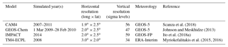
Table 1General description of the participating models used for the atmospheric Fe simulations. For multiple year simulations, the average was used.
2.1 Description of models
The global models participating in this study differ with respect to their spatial horizontal and vertical resolution, the meteorology, the emissions used for gas and aerosol species, and the aerosol microphysics (i.e., size distribution and refractive properties). They also differ in the gas- and aqueous- phase chemical schemes and the parameterizations of atmospheric transport and deposition processes. The main characteristics of the participating models are summarized in Table 1. Note, however, that for this intercomparison no requirements regarding specific year, meteorological conditions or emission inventories were set for the model simulations. Therefore, the data presented are mainly based on earlier published (or soon to be published) modeling experiments, which are evaluated and systematically analyzed here.
-
The Community Atmosphere Model version 4 (CAM4) is embedded within the National Center for Atmospheric Research (NCAR) Community Earth System Model version 1.0.5 (CESM 1.0.5; Hurrell et al., 2013). The CAM4 simulations are conducted with a horizontal resolution of (longitude×latitude) and 56 vertical layers up to 2 hPa; it is forced by NASA's Goddard Earth Observing System (GEOS-5) meteorology. The emission data sets for anthropogenic activities, such as fossil fuel and biofuel combustion, are taken from the Aerosol Comparison between Observations and Models (AeroCom) database (Dentener et al., 2006). Desert dust is modeled following the Dust Entrainment and Deposition (DEAD) module (Zender et al., 2003) with updates of the size fractions (Kok, 2011) and optics as described in Albani et al. (2014). The bin widths are prescribed at diameters of 0.1–1.0, 1.0–2.5, 2.5–5.0 and 5.0–10.0 µm and have fixed lognormal sub-bin distributions. Dust in CAM4 is speciated into six minerals, clays (illite, kaolinite and montmorillonite), feldspar, calcite and hematite (Scanza et al., 2015), with a total dust source of about 1767 Tg yr−1 calculated for the present day. Further details on the CAM4 model used for this work are provided in Scanza et al. (2018) and references therein.
-
The GEOS-Chem model is driven by assimilated meteorological fields from the Goddard Earth Observing System (GEOS-5) of the NASA Global Modeling Assimilation at a horizontal (latitude×longitude) grid resolution and 47 vertical levels up to 0.01 hPa. GEOS-Chem simulates the emissions and chemical transformation of sulfur compounds, carbonaceous aerosols and sea salt, and includes H2SO4–HNO3–NH3 aerosol thermodynamics solved by the ISORROPIA II thermodynamic model (Fountoukis and Nenes, 2007) coupled to an O3–NOx–hydrocarbon–aerosol chemical mechanism. GEOS-Chem combines the DEAD scheme with the source function used in the Goddard Chemistry Aerosol Radiation and Transport (GOCART) model. Once mineral dust is mobilized from the surface, the model uses four standard dust bins with diameter boundaries of 0.2–2.0, 2.0–3.6, 3.6–6.0 and 6.0–12.0 µm to simulate global dust transport and deposition, emitting 1614 Tg yr−1 of mineral dust globally. Further details regarding the GEOS-Chem model used for the this work can be found in Johnson and Meskhidze (2013) and references therein.
-
The Integrated Massively Parallel Atmospheric Chemical Transport (IMPACT) model (Rotman et al., 2004) is also driven by assimilated meteorological fields from the Goddard Earth Observation System – Forward Processing (GEOS–FP) of the NASA Global Modeling and Assimilation Office (Lucchesi, 2017) with a horizontal resolution of and 59 vertical layers up to 0.01 hPa. The model simulates the emissions, chemistry, transport and deposition of major aerosol species (Liu et al., 2005) and their precursor gases (Ito et al., 2007). IMPACT takes emissions of primary aerosols and precursor gases of secondary aerosols such as sulfate, nitrate, ammonium and oxalate into account. The emission data sets for anthropogenic activities such as fossil fuel use and biofuel combustion are taken from the Community Emission Data System (CEDS) (Hoesly et al., 2018). Fe-containing combustion and dust aerosols are distributed among four bins in the model, with diameters of <1.26, 1.26–2.5, 2.5–5 and 5–20 µm, respectively (Ito, 2015; Ito and Feng, 2010). The present-day emission estimates for natural sources as well as combustion aerosols from biomass burning are used together with anthropogenic emissions (Dentener et al., 2006; Ito et al., 2018a). A total dust source of 5070 Tg yr−1 is dynamically calculated by a physically based dust emission scheme (Kok et al., 2014a, b) in the model for the present day (Experiments 3 in Ito and Kok, 2017). The chemical composition of mineral dust and combustion aerosols can change dynamically from that in the originally emitted aerosols due to reactions with gaseous species. Aerosol pH is calculated from the internal particle composition (H+ and H2O) for each size bin by the thermodynamic equilibrium module (Jacobson, 1999). The aerosol acidity depends on the aerosol types, mineralogy, particle size, meteorological conditions and transport pathway of aerosols (Ito and Feng, 2010; Ito and Xu, 2014; Ito, 2015). A more detailed description of the IMPACT model used for this work can be found in Ito (2015), Ito and Kok (2017), Ito and Shi (2016) and references therein.
-
The TM4-ECPL global chemistry transport model simulates the oxidant (O3/NOx/HOx/CH4/CO) chemistry, accounting for non-methane volatile organic compounds, including isoprene, terpenes and aromatics, multiphase chemistry in clouds and aerosol water, as well as all major primary and secondary aerosol components, including sulfate, nitrate and secondary organic aerosols. TM4-ECPL is coupled with the ISORROPIA II thermodynamic model (Fountoukis and Nenes, 2007) and it uses modal size (lognormal) distributions to describe the evolution of fine and coarse aerosols in the atmosphere. Dust emissions, for the present version of the model, are calculated online based on the dust source parameterization of Tegen et al. (2002), as described in Myriokefalitakis et al. (2016); these updated dust source calculations should produce slightly higher (∼7 %) dust emissions of around 1181 Tg yr−1 compared to the modified AeroCom inventory (Dentener et al., 2006) that was taken into account in the previous version of the model (Myriokefalitakis et al., 2015). Dust is emitted in the fine and coarse mode with mass median radii (lognormal standard deviation) of 0.34 µm (1.59) and 1.75 µm (2.00), respectively. Furthermore, in the updated version of the model, the mineral-containing combustion aerosols are emitted with a number mode radius (lognormal standard deviation) of 0.04 µm (1.8) and 0.5 µm (2.0) for the fine and coarse modes, respectively (Dentener et al., 2006; Myriokefalitakis et al., 2016). All aerosol species in the model are subject to hygroscopic growth and removal processes that generally affect the mass median radius. The aerosol hygroscopic growth in the model is treated as a function of ambient relative humidity and the composition of soluble aerosol components and the uptake of water on aerosols change the particle size. The TM4-ECPL model is driven by the ECMWF (European Center for Medium-Range Weather Forecasts) Interim reanalysis project (ERA-Interim) meteorology and has a horizontal resolution of (latitude×longitude), 34 hybrid layers from the surface up to 0.1 hPa and a model time step of 30 min. Further details on the TM4-ECPL model used for this study can be found in Myriokefalitakis et al. (2015, 2016) and references therein.
2.1.1 Iron emission parameterizations
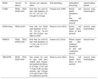
The primary Fe sources taken into account by the models can be roughly grouped as (1) mineral dust and (2) combustion sources. Various parameterizations or simplifications of the Fe emissions are adopted by the models, with the most important in the context of this paper being the Fe content and initial Fe solubility in emissions. The mean Fe content in dust emissions, as well as the initial Fe solubility in emissions taken into account by the participating models, are presented in the Supplement (Figs. S1 and S2, respectively). More detail is also given in the following:
-
Mineral dust emissions: Mineral-Fe primary sources are derived from the total mineral dust emissions, the fraction of specific Fe-containing minerals in dust emissions and the Fe content of each mineral (Table S1 in the Supplement). CAM4 uses a soil mineralogy map and the Fe content in soils is estimated based on mineralogical content (Claquin et al., 1999; Scanza et al., 2015, 2018; Zhang et al., 2015). GEOS-Chem and TM4-ECPL take the global soil mineralogy data set developed by Nickovic et al. (2012) into account. GEOS-Chem prescribes an initial Fe solubility of 0.45 % for the most reactive and poorly crystalline pool of Fe in desert top soils (Fig. S1), based on the synthesis of data from the Saharan and Sahel regions of northern Africa (Shi et al., 2012). The IMPACT model uses the mineralogy map and the Fe content in soils as estimated by Journet et al. (2014). All the Fe-containing minerals in the model (i.e., hematite, goethite, illite, smectite, kaolinite, chlorite, vermiculite and feldspars) are considered to be in the clay-sized soils (diameters <2 µm), with only goethite, chlorite, and feldspars also believed to be present in the silt-sized soils (diameters between 2 and 50 µm; Journet et al., 2014). The Fe content averaged in size bins 1–3 (3.6 %) is higher than in the size bin 4 (2.3 %). IMPACT applies an initial Fe solubility of 0.1 % (Ito and Shi, 2016) to the mineral dust aerosols emitted in the atmosphere (Fig. S1). In TM4-ECPL, the Fe content of the different Fe-containing minerals of dust (i.e., illite, kaolinite, smectite, goethite and hematite, and feldspars) is based on the recommendations of Nickovic et al. (2013) and the assumption that it is equally distributed between clay- and silt-sized soils, while for GEOS-Chem the Fe content of mineral dust is set to the widely accepted global mean value of 3.5 % (Duce and Tindale, 1991). The initial solubility of the emitted Fe-containing dust particles in TM4-ECPL is prescribed as 4.3 % on kaolinite and 3 % on feldspars emissions (Ito and Xu, 2014), while other minerals are considered to be emitted containing only insoluble Fe. The resulting annual global mean TFe content of emitted dust particles in TM4-ECPL is calculated to be 3.2 % on average (Fig. S2).
-
Combustion emissions: All models but one (GEOS-Chem) include Fe-combustion emissions. These are considered to be emitted from different combustion sectors with various initial Fe solubilities, with the most important Fe-combustion emissions believed to be those from biomass burning, coal and oil combustion (Table S2). The CAM4 simulation includes the combustion Fe sources derived from industry, biofuels (e.g., residential heating) and fires (the sum of wildfires and anthropogenic biomass burning), as described in Luo et al. (2008), with the assumptions that 4 % is soluble at emission and that atmospheric processing occurs as for dust. Shipping Fe emissions are not currently represented within CAM4. IMPACT takes Fe emissions from biomass burning, coal combustion and oil combustion into account (Ito et al., 2018a), while an initial Fe solubility (58±22 %) is only applied to the primary Fe emission of ship oil combustion aerosols (Ito, 2015) assuming that other Fe combustion emission sectors are insoluble. TM4-ECPL takes Fe emissions from biomass burning, coal combustion and oil combustion into account, based on the recommendations of Luo et al. (2008) for biomass burning and coal combustion and of Ito (2013) for oil combustion, assuming fixed Fe-solubilities of 12 % for biomass-burning Fe emissions, 8 % for coal combustion and 81 % for oil combustion from shipping. Note that none of the current models considered here take volcanic emissions into account, although they may be an important source of LFe to some regions of the ocean (e.g., Duggen et al., 2010).
2.1.2 Iron solubilization parameterizations
The conversion of insoluble-to-soluble Fe in the models can be parameterized as an aqueous-phase kinetic process that depends on (1) the proton activity (also termed acid-promoted solubilization), (2) the oxalate concentration (also termed oxalate-promoted Fe solubilization) and (3) the actinic flux (also termed photo-reductive solubilization). The simplification of the parameterizations applied differs among models; regarding the models used in this study, only IMPACT takes all three solubilization processes into account, but only in aerosol water for both dust and combustion aerosols. TM4-ECPL and GEOS-Chem only apply an acid- and oxalate-solubilization scheme for dust aerosols, in both aerosol and cloud water. However, oxalate is used in models as a proxy of all organic ligands for the ligand-promoted dissolution as (1) it is the most abundant in the atmosphere (e.g., Kawamura and Ikushima, 1993; Kawamura and Sakaguchi, 1999) originating mainly from secondary sources and only a weak contribution from combustion primary sources (e.g., Myriokefalitakis et al., 2011) and (2) it is the most effective ligand in promoting Fe solubilization (e.g., Paris et al., 2011). Nevertheless, we note that more work is required to elucidate the role of other ligands that may promote Fe dissolution in future studies.
CAM4 accounts for the atmospheric processing of both dust and combustion aerosols, based on the acid- (Meskhidze et al., 2005) and oxalate- (Paris et al., 2011) driven solubilization processes in a simplified manner appropriate for use in an Earth system model (Scanza et al., 2018). The method is described in more detail in Scanza et al. (2018), but generally the acid promoted iron dissolution depends explicitly on modeled temperature and an assumed acidity, which is either high (i.e., pH of 2) or low (i.e., pH of 7.5) based on the relative model concentrations of sulfate and calcite; furthermore, the oxalate concentrations in cloud water required for ligand promoted iron dissolution are not explicitly calculated, but are instead assumed to be proportional to the modeled organic carbon aerosol concentration. CAM4 also assumes Fe from dust to be in either a slow, medium or readily soluble state based on Shi et al. (2011) and Ito and Xu (2014), while Fe from combustion is assumed to be in a medium soluble state.
The other three models (GEOS-Chem, IMPACT and TM4-ECPL) calculate the proton-promoted solubilization rate of minerals by applying an empirical parameterization from Meskhidze et al. (2005) and Johnson and Meskhidze (2013), which takes the degree of saturation of the solution, the type of each mineral and the ambient temperature into account. The thermodynamic equilibrium modules are used to estimate the water content in the aqueous phase of hygroscopic particles (Jacobson, 1999; Fountoukis and Nenes, 2007). In addition to the mineral types, IMPACT and TM4-ECPL consider three dust-Fe pools associated with mineral source materials as measured by Ito and Shi (2016) and Shi et al. (2011), respectively, and the solubilization rates calculated by Ito and Shi (2016) and Ito and Xu (2014), respectively. Despite the different mineral databases used by the two models (see Sect. 2.1), the three Fe pools are roughly similarly characterized in the models as ferrihydrite, nano-sized Fe oxides and the heterogeneous inclusion of nano-Fe grains in aluminosilicates, respectively. For GEOS-Chem, the Fe containing mineral (i.e., hematite, goethite and illite) solubilization rate is based on the temperature-dependent equations from Meskhidze et al. (2005) and Johnson and Meskhidze (2013).
For the oxalate-promoted solubilization, CAM4, GEOS-Chem and TM4-ECPL apply a linear relationship between the solubilization rates and the oxalate concentration in the solution, based on the laboratory data from Paris et al. (2011), who measured the initial soluble Fe release rates of Fe-oxides and aluminosilicates (i.e., at a pH of 4.7, and for one hour). The TM4-ECPL model applied this oxalate–solubilization relationship for three Fe-containing minerals (hematite, goethite and illite), using illite as a proxy for all Fe-containing aluminosilicate minerals (Johnson and Meskhidze, 2013). In TM4-ECPL the formation of oxalate in cloud and aerosol water is explicitly simulated in the model (Myriokefalitakis et al., 2011), in contrast to GEOS-Chem in which the sulfate concentrations are used as a proxy for the oxalate production (Yu et al., 2005). However, in TM4-ECPL the oxalate Fe-solubilization is only applied in cloud droplets, where in GEOS-Chem it is applied in both cloud and aerosol water. IMPACT also takes an explicit scheme of oxalate formation both in cloud and aerosol water into account (Lin et al., 2014); however, the oxalate-promoted Fe-solubilization is only applied in aerosol water (Ito, 2015). The constants used to calculate these Fe solubilization rates in IMPACT are fitted to experimental data for coal fly ash (Chen and Grassian, 2013), while the rate of the photoinduced solubilization is based on the Fe-dissolution rates of coal fly ash (Chen and Grassian, 2013), scaled on the photolysis rate of H2O2 estimated in the model.
2.1.3 Deposition parameterizations
Dry and wet deposition are considered as loss processes for all Fe-containing aerosols in the models. For this work, the dry deposition fluxes include both the gravitational settling and the turbulent deposition and the wet deposition takes both the in-cloud nucleation scavenging and the below- cloud scavenging in all models into account. For CAM4, the dry removal of dust aerosols involves parameterizations for gravitational settling and turbulent mix out, and wet removal includes in-cloud and below-cloud scavenging (Rasch et al., 2000; Zender et al., 2003). For GEOS-Chem, the removal of mineral dust occurs through dry deposition processes such as gravitational settling (Seinfeld and Pandis, 2006) and turbulent dry transfer of particles to the surface (Zhang et al., 2001). Dust removal by wet deposition processes includes both convective updraft scavenging and rainout/washout from large-scale precipitation (Liu et al., 2001).
For IMPACT, the dry deposition of aerosol particles uses a resistance-in-series parameterization (Zhang et al., 2001). Gravitational settling is also taken into account (Rotman et al., 2004; Seinfeld and Pandis, 2006). Aerosols and soluble gases can be incorporated into cloud drops and ice crystals within cloud (rainout), collected by falling rain and snow (washout), and be entrained into wet convective updrafts (Ito et al., 2007; Ito and Kok, 2017; Liu et al., 2001; Rotman et al., 2004). The aging of dust and combustion aerosols from hydrophobic to hydrophilic enhances their dry and wet deposition. Hygroscopic growth of mineral dust and combustion aerosols in gravitational settling uses the Gerber (1991) scheme, including the particle growth due to sulfate, ammonium and nitrate associated with the particles (Liu et al., 2005; Xu and Penner, 2012). Scavenging efficiencies for mineral dust and combustion aerosols in wet deposition are calculated based on the amount of sulfate, ammonium and nitrate coated on the particles (Liu et al., 2005; Xu and Penner, 2012). For TM4-ECPL, the dry deposition parameterizations are based on an online scheme that takes series of surface and atmospheric resistances into account (Ganzeveld and Lelieveld, 1995). The aerosol hygroscopic growth in the model is treated as a function of ambient relative humidity and the composition of soluble aerosol components (Gerber, 1985) which changes the particle size and impacts the gravitational settling of aerosols. For the wet deposition in TM4-ECPL, both the liquid and ice precipitation are taken into account, with a distinction between scavenging due to large-scale and convective precipitation. In-cloud scavenging in stratiform precipitation uses an altitude-dependent precipitation formation rate, and the scavenging efficiency is calculated taking the aerosols lognormal distributions into account. Note that in TM4-ECPL, all soluble aerosols are assumed to be completely scavenged in the convective updrafts producing rainfall rates of >1 mm h−1, and are exponentially scaled down for lower rainfall rates.
2.2 The ensemble model
Ensemble model calculations in this study generally aim to provide robust results of the simulated atmospheric Fe concentrations and deposition fluxes. For these calculations, all fields for TFe and LFe in mineral dust and combustion aerosols (as well as for dust aerosols) are first converted to a common horizontal resolution grid, using the freely available Climate Data Operators (CDO v.1.9.5) software. CDO is a collection of operators for the standard processing of climate and forecast model data developed by the Max Planck Institute for Meteorology. For this work, these operators were applied with a bilinear interpolation to all fields, ensuring an exact mass conservation. Further details about CDO can be found online at https://code.mpimet.mpg.de/projects/cdo/embedded/cdo.pdf, last access: 5 November 2018.
Table 2Iron representation in the models: TFeD – total Fe in mineral dust, TFeC – total Fe in combustion aerosols, LFeD – labile Fe in mineral dust, and LFeC – labile Fe in combustion aerosols.
The ensemble atmospheric concentrations and deposition fluxes of mineral dust Fe were calculated from four models, while for the Fe originating from combustion sources, three models were used (see Table 2). For Fe-containing combustion aerosols, we simply used the mean of the respective fields of each model to derive the ensemble model, since no considerable differences appeared among the participating models. However, since model simulations of the global dust cycle are well known to have substantial biases in the size distribution relative to in situ measurements and remote sensing observations (e.g., Huneeus et al., 2011; Kok et al., 2017; Ridley et al., 2016), we attempt to reduce these biases here by correcting the loading and deposition flux in each model's particle bin, using state-of-the-art constraints on size-resolved dust loading, as recently derived in Kok et al. (2017).
Specifically, a correction factor ci,j is applied to each particle bin j of model i, which equals
where dMatm∕dD is the mass size distribution of the global atmospheric dust (see Figs. 2b and S1b in Kok et al., 2017). This mass size distribution was obtained from measurements, modeling and remote sensing constraints on the size distribution of emitted dust, the atmospheric lifetime and extinction efficiency of atmospheric dust, and the global dust aerosol optical depth (Kok et al., 2017; Ridley et al., 2016). Furthermore, and are the respective lower and upper size limits of particle bin j in model i, and Li,j is the (not bias corrected) simulated global dust loading in that particle bin. Since emission and deposition fluxes scale with atmospheric dust loading, we correct these fluxes as well as the atmospheric load in each particle bin of each of the contributing models by multiplying the flux by the correction factor in Eq. (1). Note, however, that the bias correction calculated in this work is expected to correct only the part of the regional bias that stems from a bias in the global deposition fluxes. Biases in the regional scales are affected by biases on the global scale, but also by other biases, such as those caused by uncertainties in the deposition scheme. The global mean bias correction factors (i.e., median, lower 95 % confidence interval and upper 95 % confidence interval) for each model and each aerosol size (bin or mode) are presented in Table 3.
Table 3Global mean bias correction factors (median, lower 95 % confidence interval and upper 95 % confidence interval) derived for each model and each aerosol size (bins or modes) based on state-of-the-art constraints on size-resolved dust loading (Kok et al., 2017), taken into account for the ensemble model calculations.
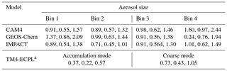
a The median correction factors for the corresponding bins 1–4 are 0.134, 0.692, 1.257 and 1.81, respectively (see text).
For TM4-ECPL, which uses modal size distributions for dust (see Table 2), we also redistributed the fine and coarse aerosols into four bins, in order to apply the same methodology. Specifically, the new aerosol modes are recalculated using the error function and based on the characteristic (radius and sigma lognormal) of each mode (see Table 2) to derive binned data for the following bin diameters: bin 1, 0–1 µm; bin 2, 1–4 µm; bin 3, 4–10 µm; and bin 4, 10–20 µm. This bias correction indicates biases mainly in the small modes, with the median correction factors for bins 1–4 being 0.134, 0.692, 1.257 and 1.81, respectively. Note also that for the ensemble model calculations of this study, the TFe and LFe depositions fluxes were calculated as the sum of Fe from the corrected mineral dust and the mean combustion aerosols.
2.3 Iron atmospheric observations
To evaluate the models' ability to reproduce the observed distributions of surface TFe and LFe aerosol concentrations over oceans, the model results were compared with available observations from Achterberg et al. (2018), Baker et al. (2006a, b, 2007, 2013), Baker and Jickells (2017), Bowie et al. (2009), Buck et al. (2006, 2010, 2013), Clifton S. Buck (personal communication, 2018), Chance et al. (2015), Gao et al. (2013), Guieu et al. (2005), Cécile Guieu (personal communication, 2018), Jickells et al. (2016), Kumar et al. (2010), Longo et al. (2016), Powell et al. (2015), Shelley et al. (2015, 2018), Sholkovitz et al. (2012), Srinivas et al. (2012), Srinivas and Sarin (2013), Wagener (2008) and Wagener et al. (2008). A total of 818 observations of TFe and 795 daily observations of LFe over the ocean performed from September 1999 to March 2015 were used for this purpose. The global distribution of the observed aerosol Fe-concentrations used for this study is presented in Fig. S3 and the respective coordinates are shown in Table S3. A bulk dust deposition flux data set compiled by Albani et al. (2014) is also used for the comparison of the Fe deposition flux after multiplying the flux by the averaged Fe content in upper crustal minerals which was 3.5 %.
TFe values were obtained from sampling aerosols in air mainly on board oceanographic cruises, and for some studies at sampling stations located on shore or on islands with no local anthropogenic influence. A variety of samplers (small or high volume) were used to collect particulate Fe, using different types of filters. TFe was either measured on whole filters or parts of filters by X-ray fluorescence or after acid digestion. LFe was obtained following several protocols, e.g., contact time, volume of media and type of media (ultra-pure water or filtered surface seawater for different pH conditions and various amounts of Fe ligands). As highlighted in Baker and Croot (2010), these diverse experimental approaches used for the determination of aerosol Fe solubility cause part of the variability observed. Although there is still no consensus regarding the experimental method to determine LFe, this data set provides valuable and robust data in all oceanic regions to be compared with model outputs. Here the results from the different protocols are all combined. Overall, the results are analyzed with regard to the role of the different model complexities, providing insight into directions for future model improvements.
3.1 Global budgets
All participating models have submitted results to enable the analysis of the TFe and LFe global budgets and atmospheric concentrations, for both dust and combustion aerosols, emissions, dry and wet deposition fluxes, atmospheric processing and atmospheric loads (see Sect. 2). Concerning the temporal resolution, daily mean spatially resolved budget terms have been submitted for IMPACT, while for GEOS-Chem, CAM4 and TM4-ECPL monthly mean fields for all budget terms are provided. However, for atmospheric concentrations all models provided daily mean fields. Concerning the aerosol size distribution (see Table 2), IMPACT and CAM4 submitted budget fields for four size bins, TM4-ECPL for two size modes and GEOS-Chem provided results as bulk aerosols. CAM4 and TM4-ECPL submitted separate fields for proton and oxalate Fe solubilization, while IMPACT and GEOS-Chem provided total fields. IMPACT and CAM4 also submitted atmospheric processing terms for dust and combustion aerosols, while TM4-ECPL only submitted terms for dust aerosols as no solubilization processes are calculated for Fe combustion aerosol in the model. GEOS-Chem does not take Fe from combustion aerosols into account.
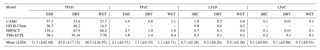
Table 4Annual budgets (Tg Fe yr−1) of total (TFe) and labile (LFe) Fe for emissions (EMI), dry deposition (DRY), wet deposition (WET) and sources (SRC; i.e., the sum of emissions and atmospheric processing) for dust (TFeD, LFeD) and combustion (TFeC, LFeC) Fe-containing aerosols as calculated by the models, as well as the models' mean (± standard deviation; SD).
3.1.1 Iron sources and deposition
The computed TFe and LFe emissions and the deposition fluxes for all models are presented in Table 4. Note, however, that for LFe (both from mineral dust and combustion sources) the total sources (the sum of primary and secondary sources) are discussed here rather than just the primary emissions. The models use significantly different assumptions to describe the total LFe source to the atmosphere and therefore primary (emissions) and secondary (atmospheric processing) sources cannot be accurately separated from rapid formation assumed in coarse-scale models. The computed annual TFe emissions and LFe sources (emissions and atmospheric processing) from (1) mineral dust and (2) combustion sources for each model are presented in Table 4, and the corresponding global emission/sources distributions are shown in Figs. S4 and S5, respectively.
Table 5Annual deposition fluxes (Tg Fe yr−1) to different ocean basins of total (TFe) and labile (LFe) Fe, as calculated by the contributing models and the derived ensemble model.
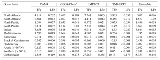
a In GEOS-Chem, only the Fe from mineral dust is considered
The importance of wet versus dry deposition as removal processes for atmospheric aerosols depends on the aerosol solubility and size distribution (and the presence/amount of precipitation). However, focusing on the deposition to oceans for this study, the apportionment of the total atmospheric deposition within different oceanic regions is presented in Table 5 (for this deposition analysis in this study we use the ocean classification as provided by HTAP phase-2: available online via the HTAP Wiki). Moreover, the combined computed annual deposition flux distributions of TFe and LFe from mineral dust and combustion sources for each model are presented in Fig. S6.
Overall, the Fe sources and deposition in the models are classified here as follows:
-
Total Fe: The modeled annual mean emission fluxes of TFe from mineral dust (TFeD) are calculated to be in the range of 38–134 Tg Fe yr−1. CAM4 and GEOS-Chem calculate similar annual TFeD emission fluxes (around 57 Tg Fe yr−1), TM4-ECPL emissions are about 40 % lower (∼38 Tg Fe yr−1) and IMPACT is about 2.4 times higher (around 134 Tg Fe yr−1). Note that IMPACT takes the largest flux among the participating models into account (Table S1), mainly due to the largest upper size. However, dust fluxes in the same size range for the different models are comparable after the bias correction based on the analysis by Kok et al. (2017) (see Sect. 2.2). TFe emissions from combustion sources (TFeC) range between 1.8 and 2.7 Tg Fe yr−1, with CAM4 and TM4-ECPL calculating annual mean fluxes of around 1.8 Tg Fe yr−1 globally, and IMPACT having a 35 % higher estimate. On a global scale, dry deposition is the most important removal mechanism, across all models for the TFeD; IMPACT has the highest dry deposition flux of all models (∼68 Tg Fe yr−1), followed by GEOS-Chem (∼40 Tg Fe yr−1), CAM4 (∼33 Tg Fe yr−1) and TM4-ECPL (∼30 Tg Fe yr−1). Submicron aerosols are mostly removed by wet removal, while for supermicron aerosols the gravitational settling is important (e.g., Seinfeld and Pandis, 2006). Consequently, the wet removal of TFeD across almost all models (except for IMPACT) is smaller than dry deposition flux – mainly due to the high contribution of coarse aerosol sedimentation to the dry removal processes (Table 4). The simulated wet deposition flux of TFeD ranges over about 1 order of magnitude (from about 8 to 66 Tg Fe yr−1); IMPACT calculates the highest TFeD wet deposition flux of all models of about 66 Tg Fe yr−1 (∼49 % of total removal), followed by CAM4 (24 Tg Fe yr−1; 42 %), GEOS-Chem (16 Tg Fe yr−1; ∼29 %) and TM4-ECPL (roughly 8 Tg Fe yr−1; ∼20 %). In contrast to TFeD, due to the similar assumptions of the size distribution and scavenging efficiency in the models, the wet deposition is the larger removal pathway for TFe from combustion processes (TFeC), (except for in TM4-ECPL, probably due to the different solubility factors in primary emissions and the different atmospheric processing parameterizations), and is responsible for about 60 % of the overall total TFeC removal across models which amounts to about 1 Tg Fe yr−1.
-
Labile Fe: The global annual mean LFe sources from mineral dust (LFeD) range between 0.3 and 1.0 Tg Fe yr−1. IMPACT and GEOS-Chem calculate similar LFeD sources, close to 0.7–0.8 Tg Fe yr−1, whereas CAM4 calculates the highest annual source and TM4-ECPL the lowest. However, these differences are mainly attributed to the secondary processes leading to LFeD production rather than the primary emissions. For example, despite the large difference between IMPACT and TM4-ECPL regarding TFeD sources, the models consider similar LFeD emissions amounts ranging between 0.12 and 0.13 Tg Fe yr−1. In contrast, the secondary LFeD produced due to atmospheric processing is calculated to vary by a factor of 3–4 between 0.57 Tg Fe yr−1 (IMPACT) and 0.17 Tg Fe yr−1 (TM4-ECPL), respectively. CAM4 takes LFeD emissions of around 0.18 Tg Fe yr−1 into account and displays the highest annual LFeD atmospheric processing (0.8 Tg Fe yr−1), whilst GEOS-Chem presents values of about 0.25 and 0.54 Tg Fe yr−1 for LFeD emissions and atmospheric processing, respectively. The LFe source from combustion aerosols (LFeC), with a range of about 0.1–0.2 Tg Fe yr−1, shows smaller differences than that of mineral dust (0.3–1.0 Tg Fe yr−1). Although the differences are not large, they clearly depict the different assumptions followed by these two models: IMPACT does not account for primary LFe sources from combustion (expect those from oil ship combustion of about 0.009 Tg Fe yr−1), meaning that almost all of the LFeC sources over land are attributed to secondary production via atmospheric processing (0.091 Tg Fe yr−1). In contrast, TM4-ECPL does not take atmospheric processing of Fe from combustion sources into account, and attributes all the LFeC sources to direct emissions (∼0.2 Tg Fe yr−1). Finally, the CAM4 model, which includes both direct emissions and atmospheric processing of LFeC, calculates a total source of about 0.13 Tg Fe yr−1, corresponding to roughly 0.075 and 0.053 Tg Fe yr−1, for primary LFeC emissions and atmospheric processing, respectively.

Figure 1Seasonal LFe sources (positive bars) and oceanic deposition fluxes (negative bars/pale colors) in Tg Fe season−1 for December, January and February (DJF); March, April and May (MAM); June, July and August (JJA); and September, October and November (SON), as calculated by each model (CAM4, magenta; GEOS-Chem, red; IMPACT, green; and TM4-ECPL, blue), as well as, the ensemble model (yellow). The hatched areas correspond to the combustion aerosols and the error bars correspond to the standard deviation of the respective season.
3.1.2 Iron seasonal variability
Figure 1 presents the global LFe sources (positive) and oceanic deposition fluxes (negative) for all participating models and their ensemble mean (see Sect. 3.2), for the four seasons, i.e., December, January and February (DJF); March, April and May (MAM); June, July and August (JJA); and September, October and November (SON). LFe sources are mainly driven by mineral dust aerosols, although a significant fraction (6 % – 62 %) is due to LFe combustion aerosols, especially over the high-latitudes of the Northern Hemisphere (Ito et al., 2018b). For LFe sources, despite the different assumptions applied in the models (i.e., atmospheric processing and direct LFe emissions), maximum sources are calculated for MAM and JJA due to intense dust emissions and biomass burning, respectively. The models with the highest LFe sources, also exhibit the highest deposition fluxes to the ocean. However, significant differences in the magnitude of the deposition fluxes are calculated between models (Fig. 1). A seasonal maximum in the deposition fluxes is calculated by CAM4 and GEOS-Chem during MAM, attributed to Saharan mineral dust aerosols, while IMPACT and TM4-ECPL present a seasonal maximum during JJA.
Figure S7 (Supplement) further presents the zonal mean seasonal variability of the LFe global sources and oceanic deposition fluxes. Most of LFe emissions are calculated to occur over the midlatitudes of the Northern Hemisphere (NH) for all seasons, with a maximum during MAM and JJA and minima during SON. In DJF, and to a lesser extent in JJA, two zonal maxima are shown near the Equator and around 30∘ N. However, the equatorial maximum in DJF is shifted to the Northern Hemisphere in JJA following the intertropical convergence zone (ITCZ) migration and the subsequent geographic change in the location of biomass burning emissions. Again, all models appear to have similar LFe seasonality, with the highest LFe oceanic deposition fluxes across all models calculated by CAM4 (Table 5).
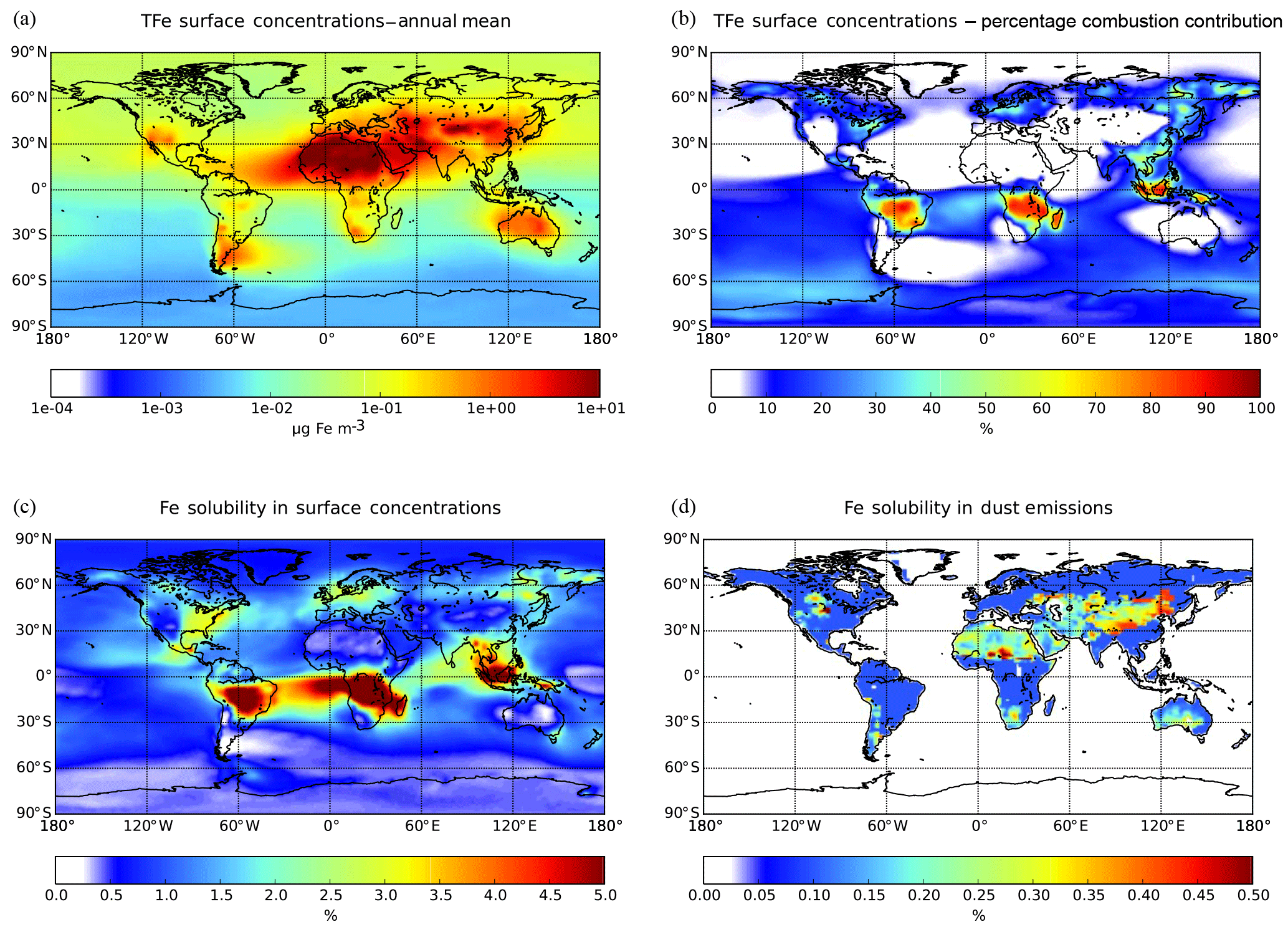
Figure 2Ensemble model results for annual mean (a) surface TFe concentration (µg m−3), (b) the percentage contribution of Fe-containing combustion aerosols, (c) the Fe solubility (%) in surface TFe concentration and (d) the initial solubility (%) in Fe-containing dust emissions.
3.2 Ensemble model calculations
3.2.1 Iron surface concentrations
The annual mean surface TFe aerosol concentrations for the ensemble model exceed 100 µg Fe m−3 over the major dust source regions such as the Sahara Desert, where mineral dust particles dominate the atmospheric Fe burden (Fig. 2a). Relatively high TFe concentrations (e.g., up to 10 µg Fe m−3 over the tropical Atlantic Ocean) are calculated for ocean regions at the outflow from these source regions. High TFe concentrations of around 6 µg Fe m−3 are also calculated over heavily polluted areas like China, while secondary maxima up to 2–5 µg Fe m−3 are calculated over central Africa, Asia and Indonesia, where Fe-containing aerosols are associated with biomass burning emissions (Fig. 2b).
Model Fe solubility calculations (Fig. 2c) clearly suggest the impact of atmospheric processing on the derived LFe ensemble surface concentrations, with high Fe solubilities calculated far from source regions over the remote tropical oceans, corresponding to low TFe concentrations. Ensemble annual mean LFe concentrations of around 0.5 µg Fe m−3 occur downwind of the Sahara and of around 0.1 µg Fe m−3 downwind of the Arabian and Gobi deserts. At the outflow of these regions, the Fe solubility over the global ocean is calculated to be about 1 %–1.5 %, with the highest Fe solubilities (4 %–5 %) over the tropical Atlantic Ocean (Fig. 2c). Additionally, LFe concentrations over polluted regions may range up to 0.05 µg Fe m−3, indicating a significant anthropogenic contribution via direct combustion emissions and atmospheric processing (Fig. 2b). Over central South America, Asia and Indonesia, LFe concentrations of about 0.03–0.05 µg Fe m−3 (corresponding to high Fe solubilities up to 5 %) are found due to both direct biomass-burning emissions and due to ligand-promoted dissolution. The latter process is enhanced in these areas by the respective enhanced oxalate production upon the oxidation of emitted biogenic VOCs precursors, such as isoprene, under cloudy conditions (Lin et al., 2014; Myriokefalitakis et al., 2011).
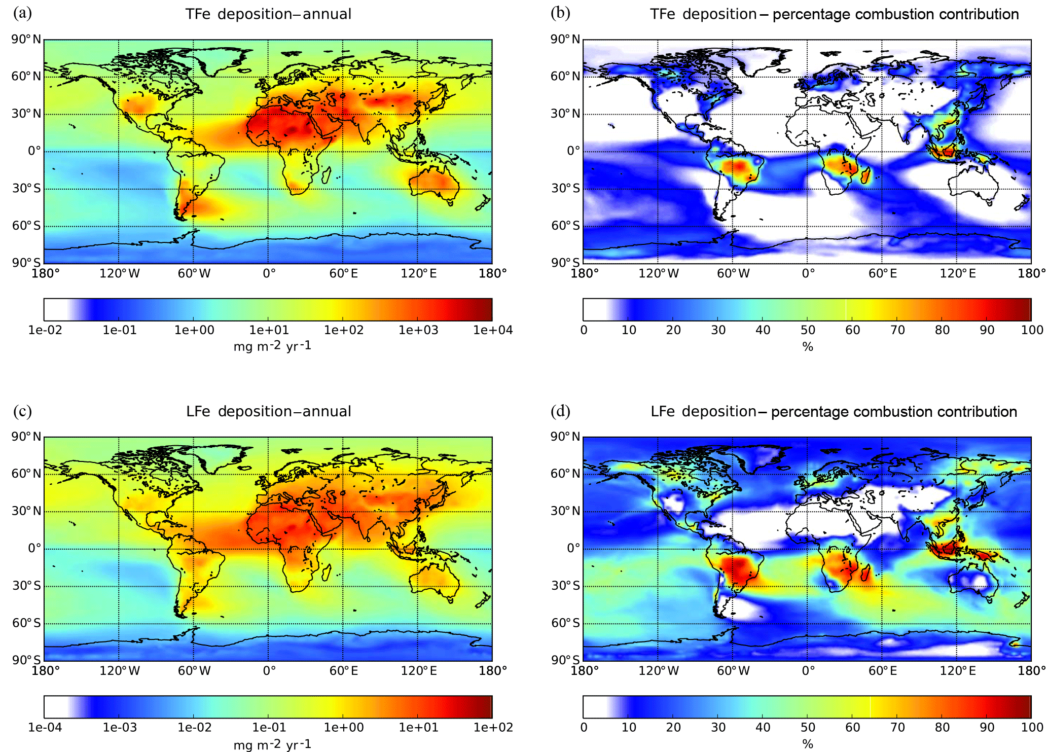
Figure 3Ensemble model results for annual deposition fluxes () for (a) TFe and for (c) LFe and their respective percentage contribution of combustion aerosols (b, d).
3.2.2 Iron deposition fluxes
Model calculations indicate that about 71.5 (±43) Tg Fe yr−1 of TFe from mineral dust are deposited to the Earth's surface (Table 4), with ensemble deposition fluxes of around 5000–8000 calculated downwind of the main desert source regions (Fig. 3a). However, within the northern Atlantic Ocean in the outflow of the Sahara, the model mean indicates deposition fluxes up to 2400 , while within the northern Pacific Ocean in the outflow of Gobi Desert and within the Southern Ocean downwind of the Patagonia Desert the ensemble model shows annual mean fluxes of ∼34 and ∼10 , respectively (Fig. 3a). The TFe annual mean global deposition flux from combustion sources (Table 4) is calculated to be about 2.2 (±0.5) Tg Fe yr−1, with two main regions where TFe concentrations exceed 2500 , one near biomass burning regions (e.g., southern Africa, South America and Southeast Asia) with up to ∼3000 , and a second near highly populated regions with Fe released from coal and oil combustion processes (India and China) with up to ∼3500 (Fig. 3b).
A global mean LFe deposition flux of 0.7 (±0.2) Tg Fe yr−1 is derived from all models (Table 4), with about one-third (∼0.24 Tg Fe yr−1) calculated to be deposited to the global ocean for the ensemble model (Table 5). The highest annual mean LFe deposition fluxes (up to 36 ) are simulated within dust source regions (Fig. 3c), mainly owing to the LFe content of the emissions (e.g., see Fig. 2d). The global model-mean LFe deposition fluxes from combustion sources are calculated at about 0.2 (±0.04) Tg Fe yr−1 (Table 4), with maximum global deposition rates of 4–5 (Fig. 3c) simulated in the outflow of tropical biomass burning regions (i.e., South America, Africa and Indonesia), clearly reflecting the contribution of combustion processes. Focusing on the marine environment, annual mean LFe deposition rates of 15 are calculated for the tropical Atlantic Ocean and for the Indian Ocean (up to 16 ) under the influence of the Arabian and Indian peninsulas, but up to ∼29 for the Mediterranean Sea downwind of the Sahara Desert. Deposition rates around 1 are calculated to occur within the northern Pacific in the outflow from the Gobi Desert as well as within the Southern Hemisphere downwind of Patagonia to the Southern Ocean (up to 0.1 ) and downwind of the dust source regions of Australia and South America (up to ∼4 ). The LFe deposition rates to the Southern Ocean are mainly associated with the Patagonian, southern African and Australian deserts, with a smaller contribution in the subtropical ocean from biomass burning sources (Fig. 3d). Note, that the largest fluxes of LFe deposited to the HNLC region of the Southern Ocean (e.g., south of the Antarctic Circumpolar Current) are simulated to be originating from a Patagonian mineral dust source, with rates reaching 0.1 . The ensemble annual mean deposition fluxes to various oceanic regions are further presented in Table 5.

Figure 4Comparison of simulated and observed TFe concentrations (ng m−3), Fe solubility (%) and LFe concentrations (ng m−3) in the Northern Hemisphere (blue circles) and Southern Hemisphere (red squares) for (a, b, c) CAM4, (d, e, f) GEOS-Chem, (g, h, i) IMPACT, (j, k, l) TM4-ECPL, and (m, n, o) the ensemble model. The mean normalized biases (MNB) between the models and observations are presented in parentheses. The solid line represents a 1:1 correspondence and the dashed lines show the 10:1 and 1:10 relationships, respectively. The bias correction in the mineral dust size distribution is applied for the comparison with field data (Kok et al., 2017).
4.1 Comparison with measurements
The TFe concentrations, Fe solubility and LFe concentrations from the models are compared with the measurements and presented in Fig. 4. We use the monthly mean of the model output to compare with the measurements. The normalized bias (NB) at a given grid box is calculated as follows:
where Cmodel,i is the modeled aerosol concentration in grid box i and Cobs,i is the measured aerosol concentration in the same grid box. When discussing the multi-model results we use the mean of all models, while we also analyze the mean normalized bias (MNB) of the models against measurements (a perfect comparison would have an MNB of 0 and correlation, R, of 1). A model's MNB is derived as the arithmetic mean of all NBi values; thus, overestimates are weighted more than equivalent underestimates.

Figure 5Fe solubility versus atmospheric concentrations of aerosol Fe (ng m−3) in the Northern Hemisphere (blue circles) and Southern Hemisphere (red squares) for (a) the measurements, (b) CAM4, (c) GEOS-Chem, (d) IMPACT, (e) TM4-ECPL and (f) the ensemble model. The bias correction in the mineral dust size distribution is applied for the comparison with field data (Kok et al., 2017).
All models captured a tendency for higher Fe concentrations near and downwind of the major dust source regions. The MNB for the Northern Hemisphere (14 for ensemble model) is larger than that for the Southern Hemisphere (2.4 for ensemble model). This reflects that the models generally overestimate TFe surface mass concentrations. However, from Fig. 4 we can see that this overestimate is higher for the highest TFe concentrations near the dust source regions and tends to become an underestimate for the lowest concentrations observed over remote oceans. Overall, bias correction for the ensemble model improves the agreement of the ensemble model against measurements (Fig. S8). However, we note that matching the atmospheric concentrations may cause a high bias in the simulated Fe depositions at low values in the Southern Hemisphere (Albani et al., 2014; Huneeus et al., 2011) (Fig. S9). The computed correlation coefficients of the ensemble model against measurements at the surface are 0.13 for TFe, 0.05 for Fe solubility and 0.25 for LFe, respectively, which are much smaller than those between the participating models: 0.57–0.90 for TFe (GEOS-Chem vs. IMPACT)–(CAM4 vs. TM4-ECPL), 0.05–0.56 for Fe solubility (CAM4 vs. TM4-ECPL)–(CAM4 vs. IMPACT), and 0.40–0.75 for LFe (GEOS-Chem vs. IMPACT)–(CAM4 vs. GEOS-Chem). This indicates a linear dependence of the model results and that the models have similar behavior accounting for the same key processes that affect Fe deposition. The small positive correlation between models and observations indicates that the models miss – or do not accurately represent – important processes that drive the variability in the observations. Indeed, when comparing the computed and observed solubilities of Fe, all models overestimate the lowest solubilities (<0.1 %) observed close to the source regions (14 samples in the Arabian Sea and 2 samples in the tropical Atlantic). This is primarily due to the assumed solubility of the dust aerosols at emissions, and the subsequent enhancement of Fe solubility estimated from the simulated amount of atmospheric processing during transport in the models. However, it is noted that the lowest solubilities in the measurements are outliers in the negative slope of Fe concentrations versus Fe solubility in the Northern Hemisphere (Fig. 5). Our calculations show that the models have difficulties simulating the 4 orders of magnitude variability from 0.02 % to 98 % in the Fe solubility observed in the atmosphere (Fig. 5a). IMPACT simulates almost 3 orders of magnitude variability in Fe solubility. In the other models, including the ensemble model, Fe solubility is less variable (only 1–2 orders of magnitude). In particular, low solubilities (high concentrations near sources) are overestimated and high solubilities (low concentrations at remote locations) are underestimated. This may indicate that the primary LFe in the models is overestimated and that models are missing solubilization processes during transport or that those considered in the models are not sufficiently effective.
All models underestimate the high end of the observed values (>10 %) in the Southern Ocean, which are mainly associated with transported and aged aerosols; this may be a significant shortcoming because the Southern Ocean is an oceanic HNLC region where the atmospheric Fe supply has a potentially important impact on ocean productivity in past and future climate. In GEOS-Chem, IMPACT and TM4-ECPL, Fe dissolution over the Southern Ocean is mainly suppressed due to the lack of anthropogenic emissions and the subsequent acidification of the aerosols. CAM4 is relatively insensitive to the acidity, as most labile Fe is formed via in-cloud processes. Thus, the model results from CAM4 can in part test whether in-cloud processing can realistically describe the observed pattern of solubility over the Southern Ocean. CAM4 shows higher Fe solubility than field data for most samples in the Southern Ocean (69 % in CAM4, 7 % in GEOS-Chem, 55 % in IMPACT and 5 % in TM4 TM4-ECPL; Figs. 4 and 5). Thus, the wide range of observed Fe solubility cannot be explained by excluding the effect of modeled aerosol acidity over the Southern Ocean. It is worth mentioning that IMPACT, which has the highest complexity in simulating labile Fe, reproduces the widest range of observed Fe solubility. However, it should be noted that the comparison of monthly mean model results with the shorter-term (e.g., daily) observations during different sampling periods introduces inaccuracies due to the episodic nature of high Fe solubility. A more detailed comparison of Fe solubility between models and observations is presented in a separate companion paper to this work (Ito et al., 2018b).
4.2 Model-to-model comparison
Model budget analysis and model evaluation indicate that even though the models are able to reproduce surface Fe measurements to some extent, large differences exist among modes in processes such as emissions, transport and deposition. A large diversity is documented here between models in terms of LFe primary sources (i.e., emissions) and secondary processes (i.e., atmospheric processing) which introduce uncertainties in the estimated oceanic deposition. However, there are many intrinsic reasons for this diversity in the Fe simulations among models: besides the emitted Fe mass in the atmosphere (especially from dust aerosols), the aerosol size distribution, the soil mineralogy, the strength of combustion aerosol sources, as well as the parameterizations used to calculate the pH of the aerosol water and the oxalate production are large sources of uncertainty in model simulations.
The aerosol size and solubility are important factors driving the atmospheric cycle of Fe, as they both control the removal processes from the atmosphere via the dry deposition (including gravitational settling) and the wet scavenging (e.g., Albani et al., 2014). It is well documented that the lifetime of Fe-containing aerosols ranges between less than 1 day for the coarse mode (with diameters larger than 1 µm) particles to weeks for the fine mode (with diameters less than 1 µm) (e.g., Ginoux et al., 2012; Luo et al., 2008; Mahowald et al., 2009; Tegen and Fung, 1994), with the overall lifetime of dust aerosols usually ranging between 1.6 and 7.1 days in the models (Huneeus et al., 2011). Fine particles have longer lifetimes and thus experience more atmospheric processing. The conversion of insoluble mineral content to soluble forms as the result of aging during atmospheric transport increases aerosols' solubility. Lifetime calculations can thus provide a valuable tool to determine the Fe persistence in the atmosphere, overall integrating sources, transport and deposition differences among models, especially over remote areas such as the open ocean.
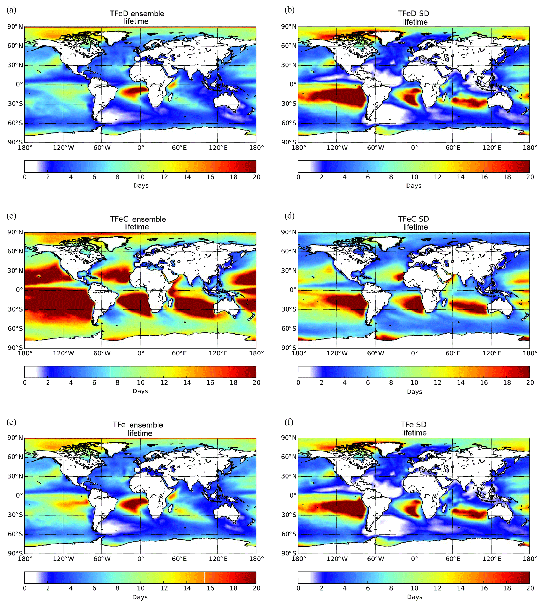
Figure 6Ensemble model results for TFe lifetime (days) over the ocean having originated from (a) mineral dust sources, (c) combustion source, and (e) total (mineral dust + combustion) and the respective standard deviation (b, d, f). Lifetimes are atmospheric concentrations divided by total sinks.
Figure 6 presents the spatial distribution of the TFe lifetime over the ocean (i.e., atmospheric concentrations divided by total sinks), as calculated for the ensemble model. For TFe originating from dust sources, the calculated global mean lifetime over the oceans is ∼6 (±4) days (Fig. 6a). The lifetime of combustion TFe over oceans is longer, at around 14 (±9) days (Fig. 6c), due to the generally smaller size of the combustion Fe aerosols compared to that of mineral dust (affecting their sedimentation processes and their horizontal and vertical transport in the atmosphere), but also because of the low precipitation over part of the regions in which mineral dust and combustion aerosols are transported. The ensemble model indicates long TFe lifetimes over remote oceanic regions, such as in the outflow of South America, in the outflow of South Africa and the outflow of Australia (Fig. 6c). Over these so-called “ocean deserts”, where precipitation is low and thus the wet deposition rates are low, the ensemble model generally results in longer lifetimes for Fe-containing aerosols, although the LFe atmospheric concentrations can be extremely low.
To further analyze the differences among the models, the standard deviation (SD) of the TFe lifetime is calculated for each grid for dust aerosols (Fig. 6b), combustion aerosols (Fig. 6d) and the combined TFe lifetime (Fig. 6f). Over remote oceanic regions, the high SD can be related to the different assumptions used by the models to parameterize (1) the long-range transport of Fe-containing aerosols of different parameterizations of the sizes, (2) the wet and dry deposition parameterizations and (3) the soluble fraction of Fe-containing combustion aerosols (e.g., the differences in ship oil combustion and biomass burning emissions). From the models that include Fe from combustion processes, IMPACT assumes that only ship oil combustion emissions have an initial fraction of soluble Fe; thus, all the LFe from continental sources is produced due to atmospheric processing. CAM4 does not take ship emissions into account but includes both primary and secondary sources for LFe from other combustion sources. TM4-ECPL, in comparison, includes continental and ship oil combustion emissions for both TFe and LFe, but it does not take any dissolution processes for combustion aerosols into account, although continental and ship oil combustion emissions both for TFe and LFe are considered. Differences in the precipitation patterns or parameterization for wet or dry deposition in the models can also partially explain the models' diversity. In addition, less constrained parameters like dissolution, long-range transport and Fe removal (which affect Fe solubility) can further increase the model diversity, and in turn the SD, over these remote areas.
Here we present the first model intercomparison study of the atmospheric Fe-cycle by assessing aerosol simulations of total and labile Fe using four state-of-the-art global aerosol models (CAM4, IMPACT, GEOS-Chem and TM4-ECPL). The TFe emissions from dust sources in the models range from ∼38 to ∼134 Tg Fe yr−1, with a mean value of 71.5 (±43) Tg Fe yr−1. The models simulate the secondary formation of soluble Fe in the atmosphere, as a result of mineral Fe atmospheric processing by acids, organic ligands and photochemistry, but the absolute amount of the simulated LFe remains highly uncertain. The simulated LFe deposition fluxes from mineral dust span from 0.3 to 1.0 Tg Fe yr−1, with a mean value of around 0.7 (±0.3) Tg Fe yr−1. All models capture the main features of the distribution of TFe and LFe, i.e., the large deposition rates to the Sahara and Gobi deserts and regions downwind of strong dust sources. Models also show significant LFe deposition to the oceans downwind from the Middle East and the continents of South America, Africa and Australia in the Southern Hemisphere; the Middle East has large dust sources, while South America, Africa and Australia experience strong biomass burning emissions.
The models are able to simulate the main features of TFe and LFe atmospheric concentrations and deposition fluxes. On average, the ensemble model computes a roughly 50 % higher lifetime with respect to the deposition flux for combustion aerosol (∼14 days) than for dust aerosol, reflecting differences in the size distribution and the location of the emitted aerosols. Ensemble model calculations present an overestimate of the observed TFe surface mass concentrations near the dust source regions and underestimate the Fe concentrations over the Southern Ocean compared with cruise measurements; similar to what was pointed out in Albani et al. (2014) and seen in the dust model intercomparison study of Huneeus et al. (2011). Note that the latter is important because of the key role of Fe in the biogeochemistry of these ocean waters. For the ensemble model mean, the MNB for the Northern Hemisphere (about 14) is larger than for the Southern Hemisphere (about 2.4). Note, however, that the evaluation of monthly mean model results by comparison with the shorter-term (e.g., daily) observations during different sampling periods introduces uncertainties, due to the short sampling frequencies; a comparison of long-term measurements with a multi-year modeling would allow for the assessment of the model performance regarding the capture of labile Fe concentrations under specific events.
The model intercomparison and model–observation comparison revealed the Fe size distribution and the relative contribution of the dust and combustion sources to be two critical issues for LFe simulations that now require further study. Thus, the diversity of how the models represent Fe emissions as well as of deposition fluxes among the models can be large, especially over source regions. The model diversity over remote oceans reflects uncertainty in the Fe content parameterizations of dust emissions (e.g., soil mineralogy and the initial Fe soluble content in primary sources) and combustion aerosols, and/or in the parameterizations of the size distribution of the transported aerosol Fe, and in turn the representation of deposition fluxes – which generally control the atmospheric lifetime of Fe. Conversely, there are many other intrinsic reasons for this diversity, especially for the LFe aerosol fraction, as it involves complex atmospheric chemical processes driven by atmospheric acidity. For example, detailed chemical mechanisms need to be invoked to simulate a multi-phase, multi-component solution system, since such a system may not be accurately solved using a thermodynamic equilibrium approach for the entire grid box due to sub-grid processes, e.g., when the dust plume is not well mixed with surrounding pollutants. Consequently, a reasonable aerosol pH simulation further depends on the representation of soluble acidic and basic compounds, as well as the water content of hygroscopic particles.
In this respect, new field observations are needed to improve the understanding of the Fe solubilization process, and how this process alters in the presence of anthropogenic pollution. Modeling studies and their evaluation based on a greater number of atmospheric observations, especially over the remote ocean regions, are deemed necessary in order to reduce the uncertainty associated with the model performance in simulating the atmospheric Fe deposition. For example, the participating models in this study predict that wet deposition processes are important for the LFe atmospheric cycle; however, this is rather hard to test well, due to the lack of respective field data. Moreover, although the models do well in higher dust and pollution regions, from an oceanographer's perspective, the regions with the lowest Fe supply are of greatest interest, due to the creation of HNLC situations in the water column. However, model evaluation can also be difficult due to the lack of standardization in the protocols used to determine the soluble Fe fraction in marine aerosol samples (e.g., Baker and Croot, 2010). Protocols that involve different solutes, aerosol–solution contact times and filter pore sizes, among other differences, are used by different investigators and these presumably introduce some, as yet unquantified, uncertainties into the available databases of aerosol soluble Fe concentrations and Fe solubility. Model developments related to the atmospheric Fe cycle must be performed in parallel with an extensive model evaluation in order to better understand the underlying mechanisms and to provide, overall, realistic labile Fe deposition fluxes for the next generation of ocean biogeochemistry modeling studies. Although the calculation of the Fe concentrations in the ocean is outside the scope of this paper, we expect that the Fe deposition fluxes here provided will be used in oceanic models.
Global 1.0×1.0 fields for TFe and LFe deposition fluxes (i.e., from combustion and dust origin and their sum) as well as the Fe solubility (SFe) derived from the ensemble model calculations are available online at https://ecpl.chemistry.uoc.gr/GESAMP/, last access: 5 November 2018 (contact: Stelios Myriokefalitakis, steliosm@noa.gr; Maria Kanakidou, mariak@uoc.gr).
The supplement related to this article is available online at: https://doi.org/10.5194/bg-15-6659-2018-supplement.
This paper resulted from the deliberations of United Nations GESAMP Working Group 38, “The Atmospheric Input of Chemicals to the Ocean” (SM, AI, MK, AN, NMM, ARB, TDJ, MMS, RS, MMGP, CG, RAD), February 2017, University of East Anglia, Norwich, UK. SM manipulated all model fields, analyzed the data and prepared the respective figures and fields of this work. AI performed the model evaluation and the respective statistical analysis. JFK provided the analysis for dust correction factors for model data. SM, AI, MK, MCK, AN, NMM, RAS, DSH, NM and MSJ, provided the model products. ARB, TDJ, MMS, SB, RS, and CG contributed to the measured data. All authors contributed to the preparation of the paper.
The authors declare that they have no conflict of interest.
Stelios Myriokefalitakis acknowledges financial support for this research from the
European Union's Horizon 2020 research and innovation programme under the
Marie Skłodowska-Curie grant agreement no. 705652 – ODEON. Support for this
research was provided to Akinori Ito by JSPS KAKENHI grant no. JP16K00530 and
the Integrated Research Program for Advancing Climate Models (MEXT). Natalie M. Mahowald, Rachel A. Scanza and
Douglas S. Hamilton acknowledge support from a Department of Energy grant (DE-SC0006791CE14).
Andrew Bowie and Morgane M. G. Perron were
funded by an Australian Research Council Future Fellowship (FT130100037). We
are grateful to Thibaut Wagener for kindly providing the field data set. This work is
prepared in the framework of the Joint Group of Experts on the Scientific
Aspects of Marine Environmental Protection (GESAMP; http://www.gesamp.org/, last access: 5 November 2018),
Working Group 38, the Atmospheric Input of
Chemicals to the Ocean. We thank the Global Atmosphere Watch and the World
Weather Research Programme of the World Meteorological Organization, the
International Maritime Organization, the U.S. National Science Foundation,
the ICSU Scientific Committee on Oceanic Research (SCOR) and the University
of East Anglia for their financial support. We also thank SOLAS for their sponsorship.
Data post-processing was carried out on the Dutch national e-infrastructure
with the support of the SURF Cooperative. The publication of this work was
financed by Utrecht University and by the European Union's Horizon 2020
research and innovation programme under the Marie Skłodowska-Curie grant
agreement no. 705652 – ODEON.
Edited by: Maria Tzortziou
Reviewed by: two anonymous referees
Achterberg, E. P., Steigenberger, S., Marsay, C. M., Lemoigne, F. A. C., Painter, S. C., Baker, A. R., Connelly, D. P., Moore, C. M., Tagliabue, A., and Tanhua, T.: Iron Biogeochemistry in the High Latitude North Atlantic Ocean, Sci. Rep.-UK, 8, 1283, https://doi.org/10.1038/s41598-018-19472-1, 2018.
Albani, S., Mahowald, N. M., Perry, A. T., Scanza, R. A., Zender, C. S., Heavens, N. G., Maggi, V., Kok, J. F., and Otto-Bliesner, B. L.: Improved dust representation in the Community Atmosphere Model, J. Adv. Model. Earth Syst., 6, 541–570, https://doi.org/10.1002/2013MS000279, 2014.
Baker, A. R. and Croot, P. L.: Atmospheric and marine controls on aerosol iron solubility in seawater, Mar. Chem., 120, 4–13, https://doi.org/10.1016/j.marchem.2008.09.003, 2010.
Baker, A. R. and Jickells, T. D.: Mineral particle size as a control on aerosol iron solubility, Geophys. Res. Lett., 33, L17608, https://doi.org/10.1029/2006GL026557, 2006.
Baker, A. R. and Jickells, T. D.: Atmospheric deposition of soluble trace elements along the Atlantic Meridional Transect (AMT), Prog. Oceanogr., 158, 41–51, https://doi.org/10.1016/j.pocean.2016.10.002, 2017.
Baker, A. R., French, M., and Linge, K. L.: Trends in aerosol nutrient solubility along a west–east transect of the Saharan dust plume, Geophys. Res. Lett., 33, L07805, https://doi.org/10.1029/2005GL024764, 2006a.
Baker, A. R., Jickells, T. D., Witt, M., and Linge, K. L.: Trends in the solubility of iron, aluminium, manganese and phosphorus in aerosol collected over the Atlantic Ocean, Mar. Chem., 98, 43–58, https://doi.org/10.1016/j.marchem.2005.06.004, 2006b.
Baker, A. R., Weston, K., Kelly, S. D., Voss, M., Streu, P., and Cape, J. N.: Dry and wet deposition of nutrients from the tropical Atlantic atmosphere: Links to primary productivity and nitrogen fixation, Deep Sea Res.-Pt. I, 54, 1704–1720, https://doi.org/10.1016/j.dsr.2007.07.001, 2007.
Baker, A. R., Adams, C., Bell, T. G., Jickells, T. D., and Ganzeveld, L.: Estimation of atmospheric nutrient inputs to the Atlantic Ocean from 50∘ N to 50∘ S based on large-scale field sampling: Iron and other dust-associated elements, Global Biogeochem. Cy., 27, 755–767, https://doi.org/10.1002/gbc.20062, 2013.
Benitez-Nelson, C. R., Vink, S. M., Carrillo, J. H., and Huebert, B. J.: Volcanically influenced Fe and Al cloud water deposition to Hawaii, Atmos. Environ., 37, 535–544, https://doi.org/10.1016/S1352-2310(02)00892-0, 2003.
Bonnet, S.: Dissolution of atmospheric iron in seawater, Geophys. Res. Lett., 31, L03303, https://doi.org/10.1029/2003GL018423, 2004.
Bowie, A. R., Lannuzel, D., Remenyi, T. A., Wagener, T., Lam, P. J., Boyd, P. W., Guieu, C., Townsend, A. T., and Trull, T. W.: Biogeochemical iron budgets of the Southern Ocean south of Australia: Decoupling of iron and nutrient cycles in the subantarctic zone by the summertime supply, Global Biogeochem. Cy., 23, GB4034, https://doi.org/10.1029/2009GB003500, 2009.
Boyd, P. W. and Ellwood, M. J.: The biogeochemical cycle of iron in the ocean, Nat. Geosci., 3, 675–682, https://doi.org/10.1038/ngeo964, 2010.
Boyd, P. W., Strzepek, R., Takeda, S., Jackson, G., Wong, C. S., McKay, R. M., Law, C., Kiyosawa, H., Saito, H., and Sherry, N.: The evolution and termination of an iron-induced mesoscale bloom in the northeast subarctic Pacific, Limnol. Oceanogr., 50, 1872–1886, https://doi.org/10.4319/lo.2005.50.6.1872, 2005.
Brandt, F., Bosbach, D., Krawczyk-Barsch, E., Arnold, T., and Bernhard, G.: Chlorite dissolution in the acid ph-range: a combined microscopic and macroscopic approach, Geochim. Cosmochim. Ac., 67, 1451–1461, https://doi.org/10.1016/S0016-7037(02)01293-0, 2003.
Buck, C. S., Landing, W. M., Resing, J. A., and Lebon, G. T.: Aerosol iron and aluminum solubility in the northwest Pacific Ocean: Results from the 2002 IOC cruise, Geochem. Geophys. Geosyst., 7, 1–21, https://doi.org/10.1029/2005GC000977, 2006.
Buck, C. S., Landing, W. M., Resing, J. A., and Measures, C. I.: The solubility and deposition of aerosol Fe and other trace elements in the North Atlantic Ocean: Observations from the A16N CLIVAR/CO2 repeat hydrography section, Mar. Chem., 120, 57–70, https://doi.org/10.1016/j.marchem.2008.08.003, 2010.
Buck, C. S., Landing, W. M., and Resing, J.: Pacific Ocean aerosols: Deposition and solubility of iron, aluminum, and other trace elements, Mar. Chem., 157, 117–130, https://doi.org/10.1016/j.marchem.2013.09.005, 2013.
Chance, R., Jickells, T. D., and Baker, A. R.: Atmospheric trace metal concentrations, solubility and deposition fluxes in remote marine air over the south-east Atlantic, Mar. Chem., 177, 1–12, https://doi.org/10.1016/j.marchem.2015.06.028, 2015.
Cheize, M., Sarthou, G., Croot, P. L., Bucciarelli, E., Baudoux, A.-C., and Baker, A. R.: Iron organic speciation determination in rainwater using cathodic stripping voltammetry, Anal. Chim. Acta, 736, 45–54, https://doi.org/10.1016/j.aca.2012.05.011, 2012.
Chen, H. and Grassian, V. H.: Iron Dissolution of Dust Source Materials during Simulated Acidic Processing: The Effect of Sulfuric, Acetic, and Oxalic Acids, Environ. Sci. Technol., 47, 10312–10321, https://doi.org/10.1021/es401285s, 2013.
Chen, H., Laskin, A., Baltrusaitis, J., Gorski, C. A., Scherer, M. M., and Grassian, V. H.: Coal Fly Ash as a Source of Iron in Atmospheric Dust, Environ. Sci. Technol., 46, 2112–2120, https://doi.org/10.1021/es204102f, 2012.
Chen, Y. and Siefert, R. L.: Seasonal and spatial distributions and dry deposition fluxes of atmospheric total and labile iron over the tropical and subtropical North Atlantic Ocean, J. Geophys. Res., 109, D09305, https://doi.org/10.1029/2003JD003958, 2004.
Chuang, P. Y., Duvall, R. M., Shafer, M. M., and Schauer, J. J.: The origin of water soluble particulate iron in the Asian atmospheric outflow, Geophys. Res. Lett., 32, L07813, https://doi.org/10.1029/2004GL021946, 2005.
Claquin, T., Schulz, M., and Balkanski, Y. J.: Modeling the mineralogy of atmospheric dust sources, J. Geophys. Res.-Atmos., 104, 22243–22256, https://doi.org/10.1029/1999JD900416, 1999.
de Baar, H. J. W. and de Jong, J. T. M.: Distributions, sources and sinks of iron in seawater, in The Biogeochemistry of Iron in Seawater, IUPAC Series on Analytical and Physical Chemistry of Environmental Systems, Wiley, New York, 123–253, 2001.
Dentener, F., Kinne, S., Bond, T., Boucher, O., Cofala, J., Generoso, S., Ginoux, P., Gong, S., Hoelzemann, J. J., Ito, A., Marelli, L., Penner, J. E., Putaud, J.-P., Textor, C., Schulz, M., van der Werf, G. R., and Wilson, J.: Emissions of primary aerosol and precursor gases in the years 2000 and 1750 prescribed data-sets for AeroCom, Atmos. Chem. Phys., 6, 4321–4344, https://doi.org/10.5194/acp-6-4321-2006, 2006.
Duce, R. A. and Tindale, N. W.: Atmospheric transport of iron and its deposition in the ocean, Limnol. Oceanogr., 36, 1715–1726, https://doi.org/10.4319/lo.1991.36.8.1715, 1991.
Duggen, S., Olgun, N., Croot, P., Hoffmann, L., Dietze, H., Delmelle, P., and Teschner, C.: The role of airborne volcanic ash for the surface ocean biogeochemical iron-cycle: a review, Biogeosciences, 7, 827–844, https://doi.org/10.5194/bg-7-827-2010, 2010.
Falkowski, P. G.: Evolution of the nitrogen cycle and its influence on the biological sequestration of CO2 in the ocean, Nature, 387, 272–275, https://doi.org/10.1038/387272a0, 1997.
Falkowski, P. G., Scholes, R. J., Boyle, E., Canadell, J., Canfield, D., Elser, J., Gruber, N., Hibbard, K., Högberg, P., Linder, S., Mackenzie, F. T., Moore, B., Pedersen, T., Rosenthal, Y., Seitzinger, S., Smetacek, V., and Steffen, W.: The Global Carbon Cycle: A Test of Our Knowledge of Earth as a System, Science, 290, 291–296, https://doi.org/10.1126/science.290.5490.291, 2000.
Fan, S.-M., Horowitz, L. W., Levy, H., and Moxim, W. J.: Impact of air pollution on wet deposition of mineral dust aerosols, Geophys. Res. Lett., 31, L02104, https://doi.org/10.1029/2003GL018501, 2004.
Fountoukis, C. and Nenes, A.: ISORROPIA II: a computationally efficient thermodynamic equilibrium model for K+–Ca2+–Mg2+––Na+–––Cl−–H2O aerosols, Atmos. Chem. Phys., 7, 4639–4659, https://doi.org/10.5194/acp-7-4639-2007, 2007.
Fu, H., Cwiertny, D. M., Carmichael, G. R., Scherer, M. M., and Grassian, V. H.: Photoreductive dissolution of Fe-containing mineral dust particles in acidic media, J. Geophys. Res., 115, D11304, https://doi.org/10.1029/2009JD012702, 2010.
Fu, H., Lin, J., Shang, G., Dong, W., Grassian, V. H., Carmichael, G. R., Li, Y., and Chen, J.: Solubility of Iron from Combustion Source Particles in Acidic Media Linked to Iron Speciation, Environ. Sci. Technol., 46, 11119–11127, https://doi.org/10.1021/es302558m, 2012.
Fung, I. Y., Meyn, S. K., Tegen, I., Doney, S. C., John, J. G., and Bishop, J. K. B.: Iron supply and demand in the upper ocean, Global Biogeochem. Cy., 14, 281–295, https://doi.org/10.1029/1999GB900059, 2000.
Furutani, H., Meguro, A., Iguchi, H., and Uematsu, M.: Geographical distribution and sources of phosphorus in atmospheric aerosol over the North Pacific Ocean, Geophys. Res. Lett., 37, L03805, https://doi.org/10.1029/2009GL041367, 2010.
Ganzeveld, L. and Lelieveld, J.: Dry deposition parameterization in a chemistry general circulation model and its influence on the distribution of reactive trace gases, J. Geophys. Res.-Atmos., 100, 20999–21012, https://doi.org/10.1029/95jd02266, 1995.
Gao, Y., Xu, G., Zhan, J., Zhang, J., Li, W., Lin, Q., Chen, L., and Lin, H.: Spatial and particle size distributions of atmospheric dissolvable iron in aerosols and its input to the Southern Ocean and coastal East Antarctica, J. Geophys. Res.-Atmos., 118, 12634–12648, https://doi.org/10.1002/2013JD020367, 2013.
Gerber, H.: Supersaturation and Droplet Spectral Evolution in Fog, J. Atmos. Sci., 48, 2569–2588, https://doi.org/10.1175/1520-0469(1991)048<2569:SADSEI>2.0.CO;2, 1991.
Gerber, H. E.: Relative-humidity parameterization of the Navy aerosol model (NAM), NRL Report 8956, National Research Laboratory, PN, Washington, D.C., ASIN: B00CJJ25CQ, 1985.
Ginoux, P., Prospero, J. M., Gill, T. E., Hsu, N. C., and Zhao, M.: Global-scale attribution of anthropogenic and natural dust sources and their emission rates based on MODIS Deep Blue aerosol products, Rev. Geophys., 50, RG3005, https://doi.org/10.1029/2012RG000388, 2012.
Guieu, C. C., Bonnet, S., Wagener, T., and Loÿe-Pilot, M. D.: Biomass burning as a source of dissolved iron to the open ocean?, Geophys. Res. Lett., 32, L19608, https://doi.org/10.1029/2005GL022962, 2005.
Hamer, M., Graham, R. C., Amrhein, C., and Bozhilov, K. N.: Dissolution of Ripidolite (Mg, Fe-Chlorite) in Organic and Inorganic Acid Solutions, Soil Sci. Soc. Am. J., 67, 654, https://doi.org/10.2136/sssaj2003.6540, 2003.
Hand, J. L., Mahowald, N. M., Chen, Y., Siefert, R. L., Luo, C., Subramaniam, A., and Fung, I.: Estimates of atmospheric-processed soluble iron from observations and a global mineral aerosol model: Biogeochemical implications, J. Geophys. Res., 109, D17205, https://doi.org/10.1029/2004JD004574, 2004.
Heimburger, A., Losno, R., and Triquet, S.: Solubility of iron and other trace elements in rainwater collected on the Kerguelen Islands (South Indian Ocean), Biogeosciences, 10, 6617–6628, https://doi.org/10.5194/bg-10-6617-2013, 2013.
Hoesly, R. M., Smith, S. J., Feng, L., Klimont, Z., Janssens-Maenhout, G., Pitkanen, T., Seibert, J. J., Vu, L., Andres, R. J., Bolt, R. M., Bond, T. C., Dawidowski, L., Kholod, N., Kurokawa, J.-I., Li, M., Liu, L., Lu, Z., Moura, M. C. P., O'Rourke, P. R., and Zhang, Q.: Historical (1750–2014) anthropogenic emissions of reactive gases and aerosols from the Community Emissions Data System (CEDS), Geosci. Model Dev., 11, 369–408, https://doi.org/10.5194/gmd-11-369-2018, 2018.
Huneeus, N., Schulz, M., Balkanski, Y., Griesfeller, J., Prospero, J., Kinne, S., Bauer, S., Boucher, O., Chin, M., Dentener, F., Diehl, T., Easter, R., Fillmore, D., Ghan, S., Ginoux, P., Grini, A., Horowitz, L., Koch, D., Krol, M. C., Landing, W., Liu, X., Mahowald, N., Miller, R., Morcrette, J.-J., Myhre, G., Penner, J., Perlwitz, J., Stier, P., Takemura, T., and Zender, C. S.: Global dust model intercomparison in AeroCom phase I, Atmos. Chem. Phys., 11, 7781–7816, https://doi.org/10.5194/acp-11-7781-2011, 2011.
Hurrell, J. W., Holland, M. M., Gent, P. R., Ghan, S., Kay, J. E., Kushner, P. J., Lamarque, J.-F., Large, W. G., Lawrence, D., Lindsay, K., Lipscomb, W. H., Long, M. C., Mahowald, N., Marsh, D. R., Neale, R. B., Rasch, P., Vavrus, S., Vertenstein, M., Bader, D., Collins, W. D., Hack, J. J., Kiehl, J., and Marshall, S.: The Community Earth System Model: A Framework for Collaborative Research, B. Am. Meteorol. Soc., 94, 1339–1360, https://doi.org/10.1175/BAMS-D-12-00121.1, 2013.
Ito, A.: Contrasting the Effect of Iron Mobilization on Soluble Iron Deposition to the Ocean in the Northern and Southern Hemispheres, J. Meteorol. Soc. Japan, 90A, 167–188, https://doi.org/10.2151/jmsj.2012-A09, 2012.
Ito, A.: Global modeling study of potentially bioavailable iron input from shipboard aerosol sources to the ocean, Global Biogeochem. Cy., 27, 1–10, https://doi.org/10.1029/2012GB004378, 2013.
Ito, A.: Atmospheric Processing of Combustion Aerosols as a Source of Bioavailable Iron, Environ. Sci. Technol. Lett., 2, 70–75, https://doi.org/10.1021/acs.estlett.5b00007, 2015.
Ito, A. and Feng, Y.: Role of dust alkalinity in acid mobilization of iron, Atmos. Chem. Phys., 10, 9237–9250, https://doi.org/10.5194/acp-10-9237-2010, 2010.
Ito, A. and Kok, J. F.: Do dust emissions from sparsely vegetated regions dominate atmospheric iron supply to the Southern Ocean?, J. Geophys. Res.-Atmos., 122, 3987–4002, https://doi.org/10.1002/2016JD025939, 2017.
Ito, A. and Shi, Z.: Delivery of anthropogenic bioavailable iron from mineral dust and combustion aerosols to the ocean, Atmos. Chem. Phys., 16, 85–99, https://doi.org/10.5194/acp-16-85-2016, 2016.
Ito, A. and Xu, L.: Response of acid mobilization of iron-containing mineral dust to improvement of air quality projected in the future, Atmos. Chem. Phys., 14, 3441–3459, https://doi.org/10.5194/acp-14-3441-2014, 2014.
Ito, A., Sillman, S., and Penner, J. E.: Effects of additional nonmethane volatile organic compounds, organic nitrates, and direct emissions of oxygenated organic species on global tropospheric chemistry, J. Geophys. Res., 112, D06309, https://doi.org/10.1029/2005JD006556, 2007.
Ito, A., Lin, G., and Penner, J. E.: Radiative forcing by light-absorbing aerosols of pyrogenetic iron oxides, Sci. Rep.-UK, 8, 7347, https://doi.org/10.1038/s41598-018-25756-3, 2018a.
Ito, A., Myriokefalitakis, S., Kanakidou, M., Mahowald, N. M., Scanza, R. A., Hamilton, D. S., Baker, A. R., Jickells, T., Sarin, M., Srinivas, B., Gao, Y., Shelley, R. U., Buck, C. S., Landing, W. M., Bowie, A. R., Perron, M. M. G., Guieu, C., Meskhidze, N., Johnson, M. S., Feng, Y., Kok, J. F., Nenes, A., and Duce, R. A.: Pyrogenic iron: The missing link to high iron solubility in aerosols, Sci. Adv., under review, 2018b.
Jacobson, M. Z.: Studying the effects of calcium and magnesium on size-distributed nitrate and ammonium with EQUISOLV II, Atmos. Environ., 33, 3635–3649, https://doi.org/10.1016/S1352-2310(99)00105-3, 1999.
Jickells, T. D. and Spokes, L. J.: Atmospheric iron inputs to the ocean, in: Biogeochemistry of Iron in Seawater, edited by: Turner, D. and Hunter, K. A., 85–121, John Wiley, Hoboken, NJ, 2001.
Jickells, T. D., An, Z. S., Andersen, K. K., Baker, A. R., Bergametti, G., Brooks, N., Cao, J. J., Boyd, P. W., Duce, R. A., Hunter, K. A., Kawahata, H., Kubilay, N., laRoche, J., Liss, P. S., Mahowald, N., Prospero, J. M., Ridgwell, A. J., Tegen, I., and Torres, R.: Global Iron Connections Between Desert Dust, Ocean Biogeochemistry, and Climate, Science, 308, 67, https://doi.org/10.1126/science.1105959, 2005.
Jickells, T. D., Baker, A. R., and Chance, R.: Atmospheric transport of trace elements and nutrients to the oceans, Philos. T. R. Soc. A, 374, 20150286, https://doi.org/10.1098/rsta.2015.0286, 2016.
Johnson, K. S.: Iron supply and demand in the upper ocean: Is extraterrestrial dust a significant source of bioavailable iron?, Global Biogeochem. Cy., 15, 61–63, https://doi.org/10.1029/2000GB001295, 2001.
Johnson, M. S. and Meskhidze, N.: Atmospheric dissolved iron deposition to the global oceans: effects of oxalate-promoted Fe dissolution, photochemical redox cycling, and dust mineralogy, Geosci. Model Dev., 6, 1137–1155, https://doi.org/10.5194/gmd-6-1137-2013, 2013.
Johnson, M. S., Meskhidze, N., Solmon, F., Gassó, S., Chuang, P. Y., Gaiero, D. M., Yantosca, R. M., Wu, S., Wang, Y., and Carouge, C.: Modeling dust and soluble iron deposition to the South Atlantic Ocean, J. Geophys. Res., 115, D15202, https://doi.org/10.1029/2009JD013311, 2010.
Johnson, M. S., Meskhidze, N., Kiliyanpilakkil, V. P., and Gassó, S.: Understanding the transport of Patagonian dust and its influence on marine biological activity in the South Atlantic Ocean, Atmos. Chem. Phys., 11, 2487–2502, https://doi.org/10.5194/acp-11-2487-2011, 2011.
Journet, E., Balkanski, Y., and Harrison, S. P.: A new data set of soil mineralogy for dust-cycle modeling, Atmos. Chem. Phys., 14, 3801–3816, https://doi.org/10.5194/acp-14-3801-2014, 2014.
Kawamura, K. and Ikushima, K.: Seasonal changes in the distribution of dicarboxylic acids in the urban atmosphere, Environ. Sci. Technol., 27, 2227–2235, https://doi.org/10.1021/es00047a033, 1993.
Kawamura, K. and Sakaguchi, F.: Molecular distributions of water soluble dicarboxylic acids in marine aerosols over the Pacific Ocean including tropics, J. Geophys. Res.-Atmos., 104, 3501–3509, https://doi.org/10.1029/1998JD100041, 1999.
Kok, J. F.: A scaling theory for the size distribution of emitted dust aerosols suggests climate models underestimate the size of the global dust cycle, P. Natl. Acad. Sci. USA, 108, 1016–1021, https://doi.org/10.1073/pnas.1014798108, 2011.
Kok, J. F., Albani, S., Mahowald, N. M., and Ward, D. S.: An improved dust emission model – Part 2: Evaluation in the Community Earth System Model, with implications for the use of dust source functions, Atmos. Chem. Phys., 14, 13043–13061, https://doi.org/10.5194/acp-14-13043-2014, 2014a.
Kok, J. F., Mahowald, N. M., Fratini, G., Gillies, J. A., Ishizuka, M., Leys, J. F., Mikami, M., Park, M.-S., Park, S.-U., Van Pelt, R. S., and Zobeck, T. M.: An improved dust emission model – Part 1: Model description and comparison against measurements, Atmos. Chem. Phys., 14, 13023–13041, https://doi.org/10.5194/acp-14-13023-2014, 2014b.
Kok, J. F., Ridley, D. A., Zhou, Q., Miller, R. L., Zhao, C., Heald, C. L., Ward, D. S., Albani, S., and Haustein, K.: Smaller desert dust cooling effect estimated from analysis of dust size and abundance, Nat. Geosci., 10, 274–278, https://doi.org/10.1038/ngeo2912, 2017.
Kumar, A., Sarin, M. M., and Srinivas, B.: Aerosol iron solubility over Bay of Bengal: Role of anthropogenic sources and chemical processing, Mar. Chem., 121, 167–175, https://doi.org/10.1016/j.marchem.2010.04.005, 2010.
Langmann, B., Zakšek, K., Hort, M., and Duggen, S.: Volcanic ash as fertiliser for the surface ocean, Atmos. Chem. Phys., 10, 3891–3899, https://doi.org/10.5194/acp-10-3891-2010, 2010.
Lanzl, C. A., Baltrusaitis, J., and Cwiertny, D. M.: Dissolution of Hematite Nanoparticle Aggregates: Influence of Primary Particle Size, Dissolution Mechanism, and Solution pH, Langmuir, 28, 15797–15808, https://doi.org/10.1021/la3022497, 2012.
Larsen, O. and Postma, D.: Kinetics of reductive bulk dissolution of lepidocrocite, ferrihydrite, and goethite, Geochim. Cosmochim. Ac., 65, 1367–1379, https://doi.org/10.1016/S0016-7037(00)00623-2, 2001.
Lasaga, A. C., Soler, J. M., Ganor, J., Burch, T. E., and Nagy, K. L.: Chemical weathering rate laws and global geochemical cycles, Geochim. Cosmochim. Ac., 58, 2361–2386, https://doi.org/10.1016/0016-7037(94)90016-7, 1994.
Le Quéré, C., Andres, R. J., Boden, T., Conway, T., Houghton, R. A., House, J. I., Marland, G., Peters, G. P., van der Werf, G. R., Ahlström, A., Andrew, R. M., Bopp, L., Canadell, J. G., Ciais, P., Doney, S. C., Enright, C., Friedlingstein, P., Huntingford, C., Jain, A. K., Jourdain, C., Kato, E., Keeling, R. F., Klein Goldewijk, K., Levis, S., Levy, P., Lomas, M., Poulter, B., Raupach, M. R., Schwinger, J., Sitch, S., Stocker, B. D., Viovy, N., Zaehle, S., and Zeng, N.: The global carbon budget 1959–2011, Earth Syst. Sci. Data, 5, 165–185, https://doi.org/10.5194/essd-5-165-2013, 2013.
Lin, G., Sillman, S., Penner, J. E., and Ito, A.: Global modeling of SOA: the use of different mechanisms for aqueous-phase formation, Atmos. Chem. Phys., 14, 5451–5475, https://doi.org/10.5194/acp-14-5451-2014, 2014.
Lis, H., Shaked, Y., Kranzler, C., Keren, N., and Morel, F. M. M.: Iron bioavailability to phytoplankton: An empirical approach, ISME J., 9, 1003–1013, https://doi.org/10.1038/ismej.2014.199, 2015.
Litter, M. I., Villegas, M., and Blesa, M. A.: Photodissolution of iron oxides in malonic acid, Can. J. Chem., 72, 2037–2043, https://doi.org/10.1139/v94-260, 1994.
Liu, H., Jacob, D. J., Bey, I., and Yantosca, R. M.: Constraints from 210Pb and 7Be on wet deposition and transport in a global three-dimensional chemical tracer model driven by assimilated meteorological fields, J. Geophys. Res.-Atmos., 106, 12109–12128, https://doi.org/10.1029/2000JD900839, 2001.
Liu, X., Penner, J. E., and Herzog, M.: Global modeling of aerosol dynamics: Model description, evaluation, and interactions between sulfate and nonsulfate aerosols, J. Geophys. Res., 110, D18206, https://doi.org/10.1029/2004JD005674, 2005.
Longo, A. F., Feng, Y., Lai, B., Landing, W. M., Shelley, R. U., Nenes, A., Mihalopoulos, N., Violaki, K., and Ingall, E. D.: Influence of Atmospheric Processes on the Solubility and Composition of Iron in Saharan Dust, Environ. Sci. Technol., 50, 6912–6920, https://doi.org/10.1021/acs.est.6b02605, 2016.
Lucchesi, R.: File Specification for GEOS-5 FP, GMAO Office Note No. 4 (Version 1.1), GMAO – Glob. Model. Assim. Off. Res., available at: https://gmao.gsfc.nasa.gov/GMAO_products/ (last access: 14 May 2018), 2017.
Luo, C., Mahowald, N., Bond, T., Chuang, P. Y., Artaxo, P., Siefert, R., Chen, Y., and Schauer, J.: Combustion iron distribution and deposition, Global Biogeochem. Cy., 22, GB1012, https://doi.org/10.1029/2007GB002964, 2008.
Luo, C., Gao, Y., Pio, C. A., Duarte, A. C., Laës, A., Ussher, S., Achterberg, E. P., Baar, H. J. W. de, Timmermans, K. R., and Blain, S.: Aeolian iron mobilisation by dust-acid interactions and their implications for soluble iron deposition to the ocean: a test involving potential anthropogenic organic acidic species, Environ. Chem., 7, 153, https://doi.org/10.1071/EN09116, 2010.
Maher, B. A., Prospero, J. M., Mackie, D., Gaiero, D., Hesse, P. P., and Balkanski, Y.: Global connections between aeolian dust, climate and ocean biogeochemistry at the present day and at the last glacial maximum, Earth-Sci. Rev., 99, 61–97, https://doi.org/10.1016/j.earscirev.2009.12.001, 2010.
Mahowald, N. M., Artaxo, P., Baker, A. R., Jickells, T. D., Okin, G. S., Randerson, J. T., and Townsend, A. R.: Impacts of biomass burning emissions and land use change on Amazonian atmospheric phosphorus cycling and deposition, Global Biogeochem. Cy., 19, GB4030, https://doi.org/10.1029/2005GB002541, 2005.
Mahowald, N. M., Engelstaedter, S., Luo, C., Sealy, A., Artaxo, P., Benitez-Nelson, C., Bonnet, S., Chen, Y., Chuang, P. Y., Cohen, D. D., Dulac, F., Herut, B., Johansen, A. M., Kubilay, N., Losno, R., Maenhaut, W., Paytan, A., Prospero, J. M., Shank, L. M., and Siefert, R. L.: Atmospheric iron deposition: global distribution, variability, and human perturbations., Ann. Rev. Mar. Sci., 1, 245–278, https://doi.org/10.1146/annurev.marine.010908.163727, 2009.
Martin, J. H., Gordon, M., and Fitzwater, S. E.: The case for iron, Limnol. Oceanogr., 36, 1793–1802, https://doi.org/10.4319/lo.1991.36.8.1793, 1991.
Matsui, H., Mahowald, N. M., Moteki, N., Hamilton, D. S., Ohata, S., Yoshida, A., Koike, M., Scanza, R. A., and Flanner, M. G.: Anthropogenic combustion iron as a complex climate forcer, Nat. Commun., 9, 1593, https://doi.org/10.1038/s41467-018-03997-0, 2018.
Meskhidze, N., Chameides, W. L., Nenes, A., and Chen, G.: Iron mobilization in mineral dust: Can anthropogenic SO2 emissions affect ocean productivity?, Geophys. Res. Lett., 30, 2085, https://doi.org/10.1029/2003GL018035, 2003.
Meskhidze, N., Chameides, W. L., and Nenes, A.: Dust and pollution: A recipe for enhanced ocean fertilization?, J. Geophys. Res.-Atmos., 110, 1–23, https://doi.org/10.1029/2004JD005082, 2005.
Meskhidze, N., Johnson, M. S., Hurley, D., and Dawson, K.: Influence of measurement uncertainties on fractional solubility of iron in mineral aerosols over the oceans, Aeolian Res., 22, 85–92, https://doi.org/10.1016/j.aeolia.2016.07.002, 2016.
Meskhidze, N., Hurley, D., Royalty, T. M., and Johnson, M. S.: Potential effect of atmospheric dissolved organic carbon on the iron solubility in seawater, Mar. Chem., 194, 124–132, https://doi.org/10.1016/j.marchem.2017.05.011, 2017.
Moore, J. K., Lindsay, K., Doney, S. C., Long, M. C., and Misumi, K.: Marine Ecosystem Dynamics and Biogeochemical Cycling in the Community Earth System Model [CESM1(BGC)]: Comparison of the 1990s with the 2090s under the RCP4.5 and RCP8.5 Scenarios, J. Climate, 26, 9291–9312, https://doi.org/10.1175/JCLI-D-12-00566.1, 2013.
Morel, F. M. M., Kustka, A. B., and Shaked, Y.: The role of unchelated Fe in the iron nutrition of phytoplankton, Limnol. Oceanogr., 53, 400–404, https://doi.org/10.4319/lo.2008.53.1.0400, 2008.
Myriokefalitakis, S., Tsigaridis, K., Mihalopoulos, N., Sciare, J., Nenes, A., Kawamura, K., Segers, A., and Kanakidou, M.: In-cloud oxalate formation in the global troposphere: a 3-D modeling study, Atmos. Chem. Phys., 11, 5761–5782, https://doi.org/10.5194/acp-11-5761-2011, 2011.
Myriokefalitakis, S., Daskalakis, N., Mihalopoulos, N., Baker, A. R., Nenes, A., and Kanakidou, M.: Changes in dissolved iron deposition to the oceans driven by human activity: a 3-D global modelling study, Biogeosciences, 12, 3973–3992, https://doi.org/10.5194/bg-12-3973-2015, 2015.
Myriokefalitakis, S., Nenes, A., Baker, A. R., Mihalopoulos, N., and Kanakidou, M.: Bioavailable atmospheric phosphorous supply to the global ocean: a 3-D global modeling study, Biogeosciences, 13, 6519–6543, https://doi.org/10.5194/bg-13-6519-2016, 2016.
Nickovic, S., Vukovic, A., Vujadinovic, M., Djurdjevic, V., and Pejanovic, G.: Technical Note: High-resolution mineralogical database of dust-productive soils for atmospheric dust modeling, Atmos. Chem. Phys., 12, 845–855, https://doi.org/10.5194/acp-12-845-2012, 2012.
Nickovic, S., Vukovic, A., and Vujadinovic, M.: Atmospheric processing of iron carried by mineral dust, Atmos. Chem. Phys., 13, 9169–9181, https://doi.org/10.5194/acp-13-9169-2013, 2013.
Oakes, M., Ingall, E. D., Lai, B., Shafer, M. M., Hays, M. D., Liu, Z. G., Russell, A. G., and Weber, R. J.: Iron Solubility Related to Particle Sulfur Content in Source Emission and Ambient Fine Particles, Environ. Sci. Technol., 46, 6637–6644, https://doi.org/10.1021/es300701c, 2012.
Paris, R. and Desboeufs, K. V.: Effect of atmospheric organic complexation on iron-bearing dust solubility, Atmos. Chem. Phys., 13, 4895–4905, https://doi.org/10.5194/acp-13-4895-2013, 2013.
Paris, R., Desboeufs, K. V., Formenti, P., Nava, S., and Chou, C.: Chemical characterisation of iron in dust and biomass burning aerosols during AMMA-SOP0/DABEX: implication for iron solubility, Atmos. Chem. Phys., 10, 4273–4282, https://doi.org/10.5194/acp-10-4273-2010, 2010.
Paris, R., Desboeufs, K. V., and Journet, E.: Variability of dust iron solubility in atmospheric waters: Investigation of the role of oxalate organic complexation, Atmos. Environ., 45, 6510–6517, https://doi.org/10.1016/j.atmosenv.2011.08.068, 2011.
Powell, C. F., Baker, A. R., Jickells, T. D., Bange, H. W., Chance, R. J., and Yodle, C.: Estimation of the Atmospheric Flux of Nutrients and Trace Metals to the Eastern Tropical North Atlantic Ocean, J. Atmos. Sci., 72, 4029–4045, https://doi.org/10.1175/JAS-D-15-0011.1, 2015.
Raiswell, R. and Canfield, D. E.: The Iron Biogeochemical Cycle Past and Present, Geochemical Perspect., 1, 1–220, https://doi.org/10.7185/geochempersp.1.1, 2012.
Raiswell, R., Hawkings, J. R., Benning, L. G., Baker, A. R., Death, R., Albani, S., Mahowald, N., Krom, M. D., Poulton, S. W., Wadham, J., and Tranter, M.: Potentially bioavailable iron delivery by iceberg-hosted sediments and atmospheric dust to the polar oceans, Biogeosciences, 13, 3887–3900, https://doi.org/10.5194/bg-13-3887-2016, 2016.
Rasch, P. J., Feichter, J., Law, K., Mahowald, N., Penner, J., Benkovitz, C., Genthon, C., Giannakopoulos, C., Kasibhatla, P., Koch, D., Levy, H., Maki, T., Prather, M., Roberts, D. L., Roelofs, G.-J., Stevenson, D., Stockwell, Z., Taguchi, S., Kritz, M., Chipperfield, M., Baldocchi, D., Mcmurry, P., Barrie, L., Balkanski, Y., Chatfield, R., Kjellstrom, E., Lawrence, M., Lee, H. N., Lelieveld, J., Noone, K. J., Seinfeld, J., Stenchikov, G., Schwartz, S., Walcek, C., and Williamson, D.: A comparison of scavenging and deposition processes in global models: results from the WCRP Cambridge Workshop of 1995, Tellus B, 52, 1025–1056, https://doi.org/10.1034/j.1600-0889.2000.00980.x, 2000.
Rich, H. W. and Morel, F. M. M.: Availability of well-defined iron colloids to the marine diatom Thalassiosira weissflogii, Limnol. Oceanogr., 35, 652–662, https://doi.org/10.4319/lo.1990.35.3.0652, 1990.
Ridley, D. A., Heald, C. L., Kok, J. F., and Zhao, C.: An observationally constrained estimate of global dust aerosol optical depth, Atmos. Chem. Phys., 16, 15097–15117, https://doi.org/10.5194/acp-16-15097-2016, 2016.
Rotman, D. A., Atherton, C. S., Bergmann, D. J., Cameron-Smith, P. J., Chuang, C. C., Connell, P. S., Dignon, J. E., Franz, A., Grant, K. E., Kinnison, D. E., Molenkamp, C. R., Proctor, D. D., and Tannahill, J. R.: IMPACT, the LLNL 3-D global atmospheric chemical transport model for the combined troposphere and stratosphere: Model description and analysis of ozone and other trace gases, J. Geophys. Res.-Atmos., 109, D04303, https://doi.org/10.1029/2002JD003155, 2004.
Scanza, R. A., Mahowald, N., Ghan, S., Zender, C. S., Kok, J. F., Liu, X., Zhang, Y., and Albani, S.: Modeling dust as component minerals in the Community Atmosphere Model: development of framework and impact on radiative forcing, Atmos. Chem. Phys., 15, 537–561, https://doi.org/10.5194/acp-15-537-2015, 2015.
Scanza, R. A., Hamilton, D. S., Perez Garcia-Pando, C., Buck, C., Baker, A., and Mahowald, N. M.: Atmospheric processing of iron in mineral and combustion aerosols: development of an intermediate-complexity mechanism suitable for Earth system models, Atmos. Chem. Phys., 18, 14175–14196, https://doi.org/10.5194/acp-18-14175-2018, 2018.
Schroth, A. W., Crusius, J., Sholkovitz, E. R., and Bostick, B. C.: Iron solubility driven by speciation in dust sources to the ocean, Nat. Geosci., 2, 337–340, https://doi.org/10.1038/ngeo501, 2009.
Sedwick, P. N., Sholkovitz, E. R., and Church, T. M.: Impact of anthropogenic combustion emissions on the fractional solubility of aerosol iron: Evidence from the Sargasso Sea, Geochem. Geophys. Geosyst., 8, 1–21, https://doi.org/10.1029/2007GC001586, 2007.
Seinfeld, J. H. and Pandis, S. N.: Atmospheric Chemistry and Physics: From Air Pollution to Climate Change, 2nd edn., J. Wiley, New York, 2006.
Shelley, R. U., Morton, P. L., and Landing, W. M.: Elemental ratios and enrichment factors in aerosols from the US-GEOTRACES North Atlantic transects, Deep-Sea Res. Pt. II, 116, 262–272, https://doi.org/10.1016/j.dsr2.2014.12.005, 2015.
Shelley, R. U., Landing, W. M., Ussher, S. J., Planquette, H., and Sarthou, G.: Regional trends in the fractional solubility of Fe and other metals from North Atlantic aerosols (GEOTRACES cruises GA01 and GA03) following a two-stage leach, Biogeosciences, 15, 2271–2288, https://doi.org/10.5194/bg-15-2271-2018, 2018.
Shi, Z., Krom, M. D., Bonneville, S., Baker, A. R., Jickells, T. D., and Benning, L. G.: Formation of Iron Nanoparticles and Increase in Iron Reactivity in Mineral Dust during Simulated Cloud Processing, Environ. Sci. Technol., 43, 6592–6596, https://doi.org/10.1021/es901294g, 2009.
Shi, Z., Bonneville, S., Krom, M. D., Carslaw, K. S., Jickells, T. D., Baker, A. R., and Benning, L. G.: Iron dissolution kinetics of mineral dust at low pH during simulated atmospheric processing, Atmos. Chem. Phys., 11, 995–1007, https://doi.org/10.5194/acp-11-995-2011, 2011.
Shi, Z., Krom, M. D., Jickells, T. D., Bonneville, S., Carslaw, K. S., Mihalopoulos, N., Baker, A. R., and Benning, L. G.: Impacts on iron solubility in the mineral dust by processes in the source region and the atmosphere: A review, Aeolian Res., 5, 21–42, https://doi.org/10.1016/j.aeolia.2012.03.001, 2012.
Sholkovitz, E. R., Sedwick, P. N., Church, T. M., Baker, A. R., and Powell, C. F.: Fractional solubility of aerosol iron: Synthesis of a global-scale data set, Geochim. Cosmochim. Ac., 89, 173–189, https://doi.org/10.1016/j.gca.2012.04.022, 2012.
Siffert, C. and Sulzberger, B.: Light-Induced Dissolution of Hematite in the Presence of Oxalate: A Case Study, Langmuir, 7, 1627–1634, https://doi.org/10.1021/la00056a014, 1991.
Sippula, O., Hokkinen, J., Puustinen, H., Yli-Pirila, P., and Jokiniemi, J.: Comparison of particle emissions from small heavy fuel oil and wood-fired boilers, Atmos. Environ., 43, 4855–4864, https://doi.org/10.1016/j.atmosenv.2009.07.022, 2009.
Solmon, F., Chuang, P. Y., Meskhidze, N., and Chen, Y.: Acidic processing of mineral dust iron by anthropogenic compounds over the north Pacific Ocean, J. Geophys. Res., 114, D02305, https://doi.org/10.1029/2008JD010417, 2009.
Spokes, L. J., Jickells, T. D., and Lim, B.: Solubilisation of aerosol trace metals by cloud processing: A laboratory study, Geochim. Cosmochim. Ac., 58, 3281–3287, https://doi.org/10.1016/0016-7037(94)90056-6, 1994.
Srinivas, B. and Sarin, M. M.: Atmospheric deposition of N, P and Fe to the Northern Indian Ocean: Implications to C- and N-fixation, Sci. Total Environ., 456–457, 104–114, https://doi.org/10.1016/j.scitotenv.2013.03.068, 2013.
Srinivas, B., Sarin, M. M., and Kumar, A.: Impact of anthropogenic sources on aerosol iron solubility over the Bay of Bengal and the Arabian Sea, Biogeochemistry, 110, 257–268, https://doi.org/10.1007/s10533-011-9680-1, 2012.
Srinivas, B., Sarin, M. M., and Rengarajan, R.: Atmospheric transport of mineral dust from the Indo-Gangetic Plain: Temporal variability, acid processing, and iron solubility, Geochem. Geophys. Geosyst., 15, 3226–3243, https://doi.org/10.1002/2014GC005395, 2014.
Tagliabue, A., Aumont, O., DeAth, R., Dunne, J. P., Dutkiewicz, S., Galbraith, E., Misumi, K., Moore, J. K., Ridgwell, A., Sherman, E., Stock, C., Vichi, M., Völker, C., and Yool, A.: How well do global ocean biogeochemistry models simulate dissolved iron distributions?, Global Biogeochem. Cy., 30, 149–174, https://doi.org/10.1002/2015GB005289, 2016.
Tagliabue, A., Bowie, A. R., Boyd, P. W., Buck, K. N., Johnson, K. S., and Saito, M. A.: The integral role of iron in ocean biogeochemistry, Nature, 543, 51–59, https://doi.org/10.1038/nature21058, 2017.
Tegen, I. and Fung, I.: Modeling of mineral dust in the atmosphere: Sources, transport, and optical thickness, J. Geophys. Res., 99, 22897, https://doi.org/10.1029/94JD01928, 1994.
Tegen, I., Harrison, S. P., Kohfeld, K., Prentice, I. C., Coe, M., and Heimann, M.: Impact of vegetation and preferential source areas on global dust aerosol: Results from a model study, J. Geophys. Res.-Atmos., 107, AAC 14-1–AAC 14-27, https://doi.org/10.1029/2001JD000963, 2002.
Turner, D. R. and Hunter, K. A.: The biogeochemistry of iron in seawater, J. Wiley, available at: https://www.wiley.com/en-us/The+Biogeochemistry+of+Iron+in+Seawater-p-9780471490685 (last access: 27 August 2018), 2001.
Wagener, T.: Le fer à l'interface océan-atmosphère: Flux et processus de dissolution dans l'eau de mer, Université de la Méditerranée, available at: https://tel.archives-ouvertes.fr/tel-00270558 (last access: 5 November 2018), 2008.
Wagener, T., Guieu, C., Losno, R., Bonnet, S., and Mahowald, N.: Revisiting atmospheric dust export to the Southern Hemisphere ocean: Biogeochemical implications, Global Biogeochem. Cy., 22, GB2006, https://doi.org/10.1029/2007GB002984, 2008.
Wang, R., Balkanski, Y., Boucher, O., Bopp, L., Chappell, A., Ciais, P., Hauglustaine, D., Peñuelas, J., and Tao, S.: Sources, transport and deposition of iron in the global atmosphere, Atmos. Chem. Phys., 15, 6247–6270, https://doi.org/10.5194/acp-15-6247-2015, 2015.
Xu, L. and Penner, J. E.: Global simulations of nitrate and ammonium aerosols and their radiative effects, Atmos. Chem. Phys., 12, 9479–9504, https://doi.org/10.5194/acp-12-9479-2012, 2012.
Xu, N. and Gao, Y.: Characterization of hematite dissolution affected by oxalate coating, kinetics and pH, Appl. Geochemistry, 23, 783–793, https://doi.org/10.1016/j.apgeochem.2007.12.026, 2008.
Ye, Y. and Völker, C.: On the Role of Dust-Deposited Lithogenic Particles for Iron Cycling in the Tropical and Subtropical Atlantic, Global Biogeochem. Cy., 31, 1543–1558, https://doi.org/10.1002/2017GB005663, 2017.
Yoon, T. H., Johnson, S. B., Musgrave, C. B., and Brown, G. E.: Adsorption of organic matter at mineral/water interfaces: I. ATR-FTIR spectroscopic and quantum chemical study of oxalate adsorbed at boehmite/water and corundum/water interfaces, Geochim. Cosmochim. Ac., 68, 4505–4518, https://doi.org/10.1016/j.gca.2004.04.025, 2004.
Yu, J. Z., Huang, X., Xu, J., and Hu, M.: When Aerosol Sulfate Goes Up, So Does Oxalate: Implication for the Formation Mechanisms of Oxalate, Environ. Sci. Technol., 39, 128–133, https://doi.org/10.1021/es049559f, 2005.
Zender, C. S., Bian, H., and Newman, D.: Mineral Dust Entrainment and Deposition (DEAD) model: Description and 1990s dust climatology, J. Geophys. Res., 108, 4416, https://doi.org/10.1029/2002JD002775, 2003.
Zhang, L., Gong, S., Padro, J., and Barrie, L.: A size-segregated particle dry deposition scheme for an atmospheric aerosol module, Atmos. Environ., 35, 549–560, https://doi.org/10.1016/S1352-2310(00)00326-5, 2001.
Zhang, Y., Mahowald, N., Scanza, R. A., Journet, E., Desboeufs, K., Albani, S., Kok, J. F., Zhuang, G., Chen, Y., Cohen, D. D., Paytan, A., Patey, M. D., Achterberg, E. P., Engelbrecht, J. P., and Fomba, K. W.: Modeling the global emission, transport and deposition of trace elements associated with mineral dust, Biogeosciences, 12, 5771–5792, https://doi.org/10.5194/bg-12-5771-2015, 2015.
Zhu, X., Prospero, J. M., Savoie, D. L., Millero, F. J., Zika, R. G., and Saltzman, E. S.: Photoreduction of iron(III) in marine mineral aerosol solutions, J. Geophys. Res.-Atmos., 98, 9039–9046, https://doi.org/10.1029/93JD00202, 1993.