A perturbed biogeochemistry model ensemble evaluated against in situ and satellite observations

The dynamics of biogeochemical models are determined by the mathematical equations used to describe the main biological processes. Earlier studies have shown that small changes in the model formulation may lead to major changes in system dynamics, a property known as structural sensitivity. We assessed the impact of structural sensitivity in a biogeochemical model of intermediate complexity by modelling the chlorophyll and dissolved inorganic nitrogen (DIN) concentrations. The model is run at five different oceanographic stations spanning three different regimes: oligotrophic, coastal, and the abyssal plain, over a 10-year timescale to observe the effect in different regions. A 1-D Model of Ecosystem Dynamics, nutrient Utilisation, Sequestration, and Acidification (MEDUSA) ensemble was used with each ensemble member having a combination of tuned function parameterizations that describe some of the key biogeochemical processes, namely nutrient uptake, zooplankton grazing, and plankton mortalities. The impact is quantified using phytoplankton phenology (initiation, bloom time, peak height, duration, and termination of phytoplankton blooms) and statistical measures such as RMSE (root-mean-squared error), mean, and range for chlorophyll and nutrients. The spread of the ensemble as a measure of uncertainty is assessed against observations using the normalized RMSE ratio (NRR). We found that even small perturbations in model structure can produce large ensemble spreads. The range of 10-year mean surface chlorophyll concentration in the ensemble is between 0.14 and 3.69 mg m⁻³ at coastal stations, 0.43 and 1.11 mg m⁻³ on the abyssal plain, and 0.004 and 0.16 mg m⁻³ at the oligotrophic stations. Changing both phytoplankton and zooplankton mortalities and the grazing functions has the largest impact on chlorophyll concentrations. The in situ measurements of bloom timings, duration, and terminations lie mostly within the ensemble range. The RMSEs between in situ observations and the ensemble mean and median are mostly reduced compared to the default model output. The NRRs for monthly variability suggest that the ensemble spread is generally narrow (NRR 1.21–1.39 for DIN and 1.19–1.39 for chlorophyll profiles, 1.07–1.40 for surface chlorophyll, and 1.01–1.40 for depth-integrated chlorophyll). Among the five stations, the most reliable ensembles are obtained for the oligotrophic station ALOHA (for the surface and integrated chlorophyll and bloom peak height), for coastal station L4 (for inter-annual mean), and for the abyssal plain station PAP (for bloom peak height). Overall our study provides a novel way to generate a realistic ensemble of a biogeochemical model by perturbing the model equations and parameterizations, which will be helpful for the probabilistic predictions.

1 Introduction

Major changes in ocean biogeochemistry have been driven by anthropogenic activities, leading to ocean acidification, eutrophication, and increased levels of dissolved inorganic carbon (DIC) (Bopp et al., 2013; Doney, 2010; Gehlen et al., 2015). To understand how the ocean ecosystem responds to these changes, marine biogeochemical models have been developed. The majority of these models focus on the lower trophic food webs and explicitly represent dissolved nutrients, phytoplankton, zooplankton, and detritus (NPZD). These models are then coupled with physical general circulation models to address and predict the impact of climate change in the ocean ecosystems (Butenschön et al., 2016; Doney et al., 2012; Yool et al., 2013), to assess the impact of anthropogenic input on biogeochemical cycles in the marine ecosystem (Bopp et al., 2005), and to produce decadal reanalyses (Ford et al., 2012).

Marine biogeochemical model development began with simple NPZ models and has become steadily more complex with increasing computing power and knowledge of ocean biogeochemistry (Anderson, 2005; Anderson et al., 2015). NPZ models consist of three compartments: nutrients as the primary resource, phytoplankton as the primary producers, and zooplankton as herbivores or grazers. Such models have been used to investigate the range of possible ecosystem behaviours before coupling them to a physical model (Franks, 2002) and seeking to represent observations at particular sites (Fasham et al., 1990; Robinson et al., 1993). More advanced biogeochemical models represent more processes and feedbacks compared to the NPZ models (Raick et al., 2006), covering much more of the lower trophic food web (Anderson, 2005). Inclusion of cell size representations (Berelson, 2002; Le Quèrè et al., 2005); different phytoplankton functional types, such as calcifiers and dimethyl sulphide producers (Le Quèrè et al., 2005); and the addition of important micronutrients, such as iron to permit phytoplankton growth limitation (Yool et al., 2011, 2013), is now part of many biogeochemical models. Moreover, in order to investigate the effect of global climate change and anthropogenic activities in the ocean, more complex marine biogeochemical models are now being embedded into earth system models. For example, the Model of Ecosystem Dynamics, nutrient Utilisation, Sequestration, and Acidification (MEDUSA) (Yool et al., 2011, 2013) is the chosen biogeochemical component for the UK Earth System Model, as it has high spatial correlation with patterns of pCO₂, DIC, and alkalinity (Cox and Kwiatkowski, 2013; Kwiatkowski et al., 2014).

Despite becoming more complex (Anderson, 2005), the basic interactions among nutrients, phytoplankton, and zooplankton are still at the heart of all marine biogeochemical models. These interactions are governed by four primary processes, represented in the simplest NPZ models: nutrient uptake, grazing by zooplankton, and phytoplankton and zooplankton mortality, due to diseases or implicit higher trophic levels (Yool et al., 2011). These processes are functions of the state concentrations and can be parameterized by different functional forms along with adjustable parameters. Biogeochemical models therefore have different sources of uncertainty, such as the physical input (Doney, 1999; Hemmings and Challenor, 2012; Sinha et al., 2010), biological parameters (Friedrichs et al., 2007, 2006; Oschlies and Schartau, 2005), and the model structure associated with how the ecosystem is represented, either by the number of model compartments and linkages (Friedrichs et al., 2007; Kriest et al., 2010; Ward et al., 2013) or its mathematical formulations (Adamson and Morozov, 2013; Aldebert et al., 2016; Anderson et al., 2010; Flora et al., 2011). Sensitivity analyses show that small changes in the structural process formulation often produce larger changes in system dynamics, compared to varying parameter values alone (Adamson and Morozov, 2013; Aldebert et al., 2016; Flora et al., 2011; Fussmann and Blasius, 2005; Levin and Lubchenco, 2008; Wood and Thomas, 1999), a result known as structural sensitivity (Adamson and Morozov, 2013; Flora et al., 2011; Wood and Thomas, 1999). A study by Aldebert et al. (2016) shows that parameter values are weakly correlated to food-web dynamics compared to the model formulations, as equilibrium dynamics are determined by the choice of functional forms.

Structural sensitivity may be less significant in models built on well-tested mechanisms as in the physical sciences; however in biogeochemical models the process functional terms are all gross simplifications. This is even more problematic if the processes are poorly understood so that justification for any specific representation is weak (Adamson and Morozov, 2013). Often it is difficult to implement the functional relations that are observed in the laboratory into a large-scale ecosystem with heterogeneous populations (Englund and Leonardsson, 2008). It is known from studies of simple predator–prey models that similarly shaped equations often lead to completely different stability and oscillatory model dynamics (Fussmann and Blasius, 2005; Roy and Chattopadhyay, 2007). Moreover, a specific functional form may not capture all the details of the biological processes; for example, the Michaelis–Menten type function for grazing, commonly known as the “Holling type II”, fails to correctly describe what happens to grazers' movements when satiation has been reached (Flynn and Mitra, 2016). These discrepancies from simple interaction models suggest that complex biogeochemical models need to be tested by altering their default functional forms (Anderson and Mitra, 2010; Anderson et al., 2010).

A few studies have investigated the effects of biogeochemical process formulations. For example Yool et al. (2011) has demonstrated in an intermediately complex model that linear density-dependent mortality produces the biggest difference in diatoms compared to non-diatoms and zooplankton, with concentrations at mid-latitudes being twice as high, compared with sigmoidal, quadratic, or hyperbolic forms. The choice of zooplankton grazing equations affects phytoplankton concentration dramatically in a model with five plankton types, PlankTOM5.2 (Le Quèrè et al., 2005). The Holling type II grazing function produces 30 % less total surface phytoplankton concentration compared to the sigmoidal (Holling type III) function, in the North Atlantic and North Pacific (Anderson et al., 2010). However Anderson et al. (2015) shows that, when two similarly shaped photosynthesis–irradiance curves (Smith and the exponential function) were used in an NPZD model, the concentration of chlorophyll during the spring bloom was only slightly higher (0.2 mg m⁻³) for the exponential function, with little difference in phytoplankton dynamics.

Since the individual compartments of models interact with one another, any biological perturbation is likely to affect the whole ecosystem dynamics. In climate modelling, perturbed physics ensembles have been developed to investigate multiple parameter uncertainty (Murphy et al., 2007; Tinker et al., 2016) and multiple parameterization (functional) uncertainties (Subramanian and Palmer, 2017). Inspired by these studies, here we attempt to generate a perturbed biogeochemical ensemble where model equations are varied by embedding different functional forms to describe the core processes, similar to the multi-parameterization ensembles in physical models. We implement this framework in the MEDUSA model (Yool et al., 2011, 2013), which is a lower-trophic-level model with two phytoplankton functional types, distinguished as large diatoms and small non-diatoms; two zooplankton types represented by mesozooplankton and microzooplankton; and three nutrients: silicic acid, iron, and dissolved inorganic nitrogen (DIN). DIN is the primary currency of the model, similar to NPZ models, but MEDUSA allows phytoplankton to have different C:N ratios and Si:N ratios for diatoms. Diatoms utilize the silicic acid and can only be grazed by mesozooplankton. MEDUSA also includes an iron submodel developed by Parekh et al. (2005) based on Dutkiewicz et al. (2005), in which iron is separated into “free” iron and iron bound to organic ligands. Iron is removed by scavenging and added to the ocean by aeolian deposition.

We assess the uncertainty arising from the MEDUSA model's equations from ensemble outputs generated using possible functional form combinations within the NPZ compartments. For simplicity we use a 1-D version of the MEDUSA-1.0 model (Hemmings et al., 2015; Yool et al., 2011) and produce results for five oceanographic stations covering abyssal plain, oligotrophic, and coastal regimes. Apart from the model outputs on concentration of nutrients and chlorophyll, we also examine the emergent properties using phytoplankton phenology metrics. The performances of the ensemble mean, median, and the default MEDUSA run are compared with monthly and inter-annual values from in situ observations at those stations. We assess the spread of the ensemble using the normalized RMSE (root-mean-squared error) ratio (NRR) which assesses the likelihood of the observations fitting the ensemble range. Section 2 describes the equations used and how the ensemble is run. The assessment of the uncertainty in terms of chlorophyll concentrations, phytoplankton phenology, and comparisons with the observations is described in Sect. 3 and is further discussed in Sect. 4.

2 Method

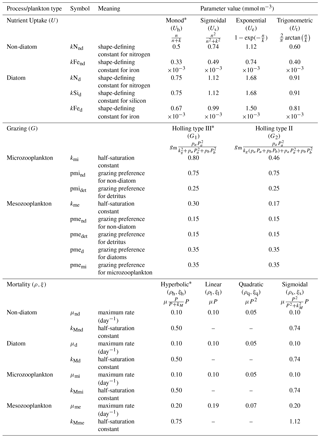
To explore structural uncertainty we first make the functional forms representing key processes more similar to each other by tuning the shape-defining parameters. For example, for Holling type II and Holling type III, we fix the maximum rates of each process and implement a non-linear least-squares method to optimize the half-saturation coefficients so that the overall shapes are similar. This approach is used for nutrient uptake (four functional forms), phytoplankton mortality (four functional forms), and zooplankton mortality (four functional forms), as in the subsections below. Table 1 shows the equations and parameter values.

2.1 Nutrient uptake

Alongside light, nutrient concentration limits the growth of phytoplankton. In MEDUSA the standard hyperbolic Monod, hereafter U_h, function is the default. The growth of cells monotonically increases with ambient nutrient concentration and halts when nutrients become scarce. If nutrient concentrations are high, the rate of uptake saturates. Other mathematical functions show similar properties including (i) sigmoidal (Fennel and Neumann, 2014), U_s; (ii) the exponential (Ivlev, 1961), U_e; and (iii) trigonometric functions (Jassby and Platt, 1976), U_t. All these functions include a shape-defining parameter, k, which for Monod and sigmoidal can be interpreted as a half-saturation constant, and a maximum uptake rate, $V_{p^T}$, which is a function of temperature (Eppley, 1972): $V_{p^T}=V_p{\mathrm{1.066}}^T$, where V_p is the maximum growth rate when temperature, T, is at 0 ^∘C. The uptake functions of different phytoplankton types and nutrients use similar functions but different parameter values for k, summarized in Table 1, obtained by minimizing the sum of the squared difference with U_h. The nutrient uptake functions after optimization are shown in Fig. 1a. The fit is done over the nutrient concentration ranging from 0.001 to 20 mmol N m⁻³ and are discretized into 1000 intervals. The differences in shape of the optimized functional forms are more obvious between 0.1 and 1 mmol N m⁻³. The fitting was done based on the non-linear least-squares optimization method using Python's curve_fit function from scipy.optimise.

2.2 Zooplankton grazing

In MEDUSA, both phytoplankton and zooplankton are grouped into “small” and “large” categories. The small zooplankton, represented by the microzooplankton, graze on non-diatoms and detritus, with the more nutrient-rich, higher-quality non-diatoms preferred over detritus. Larger zooplankton, represented by mesozooplankton have a broader range of prey, including both microzooplankton and diatoms, which are higher-quality food sources compared to non-diatoms and detritus. When describing multiple grazing functions, the zooplankton grazing rate is often defined using either the Holling type II (hereafter G₂) or Holling type III (hereafter G₁) function with maximum grazing rate g_m and a weighted preference on the different food sources p_n (Fasham et al., 1990). The preference parameter changes through the year as a function of the food ratio. G₂ and G₁ grazing on prey P_a are described in Table 1. In MEDUSA, the default multiple grazing parameterization is based on the sigmoid Holling type III (Ryabchenko et al., 1997) function. Apart from the weighted preference, both of these functions include a half-saturation constant k_x, where x is the zooplankton type.

These functions approach a maximum grazing rate at high concentrations of prey. During the fitting process, the range of phytoplankton and microzooplankton concentration used was 0.001 to 10 mmol m⁻³ and discretized in 1000 intervals. At low zooplankton concentrations the sigmoidal response has lower grazing rates than the hyperbolic, and therefore the sigmoidal curve has a more rapid increase in predation rate before becoming saturated (Edwards and Yool, 2000), shown in Fig. 1c. Preferences for food types are kept the same as MEDUSA's default parameters, with terms summarized in Table 1.

2.3 Plankton mortality

MEDUSA has both density-independent and density-dependent mortality rates for all the phytoplankton and zooplankton types. Density-independent loss is modelled by a linear function representing plankton metabolic loss, which was kept unchanged. Density-dependent loss includes processes such as higher trophic grazing and disease. In MEDUSA these processes are modelled using the hyperbolic function of plankton concentration (Fasham et al., 1993). Alternative functions can describe the density-dependent mortality, and we use the combinations of hyperbolic (ρ_h,ξ_h), linear (ρ_l,ξ_l), quadratic (ρ_q,ξ_q), and sigmoidal (ρ_s,ξ_s) functions to describe the phytoplankton (ρ) and zooplankton (ξ) mortalities (equations and abbreviations are shown in Table 1). Similar to grazing and nutrient uptake, the functional forms have different maximum rates for each plankton type. These maximum rates are made the same for all the different functions.

Of the four different mortality functions, linear and quadratic functions are most different in shape, as shown in Fig. 1c. Using the linear term is similar to a change in the value of maximum mortality rate, μ. To make the linear function similar to the sigmoidal and hyperbolic functions, the maximum mortality rate is set so that the total loss integrated over the range of phytoplankton concentrations (calculated as the area below the function representing the total loss in linear terms, between 0.001 and 10 mmol m⁻³) is similar to that for the hyperbolic curve. The quadratic term, instead of asymptoting, continues to grow with plankton abundance. In order to keep this similar to other forms, after reaching a certain concentration the function is switched to linear, so that the rate plateaus at high abundance. For sigmoidal mortality, the default μ's are not changed but the half-saturation constant, k_M, is optimized. The optimized mortality functions are shown in Fig. 1c. The range of phytoplankton and zooplankton concentrations used during the fitting process was between 0.001 and 10 mmol m⁻³ and discretized within 1000 intervals. A distinctive feature of these functional forms after optimization is that the quadratic mortality rate remains low until phytoplankton concentration reaches 1.0 mmol m⁻³, and the linear function shows consistently high plankton mortality (Fig. 1c).

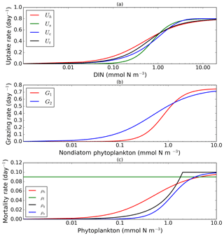
Figure 1 Nearly identical curves which describe resource uptake (a), zooplankton grazing (b), and phytoplankton mortality (c). Panel (a) shows four uptake functions, which have been optimized to the default uptake function, Monod (U_h). Panel (b) shows two grazing functional forms, the Holling type III (G₁) and type II (G₂) functions. Four phytoplankton mortality functions are shown in (c), whereby hyperbolic is the default function. The optimization method is described in Sect. 2.1, 2.2, and 2.3. The range for DIN in (a) is between 0.001 and 20 mmol m⁻³, and phytoplankton in (b) and (c) are 0.001 and 10 mmol m⁻³. Table 1 describes the function's equations and parameters.

Table 1 Parameter values for resource uptake (U), zooplankton grazing (G), and plankton mortalities (ρ and ξ for phytoplankton and zooplankton respectively), described using similar functional forms (shown in Fig. 1). In the grazing equation, g_m represents the maximum grazing rate, P_a is the prey, and p_a denotes the grazing preference. Starred equations are the default functional responses in MEDUSA.

2.4 Model parameters

Apart from sinking rate, maximum growth, and grazing rates, parameters not listed in Table 1 are kept at their default values (Yool et al., 2011 shown in Tables 1–4). From a previous 3-D MEDUSA run, the oligotrophic regions show a low “background” chlorophyll concentration (Yool et al., 2011) so to raise this concentration a higher maximum growth rate and lower grazing rate have been used. The maximum uptake rate, V_p, is 0.8 day⁻¹, similar to that in the HadOCC model (Palmer and Totterdell, 2001). For zooplankton grazing, similar to NPZ models (Anderson et al., 2015; Fasham, 1995; Fasham et al., 1990), we use 1 day⁻¹ as the maximum grazing rate, g_m. MEDUSA also parameterizes both slow and fast detritus sinking factors. It is assumed that the latter sinks rapidly relative to the model time step, and remineralization of the detrital nitrogen and silicon is done implicitly. In the default model 3 m day⁻¹ is used for the slow sinking detritus; however over long runs we found this leads to downward loss of nutrients from the euphotic zone to the sea floor. Earlier studies have used lower detrital sinking rates (Fasham et al., 1990; Lacroix and Gregoire, 2002; Raick et al., 2006; Steele and Henderson, 1981), between 0 and 1.25 m day⁻¹, and other studies have suggested the use of 0 m day⁻¹ (Ward et al., 2013). We chose a sinking rate of 0.1 m day⁻¹, towards the lower end of the range of literature values to prevent depletion of state variables particularly at the shallower stations.

2.5 Running the model and generating the ensemble

MEDUSA is run in the Marine Model Optimization Testbed (MarMOT-1.1) (Hemmings and Challenor, 2012; Hemmings et al., 2015), a site-based mechanistic emulator, where simulations are run in 1-D. MarMOT was developed to investigate the effect of sensitivity in plankton model simulations, especially in regard to parameter and environmental inputs (Hemmings and Challenor, 2012). Despite some uncertainties associated with the differences in physical forcing, fluxes, and initial values of biogeochemical properties, using 1-D simulations to approximate 3-D model behaviour for calibrating models based on specific sites has improved the predictive skill of 3-D models (Kane et al., 2011; McDonald et al., 2012; Oschlies and Garçon, 1999; Oschlies and Schartau, 2005). The 1-D MEDUSA is run at five oceanographic stations: Porcupine Abyssal Plain Sustained Observatory (PAP-SO, hereafter PAP), A Long-Term Oligotrophic Habitat Assessment (ALOHA), Bermuda Atlantic Time Series (BATS), Cariaco, and L4 shown in Fig. 2. These are chosen as they represent different oceanographic regimes: abyssal plain (PAP), oligotrophic (ALOHA, BATS), and coastal (Cariaco, L4).

At each oceanographic station, all combinations of the optimized functional forms (as described in Sect. 2.1, 2.2, and 2.3) are then embedded into the 1-D MEDUSA code. The same process function is always used for both diatoms and non-diatoms, or mesozooplankton and microzooplankton. Each ensemble member has at least one functional form changed from the default functions. This provides a total number of 128 combinations, arising from four types of nutrient uptake, four phytoplankton mortality formulations, two types of zooplankton grazing, and four zooplankton mortalities. The model ensemble at each station is initialized using in situ measurements of chlorophyll, inorganic nitrogen, silicic acid, and iron, and the ensemble is run over 10 years starting from January 1998.

2.5.1 Physical input

Physical input files consist of gridded values of vertical velocity (m day⁻¹), vertical diffusion coefficient (m² day⁻¹), and temperature (^∘C), which are applied at each depth level. Additionally, time series of downwelling solar radiation (W m⁻²) and mixed layer depth (m) are also used as input. These are obtained from the 5-day mean output of the Nucleus for European Modelling of the Ocean (NEMO) model, using the Met Office Forecast Ocean Assimilation Model (FOAM), which controls the physical parameters and therefore the biogeochemical tracers every 5 days. The FOAM–NEMO system assimilates satellite-derived sea surface temperature, sea-level anomaly, sea-ice concentration, temperature, and salinity profile data, in order to make the physical system more realistic (Storkey et al., 2010). However, assimilating physical data directly into a coupled physical–biogeochemical model often does not improve the simulation of the ecosystem. For example when assimilation is used in the 3-D HadOCC model it overestimates the nutrient concentrations due to spurious vertical velocities (Ford et al., 2012; Ourmières et al., 2009).

To avoid overestimating surface nutrients the vertical velocities from the FOAM system were capped at the 90th and 10th quantiles, and the 10-year mean of the vertical velocity is also removed. This means that the time mean of vertical velocity is zero. These adjustments gave a better long-term vertical structure to the nutrient and other distributions. Since input data on the vertical diffusivity were not stored in FOAM, we used values from the NEMO ORCA025-N102 output from January 1998 to December 2001 and from ORCA0083-N01 from January 2002 to December 2007, both obtained from the CEDA Group workspace web (http://gws-access.ceda.ac.uk/public/nemo/#_top, last access: 29 September 2016). These physical inputs are 5-day averaged and are available at 75 depth levels (from 0.5 to 6000 m) for NEMO–FOAM and ORCA0083-N01 and at 63 depth levels (spanning from 6 to 5800 m) for NEMO ORCA024-N102, with less depth intervals than the 75 levels. The level thickness increases exponentially as the depth goes deeper. Our 1-D model uses these same 63-depth-level thicknesses of vertical resolution in order to minimize computational costs.

2.5.2 Biogeochemical input and validation data

The 1-D MEDUSA ensemble is run at five oceanographic stations: PAP, ALOHA, BATS, Cariaco, and L4. The inputs for the biogeochemical environment are the initial conditions for the 11 primary tracers (state variables) including dissolved organic nitrogen (DIN), non-diatom, diatom, silicon in diatom, silica, detritus, microzooplankton, mesozooplankton, non-diatom chlorophyll, diatom chlorophyll, and iron (mmol m⁻³), along with the model parameter values. Initial conditions for chlorophyll, silicate, iron, and DIN concentrations are taken from the in situ data at the five oceanographic stations. We did not use spin-up runs when initializing, as discussed in Sect. S1 in the Supplement. Location coordinate, data source, and maximum depth are summarized in Table 2 and the stations locations are shown in Fig. 2. After initialization, in situ data from these stations are used to validate the model results. For station PAP, we also use SeaWIFS-derived chlorophyll a data with 9 km spatial resolution and 8-day averages provided by GlobColor (http://hermes.acri.fr/, last access: 10 July 2017) for validating the surface chlorophyll.

Table 2 Location, data source, and available depth range for the five oceanographic stations.

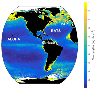
Figure 2 SeaWIFS-derived mean 1998 chlorophyll a (mg m⁻³) overlain with the five oceanographic stations (red dots). These stations are located in different oceanic regions: oligotrophic (ALOHA and BATS), coastal (L4 and Cariaco), and abyssal plain (PAP).

At these stations, the DIN consists of ammonia, nitrate, and nitrite; however at oligotrophic stations like ALOHA the ammonium is below the detection limit (Hawaii Ocean Time Series, 2018), and therefore DIN only consists of nitrate and nitrite. At PAP we use the initial condition from one of MarMOT's test stations, located at 50^∘ N, 20^∘ W (Hemmings et al., 2015), since the nitrate data were only collected between 30 and 400 m. At station L4 chlorophyll and DIN data were collected from the surface from 1999 to 2008. Since the maximum depth in this station is only 50 m, the initial concentrations for chlorophyll and DIN are the same at every depth (total chlorophyll = 0.27 mg m⁻³, DIN = 6 mmol m⁻³). Other inputs that are not available at the websites mentioned above, such as microzooplankton, mesozooplankton, and detritus, were taken from the nearest test stations. In the oligotrophic stations, 75 % of total chlorophyll was allocated initially to the non-diatom phytoplankton since these dominated the water column (Villareal et al., 2012). At the other stations half of the total chlorophyll goes into the diatoms.

For validation of the model, we consider the total chlorophyll a concentration, instead of separating diatoms and non-diatoms. The model is simulated at 37 depth levels, spanning from 6 to 1200 m instead of from 6 to 5800 m to minimize computational cost, apart from station L4, with a maximum depth of 50 m, and Cariaco, where the maximum depth for the physical input is available down to 500 m, although the depth at which nutrients are sampled is down to 1310 m. The boundaries for the depth levels are as follows: 6, 12, 19, 25, 32, 39, 46, 54, 62, 71, 80, 90, 100, 112, 124, 137, 152, 168, 187, 207, 229, 254, 281, 312, 347, 386, 429, 477, 531, 591, 656, 729, 809, 896, 991, 1093, and 1200 m. At the lowest level, vertical velocity and diffusion are set to zero and this level is a sink for detritus. Stations that have shallower maximum depths are run with fewer depth levels. Additionally, apart from the physical input files a time series for soluble iron flux from dust deposition is applied, but this is constant using the average value from Mahowald et al. (2009).

2.6 Model metrics

We use statistical metrics including correlation coefficient, root-mean-squared error, bias, ensemble range, and 10-year mean depth profiles of DIN and chlorophyll and integrated chlorophyll in order to compare the ensemble model with the default model and how well it represent the observations. For surface chlorophyll, apart from the metrics above we use the mean chlorophyll abundance each year in order to see inter-annual variability, as well as monthly abundance for the seasonal variations. A similar approach is applied to DIN; however we use the averaged DIN over 200 m (integrated DIN / depth) to calculate the inter-annual mean and monthly abundance. These statistical metrics are compared with in situ data. We also consider the phenological aspects of the phytoplankton spring bloom, which are useful ecological indicators for detecting natural and anthropogenic impacts on the pelagic ecosystem (Platt and Sathyendranath, 2008). We consider seven phenology indicators as metrics, including an initiation time where the chlorophyll concentration exceeds a certain threshold, at half the concentration of the bloom peak. When the bloom concentration starts to diminish, we derived a termination time, where bloom concentration falls below the same threshold. The number of days when chlorophyll concentration is higher than the threshold is the bloom duration. The concentration at the bloom peak and the date it takes place are also included as indicators. We also note the amplitude of the bloom, which is half of the peak height minus the minimum chlorophyll concentration. These indicators are derived using the method described in Appendix A and applied to all ensemble outputs for each year.

In an ensemble forecast system, an ensemble with good reliability is the one that is statistically consistent with the observations, such that the observation is statistically indistinguishable from the ensemble members. In order to assess the value of the ensemble probability distribution we must assess the consistency of the ensemble spread as well as the ensemble mean error (Moradkhani and Meskele, 2010). A simple method is discussed by Anderson (2001) that takes the ratio R_a of RMSE of the ensemble mean and the mean RMSE of all the ensemble members, which has the expectation value $E\left[R_a\right]=\sqrt{\frac{(n+\mathrm{1})}{\mathrm{2}n}}$, where n is the number of ensemble members. This is called the normalized RMSE ratio (NRR = R_a∕E[R_a]), where the desirable ensemble spread is expected to have NRR=1. If the NRR>1 then the spread is too small, and NRR<1 indicates that the ensemble spread is too large. We may expect different NRR values for different metrics and also for variability on different timescales, such as monthly or inter-annual data. This method has previously been used to set the number of ensemble members in data assimilation (Moradkhani et al., 2006; Roy et al., 2012).

3 Results

In this section, the ensemble mean and median, spread (NRR), and range are compared with the observations. Inter-annual and monthly variabilities are considered, and both biological concentrations and phytoplankton bloom phenology are assessed. The abyssal plain station comparisons are discussed in Sect. 3.1, followed by the two oligotrophic stations (Sect. 3.2) and the two coastal stations (Sect. 3.3).

Table 3 Error statistics, 10-year mean, and NRR of chlorophyll (mg m⁻³) and DIN (mmol m⁻³) concentration at five stations for the default run, ensemble mean, ensemble median, and the ensemble range (ensemble maximum minus ensemble minimum). These are calculated from surface to 200 m depth, starting from January 1998 to December 2007. Bias is (model output) − (in situ observation). Bold text indicates the smallest RMSE. At station L4 error statistics and mean are taken from the surface and start from January 1999 for chlorophyll and June 2000 for DIN. For station PAP, error statistics are taken from 2002 to 2004 since in situ data are only available during that time.

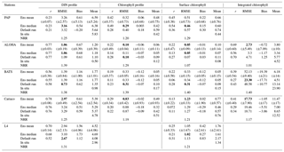
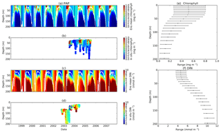
Figure 3 Chlorophyll and DIN profiles from ensemble mean (a and c respectively), in situ observations (b and d for chlorophyll and DIN respectively), and the 75th and 25th quartile range of concentrations at each depth (e for chlorophyll and f for DIN) at station PAP. The ranges are obtained by averaging the concentrations from all ensemble members for 10 years at each depth. The black dots in the second column show the mean concentration of the ensemble mean over the time series (from January 1998 to December 2007). The white solid line in (a) and (c) show mixed layer depth.

3.1 Abyssal plain

The abyssal plain is represented by station PAP located in the North Atlantic. However in situ sampling is limited, with nitrate only measured from mid-2002 to mid-2004 and to a maximum depth of 400 m and chlorophyll from mid-2003 to mid-2005 with a maximum depth of 200 m, as in Table 2. Surface chlorophyll is derived from SeaWIFS (8-day averages) and is available for the full 10-year time series (see Fig. S5 in the Supplement).

The PAP data show seasonality in both chlorophyll and DIN concentrations, with high DIN during winter (December–April) and a decline in summer (Fig. 3b). The averaged DIN profile peaks in February, with a spike of high DIN in September, as shown in Fig. 7a. At around 70 m the highest concentrations of chlorophyll occur in May–June, summarized in Fig. 3b, similar to that in the surface. An inter-annual decline has been observed in the satellite-derived chlorophyll ($r=-\mathrm{0.21}$, p<0.05), shown in Fig. 4a.

The ensemble mean reproduces the seasonality in averaged DIN in Fig. 7a, but with later peak concentrations in March and April, compared to in situ, and with a secondary peak in July instead of September. The ensemble mean chlorophyll also has a seasonal cycle but with chlorophyll confined to shallower depths than in situ, summarized in Fig. 3a and e. The ensemble mean chlorophyll starts to decline below 50 m, which also corresponds to the decline in the chlorophyll interquartile (between the 25th and 75th percentile) range with depth, shown in Fig. 3e. At the surface, the ensemble peak chlorophyll occurs in May, similar to in situ, although peak concentrations are higher than in situ. The decline in surface chlorophyll in the observation has been captured by six ensemble members (U_tρ_hξ_hG₂, U_tρ_hξ_sG₂, U_tρ_lξ_qG₂, U_tρ_qξ_lG₂, U_tρ_qξ_qG₂, and U_tρ_sξ_lG₂), although with weaker correlations ($r=-\mathrm{0.14}$ (±0.06), p<0.05).

In situ chlorophyll and DIN vertical profile means fall within the ensemble range, with NRR=1.20 and 1.25 for chlorophyll and DIN respectively. For both the surface and upper layer chlorophyll the ensemble median is better than the default model, showing a higher correlation, a lower RMSE, and lower bias, against the in situ and satellite-derived chlorophyll values (Table 3). The highest chlorophyll profile RMSEs (>0.62 mg m⁻³) are produced from ensemble members that combine G₁ with ρ_hξ_l, ρ_qξ_q, and ρ_hξ_s, and this also coincides with high chlorophyll profile concentrations (>0.7 mg m⁻³). However for DIN the ensemble mean and median RMSEs are higher than in other regions, which is traced to have been due to ensemble members that contain the U_tG₂ combination which has a particularly high DIN bias (>9 mmol m⁻³), as shown in Fig. 13j.

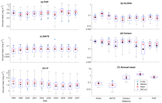
Figure 4 Inter-annual mean of surface chlorophyll from all the study sites (a–e) and the 10-year annual mean (f), all measured in mg m⁻³. The box plots show the ensemble annual means. The blue cross is the in situ observation; the red open circle, black dot, and blue stars are the ensemble mean, median, and the default run respectively. The blue box is the 75th and 25th quartiles. The red line is the median. The whiskers are the ensemble minimum and maximum mean of surface chlorophyll. Annual mean values and NRR are described in Table 4.

At the surface, in years 1998, 1999, and 2001, the satellite-derived chlorophyll is within the interquartile range; however, in other years, it is well below the ensemble interquartile box limits (Fig. 4a). The ensemble spread for inter-annual means has an NRR of 1.26, and there is also an effect on the overall 10-year ensemble spread (see Fig. S5) with an NRR of 1.29. High surface chlorophyll concentrations with high RMSE (>0.8 mg m⁻³) are seen when combining U_h with ρ_hξ_l, ρ_qξ_q, and ρ_hξ_s, see Fig. 12e and j, which is consistent with the largest errors in the profile average values. However the low chlorophyll concentrations (<0.4 mg m⁻³) that are produced when combining U_t and G₂ in the profile averages are not reproduced in the surface chlorophyll.

The ensemble range of surface chlorophyll annual mean is 0.7 mg m⁻³. However if we only allow one process function to change in each ensemble member, keeping the other processes with their default functions, the new 11-member ensemble range reduces to 0.58 mg m⁻³, still covering 83 % of the full ensemble (128 members). When the original MEDUSA parameters are used, the ensemble fits the inter-annual surface chlorophyll observations slightly better, but the DIN fit gets worse. The results from using the original MEDUSA parameters (maximum growth and grazing rates) and including in situ DIN concentrations as initial conditions can be found in Sects. S2 and S3.

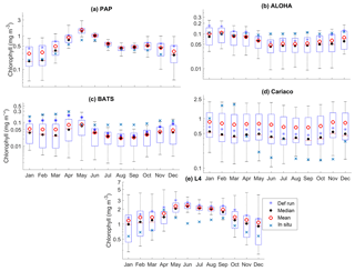
Figure 5 The 10-year monthly mean surface chlorophyll from all the study sites (a–e), showing the seasonal dynamics of surface chlorophyll (mg m⁻³). The box plots show the ensemble seasonal means. The blue cross is the in situ observation; the red open circle, black dot, and blue stars are the ensemble mean, median, and the default run respectively. The blue box is the 75th and 25th quartiles. The red line is the median. The whiskers are the ensemble minimum and maximum mean of surface chlorophyll. In station PAP, in situ data for December are not available due to low light and high cloud cover.

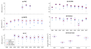
Figure 6 Inter-annual variability of DIN averaged over 200 m, from all the study sites (a–e) and the annual mean (f). Since the in situ data for PAP do not always cover the first 200 m, the overall mean DIN concentration from all depths is used instead. For station L4, in situ DIN is only collected on the surface. The blue cross is the in situ observation; the red open circle, black dot, and blue stars are the ensemble mean, median, and default run respectively. The blue box is the 75th and 25th quartiles. The red line is the median, and the whiskers are the ensemble minimum and maximum of the averaged DIN. In station L4 and PAP data for DIN are only available from 2000 to 2007 and from 2002 to 2004 respectively.

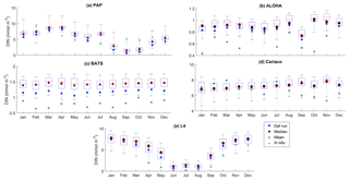
Figure 7 The 10-year monthly mean of DIN averaged over 200 m from all the study sites (a–e), showing the seasonal dynamics of DIN (mmol m⁻³). For station PAP, the DIN shown is the overall profile, and in L4 the in situ DIN concentration is only available at the surface. The box plot shows the ensemble monthly means. The blue cross is the in situ observation; the red open circle, black dot, and blue stars are the ensemble mean, median, and the default run respectively. The blue box is the 75th and 25th quartiles. The red line is the median. The whiskers are the ensemble minimum and maximum mean of averaged DIN. In station PAP, the in situ data are only collected from 2002 to 2004 and L4 from 2000 to 2007.

Table 4 Surface annual mean and phytoplankton phenology from the in situ, ensemble mean, median, and default run. The ranges and NRR in the brackets are the values for changing the functional form one process at a time (shown in Fig. 8).

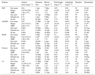
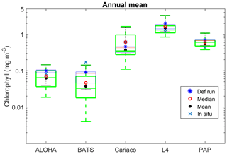
Figure 8 Annual mean of surface chlorophyll when changing only one process at a time (blue box), overlain with annual mean of all ensemble members (green box) at five oceanographic stations. Ensemble mean and median plotted in the figure (shown in red open circles and black closed circles) are the from the 128 ensemble members.

3.2 Oligotrophic ocean

The oligotrophic region is represented at stations ALOHA and BATS. The nutrients in this region are scarce at the surface but may be plentiful at deeper depths (Dave and Lozier, 2010; Lipschultz, 2001). High DIN levels (>1.0 mmol m⁻³) are only found below ∼150 m depth, shown in Fig. 9d and j for ALOHA and BATS respectively. The annual means of the averaged DIN profile in the top 200 m are 0.68 and 0.80 mmol m⁻³ for ALOHA and BATS respectively. In station ALOHA, an increasing trend of the inter-annual in situ averaged DIN profile (r=0.69, p<0.03) has been observed, shown in Fig. 6b. In the oligotrophic region, seasonality has not been observed in both chlorophyll and DIN. However, there are months of low chlorophyll (<0.1 mg m⁻³) that have been observed in July–October, as shown in Fig. 5b and c. Another feature of the oligotrophic ocean is a deep chlorophyll maximum (DCM) that occurs below the mixed layer, when the chlorophyll concentration in the surface is low (Fennel and Boss, 2003; Letelier et al., 2004). At both stations, the DCM is observed between 70 and 150 m depth and continuously occurs throughout the year.

The ensemble mean has reproduced the DIN concentration distribution in station ALOHA as seen in Fig. 9c and d. The ensemble range decreases as the depth increases, with a high ensemble range found at depths between 3 and 50 m (Fig. 9f and l). However, at BATS, the DIN concentration in the top 200 m (Fig. 9i) is higher (>1.0 mmol m⁻³) at ∼10 m. This consequently leads to a higher annual mean of >1 mmol m⁻³ and an overestimation of monthly (Fig. 7c) and inter-annual variability (Fig. 6c) of the averaged DIN profile, for all the ensemble members. This higher averaged DIN profile concentration has also been observed at ALOHA, whereby both the ensemble mean and median have annual means of >0.9 mmol m⁻³. The increasing trend in DIN (r=0.67, p< 0.03) has also been observed in 28.9 % of the ensemble members, which uses G₂ as its grazing function.

DCM has also been observed at both stations in the ensemble mean. However, the depths at which the DCM is simulated are slightly shallower, between 70 and 90 m in BATS and between 70 and 150 m in ALOHA. None of these stations show continuous DCM, shown in Fig. 9a and g for ALOHA and BATS respectively. The depth of the DCM coincides with the higher ensemble range, with the range decreasing with depth after the DCM depth. At the surface during months with high chlorophyll (>1 mg m⁻³), the in situ concentrations are within the interquartile range box shown in Fig. 5b and c. Although during months of low concentration most of the ensemble means show even lower chlorophyll (as low as 0.045 and 0.022 mg m⁻³ for ALOHA and BATS respectively).

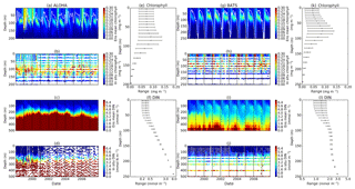
Figure 9 Time series (from January 1998 to December 2007) of ensemble mean and in situ concentrations, and range of chlorophyll and DIN at oligotrophic stations. Station ALOHA is shown in (a)–(f) and BATS is shown in (g)–(l). The white solid line in (a) and (g) represents mixed layer depth. (e), (f), (k), and (l) are the 75th and 25th percentile range of chlorophyll (e for ALOHA and k for BATS) and DIN (f for ALOHA and l BATS) over the depth. The range is obtained by averaging the chlorophyll and DIN concentrations of each ensemble member over the time series at each depth. The black dots in (e), (f), (k), and (l) are the mean of the ensemble. Ensemble mean chlorophyll profiles (shown in a and g) and DIN (c and l) are obtained from all of the ensemble members. In situ chlorophyll is shown in (b) and (h), and DIN is shown in (d) and (j), for ALOHA and BATS respectively.

Figure 10 Mean integrated primary production averaged over 200 m that is available in (a) ALOHA and (b) Cariaco, and (c) the annual mean. The NRRs for ALOHA and Cariaco are 1.12 and 0.80 respectively.

The DIN concentrations at both oligotrophic stations are mostly overestimated by the ensemble mean and median, and the opposite has been observed in chlorophyll. At BATS all of the ensemble members overestimate the chlorophyll profile, surface, and integrated. From Fig. 11a and b, low chlorophyll profile means (<0.08 mg m⁻³) are produced from ensemble members that combine G₂ with ρ_lξ_l, ρ_lξ_q, ρ_lξ_s, ρ_qξ_h, and U_e, which coincides with high RMSE, shown in Fig. 11e and f. The default run has lower RMSEs than the ensemble mean and median, summarized in Table 3. High chlorophyll vertical profile means at both stations are produced from ensemble members that combine U_hG₁ and U_tG₁. High DIN profile means are produced when U_e and U_s are combined with any mortality function, summarized in Fig. 13a and b. Combining these uptake functions with G₂ will also increases the mean DIN concentration even further and therefore increase the RMSE in station BATS. Nevertheless, since overestimation of mean DIN concentration occurs in most of the ensemble members, and therefore the ensemble mean, the NRRs are high for both ALOHA and BATS (NRR=1.38 and 1.40 respectively).

At station ALOHA, surface chlorophyll (Fig. S2) RMSEs from the ensemble mean and median are lower compared to the chlorophyll profile. The surface mean concentrations from the ensemble mean and median are also closer to the in situ concentration, summarized in Table 3. Ensemble members with low surface chlorophyll means are consistent with the profile averaged values, although high surface chlorophyll errors also coincide with high surface mean, summarized in Fig. 12a and f. The low RMSEs for surface chlorophyll at ALOHA are also reflected in the NRR (1.07), and the ensemble almost always encompasses the in situ observations (see Fig. S2). The default run in oligotrophic regions generally produces higher chlorophyll and lower DIN concentrations compared to the ensemble mean and median. The default run also matches better with in situ data as the correlation coefficient, r, is higher. Nevertheless, the ensemble mean and median at ALOHA also have lower bias and RMSE for surface chlorophyll compared to the default. However, at BATS the default run shows better RMSE and bias. For integrated chlorophyll in the oligotrophic region, the ensemble mean and median have smaller RMSEs and a better correlation coefficient, compared to the default run. The NRR for the integrated chlorophyll is closer to 1 compared to the surface and chlorophyll profiles.

At ALOHA the range for inter-annual means has low NRR (0.84), which is lower than the overall time series mean. However, if we only allow one process function to change in each ensemble member, whilst keeping the other processes with their default function, the new ensemble produces higher NRR (1.17), and the in situ annual mean is no longer within the interquartile range, as shown in Fig. 8 and summarized in Table 4.

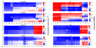
Figure 11 Chlorophyll profile 10-year means (a–d) and its RMSEs (e–h) at four oceanographic stations from all of the ensemble members. Station L4 is not included as chlorophyll data are only taken at the surface. These are arranged from the lowest chlorophyll mean to the highest, depending on the oceanographic regions.

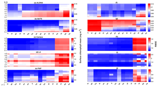
Figure 12 The 10-year mean and RMSE of surface chlorophyll (mg m⁻³) at five stations from all ensemble members. The first column (panels a–e) shows surface chlorophyll mean and RMSEs are shown in the second column (panels f–j). Concentrations and RMSEs in each panel are arranged from the lowest chlorophyll mean to the highest, depending on the oceanographic regions. For station PAP, the sequence is sorted based on coastal station. The y axis shows combinations of uptake (U_h, U_s, U_e, and U_t) and grazing (G₁ and G₂), and the x axis shows combinations of phytoplankton (ρ) and zooplankton (ξ) mortalities.

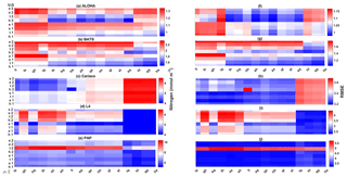
Figure 13 The 10-year mean and RMSE of DIN (mmol m⁻³), at five stations from all ensemble members. The first column (panels a–e) shows the DIN mean and RMSEs are shown in the second column (panels f–j). Concentrations and RMSEs are arranged from the lowest DIN mean to the highest, depending on the oceanographic regions. For station PAP, the sequence is sorted based on coastal station. The y axis shows combinations of uptake (U_h, U_s, U_e, and U_t) and grazing (G₁ and G₂), and the x axis shows combinations of phytoplankton (ρ) and zooplankton (ξ) mortalities.

3.3 Coastal

Coastal zones are represented by stations Cariaco and L4, with in situ observations showing strong seasonality, in Fig. 14b, d, g, and h. At Cariaco, the highest mean DIN profile concentration (>7.5 mmol m⁻³) at the top 200 m is observed in March and July and the lowest (<5.5 mmol m⁻³) in November (see Fig. 7d). At L4 high concentrations (>8 mmol m⁻³) are observed between November and February, with very low values (∼0.1 mmol m⁻³) during summer months (Smyth et al., 2010). The in situ profiles at Cariaco show high chlorophyll concentrations (>1 mg m⁻³) within the upper 30 m between December and February (see Fig. 14b), coinciding with the rise in nitrogen from depth to ∼30 m, seen in Fig. 14d, increasing the nitrogen concentration to ∼5 from <1 mmol m⁻³. Similarly at L4, Fig. 14g, sharp peaks of chlorophyll are observed during spring (March–April) and fall (September), coinciding with the sharp decline of DIN between April and July (from ∼6 in March to 0.22 mmol m⁻³ in July), shown in Fig. 7e, resulting in an annual mean of 2.40 mmol m⁻³ and 1.20 mg m⁻³ for DIN and chlorophyll respectively. During non-bloom periods, chlorophyll is observed from 0.09 to 2 mg m⁻³, with peak concentrations up to 6.4 mg m⁻³.

At Cariaco seasonal variability is absent from the ensemble for both chlorophyll and DIN. There are only 2 years simulating downwelling of DIN, in 2001 and between 2005 and 2006, shown in Fig. 14c. The chlorophyll concentration is almost constant (above 0.7 mg m⁻³) in the upper 30 m and at the surface (Fig. S3), apart from a decline in concentration to ∼0.5 mg m⁻³, followed by a sharp chlorophyll peak in the winter (December–January) in 2007, shown in Fig. 5d. A decline of chlorophyll was noted at Cariaco from 2004 (Taylor et al., 2012), and this is captured by the ensemble mean, median, and the default ($r=-\mathrm{0.72}$, p<0.05, $r=-\mathrm{0.66}$, p<0.05, and $r=-\mathrm{0.35}$, p<0.05 respectively).

At L4 the ensemble shows seasonality, although the interquartile range often overestimates the surface DIN concentrations, especially during the sharp decline in spring and summer, shown in Fig. 7e. The two bloom events per year in the observations are not represented and the ensemble only simulates one peak between May and June, summarized in Fig. 7e. However if only the diatom chlorophyll concentration is shown, the two bloom events are captured, especially in the default run (see Fig. S4). The ensemble also shows a higher concentration range during non-bloom periods (ensemble range from 0.28 to 3.13 mg m⁻³), so that the surface chlorophyll is not fully captured by the ensemble.

At Cariaco, although surface chlorophyll seasonality is not well reproduced, the ensemble range is wide so that in situ concentrations mostly fall within it, apart from August and November, summarized in Fig. 5d. The annual mean of surface chlorophyll and averaged DIN in the top 200 m are also within the ensemble range, Figs. 4f and 6f, with the NRR being 0.78 and 1.15 for chlorophyll and the averaged DIN profile respectively. At L4, despite reproducing seasonality, ensemble concentrations for DIN and chlorophyll are overestimated, and the NRR values for DIN and chlorophyll are 1.31 and 1.21 respectively, summarized in Table 3. At both stations, for the inter-annual mean, the ensemble range always encompasses the observations (Fig. 4c and d). Weak positive correlations and small RMSEs are found for ensemble mean surface chlorophyll at both stations, which are improvements over the default run. Similar to the oligotrophic stations, the integrated chlorophyll shows better correlation with in situ measurements, compared to both surface and chlorophyll profiles, with results summarized in Table 3.

The overestimation of DIN and chlorophyll is produced when the model uses ρ_lξ_q, ρ_hξ_l, ρ_qξ_q, and ρ_hξ_s combinations as these functional forms produced high chlorophyll means for both stations (>0.8 mg m⁻³ in the Cariaco profile and >1.5 mg m⁻³ in the L4 surface), with higher RMSEs, especially when U_s is also used. Higher DIN concentrations in Cariaco (>5 mmol m⁻³) with high RMSEs (>3.4 mmol m⁻³) are also associated with the same ensemble members, summarized in Fig. 13c. However at L4 these same ensemble members show relatively low DIN concentration (>5 mmol m⁻³) with lower RMSEs. From Table 3, at Cariaco, in situ surface chlorophyll concentrations are slightly overestimated by the ensemble mean but most other ensemble outputs are underestimated, except for ensemble members that use the combinations above. Unlike the oligotrophic regions, these high chlorophyll concentrations in the coastal stations coincide with a higher RMSE (>1.7 m⁻³).

Surface chlorophyll at these coastal stations also has a higher ensemble range than at other stations, summarized in Table 3. The Cariaco inter-annual mean chlorophyll (Fig. 4d and g) has an NRR of 0.78, indicating this wide ensemble spread. Inter-annual primary production also shows a wider spread compared to ALOHA, in Fig. 10b and c. However, if process functions are only perturbed one at a time the reduced ensemble has an NRR of 0.90, which is closer to the ideal ensemble range. At L4 the in situ annual mean of the full ensemble has an NRR of 1.00, with the in situ chlorophyll close to the ensemble median (see Fig. 4e). If the ensemble is reduced to single process perturbations the NRR increases to 1.36, and the in situ data are no longer within the ensemble range, shown in Fig. 8.

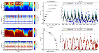
Figure 14 Time series of the chlorophyll and DIN profiles of the ensemble mean, their range, and in situ concentrations at the coastal stations Cariaco (a–f) and L4 (g–h) from January 1998 to December 2007. Panels (a) and (c) show the chlorophyll and DIN ensemble mean at Cariaco respectively. The white solid line in (a) is the mixed layer depth. Panels (e) and (f) show the 75th and 25th percentile of chlorophyll and DIN concentrations at each depth. The black dots are the mean of the ensemble. These ranges are obtained from the 10-year mean concentrations at each depth. Since in situ chlorophyll and DIN were taken at the surface in station L4, only surface time series were shown in (g)–(h). The grey shades on the chlorophyll, shown in (g), and DIN, shown in (h), time series show the 75th and 25th percentile of the range. The blue and red dots are in situ concentrations for chlorophyll and DIN respectively.

3.4 Phytoplankton phenology

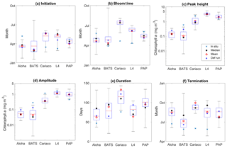
Figure 15 Phytoplankton phenology metrics at the five stations. The blue cross is the in situ observation; the red, black, and blue dots are the ensemble mean, median, and the default run respectively. The timings and concentrations are averaged annually from January 1998 to December 2007.

There are some relatively small differences in the timing of phenological events between the ensemble mean–median and the default run, ranging from a couple of days to a couple of weeks, as shown in Table 4. However the timing of initiation, bloom peak, and terminations show wide ensemble interquartile ranges for all stations and can lie between ∼20 and 100 days earlier than the in situ timing, apart from stations PAP and ALOHA (see Fig. 15b). For this reason at most stations the observed phenology metrics fall within the full ensemble range. The ensemble range also mostly encompasses the in situ peak and amplitudes, shown in Fig. 15c.

At station ALOHA, the observed initiation times show more inter-annual variability (Fig. S6) and may occur in June, August, and October, as well as in December and January. This causes the average observed initiation time to end up in May. The chlorophyll at ALOHA, Fig. 5b, shows peak highs (>0.1 mg m⁻³) in June, August, and September as well as December and January. At BATS, the initiation occurs mostly between January and February, although in 2002 the initiation occurred in October. Bloom peaks generally occur a month later, and the terminations vary between April and May, apart from 2002 when it was in December. The heights of the peak and amplitude at ALOHA are 0.14 and 0.05 mg m⁻³ respectively. At BATS these metrics have slightly higher chlorophyll concentrations of 0.60 and 0.28 mg m⁻³ for peak and amplitude respectively. The duration of the bloom at ALOHA is rather short compared to other stations, ∼50 days, whereas BATS is ∼90 days.

At ALOHA, Fig. 15a shows the ensemble run having initiation times between late January and April instead and so the observations fall outside the ensemble range (Fig. 15b) and the ensemble does not show as strong inter-annual variability as the observations (Fig. S6). The ensemble at BATS has the largest range of phenological timings, especially in termination time, and this matches the observations better. For bloom initiation, the in situ timing is within the interquartile range and only 3 days earlier than the ensemble median. However, since the earliest peak occurs in mid-January in the ensemble, the peak bloom time from the ensemble at BATS is usually later than in situ. Nonetheless, the ensemble estimates of bloom peaks for 30^∘ N agree with a study by Racault et al. (2012), who identify early April as the peak bloom time. Although the ensemble range of peak bloom time at BATS is high (174 days), the NRR is 1.17, as the ensemble does not cover all the in situ timings.

At ALOHA ensemble bloom peak and amplitude interquartile ranges encompass the observations, with ensemble mean and median being very close to the observation. However, at BATS, the in situ observations for peak and amplitude are outside the ensemble range, consistent with Sect. 3.2. The observed bloom duration at ALOHA and BATS is within the ensemble range, although the interquartile range at ALOHA shows longer bloom durations. For bloom termination, both stations show later termination, with the ensemble mean being almost 2 months late and a month late for ALOHA and BATS respectively. However, at ALOHA, located at 22^∘ N, the ensemble median for termination at the end of August agrees well with the observations from Racault et al. (2012).

For coastal stations L4 and Cariaco, the in situ initiation typically happens in mid-March, with peak bloom timing in April for both stations. At Cariaco the mean peak height is 3.5 mg m⁻³, with a mean amplitude of 1.15 mg m⁻³, shown in Fig. 15c and d. At L4, the mean peak height is slightly higher (3.6 mg m⁻³), with a higher amplitude (1.64 mg m⁻³). Both stations have nearly similar bloom duration, of 76 and 80 days for Cariaco and L4 respectively. This makes the termination times for both stations very similar, which happen in June.

The ensemble means show later initiation, with the 75th and 25th quartiles spanning mid-April to the end of May for Cariaco and between early and mid-May for L4. However, the overall ensemble range covers the observed initiation, in Fig. 15a. This later timing is also clear in peak bloom times for both stations, shown in Fig. 15b, whereby in L4 the interquartile range of the bloom occurs mostly in June and the ensemble range for Cariaco occurs between the end of May and early August. Consequently, the in situ observations for Cariaco and L4 both fall outside the ensemble range. Figure 5e shows that the bloom at L4 is simulated by the ensemble 1 to 2 months later. At Cariaco the ensemble peak height and amplitude reach less than half of the in situ values (mean = 1.10 mg m⁻³) and amplitude (mean = 0.38 mg m⁻³), which makes the in situ concentration fall outside the interquartile range for peak height and amplitude. This underestimate of the peak and bloom amplitude results in NRRs of 1.40 and 1.39 respectively. At L4, chlorophyll peaks are within the interquartile range, and amplitudes are within the full ensemble range. The bloom duration at Cariaco is also overestimated (up to 143 bloom days) and this, along with the late initiation of the bloom, results in a 3-month-late termination. Cariaco is the only station with peak bloom time, duration, and termination outside the ensemble range, due to the lack of chlorophyll seasonality, as noted in Sect. 3.3, also resulting in higher NRR values. At L4 the duration of the bloom is within the ensemble range; however, since the initiation and bloom timing of the interquartile range is later than the observation, the interquartile range also shows a later termination time.

At station PAP, the initiation from the satellite-derived chlorophyll occurs in April (see Fig. 15a). Although typical North Atlantic blooms happen in spring (Raymont, 1980), most peak blooms at PAP occur in late May–early June, as shown in Table 4 and Fig. 5. Additionally, a late bloom in September from satellite-derived chlorophyll occurred in 2005, making the mean bloom timing fall in June. The peak height is observed to be 1.52 mg m⁻³ with an amplitude of 0.45 mg m⁻³. The duration of the bloom is around 3 months (95 days), putting the mean termination in July.

The observed initiation time at PAP is within the ensemble interquartile range, and the ensemble median is only 1 week earlier than the observations. However, due to the inter-annual variability, the observed bloom peaks occur about a month later than the ensemble mean and median, although the bloom timing is still within the ensemble range, with an NRR value of 1.31. The ensemble mean produced higher peak chlorophyll (2.03 mg m⁻³) and therefore higher amplitude. This puts the satellite-derived chlorophyll at the lower end of the ensemble range. The termination for ensemble mean and median is 2 days later and earlier respectively than the observed termination. This puts the satellite observed duration time within the ensemble interquartile range and very close to the ensemble mean duration.

4 Summary and discussion

In this paper we have investigated structural sensitivity, which is associated with the mathematical formulation of the processes in an intermediately complex biogeochemical model. This is done by generating its ensemble outputs of chlorophyll and DIN. The ensemble consists of 128 ensemble members, each with different process function combinations. In order to maintain phenomenological similarity, these functions are calibrated using non-linear least squares, while keeping the maximum process rates fixed and using the range of concentrations that have been observed across all of the stations. We have chosen nutrient uptake, zooplankton grazing, and plankton mortalities to vary, as these are the core processes of every marine biogeochemical model, from the simplest to the most complex. Through this approach, we provide a perturbed biology ensemble conditioned upon structural uncertainties in model formulation. Applying structural sensitivity in the 1-D framework has also allowed a large range of process variability to be explored for several different oceanographic regions and with minimal computational cost. The results are compared with a single default run and in situ observations at five oceanographic stations. From these assessments, we find that small perturbations in model structure can produce a wide range of results regarding chlorophyll and nutrient concentration as well as phytoplankton phenology. Compared to parametric sensitivity studies in biogeochemical models, studies of structural sensitivity are much more limited.

Our findings reveal that, in all regions, the Holling type II (G₂) grazing function lowers the chlorophyll concentrations especially at low concentrations, which has also been observed by Anderson et al. (2010). The nutrients respond in the opposite direction with enhanced DIN concentrations. This is expected as at low concentrations using the G₂ function will graze more phytoplankton, as shown in Fig. 1b. Even when fitting for a phytoplankton concentration range similar to oligotrophic regions (0.001–0.5 mmol m⁻³) is applied, a higher grazing rate with G₂ is still apparent in lower concentrations (<0.2 mmol m⁻³).

Pairing G₂ with the linear (ρ_l) mortality of phytoplankton, which constantly removes phytoplankton regardless of concentration, will reduce the chlorophyll concentration even further; but the opposite happens when G₂ is paired with linear zooplankton mortality. Yool et al. (2011) has similarly shown that using a linear mortality causes the biggest changes in phytoplankton concentrations compared to quadratic and sigmoidal forms. In contrast, the default phytoplankton (ρ_h) and sigmoidal zooplankton mortality (ξ_s) produce the highest chlorophyll concentrations in all regions, similar to the experiment from Yool et al. (2011). If we use less than half of the current maximum mortality for both ρ_l and ξ₂, then the deviation in phytoplankton concentrations from the default run is less apparent. For example, the mean surface chlorophyll obtained from running an ensemble member with U_hG₁ρ_lξ_l at station ALOHA, using μ_nd, μ_d, μ_mi=0.04 day⁻¹ and μ_me=0.08 day⁻¹, is 0.12 mg m⁻³ (default function is 0.11 mg m⁻³), up from 0.07 mg m⁻³. This shows that structural sensitivity to some extent captures the parametric sensitivity as well. However, compared to the lower maximum mortality, our current parameter set shows a lower error during the fitting process, and, in order to be consistent with other functional forms, we decided to use the current parameter set.

For nutrient uptake, the exponential (U_e) and sigmoidal (U_s) forms are inefficient as ensemble members which contain these functions produce low chlorophyll and especially high nitrogen (DIN) concentrations, as shown in Figs. 12a, b, 13a, and b. This is very apparent in oligotrophic regions. Even though the functional forms have been optimized, the largest deviations occur when nitrogen is <1 mmol N m⁻³, shown in Fig. 1a. This deviation still occurs when the concentration range is reduced to 0.001–5 mmol m⁻³. However, the effect is not as noticeable as when using G₁ or G₂.

Stations that produce high chlorophyll concentrations also have a high ensemble range; for example, at Cariaco where chlorophyll concentration is high, despite the discrepancy with in situ seasonality, the ensemble range still covers the in situ concentrations and the chlorophyll profile at Cariaco has an NRR value close to 1. However for annual mean chlorophyll and primary production (Figs. 4d and 10b) the ensemble spread appears too large. Even in the reduced 11-member ensemble where only one process is changed, the range still covers 80 % of the full ensemble range of the surface chlorophyll annual mean (see Table 4 and Fig. 8). This emphasizes that perturbing functional forms will produce a large range of model results. In some cases, this reduced range may be statistically more meaningful than the full range. For example, compared with the full ensemble, the reduced ensemble range for Cariaco's annual mean chlorophyll gives an NRR closer to unity. Therefore, it may be possible through further study to systematically reduce the number of ensemble members, whilst retaining a realistic ensemble range, which will reduce computational costs.

The mismatch between seasonal patterns in the observations and the ensemble, e.g. at Cariaco, is mostly caused by the physical dynamics. At Cariaco the upwelling of nutrients that feeds the phytoplankton is not well simulated by the vertical velocity. This emphasizes that, despite using the ensemble approach, a coupled physical–biogeochemical model is only as good as its physical model (Doney, 1999), as the physical components such as mixing and upwelling dictate the seasonal pattern, phytoplankton community structure, and primary production (Sinha et al., 2010).

At most stations, the ensemble mean produced lower RMSE and higher DIN correlations with in situ concentration compared to the default run, as shown in Table 3. This suggests that the structural ensemble is also likely to produce a mean field closer to the observation than a single-structure model that has not been specifically tuned to one station. However for chlorophyll concentration the default run has a higher correlation coefficient and lower bias than the ensemble mean and median, especially in the oligotrophic regions. This may be because, using the default function, the model produces higher chlorophyll and lower DIN than the ensemble mean and median, and in the oligotrophic regions the ensemble tends to overestimate DIN and underestimate the chlorophyll. Reducing the number of ensemble members, in a further study, may improve the bias and correlation in the ensemble mean and median, as some of the ensemble members contribute to this high bias, especially those which use ρ_l and G₂.

Even though at some stations, such as BATS, the in situ chlorophyll is underestimated by most ensemble members and the ensemble median and mean RMSE is higher for the monthly means (Fig. 5c), the in situ or satellite-derived chlorophyll values (during months of high chlorophyll) are within the ensemble range. For example at PAP, ALOHA, Cariaco, and L4 (with some exceptions in summer months) (Fig. 5b), the in situ and satellite-derived chlorophyll are generally within the ensemble range. We further note that considerable model bias such as lower modelled concentrations of chlorophyll, compared to the in situ data, has been observed for the default 3-D MEDUSA model itself, e.g., in the subtropical gyre (Yool et al., 2011). This may be due to the absence of nitrogen fixers and picoplankton in MEDUSA, which cause the increase in plankton concentration in the summer (White et al., 2015), or due to the fact that the phytoplankton uptake equation in MEDUSA does not allow phytoplankton to acclimatize in the oligotrophic region through optimum uptake kinetics (Smith et al., 2009; Yool et al., 2011).

Apart from the model's state variables such as chlorophyll and nutrient concentrations, we have looked into the model-derived phytoplankton phenology because of its importance to marine ecosystems. For example the timing of phytoplankton blooms affects the survival of zooplankton and fish larvae, as observed by Cushing (1990). The timing of the blooms has also been shown to control the variability of pCO₂ in the subpolar region (Bennington et al., 2009).

Despite having a reliable spread in the annual mean, stations such as L4 show some mismatch in phytoplankton phenology against observations. In situ initiation, bloom timing, and duration at L4 are earlier than in most of the ensemble members, although still lying within the ensemble range. Some ensemble mean timings (termination and peak bloom time) in this station are similar to the satellite observations at this latitude (Racault et al., 2012). When in situ chlorophyll is fitted with a smooth curve, the highest peak mostly occurs during spring (March–April). But model metrics, including ensemble mean and median, are noisy, and peaks mostly fall in the summer (May–July), which makes the in situ timing fall in the lower end of the ensemble range. Moreover, at L4 distinct phytoplankton blooms occur twice a year: first in spring and then in autumn (Smyth et al., 2010). These blooms are sometimes well simulated, e.g. in Figs. 14g and 5d, but are not as distinct as the in situ measurements, due to the variability of the model. Some of these discrepancies may also be caused by the way zooplankton select their prey in MEDUSA. In a study by Sailley et al. (2014) grazing selection based on total prey concentration can result in rapid nutrient turnover, which leads to a single bloom peak, but if the selection is based on the stoichiometry of C:N, the nutrients would regenerate more slowly, leading to two chlorophyll peaks. However, the difference in peak timing does not affect the duration of the blooms, and the in situ duration is well within the ensemble interquartile range. More generally, discrepancies in predicting bloom timing by large-scale biogeochemical models are reported in many studies, e.g., Henson et al. (2018) and Kostadinov et al. (2017). Henson et al. (2018) show that, compared with the satellite data, the 3-D MEDUSA 2.0 (Yool et al., 2013) model estimates spring blooms starting ∼50 days late and Southern Hemisphere subtropical blooms starting ∼50 days earlier.

By generating an ensemble of seven CMIP5 models, Kostadinov et al. (2017) highlighted that the difference in bloom timing between the model ensemble and satellite-derived chlorophyll is typically >1 month over most of the ocean. This agrees with our study (see Table 4), as most of our ensemble members have earlier bloom initiation dates, and the differences between the ensemble mean and in situ bloom timing, e.g. PAP and L4, are more than 1 month. Additionally, the whole ensemble range produced by this study provides an uncertainty range for the timing of phytoplankton blooms. The ensemble range almost always encompasses the observed annual mean, peak height, and amplitude. Therefore it may be suitable to use the ensemble model in order to forecast these phenological aspects. Further, it may also be possible to improve the accuracy of the ensemble range by systematically removing certain ensemble members in a future study.

Finally, the unresolved biases between in situ observations and sometimes the entire ensemble of results, such as the phytoplankton peak timings at L4, emphasize that the inclusion of some missing processes, such as active prey selection, may be needed to improve the performance of the model (Friedrichs et al., 2007; Kriest et al., 2010; Sailley et al., 2014). Additionally functional forms which describe chemostat experiments, such as the droop function, are not as structurally sensitive as the logistic equations (Aldebert et al., 2018), such as Monod and Holling type III, that are used in MEDUSA. We did not include equations that allow such selection or species, as this paper tries to ensure that all the equations have similar properties to the default MEDUSA, in order to show that perturbing the structure of the model equations can result in different plankton and nutrient dynamics. Comparing the performance of greater model complexity and the ensemble method is beyond the scope of this study. Furthermore, the mismatch of the phenology between the ensemble and the in situ observation, such as that in station Cariaco, may largely be caused by the physical input, which drives the upwelling and mixing process, therefore controlling the seasonal pattern of the phytoplankton (Doney, 1999; Sinha et al., 2010).

5 Conclusions

Our study highlights that it is important to conduct structural sensitivity analyses in addition to parameter sensitivity analyses and it is crucial to include mathematical functions that can capture sufficient information of the key biogeochemical processes known from experimental studies. However, none of the deterministic functions can capture all the details of these processes (Anderson et al., 2010); therefore we have introduced a method whereby, instead of having only one default model output, we have an ensemble generating a range of possible outcomes arising from alternative model structures. We have explored the structural sensitivity of the 1-D version of MEDUSA, the ocean biogeochemistry component of UK-ESM1. This study emphasizes that small perturbations in the MEDUSA process equations can produce very different model results, and the ensemble of perturbations generally encompasses the in situ observations.

Therefore, our study shows promise that an ensemble of a single biogeochemical model resulting from perturbing the model processes may produce meaningful prediction ranges of its state variables. However, our study is based on 1-D simulation, and further study with a 3-D biogeochemical model would help extend results to the global ocean. It may also be possible to further minimize the computational costs by systematically reducing the number of ensemble members whilst retaining a realistic ensemble range. Further studies could include varying the weighting of ensemble members or reducing the number of model combinations to improve the ensemble range and to assess properly different plankton functional types and dissolved inorganic carbon. Such a perturbed biology ensemble may also be useful for data assimilation e.g. with satellite-derived chlorophyll.

Appendix A: Determining phytoplankton phenology

Before determining the initiation time, bloom timing must be identified. This is done by taking the 10 years of surface chlorophyll output and breaking it down into individual years. These are then rearranged into two datasets – January–December and June–May – and the date of maximum chlorophyll concentration in each year is determined. If the peak timing occurs mostly towards the end or the beginning of the year, June to May datasets are used instead of the former. The timing is then adjusted if the calendar year has changed.

The initiation is determined by the day that chlorophyll concentration exceeds a given threshold. However, since in situ chlorophyll has some data gaps and modelled chlorophyll is not smooth, some studies have fitted a function or model to the datasets to make the chlorophyll data smoother (Brody et al., 2013; Platt et al., 2009; Sapiano et al., 2012). Here we use a fifth-order polynomial curve to get a smooth fit of the bloom peaks in the data (Fig. A1), from which phenology metrics are calculated. After being fitted, a threshold of half the bloom peak concentration is chosen. To find the peak time, the date at which maximum chlorophyll concentration is achieved in the fitted curve is determined, and this date is used as a reference to calculate other metrics. Amplitude is then calculated as half of the highest peak minus the minimum concentration. Initiation is the day when chlorophyll concentration goes just above the threshold towards the maximum (Brody et al., 2013). Termination of the bloom is defined when concentration falls below the threshold (Racault et al., 2012). If two peaks are detected, the termination of the spring bloom is determined when the first bloom reduces to its minimum, just before the second bloom starts (in the first valley). Duration of the bloom is simply the total number of days in which chlorophyll concentration is above the threshold or termination minus initiation.

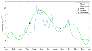
Figure A1 Determining phenology using a combination of threshold method and curve fit at station L4; here the initiation is when the fitted curve is above 50 % of the maximum peak. However, the termination is on the first valley.

This phenology is useful to see how the bloom develops and terminates, whether the concentration increases rapidly and decreases slowly, or vice versa. The phenology is summarized in Fig. A1. The curve fitting method is only applied if the data show potential outliers especially in higher concentrations. If there is only one prominent bloom each year, as at stations ALOHA and BATS, and the data are smooth, the regular threshold method (when the concentration is above 50 % of the maximum bloom, and the associated initiation and termination times) without fitting the data with a curve is applied. To avoid results being affected by how bloom phenology is determined, the same method is used for determining the metrics from both in situ and model output.