the Creative Commons Attribution 4.0 License.
the Creative Commons Attribution 4.0 License.
 | 19 Nov 2018
An improved parameterization of leaf area index (LAI) seasonality in the Canadian Land Surface Scheme (CLASS) and Canadian Terrestrial Ecosystem Model (CTEM) modelling framework
Vivek K. Arora
Joe R. Melton
Paul Bartlett
Leaf area index (LAI) and its seasonal dynamics are key determinants of vegetation productivity in nature and as represented in terrestrial biosphere models seeking to understand land surface atmosphere flux dynamics and its response to climate change. Non-structural carbohydrates (NSCs) and their seasonal variability are known to play a crucial role in seasonal variation in leaf phenology and growth and functioning of plants. The carbon stored in NSC pools provides a buffer during times when supply and demand of carbon are asynchronous. An example of this role is illustrated when NSCs from previous years are used to initiate leaf onset at the arrival of favourable weather conditions. In this study, we incorporate NSC pools and associated parameterizations of new processes in the modelling framework of the Canadian Land Surface Scheme-Canadian Terrestrial Ecosystem Model (CLASS–CTEM) with an aim to improve the seasonality of simulated LAI. The performance of these new parameterizations is evaluated by comparing simulated LAI and atmosphere–land CO2 fluxes to their observation-based estimates, at three sites characterized by broadleaf cold deciduous trees selected from the FLUXNET database. Results show an improvement in leaf onset and offset times with about 2 weeks shift towards earlier times during the year in better agreement with observations. These improvements in simulated LAI help to improve the simulated seasonal cycle of gross primary productivity (GPP) and as a result simulated net ecosystem productivity (NEP) as well.
- Article
(3142 KB) - Full-text XML
-
Supplement
(246 KB) - BibTeX
- EndNote


Biosphere–atmosphere interactions constitute a complex system which plays an important role in the regulation of the climate. These interactions are important determinants governing the physical and chemical properties of the atmosphere as well as the growth of plants and result in the biosphere and atmosphere behaving as a coupled system (Pilegaard et al., 2003). Understanding this coupled behaviour is a key research priority due not only to the important role that terrestrial ecosystems play in modulating the global carbon cycle but also to the significance of land surface characteristics for local and regional climate through biogeophysical effects (Cox et al., 2000; Prentice et al., 2001; Bonan, 2008; Franklin et al., 2016). This growing recognition of the role of land surface vegetation, and its bidirectional interactions with the climate system, has led to ever increasing complexity of the physical and biogeochemical processes that are incorporated in the land surface components of regional and global climate models (Foley et al., 1996; Sitch et al., 2008; Flato et al., 2013). Process-based land surface schemes and ecophysiological models (e.g., Running et al., 1999; Mäkelä et al., 2000; Friend et al., 2007; IPCC, 2013; Sato et al., 2015) simulate atmosphere–land exchanges of carbon, water, and energy and offer tools for understanding vegetation behaviour for the present climate and for projecting vegetation behaviour for future climate scenarios.
The plant canopy is a locus of physical and biogeochemical processes in an ecosystem. The functional and structural attributes of plant canopies are affected by microclimatic conditions, nutrient dynamics, herbivore activities, and many other factors (Asner et al., 2003). Leaves are the point of contact between plants and atmospheric CO2; an increase in leaf area potentially enhances the opportunity for carbon uptake, albeit at the cost of a greater demand for water (Norby et al., 2003). The amount of foliage contained in plant canopies is one of the most basic ecological characteristics that integrates the effects of overall environmental conditions. Canopy leaf area serves as the dominant physical control over primary production (photosynthesis), transpiration, energy exchange, and other physiological attributes pertinent to a range of ecosystem processes and is therefore a core element of ecological field and modelling studies (e.g., Knyazikhin et al., 1998; Xavier and Vettorazzi, 2004; Aboelghar et al., 2010; Gonsamo and Chen, 2014; Bao et al., 2014; Savoy and Mackay, 2015).
Leaf area index (LAI, defined as the amount of leaf area (m2) in the canopy per unit ground area (m2)) is a dimensionless quantity and therefore can be assessed across a range of spatial scales, from individual plant, a forest stand, or grassland to large regions and continents. Leaf phenology describes the response of leaves to seasonal and climatic changes including the timing of bud burst, senescence (leaf maturity or browning), and leaf abscission (leaf fall) and has been documented in a wide range of literature (e.g., Kikuzawa, 1995; Myneni et al., 1997; Arora and Boer, 2005; Menzel et al., 2006; Parmesan, 2006; Richardson et al., 2010; Dragoni et al., 2011; Smith and Hall, 2016). Leaf phenology is a function of environmental conditions (in particular, temperature, soil moisture, and day length). The structural and adaptive qualities specific to vegetation type also determine the timing of leaf phenological events. Accurate prediction of recurring vegetation cycles as a function of climate is an important feature that vegetation models are expected to reproduce. The timing of bud burst and leaf senescence determines the length of the growing season, and this affects gross and net primary productivities (GPP and NPP), the annual cycle of LAI, and consequently the energy, water, and carbon fluxes. The seasonal progression of LAI also influences canopy conductance (Blanken and Black, 2004), albedo (Sakai et al., 1997), and through its modulation of sensible heat (H) and latent heat (LE) fluxes (Moore et al., 1996) also surface air temperatures (Levis and Bonan, 2004).
Despite its importance, the representation of LAI in terrestrial biosphere models is considered poor (Richardson et al., 2012). Lack of high-quality long-term observations, the use of prescribed LAI, simplified formulations of underlying biogeochemical processes, and coarse spatial resolution have been mentioned as some of the limitations to accurate representation of LAI (Kucharik et al., 2006). Since canopy seasonality is an important determinant of carbon (C) fluxes, poor representation of the seasonal dynamics of LAI can lead to inaccurate estimation of vegetation productivity and consequently the net atmosphere–land CO2 flux (Ryu et al., 2008).
Non-structural carbohydrates (NSCs) are the primary products of photosynthesis and a key energy source for plant growth and metabolism. NSCs play a central role in a plant's life processes and its response to the environmental conditions (Kozlowski, 1992; Ögren, 2000; Chatterton et al., 2006; O`Brien et al., 2014; Hartmann and Trumbore, 2016; Sperling et al., 2017). Previous studies have suggested that NSCs are stored in all plant organs (i.e., leaf, branch, root, and stem) at different concentrations that vary seasonally and also inter-annually in response to changes in environmental conditions (e.g., Oberhuber et al., 2011; Bazot et al., 2013; Mei et al., 2015). The amount of NSC and its particular allocation to leaves, stems, and roots are considered ecophysiological traits and are among the range of adaptive strategies that plants use (Li et al., 2001; Poorter and Kitajima, 2007; Wyka et al., 2016). Many factors influence leaf NSC content, including nutrient elements (Zotz and Richter, 2006), temperature (Gough et al., 2010), precipitation (Würth et al., 2005), drought (Rosas et al., 2013), and phenology (Chen et al., 2017). NSC concentrations also vary seasonally and this seasonality has been observed in various plant species (e.g., Zhu et al., 2012; Richardson et al., 2013; Saffell et al., 2014). Despite this extensive research, the size and relative contributions of NSC pools across different tree organs and the movement of NSC amongst the tree organs are not well understood (Friedlingstein et al., 1999; Allen et al., 2005; Sala et al., 2012; Mei et al., 2015).
Plant NSC stores can compensate for a carbon or nitrogen shortage when current demand surpasses supply due to the seasonality of plant growth, stresses, or disturbances. The seasonal dynamics of NSC concentrations have been studied in various plant species (e.g., Zhu et al., 2012; Richardson et al., 2013; Saffell et al., 2014). In deciduous plants, when photosynthesis is constrained by limited leaf area and low temperature in early spring, NSC is mobilized from stem and roots to support respiration and tissue growth, resulting in decreased concentrations of NSC in these storage organs (Hoch et al., 2003; Palacio et al., 2007). During the growing season, storage pools are replenished and NSC concentration increases (Teixeira et al., 2007; Klein et al., 2016). Typically, NSC concentrations in storage organs of the short-lived fast-growing species decrease in springtime after bud flush and then increase during the remainder of the growing season. Correspondingly, the storage organs shift from being a NSC source in the early growing season to becoming a sink in the late growing season, maintaining tree survival after the termination of photosynthate flow from aboveground sources to supply energy for stem and root tissues through the winter (Würth et al., 2005; Gough et al., 2010). During periods of limited photosynthesis, such as winter dormancy or drought stress, trees depend solely on stored NSCs to maintain basic metabolic functions, produce defensive compounds, and retain cell turgor (Sperling et al., 2015). For deciduous species, the NSC storage provides the means to jump-start leaf onset by using a part of NSC stores to push leaves out at the onset of favourable weather conditions (e.g., in spring in the Northern Hemisphere). Representation of NSC pools is therefore an essential step for terrestrial biosphere models to better simulate leaf phenology and seasonal variability in LAI.
Models typically tend not to explicitly represent NSC pools (Le Roux et al., 2001) because of the additional complexity that has to be dealt with unless it is necessary to do so for improved physiological realism of the overall model or representation of a particular physiological process. Those with explicit NSC pools (Dick and Dewar, 1992; Sampson et al., 2001; Ogle and Pacala, 2009; Fisher et al., 2010) may choose to assign no metabolic cost associated with NSC pools and treat it simply as a storage pool from which carbon can be used at a future time (Sala et al., 2012), or they choose to explicitly account for the metabolic carbon costs associated with NSC pools. Existing representations of NSC pools in models have aimed to maintain metabolic function through carbon deficit periods (Sampson et al., 2001), achieve trade-offs between seedling growth and survivorship (Kobe, 1997; Fisher et al., 2010), simulate stress tolerance to ozone (Retzlaff et al., 1996), and represent the response of the respiration ∕ photosynthesis ratio to increase in temperature (Dewar et al., 1999). Models have also used mass balance of NSC pools as a trigger for plant mortality (Dick and Dewar, 1992; Cropper and Gholz, 1993; Sampson et al., 2001; Ogle and Pacala, 2009; Fisher et al., 2010). In terms of model structure, models may have only a single NSC storage pool (Cropper and Gholz, 1993; Kobe, 1997; Schaefer et al., 2008; Ogee et al., 2009) or multiple above- and below-ground pools (Le Dizeìs et al., 1997; Berninger et al., 2000; Allen et al., 2005). Biochemically, models vary in what the NSC pools correspond to. Most models do not distinguish between soluble (e.g., sugars) and insoluble (e.g., starch) NSCs, whereas others may make this distinction (Dick and Dewar, 1992; Le Dizeìs et al., 1997; Dewar et al., 1999; Levy et al., 2000; Geìnard et al., 2008; Schaefer et al., 2008). Dietze et al. (2014) provide a review of existing models which incorporate NSC pools within their framework.
Here, we include a representation of NSC pools and the associated parameterizations in the framework of the Canadian Land Surface Scheme–Canadian Terrestrial Ecosystem Model (CLASS–CTEM). CLASS–CTEM exhibits delayed leaf phenology and we attempt to address this issue. In the original model, the simulated global LAI reaches its maximum in August whereas the observed LAI peaks in July (e.g., see Fig. 11 of Anav et al., 2013). The objective of this study is to improve and assess the performance of CLASS–CTEM simulated leaf phenology for broadleaf cold deciduous trees. Model performance is evaluated against in situ measurements from three sites in the FLUXNET data network (https://fluxnet.ornl.gov/obtain-data, last access: 14 March 2018) which provides tower-based meteorological variables used to drive the model as well as observations of LAI, carbon, and energy fluxes.
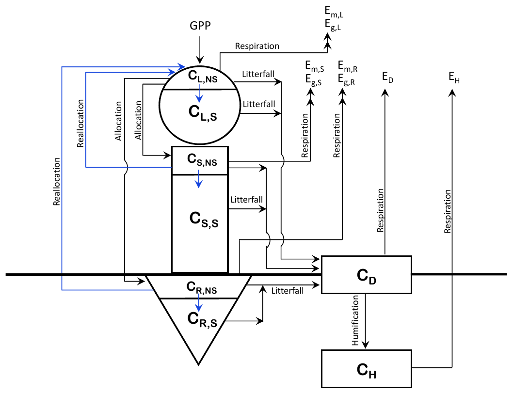
Figure 1Schematic representation of the CTEM model after addition of non-structural carbohydrate pools. The arrows in blue show the new non-structural carbohydrate fluxes as shown in Eqs. (5) and (6).
2.1 CLASS–CTEM model
A coupled version of the Canadian Land Surface Scheme (v. 3.6; Verseghy, 2012) and Canadian Terrestrial Ecosystem Model (v. 2.1.1, Melton and Arora, 2014) (CLASS–CTEM) is used here. Slightly older versions of both models are currently implemented in the second-generation Canadian Earth System Model (CanESM2; Arora et al., 2011). While CLASS simulates fluxes of energy, water, and momentum at the land–atmosphere boundary, atmosphere–land fluxes of CO2 and CH4 are simulated by CTEM. CLASS operates at a typical time step of 30 min and prognostically simulates the liquid and frozen soil moisture and soil temperature for its multiple soil layers (three layers are employed here with maximum thicknesses of 0.1, 0.25, and 3.75 m); the temperature, thickness, and fractional cover of snow; and the temperature and amount of snow and rain on the vegetation canopy. The permeable depth of the soil column may be smaller than the total depth of the soil layers employed; if a layer spans the permeable depth boundary it is subdivided for hydrological calculations. CLASS distinguishes four plant functional types (PFTs) (needleleaf trees, broadleaf trees, crops, and grasses) as shown in Table 1. CLASS calculates net radiation (Rn) based on prognostically calculated land surface albedo and the skin temperature of the land surface (Ts) as
where α is albedo, SW and LW are incoming short- and long-wave radiation, and σ is the Stefan–Boltzmann constant. Rn is partitioned into latent (LE), sensible (H), ground, and canopy heat fluxes. When in equilibrium and over annual and longer time periods, since the ground and canopy do not gain or lose heat systematically, the sum of LE and H fluxes equals net radiation ().
Table 1Plant functional types (PFTs) represented in CTEM and their relation to CLASS PFTs.
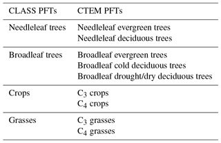
CTEM simulates terrestrial ecosystem processes by prognostically tracking carbon in three living vegetation components (leaves, stems, and roots) and two dead carbon pools (litter and soil) for seven non-crop and two crop PFTs that map directly onto the CLASS PFTs (Table 1). The terrestrial ecosystem processes simulated in this study include photosynthesis, autotrophic respiration, heterotrophic respiration, dynamic leaf phenology, and allocation of carbon from leaves to stem and root components. These processes are described in a sequence of papers detailing parameterization of photosynthesis, autotrophic and heterotrophic respiration (Arora, 2003), dynamic root distribution (Arora and Boer, 2003), phenology, carbon allocation, biomass turnover, and conversion of biomass to structural attributes (Arora and Boer, 2005). A full description of CTEM can be found in the appendix of Melton and Arora (2016) for CO2-related processes and Arora et al. (2018) for CH4-related processes.
The structure of CTEM is shown in Fig. 1; the original three live vegetation pools (leaves, stem, and roots) are indicated by L, S, and R subscripts, respectively, and the two dead carbon pools (litter or detritus and soil carbon) are indicated by D and H subscripts, respectively). Time varying fluxes in and out of these carbon pools (CL, CS, CR, CD, and CH; kg C m−2) makes them prognostic variables in the model. The corresponding rate change equations for amount of carbon in the three live vegetation components (leaves, stem, and roots) in the original model version are represented by
where the index i corresponds to each of the live vegetation pools (), represents allocation fraction for a given vegetation component, Em is vegetation maintenance respiration, Eg is vegetation growth respiration, and Di represents the litter loss. G is canopy GPP and the primary photosynthetic carbon flux which drives all other carbon fluxes in and out of the model's various pools. Although photosynthesis is a function of the total leaf area (LA, m2), model parameterizations use LAI (m2 m−2) since all carbon fluxes and pools are represented per unit of land area.
is the canopy NPP and therefore represents the fraction of NPP allocated to the three vegetation components. Growth respiration, Eg, is estimated as a fraction of the positive gross canopy photosynthetic rate after maintenance respiration has been accounted for (equation A28; Melton and Arora, 2016). is the autotrophic respiration; therefore, . When heterotrophic respiration (Eh) is accounted for, net ecosystem productivity (NEP) is calculated as NEP . Positive NEP values indicate that land is gaining carbon from the atmosphere. Combined autotrophic and heterotrophic respiration (Ea+Eh) are referred to as the ecosystem respiration (Er).
2.1.1 Addition of NSC pools
For the modifications made in this study, first, NSC pools are included in each of the live vegetation components (leaves, stem, and roots). The total biomass (kg C m−2) for each of these components is divided into its non-structural and structural components (indicated by subscripts NS and S) as shown in Fig. 1. and similarly for CS and CR. The fraction of NPP allocated to each live vegetation component is first moved to its non-structural part, and a flux of carbon from the non-structural to the structural part provides carbon to the structural part. Once the carbon is moved from non-structural to a structural part of a component it cannot be moved back. Since NPP includes respiratory losses, this essentially implies that respiratory carbon losses are assumed to occur from the non-structural part. This is consistent with observational and other modelling studies (e.g., Hoch et al., 2003; Sperling et al., 2015; Li et al., 2016), which show that plants' NSC stores become depleted due to respiration during the dormant season and environmental stresses associated with cold temperatures and drought conditions. Litter losses in the model, however, occur from both the structural and non-structural parts of leaves and stem and root components.
The modified rate change equations for carbon in the non-structural and structural parts of leaf (Eq. 3), stem, and root (Eq. 4) components are thus written as
where represents carbon flux from the non-structural to structural part of a component (leaf, stem, or root), and represents the reallocation (or transfer) of carbon from stem and root components to leaves during the leaf-out period (see Sect. 2.1.2). Note that there are no autotrophic respiration terms in Eqs. (3) and (4) since they are already included in the term N, the net primary productivity. Fns2s,i is represented as
where μi is a non-dimensional coefficient set to 70. Equation (5) attempts to keep the fraction of non-structural to total carbon in a component above its minimum specified value . During periods of negative NPP, for example, as is the case during winter for cold deciduous trees when they do not have their leaves on, Fns2s,i is set to zero. This represents the attempts by plants to conserve their NSC pools during a period of no productivity. The amount of carbon in non-structural and structural parts of all vegetation components is shown as time-varying variables and therefore so is the ratio of non-structural to total carbon (ηi). The minimum ratio of non-structural to total carbon in a component () is specified to be 0.05 for the broadleaf cold deciduous PFT considered here, following Li et al. (2016).
The above modifications made to version 2.1.1 of CTEM in regards to the inclusion of NSC pools allow the movement of non-structural carbohydrates among the model's three live vegetation components, in particular, reallocation of non-structural carbohydrates from stem and root components for leaf out at the onset of spring for the broadleaf cold deciduous tree PFT. Distinction between sugar and starch components of NSC pools is not made. This distinction is not necessary to achieve our primary objective of including NSC pools, which is to address the issue of delayed phenology. In addition to incorporating NSC pools, we also adjust allocation fractions for the leaves and stem and root components after summer solstice in response to day length, and we adjust the lower temperature threshold for leaf litter generation due to cold stress. Deciduousness at high latitudes is determined by both day length and temperature (Xie et al., 2015), and these modifications, discussed below, help to improve simulated leaf phenology.
2.1.2 Reallocation of non-structural carbon during leaf-out period
Leaf phenology in CTEM is represented via four phenological states a plant can be in at any given time (Arora and Boer, 2005). These stages include no leaves or dormant state, maximum leaf growth state, normal growth state, and leaf-fall or harvest state. Depending on their deciduousness, CTEM's nine PFTs (Table 1) may or may not go through these four different leaf phenological states. A broadleaf cold deciduous tree transitions through all four states in a year: leafless/dormant state in winter, maximum growth state (following arrival of favourable climatic conditions in spring when all NPP is allocated to leaves), normal growth state (after reaching a threshold LAI, NPP is dynamically allocated to stem and roots in addition to leaves), and finally the leaf-fall state (triggered by unfavourable environmental conditions and with no carbon allocation to leaves). When all the leaves have been shed, the trees go back into the leafless or dormant state again and the cycle repeats itself in the next year. The phenology module of the CLASS–CTEM model is explained in detail in Melton and Arora (2016).
In the original version of the model, when a plant moves into the maximum leaf growth state all NPP is allocated to leaves until a threshold LAI (Lthrs, m2 m−2) has been grown. Lthrs is about 40%–50% of the maximum LAI a plant can support depending on its stem and root biomass and based on an allometric relationship between green and woody biomass (Melton and Arora, 2016). In the absence of NSC pools in the original model version, photosynthesis during the early leaf-out period is based on a small imaginary number of leaves (referred to as storage LAI). Once the actual LAI exceeds the storage LAI then photosynthesis is based on the actual LAI. Storage LAI is proportional to a plant's stem and root biomass and was intended as a proxy for the size of NSC pools. However, the rate of photosynthesis from a reasonably apportioned storage LAI is still too small to realistically “push out” leaves at the onset of spring in a time period of about 2 weeks as seen in observations. This limitation in the original model version is overcome here with the inclusion of NSC pools. In the modified version of the model used here, a specified fraction of carbon amount needed to reach the threshold LAI is reallocated () from a plant's stem and root NSC pools to the non-structural part of leaves every day until LAI reaches Lthrs. Note that while this reallocation occurs the leaves are still able to photosynthesize and able to increase their biomass as in the original model version, depending on meteorological conditions. The objective of carbon reallocation from stem and roots to leaves is to accelerate the rate of leaf expansion and LAI increase during leaf onset.
The amount of carbon reallocated (kg C m−2) from stem and root components to leaves is given by
where SLA is the specific leaf area (m2 kg−1 C−1), β is the reallocation coefficient set to , and fractions ensure that carbon reallocated from stem and root NSC pools is proportional to the size of their NSC pools. Equation (7) also shows that when the fraction of NSC pool relative to total carbon in a component is equal to or drops below its minimum specific value then reallocation is stopped. Reallocation is only performed during the leaf-out state when trees are in the maximum leaf growth state.
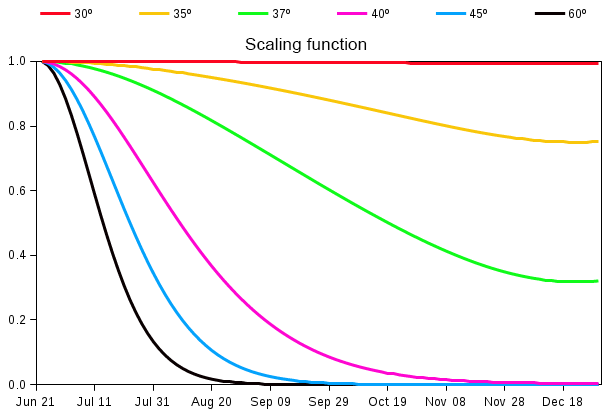
Figure 2Latitude dependence factor (Γ) (Eq. 8) for reducing allocation fraction to leaves after summer solstice.
2.1.3 Adjustments to allocation fraction to leaves after the summer solstice
CTEM uses dynamically calculated allocation fractions (Arora and Boer, 2005; Melton and Arora, 2016) for leaves, stem, and roots, which are based on the light, water, and leaf phenological status of vegetation. The allocation to the three live vegetation components is based on assumptions that carbon is preferentially allocated: (1) to roots when soil moisture is limiting, (2) to leaves when LAI is low, and (3) to the stem to increase vegetation height and lateral spread when increasing LAI leads to a decrease in light penetration. These allocation fractions are superseded by three additional rules: (1) all carbon is allocated to leaves at the time of leaf out for cold deciduous tree PFTs to accelerate leaf development, (2) allocation fractions are adjusted when necessary to ensure a tree has enough stem and root biomass to support leaves (to satisfy a structural allometric relationship), and (3) a minimum realistic root-to-shoot ratio is maintained for all PFTs.
The seasonality of globally averaged LAI is dominated by the response of Northern Hemisphere's vegetation to increasing temperatures in spring and decreasing temperatures in autumn. When compared to observation-based estimates of globally averaged LAI, the CLASS–CTEM-simulated LAI starts to increase later in spring, shows a peak in August (compared to July in observation-based estimates), and exhibits a much slower rate of decline after reaching its annual maximum, which typically occurs just after the summer solstice in each hemisphere (Fig. 11 of Anav et al., 2013). This last issue is addressed by reducing the allocation fraction for leaves () of cold deciduous tree PFTs after summer solstice by multiplication with a day-length-dependent factor (Γ) given by
where d is the day length at latitude ϕ (radian), dmax is its maximum value (h), and δc (radians) is solar declination. Γ varies between 0 and 1 and its behaviour in Fig. 2 shows how allocation to leaves is reduced at a faster (slower) rate closer to poles (Equator) after summer solstice in the Northern Hemisphere (21 June). Below 30∘ N in the Northern Hemisphere Eq. (8) yields Γ=1, so allocation fraction for leaves is not modified. Deciduousness due to day length and temperature typically does not occur in tropics where it is primarily controlled by soil moisture. Neither do broadleaf deciduous cold trees typically exist in the tropics. Similar behaviour is obtained for the Southern Hemisphere after 21 December. Since the allocation fractions for leaves and stem and root components should add to 1, a decrease in allocation fraction for leaves implies an increase in allocation fraction for stem and root components in the modified version of the model. The use of summer solstice to initiate changes in plant behaviour is reasonable since summer solstice is a trigger for many plant physiological processes. Adjustments to allocation fraction for leaves after summer solstice have also been made by Gim et al. (2017) (their Eq. 6). Luo et al. (2018) showed that summer solstice marks a seasonal shift in plant growth, leaf physiology, and foliage turnover in temperate and boreal forests.
In the original version of the CLASS–CTEM model, continuous allocation of carbon to leaves up to the time until they are completely shed led to increase in LAI throughout the growing season rather than a near-constant value or slowly decreasing LAI after the summer solstice.
2.1.4 Adjustments to the lower air temperature threshold
The CLASS–CTEM model is able to respond to environmental conditions and to transition between different leaf phenological states (Arora and Boer, 2005). Leaf litter (DL) generation is caused by normal turnover of leaves as well as drought and cold stresses, which all contribute to LAI seasonality.
where CL is the leaf carbon pool and are the leaf loss rates (day−1) associated with normal (N) turnover of leaves and the cold (C) and drought (D) stresses. The leaf loss rate associated with cold stress (ΩC) is based on Eqs. (A49)–(A50) of Melton and Arora (2016) (shown below as Eq. 11):
where ΩC,max is the maximum leaf loss rate due to cold stress and Lcold is a scalar that varies between 0 and 1 as follows
is a PFT-dependent parameter below which a PFT experiences damage to its leaves and this promotes leaf loss due to cold stress in the model.

Figure 3Location of the three FLUXNET sites chosen in this study to evaluate the changes made to the CLASS–CTEM parameterizations aimed to improve leaf phenology. Figure adapted from Google Maps.
The original version of the model used a parameter value of 8 ∘C throughout the year. In the modified version of the model used here for the broadleaf cold deciduous tree PFT a value of 12 ∘C is used after summer solstice. For the broadleaf cold deciduous tree PFT, leaf out starts in spring, the maximum LAI occurs between July and September (during the Northern Hemisphere's summer), and the leaves are shed between October and November during autumn. Increasing leads to more leaf litter generation due to the cold stress in the autumn and moves the descending side of the LAI curve inwards during autumn.
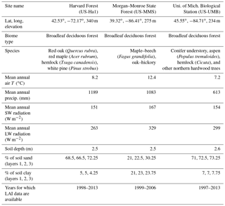
Table 2The location of FLUXNET sites, primary species that exist at these sites, their soil physical characteristics, mean annual values of primary meteorological variables, and years of data availability.
2.2 Model evaluation and experimental set-up
2.2.1 Description of FLUXNET sites
We evaluate the performance of the original and modified versions of the CLASS–CTEM framework in simulating leaf phenology at three well-studied sites in the eastern United States, which are selected from the FLUXNET network: (1) Harvard Forest (US-Ha1) located at 42.53∘ N and 72.17∘ W, (2) Morgan–Monroe State Forest (US-MMS) at 39.32∘ N and 86.41∘ W, and (3) the University of Michigan Biological Station (US-UMB) at 45.55∘ N and 84.71∘ W. The location of the three FLUXNET sites is shown in Fig. 3. The selected sites meet our requirement of availability of observation-based LAI data (against which our model results can be evaluated) and are primarily characterized by deciduous broadleaf forests although with different species composition. The LAI measurements are based on an LAI-2000 plant canopy analyzer instrument and details are provided in Urbanski et al. (2007), Schmid et al. (2000), and Gough et al. (2008) for the Harvard Forest, Morgan–Monroe, and University of Michigan sites, respectively. The mean annual climate at these sites and their species composition are summarized in Table 2. While these sites differ somewhat in the climate they experience, they share enough commonalities in climate to exhibit similar seasonal dynamics of LAI. Annual precipitation at these temperate locations (US-Ha1, US-MMS, and US-UMB) is 1189, 1083, and 613 mm, with an annual mean temperature of 8.2, 12.4, and 7.2 ∘C for each site, respectively. These annual averages are based on the half-hourly meteorological data that are used to drive the CLASS–CTEM model for the time period summarized in Table 2.
The US-Ha1 site is owned by Harvard University. Most of its surrounding area was cleared for agriculture during European settlement in 1600–1700. The trees at the site have been regrowing since before 1900 and are currently characterized by predominantly red oak and red maple, with patches of mature hemlock stand and individual white pine. Climate measurements have been made at the Harvard Forest since 1964. The US-MMS site is owned by the Indiana Department of Natural Resources. Many of the trees in the tower footprint are 60–80 years old. Today, the forest is a secondary successional broadleaf forest within the maple–beech to oak–hickory transition zone of the eastern deciduous forest. Finally, the US-UMB site is located within a protected forest owned by the University of Michigan and consists of mid-aged northern hardwoods, conifer understory, aspen, and old-growth hemlock.
The permeable soil depths are specified at 2.5, 2.5, and 2.62 m at the US-Ha1, US-MMS, and US-UMB sites, respectively. Soil texture information was adapted from the global data set of Zobler (1986) and used to specify the percentage of sand and clay in the model's three soil layers as follows. At US-Ha1, the percentages of sand in the first, second, and third soil layers are specified at 68.5 %, 66.5 %, and 72.25 %, and the percentage of clay at 5 %, 5 %, and 4.25 %, respectively. At US-MMS, the percentages of sand in the first, second, and third soil layers are specified at 21 %, 22.5 %, and 30.25 % and the percentage of clay at 21 %, 23 %, and 23.75 %, respectively. At US-UMB, the percentages of sand in the first, second, and third soil layers are specified at 71 %, 72.5 %, and 73.25 % and the percentage of clay at 7 %, 7 %, and 7.75 %, respectively.
2.2.2 CLASS–CTEM simulations
For the three sites investigated here, we have used version 3.6 of CLASS coupled to version 2.1.1 of the CTEM model and made changes mentioned above in Sect. 2.1. Model performance is evaluated for both the modified and original (without NSC pools) versions against available observation-based estimates of LAI and energy and CO2 fluxes. Simulations were performed for the broadleaf cold deciduous tree PFT with 100 % fractional cover.
Seven meteorological variables are required to drive the CLASS–CTEM model – air temperature, air pressure, wind speed, incoming short-wave radiation, incoming long-wave radiation, precipitation, and specific humidity. FLUXNET's gap-filled meteorological forcing was obtained for each of the three sites. The data were either available at a half-hourly time step or linearly interpolated from hourly to half-hourly resolution. The meteorological data used to drive the model correspond to the period of 1998–2013 for the site in Harvard forest, 1999–2006 for the site in Morgan–Monroe State Forest and 1997–2013 for the site at the University of Michigan Biological Station.
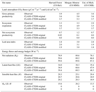
Table 3Simulated and observation-based turbulent energy and carbon fluxes and LAI at the three FLUXNET sites.
All simulations were forced with meteorological data from their respective FLUXNET sites repeatedly until model carbon pools reached equilibrium and the annually averaged NEP was close to zero. A specified atmospheric CO2 concentration of 350 ppm is used at all sites for this spin-up. The real-world forests have, of course, experienced a gradual increase in atmospheric CO2 concentration, changes in climate, and disturbances over their lifetime. Although not perfect, in the absence of full histories of disturbance and meteorological data at these sites this approach still allows comparison of the seasonality of simulated LAI and primary carbon and energy fluxes with observation-based estimates once the model pools reach equilibrium. One caveat is that the modelled vegetation and soil carbon pools cannot be expected to be exactly the same as in the real world but we still expect them to be reasonable. We have chosen to use an atmospheric CO2 concentration of 350 ppm to spin up the model pools (while the average CO2 concentration during the first decade of the 21st century was around 380 ppm) because the terrestrial biosphere is not in equilibrium with the atmospheric CO2 concentration. The disturbance (fire) module was not activated in these simulations. Observation-based LAI measurements were obtained from the AmeriFlux web site (https://ameriflux.lbl.gov, last access: 14 March 2018). Energy and CO2 fluxes were obtained from the FLUXNET web site (https://fluxnet.fluxdata.org, last access: 14 March 2018).
Model performance is evaluated by comparing simulated LAI and CO2 fluxes of GPP and NEP, which is our primary focus. We also compare radiative energy fluxes of Rn and LE and H with their observation-based estimates from the modified and the original model versions.
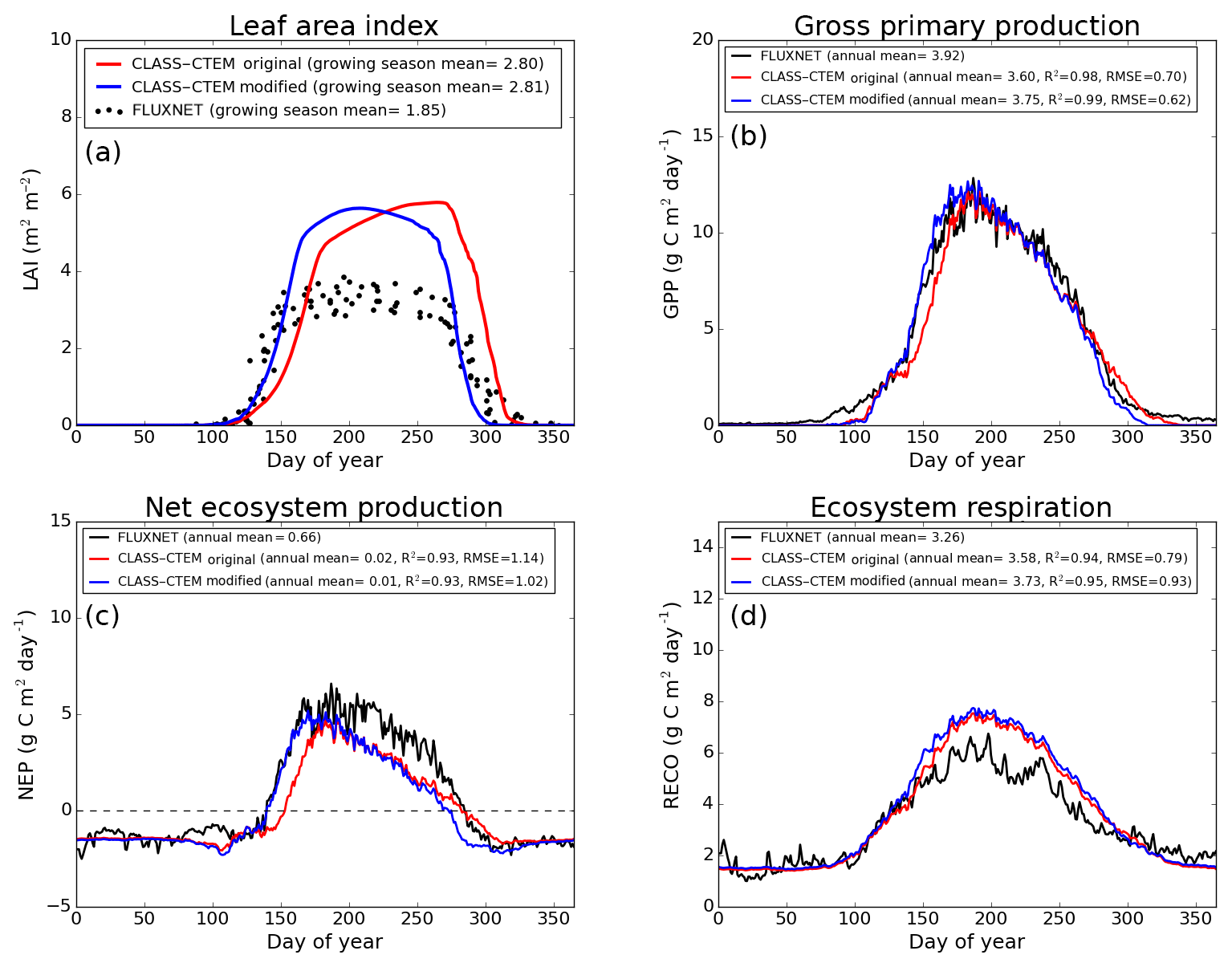
Figure 4Observed and CLASS–CTEM-simulated averaged daily values of (a) LAI (m2 m−2), (b) GPP (g C m−2 day−1), (c) NEP (g C m−2 day−1), and (d) ecosystem respiration (g C m−2 day−1) for the US-Ha1 (Harvard Forest) FLUXNET site across all years when data are present. Legends also show the mean annual value of the quantity plotted, except for LAI, which is averaged over the growing season. Root-mean-square error (RMSE) and coefficient of determination (R2) are also shown for simulated values when compared to observation-based estimates.
3.1 LAI and land–atmosphere CO2 fluxes
Figures 4–6 compare simulated values of LAI, GPP, NEP, and Er from the two model versions with their observation-based estimates at the US-Ha1, US-MMS, and US-UMB FLUXNET sites. Observation-based measurements are shown in black and simulated mean daily values are shown in red (for the original model version indicated as CLASS–CTEM original) and blue (for the modified version, with NSC pools and other changes indicated as CLASS–CTEM modified). Just like simulated values, the observation-based estimates also represent average daily values across all years for which the data were available. The mean annual values of LAI, GPP, Er, and NEP are also summarized in Table 3. At all sites, when compared to the original version, the modified version of the model shows a phenological shift of about 2 weeks earlier in the year, which is in better agreement with observed LAI transitions (Figs. 4a, 5a, and 6a). The timing of maximum LAI also improves and shows a shift of about 2 months earlier in the year, from late September and early October to late July and early August. The observation-based estimates of LAI suggest the presence of understory vegetation at two of the three FLUXNET sites (the Monroe and the Michigan sites). The CLASS–CTEM modelling framework does not represent any understory vegetation. Despite this, the model still overestimates maximum LAI at all locations and its implications are discussed further down. At all three sites, the inclusion of non-structural carbon pools (Sect. 2.1.1) and other model modifications (Sect. 2.1.2 to 2.1.4) produces a notable improvement in simulated LAI seasonality, especially during canopy development (i.e., spring and early summer) and its autumn decline.
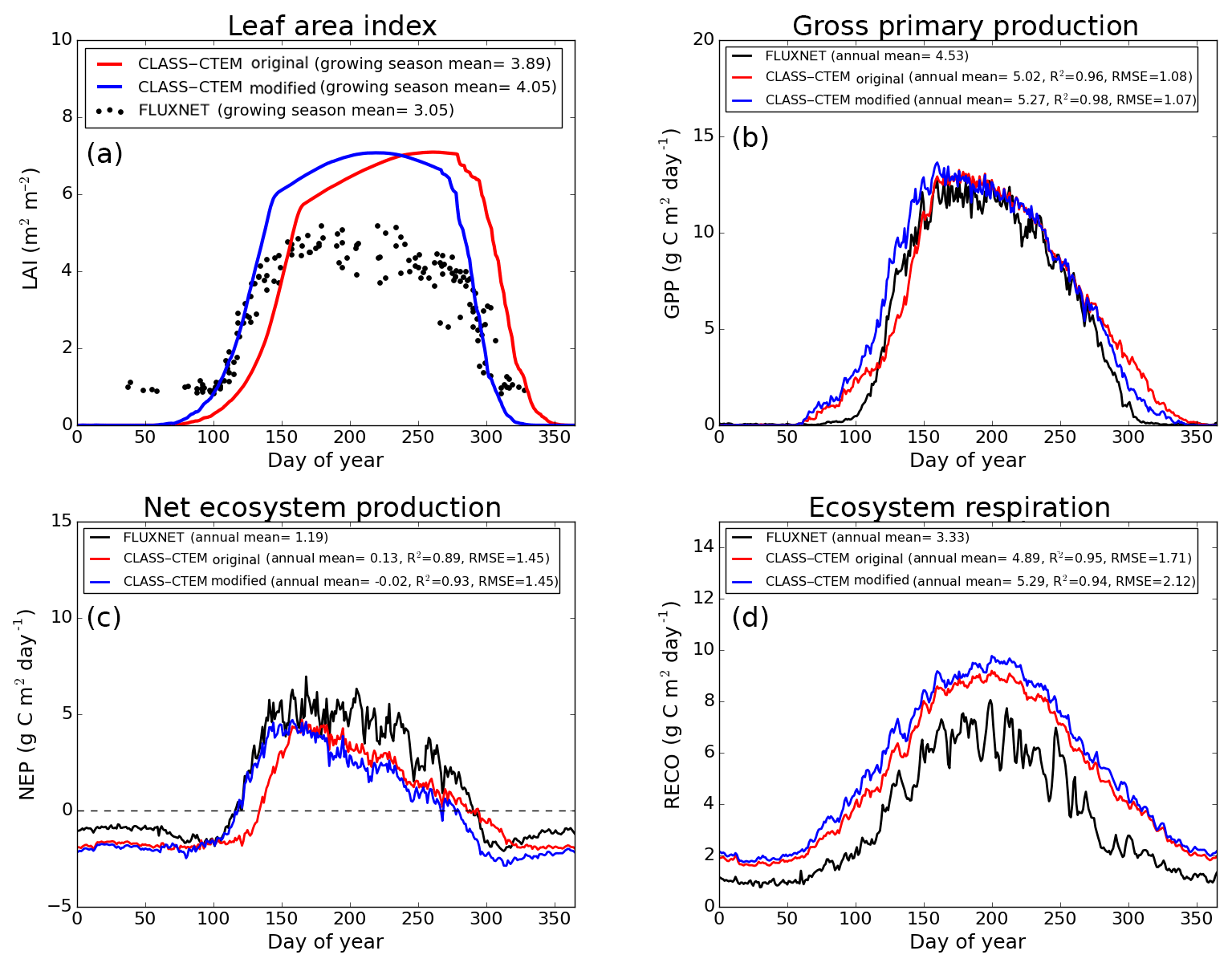
Figure 5Observed and CLASS–CTEM-simulated averaged daily values of (a) LAI (m2 m−2), (b) GPP (g C m−2 day−1), (c) NEP (g C m−2 day−1), and (d) ecosystem respiration (g C m−2 day−1) for the US-MMS (Morgan–Monroe State Forest) FLUXNET site across all years when data are present. Legends also show the mean annual value of the quantity plotted, except for LAI, which is averaged over the growing season. Root-mean-square error (RMSE) and coefficient of determination (R2) are also shown for simulated values when compared to observation-based estimates.
The Morgan–Monroe site (Fig. 5) experiences somewhat warmer temperatures than the Harvard and Michigan sites (Figs. 4 and 6) (mean annual temperature at the Morgan–Monroe is about 4 ∘C higher than at the other two sites; see Table 2) and as a result the growing season is somewhat longer at the Morgan–Monroe site. The model is able to successfully capture this difference amongst the sites. Overall, the simulated GPP and NEP (Figs. 4b, c, 5b, c, 6b, c) compare reasonably well with observations. Improvements in simulated LAI seasonality lead to concomitant improvements in simulated GPP, especially at the ascending side of the plots when the growing season starts. In the original version of the model the increase in GPP at the start of the growing season is delayed due to delayed leaf out. Note that the simulated GPP values compare well with their observation-based estimates despite the higher simulated LAI. Improvements in simulated GPP also lead to improvements in simulated NEP in Figs. 4c, 5c, 6c, and similar to GPP, especially on the ascending side of the plots at the start of the growing season.
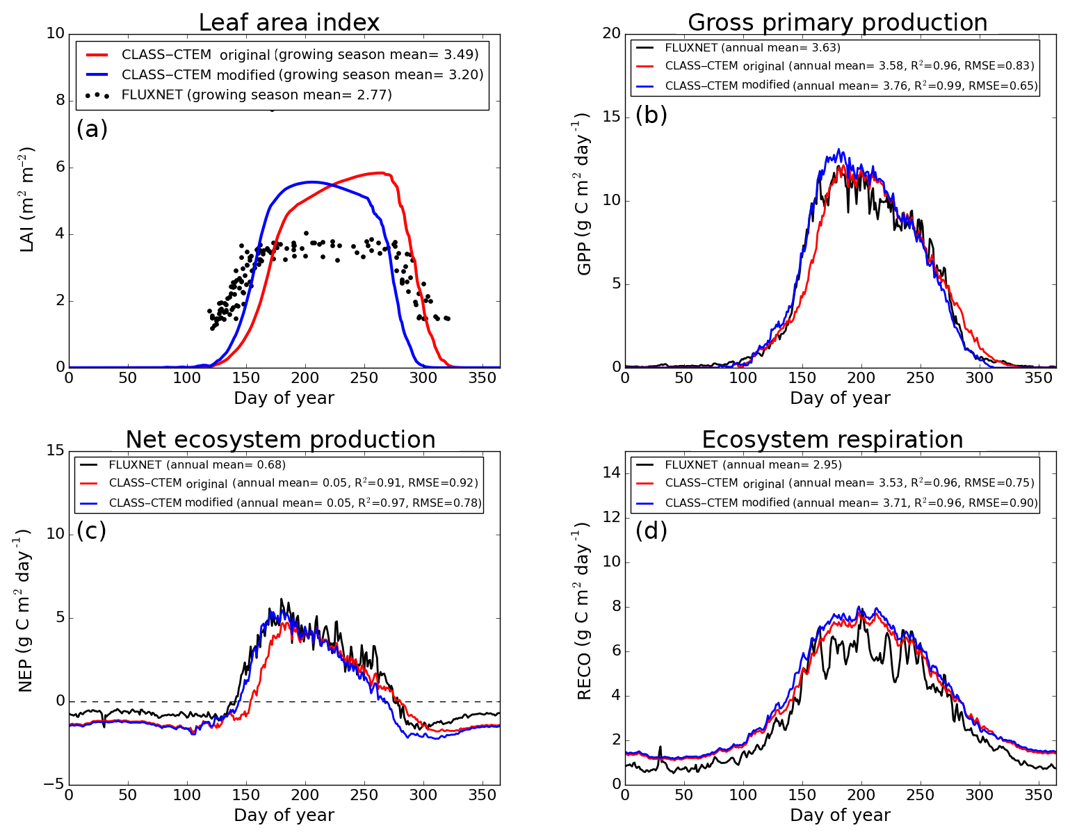
Figure 6Observed and CLASS–CTEM-simulated averaged daily values of (a) LAI (m2 m−2), (b) GPP (g C m−2 day−1), (c) NEP (g C m−2 day−1), and (d) ecosystem respiration (g C m−2 day−1) for the US-UMB (University of Michigan Biological Reserve) FLUXNET site across all years when data are present. Legends also show the mean annual value of the quantity plotted, except for LAI, which is averaged over the growing season. Root-mean-square error (RMSE) and coefficient of determination (R2) are also shown for simulated values when compared to observation-based estimates.
The comparison with observation-based estimates of LAI and GPP is not completely straightforward since the observation-based estimates of these two quantities are put together by different communities and the fact that GPP is a derived quantity (as opposed to NEP, which is directly observed). As a result, the observation-based estimates of LAI and GPP are not completely consistent with each other. This is seen in Fig. 5 for the US-MMS site where the modified version of the model results in a better match with observation-based estimates of LAI (Fig. 5a), but it shows a bias towards an early increase in GPP (Fig. 5b). In contrast, in Fig. 6, the simulated GPP in the modified version of the model compares better with its observation-based estimate than the LAI. In this respect, NEP provides a better measure to assess model improvement than GPP. In Figs. 4 to 6 improvements in simulated LAI in the modified version of the model are more consistent with improvements in simulated NEP.
The individual contributions of the three modifications, (1) inclusion of NSC pools, (2) reduced allocation of carbon to leaves after summer solstice, and (3) change in parameter value of temperature threshold for leaf litter loss due to cold stress, made to the model for resulting improvements in LAI, GPP, and NEP are shown in the Supplement.
The annual mean of observation-based NEP values (as shown in the figure legends of Figs. 4 to 6) is positive because Northern Hemisphere temperate land is currently a sink of carbon (Myneni et al., 2001). In contrast, the annual mean of simulated NEP values is close to zero by construction because the model was spun up to an equilibrium state. The positive annual mean of observation-based NEP values, compared to simulated NEP values, can manifest in multiple ways – as primarily higher summer values when NEP values are positive (as for the Harvard Forest site), as higher values through the year (as is mostly the case at the Morgan–Monroe site), and as less negative NEP values during the non-growing season when NEP values are negative (as seen at the University of Michigan site). Regardless of this caveat, the inclusion of NSC pools to advance leaf onset and offset times does lead to an improvement in seasonality of simulated NEP values.
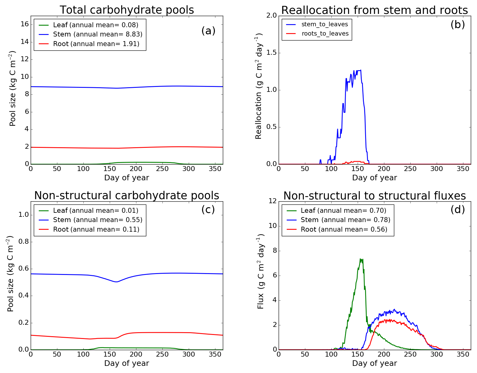
Figure 7CLASS–CTEM (modified version) simulated values of total (a) and non-structural (c) carbohydrate pools (kg C m−2). Panel (b) shows the reallocation of carbon from non-structural stem and root pools to leaves during leaf onset in spring and panel (d) shows the carbon flux from non-structural to structural pools for leaf, stem, and root components (g C m−2 day−1) for the US-Ha1 (Harvard Forest) FLUXNET site. The plots show mean daily values across all years for which the meteorological data were available after the model pools reached equilibrium.
While photosynthesis primarily depends on the current meteorological conditions and LAI amongst other environmental factors (including atmospheric CO2 concentration), ecosystem respiration (Figs. 4d, 5d, 6d) depends strongly on the vegetation and soil carbon pool sizes. As a result, if simulated vegetation and soil carbon pools are larger or smaller than observation-based estimates, then so would be the respiratory fluxes. Note also that the simulated annual respiratory fluxes are higher than observed at all three sites (Figs. 4d, 5d, 6d, and Table 3). Had the simulated fluxes been lower than what they are now and closer to their observation-based estimates, then the simulated NEP would have been more similar to observations. Nevertheless, the model simulates the seasonality of ecosystem respiratory fluxes reasonably well. In absence of the long-term disturbance history or meteorological data to drive the model with, the current methodology (in which the model is driven repeatedly with the available observed meteorological data) is reasonable and allows us to assess the seasonality of simulated LAI and land–atmosphere CO2 fluxes – which is the primary objective of our study.
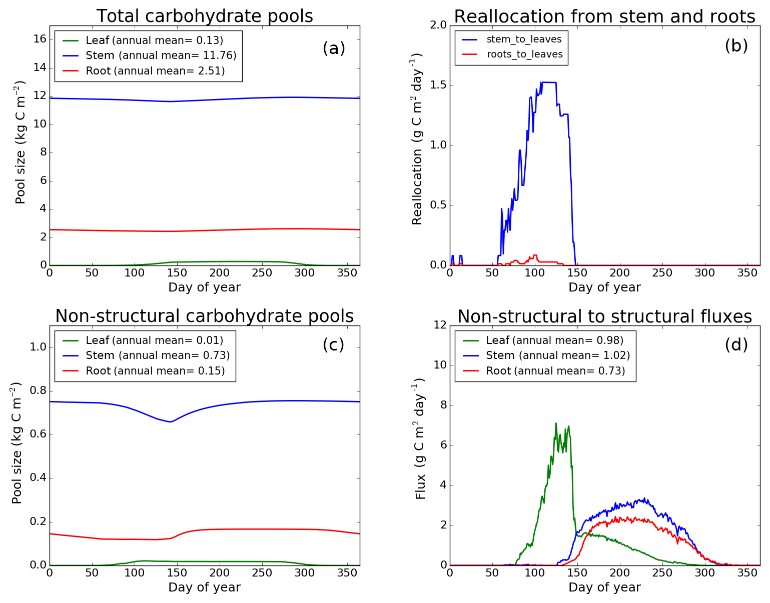
Figure 8CLASS–CTEM (modified version) simulated values of total (a) and non-structural (c) carbohydrate pools (kg C m−2). Panel (b) shows the reallocation of carbon from non-structural stem and root pools to leaves during leaf onset in spring and panel (d) shows the carbon flux from non-structural to structural pools for leaf, stem, and root components (g C m−2 day−1) for the US-MMS (Morgan–Monroe State Forest) FLUXNET site. The plots show mean daily values across all years for which the meteorological data were available after the model pools reached equilibrium.
3.2 NSC pools
Figures 7–9 evaluate the seasonal cycle of the NSC pools in leaf, stem, and root vegetation components at the US-Ha1, US-MMS, and US-UMB FLUXNET sites, respectively. There are no observation-based estimates of NSC pools available at the three FLUXNET sites. For the broadleaf cold deciduous tree PFT considered here, the stem carbon pool is the largest (and so are its structural and non-structural parts) and the leaf carbon pool is the smallest (Figs. 7a, c, 8a, c, 9a, c). The amount of non-structural carbon reallocated from the stem and root NSC pools to leaves during leaf onset in early spring (see Sect. 2.1.2) is shown in Figs. 7b, 8b, 9b. Figures 7d, 8d, 9d show the seasonality of the carbon flux from the non-structural to the structural part of the leaf, stem, and root components for the three sites. The seasonality of total stem and root carbon pools is driven mostly by the seasonality of their non-structural parts.
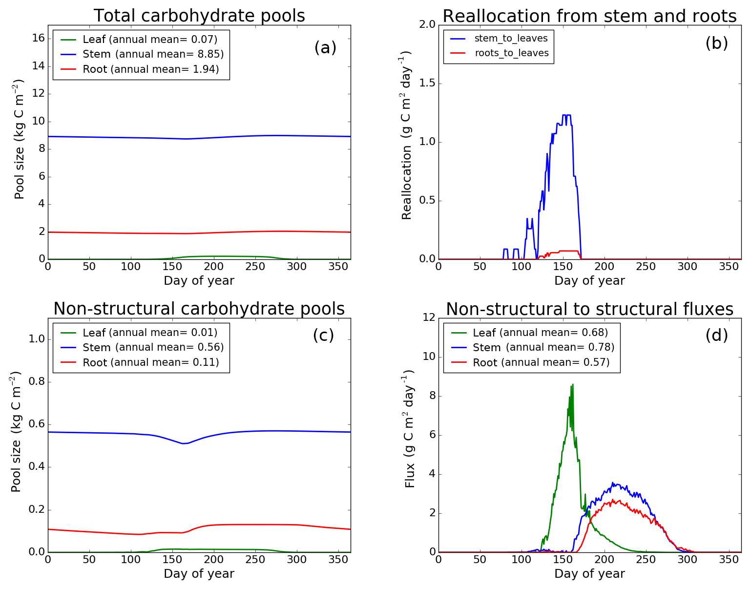
Figure 9CLASS–CTEM (modified version) simulated values of total (a) and non-structural (c) carbohydrate pools (kg C m−2). Panel (b) shows the reallocation of carbon from non-structural stem and root pools to leaves during leaf onset in spring and panel (d) shows the carbon flux from non-structural to structural pools for leaf, stem, and root components (g C m−2 day−1) for the US-UMB (University of Michigan Biological Reserve) FLUXNET site. The plots show mean daily values across all years for which the meteorological data were available after the model pools reached equilibrium.
For the stem and root components, the non-structural parts contribute about 6 %–10 % to the total pool size. During the early leaf-out period when reallocation from stem and root NSC pools to leaves is taking place (Sect. 2.1.2), the stem's NSC pool becomes depleted. This transfer/reallocation stops after a threshold LAI is achieved. The transfer of NSC from stem and root pools to leaves occurs mostly through the stem (see Figs. 7b, 8b, 9b) since its NSC pool is about 3–4 times larger than the root component. The NSC pool for both components reduces during the period when leaves are not present (and GPP is zero) due to respiratory and litter losses. The pools for both stem and root components are replenished later during the growing season when a sufficient number of leaves have been grown and allocation of carbon to stem and root components is restored. This is seen in Figs. 7d, 8d, 9d), which show the flux of carbon from non-structural to structural leaf, stem, and root components. Early on during the growing season, carbon flux from the leaf NSC pool to its structural part is much higher since the model preferably allocates carbon to leaves as discussed in Sect. 2.1.2. After a threshold LAI is reached, carbon is also allocated to stem and root NSC pools, which subsequently start to allocate carbon to their structural pools and the tree biomass continues to increase. At the end of the growing season, when photosynthesis stops, allocation to all three components and the fluxes from NSC to structural parts terminate. During the dormant winter season NSC pools provide for the respiratory costs.

Figure 10Observed and CLASS–CTEM-simulated daily net radiation (W m−2), latent heat flux (W m−2), and sensible heat flux (W m−2) for the three FLUXNET sites. Legends also show the mean annual value of the quantity plotted. Root-mean-square error (RMSE) and coefficient of determination (R2) are also shown for simulated values when compared to observation-based estimates.
3.3 Energy fluxes
Figure 10 compares observation-based measurements of LE, H, and Rn fluxes at the three FLUXNET sites, with their simulated values from the two model versions. Annual mean values of these observation-based and simulated radiative and turbulent energy fluxes are also summarized in Table 3. Unlike the simulated fluxes, the annual mean sum of the observed LE and H, averaged over the years for which observations are available, is not equal to the observed Rn. This non-closure of the energy budget is seen at all three sites and is a typical characteristic of eddy-covariance-based flux measurements (Gao et al., 2017). The annual energy budget closure is off by 17 % at the University of Michigan Biological Station, by 20 % at the Harvard Forest, and by 30 % at the Morgan–Monroe sites as seen in Table 3. Keeping this caveat in mind, the model captures the seasonality of radiative and turbulent fluxes shown in Fig. 10 reasonably overall, with the exception of late winter and early spring. During this period, as solar radiation increases Rn is underestimated (Fig. 10a–c) until the canopy approaches a full-leaf state and this leads to an underestimation of H (Fig. 10g–i) and overestimation of LE. This may be caused by an overestimation of canopy transmissivity and underestimation of snow and soil masking by leafless forests with increasing solar elevation (recently observed in unpublished simulations with CLASS–CTEM at the Borden forest, Borden, Ontario, Canada) and may also be exacerbated by the lack of representation of a small evergreen needleleaf fraction at US-Ha1 and a conifer understory at US-UMB. LE is apparently overestimated throughout the year at US-MMS but we suspect this reflects a larger underestimation of LE relative to H in the measured fluxes; Oliphant et al. (2004) found that accounting for long sampling tube damping effects on LE resulted in a 16 % improvement in energy balance closure at this site. The change to an earlier leaf phenology in the modified simulations results in a slightly earlier increase in LE in the spring as well as slightly earlier decreases in autumn at US-Ha1 and US-UMB, but differences are much smaller at US-MMS.
In Fig. 10 the changes in LAI, due to modifications made to the original version of the model, do not significantly affect LE fluxes because of two related reasons. First, at mid- to high-latitude locations where soil moisture constraint is not very large, as is the case at the three sites considered in this study, total evapotranspiration (or LE flux) is controlled by available energy. This is the reason for the expected seasonality in LE flux at these sites, which is characterized by higher values during summer and lower values during winter. Second, since the LE flux at these three sites is controlled primarily by available energy, the resulting implication is that if evaporative demand cannot be met by transpiration then it will be met by evaporation from the soil. As a result, changes in LAI do not significantly affect total evapotranspiration but change the partitioning of evapotranspiration flux coming from transpiration, evaporation of intercepted water on canopy leaves, and evaporation from the soil.
The CLASS–CTEM model, similar to other land surface schemes implemented in other Earth system models, is not tuned for any specific location but is expected to behave realistically at all locations. Model processes correspond to generic PFTs, in this case broadleaf cold deciduous trees, and are not meant to represent specific species differences within a PFT. It is nearly impossible, at present, to determine more than 100 parameters for individual species for the CLASS–CTEM model. As a result, while our three chosen sites are characterized by different species (as shown in Table 2), they must be represented by a single set of parameter values which correspond to the broadleaf cold deciduous PFT.
Previous studies using the CLASS–CTEM model in the context of land–atmosphere CO2 fluxes and simulated carbon pools have evaluated its performance at point (Arora, 2003; Arora and Boer, 2005; Melton et al., 2015), regional (Garnaud et al., 2015; Peng et al., 2014; Arora et al., 2016), and global (Arora and Boer, 2010; Melton and Arora, 2014, 2016) scales. These studies indicate that the model performance is reasonable. CLASS–CTEM also participated in the TRENDY model intercomparison, the result of which contributed to the Global Carbon Project for the years 2016 and 2017 (Le Quéré et al., 2016, 2018). A typical model evaluation exercise at the global and regional scale compares model-simulated geographical distribution of GPP, vegetation biomass, and soil carbon with their respective observation-based estimates. Point-scale studies, however, typically focus on the simulated seasonality of energy and CO2 fluxes as is the case in this study. Model evaluation exercises not only help in identifying model limitations but also yield opportunities to improve model performance by tuning model parameters.
We chose to perform equilibrium simulations by forcing the model repeatedly with available meteorological data at a specified CO2 concentration of 350 ppm. In the absence of meteorological data that show a warming trend over the historical period we would not have been able to properly perform a historical simulation. Our past experience shows that steady-state simulations, as opposed to historical transient simulations, allow an easier interpretation of model modifications in the absence of confounding effects of changing climate and increasing CO2.
Previous evaluations of the CLASS–CTEM model that highlighted its limitation of delayed leaf phenology (e.g., Anav et al., 2013) were the motivation for this study. NSC pools play an important role during leaf onset for broadleaf deciduous cold trees, but also other PFTs, and their effect in the original model was represented using the concept of imaginary leaves whose LAI is assumed to be directly proportional to non-leaf biomass. Here, we have explicitly included NSC pools in the model framework along with some other changes and these modifications do lead to improvement in simulated leaf phenology and concomitant improvements in the simulated seasonal cycle of GPP and NEP. Improvements in simulated energy fluxes are much harder to detect because the observation-based energy fluxes are affected by non-closure of the energy budget but also because LE fluxes are not as strongly dependent on LAI as GPP.
Despite the simulated LAI being higher than observation-based estimates, the simulated GPP, Er, and NEP compare reasonably with their observation-based estimates. Possible reasons for higher simulated LAI include higher-than-observed allocation to leaf compared to stem and root components and lower-than-observed leaf turnover and/or leaf respiration rates. The model currently uses a maximum carboxylation capacity (Vc,max, i.e., maximum photosynthetic rate) value of 57 µmol CO2 m−2 s−1 for broadleaf cold deciduous trees based on Table 3 of Kattge et al. (2009), who derive Vc,max values for major PFTs using more than 700 data estimates. While in the CLASS–CTEM model photosynthesis is also limited by light and transport capacity rates in addition to carboxylation capacity (see Appendix A2 in Melton and Arora, 2016), Vc,max remains a strong parameter and simulated GPP in the model is proportional to Vc,max. While the model-simulated LAI can be lowered by tuning allocation to leaves, leaf turnover, and/or respiration rates specifically for these sites, this would imply using a Vc,max value higher than that suggested by Kattge et al. (2009) to achieve realistic GPP. It is possible that the average Vc,max value derived by Kattge et al. (2009) is not representative of broadleaf cold deciduous trees in the eastern United States. The simulated LAI in the model is the result of multiple model processes interacting with each other. We note this limitation of the model at these locations and plan to address it in the near future. While LAI is an important determinant of model performance, even more important are the land–atmosphere CO2 fluxes from an Earth system model perspective since it is the CO2 fluxes which determine the carbon budget of the atmosphere in a fully coupled Earth system model simulation (Arora et al., 2013).
Plants are extremely complex living organisms which respond to the changes in their physical and chemical environmental conditions using a myriad of adaptations. Our limited understanding of these adaptations comes only from empirical observations of their behaviour and measurement of their physical and chemical responses to environmental changes. Models typically represent only a fraction of this understanding because model structures depend on the purpose of the model and the number of details that can be represented reasonably in a model's framework. In hindsight, the omission of NSC pools in the original model version was a structural error and while the conceptual imaginary leaves tried to mimic the fast growth rate of leaves during leaf onset at the arrival of favourable environmental conditions, they were not completely successful in capturing the real-world behaviour. In addition, in a past exercise, we also used higher Vc,max values at the beginning of the growing season to accelerate the rate of growth of leaves (based on Bauerle et al., 2012, and Alton, 2017) but this also did not sufficiently help to address the slower-than-observed rate of growth of LAI at the start of the growing season. Unlike physical models, which describe a physical process, modelling of biological response to changes in environmental conditions is more complex. While there may be underlying physical laws that determine the response of plants to changes in environmental conditions, we can only interpret this from a biological point of view. Dynamic vegetation models and land surface schemes parameterize biological functioning using mathematical formulations to reproduce empirical observations and modellers' conceptual understanding of how the biology works. The inclusion of NSC pools in the CLASS–CTEM framework is based on the same philosophy.
The implementation of NSC pools in the CLASS–CTEM modelling framework presented in this study is meant specifically to address the problem of delayed leaf phenology. NSC pools also play a vital role in the overall health of the plants as mentioned earlier in the introductory section. During periods of limited photosynthesis, trees depend solely on stored NSCs to maintain basic metabolic functions, produce defensive compounds, and retain cell turgor (Sperling et al., 2015). A period of continuous drought, for instance, will gradually reduce the size of NSC pools and this can be used as a trigger to initiate drought-related mortality in the model, or alternatively NSC pools may be used to allow leaf growth during a short-term dry period to represent resilience (Mitchell et al., 2013). The inclusion of NSC pools, also lays the groundwork to implement a nitrogen (N) cycle in the CLASS–CTEM framework since modelling Vc,max as a function of leaf N content requires leaf N content in the non-structural part of the leaves.
In conclusion, modifications to the CLASS–CTEM framework made in this study to address the problem of delayed leaf phenology yield improvements to simulated seasonality of LAI at the three FLUXNET sites considered here. These improvements, especially the inclusion of NSC pools also lay the groundwork for future model development and inclusion of new processes.
The model code is available at https://gitlab.com/jormelton/classctem (Melton, 2018) but requires resgistration on gitlab.com. The observation-based data used in this paper can be obtained from the FLUXNET (https://fluxnet.ornl.gov/obtain-data, ORNL DAAC, 2018) and AmeriFlux (https://ameriflux.lbl.gov, AmeriFlux Network, 2018) data networks. Model-simulated data can be obtained from the second author (vivek.arora@canada.ca).
The supplement related to this article is available online at: https://doi.org/10.5194/bg-15-6885-2018-supplement.
AA performed the experiments, reviewed the relevant literature, and wrote the majority of the paper. VKA wrote and revised several parts of the paper and supervised and helped AA to set up and run the CLASS–CTEM model. PB contributed to the writing of the energy flux part of the paper (Sect. 3.3). JRM helped to set up the modelling framework.
The authors declare that they have no conflict of interest.
Ali Asaadi was supported by a National Scientific and Engineering Research
Council of Canada (NSERC) visiting postdoctoral fellowship. We thank the FLUXNET
and AmeriFlux data networks for providing the data used in our study. We
would also like to thank Philip Savoy for sharing LAI data for the
Morgan–Monroe site investigated in this study. We are also grateful to
Reinel Sospedra-Alfonso and Michael Sigmond for providing comments on an
earlier version of this paper.
Edited
by: Akihiko Ito
Reviewed by: two anonymous referees
Aboelghar, M., Arafat, S., Saleh, A., Naeem, S., Shirbeny, M., and Belal, A.: Retrieving leaf area index from SPOT4 satellite data Egypt, J. Remote Sens. Space Sci., 13, 121–127, 2010.
AmeriFlux Network: AmeriFlux, availabl at: https://ameriflux.lbl.gov), last access: 14 March 2018.
Allen, M. T., Prusinkiewicz, P., and DeJong, T. M.: Using L-systems for modeling source-sink interactions, architecture and physiology of growing trees: the L-PEACH model, New Phytol., 166, 869–880, 2005.
Alton, P. B.: Retrieval of seasonal rubisco-limited photosynthetic capacity at global FLUXNET sites from hyperspectral satellite remote sensing: Impact on carbon modelling, Agr. Forest Meteorol., 232, 74–88, 2017.
Anav, A., Friedlingstein, P., Kidston, M., Bopp, L., Ciais, P., Cox, P., Jones, C., Jung, M., Myneni, R., and Zhu, Z.: Evaluating the land and ocean components of the global carbon cycle in the CMIP5 earth system models, J. Clim., 26, 6801–6843, 2013.
Arora, V. K.: Simulating energy and carbon fluxes over winter wheat using coupled land surface and terrestrial ecosystem models, Agr. Forest Meteorol., 118, 21–47, 2003.
Arora, V. K. and Boer, G. J.: A representation of variable root distribution in dynamic vegetation models, Earth Interact., 7, 1–19, 2003.
Arora, V. K. and Boer, G. J.: A parameterization of leaf phenology for the terrestrial ecosystem component of climate models, Glob. Change Biol., 11, 39–59, 2005.
Arora, V. K. and Boer, G. J. : Uncertainties in the 20th century carbon budget associated with land use change, Glob. Change Biol., 16, 3327–3348, 2010.
Arora, V. K., Scinocca, J. F., Boer, G. J., Christian, J. R., Denman, K. L., Flato, G. M., Kharin, V. V., Lee, W. G., and Merryfield, W. J.: Carbon emission limits required to satisfy future representative concentration pathways of greenhouse gases, Geophys. Res. Lett., 38, L05805, https://doi.org/10.1029/2010GL046270, 2011.
Arora, V. K., Boer, G. J., Friedlingstein, P., Eby, M., Jones, C. D., Christian, J. R., Bonan, G., Bopp, L., Brovkin, V., Cadule, P., Hajima, T., Ilyina, T., Lindsay, K., Tjiputra, J. F., and Wu, T.: Carbon-concentration and carbon-climate feedbacks in CMIP5 earth system models, J. Clim., 26, 5289–5314, 2013.
Arora, V. K., Peng, Y., Kurz, W. A., Fyfe, J. C., Hawkins, B., and Werner, A. T.: Potential near-future carbon uptake overcomes losses from a large insect outbreak in British Columbia, Canada, Geophys. Res. Lett., 43, 2590–2598, 2016.
Arora, V. K., Melton, J. R., and Plummer, D.: An assessment of natural methane fluxes simulated by the CLASS-CTEM model, Biogeosciences, 15, 4683–4709, https://doi.org/10.5194/bg-15-4683-2018, 2018.
Asner, G. P., Scurlock, J. M. O., and Hicke, J. A.: Global synthesis of leaf area index observations: Implications for ecological and remote sensing studies, Global Ecol. Biogeogr., 12, 191–205, 2003.
Bao, Y., Gao, Y., Lü, S., Wang, Q., Zhang, S., Xu, J., Li, R., Li, S., Ma, D., Meng, X., Chen, H., and Chang, Y.: Evaluation of CMIP5 earth system models in reproducing leaf area index and vegetation cover over the Tibetan Plateau, J. Meteor. Res., 28, 1041–1060, 2014.
Bauerle, W. L., Oren, R., Way, D. A., Qian, S. S., Stoy, P. C., Thornton, P. E., Bowden, J. D., Hoffman, F. M., and Reynolds, R. F.: Photoperiodic regulation of the seasonal pattern of photosynthetic capacity and the implications for carbon cycling, P. Natl. Acad. Sci. USA, 109, 8612–8617, 2012.
Bazot, S., Barthes, L., Blanot, D., and Fresneau, C.: Distribution of non-structural nitrogen and carbohydrate compounds in mature oak trees in a temperate forest at four key phenological stages, Trees, 27, 1023–1034, 2013.
Berninger, F., Nikinmaa, E., Sievanen, R., and Nygren, P.: Modelling of reserve carbohydrate dynamics, regrowth and nodulation in a N2-fixing tree managed by periodic prunings, Plant Cell Environ., 23, 1025–1040, 2000.
Blanken, P. D. and Black, T. A.: The canopy conductance of a boreal aspen forest, Prince Albert National Park, Canada, Hydrol. Process., 18, 1561–1578, 2004.
Bonan, G. B.: Forests and climate change: forcings, feedbacks, and the climate benefits of forests, Science, 320, 1444–1449, 2008.
Chatterton, N. J., Watts, K. A., Jensen, K. B., Harrison, P. A., and Horton, W. H.: Nonstructural carbohydrates in oat forage, J. Nutr., 136, 2111S–2113S, 2006.
Chen, Z., Wang, L., Dai, Y., Wan, X., and Liu, S.: Phenology-dependent variation in the non-structural carbohydrates of broadleaf evergreen species plays an important role in determining tolerance to defoliation (or herbivory), Sci. Rep., 7, 10125, https://doi.org/10.1038/s41598-017-09757-2, 2017.
Cox, P. M., Betts, R. A., Jones, C. D., Spall, S. A., and Totterdell, I. J.: Acceleration of global warming due to carbon-cycle feedbacks in a coupled climate model, Nature, 408, 184–187, 2000.
Cropper, W. P. and Gholz, H. L.: Simulation of the carbon dynamics of a Florida slash pine plantation, Ecol. Model., 66, 231–249, 1993.
Dewar, R. C., Medlyn, B. E., and McMurtrie, R. E.: Acclimation of the respiration photosynthesis ratio to temperature: insights from a model, Glob. Change Biol., 5, 615–622, 1999.
Dick, J. M. and Dewar, R. C.: A mechanistic model of carbohydrate dynamics during adventitious root development in leafy cuttings, Ann. Bot., 70, 371–377, 1992.
Dietze, M. C., Sala, A., Carbone, M. S., Czimczik, C. I., Mantooth, J. A., Richardson, A. D., and Vargas, R.: Nonstructural carbon in woody plants, Annu. Rev. Plant Biol., 65, 667–687, 2014.
Dragoni, D., Schmid, H. P., Wayson, C. A., Potter, H., Grimmond, C. S. B., and Randolph, J. C.: Evidence of increased net ecosystem productivity associated with a longer vegetated season in a deciduous forest in south-central Indiana, USA, Glob. Change Biol., 17, 886–897, 2011.
Fisher, R., McDowell, N., Purves, D., Moorcroft, P., Sitch, S., Cox, P., Huntingford, C., Meir, P., and Woodward, F. I.: Assessing uncertainties in a second-generation dynamic vegetation model caused by ecological scale limitations, New Phytol., 187, 666–681, 2010.
Flato, G., Marotzke, J., Abiodun, B., Braconnot, P., Chou, S. C., Collins, W., Cox, P., Driouech, F., Emori, S., Eyring, V., Forest, C., Gleckler, P., Guilyardi, E., Jakob, C., Kattsov, V., Reason, C., and Rummukainen, M., Evaluation of Climate Models, in: Climate Change 2013: The Physical Science Basis. Contribution of Working Group I to the Fifth Assessment Report of the Intergovernmental Panel on Climate Change, edited by: Stocker, T. F., Qin, D., Plattner, G.-K., Tignor, M., Allen, S. K., Boschung, J., Nauels, A., Xia, Y., Bex, V., and Midgley, P. M., Cambridge Univ. Press, Cambridge, United Kingdom and New York, NY, USA, 741–866, 2013.
Foley, J. A., Prentice, I. C., Ramankutty, N., Levis, S., Pollard, D., Sitch, S., and Haxeltine, A.: An integrated biosphere model of land surface processes, terrestrial carbon balance and vegetation dynamics, Global Biogeochem. Cy., 10, 603–628, 1996.
Franklin, J., Serra-Diaz, J. M., Syphard, A. D., and Regan, H. M.: Global change and terrestrial plant community dynamics, P. Natl. Acad. Sci. USA, 113, 3725–3734, 2016.
Friedlingstein, P., Joel, G., Field, C. B., and Fung, I. Y.: Toward an allocation scheme for global terrestrial carbon models, Glob. Change Biol., 5, 755–770, 1999.
Friend, A., Arneth, A., Kiang, N., Lomas, M., Ogee, J., Roedenbeck, C., Running, S., Santaren, J., Sitch, S., Viovy, N., Woodward, I., and Zaehle, S.: Fluxnet and modelling the global carbon cycle, Glob. Change Biol., 13, 610–633, 2007.
Gao, Z., Liu, H., Katul, G. G., and Foken, T.: Non-closure of the surface energy balance explained by phase difference between vertical velocity and scalars of large atmospheric eddies, Environ. Res. Lett., 12, 034025, https://doi.org/10.1088/1748-9326/aa625b, 2017.
Garnaud, C., Sushama, L., and Verseghy, D. L.: Impact of interactive vegetation phenology on the Canadian RCM simulated climate over North Americ, Clim. Dynam., 45, 1471–1492, 2015.
Geìnard, M., Dauzat, J., Franck, N., Lescourret, F., Moitrier, N., Vaast, P., and Vercambre, G.: Carbon allocation in fruit trees: from theory to modelling, Trees, 22, 269–282, 2008.
Gim, H.-J., Park, S. K., Kang, M., Thakuri, B. M., Kim, J., and Ho, C.-H.: An improved parameterization of the allocation of assimilated carbon to plant parts in vegetation dynamics for Noah-MP, J. Adv. Model. Earth Sy., 9, 1776–1794, 2017.
Gonsamo, A. and Chen, J. M.: Continuous observation of leaf area index at Fluxnet-Canada sites, Agr. Forest Meteorol., 189, 168–174, 2014.
Gough, C. M., Vogel, C. S., Schmid, H. P., Su, H. B., and Curtis, P. S.: Multi-year convergence of biometric and meteorological estimates of forest carbon storage, Agr. Forest Meteorol., 148, 158–170, 2008.
Gough, C. M., Flower, C. E., Vogel, C. S., and Curtis, P. S.: Phenological and temperature controls on the temporal non-structural carbohydrate dynamics of Populus grandidentata and Quercus rubra, Forests, 1, 65–81, 2010.
Hartmann, H. and Trumbore, S.: Understanding the roles of nonstructural carbohydrates in forest trees – from what we can measure to what we want to know, New Phytol., 211, 386–403, 2016.
Hoch, G., Popp, M., and Körner, C.: Altitudinal increase of mobile carbon pools in Pinus cembra suggest sink limitation at the Swiss treeline, Oikos, 98, 361–374, 2002.
Hoch, G., Richter, A., and Körner, C.: Non-structural carbon compounds in temperate forest trees, Plant Cell Environ., 26, 1067–1081, 2003.
IPCC: Summary for Policymakers, in: Climate Change 2013: The Physical Science Basis, in: Contribution of Working Group I to the Fifth Assessment Report of the Intergovernmental Panel on Climate Change, edited by: Stocker, T. F., Qin, D., Plattner, G.-K., Tignor, M., Allen, S. K., Boschung, J., Nauels, A., Xia, Y., Bex, V., and Midgley, P. M., Cambridge University Press, Cambridge, United Kingdom and New York, NY, USA, 2013.
Kattge, J., Knorr, W., Raddatz, T., and Wirth, C.: Quantifying photosynthetic capacity and its relationship to leaf nitrogen content for global-scale terrestrial biosphere models, Glob. Change Biol., 15, 976–991, 2009.
Kikuzawa, K.: Leaf phenology as an optimal strategy for carbon gain in plants, Can. J. Bot., 73, 158–163, 1995.
Klein, T., Vitasse, Y., and Hoch, G.: Coordination between growth, phenology and carbon storage in three coexisting deciduous tree species in a temperate forest, Tree Physiol., 36, 847–855, 2016.
Knyazikhin, Y., Martonchik, J. V., Diner, D. J., Myneni, R. B., Verstraete, M., Pinty, B., and Gobron, N.: Estimation of vegetation canopy leaf area index and fraction of absorbed photosynthetically active radiation from atmosphere-corrected MISR data, J. Geophys. Res., 103, 32239–32256, 1998.
Kobe, R. K.: Carbohydrate allocation to storage as a basis of interspecific variation in sapling survivorship and growth, Oikos, 80, 226–33, 1997.
Kozlowski, T. T.: Carbohydrate sources and sinks in woody plants, Bot. Rev., 58, 107–222, 1992.
Kucharik C. J., Barford, C. C., Maayar, M. E., Wofsy, S. C., Monson, R. K., and Baldocchi, D. D.: A multiyear evaluation of a dynamic global vegetation model at three ameriflux forest sites: vegetation structure, phenology, soil temperature, and CO2 and H2O vapor exchange, Ecol. Modell., 196, 1–31, 2006.
Le Dizeìs, S., Cruiziat, P., Lacointe, A., Sinoquet, H., Le Roux, X., Balandier, P., and Jacquet, P.: A model for simulating structure-function relationships in walnut tree growth processes, Silva Fenn., 31, 313–328, 1997.
Le Quéré, C., Andrew, R. M., Canadell, J. G., Sitch, S., Korsbakken, J. I., Peters, G. P., Manning, A. C., Boden, T. A., Tans, P. P., Houghton, R. A., Keeling, R. F., Alin, S., Andrews, O. D., Anthoni, P., Barbero, L., Bopp, L., Chevallier, F., Chini, L. P., Ciais, P., Currie, K., Delire, C., Doney, S. C., Friedlingstein, P., Gkritzalis, T., Harris, I., Hauck, J., Haverd, V., Hoppema, M., Klein Goldewijk, K., Jain, A. K., Kato, E., Körtzinger, A., Landschützer, P., Lefèvre, N., Lenton, A., Lienert, S., Lombardozzi, D., Melton, J. R., Metzl, N., Millero, F., Monteiro, P. M. S., Munro, D. R., Nabel, J. E. M. S., Nakaoka, S.-I., O'Brien, K., Olsen, A., Omar, A. M., Ono, T., Pierrot, D., Poulter, B., Rödenbeck, C., Salisbury, J., Schuster, U., Schwinger, J., Séférian, R., Skjelvan, I., Stocker, B. D., Sutton, A. J., Takahashi, T., Tian, H., Tilbrook, B., van der Laan-Luijkx, I. T., van der Werf, G. R., Viovy, N., Walker, A. P., Wiltshire, A. J., and Zaehle, S.: Global Carbon Budget 2016, Earth Syst. Sci. Data, 8, 605–649, https://doi.org/10.5194/essd-8-605-2016, 2016.
Le Quéré, C., Andrew, R. M., Friedlingstein, P., Sitch, S., Pongratz, J., Manning, A. C., Korsbakken, J. I., Peters, G. P., Canadell, J. G., Jackson, R. B., Boden, T. A., Tans, P. P., Andrews, O. D., Arora, V. K., Bakker, D. C. E., Barbero, L., Becker, M., Betts, R. A., Bopp, L., Chevallier, F., Chini, L. P., Ciais, P., Cosca, C. E., Cross, J., Currie, K., Gasser, T., Harris, I., Hauck, J., Haverd, V., Houghton, R. A., Hunt, C. W., Hurtt, G., Ilyina, T., Jain, A. K., Kato, E., Kautz, M., Keeling, R. F., Klein Goldewijk, K., Körtzinger, A., Landschützer, P., Lefèvre, N., Lenton, A., Lienert, S., Lima, I., Lombardozzi, D., Metzl, N., Millero, F., Monteiro, P. M. S., Munro, D. R., Nabel, J. E. M. S., Nakaoka, S.-I., Nojiri, Y., Padin, X. A., Peregon, A., Pfeil, B., Pierrot, D., Poulter, B., Rehder, G., Reimer, J., Rödenbeck, C., Schwinger, J., Séférian, R., Skjelvan, I., Stocker, B. D., Tian, H., Tilbrook, B., Tubiello, F. N., van der Laan-Luijkx, I. T., van der Werf, G. R., van Heuven, S., Viovy, N., Vuichard, N., Walker, A. P., Watson, A. J., Wiltshire, A. J., Zaehle, S., and Zhu, D.: Global Carbon Budget 2017, Earth Syst. Sci. Data, 10, 405–448, https://doi.org/10.5194/essd-10-405-2018, 2018.
Le Roux, X., Lacointe, A., Escobar-Gutieìrrez, A., and Le Dizeìs, S.: Carbon-based models of individual tree growth: a critical appraisal, Annu. Forest Sci., 58, 469–506, 2001.
Levis, S. and Bonan, G. B.: Simulating springtime temperature patterns in the community atmosphere model coupled to the community land model using prognostic leaf area, J. Clim., 17, 4531–4540, 2004.
Levy, P. E., Lucas, M. E., McKay, H. M., Escobar-Gutierrez, A. J., and Rey, A.: Testing a process-based model of tree seedling growth by manipulating [CO2 ] and nutrient uptake, Tree Physiol., 20, 993–1005, 2000.
Li, M. H., Hoch, G., and Körner, C.: Spatial variability of mobile carbohydrates within Pinus cembra trees at the alpine treeline, Phyton, 41, 203–213, 2001.
Li, N., He, N., Yu, G., Wang, Q., and Sun, J.: Leaf non-structural carbohydrates regulated by plant functional groups and climate: evidences from a tropical to cold-temperate forest transect, Ecological Indicators, 62, 22–31, 2016.
Luo, T., Liu, X., Zhang, L., Li, X., Pan, Y., and Wright, I. J.: Summer solstice marks a seasonal shift in temperature sensitivity of stem growth and nitrogen-use efficiency in cold-limited forests, Agr. Forest Meteorol., 248, 469–478, 2018.
Mäkelä, A., Landsberg, J., Ek, A. R., Burk, T. E., Ter-Mikaelian, M., Ågren, G. I., Oliver, C. D., and Puttonen, P.: Process-based models for forest ecosystem management: current state of the art and challenges for practical implementation, Tree Physiol., 20, 289–298, 2000.
Mei, L., Xiong, Y., Gu, J., Wang, Z., and Guo, D.: Whole-tree dynamics of non-structural carbohydrate and nitrogen pools across different seasons and in response to girdling in two temperate trees, Oecologia, 177, 333–344, 2015.
Melton, J. R.: The coupled Canadian Land Surface Scheme and Canadian Terrestrial Ecosystem Model (CLASS-CTEM), available at: https://gitlab.com/jormelton/classctem, last access: 14 March 2018.
Melton, J. R. and Arora, V. K.: Sub-grid scale representation of vegetation in global land surface schemes: implications for estimation of the terrestrial carbon sink, Biogeosciences, 11, 1021–1036, https://doi.org/10.5194/bg-11-1021-2014, 2014.
Melton, J. R., Shrestha, R. K., and Arora, V. K.: The influence of soils on heterotrophic respiration exerts a strong control on net ecosystem productivity in seasonally dry Amazonian forests, Biogeosciences, 12, 1151–1168, https://doi.org/10.5194/bg-12-1151-2015, 2015.
Melton, J. R. and Arora, V. K.: Competition between plant functional types in the Canadian Terrestrial Ecosystem Model (CTEM) v. 2.0, Geosci. Model Dev., 9, 323–361, https://doi.org/10.5194/gmd-9-323-2016, 2016.
Menzel, A. and Coauthors: European phenological response to climate change matches the warming pattern, Glob. Change Biol, 12, 1969–1976, 2006.
Mitchell P. J., O'Grady, A. P., Tissue, D. T., White, D. A., Ottenschlaeger, M. L., and Pinkard, E. A.: Drought response strategies define the relative contributions of hydraulic dysfunction and carbohydrate depletion during tree mortality, New Phytol., 197, 862–872, 2013.
Moore, K. E. and Coauthors: Seasonal variation in radiative and turbulent exchange at a deciduous forest in central Massachusetts, J. Appl. Meteorol., 35, 122–134, 1996.
Myneni, R. B., Keeling, C. D., Tucker, C. J., Asrar, G., and Nemani, R. R.: Increased plant growth in the northern high latitudes from 1981 to 1991, Nature, 386, 698–702, 1997.
Myneni, R. B., Dong, J., Tucker, C. J., Kaufmann, R. K., Kauppi, P. E., Liski, J., Zhou, L., Alexeyev, V., and Hughes, M. K.: A large carbon sink in the woody biomass of Northern forests, P. Natl. Acad. Sci. USA, 98, 14784–14789, 2001.
Norby, R. J., Sholtis, J. D., Gunderson, C. A., and Jawdy, S. S.: Leaf dynamics of a deciduous forest canopy: no response to elevated CO2, Oecologia, 136, 574–584, 2003.
Oberhuber, W., Swidrak, I., Pirkebner, D., and Gruber, A.: Temporal dynamics of nonstructural carbohydrates and xylem growth in Pinus sylvestris exposed to drought, Can. J. Forest Res., 41, 1590–1597, 2011.
O'Brien, M. J., Leuzinger, S., Philipson, C. D., Tay, J., and Hector, A.: Drought survival of tropical tree seedlings enhanced by non-structural carbohydrate levels, Nature Climate Change, 4, 710–714, 2014.
Ogee, J., Barbour, M. M., Wingate, L., Bert, D., Bosc, A., Stievenard, M., Lambrot, C., Pierre, M., Bariac, T., Loustau, D., and Dewar, R. C.: A single-substrate model to interpret intra-annual stable isotope signals in tree-ring cellulose, Plant Cell Environ., 32, 1071–1090, 2009.
Ogle, K. and Pacala, S. W.: A modeling framework for inferring tree growth and allocation from physiological, morphological and allometric traits, Tree Physiol., 29, 587–605, 2009.
Ögren, E.: Maintenance respiration correlates with sugar but not nitrogen concentration in dormant plants, Physiol. Plant., 108, 295–299, 2000.
Oliphant, A. J., Grimmond, C. S. B., Zutter, H. N., Schmid, H. P., Su, H.-B., Scott, S. L., Offerle, B., Randolph, J. C., and Ehman, J.: Heat storage and energy balance fluxes for a temperate deciduous forest, Agr. Forest Meteorol., 126, 185–201, 2004.
ORNL DAAC (The Oak Ridge National Laboratory Distributed Active Archive Center): FLUXNET, available at: https://fluxnet.ornl.gov/ obtain-data), last access: 14 March 2018.
Palacio, S., Millard, P., Maestro, M., and Montserrat-Marti, G.: Non-structural carbohydrates and nitrogen dynamics in Mediterranean sub-shrubs: an analysis of the functional role of over wintering leaves, Plant Biol., 9, 49–58, 2007.
Parmesan, C.: Ecological and evolutionary responses to recent climate change. Annual Review of Ecology, Evolution and Systematics, 37, 637–669, 2006.
Peng, Y., Arora, V. K., Kurz, W. A., Hember, R. A., Hawkins, B. J., Fyfe, J. C., and Werner, A. T.: Climate and atmospheric drivers of historical terrestrial carbon uptake in the province of British Columbia, Canada, Biogeosciences, 11, 635–649, https://doi.org/10.5194/bg-11-635-2014, 2014.
Pilegaard, K., Mikkelsen, T. N., Beier, C., Jensen, N. O., Ambus, P., and Ro-Poulsen, H.: Field measurements of atmosphere-biosphere interactions in a Danish beech forest, Boreal Environ. Res., 8, 315–333, 2003.
Poorter, L. and Kitajima, K.: Carbohydrate storage and light requirements of tropical moist and dry forest tree species, Ecology, 88, 1000–1011, 2007.
Prentice, I. C., Farquhar, G. D., Fasham, M. J. R., Goulden, M. L., Heimann, M., Jaramillo, V. J., Kheshgi, H. S., Le Quéré, C., Scholes, R. J., Wallace, D. W. R., Archer, D., Ashmore, M. R., Aumont, O., Baker, D., Battle, M., Bender, M., Bopp, L. P., Bousquet, P., Caldeira, K., Ciais, P., Cox, P. M., Cramer, W., Dentener, F., Enting, I. G., Field, C. B., Friedlingstein, P., Holland, E. A., Houghton, R. A., House, J. I., Ishida, A., Jain, A. K., Janssens, I. A., Joos, F., Kaminski, T., Keeling, C. D., Keeling, R. F., Kicklighter, D. W., Kohfeld, K. E., Knorr, W., Law, R., Lenton, T., Lindsay, K., Maier-Reimer, E., Manning, A. C., Matear, R. J., McGuire, A. D., Melillo, J. M., Meyer, R., Mund, M., Orr, J. C., Piper, S., Plattner, K., Rayner, P. J., Sitch, S., Slater, R., Taguchi, S., Tans, P. P., Tian, H. Q., Weirig, M. F., Whorf, T., Yool, A., Pitelka, L., and Ramirez Rojas, A.: The Carbon Cycle and Atmopsheric Carbon Dioxide, in: Climate Change 2001: The Scientific Basis. Contribution of Working Group I to the Third Assessment Report of the Intergovernmental Panel on Climate Change, edited by: Houghton, J.T., Ding, Y., Griggs, D. J., Noguer, M., van der Linden, P. J., Dai, X., Maskell, K., and Johnson, C. A., Cambridge University Press, Cambridge, United Kingdom and New York, NY, USA, 881 pp., 2001.
Retzlaff, W. A., Weinstein, D. A., Laurence, J. A., and Gollands, B.: Simulated root dynamics of a 160-year-old sugar maple (Acer saccharum Marsh.) tree with and without ozone exposure using the TREGRO model, Tree Physiol., 16, 915–921, 1996.
Richardson, A. D. and Coauthors: Influence of spring and autumn phenological transitions on forest ecosystem productivity, Philos. T. R. Soc. B, 365, 3227–3246, 2010.
Richardson, A. D. and Coauthors: Terrestrial biosphere models need better representation of vegetation phenology: results from the North American Carbon Program Site Synthesis, Glob. Change Biol., 18, 566–584, 2012.
Richardson, A. D., Carbone, M. S., Keenan, T. F., Czimczik, C. I., Hollinger, D. Y., Murakami, P., Schaberg, P. G., and Xu, X.: Seasonal dynamics and age of stemwood nonstructural carbohydrates in temperate forest trees, New Phytol., 197, 850–861, 2013.
Rosas, T., Galiano, L., Ogaya, R., Peñuelas, J., and Martínez-Vilalta, J.: Dynamics of non-structural carbohydrates in three Mediterranean woody species following long-term experimental drought, Front. Plant Sci., 4, 1–16, 2013.
Running, S., Baldocchi, D., Turner, D., Gower, S., Bakwin, P., and Hibbard, K.: A global terrestrial monitoring network integrating tower fluxes, flask sampling, ecosystem modelling and EOS satellite data, Remote Sens. Environ., 70, 108–127, 1999.
Ryu, S. R., Chen, J., Noormets, A., Bresee, M. K., and Ollinger, S. V.: Comparisons between PnET-Day and eddy covariance based gross ecosystem production in two Northern Wisconsin forests, Agr. Forest Meteorol., 148, 247–256, 2008.
Saffell, B. J., Meinzer, F. C., Woodruff, D. R., Shaw, D. C., Voelker, S. L., Lachenbruch, B., and Falk, K.: Seasonal carbohydrate dynamics and growth in Douglas-fir trees experiencing chronic, fungal-mediated reduction in functional leaf area, Tree Physiol., 34, 218–228, 2014.
Sakai, R. K., Fitzjarrald, D. R., and Moore, K. E.: Detecting leaf area and surface resistance during transition seasons, Agr. Forest Meteorol., 84, 273–284, 1997.
Sala, A., Woodruff, D. R., and Meinzer, F. C.: Carbon dynamics in trees: feast or famine?, Tree Physiol., 32, 764–775, 2012.
Sampson, D. A., Johnsen, K. H., Ludovici, K. H., Albaugh, T. J., and Maier, C. A.: Stand-scale correspondence in empirical and simulated labile carbohydrates in loblolly pine, Forset Sci., 47, 60–68, 2001.
Sato, H., Ito, A. , Ito, A., Ise, T., and Kato, E.: Current status and future of land surface models, Soil Sci. Plant Nutr., 61, 34–47, 2015.
Savoy, P. and Mackay, D. S.: Modeling the seasonal dynamics of leaf area index based on environmental constraints to canopy development, Agr. Forest Meteorol., 200, 46–56, 2015.
Schaefer, K., Collatz, G. J., Tans, P., Denning, A. S., Baker, I., Berry, J., Prihodko, L., Suits, N., and Philpott, A.: Combined simple biosphere/Carnegie-Ames-Stanford approach terrestrial carbon cycle model, J. Geophys. Res., 113, G03034, https://doi.org/10.1029/2007JG000603, 2008.
Schmid, H. P., Grimmond, C. S. B., Cropley, F., Offerle, B., and Su, H. B.: Measurements of CO2 and energy fluxes over a mixed hardwood forest in the mid-western United States, Agr. Forest Meteorol., 103, 357–374, 2000.
Sitch, S., Huntingford, C., Gedney, N., Levy, P. E., Lomas, M., Piao, S. L., Betts, R., Ciais, P., Cox, P., Friedlingstein, P., Jones, C. D., Prentice, I. C., and Woodward, F. I.: Evaluation of the terrestrial carbon cycle, future plant geography and climate-carbon cycle feedbacks using five Dynamic Global Vegetation Models (DGVMs), Glob. Change Biol., 14, 2015–2039, 2008.
Smith, L. M. and Hall, S.: Extended leaf phenology may drive plant invasion through direct and apparent competition, Oikos, 125, 839–848, 2016.
Sperling, O., Earles, J. M., Secchi, F., Godfrey, J., and Zwieniecki, M. A.: Frost induces respiration and accelerates carbon depletion in trees, PLoS One, 10, e0144124, https://doi.org/10.1371/journal.pone.0144124, 2015.
Sperling, O., Silva, L. C. R., Tixier, A., Théroux-Rancourt, G., and Zwieniecki, M. A.: Temperature gradients assist carbohydrate allocation within trees, Sci. Rep., 7, 3265, https://doi.org/10.1038/s41598-017-03608-w, 2017.
Teixeira, E. I., Mott, D. J., and Mickelbart, M. V.: Seasonal patterns of root C and N reserves of lucerne crops (Medicago sativa L.) grown in a temperate climate were affected by defoliation regime, Eur. J. Agron., 26, 10–20, 2007.
Urbanski, S. and Coauthors: Factors controlling CO2 exchange on timescales from hourly to decadal at Harvard Forest, J. Geophys. Res.-Biogeo., 112, G02020, https://doi.org/10.1029/2006JG000293, 2007.
Verseghy, D.: CLASS – the Canadian Land Surface Scheme (Version 3.6), Technical Documentation, Tech. Rep., Science and Technology Branch, Environment Canada, 2012.
Würth, M. K. R., Peláez-Riedl, S., Wright, S. J., and Körner, C.: Non-structural carbohydrate pools in a tropical forest, Oecologia, 143, 11–24, 2005.
Wyka, T. P., Karolewski, P., Żytkowiak, R., Chmielarz, P., and Oleksyn, J.: Whole-plant allocation to storage and defense in juveniles of related evergreen and deciduous shrub species, Tree Physiol., 36, 536–547, 2016.
Xavier, A. C. and Vettorazzi, C. A.: Mapping leaf area index through spectral vegetation indices in a subtropical watershed, Int. J. Remote Sens., 25, 1661–1672, 2004.
Xie, Y., Wang, X., and Silander, J. A.: Deciduous forest responses to temperature, precipitation, and drought imply complex climate change impacts, P. Natl. Acad. Sci. USA, 112, 13585–13590, 2015.
Zhu, W. Z., Cao, M., Wang, S. G., Xiao, W. F., and Li, M. H.: Seasonal dynamics of mobile carbon supply in Quercus aquifolioides at the upper elevational limit, PLoS ONE, 7, e34213, https://doi.org/10.1371/journal.pone.0034213, 2012.
Zobler, L.: A world soil file for global climate modelling. NASA Technical Memorandum 87802, NASA Goddard Institute for Space Studies, New York, New York, USA, 1986.
Zotz, G. and Richter, A.: Changes in carbohydrate and nutrient contents throughout a reproductive cycle indicate that phosphorus is a limiting nutrient in the epiphytic bromeliad, Werauhia sanguinolenta, Ann. Bot., 97, 745–754, 2006.