Gross changes in forest area shape the future carbon balance of tropical forests

Bookkeeping models are used to estimate land-use and land-cover change (LULCC) carbon fluxes (E_LULCC). The uncertainty of bookkeeping models partly arises from data used to define response curves (usually from local data) and their representativeness for application to large regions. Here, we compare biomass recovery curves derived from a recent synthesis of secondary forest plots in Latin America by Poorter et al. (2016) with the curves used previously in bookkeeping models from Houghton (1999) and Hansis et al. (2015). We find that the two latter models overestimate the long-term (100 years) vegetation carbon density of secondary forest by about 25 %. We also use idealized LULCC scenarios combined with these three different response curves to demonstrate the importance of considering gross forest area changes instead of net forest area changes for estimating regional E_LULCC. In the illustrative case of a net gain in forest area composed of a large gross loss and a large gross gain occurring during a single year, the initial gross loss has an important legacy effect on E_LULCC so that the system can be a net source of CO₂ to the atmosphere long after the initial forest area change. We show the existence of critical values of the ratio of gross area change over net area change (${\mathit{\gamma }}_{A_{\mathrm{net}}}^{A_{\mathrm{gross}}}$), above which cumulative E_LULCC is a net CO₂ source rather than a sink for a given time horizon after the initial perturbation. These theoretical critical ratio values derived from simulations of a bookkeeping model are compared with observations from the 30 m resolution Landsat Thematic Mapper data of gross and net forest area change in the Amazon. This allows us to diagnose areas in which current forest gains with a large land turnover will still result in LULCC carbon emissions in 20, 50 and 100 years.

1 Introduction

The global carbon flux from land-use and land-cover change (E_LULCC) represents a net source of carbon to the atmosphere of 0.9 ± 0.5 Gt C yr⁻¹ during the last decade (Ciais et al., 2013; Le Quéré et al., 2015). E_LULCC is usually estimated using bookkeeping models (Hansis et al., 2015; Houghton, 2003), dynamic global vegetation models (DGVMs) (Le Quéré et al., 2015; Sitch et al., 2015) or compact Earth system models (Gasser et al., 2017). Most DGVMs (e.g. in the TRENDY project; Sitch et al., 2015) estimate emissions due only to net area changes between different land-use and land-cover types in a grid cell. At the moment, efforts are being made to incorporate gross land-use and land-cover change (LULCC) in these models, that is for DGVMs the sub-grid transitions that sum up to net changes (Bayer et al., 2017). The bookkeeping model of Houghton (1999) includes emissions from both net area changes and gross LULCC from shifting cultivation, previously on the scale of large regions (Houghton, 2003), and more recently for each country (Houghton and Nassikas, 2017). Gross LULCC occurs in tropical regions with shifting cultivation (Hurtt et al., 2011) and also in other regions where forests are cut and new plantations created at the same time. For example, consider a region with co-existing forest and cropland where 20 % of the land is converted from primary forest to cropland while 20 % sees cropland abandonment to forest in the same period. The net change corresponds to a stable forest area, but the large carbon loss from primary forest is not compensated for by the small carbon gain of the new plantations. In this example, the region will be a net source of CO₂ during several years. Because of the non-symmetrical dynamics of CO₂ fluxes between forest loss and gain, E_LULCC differs between net and gross area changes. Arneth et al. (2017) recently reviewed this issue using DGVMs and concluded that considering gross LULCC significantly increased the simulated E_LULCC on a global scale. Gross land-use and land-cover area transition datasets including, for example, shifting cultivation practice (Hurtt et al., 2011) and reconstructions using empirical ratios between gross and net transitions (Fuchs et al., 2015) are now available and have been implemented in a bookkeeping model (Hansis et al., 2015) as well as in some DGVMs to improve the estimate of E_LULCC (Fuchs et al., 2016; Shevliakova et al., 2009; Stocker et al., 2014; Wilkenskjeld et al., 2014; Yue et al., 2017). However, uncertainties in the simulated E_LULCC from grid-based DGVMs arise from the translation of the original LULCC datasets into plant functional type maps and different processes comprised in different models (Arneth et al., 2017; Li et al., 2017). Although DGVMs are spatially and temporally explicit and include detailed physiological processes, the simulations using these models are time consuming and require long spin-up simulations and small time step calculations of biophysical effects and carbon fluxes, including processes less relevant to E_LULCC. Thus, DGVMs are not appropriate to perform, for instance, sensitivity tests for the assessment of LULCC carbon fluxes.

Bookkeeping models use response curves for biomass and soil carbon stocks consecutive to LULCC disturbance and time series of LULCC areas to estimate E_LULCC (Hansis et al., 2015; Houghton, 1999). Response curves can be linear (Houghton, 1999, 2003), exponential (Hansis et al., 2015) or of other types. The carbon densities of different land-use types are derived from field measurements (Houghton et al., 1983). Even though carbon densities have a high spatial variability in the real world, the same response curve measured at one location is often applied in bookkeeping models over large regions. A recent study of the biomass resilience of secondary forests in the neotropics provides new biomass recovery curves from 45 secondary forest sites (Poorter et al., 2016). These new data are valuable to revisit the response curves for the regrowth of secondary forest in the Amazon area, an important region with a large E_LULCC.

In this study, we first aim to compare the recent biomass regrowth curves from Poorter et al. (2016) with the ones used in two bookkeeping models (Hansis et al., 2015; Houghton, 1999) for their implications in E_LULCC. Second, we demonstrate that because of the asymmetry between carbon loss from deforestation and carbon gain from regrowth, even when the net forest area change is positive, a large initial gross forest area change can still cause E_LULCC to be a source of CO₂ to the atmosphere on multi-decadal horizons. Last, we apply our conceptual calculation to the satellite forest data to diagnose areas with net forest gains but cumulative LULCC carbon emissions.

Based on E_LULCC calculated using a bookkeeping approach and several idealized scenarios constructed to have different gross forest area changes but with the same net area change (Sect. 3.2), we show the existence of a critical ratio of gross to net forest area change above which cumulative E_LULCC remains a net source after initial LULCC because carbon losses from deforestation are not compensated for by carbon gains from secondary forest growth (Sect. 3.3). The theoretical value of this ratio derived from the idealized scenarios is then compared with actual estimates of gross-to-net forest area change over the Amazon derived from 30 m Landsat satellite imagery over the period of 2000–2012 (Hansen et al., 2013). This allows us to identify sensitive regions where the current turnover of forest is too large and may result in an emission source of CO₂ to the atmosphere over different time horizons in the future.

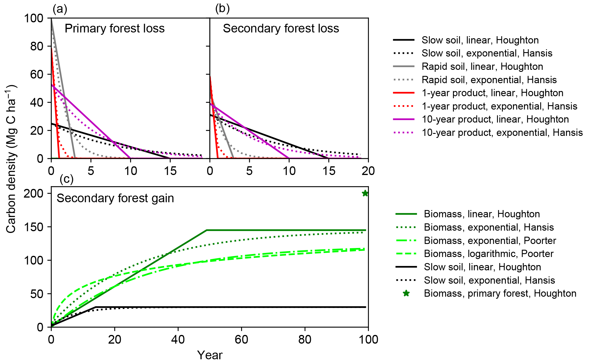
Figure 1 Response curves for tropical moist forest in bookkeeping models and from a recent field study. Solid and dotted lines indicate the linear (Houghton, 1999) and exponential (Hansis et al., 2015) curves respectively. Lime dashed and dash-dotted lines are the logarithmic and exponential curves from forest plots (Poorter et al., 2016). Vegetation carbon density in primary forest (Houghton, 1999) is also shown as a star in panel (c) for comparison.

2 Methods

The LULCCs considered in this study are forest loss (tropical moist forest transformed to cropland) and forest gain (cropland abandonment to secondary tropical moist forest) in Latin America. We construct a bookkeeping model to simulate the carbon balance of simultaneous forest loss and gain in the same region. This model is similar to those developed by Houghton  (1999) and Hansis et al. (2015) for global applications. After forest area loss, carbon density changes are calculated for biomass, two soil organic carbon pools (rapid and slow) and two product pools with turnover times of 1 and 10 years respectively. After the establishment of a secondary forest, carbon density changes in biomass and soil pools are considered. Only one slow soil pool is used in the regrowth of secondary forest, similar to Houghton (1999) and Hansis et al. (2015).

Both the linear response curves from Houghton (1999) and the exponential ones from Hansis et al. (2015) are used to simulate the dynamics of each carbon pool consecutive to initial LULCC (Fig. 1). For regrowing secondary forest, we also used two curves for biomass recovery based on a collection of field measurements by Poorter et al. (2016). The first one is a logarithmic equation describing aboveground biomass carbon as a function of stand age from Poorter et al. (2016), the parameters of which are derived using the average aboveground biomass recovery from multiple stands after 20 years. It should be noted that with a logarithmic curve, no asymptotic value is reached even after an infinite time, which is not realistic for estimating long-term budgets, as it would mean permanent carbon gains. To overcome this problem of the logarithmic curve, we define a fixed time horizon of 100 years after LULCC at which biomass becomes constant. The second biomass carbon gain curve is an exponential curve obtained by fitting the data from Poorter et al. (2016) with a saturating exponential function like in Hansis et al. (2015). This equation avoids the infinite increase in biomass after LULCC in the logarithmic curve. For both response curves, a ratio of 0.81 (Liu et al., 2015; Peacock et al., 2007; Saatchi et al., 2011) is used to convert aboveground biomass reported by Poorter et al. (2016) to total biomass, and this ratio is consistent with the one (0.82) that Poorter et al. (2016) used based on a FAO Forest Resources Assessment report (FAO, 2010).

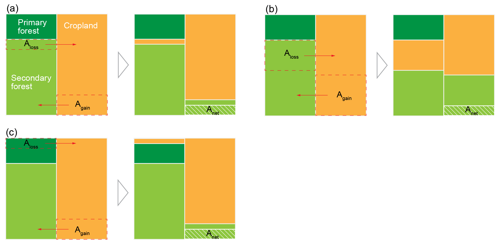
Figure 2 An illustration of different gross forest area changes with the same net area change. (a) Net forest gain with small gross secondary forest area changes (secondary to secondary), thus low ${\mathit{\gamma }}_{A_{\mathrm{net}}}^{A_{\mathrm{gross}}}$. (b) Same net forest gain as panel (a) but with large gross secondary forest area changes (secondary to secondary), thus high ${\mathit{\gamma }}_{A_{\mathrm{net}}}^{A_{\mathrm{gross}}}$. (c) Same as panel (a) but with gross primary forest loss (primary to secondary) instead of gross secondary loss.

To model the sensitivity of the carbon balance of a typical region in Latin America to different ratios of gross to net forest area change during initial pulse of forest area change followed by no change in forest area, we construct five idealized scenarios (Table 1). These scenarios are (i) S0 with no net but gross area changes, (ii) S1 with a net forest area loss being the sum of small gross area changes, (iii) S2 with the same net forest area loss as S1 but being a sum of large gross area changes, and (iv) S3 and (v) S4, similar to S1 and S2 but with a net forest area gain instead of a net loss. An example of small versus large gross area changes with the same net area change is illustrated in Fig. 2.

Table 1 Illustrative scenarios with different ratios of gross to net forest area changes impacting legacy LULCC emissions after a pulse disturbance of forest area at t = 0. A_net, A_gross, A_loss, A_gain and ${\mathit{\gamma }}_{A_{\mathrm{net}}}^{A_{\mathrm{gross}}}$ are the applied net forest area change, gross forest area change, gross forest loss area, gross forest gain area and the ratio of A_gross to A_net at t = 0. A positive value of an area change is an increase in forest area.

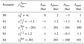
In each scenario, LULCC is applied as a pulse of forest area change at time t = 0, and we evaluate carbon changes over the following 100 years. The parameter ${\mathit{\gamma }}_{A_{\mathrm{net}}}^{A_{\mathrm{gross}}}$ is the ratio of gross forest change area (A_gross) to net forest change area (A_net) applied at t = 0.

$$\begin{array}{}\text{(1)}& {\mathit{\gamma }}_{A_{\mathrm{net}}}^{A_{\mathrm{gross}}}={\displaystyle \frac{A_{\mathrm{gross}}}{A_{\mathrm{net}}}},\end{array}$$

where

$$\begin{array}{}\text{(2)}& {\displaystyle }& {\displaystyle }{A}_{\mathrm{gross}}=\mathrm{|}{A}_{\mathrm{loss}}\mathrm{|}+A_{\mathrm{gain}}\text{(3)}& {\displaystyle }& {\displaystyle }{A}_{\mathrm{net}}=A_{\mathrm{loss}}+A_{\mathrm{gain}}.\end{array}$$

By convention, A_loss (< 0) and A_gain (> 0) are the gross forest loss and gain areas applied at t = 0. A positive value of A_net is an increase in forest area. For instance, the illustrative scenario S3 described in Table 1 explores the effects of a large positive value of ${\mathit{\gamma }}_{A_{\mathrm{net}}}^{A_{\mathrm{gross}}}$ on E_LULCC. E_LULCC is then simulated for contrasting A_gross and A_net transitions with the bookkeeping model as the sum of changes in all carbon pools over the area that was disturbed at t = 0. ΣE_LULCC,net is the cumulative LULCC carbon flux up to a time horizon t, calculated using only net area changes (A_net) and ignoring gross area changes. ΣE_LULCC,gross is the cumulative carbon flux using gross forest area change, which has two component fluxes: the cumulative emissions (ΣE_LULCC,loss) from gross forest loss and the carbon sink (ΣE_LULCC,gain) from secondary forest regrowth. This is calculated using

$$\begin{array}{}\text{(4)}& {\displaystyle }& {\displaystyle }\sum E_{\mathrm{LUC},\mathrm{gross}}=\sum E_{\mathrm{LUC},\mathrm{loss}}+\sum E_{\mathrm{LUC},\mathrm{gain}}\text{(5)}& {\displaystyle }& {\displaystyle }\sum E_{\mathrm{LUC},\mathrm{loss}}=-A_{\mathrm{loss}}\times L\left(t\right)\text{(6)}& {\displaystyle }& {\displaystyle }\sum E_{\mathrm{LUC},\mathrm{gain}}=A_{\mathrm{gain}}\times G\left(t\right),\end{array}$$

where L(t) and G(t) stand for the cumulative carbon density change in all carbon pools up to time t. Positive values of carbon fluxes indicate a loss of land carbon to the atmosphere.

Table 2 Different combinations of response curves to calculate E_LULCC.

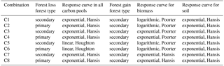
For each scenario in Table 1, we test different loss and gain response curves in our bookkeeping model, namely, linear or exponential carbon loss and linear, logarithmic or exponential increase for forest gain. In the case of gross forest area loss, we considered two options, either a primary forest (primary to secondary) or a secondary forest (secondary to secondary) being cleared (Table 2; also see an illustration in Fig. 2). This gives a total of eight combinations (C1 to C8 in Table 2) to calculate legacy E_LULCC after a forest area disturbance. Note that one basic principle of bookkeeping models is that the same equilibrium vegetation carbon density is assumed between a secondary forest being lost and a secondary forest having fully recovered. Therefore, the equilibrium biomass density of secondary forest being lost at t = 0 in C1, C3 and C5 is set to be the same as that of the fully recovered (100 years) secondary forest in Poorter et al. (2016).

We use Global Forest Change data from Hansen et al. (2013) to apply our conceptual calculation to the real-world gross and net forest changes. Forest cover data from Hansen et al. (2013) comprise three layers at 30 m resolution: tree cover fraction (0–100 % in each pixel) in the year 2000, forest area loss (each pixel labelled with a loss year) during 2000–2012 and forest gain during 2000–2012 (not specifying the gain year). As noted in Hansen et al. (2013), attributing the forest gain to a specific year is challenging because of the difficulty in detecting young forests from satellite reflectance measurements. In this study, we use the forest loss and forest gain layers to calculate the ratios of gross to net area changes (${\mathit{\gamma }}_{A_{\mathrm{net}}}^{A_{\mathrm{gross}}}$) at a 0.5^∘ × 0.5^∘ resolution, and thus ${\mathit{\gamma }}_{A_{\mathrm{net}}}^{A_{\mathrm{gross}}}$ represents the average values during 2000–2012 rather than for a single year since the year of forest gain is not reported. The gross changes at the 0.5^∘ level are calculated by summing the absolute areas of forest loss and gain at the 30 m level during 2000–2012 in each 0.5^∘ × 0.5^∘ grid cell, while the net changes are the sum of gross forest loss (negative) and gross forest gain (positive).

3 Results

3.1 Response curves and comparison with field measurements

The response curves of tropical moist forest from bookkeeping models of Houghton (1999) and Hansis et al. (2015) and from Poorter et al. (2016) for Latin America used in this study (Sect. 2) are displayed in Fig. 1. The curves of Houghton (1999) (linear) and Hansis et al. (2015) (exponential) are similar (Fig. 1) because the parameters of the exponential function were calibrated from the linear one (Hansis et al., 2015). Due to the higher carbon density of primary compared to secondary forest and the identical time at which both loss curves reach zero in Houghton (1999) and Hansis et al. (2015), the loss curves for a cleared primary forest are steeper than those for a cleared secondary forest (Fig. 1a, b). This implies that clearing a primary forest instead of a secondary one leads to larger legacy emissions. The fast decay of the rapid soil carbon pool in Fig. 1a and 1b is due to the fact that a fraction of the initial biomass is assigned to this pool after forest clearing (Hansis et al., 2015; Houghton, 1999).

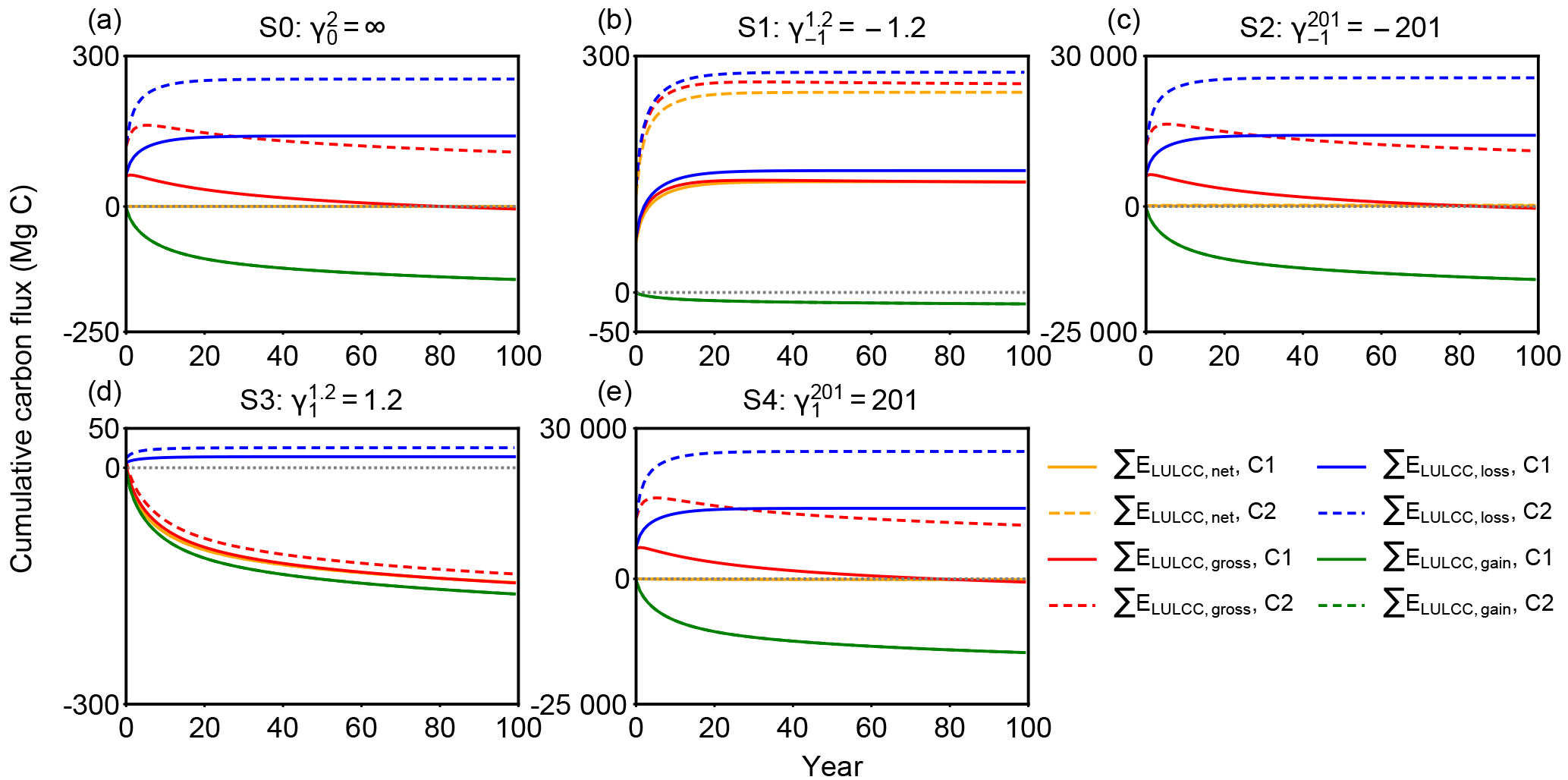
Figure 3 Cumulative carbon flux (ΣE_LULCC) after an initial forest area change at t = 0 followed by no change in forest area for the different scenarios S0 to S4 in Table 1 with different net and gross initial forest area changes. The response curves used in those bookkeeping model simulations are C1 in solid lines (Table 2) with a secondary-to-secondary forest change at t = 0 and a logarithmic biomass recovery curve with an asymptote, and C2 in dashed lines (primary-to-secondary forest change at t = 0 and a logarithmic biomass recovery curve with an asymptote). The dotted line is the zero line. A positive value of carbon flux indicates carbon emission to the atmosphere.

The logarithmic recovery curve (lime dashed lines in Fig. 1c) from Poorter et al. (2016) has an initial faster biomass growth rate of up to 20 years than in the curves used in previous bookkeeping models. After 20 or 30 years, however, the recovery curves of Houghton (1999) and Hansis et al. (2015) surpass the one of Poorter et al. (2016), leading to a higher equilibrium biomass of mature secondary forests (Fig. 1c). More precisely, the 100-year biomass of a secondary forest in Houghton (1999) and Hansis et al. (2015) is ≈ 25 % higher than in Poorter et al. (2016). The median time to recover 90 % of the maximum biomass is 66 years in Poorter et al. (2016), compared to only 44 years in Houghton (1999) and 55 years in Hansis et al. (2015) (Fig. 1c). The exponential recovery curve fit to the data from Poorter et al. (2016) (lime dash-dotted line in Fig. 1c) has lower biomass than the logarithmic curve in the first 40 years but reaches a similar density after 100 years (by construction). The exponential curve from Poorter et al. (2016) agrees well with the linear curve of Houghton (1999) during the first 20 years (Fig. 1c).

3.2 Temporal change of cumulative carbon fluxes in different LULCC scenarios

We calculated cumulative carbon fluxes for the five idealized forest area change scenarios (Table 1) with the eight combinations of response curves (Table 2), giving an ensemble of 40 simulations. Results for each simulation are shown in Fig. S1 in the Supplement. Here we compare the response curve combination C1 (exponential secondary forest loss and logarithmic biomass recovery) and C2 (exponential primary forest loss and logarithmic biomass recovery) as examples in Fig. 3 (see annual fluxes in Fig. S2) to illustrate the effect of different gross forest area change with the same net area change on cumulative carbon flux, i.e. the impact of ${\mathit{\gamma }}_{A_{\mathrm{net}}}^{A_{\mathrm{gross}}}$ on the E_LULCC. Other combinations provide conclusions similar to C1 and C2. For example, E_LULCC for C5 and C6 using linear curves for forest loss are very similar to C1 and C2 in Fig. S1.

In the scenario S0 with initial secondary forests and no net forest area change, ΣE_LULCC,net is zero when calculated based on net area change (Fig. 3a) but the gross carbon flux (ΣE_LULCC,gross) is distinct from zero. In the variant of the S0 scenario with initial primary forest (C2), due to the lower equilibrium carbon density of the secondary forest, ΣE_LULCC,gross is a large source after 100 years (red dashed lines in Fig. 3a). In the secondary forest loss and gain case (C1), ΣE_LULCC,gross is a carbon source in the initial period and gradually becomes carbon neutral with the compensation effects of secondary forest regrowth (red solid lines in Fig. 3a).

Both S1 and S2 scenarios have the same net forest area loss ($A_{\mathrm{net}}=-\mathrm{1}$ ha) but different gross forest area changes (${\mathit{\gamma }}_{-\mathrm{1}}^{\mathrm{1.2}}$ = −1.2 and ${\mathit{\gamma }}_{-\mathrm{1}}^{\mathrm{201}}$ = −201 for S1 and S2 respectively; Table 1). In S1 with a small gross area change (A_gross = 1.2 ha), ΣE_LULCC,gross is close to ΣE_LULCC,net (Fig. 3b), starting with either primary and secondary initial forests. By contrast, the difference between ΣE_LULCC,gross and ΣE_LULCC,net in S2 is large and positive, indicating a cumulative carbon loss much higher than S1 due to its large gross area change (Fig. 3c).

Scenario S3 versus scenario S4 with a net forest gain (A_net = +1 ha) but different ratios of gross to net area changes (${\mathit{\gamma }}_{A_{\mathrm{net}}}^{A_{\mathrm{gross}}}$) present a similar behaviour as S1 versus S2. However, the sign of ΣE_LULCC,gross is reversed, from a sink in S3 (red lines in Fig. 3d) to a source in S4 (red lines in Fig. 3e). Especially for the gross primary forest loss, ΣE_LULCC,gross exhibits a large source even after 100 years (red dashed lines in Fig. 3d, e). This implies that despite the net initial forest gain, the rate of gross area change determines the sign of ΣE_LULCC over a certain time horizon after the pulse of forest area change. More generally, this shows that, while long-term cumulative land-use change emissions are determined only by the net land-use area change (e.g. Gasser and Ciais, 2013), short-term cumulative emissions are determined by the gross area change.

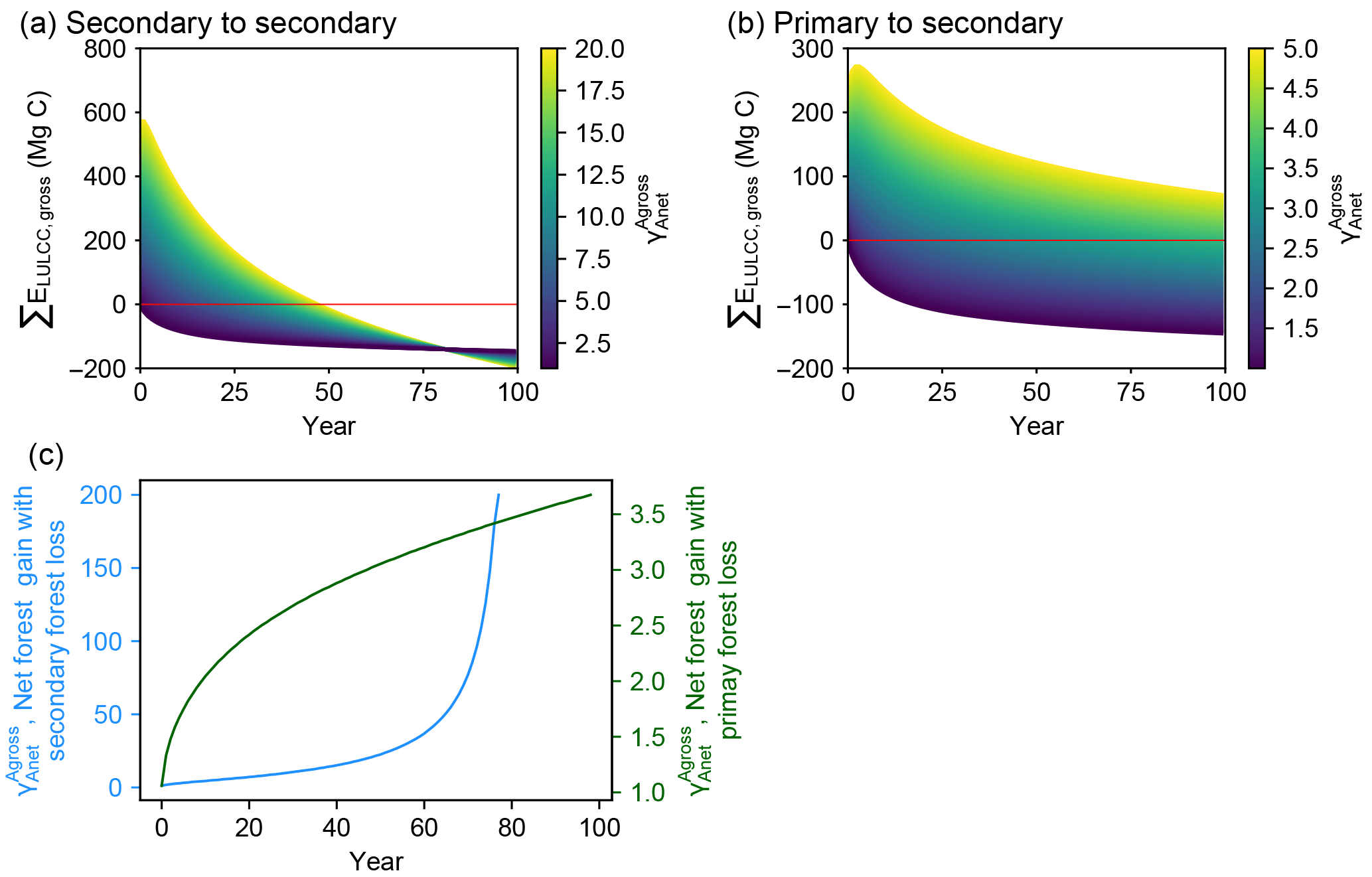
Figure 4 Time evolution of cumulative carbon flux (ΣE_LULCC,_gross) after an initial forest area change involving gross forest area changes followed by no forest area change. The three panels show results of our bookkeeping model for three case studies. (a) A net forest gain at t = 0 with initial secondary forest loss followed by secondary forest regrowth (secondary to secondary; C1 in Table 2), (b) the same net area gain at t = 0 with initial primary forest loss followed by secondary forest regrowth (primary to secondary; C2 in Table 2) and (c) the critical value of ${\mathit{\gamma }}_{A_{\mathrm{net}}}^{A_{\mathrm{gross}}}$ at which ΣE_LULCC,gross is zero, going from a net source to a net sink for a different time horizon on the x axis. The coloured curves in panels (a) and (b) have the same net area change (A_net = +1 ha) at t = 0 but variable values of the initial gross-to-net area change ratios (${\mathit{\gamma }}_{A_{\mathrm{net}}}^{A_{\mathrm{gross}}}$). The red line in panels (a) and (b) is the zero line, defining the time after initial forest area change at which the system reaches a neutral carbon balance. The blue and green lines in panel (c) represent the critical ratios for a net initial forest gain scenario with secondary-to-secondary (a) and primary-to-secondary (b) gross forest area change respectively. Values larger than this critical value indicate that the initial forest area change has the net effect to emit CO₂ for a given time horizon on the x axis. An exponential curve from Hansis et al. (2015) for carbon loss in all pools and gain in soil pool and a logarithmic curve from Poorter et al. (2016) for gain in biomass pool are used in this example (Table 2).

3.3 Change of ΣE_LULCC,gross with the same net forest gain but different gross area changes

The comparison of ΣE_LULCC,gross (Fig. 3) for the idealized scenarios (Table 1) illustrates the fact that different values of ${\mathit{\gamma }}_{A_{\mathrm{net}}}^{A_{\mathrm{gross}}}$ have a large impact on the magnitude and the sign of cumulative LULCC emissions depending on the time elapsed after the initial pulse of forest area change. We thus calculated the difference between ΣE_LULCC,gross and ΣE_LULCC,net by varying ${\mathit{\gamma }}_{A_{\mathrm{net}}}^{A_{\mathrm{gross}}}$ in a systematic manner in a net forest gain scenario (Fig. 4).

When ${\mathit{\gamma }}_{A_{\mathrm{net}}}^{A_{\mathrm{gross}}}$ is increased, i.e. with more forest land turnover at t = 0 for the same initial net forest area gain (A_net = +1 ha), the time for ΣE_LULCC,gross to become a net carbon sink becomes longer (Fig. 4a). With initial primary forest being cut at t = 0, the cumulative LULCC carbon flux is still a source of CO₂ to the atmosphere after 100 years, even in simulations in which the net forest area was increased at t = 0 (Fig. 4b). This highlights that the different initial carbon density of primary forest from secondary forest can lead to very long-term legacy emissions.

The critical value of ${\mathit{\gamma }}_{A_{\mathrm{net}}}^{A_{\mathrm{gross}}}$ that reverses the sign of ΣE_LULCC,gross from carbon source to sink increases as a function of the time horizon considered after the initial forest area change (Fig. 4c). The two cases with initial secondary and primary forest loss show a different trajectory of this ratio along time. In the former, ${\mathit{\gamma }}_{A_{\mathrm{net}}}^{A_{\mathrm{gross}}}$ increases slowly in the beginning and then sharply, while in the latter ${\mathit{\gamma }}_{A_{\mathrm{net}}}^{A_{\mathrm{gross}}}$ increases quickly at the initial stage and then at a smaller rate. In fact, if ΣE_LULCC,gross can reach zero (the point of sign change, let ΣE_LULCC,gross = 0), combining with Eqs. (1) to (6), the critical value of ${\mathit{\gamma }}_{A_{\mathrm{net}}}^{A_{\mathrm{gross}}}$ can be expressed as

$$\begin{array}{}\text{(7)}& {\mathit{\gamma }}_{A_{\mathrm{net}}}^{A_{\mathrm{gross}}}={\displaystyle \frac{L\left(t\right)-G\left(t\right)}{L\left(t\right)+G\left(t\right)}}.\end{array}$$

This critical value of ${\mathit{\gamma }}_{A_{\mathrm{net}}}^{A_{\mathrm{gross}}}$ is independent of the initial forest area but determined by the carbon density changes at a given time consecutive to a change of forest area. Thus, for a secondary forest loss and gain at t = 0, the long-term L(t) + G(t) tends to zero and ${\mathit{\gamma }}_{A_{\mathrm{net}}}^{A_{\mathrm{gross}}}$ goes to infinite. For a primary forest loss and secondary forest gain at t = 0, the long-term L(t) + G(t) is the difference in the equilibrium carbon densities between primary and secondary forest, and therefore ${\mathit{\gamma }}_{A_{\mathrm{net}}}^{A_{\mathrm{gross}}}$ approaches a constant value at t = infinite. Furthermore, it should be noted that our approach of analyzing the critical value of ${\mathit{\gamma }}_{A_{\mathrm{net}}}^{A_{\mathrm{gross}}}$ is not limited to net forest gain scenarios or to LULCC transitions between forest and cropland. The framework of ${\mathit{\gamma }}_{A_{\mathrm{net}}}^{A_{\mathrm{gross}}}$ can also be extended to other LULCC scenarios, including lower, higher and equal equilibrium biomass density between two land-use types. For example, if a regrowing forest can achieve a higher equilibrium carbon density than the initial one, there is also a critical ${\mathit{\gamma }}_{A_{\mathrm{net}}}^{A_{\mathrm{gross}}}$ for the net forest loss scenario, for which the gross carbon emission becomes a sink at a certain time after initial forest area change. This situation may happen in reality, if the deforested forests are replaced by more productive species or under active management like fertilization and irrigation. Even in the field measurements by Poorter et al. (2016), some neotropical secondary forests show very high biomass resilience, i.e. reaching to a higher biomass than pre-deforestation.

We also calculated the critical ratios over time based on the exponential biomass response curves from Hansis et al. (2015) in comparison with the response curves from Poorter et al. (2016) (Fig. S3). As shown in Fig. 1, the equilibrium of secondary forest vegetation density with the recovery curve of Hansis et al. (2015) is higher than with Poorter et al. (2016) and we assumed the same density of primary forest for both, and thus L_{Hansis,primary}(t) = L_{Poorter,primary}(t), L_{Hansis,secondary}(t) > L_{Poorter,secondary}(t) and G_Hansis(∞) > G_Poorter(∞). Note that a positive value of carbon flux indicates carbon emission to the atmosphere. Combined with Eq. (7), the different equilibrium states of secondary forest vegetation can explain the differences in critical ratios over time between Hansis et al. (2015) and Poorter et al. (2016) in Fig. S3.

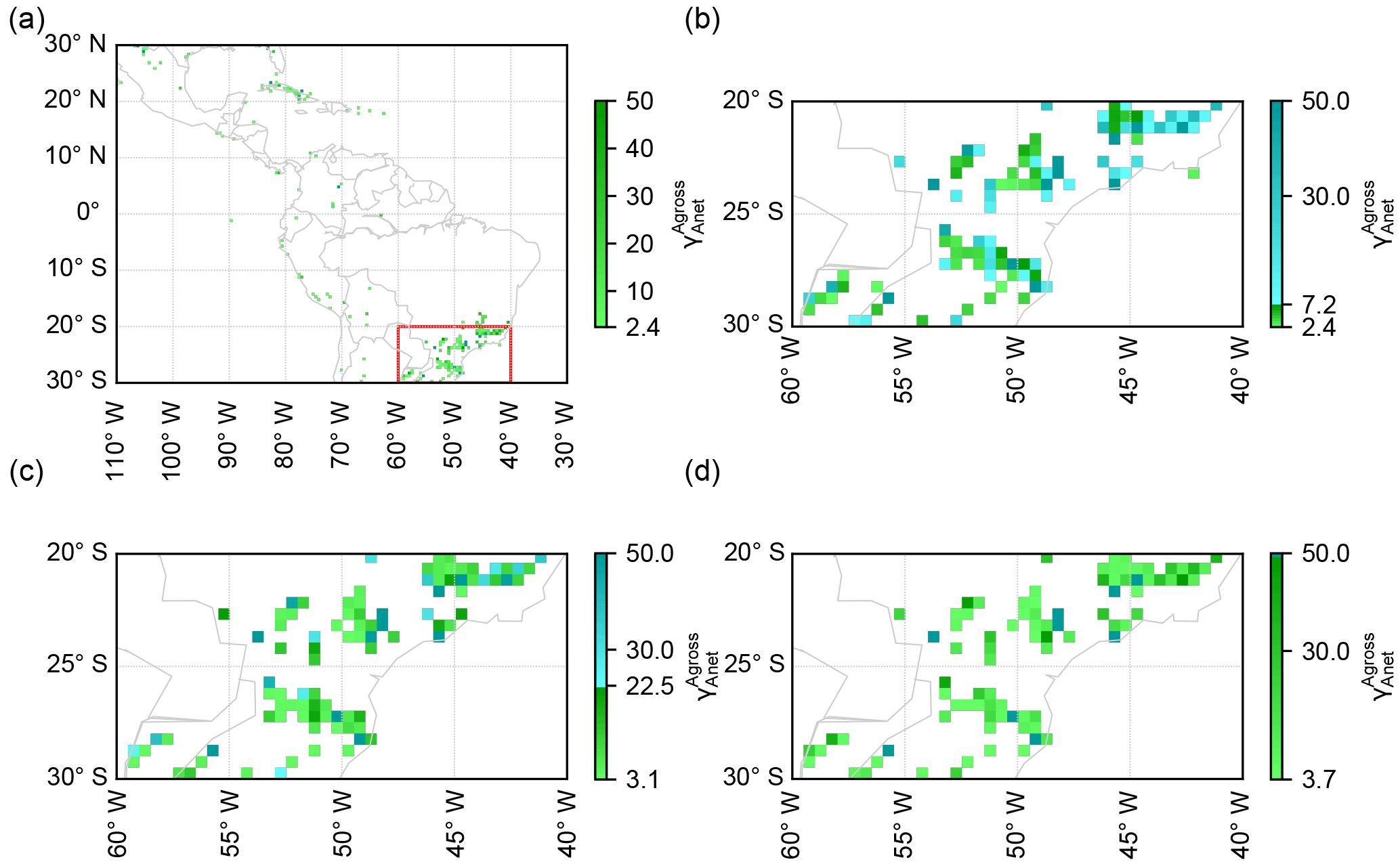
Figure 5 Ratios of gross to net forest area change (${\mathit{\gamma }}_{A_{\mathrm{net}}}^{A_{\mathrm{gross}}}$) in 0.5^∘ × 0.5^∘ grid cells in Latin America (same region as Poorter et al., 2016) calculated from the high-resolution forest cover change map (Hansen et al., 2013). Grid cells with ${\mathit{\gamma }}_{A_{\mathrm{net}}}^{A_{\mathrm{gross}}}$ < 2.4 are masked. Panel (b) is the zoom-in area of 20–30^∘ S and 40–60^∘ W in panel (a) (red rectangle) and grid cells with ${\mathit{\gamma }}_{A_{\mathrm{net}}}^{A_{\mathrm{gross}}}$ > 7.2 and with 2.4 < ${\mathit{\gamma }}_{A_{\mathrm{net}}}^{A_{\mathrm{gross}}}$ < 7.2 are shown as blue and green respectively to indicate those beyond the critical ratios with a time horizon of 20 years. Panels (c) and (d) are similar to panel (b) but indicate time horizons of 50 and 100 years respectively. The blue grid cells in panels (b) and (c) represent a cumulative carbon emission in 20 years no matter whether the lost forest is primary or secondary. The green grid cells in panels (b), (c) and (d) represent a cumulative carbon emission only if the cleared forests are primary forests.

3.4 Ratios in Latin America from satellite imagery

Based on the theoretical evidence for the existence of a critical value of the gross-to-net forest area change ratio (${\mathit{\gamma }}_{A_{\mathrm{net}}}^{A_{\mathrm{gross}}}$), which determines the sign and magnitude of ΣE_LULCC,gross at a given time after an initial net forest area change, we further combined such ratios with the land-cover change dataset to determine whether a region is a carbon sink or source at a given time horizon. Using the 30 m resolution forest area change data of Hansen et al. (2013) between 2000 and 2012, we calculated the ratios (${\mathit{\gamma }}_{A_{\mathrm{net}}}^{A_{\mathrm{gross}}}$) at a spatial resolution of 0.5^∘ × 0.5^∘ in the same region of Latin America as Poorter et al. (2016). The spatial resolution of 0.5^∘ × 0.5^∘ is a typical resolution of DGVMs when they simulate global E_LULCC. We set a future time horizon of 20 years as that is close to the targeted year in the nationally determined contributions (NDCs) (Grassi et al., 2017). From Fig. 4c, the critical values of ${\mathit{\gamma }}_{A_{\mathrm{net}}}^{A_{\mathrm{gross}}}$ at 20 years after an initial change in forest area are 7.2 and 2.4 respectively for secondary-to-secondary and primary-to-secondary initial transitions. For a longer time horizon of 50 years, the critical values are 22.5 and 3.1 respectively. After 100 years of the initial forest area change, while the critical value of ${\mathit{\gamma }}_{A_{\mathrm{net}}}^{A_{\mathrm{gross}}}$ for secondary-to-secondary transition goes to infinite, it approaches a constant value of 3.7 for primary-to-secondary forest change (Fig. 4c).

The map of ${\mathit{\gamma }}_{A_{\mathrm{net}}}^{A_{\mathrm{gross}}}$ diagnosed from the 30 m Landsat forest cover data in grid cells of 0.5^∘ × 0.5^∘ is shown in Fig. 5. Note that here we focus only on the grid cells with a net forest gain. The number of 0.5^∘ × 0.5^∘ grid cells in which ${\mathit{\gamma }}_{A_{\mathrm{net}}}^{A_{\mathrm{gross}}}$ > 7.2, that is grid cells in which current forest area change will lead to a source of CO₂ over a 20-year horizon, is 102 in our domain (Fig. 5a), which accounts for 35 % of the total number of grid cells in which a net forest gain is observed between 2000 and 2012. In these 102 grid cells, the ΣE_LULCC,gross is simulated to be a cumulative carbon emission in 20 years, no matter whether the lost forest is primary or secondary. If primary forests are cleared in grid cells with 2.4 < ${\mathit{\gamma }}_{A_{\mathrm{net}}}^{A_{\mathrm{gross}}}$ < 7.2 (33 % of the total forest gain grid cells, Fig. 5a), the 20-year ΣE_LULCC,gross is also a carbon source rather than a sink. We note that it is not possible to separate the primary and secondary forest in the forest cover data of Hansen et al. (2013). Thus, we cannot say whether these grid cells with 2.4 < ${\mathit{\gamma }}_{A_{\mathrm{net}}}^{A_{\mathrm{gross}}}$ < 7.2 are a carbon source or sink in the real world. For a time horizon of 50 years, the fractions of grid cells with ${\mathit{\gamma }}_{A_{\mathrm{net}}}^{A_{\mathrm{gross}}}$ > 22.5 and with 3.1 < ${\mathit{\gamma }}_{A_{\mathrm{net}}}^{A_{\mathrm{gross}}}$ < 22.5 in total net forest gain grid cells are 14 and 46 % respectively (Fig. 5c). The 100-year ΣE_LULCC,gross in grid cells with ${\mathit{\gamma }}_{A_{\mathrm{net}}}^{A_{\mathrm{gross}}}$ > 3.7 (53 % of total) is also possibly a carbon source if lost forest is primary in these grid cells (Fig. 5d). The grid cells with ${\mathit{\gamma }}_{A_{\mathrm{net}}}^{A_{\mathrm{gross}}}$ greater than the critical values are mainly distributed in southeastern Brazil (Fig. 5b, c, d).

By comparison, we also calculated the number of grid cells with ${\mathit{\gamma }}_{A_{\mathrm{net}}}^{A_{\mathrm{gross}}}$ above the critical ratio for the biomass response curves from Hansis et al. (2015) (Table S1). Because of the differences in the critical values of ${\mathit{\gamma }}_{A_{\mathrm{net}}}^{A_{\mathrm{gross}}}$ over time (Fig. S3) between curves from Poorter et al. (2016) and Hansis et al. (2015), a higher critical ratio leads to a smaller number of 0.5^∘ × 0.5^∘ grid cells with ${\mathit{\gamma }}_{A_{\mathrm{net}}}^{A_{\mathrm{gross}}}$ beyond the critical ratio (Table S1).

In addition to the number of grid cells with ${\mathit{\gamma }}_{A_{\mathrm{net}}}^{A_{\mathrm{gross}}}$ above the critical ratio, we further showed the differences between the cumulative carbon flux using gross transitions (ΣE_LULCC,gross) and net transitions (ΣE_LULCC,net) in these grid cells (Table S2). Taking C1 (secondary to secondary) at a 20-year horizon for example, using net transitions results in a carbon sink of 12 Tg C, but using gross transitions results in a carbon emission of 21 Tg C (Table S2) in the grid cells with ${\mathit{\gamma }}_{A_{\mathrm{net}}}^{A_{\mathrm{gross}}}$ > 7.2 (Fig. 5b).

4 Discussion

The biomass recovery curves of neotropical secondary forests from Poorter et al. (2016) are lower 20 years after the initial perturbation than those used in the bookkeeping models of Houghton (1999) and Hansis et al. (2015), implying that these models simulate different LULCC carbon fluxes in Latin America from those using the recovery curves of Poorter et al. (2016). The carbon density in undisturbed forests in the bookkeeping models of Houghton (1999) and Hansis et al. (2015) was essentially based on Whittaker and Likens (1973), multiplied by a factor of 0.75 to approximate the lower carbon density of secondary forests (Houghton et al., 1983). The carbon density data from Whittaker and Likens (1973) are subject to two sources of uncertainty. First, these values represent biomass in the 1950s (Woodwell et al., 1978) rather than present day, and second, they were compiled from very limited field measurements for tropical forests. In fact, Whittaker and Likens (1973) claimed in their study that data “for tropical communities are very meager” and the mean biomass density is “a subjectively chosen intermediate value based on very few measurements” to avoid extreme values.

Differences may also exist for soil carbon dynamics after LULCC. There are a great number of meta-analyses or reviews (Conant et al., 2001; Davidson and Ackerman, 1993; Davis and Condron, 2002; Don et al., 2011; Guo and Gifford, 2002; Kurganova et al., 2014; Laganière et al., 2010; Li et al., 2012; Marín-Spiotta and Sharma, 2013; Murty et al., 2002; Paul et al., 2002; Poeplau et al., 2011; Post and Kwon, 2000; Powers et al., 2011; Wei et al., 2014; West et al., 2004) on the soil organic carbon change after LULCC based on field measurement data (mostly paired sites and chronosequences). These studies may generally agree on the directions of soil carbon change after LULCC (e.g. soil carbon loss after forest clearing for cropland), but the magnitudes and temporal dynamics of soil carbon changes remain highly uncertain because, among other things, of the limited site number and the diversity of soil properties. Field measurements at site level may be unrepresentative of the whole region because the distribution of biophysical conditions like soil texture, precipitation and temperature may not match the distribution of the whole set of such factors in the LULCC areas in a given region (Powers et al., 2011).

Some DGVMs (Bayer et al., 2017; Shevliakova et al., 2009; Stocker et al., 2014; Wilkenskjeld et al., 2014; Yue et al., 2017) as well as a bookkeeping model (Hansis et al., 2015) have implemented gross land-use and land-cover transitions, and thus simulated a higher E_LULCC than using only net transitions. Arneth et al. (2017) reviewed the “missing processes” in LULCC modelling with DGVMs and found that ignoring gross LULCC could underestimate the global ΣE_LULCC by 36 Pg C on average over the historical period (1901–2014). In this study, we used a bookkeeping method to quantify the difference in LULCC emissions calculated using net versus gross forest area transitions and to show the existence of critical ratios of gross to net forest area changes above which land-use action will cause a reversed sign of cumulative carbon flux. Evidently, the choice of a time horizon to assess the carbon balance of a system after an initial pulse of forest area change influences the value of the critical ratio ${\mathit{\gamma }}_{A_{\mathrm{net}}}^{A_{\mathrm{gross}}}$. The desirable target time lengths could be different depending on specific mitigation projects or land-use reduction policies, and thus critical values of the gross-to-net forest area change ratio are different (Fig. 4c). Conversely, because of the temporal evolution of legacy carbon fluxes after initial land disturbance, it is important to define a specific and reasonable time horizon when making land-based mitigation policies.

As a conceptual analysis, the assumptions we made raise uncertainties. First, the logarithmic biomass recovery curve adopted in Poorter et al. (2016) does not seem to be appropriate for LULCC carbon emission modelling because it will not reach an equilibrium state. We thus fitted the data from Poorter et al. (2016) with an exponential saturating curve to avoid this issue. Second, we used a median biomass recovery rate for the whole tropical moist forest region in Latin America. In reality, however, due to the different climate, soils and other ecosystem conditions, recovery rates vary, and thus spatially explicit recovery rates should better depict regional patterns of secondary forest regrowth and net LULCC emissions. In the dry tropics, the critical ratio values may be smaller because of the slower biomass recovery rates. Third, the biomass and soil carbon densities in initial vegetation and the equilibrium vegetation after LULCC are also spatially different in the real world. The distinction between primary and secondary forest being lost at t = 0 is a typical example of how different initial carbon density impacts the legacy LULCC carbon flux and thus the determined critical gross-to-net forest area change ratio values. In fact, a large spatial gradient of biomass exists from the northeastern to southwestern Amazon regions (Saatchi et al., 2007, 2011). One possible approach to account for the spatial variations in both biomass recovery rate and biomass density would be to reconstruct spatially explicit biomass–age curves using the relationship between regrowth rates and climate (Poorter et al., 2016) and to combine them with observation-based biomass densities (Baccini et al., 2012; Saatchi et al., 2011) and satellite-based forest cover change (Hansen et al., 2013). However, uncertainties arise in the up-scaling of biomass recovery rates and lack of information on annually resolved forest gain from Hansen et al. (2013). In addition, spatially explicit soil carbon density maps are also uncertain.

The effect of gross versus net forest area change on legacy LULCC emissions certainly differs across forest ecosystems and other LULCC transition types (e.g. transitions between grassland and cropland). The concept of critical ratios of gross to net LULCC affecting legacy carbon balance can be extended in other regions where forest management practice is critical (e.g. North America and Europe). Forest management practices like wood harvest and thinning extract carbon from the ecosystem and release it to the atmosphere (Houghton et al., 2012), while recovering secondary forest from past deforestation and logging (Pan et al., 2011) and even old-growth forests (Luyssaert et al., 2012) can act as carbon sinks. In theory, likewise, a critical ratio value should exist to balance the bidirectional carbon fluxes in forest management practices. An advantage of this concept of critical ratio is that it can be directly measured with satellite observations, which provides a quick guide for local land-use management practice through near-real-time forest cover change data (e.g. Global Forest Watch, http://www.globalforestwatch.org/).

Accurate estimates of LULCC carbon fluxes in the neotropical forests are increasingly important for climate mitigation policy with the progressive implementation of Reducing Emissions from Deforestation and forest Degradation (REDD+) programs under the United Nations Framework Convention on Climate Change (UNFCCC) (Angelsen et al., 2009; Magnago et al., 2015). Furthermore, forest-based climate mitigation has been taken as a key option in the nationally determined contributions proposed by some countries to the Paris Climate Agreement, accounting for about one-fourth of total intended emission reductions from a predefined baseline (Grassi et al., 2017). Brazil contributes about one-third of the global forest-based emission reduction in the NDCs (Grassi et al., 2017). Based on the results of this study, we argue that it will be important to carefully distinguish the amount of gross vs. net forest changes and clearing of primary vs. secondary forest when assessing national forest-based mitigation pledges. With a large gross-to-net area change ratio, a net forest gain could still lead to a net carbon source over a long period in the future. Our work has the potential to be extended to the country level and other LULCC types as long as information on vegetation and soil carbon densities changes after LULCC is available, and a critical value of ${\mathit{\gamma }}_{A_{\mathrm{net}}}^{A_{\mathrm{gross}}}$ can be estimated as a guideline to evaluate land-based mitigation policies for each region. More observation-based data on land-use area change and carbon loss and gain curves will definitely help to extend the range of applications of the critical gross-to-net area ratio concept.

5 Conclusions

Using only net LULCC transitions instead of gross values can bias the magnitude of estimated LULCC carbon fluxes, to the point of estimating a sink instead of a source in reality if high gross forest area change occurs. We used idealized scenarios to demonstrate different aspects of the discrepancy between net and gross forest changes, defining the ${\mathit{\gamma }}_{A_{\mathrm{net}}}^{A_{\mathrm{gross}}}$ metric as the ratio of gross area change to net area change. Our S0 experiment even shows that there is no net forest change; LULCC may actually lead to a carbon source, depending on the gross forest change area. S1 and S2 show that with the same net forest loss, different ratios of gross to net forest change (${\mathit{\gamma }}_{A_{\mathrm{net}}}^{A_{\mathrm{gross}}}$) alter the magnitude of differences between net and gross cumulative carbon fluxes. Similarly, S3 and S4 show that with the same amount of net forest gain area, different ${\mathit{\gamma }}_{A_{\mathrm{net}}}^{A_{\mathrm{gross}}}$ can even change the directions of carbon fluxes, i.e. from a gross carbon sink to source even that net forest area increases. We further determined the critical ratios in net forest gain grid cells (${\mathit{\gamma }}_{A_{\mathrm{net}}}^{A_{\mathrm{gross}}}$ = 7.2 and 2.4 respectively for secondary and primary forest clearing), above which the gross cumulative carbon fluxes show a sign reversed from the net ones at 20 years after LULCC occurred. These analyses reveal the importance of using gross LULCC transitions rather than net LULCC transitions in both bookkeeping models and DGVMs. The concept of critical ratio can also be implemented in other LULCC transitions in other regions and used as a guide for carbon balance estimation in forest management.