the Creative Commons Attribution 4.0 License.
the Creative Commons Attribution 4.0 License.
 | 29 Nov 2019
Regulation of N2O emissions from acid organic soil drained for agriculture
Arezoo Taghizadeh-Toosi
Lars Elsgaard
Tim J. Clough
Rodrigo Labouriau
Vibeke Ernstsen
Søren O. Petersen
Organic soils drained for crop production or grazing land are agroecosystems with potentially high but variable emissions of nitrous oxide (N2O). The present study investigated the regulation of N2O emissions in a raised bog area drained for agriculture, which is classified as potentially acid sulfate soil. We hypothesised that pyrite (FeS2) oxidation was a potential driver of N2O emissions through microbially mediated reduction of nitrate (). Two sites with rotational grass, and two sites with a potato crop, were equipped for monitoring of N2O emissions and soil N2O concentrations at the 5, 10, 20, 50 and 100 cm depth during weekly field campaigns in spring and autumn 2015. Further data acquisition included temperature, precipitation, soil moisture, water table (WT) depth, and soil and ammonium () concentrations. At all sites, the soil was acidic, with pH ranging from 4.7 to 5.4. Spring and autumn monitoring periods together represented between 152 and 174 d, with cumulative emissions of 4–5 kg N2O-N ha−1 at sites with rotational grass and 20–50 kg N2O-N ha−1 at sites with a potato crop. Equivalent soil gas-phase concentrations of N2O at grassland sites varied between 0 and 25 µL L−1 except for a sampling after slurry application at one of the sites in spring, with a maximum of 560 µL L−1 at the 1 m depth. At the two potato sites the levels of below-ground N2O concentrations ranged from 0.4 to 2270 µL L−1 and from 0.1 to 470 µL L−1, in accordance with the higher soil mineral N availability at arable sites. Statistical analyses using graphical models showed that soil N2O concentration in the capillary fringe (i.e. the soil volume above the water table influenced by tension saturation) was the strongest predictor of N2O emissions in spring and, for grassland sites, also in the autumn. For potato sites in autumn, there was evidence that availability in the topsoil and temperature were the main controls on N2O emissions. Chemical analyses of intact soil cores from the 0 to 1 m depth, collected at adjacent grassland and potato sites, showed that the total reduction capacity of the peat soil (assessed by cerium(IV) reduction) was much higher than that represented by FeS2, and the concentrations of total reactive iron (TRFe) were higher than those of FeS2. Based on the statistical graphical models and the tentative estimates of reduction capacities, FeS2 oxidation was unlikely to be important for N2O emissions. Instead, archaeal ammonia oxidation and either chemodenitrification or nitrifier denitrification were considered to be plausible pathways of N2O production in spring, whereas in the autumn heterotrophic denitrification may have been more important at arable sites.
- Article
(4869 KB) - Full-text XML
-
Supplement
(1120 KB) - BibTeX
- EndNote


Worldwide, 255 000 km2 of organic soils have been drained for agricultural use, mainly for cropland (Tubiello et al., 2016), and this accelerates decomposition of soil organic matter and net carbon (C) and nitrogen (N) mineralisation above the water table (WT; Schothorst, 1977). Drained organic soils are significant net sources of greenhouse gas (GHG) emissions as carbon dioxide (CO2) and nitrous oxide (N2O; Goldberg et al., 2010; Maljanen et al., 2003). A recent supplement to the “2006 IPCC Guidelines for National Greenhouse Gas Inventories on Wetlands” (IPCC, 2014) proposed average annual emission factors of 4.3 and 8.2 kg N2O-N ha−1 yr−1 for temperate grassland on drained organic soil with low and high nutrient status, respectively, and an emission factor of 13 kg N2O-N ha−1 yr−1 for cropland. For soil C losses, the emission factors proposed for these three land use categories were between 5.3 and 7.9 MgCO2-C ha−1 yr−1 (Hiraishi et al., 2014). Thus, while CO2 emissions are more important overall, site conditions appear to be more critical for N2O.
Site conditions are defined by land use, management, inherent soil properties and climate (Mander et al., 2010; Leppelt et al., 2014). Both WT drawdown (Aerts and Ludwig, 1997) and WT rise (Goldberg et al., 2010) may enhance N2O emissions, but such effects depend on soil N status (Martikainen et al., 1993; Aerts and Ludwig, 1997). Maljanen et al. (2003) found that WT, CO2 emissions and temperature at the 5 cm depth explained 55 % of the observed variability in N2O emissions during a 2-year field study on a drained organic soil, whereas the response to N fertilisation was limited, and they suggested that N released by soil organic matter mineralisation was the main source of N2O. In a study comparing GHG emissions from organic soil with different land uses in three regions of Denmark (in total eight site years), Petersen et al. (2012) also found that site conditions such as WT, pH and precipitation contributed significantly to explaining N2O emission dynamics. Among sites with arable crops in three regions, two sites had N2O emissions corresponding to, respectively, 38 and 61 kg N ha−1 yr−1; both of these sites showed distinct seasonal patterns, with the highest emissions in spring and autumn periods, whereas emissions at the third site were lower (6.4 kg N2O-N ha−1 yr−1) and much less variable. Notably, WT depth at the two sites with seasonal patterns of N2O emission fluctuated between 10–30 cm and 100–120 cm, whereas WT depth at the third site remained at 90–125 cm throughout the 14-month monitoring period.
Several processes can lead to N2O formation in acid organic soil: biotic processes include ammonia (NH3) oxidation to nitrite (NO2) by archaea or bacteria (Herrmann et al., 2012; Herold et al., 2012; Stieglmeier et al., 2014) as well as nitrifier denitrification and heterotrophic denitrification by bacteria or fungi (Liu et al., 2014; Maeda et al., 2015; Wrage-Mönnig et al., 2018). The recently discovered process comammox by Nitrospira sp. is also a potential, but probably minor, source of N2O (Kits et al., 2019; Palomo et al., 2019). Abiotic N2O production can occur through chemodenitrification (Van Cleemput and Samater, 1996; Jones et al., 2015) or abiotic codenitrification (Spott et al., 2011). The two regions showing extreme N2O emissions from arable soil had both developed from marine forelands and were categorised as potentially acid sulfate soil, i.e. saturated to poorly drained soil containing pyrite (FeS2) that, upon oxidation, may lead to acid production in excess of the soil's neutralising capacity (Madsen and Jensen, 1988). The capillary fringe of organic soils represents an interface between saturated and unsaturated soil conditions, in which the extent of tension saturation depends on pore size distribution (Gillham, 1984). Previously, it has been speculated that oxidation and reduction of iron sulfides could influence N transformations during periods with a changing groundwater level (Petersen et al., 2012). Drainage promotes oxidation of FeS2, a process which may be linked to microbially mediated nitrate () reduction (Jørgensen et al., 2009; Torrento et al., 2010). The complete reduction of to dinitrogen (N2) can proceed as follows:
However, in the capillary fringe, residual oxygen (O2), or, alternatively, the acidification produced by FeS2 oxidation, could favour incomplete denitrification with accumulation of the intermediate N2O (Torrento et al., 2010):
Nitrate reduction via the reaction described in Eq. (2) could potentially have contributed to the very high N2O emissions reported previously from two arable sites where groundwater sulfate concentrations were also consistently high (Petersen et al., 2012).
Here, we studied four agricultural sites within one of the regions previously investigated by Petersen et al. (2012), i.e. a raised bog area with acid soil conditions. This study included two sites with rotational grass and two sites with a potato crop, and monitoring took place in spring and autumn periods, where high emissions of N2O occurred in previous studies (Petersen et al., 2012; Kandel et al., 2018). We hypothesised that FeS2 oxidation coupled with reduction was a possible driver of N2O emissions. It was further hypothesised that N2O emissions would vary with site conditions affecting denitrification (mineral N availability, rainfall, WT depth and temperature).
2.1 Study sites
The sites investigated were located in Store Vildmose, which is a 5000 ha raised bog in northern Jutland, Denmark. The area was, until 150 years ago, the largest raised bog in Denmark and largely unaffected by human activity. The bog overlies a marine plain formed by the last marine transgression; the sea retreated at around 8000 BCE, and peat later developed in wet parts of the landscape, attaining a maximum depth of 4.5 to 5.3 m in central parts of the bog (Kristensen, 1945). Between 1880 and 2010, the peat has generally subsided by at least 2 m due to drainage for agriculture or peat excavation (Regina et al., 2016), and today the peat depth is mostly 1–2 m but is even less in some locations (Kandel et al., 2018). The peat and underlying sand are acidic and have been categorised as a potentially acid sulfate soil (Madsen and Jensen, 1988). According to Kandel et al. (2018), the peat at the 0–25 cm depth in arable soil in this area has a high degree of humification, which corresponds to H8 on the von Post scale.
Four sites were selected along an east–west transect (Fig. 1a). One arable site (AR1) was in a field cropped with second-year potato in 2015, while an adjacent site (RG1) in a neighbouring field had second-year rotational grass; these two sites were also represented in the study of Petersen et al. (2012) as N-AR and N-RG, respectively. Land use treatments (i.e. potato and rotational grass) were replicated at sites in other fields and will be referred to as AR2 and RG2. AR2 was located 4.6 km to the west, and RG2 was located 1.7 km to the east of the paired AR1–RG1 sites (Figs. 1a and S1 in the Supplement).
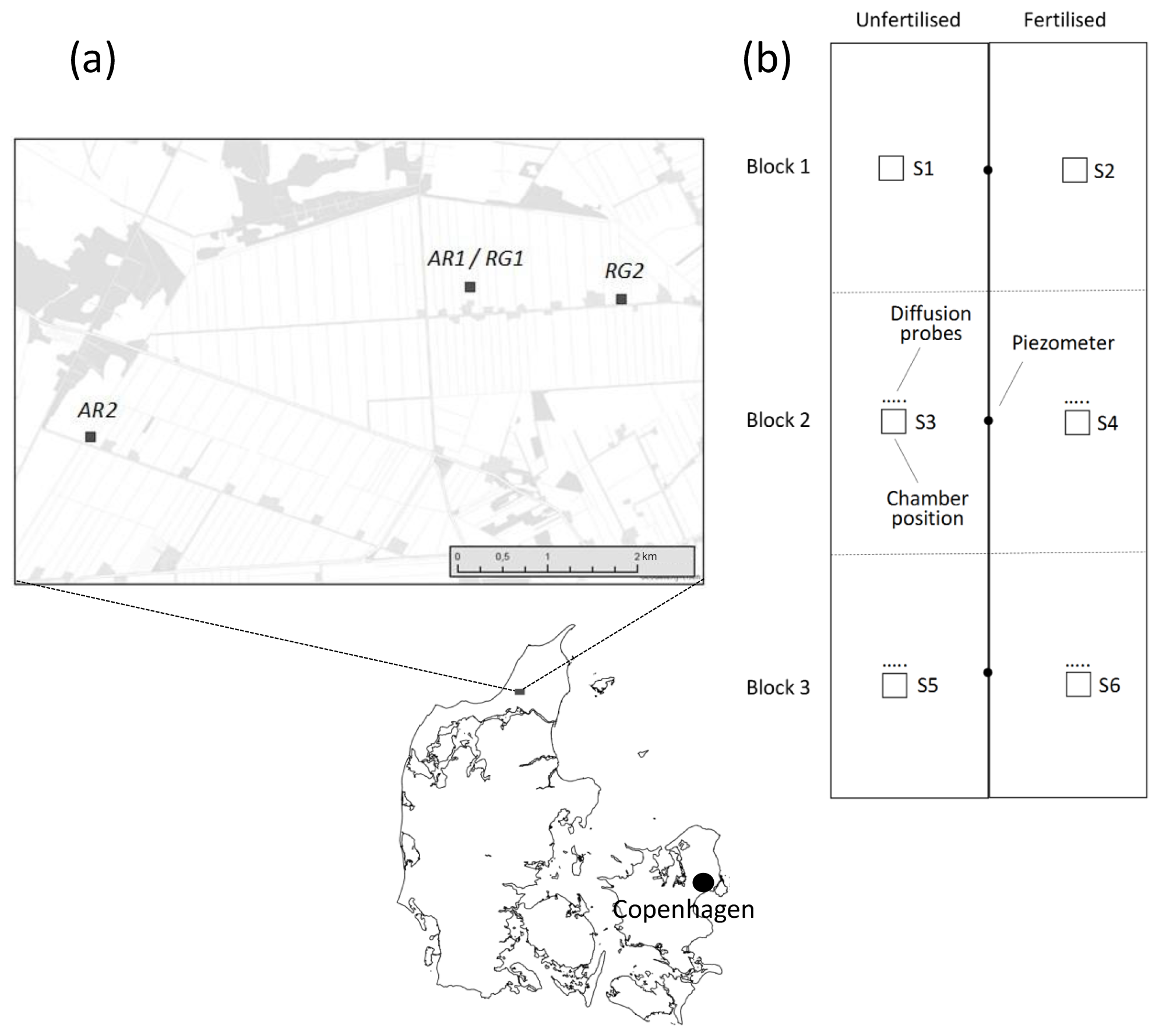
Figure 1(a) Location of AR1 and RG1 (both at 57∘13′59.7′′ N, 9∘50′40.3 E), RG2 (57∘13′55.9′′ N, 9∘52′20.2 E) and AR2 (57∘13′7.6′′ N, 9∘46′26.9 E). (b) Experimental design at each of the four sites, with three blocks cantered around piezometers (•) and two subplots, one of which received N fertiliser at the rate of the surrounding field. Six collars for gas flux measurements (Figs. S1–S6 in the Supplement) were distributed as indicated, and sets of five diffusion probes for soil gas sampling were installed near collars in selected positions (see text).
2.2 Experimental design
In January 2015, an area of 10 m × 24 m was selected at each site. Sampling positions were georeferenced using a Topcon HiPer SR geopositioning system (Livermore, CA). On 25 February 2015, each site was fenced, and three 10 m × 8 m experimental blocks were defined (Fig. 1b). Each site was further divided along its longitudinal axis to establish two 5 m × 24 m fertilisation subplots.
For monitoring of WT depth, piezometer tubes (Rotek A/S, Sønder Felding, Denmark) were installed to the 150 cm depth at the centre of each block. On either side of the piezometers, at 2.7 m distance, collars of white PVC (base area: 55 cm × 55 cm; height: 12 cm – RG – or 24 cm – AR) were installed at between the 5 and 10 cm depth (Fig. 1). The higher collars used at AR sites were level with the ridges established around potato rows during the growth period. The collars, which were fixed to the ground by four 40 cm pegs, had a 4 cm wide flange extending outwards at 2 cm from the top to support gas flux chambers. To prevent soil disturbance during gas sampling, platforms (60 cm × 100 cm) of perforated PVC were placed in front of each collar to create a boardwalk. The exact headspace of each collar was determined from 16 individual measurements of distance from the upper rim; this procedure was repeated whenever collars had been removed and reinstalled to accommodate field operations.
Sets of five stainless-steel diffusion probes for soil gas sampling at the 5, 10, 20, 50 and 100 cm depth were installed vertically within 0.5 m of the flux measurement positions in two blocks (Block 2 and 3) at AR1 and RG1, while at AR2 and RG2, diffusion probes were installed only in Block 2. The stainless-steel probes were constructed as described in detail by Petersen (2014), with a 10 cm3 diffusion cell having a 3 mm diameter opening at the sampling depth covered by a silicone membrane, which was connected to the soil surface via two 18-gauge steel tubes with luer-lock fittings (Fig. S1).
A HOBO Pendant Temperature Data Logger (Onset Computer Corp., Bourne, MA) was installed at the 5 cm depth in Block 2 at each site. A mobile weather station (Kestrel 4500, Nielsen-Kellerman, Boothwyn, PA) was mounted at 170 cm height at RG1 for hourly recording of air temperature, barometric pressure, wind speed and direction, and relative humidity. Daily precipitation was recorded at < 10 km distance from the monitoring sites at a meteorological station, from which data to fill a gap in air temperature were also obtained.
2.3 Management
Management within the fenced experimental sites followed the practices adopted by the respective farmers, e.g. with respect to method of fertiliser application, grass cuts, potato harvest and soil tillage. One exception to this was N fertilisation rate, since N fertiliser was only given to one of the two subplots in each block (Fig. 1b). Fertilised subplots of the RG1 site received 350 kg ha−1 NS 27-4 fertiliser on 16 April (DOY 106), corresponding to 94.5 kg N ha−1. RG2 was fertilised with 20–25 Mg ha−1 acidified cattle slurry (pH of 6) on 5 May (DOY 125) and again on 2 July (DOY 183), each time corresponding to 90–110 kg total N per hectare. On the day of the second slurry application, RG2 further received 50 kg N ha−1 as NS 27-4 fertiliser, which was applied by mistake to both fertilisation subplots. The AR1 site received 100 kg N ha−1 as liquid NPS 20-3-3 fertiliser on 21 May (DOY 141), while the AR2 site received 110 kg N ha−1 as NS 21-24 pelleted fertiliser on 30 April (DOY 120). The NS fertilisers contained equal amounts of ammonium () and nitrate (), while N in the NPS fertiliser was mainly as .
At the RG1 site, the grass was cut in late August, while at the RG2 site the grass was cut in late June and on 9 September (DOY 252). Potato harvest at the AR1 site took place in mid-September (DOY 258), with interruptions due to heavy rainfall. At the AR2 site, the potato harvest took place on 23 September (DOY 266).
2.4 Field campaigns
Based on the patterns of N2O emissions observed by Petersen et al. (2012), a monitoring programme was conducted during spring from 3 March (DOY 63) to 16 June (DOY 169) and during autumn from 3 September (DOY 245) to 10 November (DOY 314). Weekly measurement campaigns were conducted at each of the four sites insofar as field operations permitted. Thus, during spring there were 14, 12, 14 and 15 weekly campaigns at the RG1, AR1, RG2 and AR2 sites, respectively. During autumn there were 10, 10, 7 and 10 weekly campaigns at the RG1, AR1, RG2 and AR2 sites, respectively. Field trips included sampling at two sites, either AR1 + RG1 or AR2 + RG2, and thus all four sites were visited during two field trips on consecutive days. Campaigns included registration of weather conditions and WT depth, soil sampling, soil gas sampling, and N2O flux measurements. With a few exceptions (DOY 169 and 265 at RG1 and DOY 132 and 314 at AR2), each campaign was initiated between 09:00 and 12:00 CET; the order of sites visited in each trip alternated from week to week.
2.4.1 Climatic conditions
Air temperature, relative humidity and barometric pressure were logged at the weather station located at RG1. During field campaigns, the WT depth was first determined in each of the three piezometers using a Model 101 water level meter (Solinst, Georgetown, Canada). At AR1 and AR2, the WT depth in Block 3 was further recorded at 30 min time resolution for a period during autumn using MaT Level 2000 data loggers (MadgeTech, Warner, NH, USA). Soil temperatures at the 5, 10 and 30 cm depth were measured in each block using a high-precision thermometer (GMH3710, Omega Newport, Deckenpfronn, Germany), and in addition continuous measurements of soil temperature at the 5 cm depth were collected in Block 2 at each site using HOBO Pendant Temperature Data Loggers (Onset Computer Corp., Bourne, MA).
2.4.2 Soil sampling
During all field campaigns, soil samples were collected separately from fertilised and unfertilised subplots by random sampling of six 20 mm diameter cores to the 50 cm depth (two per block). Each core was split into the 0–25 cm and 25–50 cm depth, and the six subsamples from each depth were pooled. The pooled samples were transported back to the laboratory in a cooling box and stored at −20 ∘C for later analysis of mineral N and gravimetric water content.
On 23 April (DOY 113), and again on 2 September (DOY 245), undisturbed soil cores (50 mm diameter, 30 cm segments) were collected to the 1 m depth within 1 m distance from the positions of flux measurements in Block 3 of RG1 and AR1 (cf. Fig. 1b). A stainless-steel corer (04.15 SA liner sampler, Eijkelkamp, Giesbeek, Netherlands) equipped with a transparent plastic sleeve was used. The steel corer's lower end was capped with a 4 cm long cutting head, and hence sampling depths were 0 to 30 cm, 34 to 64 cm and 68 to 98 cm. The intact cores were capped and sealed and transported in a cooling box to the laboratory, where they were stored at −20 ∘C until analysis (see Sect. 2.4.5).
2.4.3 Soil gas sampling
Soil gas samples were collected in 6 mL pre-evacuated Exetainer vials (Labco Ltd, Lampeter, UK), as described by Petersen (2014) and demonstrated in Fig. S2. In brief, the diffusion probes were flushed via the inlet tube with 10 mL of N2 containing 50 µL L−1 ethylene (AGA, Enköbing, Sweden) as a tracer, which displaced the gas in the diffusion cell, though with some mixing of sample and flushing gas. A three-way valve, mounted on the outlet tube, was fitted with a 10 mL glass syringe and an Exetainer. The displaced gas was collected in the glass syringe, and from the glass syringe the 10 mL soil gas sample could be transferred to the Exetainer. After gas sampling, the probe was flushed with 2×60 mL of N2 to remove ethylene, and the luer-lock fittings were capped. Samples of the N2 ∕ ethylene gas mixture used for sample displacement were also transferred directly to Exetainers for gas chromatographic analysis (n=3) as a reference for the calculation of dilution factors (Petersen, 2014). Sampling for soil gas was done in parallel with flux measurements, except when equipment had to be removed during periods with field operations. Due to damage of some probes during spring, it was decided to discontinue soil gas sampling in the unfertilised grassland subplot RG2-NF, which had by mistake received fertiliser on DOY 183.
2.4.4 Nitrous oxide flux measurements
Gas fluxes were measured with static chambers (60 cm × 60 cm × 40 cm) constructed from 4 mm white PVC and equipped with a closed-cell rubber gasket (Emka type 1011-34, Megatrade, Hvidovre, Denmark) as sealing during chamber deployment. Chambers were further equipped with a 12 V fan (RS Components, Copenhagen, Denmark) for headspace mixing that was connected to an external battery (Yuasa Battery Inc., Laureldale, PA) as well as a vent tube with an outlet near the ground to minimise the effects of wind (Conen and Smith, 1998; Hutchinson and Mosier, 1981). Also, chambers were equipped with an internal temperature sensor (Conrad Electronic SE, Hirschau, Germany) and a butyl rubber septum on top of each chamber for gas sampling. Handles attached to the top were used for straps fixing the chamber firmly against the collar. Gas samples (10 mL) were taken with a syringe and hypodermic needle immediately after chamber deployment and then 15, 30, 45 and 60 min after closure. Gas samples were transferred to 6 mL Exetainer vials, leaving a 4 mL overpressure.
2.4.5 Soil analyses
Soil samples collected during the weekly campaigns were sieved (6 mm) and subsampled for determination of soil mineral N and gravimetric water content. Approximately 10 g of field-moist soil was mixed with 40 mL of 1 M potassium chloride (KCl) and shaken for 30 min and then filtered through 1.6 µm glass microfibre filters. Concentrations of and in filtered KCl extracts were determined by an autoanalyser (Model 3, Bran+Luebbe GmbH, Norderstedt, Germany) using standard colourimetric methods (Keeney and Nelson, 1982). Gravimetric soil water content was determined after drying of soil samples at 80 ∘C for 48 h.
Additional soil characteristics were determined on the intact soil cores collected in April and September at AR1 and RG1; 5 cm sections were subsampled from selected depths and analysed for water content, pH, electrical conductivity (EC), total soil organic C and N, and . Soil pH and EC were measured with a Cyberscan PC 300 (Eutech Instruments, Singapore) in a soil ∕ water solution (1∕2.5, w∕v). Total soil organic C and total N were measured by high temperature combustion with subsequent gas analysis using a vario MAX cube CN analyser (Elementar Analysensysteme GmbH, Langenselbold, Germany). Soil NO-N concentrations were analysed in soil ∕ water extracts (1∕5, w∕v) using a modified Griess–Ilosvay method (Keeney and Nelson, 1982). Total organic C and total N were further determined in bulk soil samples (0–25 and 25–50 cm depth) collected at RG2 and AR2 in the same weeks as sampling of intact cores took place at AR1 and RG1.
The concentration of total reactive Fe (TRFe) at selected depth intervals was determined in the samples from both April and September samplings of intact soil cores. The analysis of TRFe was done using a dithionite–citrate extraction (Carter and Gregorich, 2007; Thamdrup et al., 1994) followed by Fe2+ analysis with the colourimetric ferrozine method, which includes hydroxylamine as reducing agent (Viollier et al., 2000). The extraction dissolves free (ferric) Fe oxides (except magnetite, Fe3O4) as well as (ferrous) Fe in FeS but not FeS2.
The intact soil cores from the September sampling were further analysed for acid-volatile sulfides (AVS) and chromium-reducible sulfur (CRS) as indices of FeS and FeS2, respectively. Quantification of AVS and CRS was based on passive distillation, adapted from Ulrich et al. (1997) and Burton et al. (2008). Briefly, 0.5 g soil and a trap with 4 mL alkaline Zn-acetate solution (5 %) was placed in 120 mL butyl-stoppered (and crimp-sealed) serum bottles, which were evacuated (1 kPa) and pressurised with N2 (150 kPa) in three cycles to remove O2, eventually leaving the headspace with N2 at atmospheric pressure. Acid-volatile sulfide (primarily FeS) was liberated and trapped as zinc sulfide (ZnS) after injection of 12 mL of anoxic 2 M HCl followed by sonication (0.5 h) and incubation (24 h) on a rotary shaker (20 ∘C). Using the same approach with replicate soil samples, the combined AVS and CRS (primarily elemental S and FeS2) was trapped after injection of 12 mL 1 M of Cr2+ into 2 M of HCl, prepared by reduction of CrCl3 (Røy et al., 2014). Trapped ZnS in the two traps was measured colourimetrically using diamine reagent (Cline, 1969), and CRS was then calculated by the difference.
Finally, the total reduction capacity of the peat at depths of 27–30, 61–64 and 95–98 cm was determined. In brief, a suspension (soil ∕ solution, 1∕25; w∕v) of oven-dried (105 ∘C) sieved soil (< 2 mm) and 25 mM of a cerium(IV) sulfate reagent, Ce(SO4)2 in 5 % sulfuric acid (H2SO4), was shaken horizontally for 24 h at 275 revolutions per minute (rpm). After centrifugation at 2000 rpm, residual Ce(IV) was measured by end-point titration using a solution of 5 mM FeSO4 in 5 % H2SO4. The amount of reduced compounds was calculated and expressed as milliequivalent per kilogram (mequiv kg−1).
2.4.6 Gas analyses
Nitrous oxide concentrations were analysed on an Agilent 7890 gas chromatograph (GC) combined with a CTC CombiPAL autosampler (Agilent, Nærum, Denmark). The instrument had a 2 m back-flushed pre-column with HayeSep P connected to a 2 m main column with Poropak Q. From the main column, gas entered an electron capture detector (ECD). The carrier was N2 at a flow rate of 45 mL min−1, and Ar-CH4 (95 % ∕ 5 %) at 40 mL min−1 was used as make-up gas. Temperatures of the injection port, columns and ECD were 80, 80 and 325 ∘C, respectively. Concentrations were quantified with reference to synthetic air and a calibration mixture containing 2013 nL L−1 of N2O. Soil profile N2O concentrations were frequently at several hundred microlitres per litre (µL L−1); the linearity of the EC detector response was ascertained up to 1600 µL L−1, but the entire range was not included in analytical runs as a standard practice, and therefore the higher equivalent gas-phase concentrations are relatively uncertain.
Ethylene concentrations in soil gas samples and flushing gas were analysed following a separate injection with an extended run time. All GC settings were as described above, except that run time was different, and gas from the main column was directed into a flame ionisation detector supplied with 45 mL min−1 of H2, 450 mL min−1 of air and 20 mL min−1 of N2; the detector temperature was 200 ∘C.
2.5 Data processing and statistical analyses
Equivalent soil gas-phase concentrations of N2O were calculated assuming full equilibrium (Petersen, 2014) according to Eq. (3):
where cS is the concentration of N2O in the diffusion cell and cm the observed concentration (µL L−1); V, din and dout are the volumes of the diffusion cell, inlet tube and outlet tube, respectively (L); am is the concentration of the tracer ethylene in the gas sample analysed (µL L−1); and aF is the concentration of ethylene in the flushing gas (µL L−1).
Nitrous oxide mixing ratios were converted into units of mass per volume using the ideal gas law and values of pressure and air temperature recorded by the weather station. Individual N2O fluxes were calculated in R (version 3.2.5, R Core Team, 2016) using the package HMR (Pedersen et al., 2010). This program analyses non-linear concentration-time series with a regression-based extension of the model of Hutchinson and Mosier (1981) and linear concentration-time series by linear regression (Pedersen et al., 2010). Statistical data (p value, 95 % confidence limits) are provided by HMR for both categories of fluxes. The choice to use a linear or non-linear flux model was made based on scatter plots and the statistical output.
The temporal dynamics of N2O fluxes were analysed by season for individual site–crop combinations using a generalised linear mixed model defined with the identity link function, the gamma distribution (see Jørgensen and Labouriau, 2012; McCullagh and Nelder, 1989) and Gaussian random components. The model contained a fixed effect representing the interaction between fertilisation and sampling day and random effects representing site and sampling position. The model for daily N2O emission was used to estimate cumulative emissions by integrating the flux curves over time. Treatment effects were then analysed by specially designed linear contrasts, as described in detail by Duan et al. (2017), who showed that models with untransformed responses (when using adequate distributions) allow simple statistical inference of the time-integrated N2O emissions. WT levels at different time points were compared for each site–crop combination by permutation tests (Good, 2005), with 9999 permutations respecting the block structure.
The dependence structure of variables that were potential drivers of N2O fluxes were studied using a class of multivariate models called “graphical models” (Whittaker, 1990; see also Labouriau et al., 2008a, b, and Lamandé et al., 2011, for applications in soil science). These models represent the dependence of variables using an undirected graph (not to be confounded with the word “graph” used to refer to a plot), which is a mathematical structure composed of vertices, represented by points, and edges connecting pairs of vertices, represented by lines connecting points, according to the convention explained below. In graphical models, the variables of interest are the vertices of the graph (represented as labelled points). Here the variables used were soil temperature at the 5 cm depth (Temp 5), soil temperature at the 30 cm depth (Temp 30), and concentrations in the topsoil (Ammonium T and Nitrate T), N2O concentration of the soil gas diffusion probe closest to but above the WT, i.e. in the capillary fringe (N2OWT), and finally the N2O flux. The dependence structure of these variables was characterised by the conditional covariances between each pair of variables given the other variables. Those conditional covariances were simultaneously estimated using the available data according to a statistical model. The graph representation of the model is constructed by connecting the pairs of vertices (i.e. pairs of variables) by an edge when the conditional correlation of the two corresponding variables, given all the other variables, is different from zero. It is possible to show that two variables directly connected in the graph carry information on each other that is not already contained in the other variables (see Whittaker, 1990; Jørgensen and Labouriau, 2012). Moreover, the absence of an edge connecting two vertices indicates that (even a possible) association between the two corresponding variables can be entirely explained by the other variables. According to the general theory of graphical models, if two groups of variables, say A and B, are separated in the graph by a third group of variables, say C (i.e. every path connecting an element of A with an element of B necessarily contains an element of C), then A and B are conditionally uncorrelated given C (see Lauritzen, 1999). This property, called the separation principle, was used below to draw non-trivial conclusions on the interrelationship between N2O-flux-related variables. The graphical models were inferred by finding the model that minimised the BIC (Bayesian information criterion, i.e. a penalised version of the likelihood function) as implemented in the R package gRapHD (Abreu et al., 2010). This inference procedure yields an optimal representation of the data in the sense that the probability of correct specification of the model, when using this penalisation, tends to 1 as the number of observations increases (see Haughton, 1988). The confidence intervals for the conditional correlations were obtained by a non-parametric bootstrap procedure (Davidson and Hinkley, 2005) with 10 000 bootstrap samples. Separate analyses were conducted for each combination of site, crop and season.
3.1 Climatic conditions
In 2015, the annual mean air temperature in the area of this study was 8.7 ∘C, and the annual precipitation was 920 mm. This was slightly above the 10-year (2009–2018) average temperature of 8.3 ∘C and well above the 10-year average annual precipitation of 798 mm. During the spring monitoring period, the daily mean air temperature varied between 1 and 15 ∘C, with an increasing trend over the period, and total rainfall was 220 mm. During the autumn monitoring period, the daily mean air temperature declined from 15 to 5 ∘C, and total rainfall was 148 mm; the most intense daily rain events during spring and autumn were 16.9 and 33.2 mm, respectively.
Soil temperature at the 5 cm depth showed a clear diurnal pattern (Fig. S3), but at all four sites the temperature at the time of chamber deployment was close to the daily mean temperature at this depth. Thus, across the four sites the average deviation ranged from 0.2 to 0.9 ∘C, and the largest deviations on a single day were −2.0 and 2.1 ∘C, respectively.
3.2 Soil characteristics
Several soil characteristics were determined by analyses of intact cores collected in late April (DOY 113) 2015 (Table 1). At all sites the soil was acidic, with pH ranging from 4.7 to 5.4. At the paired sites AR1 and RG1, a weak decline in pH was indicated at the 40–50 cm depth. Electrical conductivity at AR1 and RG1 sites ranged from 0.15 to 0.91 mS cm−1, with no obvious trends in the data; the highest value (0.91 mS cm−1) occurred at AR1 at 93–98 cm in a layer dominated by sand underlying the peat.
Table 1Selected characteristics of soil profiles at the four monitoring sites with rotational grass (RG1 and RG2) and potato crop (AR1 and AR2). All analyses were done in triplicate; results shown represent mean and standard error of two soil profiles for which a complete data set was available. Soils for analyses were collected in late April (DOY 113) except for AVS and CRS (early September). Abbreviations: EC – electrical conductivity, TOC – total soil organic carbon, TRFe – total reactive iron, AVS – acid-volatile sulfide – and CRS – chromium-reducible sulfur.
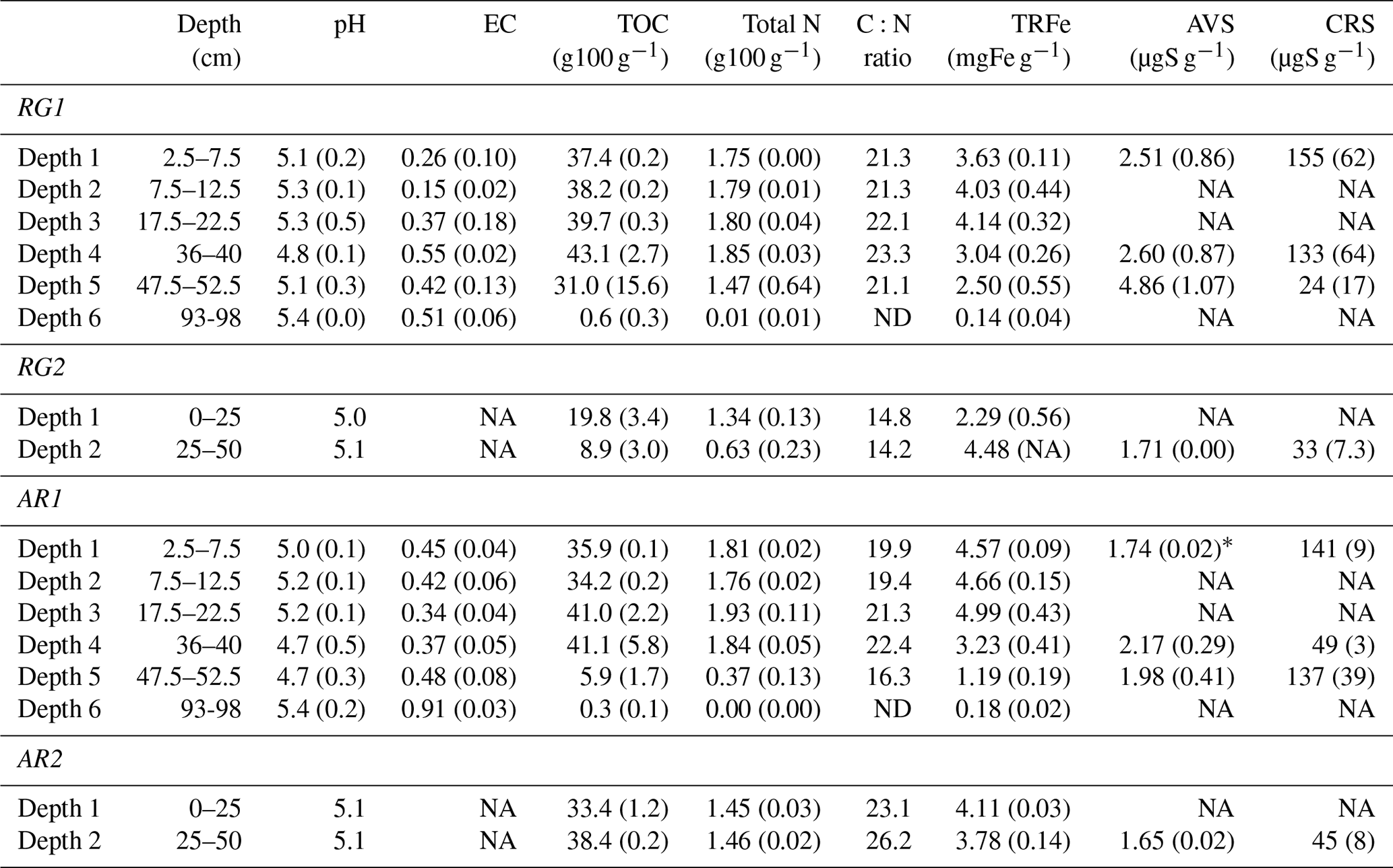
ND – not determined due to TOC and total N concentrations being at the limit of detection. NA – not analysed. * Taghizadeh-Toosi et al. (2019) presented slightly different AVS and CRS results for AR1, representing all the six profiles collected at this site.
The organic matter composition of soil profiles at the four sites varied. Total organic C concentrations at AR1 and RG1 were 34 %–43 % in the upper 0–40 cm but then dropped to only 0.3 %–0.6 % at the ca. 1 m depth in the sand. The peat was amorphous and well-decomposed at the 0–20 cm depth, while the underlying peat contained intact plant debris. At RG2, the process of peat degradation was evident even at the 0–50 cm depth, where total organic carbon (TOC) concentrations only just met the requirements for being defined as an organic soil; the organic C content was below 20 and 10 % at the 0–25 and 25–50 cm depth, respectively. AR2 was characterised by a uniform peat layer (33 %–38 % organic C) at the 0–50 cm depth. Across all sites, the C:N ratios ranged between 14 and 26 in the organic soil layers.
Two iron sulfide fractions, as well as total reactive iron, were quantified. Acid-volatile sulfide ranged from 1.7 to 4.9 µg S g−1 soil across the four sites and showed no clear relationship with soil depth. This was also the case for CRS, which ranged from 24 to 155 µg S g−1 dry weight soil. Total reactive Fe (TRFe) concentrations in soil profiles from AR1 and RG1 ranged from 1.19 to 4.99 mg g−1 of dry weight soil at the 0–50 cm depth, and hence concentrations of reactive Fe were up to 1500 times higher than concentrations of Fe in AVS (assuming this was FeS) and 25–120 times higher than Fe in CRS (assuming this was FeS2). At AR1 and RG1, TRFe declined below the 20 cm depth and was close to zero in the sand below the peat layer (Table 1). The highest concentrations of TRFe at RG1 (Fig. 2b) and AR1 (Fig. 2d) occurred at the 20 cm depth on 23 April (DOY 113). At AR1, a sink for TRFe at the 40–60 cm depth was indicated, and, disregarding Depth 6 (93–98 cm), the concentration of TRFe at Depth 5 (47.5–52.5 cm) was significantly lower than concentrations at more shallow depths (p<0.05). Differences in TRFe concentration were observed at RG1, and any differences in the distribution of TRFe between seasons were probably also minor (not tested). There was a strong correlation between TRFe and TOC across all sites (r=0.88, n=16).
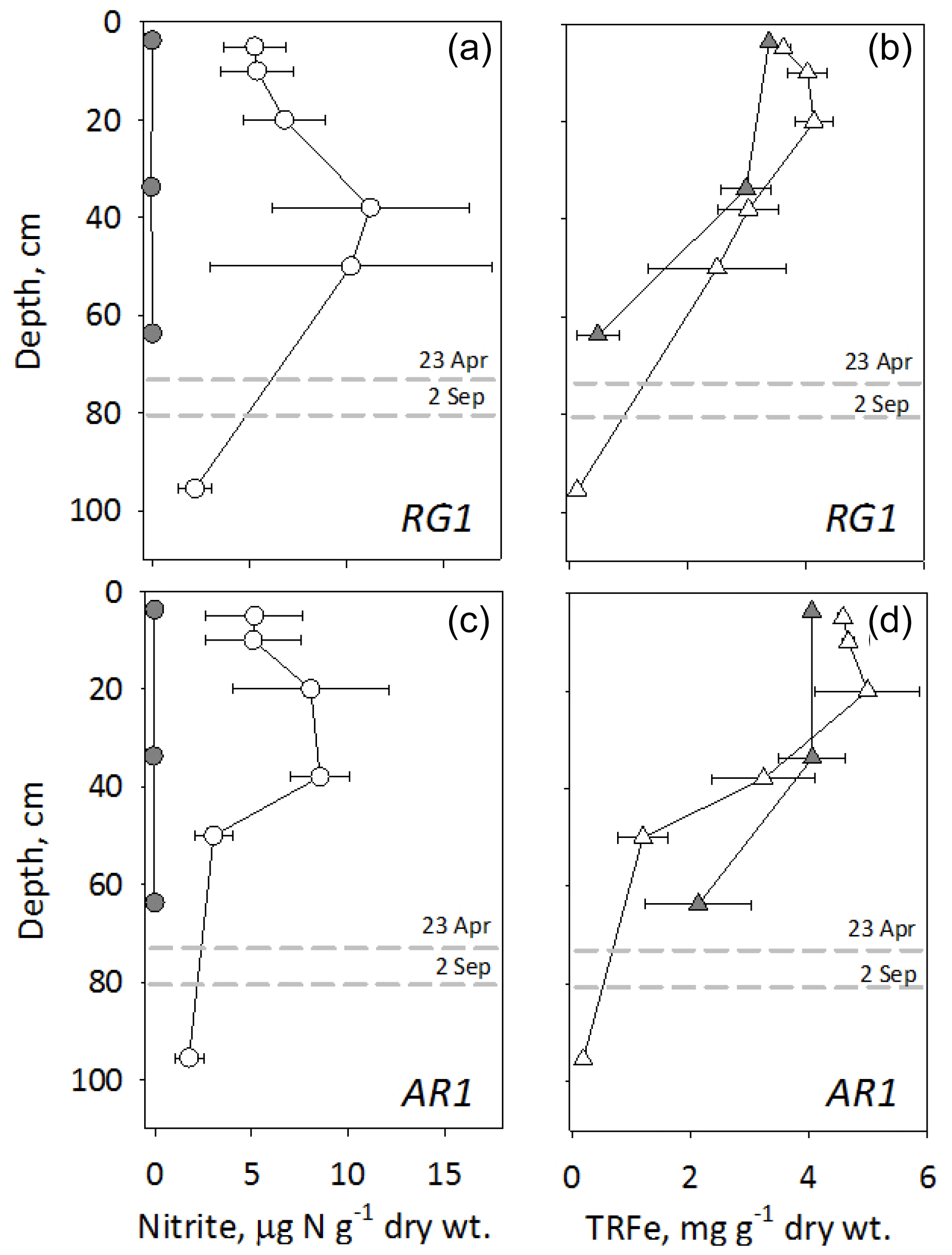
Figure 2Nitrite-N (a, c) and total reactive iron, TRFe (b, d) in undisturbed soil cores were collected at RG1 and AR1 on 23 April (DOY 113; white symbols) and 2 September (DOY 245; grey symbols). Results shown are mean and standard error (n=2). At RG1, fertilisation had taken place 1 week earlier, but a two-sample t test did not find evidence for any effect on availability (p=0.19). The dotted lines indicate WT level on the two sampling dates.
The total reduction capacity was determined by a wet oxidation procedure using Ce(SO4)2. At both AR1 and RG1, the total reductive capacity of the peat at the 27–30 cm depth was outside the range of the analytical method at > 11 500 mequiv kg−1. The reduction capacity dropped to around 1000 mequiv kg−1 at the 60 to 65 cm depth with a declining organic matter content and to 50–100 mequiv kg−1 in the sandy layer at the 93–98 cm depth.
3.3 Soil mineral N dynamics
Soil concentrations of and at the 0–25 and 25–50 cm depth were determined in connection with field campaigns (Tables S1–S4). Since subsamples were pooled for analysis, only a qualitative description of the effects of treatments and temporal dynamics is possible. The residence time for mineral N in the soil solution appeared to be longer at AR compared to RG sites. At AR sites, there was an accumulation of mineral N (Tables S2, S4) at both depth intervals during May that also occurred before N fertilisation. Mineral N concentrations were apparently greater at AR1 compared to AR2, and at AR2, only accumulated. Following fertilisation, -N and -N concentrations were 100–200 µg g−1 of dry weight soil at all sites except RG2 (Table S3 in the Supplement), where acidified cattle slurry was applied. Nitrate accumulated at all sites in the weeks after fertilisation, and also there was evidence for some transport to the 25–50 cm depth.
Nitrite-N concentrations were determined in soil profiles from the cores sampled at RG1 and AR1 on 23 April (DOY 113) and 2 September (DOY 245) 2015. At site RG1, fertilisation had taken place 1 week earlier, but a two-sample t test did not find evidence for an effect on availability (p=0.19), and therefore the results from both AR1 and RG1 subplots are presented together. In April, the average concentration of -N at both sites was highest (ca. 10 µg g−1 of dry weight soil) at around the 40 cm depth and declined towards the surface and deeper layers (Fig. 2a, c). However, due to heterogeneity of soil profiles, the differences between depths were not significant (p=0.22 for RG1 and p=0.06 for AR1). A decline in -N concentration was indicated at the 50 cm depth at AR1, where a depletion of TRFe was indicated. However, there was also less organic matter (cf. TOC in Table 1), which may account for this difference. In September, -N concentrations were < 1 µg g−1 of dry weight soil at both sites, while the concentrations of TRFe were comparable to those in April.
3.4 Groundwater table dynamics
Across the four sites, WT changes ranged from 60 to 100 cm. During spring, the WT depth at RG1 and AR1 varied between 17 and 81 cm, with a steady decline until the end of April, and by DOY 119 the WT depth was significantly (all p values < 0.05) below that of all previous samplings except DOY 112 (Figs. 3 and 4). Then a period with frequent rainfall followed, where WT fluctuated (no significant changes) at around the 60–80 cm depth. During the first half of September (DOY 246 to 259), rainfall caused the WT to rise from the 80 to 40 cm depth (p<0.05; Figs. 5 and 6). On two occasions (DOY 248 and 260) the WT depth rose to 20 cm and only gradually declined during the following days (data not shown). From mid-September (DOY 258) a period with a gradual WT decline followed until early November (DOY 308), whereby the WT showed an increasing trend from the 90 to 45 cm depth during a week with intense rainfall. At RG2 (Fig. 3) the WT initially declined (p<0.05) and then remained mostly at the 50–60 cm depth during spring, with a temporary rise to the 30 cm depth on 3 June (DOY 139; p<0.05). In the autumn, sampling campaigns were resumed on DOY 245. By this time the WT was close to the surface following intense rainfall but then declined (p<0.05) to 80–100 cm in the sandy subsoil (Fig. 5). The WT depth at AR2 declined initially (p<0.01) and then fluctuated between 45 and 60 cm during spring except for a transient increase (p=0.05) to 35 cm in early June (Fig. 4). During autumn the WT rose (p=0.05) to the soil surface in September (DOY 260) and then gradually withdrew (p = 0.05) until early November (DOY 307), when rainfall caused a ca. 40 cm increase (Fig. 6), as also observed at RG1 and AR1.
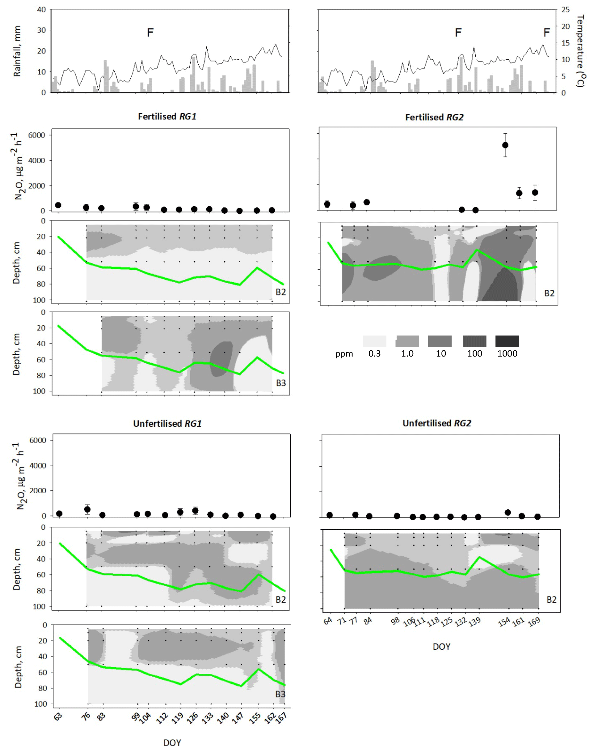
Figure 3The top panel shows rainfall, air temperature and management (F – fertilisation) at RG1 (left panels) and RG2 (right panels) during spring, 3 March (DOY 63) to 16 June (DOY 169). The middle section shows N2O fluxes (black circles; mean ± standard error, n=3) and contour plots of soil N2O concentrations in fertilised subplots, and the lower section shows the corresponding results for unfertilised subplots. A logarithmic grey scale was used in order to show trends within both RG and AR treatments and between depths. Soil gas sampling positions are indicated in the contour plots; numbers shown are N2O concentrations (µL L−1). Green lines show the WT depth (which varied slightly between blocks). B2 and B3 refer to block number of diffusion probe positions.
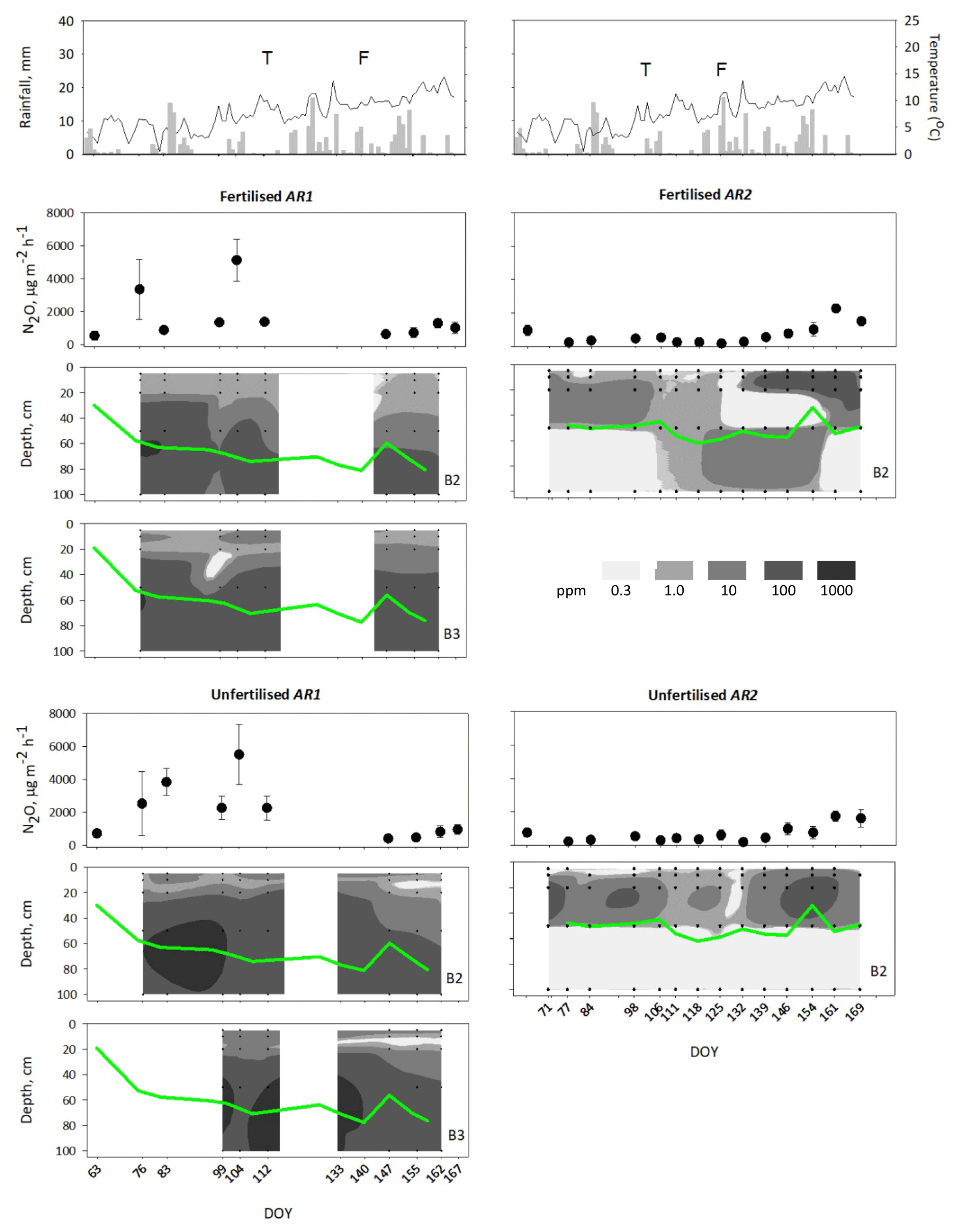
Figure 4The top panel shows rainfall, air temperature and management (T – tillage; F – fertilisation) at AR1 (left panels) and AR2 (right panels) during spring, 3 March (DOY 63) to 16 June (DOY 169). The middle section shows N2O fluxes (black circles; mean ± standard error, n=3) and contour plots of soil N2O concentrations in fertilised subplots, and the lower section shows the corresponding results for unfertilised subplots. A logarithmic grey scale was used in order to show trends within both RG and AR treatments and between depths. Soil gas sampling positions are indicated in the contour plots; numbers shown are N2O concentrations (µL L−1). Gaps are indicated where soil gas sampling probes were installed late or removed due to field operations. Green lines show the WT depth (which varied slightly between blocks). B2 and B3 refer to block number of diffusion probe positions.
3.5 Soil N2O concentration profiles
Equivalent gas-phase concentrations of N2O in passive diffusion samplers were determined concurrently with gas sampling, and results are presented as contour plots (Figs. 3–6; data in Table S5). Concentrations in many cases varied by several orders of magnitude between sites and sampling days, and between depths within individual profiles, and therefore a logarithmic grey scale is used to show gradients. The gaps in Figs. 3–6 indicate periods where diffusion probes could not be installed or were temporarily removed due to field operations.
The concentrations of N2O at grassland sites varied between 0 and 25 µL L−1, with an exception mentioned below. Under the rotational grass at RG1, soil N2O concentrations during spring were mostly between 0.1 and 3 µL L−1 (Fig. 3). A higher concentration (15 µL L−1) was observed at the 40–80 cm depth in the fertilised subplot around DOY 139 but only at the lower position (Block 3) of the field plot. At RG2, the concentrations of N2O in the soil during spring were generally similar to those of RG1, although there were more values in the 1–10 µL L−1 concentration range in the unfertilised plot (Fig. 3; Table S5). However, on 3 June (DOY 154), a much higher N2O concentration was observed in the fertilised part of the plot with a maximum of 560 µL L−1 at the 100 cm depth (i.e. well below the WT). Soil N2O concentrations in the unfertilised plot were also elevated around this time but only to a maximum of 15 µL L−1 and mainly near the soil surface.
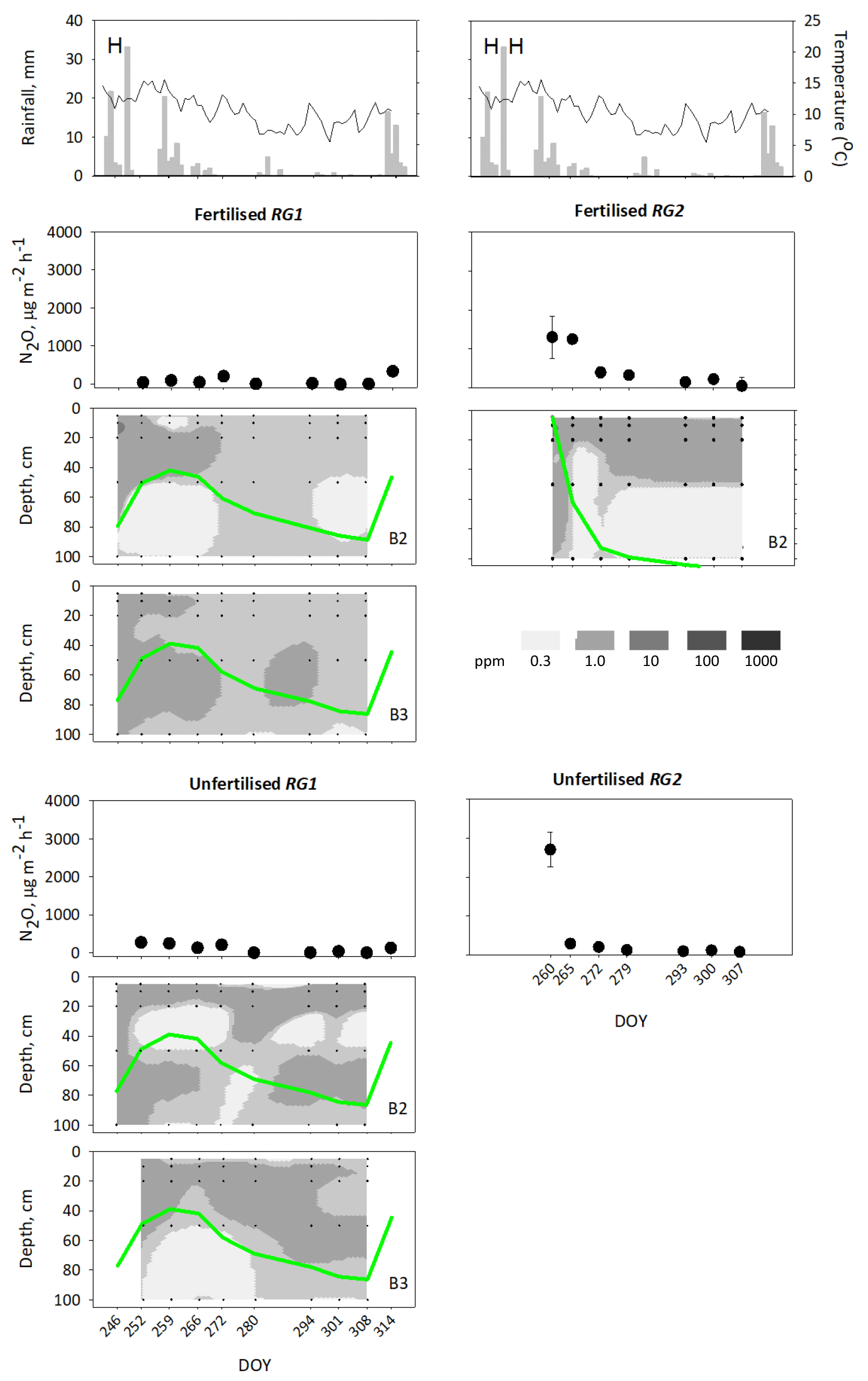
Figure 5The top panel shows rainfall, air temperature and management (H – harvest) at RG1 (left panels) and RG2 (right panels) during autumn, 3 September (DOY 245) to 10 November (DOY 314). The middle section shows N2O fluxes (black circles; mean ± standard error, n=3) and contour plots of soil N2O concentrations in fertilised subplots, and the lower section shows the corresponding results for unfertilised subplots. A logarithmic grey scale was used in order to show trends within both RG and AR treatments and between depths. Soil gas sampling positions are indicated in the contour plots; numbers shown are N2O concentrations (µL L−1). The probes were absent in the unfertilised subplot after harvest. Green lines show the WT depth (which varied slightly between blocks). B2 and B3 refer to block number of diffusion probe positions.
The arable AR1 site, with sampling positions located in a different field, but only 10–20 m from those of RG1, had apparently very different soil N2O concentration dynamics during spring (Fig. 4). There was a consistent accumulation of N2O at the 50 and 100 cm depth, where seasonal concentrations averaged at 340 and 424 µL L−1, respectively. In contrast, at the 5, 10 and 20 cm depth, the average N2O concentrations were 10–30 µL L−1, and there was no clear response to fertilisation on DOY 141 in terms of soil N2O accumulation. The soil N2O concentrations suggested that there was considerable within-site heterogeneity in soil conditions, as the highest concentrations were often observed in the unfertilised subplot. Maximum concentrations of N2O of nearly 1500 µL L−1 were recorded at the 50 cm depth on DOY 99 and a similar concentration at the 100 cm depth on DOY 112, both in the unfertilised subplot. At AR2, the highest soil N2O concentrations during early spring were consistently observed at the 20 cm depth but seemed to gradually decline to reach the background level of 0.3 µL L−1 in mid-May (around DOY 130). In the unfertilised subplot, the N2O concentration reached 272 µL L−1 at the 20 cm depth following rainfall and with WT at the 35 cm depth. With fertilisation, soil N2O concentrations at the 10 cm depth reached nearly 400 µL L−1 in mid-June. The observed accumulation of N2O near the soil surface was accompanied by increasing N2O emissions during this period (Fig. 4).
During autumn, N2O concentrations in the soil profile at the RG1 and RG2 sites varied between 0 and 12 µL L−1, with a tendency for higher concentrations at the 10–20 cm depth (Fig. 5). At RG1, where both fertilised and unfertilised subplots could be sampled, this was apparently independent of fertilisation.
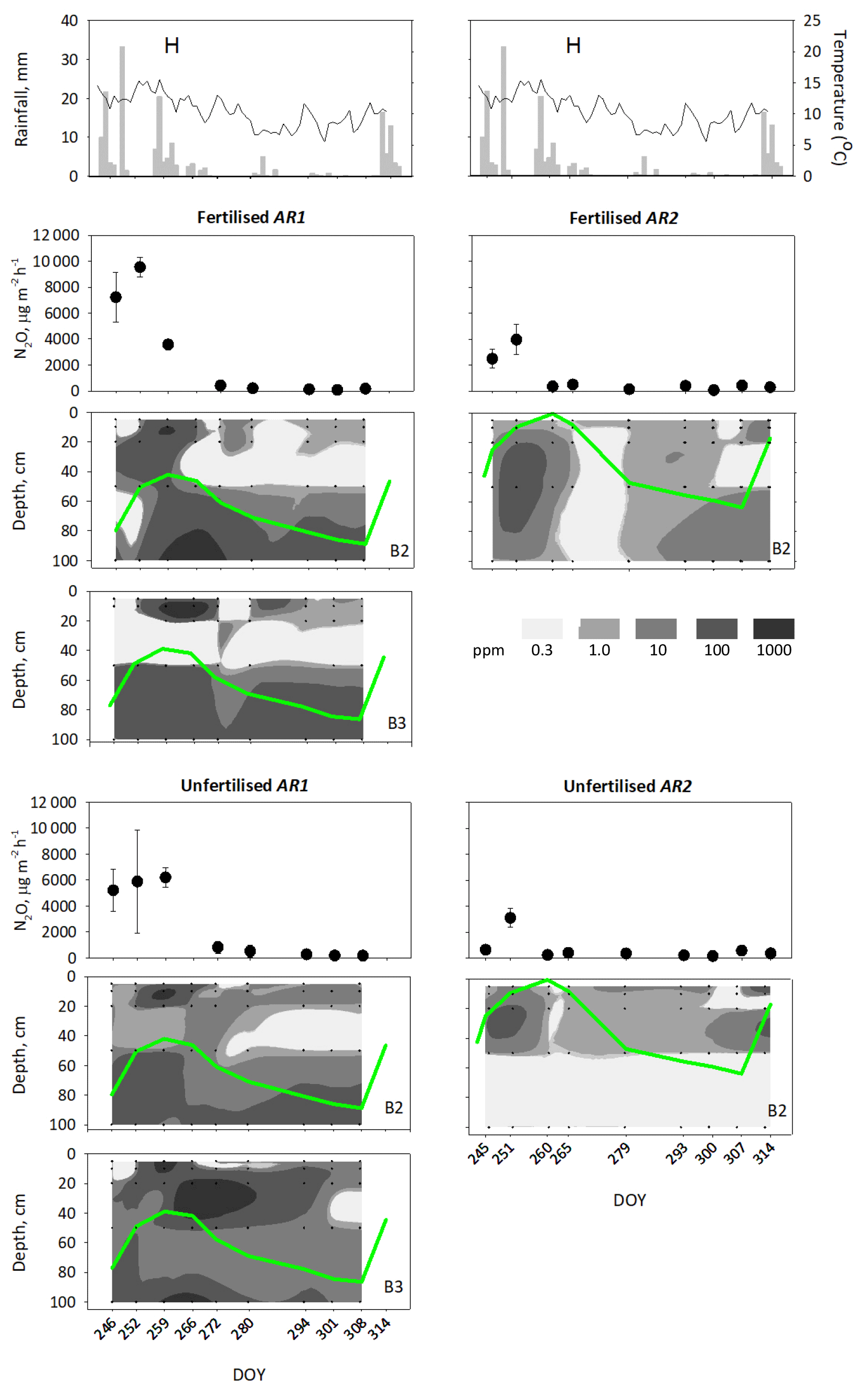
Figure 6The top panel shows rainfall, air temperature and management (H – harvest) at AR1 (left panels) and AR2 (right panels) during autumn, 3 September (DOY 245) to 10 November (DOY 314). The middle section shows N2O fluxes (black circles; mean ± standard error, n=3) and contour plots of soil N2O concentrations in fertilised subplots, and the lower section shows the corresponding results for unfertilised subplots. A logarithmic grey scale was used in order to show trends within both RG and AR treatments and between depths. Soil gas sampling positions are indicated in the contour plots; numbers shown are N2O concentrations (µL L−1). Green lines show the WT depth (which varied slightly between blocks). B2 and B3 refer to block number of diffusion probe positions.
September was characterised by heavy rainfall (114 mm in total), and at AR1 a substantial rise in the WT from the 80 to 40 cm depth was observed (Fig. 6). Soil N2O concentrations showed a pattern with maxima at the 10 and 100 cm depth through to DOY 266 (end of September), and after this time, soil N2O accumulation rapidly declined concurrently with WT drawdown. Nitrous oxide concentrations equivalent to several hundred microlitres per litre were measured even at the 5 cm depth during this period, and the overall highest concentration recorded was 2270 µL L−1 at the 10 cm depth on DOY 266. During late autumn, the N2O concentration at the 0–50 cm depth varied between 0 and 20 µL L−1, whereas at the 100 cm depth it remained high at 100–850 µL L−1. At AR2, the groundwater level was higher than at AR1 and came close to the soil surface by mid-September (DOY 260). Soil N2O accumulated in both fertilised and unfertilised subplots following saturation of the soil; again the highest concentrations apparently occurred at the 20 cm depth. A secondary increase was observed near the soil surface at the last sampling on DOY 314 in November, in response to a period with rainfall and a rapid WT rise.
3.6 Nitrous oxide emissions
The weekly sampling campaigns during spring and autumn showed that with a few exceptions, N2O emissions, expressed as average daily rates, were significantly higher at arable compared to grassland sites (Table 2). One exception was treatment RG2-F in spring, where a peak in N2O emissions was indicated (p=0.06) on DOY 154, and the flux was still elevated at the next two samplings (Fig. 3). This high flux coincided with the accumulation of N2O in the soil profile described above, and it was the only time that an effect of fertilisation was observed. The grass in the fertilised subplot showed a clear visual response to fertilisation, which indicated that fertiliser N was effectively taken up by the sward.
Table 2Daily emissions of N2O during the monitoring periods in spring and autumn were analysed with a generalised linear mixed model (see text). Estimation for each season was performed using the trapezoidal approximation of the integral of the emission curve. Numbers in brackets indicate 95 % confidence intervals, and significant differences between all eight treatments within each season (at 5 % significance level, with correction for multiple testing by the single-step method) are indicated by letters.
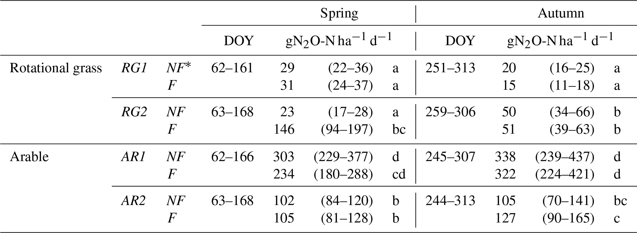
* F – fertilised. NF – not fertilised.
At AR1 the N2O fluxes during early spring reached 2000–6000 µgN2O m−2 h−1 and were higher than in late spring (Fig. 4). Since there was no effect of N fertilisation (see Table 2), the higher emissions were probably derived from soil N pools and caused by factors other than fertilisation. The potato field at AR2 showed a different pattern, with N2O fluxes remaining low during early spring and for several weeks after fertilisation. Independent of fertilisation, an increasing trend (not significant) was observed in June following a rise in WT, which was at the 35 cm depth on DOY 154.
In the autumn, N2O fluxes from RG1 were consistently low (Fig. 5). The first sampling at RG2 was on DOY 259 in mid-September, where a high flux of 3000 µgN2O m−2 h−1 was seen, which dropped to near zero within 1–2 weeks. Nitrous oxide emissions at AR1 were high during September at 4000–10 000 µgN2O m−2 h−1 across the two N fertilisation treatments and subsequently declined (p<0.05) to near zero (Fig. 6). High fluxes were observed on the first day of this monitoring period, DOY 246, at a time where the WT depth was still at the 40 to 80 cm depth. Instead the high N2O fluxes may have been triggered by saturation of the topsoil after 10 and 22 mm rainfall the previous 2 d. Additional rainfall during the following days was then accompanied by a rise in WT. The subsequent decline in N2O emissions at AR sites coincided with WT drawdown and drainage of the topsoil.
Cumulative N2O emissions were calculated for the 99–105 d monitoring period in spring as well as the 47–69 d period in the autumn. Daily rates were surprisingly consistent in the two periods (Table 2), and therefore the following refers to cumulative emissions across both periods. At RG1, the total emission was 4 kg N2O-N ha−1 independent of fertilisation, whereas at RG2 the fertilised and unfertilised subplots were different at 18 and 5 kg N2O-N ha−1, respectively. At AR sites with potatoes, there was no effect of N fertilisation, and the cumulative N2O emissions were 18–20 kg N2O-N ha−1 at AR2 but much higher at 44–52 kg N2O-N ha−1 at AR1.
3.7 Interrelationships between driving variables of N2O production
Graphical models were used to study the dependence structure among selected soil variables and N2O fluxes. Interestingly, at both RG sites, and in both seasons, N2O flux consistently depended on N2OWT, i.e. soil N2O concentration in the capillary fringe (Fig. 7a and b and Fig. 8a and b). This was also the case for both AR sites in spring (Fig. 7c and d). Where N2OWT separated N2O flux from other variables in the graph, this indicates, according to the separation principle (Sect. 2.5), that information about N2OWT rendered all the other variables uninformative with respect to N2O flux. For example, in the analysis of AR1 in spring (Fig. 7b), the variables N2O flux and Temp5 were not directly connected, and therefore any correlation between Temp5 and N2O flux could be completely explained by other variables.
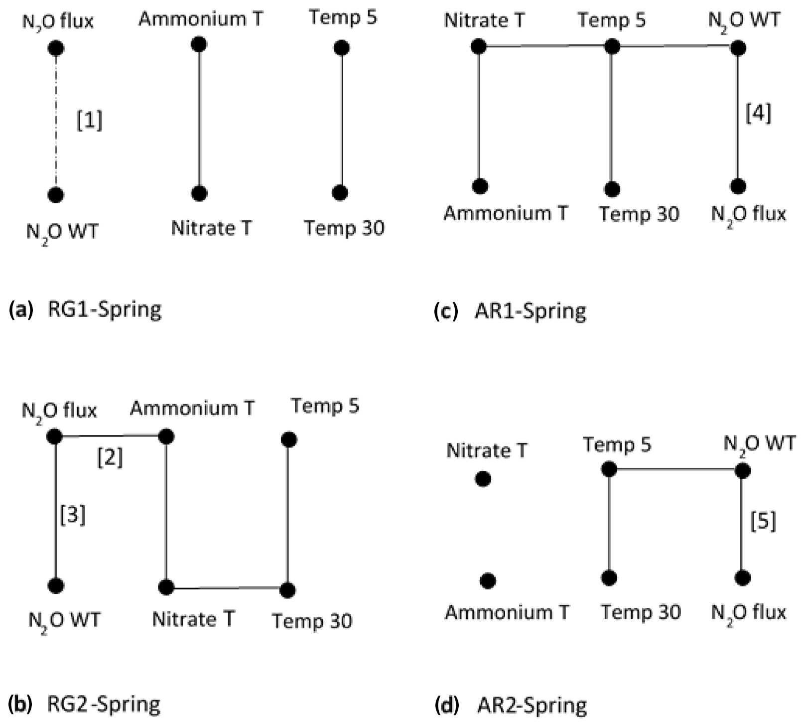
Figure 7Results of a graphical model for each site–crop combination in spring: (a) RG1-Spring, (b) RG2-Spring, (c) AR1-Spring, and (d) AR2-Spring. The edges (lines) connecting vertices (points) indicate significant conditional correlation between the variables given the other variables. The statistical results for direct effects on N2O flux are as follows: [1] 0.14 (0.02–0.23, p=0.067), [2] 0.13 (0.06–0.21, p=0.008), [3] 0.18 (0.09–0.26, p=0.001), [4] 0.15 (0.04–0.23, p=0.032) and [5] 0.37 (0.12–0.49, p=0.002). Key to variables: Ammonium T – -N at 0–25 cm depth, Nitrate T – -N at 0–25 cm depth, N2O WT – equivalent soil gas-phase concentration closest to but above the water table depth, Temp 5 – soil temperature at 5 cm depth – and Temp 30 – soil temperature at 30 cm depth.
The graphical model results were different for AR sites in the autumn (Fig. 8c and d), where instead soil temperature at the 30 cm depth and (AR1 only) -N concentration in the topsoil showed significant correlation with N2O flux (p<0.05). All other variables were unrelated to N2O flux or could be accounted for by other variables.
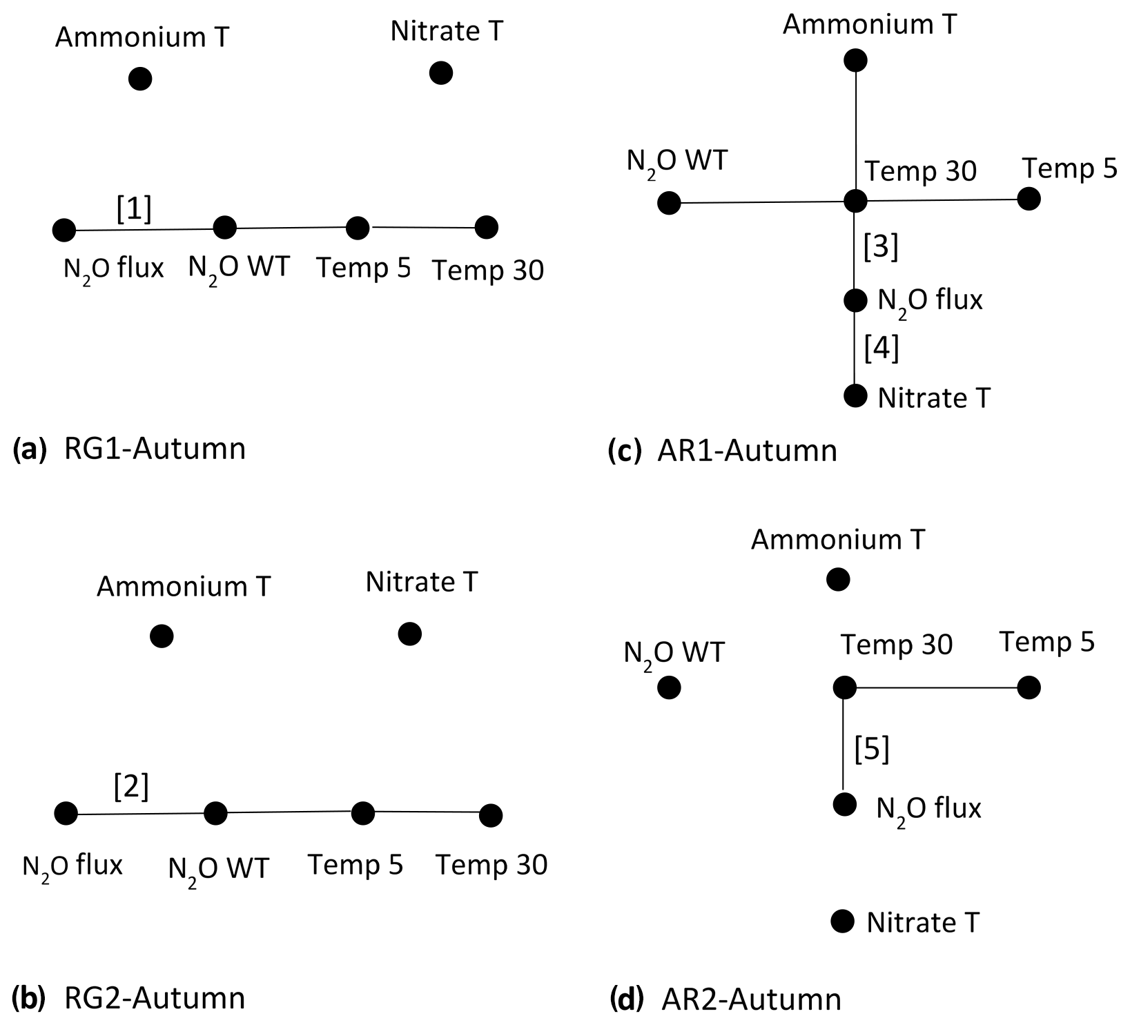
Figure 8Results of a graphical model for each site–crop combination in the autumn. (a) RG1-Autumn, (b) RG2-Autumn, (c) AR1-Autumn and (d) AR2-Autumn. The edges (lines) connecting vertices (points) indicate significant conditional correlation between the variables given the other variables. Statistical results for effects on N2O flux are as follows: [1] 0.27 (0.19–0.38, p=0.002), [2] 0.16 (0.007–0.28, p=0.049), [3] 0.19 (0.09–0.28, p=0.021), [4] 0.15 (0.06–0.21, p=0.032) and [5] 0.29 (0.17–0.35, p=0.005). Key to variables: Ammonium T – -N at 0–25 cm depth, Nitrate T – -N at 0–25 cm depth, N2O WT – equivalent soil gas-phase concentration closest to but above the water table depth, Temp 5 – soil temperature at 5 cm depth – and Temp 30 – soil temperature at 30 cm depth.
This study investigated seasonal dynamics of N2O emissions and soil conditions in an area, which has been designated as a hotspot for N2O emissions (Leppelt et al., 2014). Spring and autumn monitoring periods together covered between 152 and 174 d, and cumulative N2O emissions during these periods were in total 4–5 kg N2O-N ha−1 for rotational grass if disregarding the 2-week period after slurry application at RG2-F and 20–50 kg N2O-N ha−1 for arable sites with a potato crop. These numbers, representing < 6-month periods, thus confirmed previous results (Petersen et al., 2012) that annual N2O emissions from organic soil in this area are comparable to (RG), or clearly above (AR), the IPCC emission factors for drained organic soil of 8 and 13 kg N2O-N ha−1 yr−1 for nutrient-rich grassland and cropland, respectively (IPCC, 2014). The area has been characterised as potentially acid sulfate soil (Madsen and Jensen, 1988), and a previous study showed groundwater sulfate concentrations in excess of 100 mg L−1 (Petersen et al., 2012). We therefore hypothesised that reduction coupled with FeS2 oxidation could be a pathway of N2O formation in this acid organic soil.
Pyrite, measured as CRS, was quantified at selected depths (Table 1). Soil bulk density of the peat varied between 0.15 and 0.3 g cm−3 (data not shown), and the total amount of CRS at the 0 to 50 cm depth could therefore be estimated to 200–350 mmolFeS2 m−2. The N2O emissions observed during spring and autumn monitoring periods constituted up to 145 mmol N m−2 in total (AR1), and it is thus theoretically possible that the process described by Eq. (2) contributed to emissions of N2O. However, the FeS2 concentration (0.4–2.4 mmol kg−1) represented a minor part of the total reduction capacity (> 11 500 mequiv kg−1 at the 27–30 cm depth). Also, average concentrations of total reactive Fe were 25–120 times higher than those of FeS2 (though less in terms of reduction equivalents). It is therefore likely that reducing agents other than FeS2 were important, a conclusion that was later supported by a laboratory study in which peat amended with FeS2 did not show enhanced N2O production (Taghizadeh-Toosi et al., 2019). Other possible drivers of N2O emissions were therefore considered.
4.1 Environmental drivers of N2O emissions
A limited number of potential drivers (rainfall, temperature, soil mineral N and soil concentrations of N2O) were monitored to help explain N2O emission dynamics. Soil N2O concentration profiles showed complex patterns where, for example, the highest concentrations were sometimes observed above and sometimes below the WT depth at both RG (Fig. 3) and AR sites (Fig. 4). Fertilisation in spring was associated with higher concentrations of N2O below the WT depth at RG2 and AR2, which indicated downward transport of fertiliser N, but this was not reflected in elevated N2O emissions. The reason may be that in wet soil the time required to reach a steady state between N2O production and emissions from the soil surface can be significant and increases with distance (Jury et al., 1982). In accordance with this, Clough et al. (1999) observed a delay of 11 d before 15N-enriched N2O produced at the 80 cm depth was released from the soil surface at a corresponding rate. Since the presence of air-filled porosity is critical for the exchange of gases between soil and the atmosphere (Jury et al., 1982), the soil N2O concentration closest to but above the WT depth (N2OWT) was taken to represent “subsoil” processes stimulating N2O emissions.
The regulation of N2O emissions was investigated using a statistical method represented by graphical models. Among the factors considered, the graphical models for individual site–crop combinations consistently identified N2O concentration in the capillary fringe as the strongest predictor of N2O emissions from both grassland and arable sites in spring (Fig. 7a–d) and from grassland sites in the autumn (Fig. 8a and b). The implication is that N transformations deeper in the soil, and not in the topsoil, were the main source of N2O escaping to the atmosphere in these cases. In accordance with this, there was no apparent effect of N fertilisation on emissions of N2O, with emissions at RG2 after the application of acidified cattle slurry being a notable exception. Other studies also found a limited response to fertilisation (Maljanen et al., 2003; Regina et al., 2004), although Regina et al. (2004) later observed a peak in N2O emissions after rainfall. Goldberg et al. (2010) reported that N2O emissions from minerotrophic fen were produced at the 30–50 cm depth, in accordance with the observations presented here, where the highest concentrations of N2O were mostly observed at the 20 or 50 cm depth (Table S5).
Peat decomposing in the capillary fringe during WT drawdown could have been the source of N for N2O production. It is well established that N2O emissions from organic soil may be enhanced by drainage (Martikainen et al., 1993; Taft et al., 2017), and the response will appear within days, as shown by Aerts and Ludwig (1997) in an incubation study with an oscillating WT. A stimulation of N2O emissions by WT drawdown was also observed by Goldberg et al. (2010) when simulating drought under field conditions, although a pulse of N2O also occurred after rewetting in that study. In accordance with this effect of rewetting, rain events during late spring and early autumn often enhanced N2O emissions. This was not necessarily a result of WT changes. Despite 32 mm rainfall on DOY 244 and 245, the WT depth at AR1 was still at 40 to 80 cm on DOY 246 (Fig. 6), but N2O emissions were high. Well-degraded peat will release as little as 10 % of its water to drainage (Rezanezhad et al., 2016), and it is therefore likely that rainwater was absorbed by peat above the WT and created conditions suitable for denitrification close to the soil surface, which explains the significant correlation between N2O emissions and (Fig. 8c).
The increase in N2O emissions during WT cycles reported by Aerts and Ludwig (1997) was observed only with eutrophic peat, whereas mesotrophic peat showed no effect of WT dynamics on N2O emissions, which were consistently low. A similar interaction between nutrient status and WT depth was observed in field studies comparing N2O emissions from minerotrophic and ombrotrophic boreal peatlands (Martikainen et al., 1993; Regina et al., 1996). In the present study, soil -N and -N concentrations at RG1 increased to 133 and 120 µg g−1 of dry weight soil upon fertilisation, respectively, but largely returned to the background level of around 5 and 10 µg g−1 dry weight soil, respectively, within a week (Table S1). In contrast, at AR1, there was substantial accumulation of -N and -N even before fertilisation on DOY 141, and soil mineral N remained high for several weeks (Table S2), which may have stimulated N2O emissions in the arable soil. Grasslands on organic soil generally show lower emissions of N2O compared to arable organic soil (Eickenscheidt et al., 2015), presumably because plants compete successfully with microorganisms for available N. Schothorst (1977) estimated peat decomposition indirectly from the N content in the herbage yield of grassland and concluded that the soil supplied 96 kg N ha−1 when the drainage depth was 25 cm but 160 and 224 kg N ha−1 with the drainage depth at 70 and 80 cm, respectively. Hence, plant uptake of N mineralised from soil organic matter above the WT likely contributed to the much lower N2O emissions from rotational grass in this study.
At RG sites, soil N2O concentrations during spring were generally low and thus did not show evidence for microbial N transformations, which supports the conclusion above that plant uptake was a main sink for the N released during peat decomposition. One exception was the accumulation of N2O at the 50–100 cm depth observed at RG2 in late May (Fig. 3), which could have been caused by the leaching of mineral N from the acidified cattle slurry following extensive rain. In contrast, at AR sites, N2O accumulated in the soil throughout spring irrespective of fertilisation; at AR1 the highest concentrations occurred at the 50 and 100 cm depth, while at AR2, with a higher groundwater table, the highest concentrations were at the 20 cm depth. It showed that peat decomposition was a source of mineral N and a likely source of N2O above and possibly also below the saturated zone (see next section).
In the autumn, the graphical models identified in the topsoil (AR1 only) and soil temperature at the 30 cm depth as predictors of N2O emissions at arable sites (Fig. 7). The accumulation of was much greater at AR1 compared to AR2, which was possibly because AR1 had better drainage of the topsoil (e.g. WT at 80 vs. 40 cm depth on DOY 246; Fig. 6). It is not clear if the source of N was decomposing potato top residues, accelerated peat decomposition or both. Rainfall most likely triggered denitrification by increasing soil-water-filled pore space and raising WT depth, thereby impeding the O2 supply to much of the soil profile (Barton et al., 2008). This interpretation is supported by increasing N2O concentrations below as well as above the WT depth depending on the site and block, and in fertilised as well as unfertilised subplots (Fig. 6). In an annual study, conducted in other parts of the Store Vildmose, Kandel et al. (2018) also measured high emissions of N2O from a potato crop, i.e. around 2000 µgN2O m−2 h−1 in October 2014 and 6000 µgN2O m−2 h−1 in June 2015, which coincided with accumulation and rainfall. Precipitation was also high during September 2015, and this was accompanied by accumulation of N2O in the topsoil at all sites. However, N2O concentrations reached only around 10 µL L−1 at RG sites, as opposed to several hundred microlitres per litre at AR sites, confirming that soil mineral N availability was a limiting factor for N2O emissions.
4.2 Pathways of N2O emissions
Bacterial nitrification, denitrification and nitrifier denitrification are all potentially significant pathways of N2O formation (Braker and Conrad, 2011). The correlation with in the topsoil at AR1 in the autumn (Fig. 8c) suggested that here denitrification activity controlled N2O emissions, but mostly soil mineral N concentrations were low, and ammonia oxidation activity may have limited N2O emissions either directly, or indirectly, via production of or . Ammonia-oxidising bacteria (AOB) are scarce in acid peat despite the presence of nitrite-oxidising bacteria (NOB; Regina et al., 1996), and some studies indicate that ammonia-oxidising archaea (AOA) predominate in both abundance and activity (Herrmann et al., 2012; Stopnišek et al., 2010). Stieglmeier et al. (2014) isolated AOA from soil that emitted N2O at a rate corresponding to 0.09 % of the produced independent of O2 availability, but it is not known if this organism is present in acid organic soil, and at this time an indirect control of denitrification activity seems more plausible.
Stopnišek et al. (2010) found that AOA activity was not stimulated by an external source of and concluded that the activity was associated with N released from decomposing soil organic matter. Well-decomposed peat is dominated by dead-end pores associated with plant cell remains, which are characterised by a slow exchange of solutes with active pore volumes (Hoag and Price, 1997), and hence ammonia oxidation in confined spaces could be important in organic soil. The anaerobic conditions of saturated peat may have limited N mineralisation and hence ammonia oxidation activity during early spring, a constraint which was removed as the WT declined and O2 entered deeper soil layers. Estop-Aragonés et al. (2012) found that oxic–anoxic interfaces in peat soil were located above the WT depth, and hence the capillary fringe may have been still partly anoxic, which can explain the correlation between N2OWT and N2O emissions in graphical models. In late April (DOY 113), had accumulated at the 20–50 cm depth at both RG1 and AR1 sites (Fig. 2), suggesting that there was an imbalance between ammonia oxidation and nitrite oxidation activity. Oxygen affinity differs between nitrifiers, with AOA > AOB > NOB (Yin et al., 2018), and hence O2 limitation could have caused the accumulation of . In acid soil, this would result in product inhibition by HNO2 if there were no mechanism to remove ; this would be especially true for AR sites, where mineral N accumulation was 3 to 4 times higher compared to RG sites (Tables S3–S6). Nitrifier denitrification is a mechanism by which ammonia oxidisers can avoid HNO2 accumulation, and this process leads to N2O formation (Braker and Conrad, 2011). Another potential sink for is chemodenitrification, an abiotic reaction in which reacts with Fe2+ to produce N2O (Jones et al., 2015):
where in Eq. (4), Fe(OH)3 is shown as anhydrous FeOOH. A possible depletion of TRFe was indicated at the 50 cm depth at AR1, which coincided with a similar pattern for (Fig. 2). Nitrifier denitrification and chemodenitrification are both sinks for , and therefore both pathways are potential sources of the N2O emissions observed during early spring.
At AR sites there was often considerable accumulation of N2O below the WT, which suggests that there was also an anaerobic pathway of N2O formation. The fact that TRFe concentrations were much higher than those of AVS or CRS (Table 1) makes it relevant to consider alternative reactions involving iron oxides and hydroxides, which have the potential to produce N2O. One such recently described pathway is Feammox, a process whereby ammonia oxidation coupled with ferric iron reduction can produce below pH 6.5 (Yang et al., 2012):
Nitrate can also be produced under these conditions (Yang et al., 2012; Guan et al., 2018):
A shuttle of Fe2+ between Feammox and chemodenitrification (Eqs. 5 and 4) could account for the accumulation of N2O under anoxic conditions in the saturated zone, presumably with the availability of from peat mineralisation as a limiting factor. The confirmation of pathways will require more detailed investigations that should include molecular analyses targeting microbial communities in the soil profile.
In this 1-year study, N2O emissions from arable sites were consistently higher compared to those from rotational grass. There were strong seasonal dynamics in N2O emissions, and we present evidence that different pathways were involved. Concentrations of pyrite were low compared to the total reduction capacity of the peat, and Fe was predominantly in forms other than pyrite. The hypothesis that reduction coupled with FeS2 oxidation was an important source of N2O could therefore not be confirmed. Nitrous oxide emissions during spring were independent of fertilisation, since there was mostly no effect of mineral N in the topsoil. The significant effect of N2O concentration in the capillary fringe indicated that emissions during spring, and for grassland also during the autumn, were associated with soil N mineralisation in this environment, as modified by rainfall patterns and WT dynamics. We propose that chemodenitrification (or nitrifier denitrification) of produced in the capillary fringe is a main source of N2O in acid organic soil during spring, whereas in the autumn heterotrophic denitrification can be a main pathway in arable soil as a result of accumulation. Mitigating N2O emissions from acid organic soil is challenged by this complexity of underlying processes. However, reducing mineral N accumulation by ensuring a vegetation cover outside the main cropping season and stabilising the WT depth by effective drainage are potential mitigation strategies.
Soil characteristics are presented in Table 1, and soil mineral N in Tables S1–S4 is presented in the Supplement. Equivalent soil gas-phase concentrations of N2O used to create contour plots in Figs. 3–6 are available in Table S5. Nitrous oxide fluxes and climate data are available upon request to arezoo.taghizadeh-toosi@agro.au.dk.
The supplement related to this article is available online at: https://doi.org/10.5194/bg-16-4555-2019-supplement.
ATT, LE, TJC and SOP designed the study. ATT, LE, VE and SOP carried out sampling and analyses. ATT, RL and SOP were responsible for data analyses. ATT and SOP prepared the paper, with contributions from all co-authors.
The authors declare that they have no conflict of interest.
We would like to thank the dedicated staff involved in field campaigns, including Bodil Stensgaard, Søren Erik Nissen, Sandhya Karki, Kim Johansen, Karin Dyrberg, Holger Bak and Stig T. Rasmussen. We would also like to acknowledge the support of three farmers hosting the field sites: Poul-Erik Birkbak, Rasmus Christensen and Jørn Christiansen.
This research has been supported by the Danish Research Council for the project “Sources of N2O in arable organic soil as revealed by N2O isotopomers” (grant no. DFF – 4005-00448).
This paper was edited by Ji-Hyung Park and reviewed by two anonymous referees.
Abreu, G. C. G., Edwards, D., and Labouriau, R.: High-dimensional graphical model search with the gRapHD R package, J. Stat. Softw., 37, 1–18, https://doi.org/10.18637/jss.v037.i01., 2010.
Aerts, R. and Ludwig, F.: Water-table changes and nutritional status affect trace gas emissions from laboratory columns of peatland soils, Soil Biol. Biochem., 29, 1691–1698, https://doi.org/10.1016/S0038-0717(97)00074-6, 1997.
Barton, L., Kiese, A., Gatter, D., Butterbach-Bahl, K., Buck, R., Hinz, C., and Murphy, D. V.: Nitrous oxide emissions from a cropped soil in a semi-arid climate, Glob. Change Biol., 14, 177–192, https://doi.org/10.1111/j.1365-2486.2007.01474.x, 2008.
Braker, G. and Conrad, R.: Diversity, structure, and size of N2O-producing microbial communities in soils – what matters for their functioning?, Adv. Appl. Microbiol., 75, 33–70, https://doi.org/10.1016/B978-0-12-387046-9.00002-5, 2011.
Burton, E. D., Sullivan, L. A., Bush, R. T., Johnston, S. G., and Keene, A. F.: A simple and inexpensive chromium-reducible sulfur method for acid-sulfate soils, Appl. Geochem., 23, 2759–2766, https://doi.org/10.1016/j.apgeochem.2008.07.007, 2008.
Carter, M. R. and Gregorich, E. G. (Eds.): Soil sampling and methods of analysis, 2nd Edn., CRC Press, USA, 307–310, 2007.
Cline, J. D.: Spectrophotometric determination of hydrogen sulfide in natural waters, Limnol. Oceanogr., 14, 454–458, https://doi.org/10.4319/lo.1969.14.3.0454, 1969.
Clough, T. J., Jarvis, S. C., Dixon, E. R., Stevens, R. J., Laughlin, R. J., and Hatch D. J.: Carbon induced subsoil denitrification of 15N-labelled nitrate in 1 m deep soil columns, Soil Biol. Biochem., 31, 31–41, https://doi.org/10.1016/S0038-0717(98)00097-2, 1999.
Conen, F. and Smith, K. A.: A re-examination of closed flux chamber methods for the measurement of trace gas emissions from soils to the atmosphere, Eur. J. Soil Sci., 49, 701–707, 1998.
Davidson, A. C. and Hinkley, D. V.: Bootstrap Methods and their Application, 1st Edn., Cambridge University Press, New York, NY, 84 pp., 1997.
Duan, Y. F., Kong, X.-W., Schramm, A., Labouriau, R., Eriksen, J., and Petersen, S. O.: Microbial N transformations and N2O emission after simulated grassland cultivation: effects of the nitrification inhibitor 3,4-Dimethylpyrazole Phosphate (DMPP), Appl. Environ. Microbiol., 83, e02019, https://doi.org/10.1128/AEM.02019-16, 2017.
Eickenscheidt, T., Heinichen, J., and Drösler, M.: The greenhouse gas balance of a drained fen peatland is mainly controlled by land-use rather than soil organic carbon content, Biogeosciences, 12, 5161–5184, https://doi.org/10.5194/bg-12-5161-2015, 2015.
Estop-Aragonés, C., Knorr, K.-H., and Blodau, C.: Controls on in situ oxygen and dissolved inorganic carbon dynamics in peats of a temperate fen, J. Geophys. Res., 117, G02002, https://doi.org/10.1029/2011JG001888, 2012.
Gillham, R. W.: The capillary fringe and its effect on water-table response, J. Hydrol., 67, 307–324, https://doi.org/10.1016/0022-1694(84)90248-8, 1984.
Goldberg, S. D., Knorr, K.-H., Blodau, C., Lischeid, G., and Gebauer, G.: Impact of altering the water table height of an acidic fen on N2O and NO fluxes and soil concentrations, Glob. Change Biol., 16, 220–233, https://doi.org/10.1111/j.1365-2486.2009.02015.x, 2010.
Good, P. I.: Permutation, Parametric and Bootstrap Tests of Hypotheses, Third Edition, Springer, New York, NY, 315 pp., 2005.
Guan, Q. S., Cao, W. Z., Wang, G. J., Wu, F.F., Wang, C., Jiang, C., Tao, Y. R., and Gao, Y.: Nitrogen loss through anaerobic ammonium oxidation coupled with iron reduction in a mangrove wetland, Eur. J. Soil Sci., 69, 732–741, https://doi.org/10.1111/ejss.12552, 2018.
Haughton, D. M. A.: On the choice of a model to fit data from an exponential family, Ann. Statist., 16, 342–335, https://doi.org/10.1214/aos/1176350709, 1988.
Herold, M. B., Baggs, E. M., and Daniell, T. J.: Fungal and bacterial denitrification are differently affected by long-term pH amendment and cultivation of arable soil, Soil Biol. Biochem., 54, 25–35, https://doi.org/10.1016/j.soilbio.2012.04.031, 2012.
Herrmann, M., Hädrich, A., and Küsel, K.: Predominance of thaumarchaeal ammonia oxidizer abundance and transcriptional activity in an acidic fen, Env. Microbiol., 14, 3013–3025, https://doi.org/10.1111/j.1462-2920.2012.02882.x, 2012.
Hiraishi, T., Krug, T., Tanabe, K., Srivastava, N., Jamsranjav, B., Fukuda, M., and Troxler, T.: Supplement to the 2006 guidelines for national greenhouse gas inventories: wetlands, Intergovernmental Panel on Climate Change (IPCC), Geneva, Switzerland, 354 pp., 2014.
Hoag, R. S. and Price J. S.: The effects of matrix diffusion on solute transport and retardation in undisturbed peat in laboratory columns, J. Contam. Hydrol., 28, 193–205, 1997.
Hutchinson, G. L. and and Mosier, A. R.: Improved soil cover method for field measurement of nitrous oxide fluxes, Soil Sci. Soc. Am. J., 45, 311–316, https://doi.org/10.2136/sssaj1981.03615995004500020017x, 1981.
IPCC: 2013 Supplement to the 2006 IPCC Guidelines for National Greenhouse Gas Inventories: Wetlands, edited by: Hiraishi, T., Krug, T., Tanabe, K., Srivastava, N., Baasansuren, J., Fukuda, M. and Troxler, T. G., IPCC, Switzerland, 354 pp., 2014.
Jones, L. C., Peters, B., Pacheco, J. S. L., Casciotti, K. L., and Fendorf, S.: Stable isotopes and iron oxide mineral products as markers of chemodenitrification, Environ. Sci. Technol., 49, 3444–3452, https://doi.org/10.1021/es504862x, 2015.
Jørgensen, B. and Labouriau, R.: Exponential families and theoretical inference. Springer, Monografías de Matemática, Rio de Janeiro, Brazil, 196 pp., 2012.
Jørgensen, C. J., Jacobsen, O. S., Elberling, B., and Aamand, J.: Microbial oxidation of pyrite coupled to nitrate reduction in anoxic groundwater sediment, Environ. Sci. Technol., 43, 4851–4857, https://doi.org/10.1021/es803417s, 2009.
Jury, W. A., Letey, J., and Collins, T.: Analysis of chamber methods used for measuring nitrous oxide production in the field, Soil Sci. Soc. Am. J., 46, 250–256, https://doi.org/10.2136/sssaj1982.03615995004600020007x, 1982.
Kandel, T. P., Lærke, P. E., and Elsgaard, L.: Annual emissions of CO2, CH4 and N2O from a temperate peat bog: Comparison of an undrained and four drained sites under permanent grass and arable crop rotations with cereals and potato, Agr. Forest Meteorol., 256/257, 470–481, https://doi.org/10.1016/j.agrformet.2018.03.021, 2018.
Keeney, D. R. and Nelson, D. W.: Nitrogen–inorganic forms, in: Methods of Soil Analysis, Part 2. Agronomy Monographs, edited by: Page, A. L., Miller, T. H., and Keeney, D. R., 9. American Society of Agronomy and Soil Science Society of America, Madison, WI, 643–692, 1982.
Kits, K. D., Jung, M. Y., Vierheilig, J., Pjevac, P., Sedlacek, C. J., Liu, S., Herbold, C., Stein, L. Y., Richter, A., Wissel, H., Brüggemann, N., Wagner, M., and Daims, H.: Low yield and abiotic origin of N2O formed by the complete nitrifier Nitrospira inopinata, Nat. Commun., 10, 1836, https://doi.org/10.1038/s41467-019-09790-x, 2019.
Kristensen, M. K.: Vildmosearbejdet, Det Danske Forlag, Copenhagen, Denmark, 219 pp., 1945 (in Danish).
Labouriau, R. and Amorim, A.: Comment on “An Association Between the Kinship and Fertility of Human Couples”, Science, 322, 1634, https://doi.org/10.1126/science.1161907, 2008a.
Labouriau, R. and Amorim, A.: Human fertility increases with marital radius, Genetics, 178, 601–603, https://doi.org/10.1534/genetics.107.072454, 2008b.
Lamandé, M., Labouriau, R., Holmstrup, M., Torp, S. B., Heckrath, G., Iversen, B. V., and Jacobsen, O. H.: Density of macropores as related to soil and earthworm community parameters in cultivated grasslands, Geoderma, 162, 319–326, https://doi.org/10.1016/j.geoderma.2011.03.004, 2011.
Lauritzen, S. L.: Causal Inference from Graphical Models, in: Complex Stochastic Systems, edited by: Barndorff-Nielsen, O. E., Cox, D. R., and Klüppelberg, C., New York, 304 pp., 1999.
Leppelt, T., Dechow, R., Gebbert, S., Freibauer, A., Lohila, A., Augustin, J., Drösler, M., Fiedler, S., Glatzel, S., Höper, H., Järveoja, J., Lærke, P. E., Maljanen, M., Mander, Ü., Mäkiranta, P., Minkkinen, K., Ojanen, P., Regina, K., and Strömgren, M.: Nitrous oxide emission budgets and land-use-driven hotspots for organic soils in Europe, Biogeosciences, 11, 6595–6612, https://doi.org/10.5194/bg-11-6595-2014, 2014.
Liu, B., Frostegård, Å., and Bakken, L. R.: Impaired reduction of N2O to N2 in acid soils is due to a posttranscriptional interference with the expression of nosZ, MBio, 5, e01383, https://doi.org/10.1128/mBio.01383-14, 2014.
Madsen, H. B. and Jensen, N. H.: Potentially acid sulfate soils in relation to landforms and geology, Catena, 15, 137–145, https://doi.org/10.1016/0341-8162(88)90025-2, 1988.
Maeda, K., Spor, A., Edel-Hermann, V., Heraud, C., Breuil, M.-C., Bizouard, F., Toyoda, S., Yoshida, N., Steinberg, C., and Philippot, L.: N2O production, a widespread trait in fungi, Nat. Sci. Rep., 5, 9697, https://doi.org/10.1038/srep09697, 2015.
Maljanen, M., Liikanen, A., Silvola, J., and Martikainen, P.J.: Nitrous oxide emissions from boreal organic soil under different land-use, Soil Biol. Biochem., 35, 1–12, https://doi.org/10.1016/S0038-0717(03)00085-3, 2003.
Mander, Ü., Uuemaa, E., Kull, A., Kanal, A., Maddison, M., Soosaar, K., Salm, J.-O., Lesta, M., Hansen, R., Kuller, R., Harding, A., and Augustin, J.: Assessment of methane and nitrous oxide fluxes in rural landscapes, Landscape Urban Plan., 98, 172–181, https://doi.org/10.1016/j.landurbplan.2010.08.021, 2010.
Martikainen, P. J., Nykanen, H., Crill, P., and Silvola, J.: Effect of a lowered water-table on nitrous-oxide fluxes from northern peatlands, Nature, 366, 51–53, https://doi.org/10.1038/366051a0, 1993.
McCullagh, P. and Nelder, J. A.: Generalized Linear Models, 2nd Edn., Chapman and Hall/CRC, London, 511 pp., 1989.
Palomo, A., Dechesne, A., and Smets, B. F.: Genomic profiling of Nitrospira species reveals ecological success of comammox Nitrospira, bioRχiv, https://doi.org/10.1101/612226, 2019.
Pedersen, A. R., Petersen, S. O., and Schelde, K.: A comprehensive approach to soil-atmosphere trace-gas flux estimation with static chambers, Eur. J. Soil Sci., 61, 888–902, https://doi.org/10.1111/j.1365-2389.2010.01291.x, 2010.
Petersen, S. O.: Diffusion probe for gas sampling in undisturbed soil, Eur. J. Soil Sci., 65, 663–671, https://doi.org/10.1111/ejss.12170, 2014.
Petersen, S. O., Hoffmann, C. C., Schäfer, C.-M., Blicher-Mathiesen, G., Elsgaard, L., Kristensen, K., Larsen, S. E., Torp, S. B., and Greve, M. H.: Annual emissions of CH4 and N2O, and ecosystem respiration, from eight organic soils in Western Denmark managed by agriculture, Biogeosciences, 9, 403–422, https://doi.org/10.5194/bg-9-403-2012, 2012.
R Core Team: R: A Language and Environment for Statistical Computing. R Foundation for Statistical Computing. Vienna, Austria, https://www.R-project.org/ (last access: 28 November 2019), 2016.
Regina, K., Nykanen, H., Silvola, J., and Martikainen, P. J.: Fluxes of nitrous oxide from boreal peatlands as affected by peatland type, water table level and nitrification capacity, Biogeochemistry, 35, 401–418, https://doi.org/10.1007/BF02183033, 1996.
Regina, K., Syväsalo, E., Hannukkala, A., and Esala, M.: Fluxes of N2O from farmed peat soils in Finland, Eur. J. Soil Sci., 55, 591–599, https://doi.org/10.1111/j.1365-2389.2004.00622.x, 2004.
Regina, K., Budiman, A., Greve, M. H., Grønlund, A., Kasimir, Å., Lehtonen, H., Petersen, S. O., Smith, P., and Wösten, H.: GHG mitigation of agricultural peatlands requires coherent policies, Clim. Policy, 16, 522–541, https://doi.org/10.1080/14693062.2015.1022854, 2016.
Rezanezhad, F., Price, J. S., Quinton, W. L., Lennartz, B., Milojevic, T., and Van Cappellen, P.: Structure of peat soils and implications for water storage, flow and solute transport: A review update for geochemists, Chem. Geol., 429, 75–84, https://doi.org/10.1016/j.chemgeo.2016.03.010, 2016.
Røy, H., Weber, H. S., Tarpgaard, I. H., Ferdelman, T. G., and Jørgensen, B. B.: Determination of dissimilatory sulfate reduction rates in marine sediment via radioactive 35S tracer, Limnol. Oceanogr. Method., 12, 196–211, https://doi.org/10.4319/lom.2014.12.196, 2014.
Schothorst, C. J.: Subsidence of low moor peat soils in the western Netherlands, Geoderma, 17, 265–291, https://doi.org/10.1016/0016-7061(77)90089-1, 1977.
Spott, O., Russow, R., and Stange, C. F.: Formation of hybrid N2O and hybrid N2 due to codenitrification: First review of a barely considered process of microbially mediated N-nitrosation, Soil Biol. Biochem., 43, 1995–2011, https://doi.org/10.1016/j.soilbio.2011.06.014, 2011.
Stieglmeier, M., Mooshammer, M., Kitzler, B., Wanek, W., Zechmeister-Boltenstern, S., Richter, A., and Schleper, C.: Aerobic nitrous oxide production through N-nitrosating hybrid formation in ammonia-oxidizing archaea, ISME J., 8, 1135–1146, https://doi.org/10.1038/ismej.2013.220, 2014.
Stopnišek, N., Gubry-Rangin, C., Höfferle, S., Nicol, G. W., Mandic-Mulec, I., and Prosser, J. I.: Thaumarchaeal ammonia oxidation in an acidic forest peat soil is not influenced by ammonium amendment, Appl. Environ. Microb., 76, 7626–7634, https://doi.org/10.1128/AEM.00595-10, 2010.
Taft, H. E., Cross, P. A., Edwards-Jones, G., Moorhouse, E. R., and Jones, D. L.: Greenhouse gas emissions from intensively managed peat soils in an arable production system, Agr. Ecosyst. Environ., 237, 162–172, https://doi.org/10.1016/j.agee.2016.11.015, 2017.
Taghizadeh-Toosi, A., Clough, T., Petersen, S. O., Clough, T., and Elsgaard, L.: Nitrous oxide (N2O) turnover dynamics in agricultural peat soil – in response to availability role of nitrate, nitrite, and iron sulfides. Geomicrobiol, ISSN: 0149-0451, 1521-0529 Journal, https://doi.org/10.1080/01490451.2019.1666192, 2019.
Thamdrup, B., Fossing, H., and Jørgensen, B. B.: Manganese, iron, and sulfur cycling in a coastal marine sediment, Aarhus Bay, Denmark, Geochim. Cosmochim. Ac., 58, 5115–5129, https://doi.org/10.1016/0016-7037(94)90298-4, 1994.
Torrento, C., Cama, J., Urmeneta, J., Otero, N., and Solar, A.: Denitrification of groundwater with pyrite and Thiobacillus denitrificans, Chem. Geol., 278, 80–91, https://doi.org/10.1016/j.chemgeo.2010.09.003, 2010.
Tubiello, F. N., Biancalani, R., Salvatore, M., Roissi, S., and Conchedda, G.: A worldwide assessment of greenhouse gas emissions from drained organic soils, Sustainability, 8, 13 pp., https://doi.org/10.3390/su8040371, 2016.
Ulrich, G. A., Krumholz, L. R., and Suflita, J. M.: A rapid and simple method for estimationg sulfate reduction activity and quantifying inorganic sulfides, Appl. Environ. Microbiol., 63, 1627–1630, 1997.
Van Cleemput, O. and Samater, A. H.: Nitrite in soils: Accumulation and role in the formation of gaseous N compounds, Fert. Res., 45, 81–89, https://doi.org/10.1007/BF00749884, 1996.
Viollier, E., Inglett, P. W., Hunter, K., Roychoudhury, A. N., and Van Cappellen, P.: The ferrozine method revisited: Fe(II) ∕ Fe(III) determination in natural waters, Appl. Geochem., 15, 785–790, https://doi.org/10.1016/S0883-2927(99)00097-9, 2000.
Whittaker, J.: Graphical models in applied multivariate statistics, John Wiley & Sons, Chichester, UK, 462 pp., 1990.
Wrage-Mönnig, N., Horn, M. A., Well, R., Müller, C., Velthof, G., and Oenema, O.: The role of nitrifier denitrification in the production of nitrous oxide revisited, Soil Biol. Biochem., 123, A3–A16, https://doi.org/10.1016/j.soilbio.2018.03.020, 2018.
Yang, W. H., Weber, K. A., and Silver, W. L.: Nitrogen loss from soil through anaerobic ammonium oxidation coupled to iron reduction, Nat. Geosci., 5, 538–541, https://doi.org/10.1038/ngeo1530, 2012.
Yin, Z., Bi, X., and Xu, C.: Ammonia-oxidizing archaea (AOA) play with ammonia-oxidizing bacteria (AOB) in nitrogen removal from wastewater, Archaea Article ID 8429145, 9 pp., https://doi.org/10.1155/2018/8429145, 2018.