the Creative Commons Attribution 4.0 License.
the Creative Commons Attribution 4.0 License.
 | 22 Feb 2019
The oceanic cycle of carbon monoxide and its emissions to the atmosphere
Ludivine Conte
Sophie Szopa
Roland Séférian
Laurent Bopp
The ocean is a source of atmospheric carbon monoxide (CO), a key component for the oxidizing capacity of the atmosphere. It constitutes a minor source at the global scale, but could play an important role far from continental anthropized emission zones. To date, this natural source is estimated with large uncertainties, especially because the processes driving the oceanic CO are related to the biological productivity and can thus have a large spatial and temporal variability. Here we use the NEMO-PISCES (Nucleus for European Modelling of the Ocean, Pelagic Interaction Scheme for Carbon and Ecosystem Studies) ocean general circulation and biogeochemistry model to dynamically assess the oceanic CO budget and its emission to the atmosphere at the global scale. The main biochemical sources and sinks of oceanic CO are explicitly represented in the model. The sensitivity to different parameterizations is assessed. In combination to the model, we present here the first compilation of literature reported in situ oceanic CO data, collected around the world during the last 50 years. The main processes driving the CO concentration are photoproduction and bacterial consumption and are estimated to be 19.1 and 30.0 Tg C yr−1 respectively with our best-guess modeling setup. There are, however, very large uncertainties on their respective magnitude. Despite the scarcity of the in situ CO measurements in terms of spatiotemporal coverage, the proposed best simulation is able to represent most of the data (∼300 points) within a factor of 2. Overall, the global emissions of CO to the atmosphere are 4.0 Tg C yr−1, in the range of recent estimates, but are very different from those published by Erickson in (1989), which were the only gridded global emission available to date. These oceanic CO emission maps are relevant for use by atmospheric chemical models, especially to study the oxidizing capacity of the atmosphere above the remote ocean.
- Article
(5810 KB) - Full-text XML
-
Supplement
(2996 KB) - BibTeX
- EndNote


Atmospheric carbon monoxide (CO) plays an important role in atmospheric chemistry. It indirectly affects the lifetime of greenhouse gases like methane (CH4) as it is the dominant sink for tropospheric hydroxyl radicals (Thompson, 1992; Taylor et al., 1996) and impacts air quality as it is involved in ozone chemistry (Crutzen, 1974; Cicerone, 1988). With the increasing concern about atmospheric pollution and the potential role of CO, one of the first motivations to study the oceanic CO concentrations was to evaluate the relative stability of its trend in the marine boundary layer (Swinnerton and Lamontagne, 1973). In 1968, Swinnerton et al. conducted in the Mediterranean Sea the first measurements of oceanic CO and reported a supersaturation of a few orders of magnitude in the surface waters with respect to the partial pressure of this gas in the atmosphere. Subsequent cruises confirmed the supersaturation of oceanic CO concentrations (Seiler and Junge, 1970; Swinnerton et al., 1970; Lamontagne et al., 1971; Swinnerton and Lamontagne, 1973; Linnenbom et al., 1973) and supported the idea that the world oceans serve as a source of CO for the atmosphere.
The CO concentration in the surface ocean is a few nanomoles per liter (nmol L−1) and presents large diurnal variations with a characteristic minimum just before dawn and a maximum in the early afternoon (Swinnerton et al., 1970; Bullister et al., 1982; Conrad et al., 1982). Rapid changes in the oceanic concentration result from the interplay between strong source and sink processes and are associated with a small CO residence time of a few hours to a few days (Jones, 1991; Johnson and Bates, 1996). The photolysis of colored dissolved organic matter (CDOM) is thought to be the main source of CO in the ocean (Wilson et al., 1970; Redden, 1982; Gammon and Kelly, 1990; Zuo and Jones, 1995). CDOM is the photo-absorbing part of the dissolved organic matter (DOM) pool. Its absorption of solar radiations (mainly in the ultraviolet and blue wavelengths) initiates oxidation reactions that lead to the formation of a number of stable compounds, mainly CO2 and CO (Miller and Zepp, 1995; Mopper and Kieber, 2001). Based on surface CDOM estimates from remote sensing and a model of CO production, Fichot and Miller (2010) have estimated this source as 41 Tg C yr−1. Additional sources of CO have also been reported. In particular, direct production by phytoplankton has been observed in laboratory experiments (Gros et al., 2009) and dark production (presumably thermal) was inferred from modeling at BATS (Kettle, 2005) and from incubations of water samples of the Delaware Bay (Xie et al., 2005) and St Lawrence estuary (Zhang et al., 2008). While production pathways are not yet totally established, direct biological production is still considered to be a minor contributor for the global ocean (Tran et al., 2013; Fichot and Miller, 2010) and dark production is estimated to account for only 10 %–32 % of the global CO photoproduction (Zhang et al., 2008). The main sinks for oceanic CO are the microbial uptake (Seiler, 1978; Conrad and Seiler, 1980; Conrad et al., 1982) and the sea-to-air fluxes (Jones, 1991; Doney et al., 1995). Diverse communities of marine bacteria have been shown to oxidize CO (Tolli et al., 2006; King and Weber, 2007), mainly for a supplement of energy (Moran and Miller, 2007). Rates and kinetics of this biological sink are not well known, even if this sink may be responsible for about 86 % of the global oceanic CO removal (Zafiriou et al., 2003).
The global oceanic source was assessed based on successive oceanic cruises. Linnenbom et al. (1973) first estimated a flux to the atmosphere of 94 Tg C yr−1 by extrapolating data from the Arctic and the North Atlantic Ocean and Pacific Ocean. Later extrapolations from in situ measurements lead to global estimates ranging between 3 and 600 Tg C yr−1 (Logan et al., 1981; Conrad et al., 1982; Bates et al., 1995; Springer-Young et al., 1996; Zuo and Jones, 1995). Such a range reflects the scarcity of the available data given the spatial and temporal heterogeneity of processes controlling oceanic CO. More recent estimations, using larger datasets from the remote ocean, stand on the lower range of previous estimates: Stubbins et al. (2006a) proposed a global oceanic flux of 3.7±2.6 Tg C yr−1 with Atlantic data and Zafiriou et al. (2003) a flux of 6 Tg C yr−1 with the large Pacific dataset of Bates et al. (1995). Therefore, the oceanic source of CO seems to play a minor role in the global atmospheric budget of carbon monoxide since global emissions exceed 2000 Tg C yr−1 (Duncan et al., 2007; Holloway et al., 2000) and are dominated by combustion processes (fossil fuel use and biomass burning) and secondary chemical production in particular due to CH4 oxidation (Liss and Johnson, 2014). Nevertheless, oceanic emissions of CO may play a role in the remote ocean as they can regionally impact the oxidizing capacity of the troposphere. The only geographical distribution of oceanic CO emissions for use in global atmospheric chemistry models was derived from a single model estimation (Erickson, 1989) based on a simple relationship relating the incoming radiation to CO concentration in surface waters. It constitutes to date the only spatialized data easily accessible for the atmospheric modeling community (see ECCAD, 2018). Hence, the oceanic natural source needs to be better characterized in terms of process and amplitude.
The present work proposes to assess the marine source of CO using a global 3-D oceanic biogeochemical model, in combination with an original dataset gathering in situ measurements of oceanic CO performed over the last 50 years. The main CO production and removal processes are explicitly added to the NEMO-PISCES (Nucleus for European Modelling of the Ocean, Madec et al., 2008; Pelagic Interaction Scheme for Carbon and Ecosystem Studies, Aumont et al., 2015) model. It allows the seasonal and spatial variability of CO to be characterized at the global scale. Then, different experiments, exploring the parameterizations of the main processes, are presented. The resulting simulated oceanic CO concentrations are compared to the dataset of observed concentrations. Finally, an updated spatiotemporal distribution of oceanic CO emissions is proposed for use in current tropospheric chemical models.
2.1 Oceanic CO model description
The oceanic CO sources and sinks are computed using the global ocean biogeochemistry model PISCES. The PISCES version used in this study (version 2) is described and evaluated in detail in Aumont et al. (2015) and we only recall here its main characteristics. PISCES includes 24 tracer variables, with two phytoplankton types (nanophytoplankton and diatoms), two zooplankton size classes (micro and mesozooplankton), two organic particles size classes and semilabile dissolved organic matter. It also includes five nutrients (, , , Si(OH)4 and dissolved Fe), as well as a representation of the inorganic carbon cycle. Phytoplankton growth is limited by light, temperature and the five limiting nutrients. The evolution of phytoplankton biomass is also influenced by mortality, aggregation and grazing. Chlorophyll (Chl a) concentrations for the two phytoplankton types are prognostically computed using the photo-adaptative model of Geider et al. (1996), with Chl a ∕ C ratio varying as a function of light and nutrient limitation.
A specific module has been added to the PISCES version 2 (hereafter referred to as PISCES) model in order to explicitly represent the currently identified oceanic CO sources and sinks. These sources and sinks are photoproduction (ProdPhoto), phytoplanktonic production (ProdPhyto), dark production (ProdDark), bacterial consumption (ConsBact) and air–sea gas exchange (Fluxocean-atmo). They affect the oceanic CO concentration according to the following:
2.1.1 Photoproduction
The photoproduction rate is driven by light, the quantity of organic matter bearing chromophoric function (CDOM) and the probability for excited CDOM to produce CO. It is a strongly wavelength-dependent process and, according to Fichot and Miller (2010), the relevant range for CO photoproduction is 290–490 nm with a maximum production around a wavelength (referred as λ in nm) of 325 nm. Hereafter, we describe our main hypotheses to compute the photoproduction.
Spectral solar irradiance
We first derive the spectral solar irradiance in the range 290–490 nm (ECO(λ,0) in W m−2) reaching the surface of the ocean as a fraction fCO(λ) of the total solar irradiance reaching the considered grid box (Etot):
For each wavelength this fraction has been determined using the standard solar spectrum ASTM G173-03 (2012). The spectra are modeled using the ground-based solar spectral irradiance SMARTS2 (Simple Model for Atmospheric Transmission of Sunshine, version 2.9.2). Only the incident irradiance is considered to determine the quantity of photons affecting CDOM since the upwelling irradiance has been shown to be negligible even in the presence of reflective sediments (Kirk, 1994). This assumption widely simplifies the computation of photochemistry in the ocean. Irradiance then decreases with depth z (in m), with seawater attenuation coefficients k (in m−1) depending on both λ and Chl a concentration according to the following relation:
The attenuation coefficients are computed from the coefficients for pure water Kw and biogenic compounds Kbio according to Morel and Maritorena (2001):
where the coefficients Kw, χ and e as published by Morel and Maritorena (2001) are known for wavelengths ranging between 350 and 800 nm. A linear extrapolation of the coefficients is performed to retrieve coefficients between 290 and 350 nm.
CDOM content
The CDOM content is usually characterized by the absorption coefficient (acdom(λ,z) in m−1) at a given λ. For case 1 waters, i.e., far from terrestrial runoff and terrigenous influence, the CDOM is essentially composed of products released during the initial photosynthetic process (Morel, 2009), and hence acdom and Chl a co-vary (Morel and Gentili, 2009). We use here the Morel (2009) parameterization, which relates acdom (400 nm) to Chl a (in mg m−3):
The acdom (λ, z) values for each wavelength between 290 and 490 nm are then exponentially extrapolated from acdom (ref = 400 nm), with nm−1 (Morel, 2009) (Fig. 1):

Figure 1CO apparent quantum yield (AQY in moles of CO per moles of photons) and CDOM absorption coefficient (acdom in m−1) as a function of the wavelength (nm). For the AQY, the parameterizations of Ziolkowski and Miller (2007) and Zafiriou et al. (2003) are shown with dotted lines and the resulting mean relation used in PISCES is shown with a continuous line. For acdom, the relation is shown for a Chl a concentration of 1 mg m−3 and is calculated according to the parameterization of Morel (2009).
Efficiency of the excited CDOM in producing CO
When the CDOM absorbs photons, only a small and variable fraction of the excited CDOM leads to a photochemical reaction. This fraction is called the apparent quantum yield (hereafter AQY in moles of CO produced per moles of photons absorbed by CDOM). We assume that CDOM is homogeneous in terms of composition and thus consider a unique spectral distribution of AQY. We compute the spectral variation in AQY by taking the average of two published parameterizations, Ziolkowski and Miller (2007) (Eq. 8) and Zafiriou et al. (2003) (Eq. 9a and b) (Fig. 1):
These empirical parameterizations were derived statistically from measurements of AQY spectra made on seawater samples collected in the Gulf of Maine, the Sargasso Sea and the northwestern Atlantic waters for Ziolkowski and Miller (2007), and during a transect carried out between 70∘ S and 45∘ N in the Pacific Ocean for Zafiriou et al. (2003).
Photoproduction
Finally, the resulting CO photoproduction term is computed by integrating over the spectrum of photochemically active solar radiation, the product of three terms (solar irradiance, CDOM absorption and AQY):
where λ∕hc converts moles of photons to W s (Joules) and h is Planck's constant ( J s) and c the speed of light in a vacuum (3.00×10⁸ m s−1).
2.1.2 Direct phytoplankton production
The direct production of CO by phytoplankton is not well understood. So far, only one study assesses the direct CO production rates from phytoplankton (Gros et al., 2009), by experimentally exposing different microalgal species to a diurnal cycle of 12 h of light and 12 h of dark conditions. The measured rates were highly variable from one species to another (from 19 to 374 µmol CO g Chl a−1 d−1 for diatoms and from 6 to 344 µmol CO g Chl a−1 d−1 for nondiatoms). Here, we used the median values of Gros et al. (2009) reported in Tran et al. (2013): 85.5 (knano) and 33.0 µmol CO g Chl a−1 d−1 (kdiat) respectively for the nanophytoplankton and the diatom types. The direct CO production by phytoplankton is thus computed using the following relation:
with Chl anano and Chl adiat (in g Chl a L−1) the respective Chl a concentrations for nanophytoplankton and diatoms. Note that we do not explicitly resolve the diurnal cycle in PISCES. Hence, to account for the variation in the daylight length, the production rates are divided by 12 h for conversion in µmol CO g Chl a−1 h−1 and then multiplied by the number of hours of light h, computed as a function of latitude and the period of the year.
2.1.3 Dark production
The mechanisms underlying dark production of CO are poorly understood. Here we use the parameterization of Zhang et al. (2008), in which dark production is considered as a thermal abiotic process depending on the quantity of CDOM substrate (represented by its absorption at 350 nm), temperature T (in ∘ C), pH and salinity S by the following:
where the rate βCO is in nmol m L−1 h−1. This parameterization was derived from dark incubations of water samples from the St. Lawrence estuary, with acdom (350) (0.23–15.32 m−1) and salinity (0.1–34.7) ranges typical of coastal waters. This parameterization is the only one available in the literature. However, its extrapolation to the global ocean may lead to potentially large uncertainties (Zhang et al., 2008).
2.1.4 Bacterial consumption
The bacterial consumption of CO has been studied for the North Atlantic and for polar waters (Xie et al., 2005, 2009). According to these authors, it follows a first-order to zero-order chemical kinetic, or kinetics with a saturation threshold. The values of the parameters associated with these chemical kinetics are highly variable and depend on the environment and water masses characteristics. For a global application in PISCES, we chose a first-order chemical kinetic to reduce the number of uncertain parameters such as the following:
with kCO the rate of bacterial consumption (0.2 d−1) and CO the concentration of CO (mol L−1).
2.1.5 Ocean–atmosphere CO exchanges
The CO flux at the ocean–atmosphere interface is described in a similar way to Fick's diffusion law. It depends on the concentration at the ocean surface and on the partial pressure in the atmosphere above the ocean (pCOa in atm):
with patm the atmospheric pressure and fCO the atmospheric dry mole fraction. In PISCES, the atmospheric CO concentration over the ocean is considered to be spatially constant and fixed to 90 ppbv, closed to its global surface average (Novelli et al., 2003 and ESRL NOAA-GMD, 2018). H is the Henry's constant, which relates the partial pressure of a gas with the equilibrium concentration in solution (COw*):
It is calculated from Wiesenberg and Guinasso (1979) by the following:
with S‰ the salinity in parts per thousand. Finally, kflx is the gas transfer velocity (in m s−1), which depends on the Schmidt number Sc (Zafiriou et al., 2008), the temperature (T in ∘C) and the wind speed at 10 m high (u in m s−1) (Wanninkhoff, 1992):
Note that the global oceanic CO emissions have a low sensitivity to the atmospheric mole fraction. Hence, using a constant dry atmospheric mole fraction of 45 ppbv instead of 90 ppbv changes the global oceanic CO emissions by only 3 %.
2.2 Tests of alternative parameterizations
Alternative parameterizations have been tested on the CDOM absorption coefficient and on the bacterial consumption rate, first because other parameterizations for these terms exist in the literature, and second because the photoproduction and the bacterial sink are the major processes controlling the oceanic CO. Table 1 summarizes these experiments.
Table 1Photoproduction, dark production, direct phytoplankton production, bacterial sink and CO flux to the atmosphere at the global scale (TgC yr−1) for the different simulations performed. For each experiment the oceanic CO inventory (TgC) and the RMSE value associated with the comparison with in situ CO concentrations are shown (nmol L−1).

CDOM parameterization
Regarding the CDOM absorption coefficient as a function of Chl a, two parameterizations were tested in addition to that of Morel (2009). The first one was initially developed for the photoproduction of carbonyl sulfide by Launois et al. (2015). It relates acdom at 350 nm to the log of Chl a (C in mg m−3):
This relation has been derived from monthly climatologies of Chl a concentrations and surface reflectances obtained with the MODIS Aqua ocean color between July 2002 and July 2010 (Maritorena et al., 2010; Fanton d'Andon et al., 2009). Using these reflectances, the SeaUV algorithm developed by Fichot et al. (2008) allows the attenuation coefficients Kd at 320 nm to be calculated. Then a ratio obtained from in situ measurements permits the calculation of acdom (320 nm) (Fichot and Miller, 2010). Finally, Eq. (7) has been used to estimate acdom at 350 nm. The second other parameterization tested is based on the calculation of acdom at 440 nm with the relation Garver and Siegel (1998). It has been obtained from computed organic matter absorption and observed Chl a concentration:
where per (acdom (440)) is the contribution of CDOM to the total absorbed radiation of colored organic compounds in sea water. It is calculated by the following:
with aph (440) the absorption of phytoplankton, proportional to the Chl a (Preiswerk and Najjar, 2000):
Equation (7) is then used to calculate acdom at each wavelength. The variations in the CDOM absorption with Chl a for all the parameterizations we tested, including the relation of Morel (2009), are shown in Fig. 2.
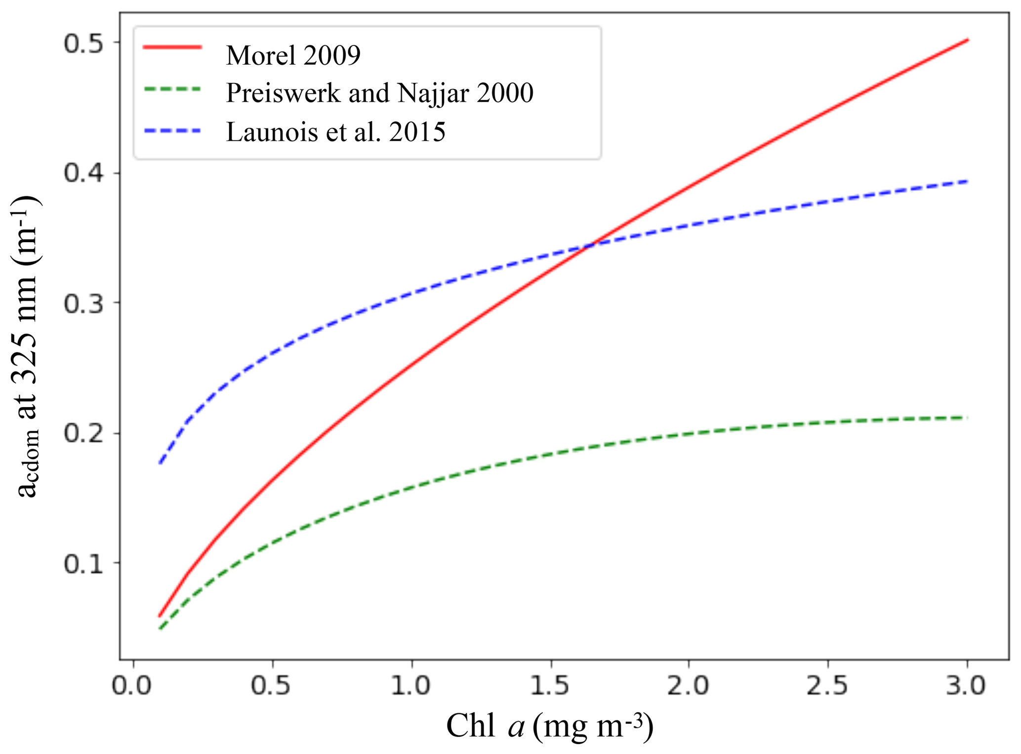
Figure 2CDOM absorption coefficient (m−1) at 325 nm as a function of the Chl a concentration (mg m−3) for the parameterizations of Morel (2009), Preiswerk and Najjar (2000) and Launois et al. (2015). The continuous line indicates the chosen parameterization.
Bacterial consumption rate
The rate of CO bacterial consumption is highly uncertain. According to experimental measurements, it seems to vary by several orders of magnitude. For example, Zafiriou et al. (2003) measured consumption rates of the order of 0.1 d−1 in the Southern Ocean, while Day and Faloona (2009) measured rates of more than 19 d−1. Hence, tests have been carried out on this rate. It is first considered constant with values ranging from 0.1 to 1.0 d−1. Secondly, it is considered to vary with the intensity of phytoplanktonic activities (proportional to Chl a) and the water temperature, according to the study of Xie et al. (2005):
with Chl the Chl a concentration (in µg L−1) and T the temperature (in ∘C). A and Y are constant parameters (0.0029 and 0.16 respectively). This equation was derived from dark incubations of 44 water samples from the Delaware Bay, Beaufort Sea and northwestern Atlantic waters in summer and autumn. The study showed a positive correlation between kCO, Chl a and temperature (R2=0.69 with μ=1). For its use in the global ocean and to reduce the mean resulting rate to 0.2 d−1, we have reduced the calculated rate kCO from the original equation of Xie et al. (2005) by multiplying by a constant μ, fitted to 0.05.
2.3 Standard experiment
The PISCES version, including the CO module, is coupled to the ocean general circulation model NEMO version 3.6. NEMO is used in an offline configuration, i.e., PISCES is run using a climatological ocean dynamical state obtained from a previous NEMO physics-only simulation (Madec, 2008). NEMO was first spun up for 200 years starting from the climatology of Conkright et al. (2002) for temperature and salinity. The last year of these dynamical fields at 5-day temporal mean resolution (ocean currents, temperature, salinity, mixed layer depth, surface radiation, etc.) was then used to force the biogeochemical model. The PISCES initial biogeochemical conditions for all tracers except CO are obtained after a 3000-year-long spin-up using the model as detailed in Aumont et al. (2015). PISCES is run for two additional years. The first year is considered as a short spin-up because of the very short lifetime of CO in the ocean, and the second year is used for the analysis presented below. The same procedure is repeated for all alternative parameterizations of the CO module, i.e., a 2-year simulation with the last year used for the analysis. Climatological atmospheric forcing fields have been constructed from various datasets consisting of daily NCEP, described in detail in Aumont et al. (2015). In particular, we are using a global climatological wind field based on the European Remote-Sensing Satellite (ERS) product and TAO observations (Menkes et al., 1998). We use the global configuration ORCA2, with a nominal horizontal resolution of 2∘ and 30 levels on the vertical (with 10 m vertical resolution in the first 200 m). Note that choosing a horizontal resolution of ∼200 km does not allow some fine-scale coastal processes to be fully resolved, such as tides or mesoscale and sub-mesoscale eddies and associated upwelling occurring in the costal ocean and hence these areas are represented with large uncertainties in the simulations performed.
2.4 Comparison to in situ data
We compiled the existing measurements of oceanic CO concentrations in order to evaluate the realism of the model results. Two types of measurements were included in this compilation: measurements of CO in the surface waters and profiles describing the concentrations as a function of depth. This dataset covers all seasons and latitudes from 80∘ N to more than 70∘ S. However, whereas the Atlantic and Pacific Ocean are fairly well covered, some wide areas are not documented (such as in the Indian ocean).
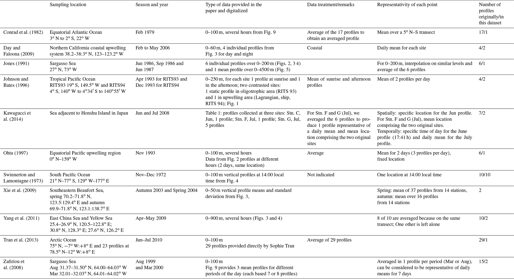
This compilation has been designed to be comparable as far as possible to the global model outputs. Indeed, as the model has a rather coarse horizontal resolution and as it does not resolve diurnal variation, we increased the spatial and temporal coverage of the data when necessary. To do so, we took the data described in the literature (which were sometimes already aggregated), and we averaged some of it. However, it is worth mentioning that averaging was not always possible and therefore after treatment each data point potentially includes a different number of observations. Tables 2 and 3 present the different datasets collected for the evaluation and the treatment we performed for the surface data (14 datasets) and for the profiles (10 datasets), respectively. After treatment, 309 surface data points and 26 vertical profiles were analyzed and compared to the model output.
Table 2Description of the observation datasets used to build the synthetic dataset of surface seawater CO concentrations.
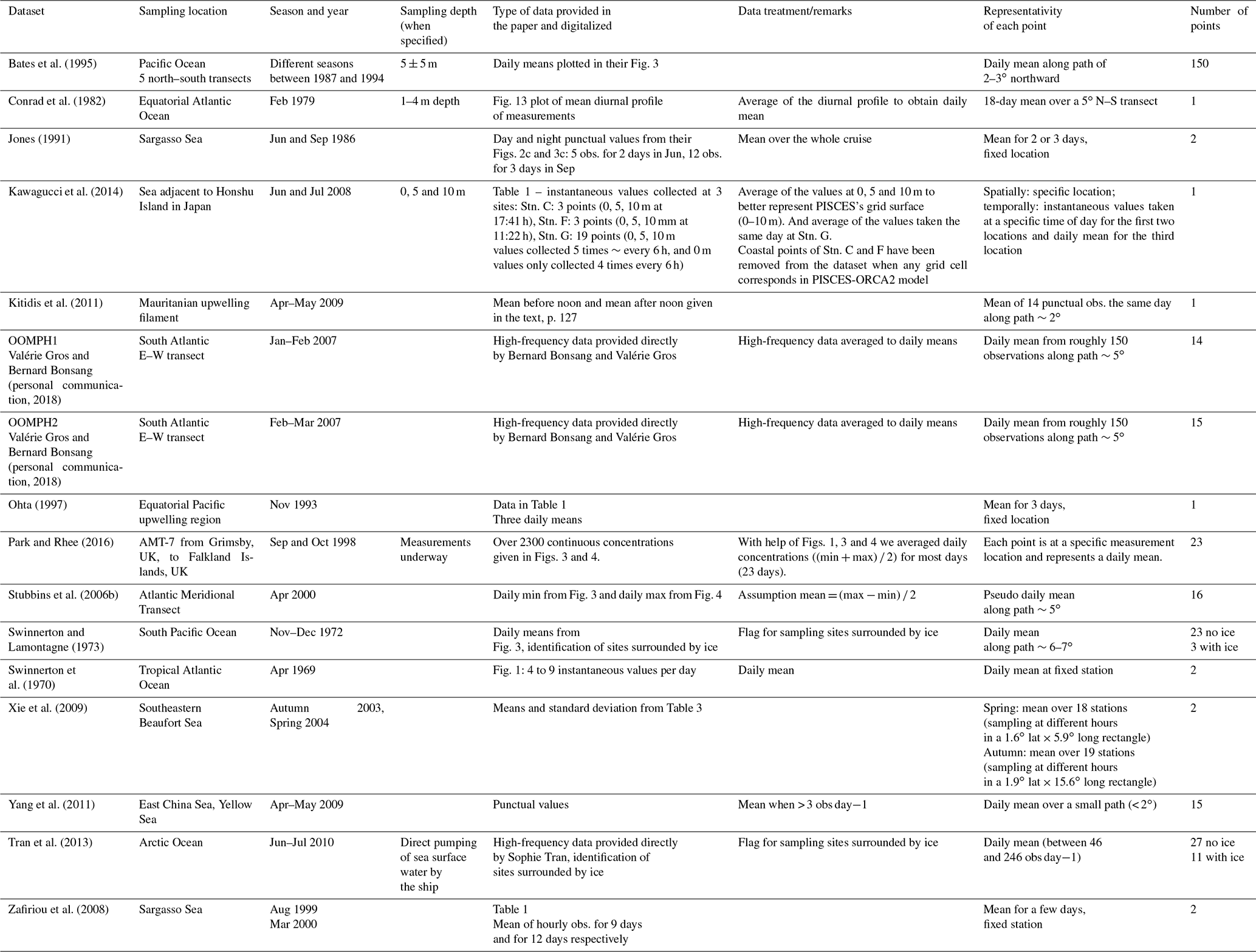
Table 3Description of the observation datasets used to build the synthetic dataset of vertical profiles of seawater CO concentrations.
For the surface data, the root mean square error (RMSE in nmol CO L−1) has also been calculated:
with N the number of observed concentrations (N=309 points).
3.1 The oceanic CO budget
In this section we describe the oceanic CO cycle as simulated by PISCES using the CO module implemented in this study. The global oceanic fluxes are first exposed. Then, the spatial patterns of the CO concentration as well as the different sources and sinks terms are presented.
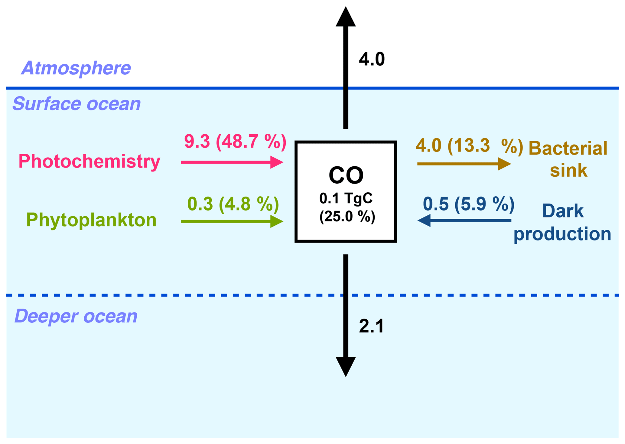
Figure 3Global fluxes in the surface ocean (between 0 and 10 m) of the oceanic CO sources and sinks (in TgC yr−1). For each biogeochemical term (photoproduction, direct phytoplankton production, dark production and bacterial consumption), the relative contribution of the surface layer to the whole water column budget is shown as a percentage.
3.1.1 Global oceanic fluxes
At the scale of the global ocean, the CO inventory is 0.4 Tg C, with a residence time of 4.3 days. The global photoproduction term in the ocean is 19.1 Tg C yr−1. It exceeds by a factor of 3 the direct phytoplankton production (6.2 Tg C yr−1) and by a factor of 2 the dark production (8.5 Tg C yr−1). The main CO sink is the bacterial consumption term (30.0 Tg C yr−1). Indeed, the global CO emission to the atmosphere (4.0 Tg C yr−1) is rather small compared to the biochemical source and sink processes. Figure 3 summarizes the values of the different terms of the CO budget in the oceanic surface layer. Only 0.1 Tg C of CO is contained in the surface layer (considered to be the first 10 m of the ocean). Almost one half of the CO photoproduction takes place in the surface layer of the ocean (9.3 Tg C yr−1 in the first 10 m), whereas only 4.8 % (0.3 Tg C yr−1) of the phytoplankton production and 5.9 % (0.5 Tg C yr−1) of the dark production unfolds there. Most of the CO produced at the surface is either emitted to the atmosphere or transported vertically towards deeper layers. The mean downward flux from the surface layer (at 10 m depth) is estimated to be 2.1 Tg C yr−1. It is therefore of the same order of magnitude as the estimated emissions to the atmosphere, which points out the importance of taking into account the effects of ocean circulation and mixing to estimate and map CO emissions.
3.1.2 Spatial patterns of the sources and sinks
Figure 4 presents the annual mean of oceanic CO concentrations and the different sources and sink terms, all vertically integrated on the first 1000 m. The integrated CO concentrations are highest at low latitudes and tend to decrease poleward. A strong CO maximum of more than 140 µmol m−2 is reached along the Equator in the central western Pacific Ocean. The integrated CO concentrations pattern is close to the dark production one, which has a strong temperature dependence and hence higher values (exceeding 5 mmol m−2 yr−1) located at the western part of the pacific basins where warm waters penetrate deeper. Integrated concentrations are also influenced by photoproduction, whose integrated values are, however, highest (exceeding 8 mmol m−2 yr−1) at the middle and western part of the basin. On the contrary, the integrated direct biological production is stronger at midlatitudes, especially in the Southern Ocean where it reaches more than 3 mmol m−2 yr−1 and is weaker in the oligotrophic gyres (around 1 mmol m−2 yr−1). The bacterial consumption term (from 0 to 12 mmol m−2 yr−1) is linearly dependent on the CO concentration and is therefore following its spatial pattern.
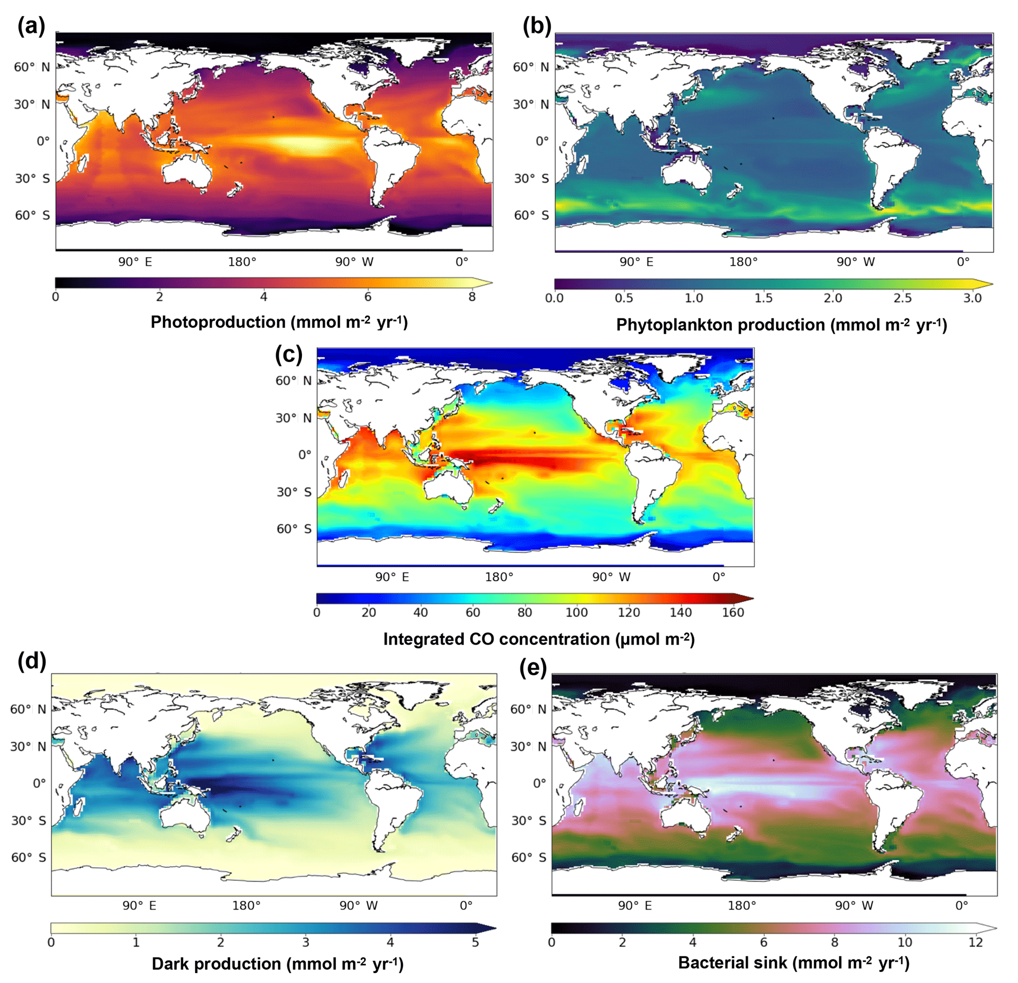
Figure 4Spatial distribution of the photoproduction (a), direct phytoplankton production (b), oceanic CO concentration (c), dark production (d) and bacterial sink (e), vertically integrated at 1000 m.
In the surface layer (taken here as the first 10 m), the patterns of the annual mean CO concentrations and the related fluxes are slightly different from the vertically integrated patterns. Figure 5 presents the annual mean surface patterns of CO concentrations and of photoproduction (panels a and c). While integrated CO concentrations patterns are influenced by the different sources and in particular the dark production, the surface patterns are very close to the surface photoproduction patterns. Indeed, concentrations are higher at the Equator, but with a strong maximum (more than 4 nmol L−1) found in the eastern equatorial Pacific Ocean. This CO maximum occurs in a highly productive area where surface waters are enriched in nutrients by the equatorial upwelling, which stretches from Galapagos Island to the South Equatorial Current and decreases westward (Wyrtki, 1981). CO is produced by an active photoproduction (up to 1.4 nmol L−1 d−1) there due to both high irradiance (more than 6 W m−2) and a high level of CDOM and is also easily concentrated in surface waters with the strong upward currents. Compared to the integrated patterns, the annual mean surface CO concentrations as well as the surface photoproduction present clear minima in the center of the subtropical gyres. Photoproduction there is around 0.5 nmol L−1 d−1 and CO concentration less than 1 nmol L−1. In the oligotrophic gyres, Chl a and hence CDOM are low, which prevents high CO photoproduction. However, light penetrates deeper allowing photoproduction to occur, even at low rate, all along the irradiated water column. In an opposite way, photoproduction in highly productive areas occurs mainly in surface waters as organic materials absorb most of the available irradiance. Figure 5b and d also present the seasonal variability of the surface patterns with latitude. Both CO and photoproduction surface patterns present a strong seasonal cycle with maximums reached at the end of spring and summer in both hemispheres.
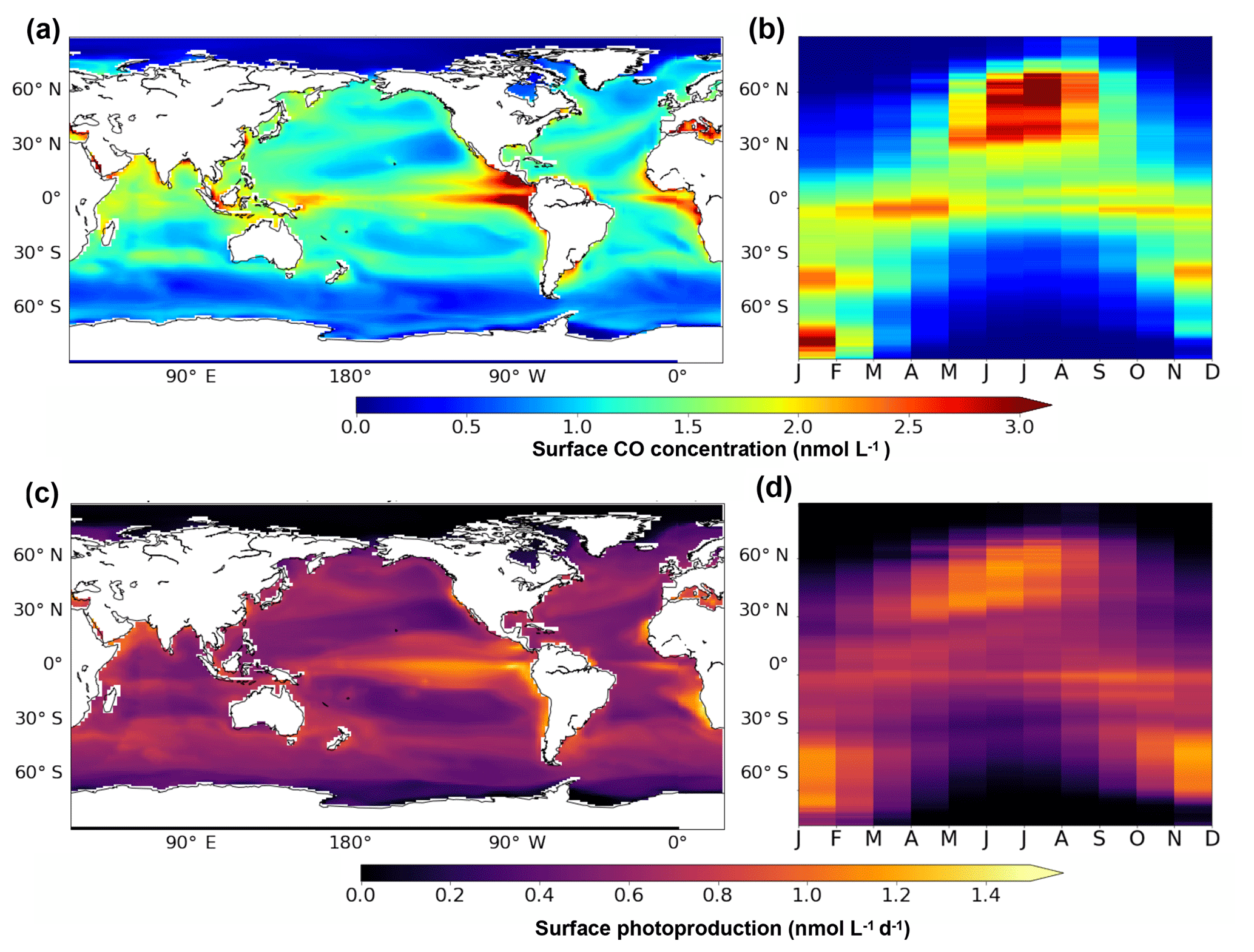
Figure 5Oceanic CO concentration (a, b) and photoproduction (c, d) between 0 and 10 m. Panels (a) and (c) present the surface spatial distribution of the annual mean. Panels (b) and (d) present the mean seasonal variation with latitude.
3.2 Evaluation of the oceanic CO concentration
Simulated surface CO concentrations have been compared to in situ concentrations, by extracting the model results collocated in time and space with measurements. A brief evaluation of simulated sea surface temperature, mixed layer depth and sea surface chlorophyll is also provided in the Supplement (Figs. S2 and S3). Note that the model simulation here is climatological so that the year of measurement cannot be taken into account for the comparisons.
3.2.1 Surface CO concentrations
Observed daily mean surface CO concentrations range from 0 to 13.9 nmol L−1 with a mean value of 2.0 nmol L−1. 75 % of the observed data are below 2.5 nmol L−1. The simulated concentrations range from 0 to 4.4 nmol L−1, with a mean of 1.6 nmol L−1 for the selected months and locations. The RMSE value resulting from the comparisons is 1.80 nmol L−1.
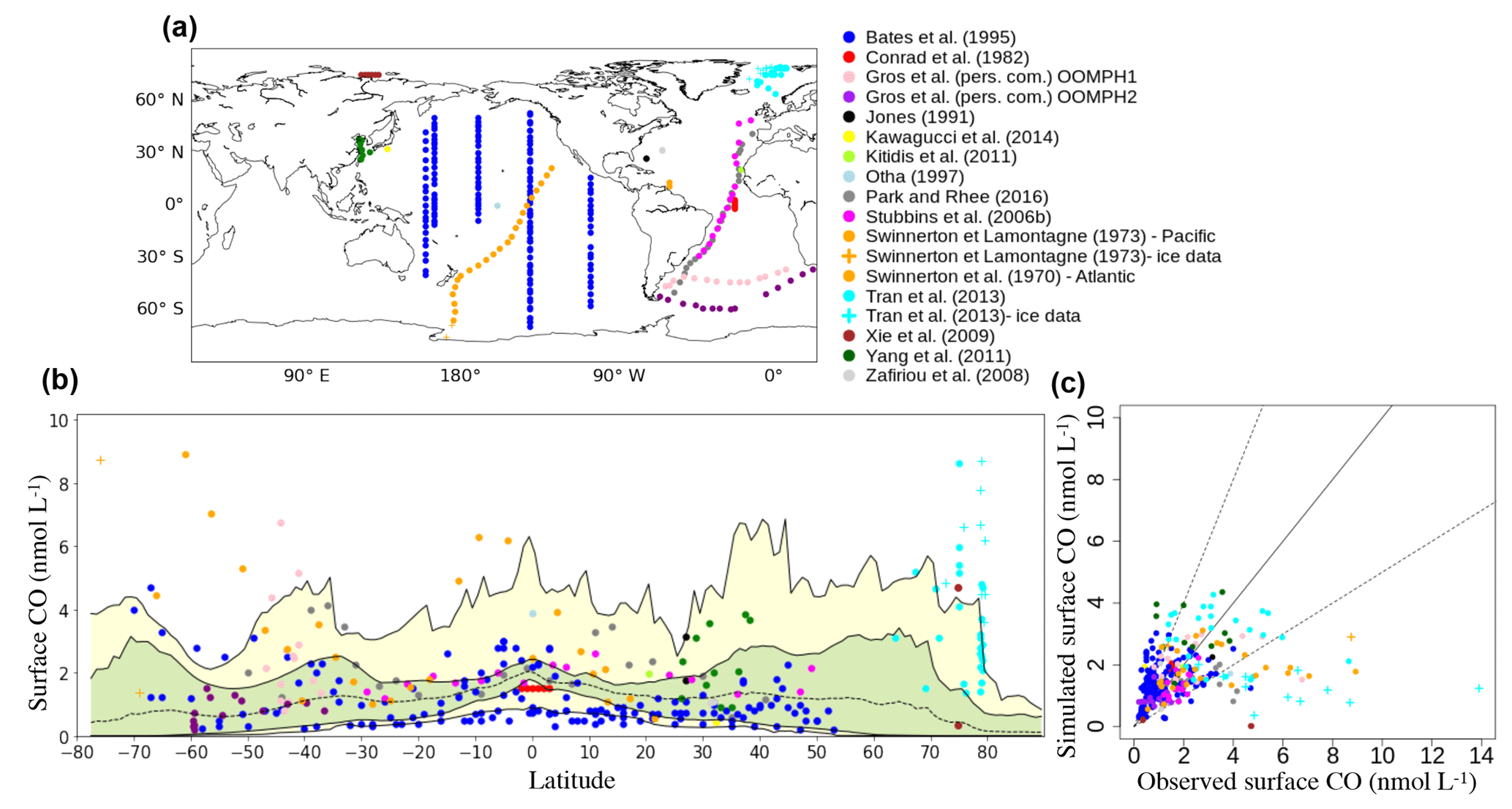
Figure 6Comparison of in situ oceanic CO concentrations between 0 and 10 m simulated with PISCES with those measured in the surface ocean. (a) Position of the surface measurements collected in the literature. (b) Surface CO concentrations as a function of the latitude (Dots: observed concentrations; dotted line: longitudinal and monthly mean simulated CO concentration; green area: interval between maximum and minimum longitudinal mean concentrations; yellow area: interval between maximum and minimum CO concentrations at a given latitude). Note that a data point of 13.9 nmol L−1 from the dataset of Tran et al. (2013) has been removed for better visibility. (c) Scatter plot the of the simulated CO surface concentrations vs. the observed concentrations. The solid line represents the 1–1 line and dotted lines the 2–1 and 2–1 lines.
Between 50∘ N and 50∘ S, the model is able to represent most concentrations within a factor of 2 (Fig. 6c). For instance, the Atlantic Meridional Transect data (Stubbins et al., 2006b) from 45∘ N to 30∘ S present rather constant surface CO concentrations around 1.5 nmol L−1 which are particularly well reproduced by the model. In the Pacific Ocean, the dataset of Bates et al. (1995) covers a broader range of latitudes and longitudes (Fig. 6a) and the model is consistent with the measured concentrations. A longitudinal gradient is observed with concentrations significantly higher in the east and central equatorial Pacific compared to the western part. Bates et al. (1995) attribute this gradient to increased biological productivity, Chl a and CDOM in the eastern upwelling region. Second, Bates et al. (1995) data show a clear latitudinal pattern, with higher concentrations from either side of the 15–30∘ S oligotrophic band (Fig. 6b). This pattern has also been highlighted by Swinnerton and Lamontagne (1973), who sampled from 20∘ N to more than 60∘ S. However, their high values at the Equator (up to 6.3 nmol L−1) are much higher than those of Bates et al. (3.0 nmol L−1). Finally, the dataset of Bates et al., which covers different periods of the year, points out the seasonal variability of the concentrations at mid-latitudes, in agreement with the photochemical nature of the main CO source.
At latitudes higher than 50∘ north or south, the model underestimates the reported high daily mean surface CO concentrations (Fig. 6b). In the Southern Ocean, simulated surface concentrations do not exceed 4.5 nmol L−1, whereas the data of Swinnerton and Lamontagne (1973), sampled in December, can reach 8.9 nmol L−1. The Southern Ocean is also the basin where Bates et al. (1995) reported their highest surface values (up to 4.7 nmol L−1). In addition, their concentration is higher for December (3.5 nmol L−1) than for March and April (0.8 nmol L−1). Therefore, the underestimation seems to occur mainly during the phytoplankton bloom season, indicating a possible bias in the CO production processes. In the Arctic, we compared simulated concentrations with the datasets of Xie et al. (2009) and Tran et al. (2013). Xie et al. (2009) measured, in the open waters of the southeastern Beaufort Sea, a mean CO concentration of only 0.4 nmol L−1 in autumn, which is particularly well represented by the model. However, their higher mean value of 4.7 nmol L−1 during the spring season is highly underestimated, indicating once again a possible bias with the CO production processes. Tran et al. collected samples in July 2010 between Svalbard, Greenland and Iceland. Closer to the Norwegian basin, measurements have been performed in open-ocean water. It presents a high variability there (from 1.4 to 8.7 nmol L−1), but most data points are under 4.0 nmol L−1 and represented within a factor of 2 by the model. Closer to the Greenland shelf, measurements have been performed in polar waters where pack ice was present. In this area, measured surface concentrations are significantly higher (up to 13.9 nmol L−1) and are clearly underestimated by the model. Other studies have measured high surface CO concentrations in polar regions (Xie and Gosselin, 2005; Valérie Gros, personal communication, 2018), which tends to strengthen the conclusion that major mismatches between our modeled and the observed CO concentrations occur in that region. Indeed, Valérie Gros (personal communication, 2018) measured, north of Svalbard, a mean concentration of 7.1 nmol L−1 in May 2015. These high CO concentrations reported in polar regions could be due to the release of organic matter in the open ocean during ice melting due to algae growing in the ice (Belzile et al., 2000). It could also be due to the direct release of CO produced inside the ice. Indeed, Xie and Gosselin (2005) mentioned that sea ice is a suitable matrix for efficient photoreactions involving CDOM, and measured concentrations in May exceeding 100 nmol L−1 in the bottom layer of a few first-year sea-ice cores sampled in the southeastern Beaufort Sea. However, according to Xie et al. (2009) and Zafiriou et al. (2003), the high CO concentrations reported at high latitudes may be mainly due to slower microbial CO uptake rates in cold waters. Indeed, Zafiriou et al. estimated rates as low as 0.09 d−1 in the Southern Ocean.
It is the first time that such a dataset of in situ CO concentrations in the surface ocean have been gathered and that a 3-D global biogeochemical model is used to simulate the oceanic CO cycle. Despite the scarcity of measurements regarding space and time, PISCES reproduces the observed surface concentrations reasonably well, at least for the open ocean between 50∘ N and 50∘ S. While concentrations at low latitudes and midlatitudes are simulated within a factor of 2, photoproduction or consumption processes might not be well represented at high latitude.
3.2.2 Vertical CO profiles
In this section, we evaluate the vertical distribution of CO concentrations as simulated by PISCES against available observed vertical profiles. Only 10 available profiles out of 26 are shown hereafter (Fig. 7), covering different types of marine environments. Other profiles are available in the Supplement.
All simulated CO profiles exhibit a decrease with depth. They are mainly driven by the photoproduction source, which is a combination of the CDOM and irradiance levels. Indeed, no clear subsurface maximums, potentially associated with direct phytoplankton production, are seen. This is also the case for the observed profiles. At 100 m, simulated as well as observed concentrations reach values close to zero, explained by the negligible influence of light irradiance under these depths. However, the shapes of the decreases differ with time and location, which can be related both to differences in the light penetration and mixed layer depths.
When trying to compare simulated and observed profiles one by one, we observe quantitative differences. When the model is able to correctly simulate the concentration at the surface, the deeper concentration is also well simulated. On the contrary, when the model overestimate or underestimate the surface concentration, it is also the case below (see as an example the representation of the two profiles of Zafiriou et al., 2008 taken in the Sargasso Sea in March and August). Nevertheless, the model is always in good agreement with the nearly zero concentrations below 100 m. It is, however, particularly hard to bring out spatial or temporal trends for the observed underestimations or overestimations. As an example for the equatorial Pacific region, the model underestimates by a factor of 2 the concentrations of Johnson and Bates (1996), whereas in the same region in November the data of Ohta (1997) are well represented. Additionally, it is worth mentioning that high variability and uncertainty is associated with some measurements. For example, Yang et al. (2011) measured spring month concentrations of 0.0 to 7.5 nmol L−1 between 25 and 50 m in the Coastal East China and Yellow seas. Also, when no standard deviation is available the data reflect one-time measures. In particular, this is the case for the 10 profiles of Swinnerton and Lamontagne (1973), taken during early afternoon. It is hence difficult to compare these profiles with monthly averaged model outputs.
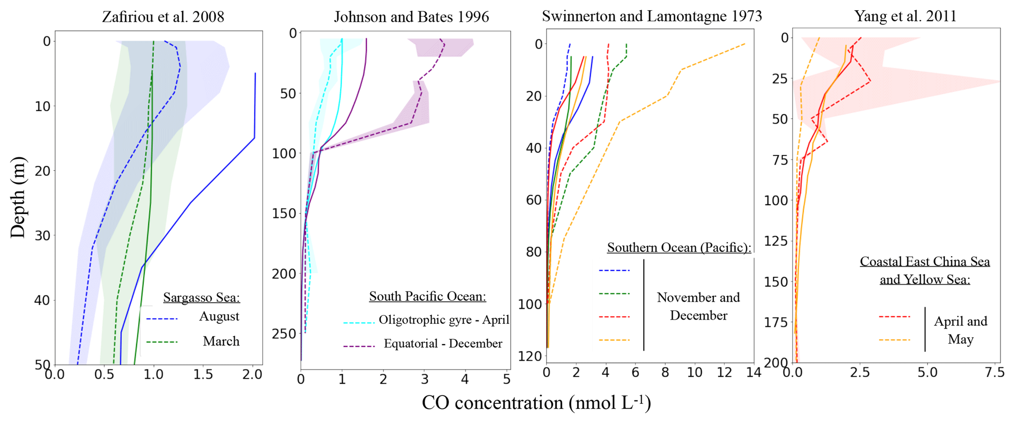
Figure 7Comparison of simulated oceanic CO profiles with the measured profiles (simulated profiles for the same months and location as measurement). Only a few datasets are shown in this figure (others are available in the Supplement). Dotted lines represent the observed profiles and continuous lines the model output. The standard deviation of the observation, when available, is shown around each observed profile with the shaded area of the same color.
3.3 Sensitivity to alternative parameterizations
Alternative parameterizations have been tested regarding the CDOM estimation (affecting photoproduction and dark production) and the bacterial consumption term.
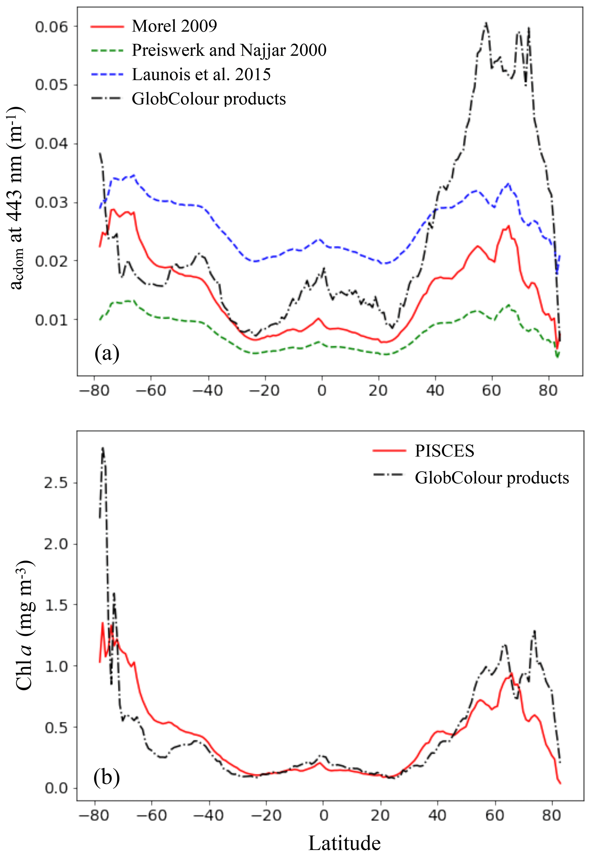
Figure 8Comparison of the CDOM absorption coefficient at 443 nm (a) and Chl a (b) simulated by PISCES with GlobColour products averaged over 2002–2012, as a function of latitude. For the CDOM absorption coefficient, the different parameterizations tested are shown.
3.3.1 CDOM parameterization
Surface CDOM absorption. Different parameterizations for the CDOM absorption coefficient have been tested, all using the same simulated Chl a concentrations. The latitudinal mean of these coefficients, taken at 443 nm and for the surface ocean, are shown in Fig. 8 and compared to the mean climatology of CDM (colored detrital matter) distributed within the GlobColour products (Maritorena et al., 2010; Fanton d'Andon et al., 2009), averaged over 2002–2012 (a). As all CDOM parameterizations depend on Chl a concentrations, Fig. 8 also shows the latitudinal mean of the Chl a (b), simulated by PISCES and distributed within the GlobColour products, in order to better separate the respective roles of the CDOM parameterization versus Chl a representation. Additional Chl a comparisons with satellite products are also available in the Supplement (Fig. S2). All CDOM parameterizations lead to similar distributions, with higher values at high latitudes, intermediate values near the Equator and the lowest values in the subtropical gyres, as is the case for Chl a surface concentrations. However, the magnitudes of these CDOM absorption coefficients are very different and vary within a factor of 3 across the different parameterizations. The magnitude from the parameterization of Morel (2009), chosen for our standard simulation, gives intermediate values (global mean is 0.014 m−1) between Preiswerk and Najjar (mean 0.008 m−1) and Launois et al. (mean 0.026 m−1). The GlobColour CDM content can be considered as a proxy for CDOM as it has been postulated that the CDOM absorbance represents 90 % of the CDM absorbance (Siegel et al., 2002). Latitudinal variations are consistent between the satellite products and the tested parameterizations. Minima (less than 0.01 m−1) are located in oligotrophic gyres. Quantitatively, those minima are best represented by the relation of Morel, since those of Launois et al. (2015) and of Preiswerk and Najjar (2000) give too high and too low values, respectively. The highest satellite-derived CDM absorptions are reached at high latitudes, especially in the Northern Hemisphere (latitudinal mean goes up to 0.060 m−1 between 50 and 80∘ N). These high CDM values correspond mainly to coastal areas, and none of the parameterizations tested here are able to reproduce them. Because the Chl a concentration is rather well represented in the Northern Hemisphere compared to satellite-derived Chl a (Figs. 8 and S2), this strong underestimation is attributable to the CDOM parameterization itself. Indeed, the different parameterizations are all depending on Chl a and are therefore probably better suited for Case-1 waters (Matsushita et al., 2012), for which most dissolved organic matter comes from local phytoplanktonic activities like cell lyses, exsudation or grazing (Para et al., 2010). Indeed, the CDOM concentration in coastal waters is also regulated by the interactions with the continent (Bricaud et al., 1981; Siegel et al., 2002), especially at river mouths where CDOM concentrations are generally higher than for the rest of the ocean (Para et al., 2010). This is the consequence of a local stimulation of primary production associated with nutrient supply (Carder et al., 1989), but also of a direct supply of continental CDOM (Nelson et al., 2007). This direct CDOM supply is not represented in the model, potentially leading to an underestimation of the CO photoproduction in coastal areas, and potentially also in open ocean waters under terrestrial influence. This is particularly the case for the Arctic Ocean as it is enriched in terrestrial dissolved organic matter due to high river supply (Dittmar and Kattner, 2003). Additionally, this could explain part of the CO underestimations in the Arctic, together with the aforesaid mechanism associated with the presence of sea ice. In the Southern Ocean, the CDOM content is slightly above the CDM content retrieved from space (except at the very close Antarctic coast). This could be due to the Chl a overestimation in that region (Figs. 8 and S2). However, whereas Chl a is overestimated, CO underestimations were observed. Hence, to explain CO underestimations, in this region it is better to opt for a link with the representation of the bacterial consumption term. Finally, among the three parameterizations, we chose the one of Morel (2009) for our representation of the CDOM absorption despite the underestimations in the Northern Hemisphere, because globally it fits the satellite-derived CDM better as the amplitude of the latitudinal gradient is the largest (standard deviation is 0.007 m−1, compared to 0.005 m−1 for Launois and 0.003 m−1 for Preiswerk and Najjar relations). Nevertheless, it is important to mention that CDOM is very heterogeneous matter and therefore using Chl a as a proxy for CDOM is in any case obviously reductive, as CDOM has its own dynamic.
Sensitivity of the oceanic CO budget to changes in the CDOM parameterization. Global fluxes have been calculated from the simulations using the different CDOM parameterization (Table 1, lines 1–3). The global photoproduction flux is more than doubled when using the parameterization of Launois et al. (49.1 Tg C yr−1 compared to 19.1 Tg C yr−1 when using that of Morel) and decreases with the one of Preiswerk and Najjar (14.2 Tg C yr−1), in agreement with the quantitative tendencies of the CDOM surface values discussed above. In a similar way, the global dark production flux is more than tripled when using the parameterization of Launois et al. (29.5 Tg C yr−1 compared to 8.5 Tg C yr−1 when using that of Morel) and reduced with that of Preiswerk and Najjar (7.2 Tg C yr−1). For these different tests, the bacterial consumption rates have been kept the same so that the changes in the CO budget and in other terms are solely due to changes in photoproduction and dark production. The CO flux to the atmosphere (3.0–10.2 Tg C yr−1) and the bacterial sink (24.7–74.7 Tg C yr−1) both vary accordingly with the changes in photoproduction and dark production. As a direct consequence, the oceanic CO total inventory is modified (0.3–1.0 Tg C), which also changes the values of the RMSE when comparing simulated surface CO concentrations with in situ measurements (it is 2.91 nmol L−1 with Launois et al. and 1.91 nmol L−1 with Preiswerk and Najjar, whereas it is 1.80 nmol L−1 with Morel). Note that the direct phytoplankton production term remains the same as it does not depend on CO concentrations. Photoproduction has also been integrated in the mixed layer in order to be compared to the value of 39.3 Tg C yr−1 computed by Fichot and Miller (2010) with a global model using ocean color data for the CDOM parameterization. With a budget of 45.4 Tg C yr−1, the photoproduction of Launois et al. gives the closest estimation, those resulting from Morel and from Preiswerk and Najjar being much lower (17.7 and 13.1 Tg C yr−1 respectively). Those two latter estimations are also lower than the most recent estimations based on extrapolations of in situ measurements. Indeed, Zafiriou et al. (2003) estimated the photoproduction between 30 and 70 Tg C yr−1 based on a large dataset collected in the Pacific Ocean and Stubbins et al. (2006b) estimated it between 38 and 84 Tg C yr−1 with Atlantic Ocean data. For the dark production, the use of the CDOM parameterizations of Morel on the one hand and Preiswerk and Najjar on the other hand give global values in the range of previous estimates (4.9–15.8 Tg C yr−1; Zhang et al., 2008), whereas Launois et al.'s resulting estimate is much higher (29.5 Tg C yr−1).
3.3.2 CO consumption
Several simulations regarding the bacterial consumption have been performed. First, different values for a constant bacterial rate have been tested. Second, a variable rate as a function of Chl a and temperature according to the relation of Xie et al. (2005) has also been tested. Global budgets resulting from these different tests are shown in Table 1 (lines 4–8), using the same CDOM parameterization (Morel, 2009) so that the impact of the photo and dark productions terms on the oceanic CO concentration remains the same. When increasing the rate from 0.1 to 2.0 d−1 (with a constant value), the bacterial sink increases from 27.5 to 33.9 Tg C yr−1. This rise of consumption induces a strong decrease in the CO inventory (from 0.8 to 0.04 Tg C) and therefore also decreases the flux to the atmosphere (from 6.4 to 0.5 Tg C yr−1). When changing the rate, the fit of the surface CO concentration with observations is also modified. Indeed, when it is 0.1 d−1, the RMSE value is increased (= 1.97 nmol L−1) compared to the control run (RMSE=1.80 nmol L−1) because of an overall overestimation of CO concentrations. When the consumption rate exceeds 0.2 d−1, the RMSE value is also increased but this time because of an overall underestimation. For the test using a spatiotemporally varying rate (Table 1, line 8), we slightly modified the initial equation of Xie et al. (2005) by adding a factor μ=0.05, so that the mean kCO is 0.2 d−1. Indeed, when using the original μ=1 with our model, bacterial rates vary from 3.8 to 7.0 d−1 and thus lead to a strong underestimation of CO concentrations. When a varying rate is applied, the global bacterial sink, the CO inventory and the CO flux to the atmosphere are pretty much the same as using the standard run with a constant rate of 0.2 d−1. Also, the RMSE value is almost identical (1.79 nmol L−1). Thus, applying this varying rate did not help to improve the fit of CO concentrations against in situ measurements, which could be explained by the very low standard deviation of the resulting kCO values (0.01 d−1).
Being the main CO sink in the ocean, a more accurate parameterization of the bacterial CO consumption term is essential to quantify CO emissions to the atmosphere. However, little is known on the CO bacterial consumption, although it has been shown to be ubiquitous in diverse marine ecosystems, particularly in the northeastern Atlantic and Arctic waters (Xie et al., 2005, 2009). According to Xie et al. (2005), this process could follow different patterns from first- to zero-order kinetics or saturation, but most marine waters may be reasonably well approximated by the first-order kinetic, as CO concentrations rarely exceed the half-saturation constant value. It is nevertheless difficult to constrain the bacterial consumption rate based on experimental estimations, as they present a very high variability. The highest rates seem to be found for coastal waters, suggesting the presence of active CO oxidizing communities (Tolli et al., 2006; Tolli and Taylor, 2005). For example, Day and Faloona (2009) measured rates from 1.2 to 19.2 d−1 along the Californian coasts and Jones and Amador (1993) rates from 0.2 to 12 d−1 in the Caribbean Sea. In the remote ocean, measured rates are lower but the variability remains high. Zafiriou et al. (2003) measured a rate as low as 0.1 d−1 in the Southern Ocean, whereas Conrad et al. (1982) retrieved values around 0.7 d−1 in the equatorial Atlantic and Ohta (1997) more than 3.0 d−1 in the equatorial Pacific. Part of this high variability might be explained by the fact that, as for other microbial processes, the CO consumption should also depend on a number of parameters like microbial species, productivity, temperature or ocean acidity (Xie et al., 2005). Using the only study proposing to compute the kCO value with Chl a and temperature (Xie et al., 2005), we attempted to account for this variability. However, it seems that such an empirical equation, developed with data from the Delaware Bay, the northwestern Atlantic and the Beaufort Sea, is not suitable for a global application as it leads to very high kCO values. Even when tuning with the factor μ, the remaining kCO variability is too small to significantly improve the fit with the observed surface CO concentrations.
Based on these different tests, we show that the main terms controlling oceanic CO concentrations are still largely under-constrained, although available in situ CO concentrations, global budget estimates and the CDM concentrations retrieved from space are helping in the choice of standard, i.e., “best guess” simulation. Here, the best parameterization of CDOM absorption compared to satellite products is given by Morel (2009), which then dictates our choice for the standard simulation. However, it is worth mentioning that using the parameterization of Launois et al. (2015) with a higher bacterial consumption rate, or the one of Preiswerk and Najjar (2000) with lower consumption rate, would result in oceanic CO concentrations that give similar skill scores when compared to available CO concentration observations (tests not shown), but for which we have less confidence in the CDOM parameterization.
3.4 Simulated CO emissions
This section first presents the CO emissions to the atmosphere resulting from our standard simulation. Then, the emissions are compared to the canonical distribution of CO emissions published by Erickson (1989), which is the only gridded global CO emission dataset available to date in the literature.
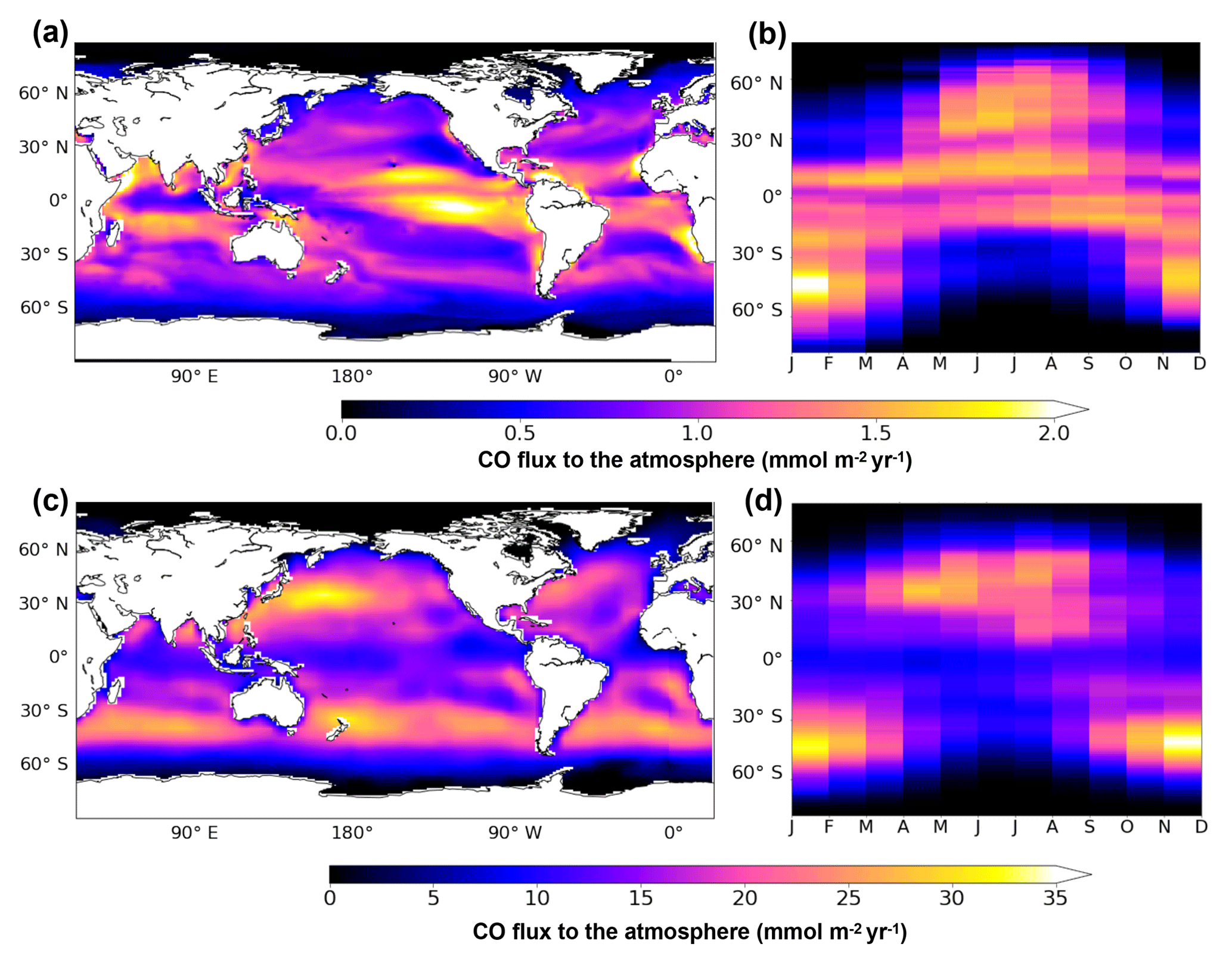
Figure 9Oceanic CO emissions simulated by PISCES (a, b) or by the model of Erickson (1989) (c, d). Panels (a) and (c) present the spatial distribution of annual mean emissions. Panels (b) and (d) present the mean seasonal variation with latitude. All fluxes are in mmol m−2 yr−1 and are directed toward the at mosphere.
Figure 9a presents the spatial patterns of emissions resulting from PISCES. All oceanic regions are net sources of CO for the atmosphere, with emissions varying spatially from 0 to 2.6 mmol m−2 yr−1 on an annual mean basis with a global mean flux of 0.8 mmol m−2 yr−1. The spatial pattern of emissions follows the one of the surface CO concentrations. The strongest emissions are simulated in the equatorial region, especially in the east Pacific Ocean on both sides of the Equator. High emissions are also reached locally along the west coast of South America and Africa. Annual mean emissions are reduced to roughly 0.5 mmol m−2 yr−1 in the center of the subtropical gyres and to almost zero at latitudes higher than 60∘. Simulated CO emissions also present a strong seasonal variability (Fig. 9b). While emissions at the Equator (30∘ S–30∘ N) are roughly constant throughout the year (around 1.5 mmol m−2 yr−1), emissions at intermediate latitudes (30 to 60∘) vary seasonally from 0 to the highest values encountered (up to 2.0 mmol m−2 yr−1). However, on a yearly basis, the equatorial region is the major contributor with a flux of 2.5 Tg C yr−1, which is more than 60 % of the global value (4.0 Tg C yr−1). Intermediate latitudes contribute to 1.4 Tg C yr−1 and polar regions (more than 60∘ N and S) to only 0.1 Tg C yr−1. Additionally, emissions are stronger in the Southern Hemisphere than in the Northern Hemisphere (2.3 and 1.7 Tg C yr−1 emitted respectively), which could be attributable to the larger surface area covered by oceans and to the slightly closer proximity of the Earth to the Sun during the southern summer solstice. Finally, our global emission of 4.0 Tg C yr−1 simulated with PISCES falls well into the range of previous estimations based on extrapolations from in situ oceanic CO measurements. From Atlantic data, Stubbins et al. (2006a) estimated a yearly flux to the atmosphere of 3.7±2.6 Tg C yr−1 and Park and Rhee (2016) estimated the emissions in the range 1–12 Tg C yr−1. From Pacific data, Zafiriou et al. (2003) estimated a flux of 6 Tg C yr−1 and Bates et al. (1995) a range of 3–11 Tg C yr−1.
The CO emissions produced by Erickson (1989) are still currently used as spatial distribution by global chemistry-climate models. They are presented here as published in 1989, but are now generally rescaled to lower total emissions for use in atmospheric models. Figure 9c and d present the spatial patterns and seasonal variability of emissions resulting from Erickson's model, respectively. In agreement with our simulation, all oceanic regions are sources of CO for the atmosphere. However, emissions present very large spatial and quantitative differences. On an annual mean basis, Erickson's emissions vary from 0 to more than 33 mmol m−2 yr−1 (mean is 9.0 mmol m−2 yr−1), which is 1 order of magnitude above those of PISCES. The emission pattern for Erickson clearly presents two bands of intense outgassing at midlatitudes (between 30 and 60∘ N and S), whereas the pattern for PISCES presents maxima around the equatorial zone and minima in the center of the oligotrophic gyres. When looking at the seasonal variability, Erickson's model also simulates the highest emissions at midlatitudes in summer months but with much stronger maximum values (up to 40 mmol m−2 yr−1). Globally, Erickson's model produces a flux of 70.7 Tg C yr−1, which is 20 times greater than the PISCES estimation. PISCES flux is therefore much closer to the most recent estimations (Stubbins et al., 2006a; Zafiriou et al., 2003; Bates et al., 1995).
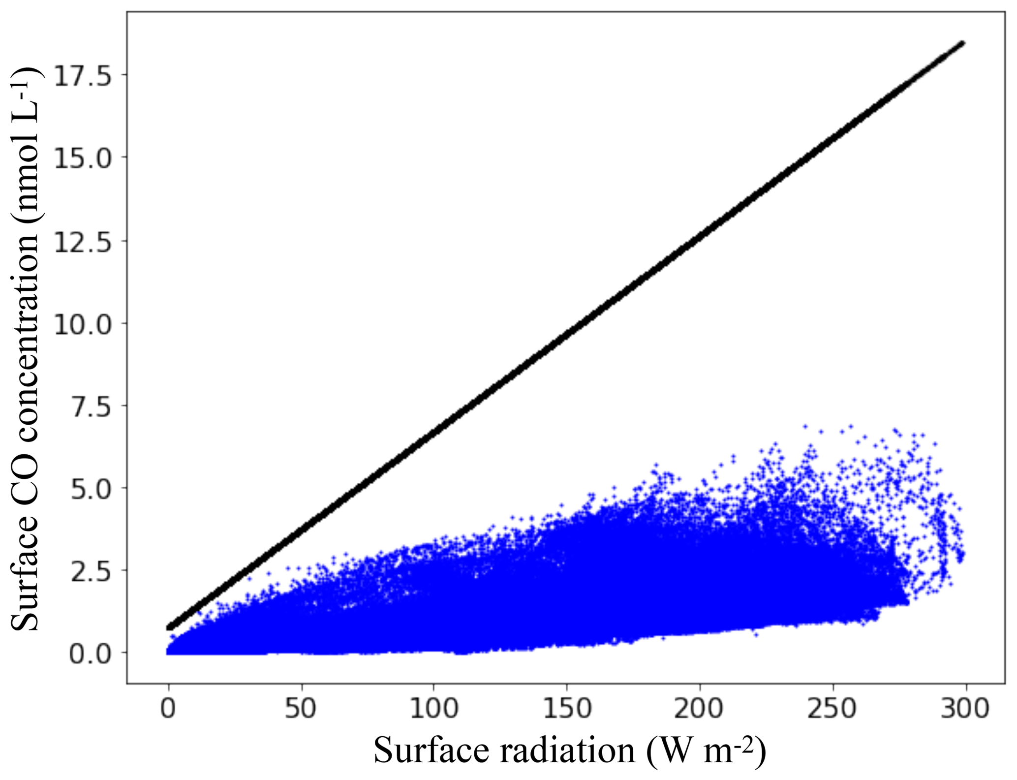
Figure 10Surface CO concentrations as a function of the total solar radiation available at the surface ocean. Blue dots are mean annual surface concentrations retrieved from PISCES and the black line is the linear relation used by Erickson (1989).
The spatial and quantitative differences between Erickson's and PISCES's emissions are mainly attributable to the fact that the biochemical processes known to control the CO concentration at the surface ocean are not accounted for in the Erickson's representation. In a similar way to Eq. (15) of PISCES, the emissions of Erickson depend on the CO concentration gradient between the atmospheric and oceanic parts. However, the oceanic part is not computed dynamically and linearly depends on the total available radiation at the surface ocean based on a relation derived empirically with Atlantic data of Conrad et al. (1982). Figure 10 shows the mean annual surface CO concentrations as a function of the mean annual total solar radiation in PISCES, as well as the linear relation used by Erickson. Mean surface radiation in PISCES ranges from 0 to 300 W m−2 and the stronger it is, the higher the concentrations for both models. However, for the same given radiation there is in PISCES a multitude of possible values for the CO concentration, as it is controlled by different processes (light, CDOM content, Chl a, bacterial consumption) and not only by the light intensity. As a result, the mean annual surface concentrations do not exceed 6.6 nmol L−1, whereas it can reach 18.0 nmol L−1 with 300 W m−2 with the Erickson's relation. Values reached by Erickson's model are therefore much higher and this implies stronger outgassing to the atmosphere. It is worth mentioning that given the in situ measurements of surface CO concentrations presented in Sect. 3.2, the relation of Erickson would easily overestimate the concentrations for the regions with high radiation.
We used a global 3-D biogeochemical model to explicitly represent the oceanic CO cycle based on the up-to-date knowledge of its biochemical sources and sinks. With our best-guess modeling setup, we estimate a photoproduction of 19.1 Tg C yr−1, a dark production of 8.5 Tg C yr−1, a phytoplanktonic production of 6.2 Tg C yr−1 and a bacterial consumption of 30.0 Tg C yr−1. The estimation of the CO flux to the atmosphere is 4.0 Tg C yr−1 and falls well into the range of previous recent estimates (Stubbins et al., 2006a; Zafiriou et al., 2003; Bates et al., 1995). The global downward flux at 10 m depth, estimated at 2.1 Tg C yr−1, points out the importance of taking into account the effects of ocean circulation and mixing to model the oceanic CO cycle and the interplay between source and sink processes and emissions to the atmosphere.
The distribution of surface CO concentrations primarily reflects the distribution of CDOM in the surface ocean and its impact on the photoproduction source, with high concentrations of CO in the biologically productive regions of the ocean. For the first time, a large dataset of in situ CO measurements collected from the literature has been gathered and used to evaluate these concentrations. Despite the scarcity of these measurements in terms of their spatial and temporal distribution, the proposed best simulation is able to represent most of the ∼300 data points within a factor of 2.
That said, there are a number of limitations that probably preclude a better agreement between our model and the available data:
- i.
Regarding the spatial scale, our simulated concentrations are probably impacted by the very coarse resolution of the model. In particular, this is critical to resolving the coastal ocean, where a number of in situ measurements of CO concentrations have been performed. Indeed, the ∼100-to-200 km horizontal resolution does not allow some fine-scale coastal processes to be fully resolved, and hence our estimation of the oceanic CO cycle is rather suitable to the blue waters, although a crude representation of specific processes occurring in coastal areas exists (like riverine nutrients inputs, iron input by sediment resuspension or coastal upwellings).
- ii.
Regarding the temporal scale, the model does not explicitly resolve the diurnal cycle although the variations in surface CO concentrations during the day have been shown to be first-order variations (Carpenter et al., 2012). In addition, the model does not consider the inter-annual variability of ocean physics and biogeochemistry, as it is forced by a climatology of surface fields (temperature, winds, precipitation, etc.) (Aumont et al., 2015). This might be limiting for the evaluation of the simulated CO concentrations against in situ measurements, as it has not been always possible to average the data in order to be representative of daily means, and as the data are covering 50 years of measurement during which atmospheric forcing might have changed.
- iii.
In addition, we note a rather clear underestimation of the simulated CO concentrations when compared to in situ measurements at high latitudes. This may result from a lower bacterial consumption rate in these regions and/or from higher CDOM levels associated with the presence of sea ice or to riverine input of organic matter. Neither the supply of CDOM by sea ice nor by rivers is represented in the model, which may prevent an accurate representation of the CO cycle in those regions.
We also want to emphasize the large uncertainties associated with the different terms, in particular to the main CO source: photoproduction. Indeed, we have shown that the global photoproduction can vary within a factor of 3 (14.2–49.1 Tg C yr−1) depending on the CDOM parameterization chosen. Efforts should be focused toward a better understanding of the complex CDOM nature and on its representation in models, especially as good knowledge of its spatiotemporal distribution is critical not only for the CO production but also for a better understanding of remineralization of dissolved organic carbon in the ocean (Mopper and Kieber, 2001), and more generally of the biogeochemical cycles that are driven by light availability in the ocean (Shanmugam, 2011). Beyond a better knowledge of the CDOM pool, it must be mentioned that the whole organic matter pool needs to be better understood in order to better constrain photoproduction. Indeed, it has been suggested that even particulate organic matter could be a substrate for CO photoproduction (Xie and Zafiriou, 2009).
Finally, we compared our estimates of ocean CO emissions to those published by Erickson (1989). Our emissions are quantitatively much closer to the most recent estimates and in better agreement in terms of spatial distribution with the known processes controlling the oceanic CO. Future works will assess the impact of our estimates of CO emissions on the oxidizing capacity of the atmosphere with respect to that obtained with the canonical Erickson's estimates. Besides, the implementation of our ocean CO cycle module within an Earth system model will enable the exploration of potential Earth system feedbacks associated with the oceanic CO cycle.
Data (model output) are available at https://doi.org/10.17882/59311 (Conte et al., 2019).
The supplement related to this article is available online at: https://doi.org/10.5194/bg-16-881-2019-supplement.
The author contributions to this paper are as follows.
-
Conceptualization: SS and LB
-
Data curation: SS
-
Formal analysis: LC
-
Funding acquisation: SS and LB
-
Investigation: all
-
Methodology: all
-
Validation: LC
-
Visualization: LC
-
Writing original first draft: LC
-
Writing, review: all
The authors declare that they have no conflict of interest.
We would like to thank the LEFE FORCAGE and EU-H2020-CRESCENDO (grant
agreement no. 641816) projects for funding. We also gratefully acknowledge
Valérie Gros and Bernard Bonsang for their contribution and access to CO
data from their TRANSSIZ and OOMPH cruises. The first version of the work was
performed during the internship of Aïda Bellataf in 2012 with the help
of Sophie Tran. The authors are thankful to them and our thoughts are with
Aïda, a very dynamic and enthusiastic student whose life was brutally
cut short in 2017 at the age of 32. Finally, we thank the GlobColour project
for providing access to the CDM content (http://globcolour.info, last
access: 12 February 2019) and the ASTM for the distribution of the
ground-based solar spectral irradiance SMARTS2 (version 2.9.2) Simple Model
for Atmospheric Transmission of Sunshine
(https://www.astm.org/Standards/G173.htm, last access:
12 February 2019).
Edited by: Tina
Treude
Reviewed by: two anonymous referees
ASTM G173-03: Standard Tables for Reference Solar Spectral Irradiances: Direct Normal and Hemispherical on 37∘ Tilted Surface, ASTM International, West Conshohocken, PA, available at: https://www.astm.org (last access: 12 February 2019), 2012.
Aumont, O., Ethé, C., Tagliabue, A., Bopp, L., and Gehlen, M.: PISCES-v2: an ocean biogeochemical model for carbon and ecosystem studies, Geosci. Model Dev., 8, 2465–2513, https://doi.org/10.5194/gmd-8-2465-2015, 2015.
Bates, T. S., Kelly, K. C., Johnson, J. E., and Gammon, R. H.: Regional and seasonal variations in the flux of oceanic carbon monoxide to the atmosphere, J. Geophys. Res., 100, 23093, https://doi.org/10.1029/95JD02737, 1995.
Belzile, C., Johannessen, S. C., Gosselin, M., Demers, S., and Miller, W. L.: Ultraviolet attenuation by dissolved and particulate constituents of first-year ice during late spring in an Arctic polynya, Limnol. Oceanogr., 45, 1265–1273, 2000.
Bricaud, A., Morel, A., and Prieur, L.: Absorption by dissolved organic matter of the sea (yellow substance) in the UV and visible domains1, Limnol. Oceanogr., 26, 43–53, https://doi.org/10.4319/lo.1981.26.1.0043, 1981.
Bullister, J. L., Guinasso, N. L., and Schink, D. R.: Dissolved hydrogen, carbon monoxide, and methane at the CEPEX site, J. Geophys. Res., 87, 2022, https://doi.org/10.1029/JC087iC03p02022, 1982.
Carder, K. L., Steward, R. G., Harvey, G. R., and Ortner, P. B.: Marine humic and fulvic acids: Their effects on remote sensing of ocean chlorophyll, Limnol. Oceanogr., 34, 68–81, 1989.
Carpenter, L. J., Archer, S. D., and Beale, R.: Ocean-atmosphere trace gas exchange, Chem. Soc. Rev., 41, 6473, https://doi.org/10.1039/c2cs35121h, 2012.
Cicerone, R. J.: How the Concentration of Atmospheric CO changed?, The Changing Atmosphere, 49–61, 1988.
Conkright, M. E., Locarnini, R. A., Garcia, H. E., O'Brien, T. D., Boyer, T. P., Stephens, C., and Antononov, J.: World Ocean Atlas 2001: Objective Analyses, Data Statistics and Figures, CD- ROM Documentation, Tech. Rep., National Oceanographic Data Centre, Silver Spring, MD, USA, 2002.
Conrad, R. and Seiler, W.: Photooxidative production and microbial consumption of carbon monoxide in seawater, FEMS Microbiol. Lett., 9, 61–64, 1980.
Conrad, R., Seiler, W., Bunse, G., and Giehl, H.: Carbon monoxide in seawater (Atlantic Ocean), J. Geophys. Res., 87, 8839, https://doi.org/10.1029/JC087iC11p08839, 1982.
Conte, L., Szopa, S., Séférian, R., and Bopp, L.: Oceanic concentrations and emissions toward atmosphere of carbon monoxide simulated by the PISCES biogeochemical model, SEANOE, https://doi.org/10.17882/59311, 2019.
Crutzen, P. J.: Photochemical reactions initiated by and influencing ozone in unpolluted tropospheric air, Tellus, 26, 47–57, https://doi.org/10.3402/tellusa.v26i1-2.9736, 1974.
Day, D. A. and Faloona, I.: Carbon monoxide and chromophoric dissolved organic matter cycles in the shelf waters of the northern California upwelling system, J. Geophys. Res., 114, C01006, https://doi.org/10.1029/2007JC004590, 2009.
Dittmar, T. and Kattner, G.: The biogeochemistry of the river and shelf ecosystem of the Arctic Ocean: a review, Mar. Chem., 83, 103–120, https://doi.org/10.1016/S0304-4203(03)00105-1, 2003.
Doney, S. C., Najjar, R. G., and Stewart, S.: Photochemistry, mixing and diurnal cycles in the upper ocean, J. Mar. Res., 53, 341–369, 1995.
Duncan, B. N., Logan, J. A., Bey, I., Megretskaia, I. A., Yantosca, R. M., Novelli, P. C., Jones, N. B., and Rinsland, C. P.: Global budget of CO, 1988–1997: Source estimates and validation with a global model, J. Geophys. Res., 112, D22301, https://doi.org/10.1029/2007JD008459, 2007.
ECCAD: available at: http://eccad.aeris-data.fr, last access: 25 September 2018.
Erickson, D. J.: Ocean to atmosphere carbon monoxide flux: Global inventory and climate implications, Global Biogeochem. Cy., 3, 305–314, https://doi.org/10.1029/GB003i004p00305, 1989.
ESRL NOAA: Figure CO_tr_global, available at: https://www.esrl.noaa.gov/gmd/ccgg/gallery/figures, last access: 25 September 2018.
Fanton d'Andon, O. H., Mangin, A., Lavender, S., Antoine, D., Maritorena, S., Morel, A., Barrot, G., et al.: GlobColour – the European Service for Ocean Colour, in Proceedings of the 2009 IEEE International Geoscience & Remote Sensing Symposium, 12–17 July 2009, Cape Town South Africa, IEEE Geoscience and Remote Sensing Society, 2009.
Fichot, C., Sathyendranath, S., and Miller, W.: SeaUV and SeaUVC: Algorithms for the retrieval of UV/Visible diffuse attenuation coefficients from ocean color, Remote Sens. Environ., 112, 1584–1602, https://doi.org/10.1016/j.rse.2007.08.009, 2008.
Fichot, C. G. and Miller, W. L.: An approach to quantify depth-resolved marine photochemical fluxes using remote sensing: Application to carbon monoxide (CO) photoproduction, Remote Sens. Environ., 114, 1363–1377, https://doi.org/10.1016/j.rse.2010.01.019, 2010.
Gammon, R. H. and Kely, K. C.: Photochemical production of carbon monoxide in surface waters of the Pacific and Indian oceans, in: Effects of Solar Ultraviolet Radiation of Biogeochemical Dynamics in Aquatic Environments, edited by: Blough, N. V. and Zepp, R. G., Woods Hole Oceanographic Institution, Woods Hole, Mass, WHOI-90-09, 58–60, 1990.
Garver, S. A. and Siegel, D. A.: Global application of the UCSB non-linear inherent optical property inversion model, poster presented at SeaWiFS Science Team Meeting, US Global Change Research Program, Baltimore, Md., 6–8 January 1998.
Geider, R. J., MacIntyre, H. L., and Kana, T. M.: A dynamic model of photoadaptation in phytoplankton, Limnol. Oceanogr., 41, 1–15, 1996.
Gros, V., Peeken, I., Bluhm, K., Zöllner, E., Sarda-Esteve, R., and Bonsang, B.: Carbon monoxide emissions by phytoplankton: evidence from laboratory experiments, Environ. Chem., 6, 369, https://doi.org/10.1071/EN09020, 2009.
Holloway, T., Levy, H., and Kasibhatla, P.: Global distribution of carbon monoxide, J. Geophys. Res.-Atmos., 105, 12123–12147, https://doi.org/10.1029/1999JD901173, 2000.
Johnson, J. E. and Bates, T. S.: Sources and sinks of carbon monoxide in the mixed layer of the tropical South Pacific Ocean, Global Biogeochem. Cy., 10, 347–359, https://doi.org/10.1029/96GB00366, 1996.
Jones, R. D.: Carbon monoxide and methane distribution and consumption in the photic zone of the Sargasso Sea, Deep-Sea Res. Pt. A, 38, 625–635, 1991.
Jones, R. D. and Amador, J. A.: Methane and carbon monoxide production, oxidation, and turnover times in the Caribbean Sea as influenced by the Orinoco River, J. Geophys. Res.-Oceans, 98, 2353–2359, https://doi.org/10.1029/92JC02769, 1993.
Kawagucci, S., Narita, T., Obata, H., Ogawa, H., and Gamo, T.: Molecular hydrogen and carbon monoxide in seawater in an area adjacent to Kuroshio and Honshu Island in Japan, Mar. Chem., 164, 75–83, https://doi.org/10.1016/j.marchem.2014.06.006, 2014.
Kettle, A. J.: Diurnal cycling of carbon monoxide (CO) in the upper ocean near Bermuda, Ocean Model., 8, 337–367, https://doi.org/10.1016/j.ocemod.2004.01.003, 2005.
King, G. M. and Weber, C. F.: Distribution, diversity and ecology of aerobic CO-oxidizing bacteria, Nat. Rev. Microbiol., 5, 107–118, https://doi.org/10.1038/nrmicro1595, 2007.
Kirk, J. T. O.: Optics of UV-b radiation in natural waters, Arch. Hydrobiol., 43, 1–16, 1994.
Kitidis, V., Tilstone, G. H., Smyth, T. J., Torres, R., and Law, C. S.: Carbon monoxide emission from a Mauritanian upwelling filament, Mar. Chem., 127, 123–133, https://doi.org/10.1016/j.marchem.2011.08.004, 2011.
Lamontagne, R. A., Swinnerton, J. W., and Linnenbom, V. J.: Nonequilibrium of carbon monoxide and methane at the air-sea interface, J. Geophys. Res., 76, 5117–5121, https://doi.org/10.1029/JC076i021p05117, 1971.
Launois, T., Belviso, S., Bopp, L., Fichot, C. G., and Peylin, P.: A new model for the global biogeochemical cycle of carbonyl sulfide – Part 1: Assessment of direct marine emissions with an oceanic general circulation and biogeochemistry model, Atmos. Chem. Phys., 15, 2295–2312, https://doi.org/10.5194/acp-15-2295-2015, 2015.
Linnenbom, V. J., Swinnerton, J. W., and Lamontagne, R. A.: The ocean as a source for atmospheric carbon monoxide, J. Geophys. Res., 78, 5333–5340, https://doi.org/10.1029/JC078i024p05333, 1973.
Liss, P. S. and Johnson, M. T.: Ocean-Atmosphere Interactions of Gases and Particles, Springer Berlin Heidelberg, Berlin, Heidelberg, https://doi.org/10.1007/978-3-642-25643-1, 2014.
Logan, J. A., Prather, M. J., Wofsy, S. C., and McElroy, M. B.: Tropospheric chemistry: A global perspective, J. Geophys. Res., 86, 7210–7254, https://doi.org/10.1029/JC086iC08p07210, 1981.
Madec, G.: “NEMO Ocean Engine”, Note du Pôle de Modélisation 27, Institut Pierre-Simon Laplace (IPSL), France, available at: http://www.nemo-ocean.eu (last access: 12 February 2019), 2008.
Maritorena, S., Fanton d'Andon, O. H., Mangin, A., and Siegel, D. A.: Merged satellite ocean color data products using a bio-optical model: Characteristics, benefits and issues, Remote Sens. Environ., 114, 1791–1804, https://doi.org/10.1016/j.rse.2010.04.002, 2010.
Matsushita, B., Yang, W., Chang, P., Yang, F., and Fukushima, T.: A simple method for distinguishing global Case-1 and Case-2 waters using SeaWiFS measurements, ISPRS J. Photogramm. Remote Sens., 69, 74–87, https://doi.org/10.1016/j.isprsjprs.2012.02.008, 2012.
Menkes, C., Boulanger, J.-P., Busalacchi, A. J., Vialard, J., Delecluse, P., McPhaden, M. J., Hackert, E., and Grima, N.: Impact of TAO vs. ERS wind stresses onto simulations of the tropical Pacific Ocean during the 1993–1998 period by the OPA OGCM, in: Climatic Impact of Scale Interactions for the Tropical Ocean-Atmosphere System, EuroClivar Workshop Report, 46–48, 1998.
Miller, W. L. and Zepp, R. G.: Photochemical production of dissolved inorganic carbon from terrestrial organic matter: Significance to the oceanic organic carbon cycle, Geophys. Res. Lett., 22, 417–420, https://doi.org/10.1029/94GL03344, 1995.
Mopper, K. and Kieber, D. J.: Biogeochemistry of marine dissolved organic matter. Photochemistry and cycling of carbon, sulfur, nitrogen and phosphorus, San Diego, Academic Press Ch., 456–509, 2001.
Moran, M. A. and Miller, W. L.: Resourceful heterotrophs make the most of light in the coastal ocean, Nat. Rev. Microbiol., 5, 792–800, 2007.
Morel, A.: Are the empirical relationships describing the bio-optical properties of case 1 waters consistent and internally compatible?, J. Geophys. Res., 114, C01016, https://doi.org/10.1029/2008JC004803, 2009.
Morel, A. and Gentili, B.: A simple band ratio technique to quantify the colored dissolved and detrital organic material from ocean color remotely sensed data, Remote Sens. Environ., 113, 998–1011, https://doi.org/10.1016/j.rse.2009.01.008, 2009.
Morel, A. and Maritorena, S.: Bio-optical properties of oceanic waters: A reappraisal, J. Geophys. Res.-Oceans, 106, 7163–7180, https://doi.org/10.1029/2000JC000319, 2001.
Nelson, N. B., Siegel, D. A., Carlson, C. A., Swan, C., Smethie, W. M., and Khatiwala, S.: Hydrography of chromophoric dissolved organic matter in the North Atlantic, Deep-Sea Res. Pt. I, 54, 710–731, https://doi.org/10.1016/j.dsr.2007.02.006, 2007.
Novelli, P. C., Masarie, K. A., Lang, P. M., Hall, B. D., Myers, R. C., and Elkins, J. W.: Reanalysis of tropospheric CO trends: Effects of the 1997–1998 wildfires, J. Geophys. Res., 108, 4464, https://doi.org/10.1029/2002JD003031, 2003.
Ohta, K.: Diurnal variations of carbon monoxide concentration in the equatorial Pacific upwelling region, Oceanograph. Lit. Rev., 44, 1258–1258, 1997.
Para, J., Coble, P. G., Charrière, B., Tedetti, M., Fontana, C., and Sempéré, R.: Fluorescence and absorption properties of chromophoric dissolved organic matter (CDOM) in coastal surface waters of the northwestern Mediterranean Sea, influence of the Rhône River, Biogeosciences, 7, 4083–4103, https://doi.org/10.5194/bg-7-4083-2010, 2010.
Park, K. and Rhee, T. S.: Oceanic source strength of carbon monoxide on the basis of basin-wide observations in the Atlantic, Environ. Sci.-Proc. Imp., 18, 104–114, https://doi.org/10.1039/c5em00546a, 2016.
Preiswerk, D. and Najjar, R. G.: A global, open-ocean model of carbonyl sulfide and its air-sea flux, Global Biogeochem. Cy., 14, 585–598, https://doi.org/10.1029/1999GB001210, 2000.
Redden, G. D.: Characteristics of photochemical production of carbon monoxide in seawater, M. S. thesis, Oregon State Univ., Corvallis, 1983.
Seiler, W. and Junge, C.: Carbon monoxide in the atmosphere, J. Geophys. Res., 75, 2217–2226, https://doi.org/10.1029/JC075i012p02217, 1970.
Seiler, W.: The influence of the biosphere on the atmospheric CO and H2 cycles, in: Environmental Biogeochemistry and Geomicrobiology, edited by: Krumbein, W. E., vol. 3, Ann Arbor Science Publishers, Ann. Arbor, 773–810, 1978.
Shanmugam, P.: New models for retrieving and partitioning the colored dissolved organic matter in the global ocean: Implications for remote sensing, Remote Sens. Environ., 115, 1501–1521, https://doi.org/10.1016/j.rse.2011.02.009, 2011.
Siegel, D. A., Maritorena, S., Nelson, N. B., Hansell, D. A., and Lorenzi-Kayser, M.: Global distribution and dynamics of colored dissolved and detrital organic materials: colored dissolved and detrital organic materials, J. Geophys. Res.-Oceans, 107, 3228, https://doi.org/10.1029/2001JC000965, 2002.
Springer-Young, M., Erickson, D. J., and Carsey, T. P.: Carbon monoxide gradients in the marine boundary layer of the North Atlantic Ocean, J. Geophys. Res.-Atmos., 101, 4479–4484, https://doi.org/10.1029/95JD01709, 1996.
Stubbins, A., Uher, G., Kitidis, V., Law, C. S., Upstill-Goddard, R. C., and Woodward, E. M. S.: The open-ocean source of atmospheric carbon monoxide, Deep-Sea Res. Pt. II, 53, 1685–1694, https://doi.org/10.1016/j.dsr2.2006.05.010, 2006a.
Stubbins, A., Uher, G., Law, C. S., Mopper, K., Robinson, C., and Upstill-Goddard, R. C.: Open-ocean carbon monoxide photoproduction, Deep-Sea Res. Pt. II, 53, 1695–1705, https://doi.org/10.1016/j.dsr2.2006.05.011, 2006b.
Swinnerton, J. W. and Lamontagne, R. A.: Carbon monoxide in the South Pacific Ocean1, Tellus, 26, 136–142, 1973.
Swinnerton, J. W., Linnenbom, V. J., and Cheek, C. H.: A sensitive gas chromatographic method for determining carbon monoxide in seawater, Limnol. Oceanogr., 13, 193–195, 1968.
Swinnerton, J. W., Linnenbom, V. J., and Lamontagne, R. A.: The ocean: a natural source of carbon monoxide, Science, 167, 984–986, 1970.
Taylor, J. A., Zimmerman, P. R., and Erickson, D. J.: A 3-D modelling study of the sources and sinks of atmospheric carbon monoxide, Ecol. Model., 88, 53–71, https://doi.org/10.1016/0304-3800(95)00069-0, 1996.
Thompson, A. M.: The oxidizing capacity of the earth's atmosphere – probable past and future changes, Science, 256, 1157–1165, 1992.
Tolli, J. D. and Taylor, C. D.: Biological CO oxidation in the Sargasso sea and in vineyard sound, Massachusetts, Limnol. Oceanogr., 50, 1205–1212, 2005.
Tolli, J. D., Sievert, S. M., and Taylor, C. D.: Unexpected Diversity of Bacteria Capable of Carbon Monoxide Oxidation in a Coastal Marine Environment, and Contribution of the Roseobacter-Associated Clade to Total CO Oxidation, Appl. Environ. Microbiol., 72, 1966–1973, https://doi.org/10.1128/AEM.72.3.1966-1973.2006, 2006.
Tran, S., Bonsang, B., Gros, V., Peeken, I., Sarda-Esteve, R., Bernhardt, A., and Belviso, S.: A survey of carbon monoxide and non-methane hydrocarbons in the Arctic Ocean during summer 2010, Biogeosciences, 10, 1909–1935, https://doi.org/10.5194/bg-10-1909-2013, 2013.
Wanninkhof, R.: Relationship between wind speed and gas exchange over the ocean, J. Geophys. Res., 97, 7373–7382, 1992.
Wiesenburg, D. A. and Guinasso Jr., N. L.: Equilibrium solubilities of methane, carbon monoxide, and hydrogen in water and sea water, J. Chem. Eng. Data, 24, 356–360, 1979.
Wilson, D. F., Swinnerton, J. W., and Lamontagne, R. A.: Production of Carbon Monoxide and Gaseous Hydrocarbons in Seawater: Relation to Dissolved Organic Carbon, Science, 168, 1577–1579, https://doi.org/10.1126/science.168.3939.1577, 1970.
Wyrtki, K.: An Estimate of Equatorial Upwelling in the Pacific, J. Phys. Oceanogr., 11, 1205–1214, https://doi.org/10.1175/1520-0485(1981)011<1205:AEOEUI>2.0.CO;2, 1981.
Xie, H. and Gosselin, M.: Photoproduction of carbon monoxide in first-year sea ice in Franklin Bay, southeastern Beaufort Sea: photoproduction of CO in sea ice, Geophys. Res. Lett., 32, L12606, https://doi.org/10.1029/2005GL022803, 2005.
Xie, H. and Zafiriou, O. C.: Evidence for significant photochemical production of carbon monoxide by particles in coastal and oligotrophic marine waters, Geophys. Res. Lett., 36, L23606, https://doi.org/10.1029/2009GL041158, 2009.
Xie, H., Zafiriou, O. C., Umile, T. P., and Kieber, D. J.: Biological consumption of carbon monoxide in Delaware Bay, NW Atlantic and Beaufort Sea, Mar. Ecol. Prog. Ser., 290, 1–14, 2005.
Xie, H., Bélanger, S., Demers, S., Vincent, W. F., and Papakyriakou, T. N.: Photobiogeochemical cycling of carbon monoxide in the southeastern Beaufort Sea in spring and autumn, Limnol. Oceanogr., 54, 234–249, 2009.
Yang, G.-P., Ren, C.-Y., Lu, X.-L., Liu, C.-Y., and Ding, H.-B.: Distribution, flux, and photoproduction of carbon monoxide in the East China Sea and Yellow Sea in spring, J. Geophys. Res., 116, C02001, https://doi.org/10.1029/2010JC006300, 2011.
Zafiriou, O. C., Andrews, S. S., and Wang, W.: Concordant estimates of oceanic carbon monoxide source and sink processes in the Pacific yield a balanced global “blue-water” CO budget: concordant oceanic CO budgets, Global Biogeochem. Cy., 17, 1015, https://doi.org/10.1029/2001GB001638, 2003.
Zafiriou, O. C., Xie, H., Nelson, N. B., Najjar, R. G., and Wang, W.: Diel carbon monoxide cycling in the upper Sargasso Sea near Bermuda at the onset of spring and in midsummer, Limnol. Oceanogr., 53, 835–850, 2008.
Zhang, Y., Xie, H., Fichot, C. G., and Chen, G.: Dark production of carbon monoxide (CO) from dissolved organic matter in the St. Lawrence estuarine system: Implication for the global coastal and blue water CO budgets, J. Geophys. Res., 113, C12020, https://doi.org/10.1029/2008JC004811, 2008.
Ziolkowski, L. A. and Miller, W. L.: Variability of the apparent quantum efficiency of CO photoproduction in the Gulf of Maine and Northwest Atlantic, Mar. Chem., 105, 258–270, https://doi.org/10.1016/j.marchem.2007.02.004, 2007.
Zuo, Y. and Jones, R. D.: Formation of carbon monoxide by photolysis of dissolved marine organic material and its significance in the carbon cycling of the oceans, Naturwissenschaften, 82, 472–474, 1995.