the Creative Commons Attribution 4.0 License.
the Creative Commons Attribution 4.0 License.
 | 28 Feb 2020
African biomes are most sensitive to changes in CO2 under recent and near-future CO2 conditions
Simon Scheiter
Glenn R. Moncrieff
Mirjam Pfeiffer
Steven I. Higgins
Current rates of climate and atmospheric change are likely higher than during the last millions of years. Even higher rates of change are projected in CMIP5 climate model ensemble runs for some Representative Concentration Pathway (RCP) scenarios. The speed of ecological processes such as leaf physiology, demography or migration can differ from the speed of changes in environmental conditions. Such mismatches imply lags between the actual vegetation state and the vegetation state expected under prevailing environmental conditions. Here, we used a dynamic vegetation model, the adaptive Dynamic Global Vegetation Model (aDGVM), to study lags between actual and expected vegetation in Africa under a changing atmospheric CO2 mixing ratio. We hypothesized that lag size increases with a more rapidly changing CO2 mixing ratio as opposed to slower changes in CO2 and that disturbance by fire further increases lag size. Our model results confirm these hypotheses, revealing lags between vegetation state and environmental conditions and enhanced lags in fire-driven systems. Biome states, carbon stored in vegetation and tree cover in Africa are most sensitive to changes in CO2 under recent and near-future levels. When averaged across all biomes and simulations with and without fire, times to reach an equilibrium vegetation state increase from approximately 242 years for 200 ppm to 898 years for 1000 ppm. These results have important implications for vegetation modellers and for policy making. Lag effects imply that vegetation will undergo substantial changes in distribution patterns, structure and carbon sequestration even if emissions of fossils fuels and other greenhouse gasses are reduced and the climate system stabilizes. We conclude that modelers need to account for lag effects in models and in data used for model testing. Policy makers need to consider lagged responses and committed changes in the biosphere when developing adaptation and mitigation strategies.
- Article
(3347 KB) - Full-text XML
-
Supplement
(338 KB) - BibTeX
- EndNote


Climate and the composition of the atmosphere have been subject to substantial changes during Earth's history (Beerling and Royer, 2011). For instance, paleo-records indicate that the expansion of forest vegetation during the Devonian (419.2–358.9 Ma) dramatically reduced the atmospheric CO2 mixing ratio (Le Hir et al., 2011), and Milankovitch cycles cause periodic changes in the climate system and the atmosphere on millennial timescales (Milankovic, 1941; Hays et al., 1976). In addition to natural variability, anthropogenic emissions of CO2 and other greenhouse gasses have caused global warming in particular during the last decades. The Intergovernmental Panel of Climate Change Fifth Assessment Report (IPCC) indicates further changes of the climate system in the future (IPCC, 2013, 2014a, b). Since the preindustrial era, CO2 increased from approximately 280 ppm to a current value of approximately 400 ppm, and the Representative Concentration Pathway (RCP) 8.5 climate change scenario projects CO2 increases to approximately 950 ppm by 2100 (Meinshausen et al., 2011). Proxy data suggest that such CO2 levels have not occurred since the Eocene–early Oligocene, more than 30 Myr ago (Beerling and Royer, 2011). Current carbon emission rates are unprecedented and higher than during the Paleocene–Eocene Thermal Maximum (PETM), a period with high carbon emissions some 56 million years ago (Zeebe et al., 2016). During the PETM, temperature increased by approximately 5–8 K due to massive carbon release likely caused by volcanic activity. As temperature increased by 6 K within a 20 kyr period, the PETM is often considered the best analogue for current and future climate change (Zeebe et al., 2016).
The CO2 increase projected in the IPCC RCP8.5 scenario corresponds to an average increase of more than 6 ppm per year until the end of the century. In comparison, an increase from approximately 190 ppm during the last glacial maximum to a preindustrial value of 280 ppm during 26 000 years corresponds to an average rate of ppm per year (Barnola et al., 1987). Within this period, Monnin et al. (2001) report peak rates of ppm per year in a 300-year period at 13.8 kyr BP. A decrease from approximately 900 to 300 ppm during the Oligocene took approximately 10 million years (Beerling and Royer, 2011), which translates into an average rate of ppm per year. As the current rates of CO2 change are likely unprecedented, no proxy analogues exist to deduce vegetation responses to the ongoing atmospheric and climatic changes (Prentice et al., 1993; Foster et al., 2017). Due to the coarse temporal resolution of many paleo-records, it is, however, still challenging to calculate rates at decadal or even finer temporal resolution for a direct comparison of past, present and future rates of change (but see Zeebe et al., 2016).
Environmental conditions such as CO2, precipitation, temperature or soil properties influence plant ecophysiological processes that ultimately drive plant growth, demographic rates, competitive hierarchies, community assembly and biogeographic patterns across the Earth's land surface. These processes are sensitive to both the actual values and to variation in environmental drivers. Different ecological processes operate at various temporal and spatial scales (Peñuelas et al., 2013) and determine how ecosystems respond to environmental change. On short timescales (days to months), plasticity allows photosynthesis (Gunderson et al., 2010), carbon allocation and other processes to adapt to changes in environmental conditions (Peñuelas et al., 2013). At intermediate timescales (years to decades), vegetation is influenced by demographic rates, succession, dispersal, migration and community assembly (Peñuelas et al., 2013). At long timescales (centuries and longer), evolutionary processes allow plants to adapt to changing environments, and speciation and extinction modify the species pool.
The substantial difference between the rate of change in environmental forcing and ecological responses of vegetation implies that vegetation is not in an equilibrium state with the environment, that is a state where averages of key ecosystem functions such as carbon and water fluxes or vegetation structure remain constant if averages of environmental drivers remain constant. Rather, forcing lags emerge where the transient vegetation state lags behind rates of change of environmental drivers (Bertrand et al., 2016). Quantifying these lags is crucial for our understanding of ecosystem dynamics because they imply that the observed vegetation state does not fully reflect prevailing environmental conditions and that ecosystems are committed to further changes even if environmental conditions stabilize (Jones et al., 2009; Port et al., 2012). We expect that the size of the lag between equilibrium and transient vegetation states will be influenced by actual values of environmental conditions, the rate at which they change, and the plant community composition and community-specific ecological processes. Vegetation might have been closer to equilibrium with the environment, with smaller lags, in the past when rates of environmental changes were low, while it is committed to large changes under current and future rapidly changing climate.
Disturbances such as fire, drought, heat waves or herbivory rapidly modify vegetation states and thereby create disturbance lags, i.e., deviations from the committed vegetation state purely defined by environmental conditions in the absence of disturbance. Lag size is related to the intensity of the respective disturbance. Abrupt and repeated disturbances imply that vegetation is regularly forced into early or intermediate successional states. In such a situation, vegetation may never reach the final successional stage but it may be in a dynamic equilibrium state. The ecological resilience of an ecosystem (Holling, 1973; Walker et al., 2004) influences whether the system can return into a pre-disturbed state or whether it tips into an alternative vegetation state (Scheffer et al., 2001; van Nes and Scheffer, 2007; Veraart et al., 2012). Savannas exemplify an ecosystem type that is strongly influenced by and often reliant on disturbances (Scheiter and Higgins, 2007), and subject to both disturbance and forcing lags. In savannas, fire reduces woody biomass to the benefit of grasses. However, once fire disturbance is removed, fire-driven savannas are committed to transitioning to higher tree cover (Sankaran et al., 2004; Higgins et al., 2007; Higgins and Scheiter, 2012). It has been argued that alternative vegetation states are possible in areas currently covered by savannas, because, depending on their history and fire activity, they can adopt an open-savanna state or a closed-forest state (Higgins and Scheiter, 2012; Moncrieff et al., 2014). We expect that in areas that allow both savanna and forest states, fire amplifies forcing lags. In such systems, environmental forcings need to cross a tipping point such that vegetation shifts from one ecosystem state into an alternative state (Scheffer et al., 2001).
Deciphering and quantifying lags between transient and equilibrium vegetation states is highly relevant for understanding biogeographic patterns and associated biogeochemical fluxes as well as for conservation and management. The importance of transient states and forcing lags was already highlighted in the 1980s, but often in the context of paleo-ecological studies (Davis and Botkin, 1985; Davis, 1984; Webb III, 1986). For instance, Davis and Botkin (1985) found lagged responses of various species in response to cooling using the JABOWA vegetation model. Changes in the dominance of species were only visible 50 years after cooling. Several empirical studies quantified lag effects, for example in forests (Bertrand et al., 2011, 2016; Liang et al., 2018), bird and butterfly communities (Devictor et al., 2012; Menendez et al., 2006), or in tropical forests at the global scale (Zeng et al., 2013). Most of these studies investigated lags with respect to recent temperature changes or in mountain areas with steep temperature gradients. Lag effects were also identified in response to drought (Anderegg et al., 2015). More recently, lag effects received more attention in the context of future climate change. It has been argued that lag effects need to be taken into account when we aim at forecasting future changes in the biosphere and at developing management or mitigation strategies (Svenning and Sandel, 2013; Bertrand et al., 2016). Lag effects imply that vegetation features such as carbon stocks or tree cover are committed to changes that will be ongoing even if anthropogenic emissions of greenhouse gasses level off and the climate system stabilizes (Jones et al., 2009; Port et al., 2012; Huntingford et al., 2013; Pugh et al., 2018). Yet, previous studies often focused on CO2 levels predicted for 2100, assuming that both CO2 and the climate system will have stabilized by then. Studies on lag effects for a CO2 gradient ranging from preindustrial to future levels are, however, rare.
In this study, we use the adaptive Dynamic Global Vegetation Model (aDGVM), a complex dynamic vegetation model developed for tropical grass–tree ecosystems (Scheiter and Higgins, 2009) to investigate how slow and fast changes in atmospheric CO2 and fire regimes influence transient and equilibrium distributions of grasslands, savannas and forests in Africa, as well as associated biomass and tree cover. The aDGVM is an appropriate modeling tool in this context because it explicitly simulates the rate at which vegetation changes based on underlying ecophysiological processes and environmental conditions. It allows us to simulate the equilibrium vegetation state for given CO2 mixing ratios and transient vegetation dynamics, succession and adaptation of photosynthesis, evapotranspiration, carbon allocation, and phenology. We focus on atmospheric CO2 because it is a main driver of plant growth, and both empirical and modeling studies have shown substantial impacts on vegetation growth (Scheiter and Higgins, 2009; Buitenwerf et al., 2012; Higgins and Scheiter, 2012; Donohue et al., 2013; Hickler et al., 2015). The CO2 mixing ratio is almost similar at the global scale while other key drivers of plant growth such as rainfall and temperature vary in space (i.e., between different regions of the world), time (i.e., inter- and intra-annual variability), and between different climate models within the CMIP5 ensemble. Datasets containing continuous time series of CO2 between preindustrial and future levels and associated climate are rare. While precipitation, temperature and other environmental variables influence ecosystems, in this study we focus on CO2 effects. We argue that CO2 is sufficient to illustrate the general principles underlying lags between environmental conditions and vegetation.
We test the following predictions: (1) vegetation is, in all transient scenarios that we consider, not in equilibrium with the environment (in this study with atmospheric CO2), and forcing lags occur; (2) the size of the forcing lag is influenced by the rate of change of CO2; (3) disturbance lags due to fire amplify forcing lags caused by CO2 change such that biomes with high fire activity will lag further behind environmental changes; (4) the sensitivity of vegetation to changes in the atmospheric CO2 mixing ratio is sensitive to the absolute value of the CO2 mixing ratio. We explore the consequences of these predictions for projections of climate change impacts on African vegetation under rates of CO2 change as predicted in RCP2.6, 4.5, 6.0 and 8.5, examining the difference between transient and equilibrium vegetation states as the CO2 mixing ratio changes.
2.1 Model description
We used the aDGVM (adaptive Dynamic Global Vegetation Model; Scheiter and Higgins, 2009), a dynamic vegetation model developed for tropical grass–tree ecosystems. The aDGVM integrates plant physiological processes generally used in dynamic global vegetation models (DGVMs; Prentice et al., 2007) with processes that allow plants to dynamically adjust leaf phenology and carbon allocation to environmental conditions. The aDGVM is individual-based and simulates state variables such as biomass, height and photosynthetic rates of individual plants. This approach allows us to model how herbivores (Scheiter and Higgins, 2012), fire (Scheiter and Higgins, 2009) and land use (Scheiter and Savadogo, 2016; Scheiter et al., 2019) impact individual plants as a function of plant traits. Grasses are simulated by two super-individuals, representing grasses beneath or between tree canopies.
The aDGVM simulates four plant types (Scheiter et al., 2012): C3 grasses, C4 grasses, fire-sensitive forest trees and fire-tolerant savanna trees. The differences between C3 and C4 grasses are mainly based on physiological differences between C3 and C4 photosynthesis. Savanna and forest tree types differ in fire and shade tolerance (Bond and Midgley, 2001; Ratnam et al., 2011). Shade tolerance is implemented by different effects of light availability on tree growth rates. Light availability is in turn influenced by competitor plants. Fire tolerance is implemented by different topkill functions and re-sprouting probabilities after fire (Scheiter et al., 2012). The forest tree type is implemented to be more shade-tolerant but less fire-tolerant, whereas the savanna tree type is less shade-tolerant but more fire-tolerant. Hence, forest trees dominate in closed ecosystems and in the absence of fire, whereas savanna trees dominate in fire-driven and more open ecosystems.
In the aDGVM, fire intensity is modeled as a function of fuel loads, fuel moisture and wind speed (Higgins et al., 2008). Fire spreads when (1) the fire intensity exceeds a threshold value of 300 kJ m−1 s−1, (2) a uniformly distributed random number exceeds the daily fire ignition probability pfire (1 %) and (3) an ignition takes place. Ignition sequences, which indicate days when ignitions take place, are randomly generated. This fire model ensures that fire regimes are influenced by fuel biomass and climate. However, fire ignitions and the ignition probability are not linked to anthropogenic ignitions or the occurrence of lightning. Fire consumes aboveground grass biomass, whereas the response of trees to fire is a function of tree height and fire intensity (topkill effect, Higgins et al., 2000). Seedlings and juveniles in the flame zone are damaged by each fire while tall trees with tree crowns above the flame zone are largely fire-resistant and only damaged by intense fires. Grasses and topkilled trees can regrow from root reserves after fire (Bond and Midgley, 2001). Fire influences tree mortality indirectly due to its negative effect on the carbon balance. In the aDGVM, a negative carbon balance increases the probability of mortality.
The performance of the aDGVM was evaluated in previous studies. Scheiter and Higgins (2009) and Scheiter et al. (2012) show that the aDGVM successfully simulates the distribution of major vegetation formations in Africa in good agreement with observations. Scheiter and Higgins (2009) show that the aDGVM can simulate biomass dynamics observed in a long-term fire manipulation experiment in the Kruger National Park (experimental burn plots; Higgins et al., 2007). In Scheiter and Savadogo (2016) we showed that a slightly adjusted model version can reproduce grass biomass and tree basal area under different grazing, harvesting and fire treatments in Burkina Faso. In Scheiter and Higgins (2009) and Scheiter et al. (2015) we showed that aDGVM can simulate broad patterns of fire activity in Africa and Australia, respectively.
2.2 Biome classification
We classify vegetation into biome types using the classification scheme presented in Scheiter et al. (2012) and used in previous aDGVM studies. When grass biomass in a simulated grid cell is less than 0.5 t ha−1 and total tree cover is less than 10 %, vegetation is classified as desert or barren. When tree cover is less than 10 % and grass biomass exceeds 0.5 t ha−1, vegetation is, depending on the ratio of C3 to C4 grasses, classified as C3 or C4 grassland. At intermediate tree cover between 10 % and 80 %, the ratio of C3 to C4 grass biomass and the cover of savanna and forest trees are used for classification. Vegetation is classified as a woodland if forest tree cover exceeds savanna tree cover, whereas vegetation is classified as savanna if savanna tree cover exceeds forest tree cover. We distinguish between C3 savanna and C4 savanna (hereafter simply denoted as savanna), depending on the ratio of C3 to C4 grasses. Vegetation is classified as forest when tree cover exceeds 80 %, irrespective of tree type and grass biomass. For simplicity, we aggregate biomes into C3-dominated biomes (woodlands and forests) and C4-dominated biomes (C4 grasslands and C4 savannas).
2.3 Equilibrium conditions for aDGVM
We assume that an aDGVM state variable Vi at time i (see next paragraph for state variables used in the analysis) is in equilibrium in a simulated grid cell if
where Y is the current year of the simulation, l is the number of years used for the calculation of equilibrium conditions (we use l=30) and ϵ is a threshold defining the narrowness of the equilibrium (we use ϵ=0.001). Trial simulations show that these values allow vegetation to reach equilibrium within feasible model simulation runtime. Using different threshold values changed the time required to reach the equilibrium state but did not change our basic results. Choosing ϵ too small will identify model stochasticity as deviation from equilibrium, whereas choosing ϵ too large will fail to correctly identify the onset of equilibrium conditions. Systematic sensitivity analyses for ϵ and l were not conducted.
We used four modeled state variables V to characterize equilibrium states: savanna tree cover, forest tree cover, aboveground tree biomass and C3 : C4 grass ratio. We assume that the model is in equilibrium when all four variables fulfill Eq. (1) simultaneously, and we record the first year when the model is in equilibrium, Ye. It is possible that one or several variables leave the equilibrium state again after year Ye and that the condition in Eq. (1) is no longer met for these variables. This can be, for example, due to stochasticity in rainfall or due to fire. However, such situations are not considered in our analysis.
2.4 Simulation experiments
All simulations were conducted for Africa at 2∘ spatial resolution. In all simulation scenarios, we initialized aDGVM with 100 small trees of both types with random biomass of up to 150 kg and two super-individuals representing grasses beneath and between tree crowns. Initial grass biomass is 10 g m−2. All simulation scenarios in this study manipulated only CO2, whereas long-term averages of other climate variables such as precipitation or temperature were kept constant with monthly climatology provided by CRU (Climatic Research Unit; New et al., 2002) for the reference period between 1961 and 1990. This model design allows us to study CO2 effects in isolation and it avoids interactive effects of several forcing variables on the system state. For continental-scale simulations, we only conducted one model run for each scenario, but no replicates. This single run is sufficient, as we aggregate model results per biome in most analyses.
To test the first prediction, i.e., that vegetation is not in equilibrium with the environment, we simulated (1) the equilibrium vegetation state for different CO2 mixing ratios and (2) transient vegetation dynamics with increasing and decreasing CO2 mixing ratio. Deviations between these simulations at a given CO2 level indicate lags between environmental conditions and transient vegetation states. For simulations of the equilibrium state, we set CO2 to 100, 150, …, 1000 ppm, to cover the entire range of CO2 mixing ratios used in transient simulations. For each CO2 level we ran the model until an equilibrium vegetation state was reached, and we recorded the year Ye when the equilibrium was reached (Eq. 1). Equilibrium conditions were derived for each simulated 2∘ grid cell separately. For each grid cell and each CO2 level, we classified vegetation in the year Ye into biome types to obtain maps of biome distributions under equilibrium conditions. We calculated the fractional area covered by different biome types in equilibrium. As equilibrium vegetation states were only simulated for a discrete number of CO2 levels, we used the “loess” smoother in R (R Core Team, 2018) to obtain continuous response curves of fractional cover of biomes for the entire CO2 range. Smoothing also reduces the effects of stochasticity in model outputs. We further created maps of the spatial patterns of Ye.
For simulations of the transient vegetation state, aDGVM was initialized at low (100 ppm) or high (1000 ppm) CO2 mixing ratios. In each grid cell, simulations were conducted until vegetation fulfilled the equilibrium condition defined in Eq. (1). We then increased or decreased CO2 linearly to 1000 ppm or 100 ppm by 3.5 ppm per year or 0.9 ppm per year (see next paragraph for justification of these rates). We used linear CO2 changes between a minimum and a maximum CO2 mixing ratio because linear changes in forcing variables allow the identification of nonlinear and tipping-point behavior in the vegetation state (Scheffer et al., 2001). Once CO2 reached 1000 ppm or 100 ppm, respectively, simulations were continued until vegetation re-established the equilibrium state according to Eq. (1), and the duration was tracked. For each grid cell and each simulation year, we classified vegetation into biomes and calculated fractional cover of each biome type. The difference between the vegetation state when first reaching a target CO2 mixing ratio in transient runs and the equilibrium vegetation state at the target CO2 mixing ratio is an indicator of the lag size between environmental forcing and vegetation. We used the proportion of Africa covered by different biome types, woody biomass and tree cover as proxies of lag size.
To test the second prediction, i.e., that the difference between transient and equilibrium vegetation is influenced by the rate of change of environmental forcings, we conducted transient model runs where CO2 changed at two different rates. Specifically, CO2 mixing ratios were changed by 3.5 ppm per year or 0.9 ppm per year to represent current and past rates of change. The higher rate represents the average CO2 increase in the RCP6.0 scenario, where CO2 increases from current values to approximately 700 ppm in 2100. In the simulations, 3.5 ppm per year implies that CO2 changes from 100 to 1000 ppm (or vice versa) within 230 years. The 0.9 ppm per year rate of CO2 change implies a change from 100 to 1000 ppm (or vice versa) within approximately 900 years. This rate overestimates rates of CO2 change at paleo-ecological timescales by orders of magnitude. It nonetheless differs substantially from the higher rate representing the RCP6.0 scenario, but ensures that model runtime is still feasible.
To test the third prediction, i.e., that fire amplifies lag effects, we conducted all simulations described in the previous paragraphs with fire switched on or off.
To test the fourth prediction, i.e., that sensitivity of vegetation to changes in CO2 is influenced by the CO2 mixing ratio, we calculated the sensitivity of modeled state variables in relation to changes in CO2,
Here, V(C) is an aDGVM state variable at CO2 mixing ratio C, and ΔC is the increment of the CO2 mixing ratio used to calculate sensitivity. Sensitivity was calculated for the entire gradient considered in the study (i.e., 100 to 1000 ppm) and for all scenarios (i.e., equilibrium and transient, with and without fire). To filter out variability of simulated variables due to model stochasticity and to account for different rates of change of the CO2 mixing ratio in different scenarios, we used the loess function in R (R Core Team, 2018) for smoothing. The smoothed curves were used for calculations of sensitivity.
To explore if vegetation is currently in equilibrium with the atmospheric CO2 mixing ratio or committed to further change until 2100, we conducted simulations with CO2 from the RCP2.6, RCP4.5, RCP6.0 and RCP8.5 scenarios between 1950 and 2100 (Meinshausen et al., 2011). Climate conditions were kept constant with monthly climatology provided by New et al. (2002) to be able to compare simulations for different RCP scenarios to equilibrium simulations described in previous paragraphs. We compare the simulated vegetation state in these transient runs to the equilibrium vegetation state at selected CO2 mixing ratios to quantify lags in carbon and tree cover.
We conducted simulations at one selected savanna study site in South Africa (26∘ S, 28∘ E) to illustrate how different processes and state variables simulated by aDGVM respond to CO2 increases between 100 and 1000 ppm at a rate of 3.5 ppm per year. To account for stochastic effects in aDGVM we conducted 200 replicate simulation runs. Simulations were conducted with fire. We analyzed leaf-level photosynthetic rates, tree numbers, maximum tree height, mean tree height, forest tree cover and savanna tree cover, averaged for all replicate runs. We plotted time series of these variables both in their native units and normalized between 0 and 1 using minimum and maximum values of the variables to be able to track the temporal lags in these variables.
3.1 Equilibrium vegetation state
Equilibrium simulations for fixed CO2 mixing ratios show that the cover of C4-dominated vegetation (C4 grasslands and savannas) in Africa decreases with increasing CO2, whereas the area covered by C3-dominated woody vegetation (woodlands and forests) increases (Figs. 1, 2). This general pattern is simulated in both the presence and the absence of fire. Fire increases the cover of C4-dominated vegetation states at the expense of C3 woody vegetation states. This result indicates that large areas in Africa can be covered by C4- or C3-dominated vegetation if fire is present or absent. The proportions of the area where either C4- or C3-dominated vegetation is possible peaks at low CO2 (approximately 200 ppm) and decreases at higher CO2 mixing ratios. The area covered by C3-dominated woody vegetation is maximized at 1000 ppm and saturates at 69 % in the absence of fire and at 61 % in the presence of fire. The area covered by C4-dominated vegetation peaks at 49 % at a low CO2 mixing ratio in the presence of fire and at 16 % in the absence of fire. The area covered by deserts decreases from 46 % to 24 % as CO2 increases and these areas are replaced by grasslands, savannas and woodlands (Figs. 1, 2). Areas covered by C3 grasslands and C3 savannas increase as CO2 increases, but even at 1000 ppm, coverage is less than 10 %, irrespective of the presence or absence of fire (Fig. S1 in the Supplement).
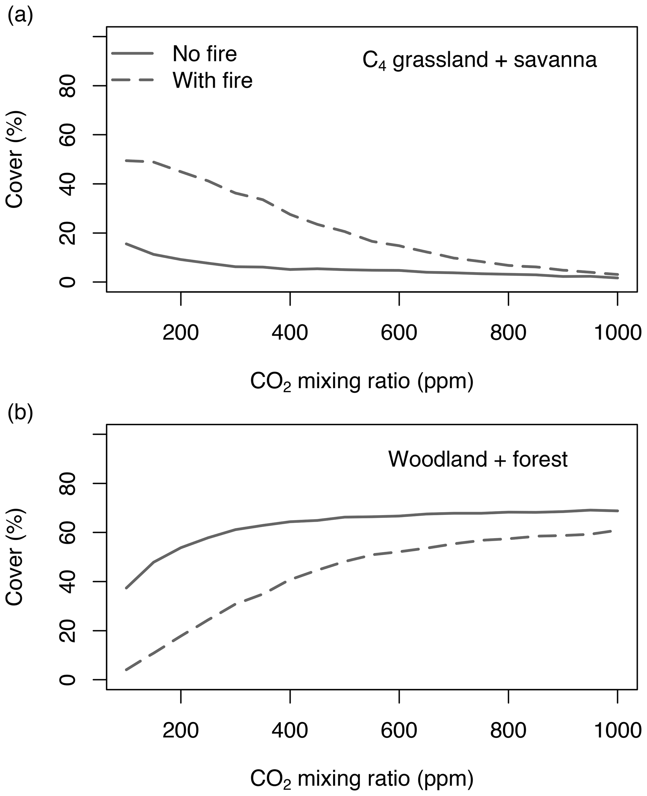
Figure 1Area of Africa covered by (a) C4-dominated (C4 grassland and savanna) and (b) C3-dominated (woodland and forest) vegetation under equilibrium conditions. Simulations were conducted until vegetation reached an equilibrium state under fixed CO2. Differences between simulations without fire (solid lines) and with fire (dashed lines) indicate that both C3- and C4-dominated vegetation states are possible. Figure S1 shows cover fractions separated by biome type.
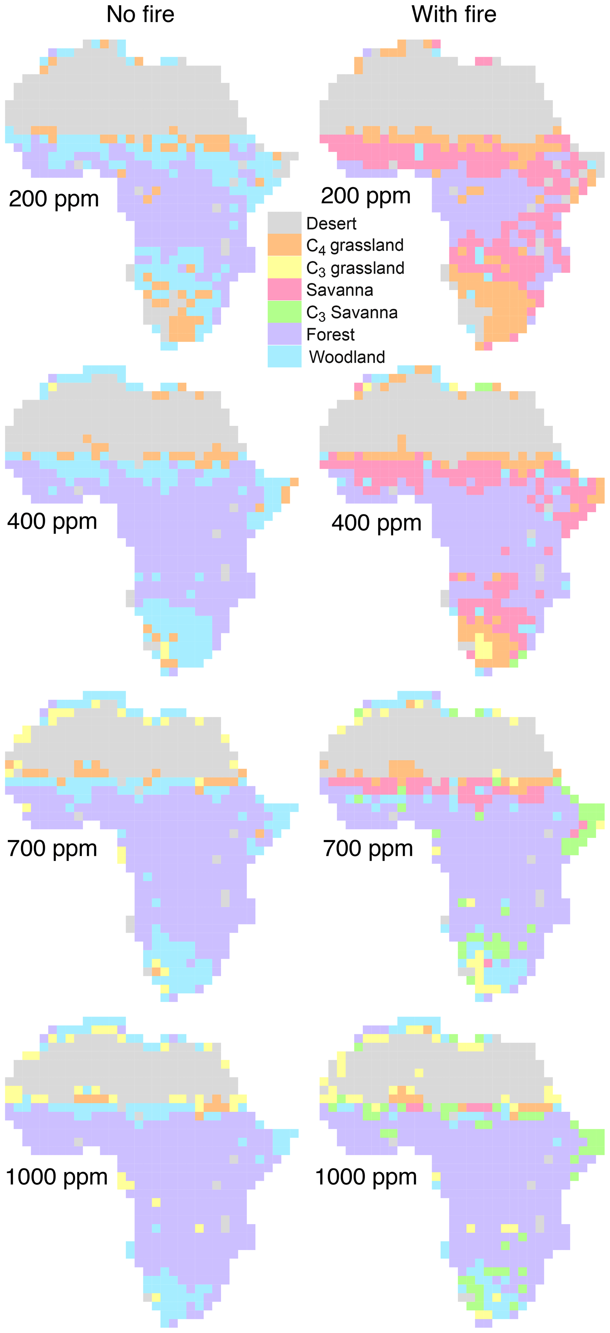
Figure 2Biome distribution at different CO2 mixing ratios and in the presence or absence of fire. Simulations were conducted until vegetation reached an equilibrium state under a constant CO2 mixing ratio.
The time until vegetation reaches an equilibrium state varies substantially in different biomes and for different CO2 mixing ratios. Times are longest in more open ecosystems, that is in grasslands, woodlands and savannas (Fig. 3). In most biomes, times tend to increase with CO2. Times are shortest in forests. The duration is generally longer in the presence of fire than in the absence of fire. When averaged across all biomes and simulations with and without fire, times to reach an equilibrium state increase from approximately 242 years for 200 ppm to 898 years for 1000 ppm.
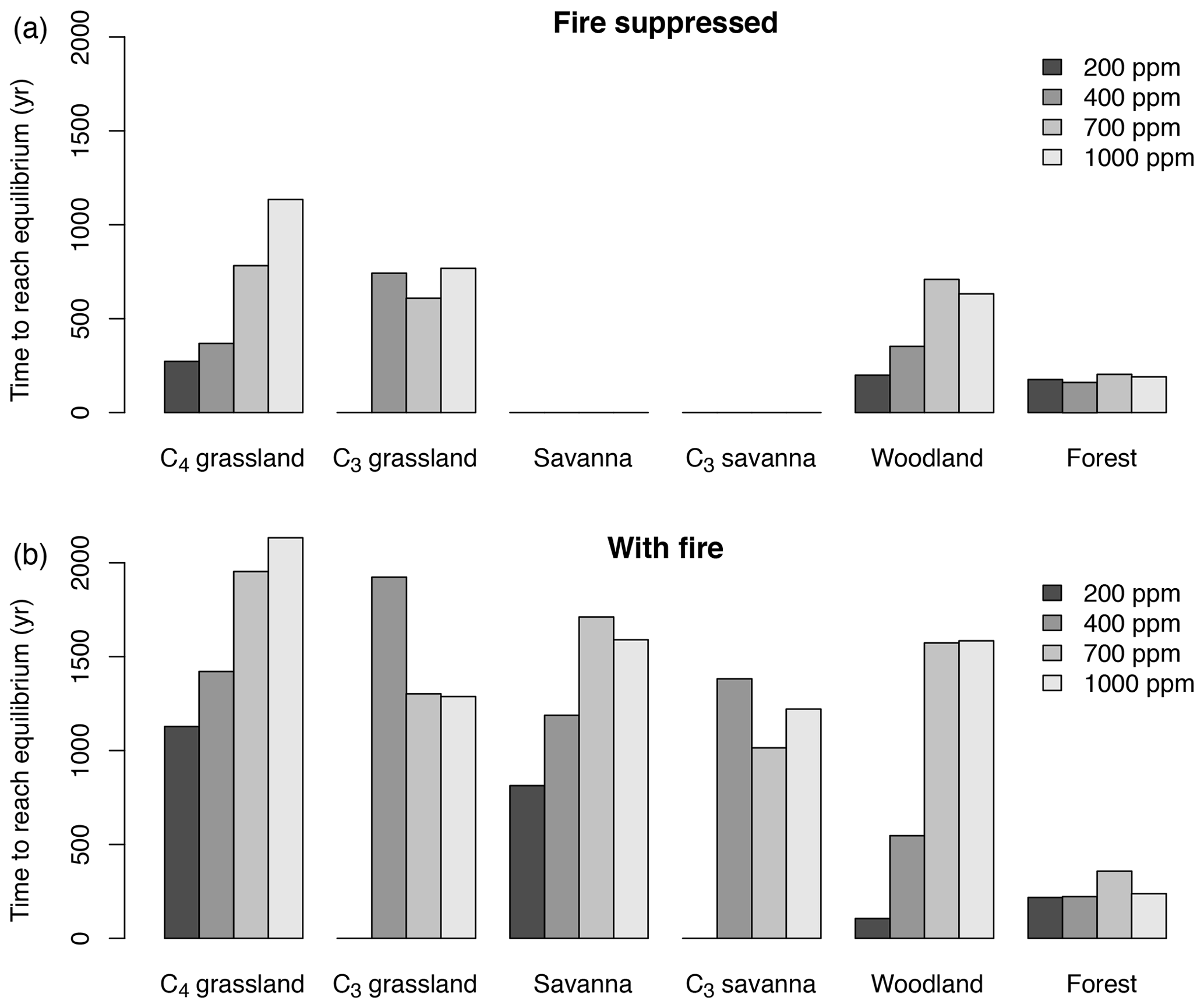
Figure 3Time required to reach the equilibrium biome state in simulations with fixed CO2 mixing ratio. Time was averaged for different biome types and different CO2 mixing ratios. Times to reach equilibrium are shortest in forest and do not respond strongly to CO2. In more open ecosystems (grassland, savanna, woodland) times to reach equilibrium are longer than in forests, and equilibration times increase as CO2 increases. Times to reach equilibrium are shorter under fire suppression (b) than in the presence of fire (a).
3.2 Transient vegetation state and forcing lags
When vegetation is initialized at a CO2 mixing ratio of 100 ppm or 1000 ppm and CO2 increases or decreases progressively in transient simulations, the area covered by different biome types at a given CO2 mixing ratio deviates considerably from the cover in equilibrium simulations (Fig. 4). This pattern is consistent in simulations both with and without fire. Deviance indicates that vegetation is not in equilibrium with the environment and that it lags behind the environmental forcing. At low and increasing CO2, the area covered by grasslands and savanna increases steeply and overshoots the initial cover at 100 ppm, mainly because grasslands invade deserts. As CO2 increases, the areas covered by C3- and C4-dominated vegetation approach the equilibrium state. Trees suppress grasses and eventually fire occurrence, such that forests ultimately manage to invade most of the vegetated area. The deviation between equilibrium and transient cover of C3-dominated vegetation for slow changes of CO2 in the presence of fire (Fig. 4d) is due to transitions from C4 grasslands and savannas to C3 grasslands and C3 savannas.
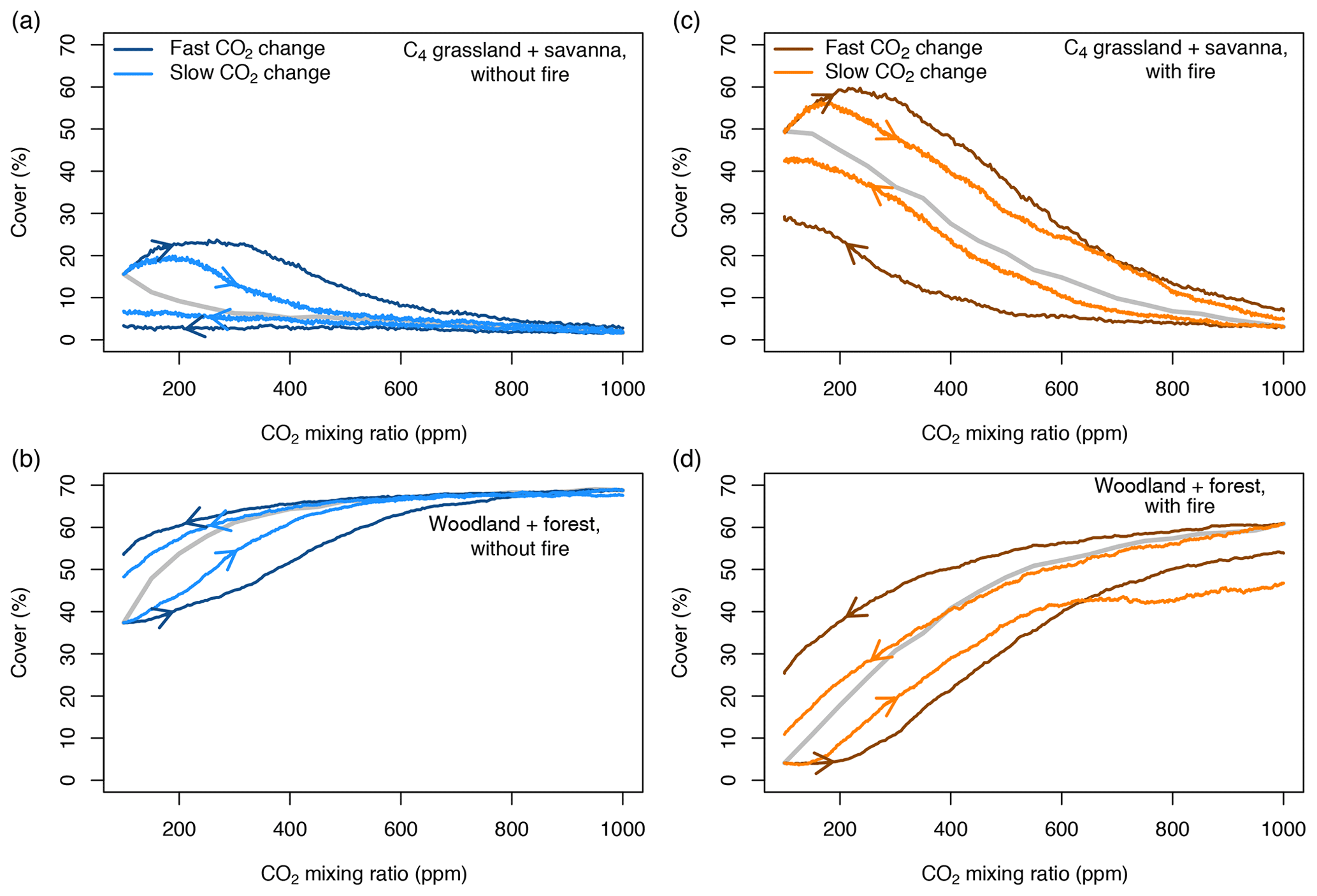
Figure 4Percentages covered by C3- and C4-dominated vegetation in the presence and absence of fire. CO2 is increased or decreased at two different rates between 100 and 1000 ppm. The gray lines indicate vegetation cover in equilibrium simulations (similar to Fig. 1). Arrows indicate whether CO2 increases or decreases.
The aDGVM simulates similar lag effects when CO2 decreases, indicating hysteresis, which is a signature of alternative ecosystem states. The change of vegetation cover in transient simulation runs is nonlinear, although the CO2 forcing changes linearly. In summary, this result confirms our first prediction, i.e., transient vegetation states deviate from the equilibrium state and forcing lags occur.
The rate at which CO2 increases or decreases has a strong impact on the size of the forcing lags (Fig. 4). Fast changes in CO2 imply larger lags than slow changes in CO2. Lags are larger at low and intermediate CO2 mixing ratios and decrease at higher CO2, irrespective of the rate of change of CO2. This result verifies the second prediction.
3.3 Fire and disturbance lags
A comparison of simulations with and without fire shows that fire increases the lag between the CO2 forcing and vegetation (Fig. 4). In the scenario with rapidly changing CO2 mixing ratio, the maximum lag size averaged for all of Africa for C4-dominated biomes is 20 % and 16.3 % with and without fire, respectively, and the maximum lag size for C3-dominated biomes is 19.4 % and 16 % with and without fire, respectively. In scenarios with increasing CO2, lag size is maximized between approximately 200 and 300 ppm. When integrated along the entire CO2 gradient, the mean lag size for C4-dominated biomes is 11.8 % and 6.7 % with and without fire, respectively; the mean lag size for C3-dominated biomes is 11.9 % and 6.4 % with and without fire, respectively. These patterns are similar in simulations with slowly changing CO2 mixing ratio, but percentages are systematically lower. The time to reach equilibrium is longer in simulations with fire than in simulations without fire (Fig. 3), in particular in fire-driven biome types. Times are similar in forests with dense tree canopy, where aDGVM does not simulate fire.
When CO2 is held constant after the transient phase, vegetation converges towards the equilibrium state. In simulations without fire, times to reach equilibrium were similar in equilibrium simulations and in transient simulations with both slow and fast increases or decreases of CO2 (Figs. 5, 6). In simulations with fire, we generally observed longer times than in simulations without fire, particularly in grassland and savanna areas and for decreasing CO2 (Fig. 6). Longer times in the presence of fire can be attributed to hysteresis effects. High fire activity traps vegetation in a fire-driven state and prevents biome transitions into alternative vegetation states. In simulations with decreasing CO2 and fire included, times to reach equilibrium in grasslands and savannas were considerably longer in transient simulations than in equilibrium simulations (Fig. 6). These findings support our third prediction that disturbance lags amplify forcing lags and are particularly relevant in fire-driven systems.
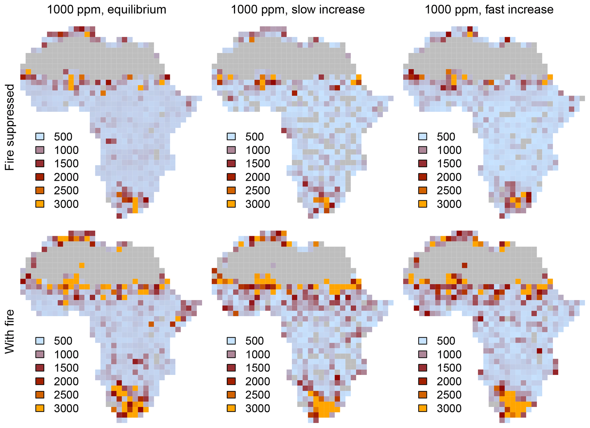
Figure 5Time required to reach equilibrium in equilibrium simulations and transient simulations with both slow and fast increases in CO2. Note that 3000 years in the legend means ≥3000 years, because simulations were run for a maximum of 3000 years.
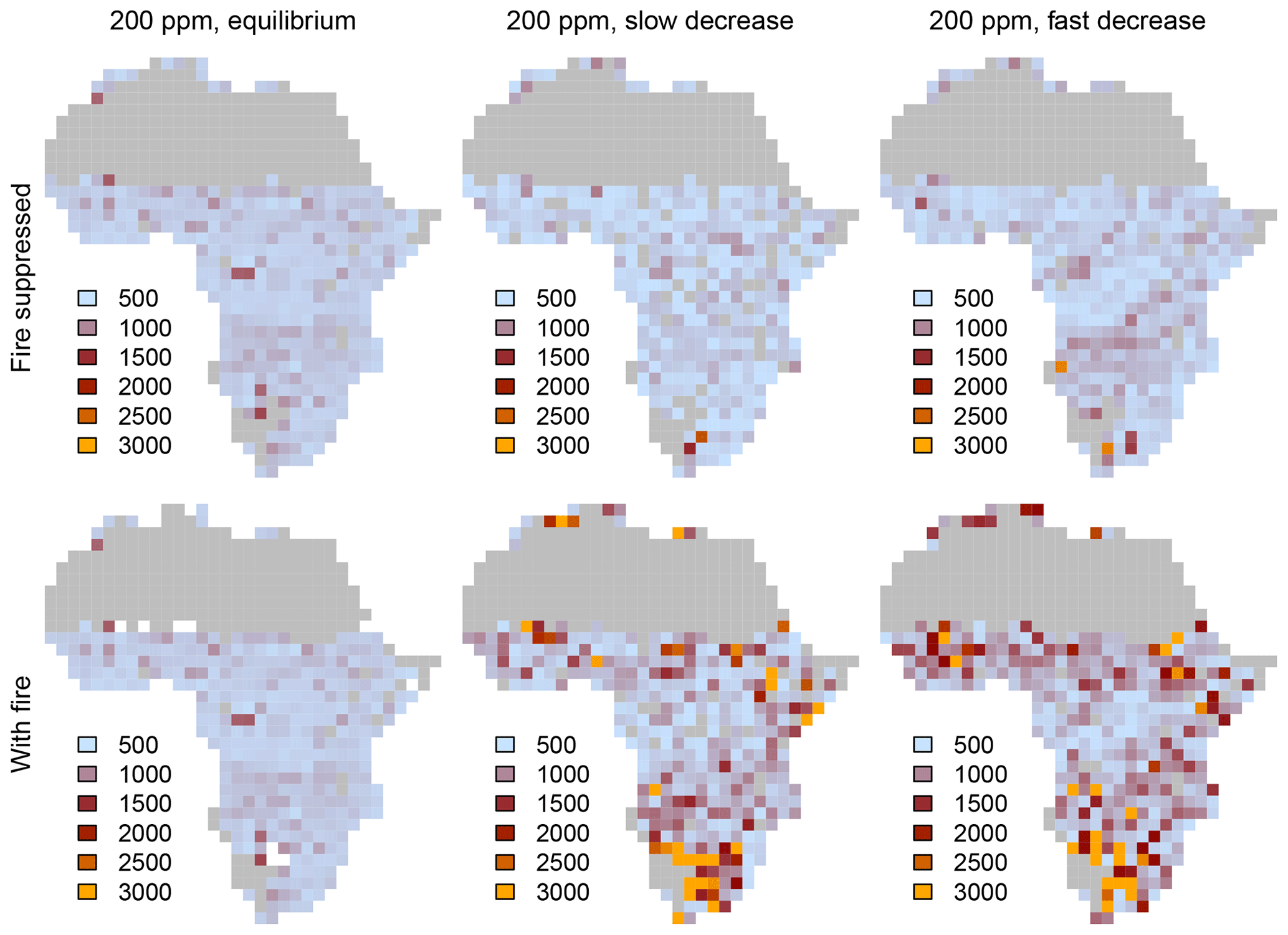
Figure 6Time required to reach equilibrium in equilibrium simulations and transient simulations with both slow and fast decreases in CO2. Note that 3000 years in the legend means ≥3000 years, because simulations were run for a maximum of 3000 years.
3.4 Carbon and tree cover debt
Forcing lags and disturbance lags imply carbon and tree cover debt (for increasing CO2, Fig. 7) or surplus (for decreasing CO2, Fig. S2). Debt means that at a given CO2 mixing ratio, tree cover and carbon stocks are lower in transient simulations than in equilibrium simulations at the same CO2 level. Hence, we define debt as carbon storage potential that has not been realized yet and carbon that the atmosphere owes to vegetation. Accordingly, surplus means that tree cover and carbon are higher in transient simulations than in equilibrium simulations and that vegetation owes carbon to the atmosphere. Where debts and surpluses occur, carbon and tree cover are committed to further changes, even if environmental forcings stabilize, unless tipping-point behavior inhibits vegetation change or allows rapid vegetation changes that compensate for debt or surplus.
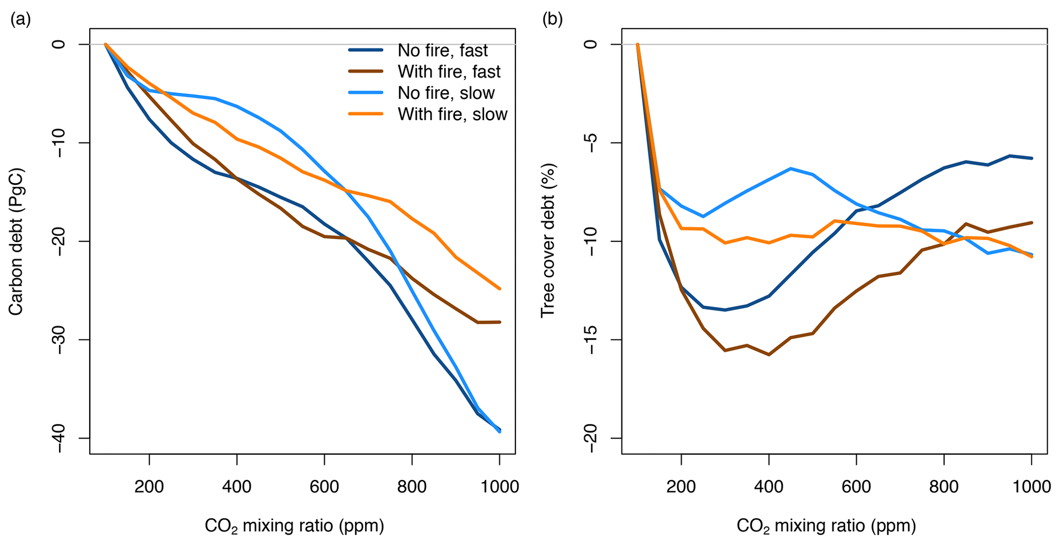
Figure 7Debt of vegetation carbon and tree cover when the atmospheric CO2 mixing ratio increases. Lines represent differences between transient and equilibrium simulations averaged for all study sites in Africa (simulated at 2∘ resolution). See Fig. S2 for decreasing CO2 and associated tree cover and carbon surplus.
Carbon debt increases over the entire CO2 gradient. At current CO2 levels of 400 ppm, carbon debt for Africa is between −6.3 and −13.6 PgC for different scenarios, and it increases to values between −24.8 and −39.9 PgC for 1000 ppm. At high CO2, debt is higher for simulations without fire than for simulations with fire due to the combined effects of forcing and disturbance lags.
Tree cover debt in the presence of fire peaks at values around −15 % between 300 and 400 ppm, i.e., at current CO2 levels. Debt decreases at higher CO2 mixing ratios to values between −5.8 % and −10 %, depending on the scenario. Debt is generally larger in the presence of fire and when CO2 changes rapidly. The maximum deviance between transient and equilibrium state (maximum debt and surplus) varies spatially with higher deviance in savannas and woodlands surrounding the central African forest and in the presence of fire. Tree cover debt saturates or decreases at higher CO2 mixing ratios because tree cover in a grid cell is constrained by canopy closure. At higher CO2 mixing ratios large fractions of Africa reach a forest state and canopy closure. Tree cover debt in these areas is zero. In contrast, biomass in a grid cell and hence biomass debt can further increase even if canopy closure occurs.
3.5 Sensitivity of biome cover to CO2
The sensitivity of the fractional cover of different biome types to changes in CO2 is influenced by the actual values of CO2 (Fig. 8a, b). In equilibrium simulations, the cover of C3-dominated biomes is most sensitive at low CO2 mixing ratios and it decreases as CO2 increases. In simulations with fire, sensitivity of C4-dominated biomes is hump-shaped with a peak at ca. 380 ppm. In transient simulations, both C3- and C4-dominated biomes are most sensitive to changes in CO2 mixing ratios between 200 and 600 ppm, depending on the specific scenario (Fig. 8c, d). Sensitivity is generally higher in the presence of fire than in the absence of fire. For rapidly changing CO2, the peak is found at higher CO2 mixing ratios than for slowly changing CO2. These results support our fourth prediction.

Figure 8Sensitivity of vegetation cover change to changes in the atmospheric CO2 mixing ratio (in percent change of vegetation cover per part per million increase). Upper panels (a, b) show equilibrium simulations; lower panels (c, d) show transient simulations.
3.6 Responses to RCP scenarios
Simulations for CO2 mixing ratios following trajectories of different RCP scenarios indicate carbon debt (Fig. 9a) and tree cover debt (Fig. 9b) as the CO2 mixing ratio increases, similar to the simulations with linear changes of CO2 (Fig. 7). At the current CO2 mixing ratio of approximately 400 ppm, aboveground tree carbon debt is between −8.9 PgC without fire and −16.5 PgC with fire. In the RCP2.6 and 4.5 scenarios, carbon debt in Africa accumulates to peak values between −9.9 and −18 PgC and between −12.9 and −22 PgC, respectively, and then decreases because in these scenarios CO2 decreases (RCP2.6) or saturates (RCP4.5) at the middle of the century. In RCP6.0, debt accumulates to values between −21.2 and −31 PgC; in RCP8.5 it accumulates to values between −47.5 and −60 PgC until 2100. In contrast, tree cover debt peaks between ca. 300 and 350 ppm at values between −3.3 % and −17 % in the presence or absence of fire, respectively. As in the simulations with constant changes in CO2, tree cover debt decreases as the CO2 mixing ratio increases towards the end of the century, with a rate depending on the specific RCP scenario. Generally, both carbon and tree cover debt are higher in the presence of fire than under fire suppression.
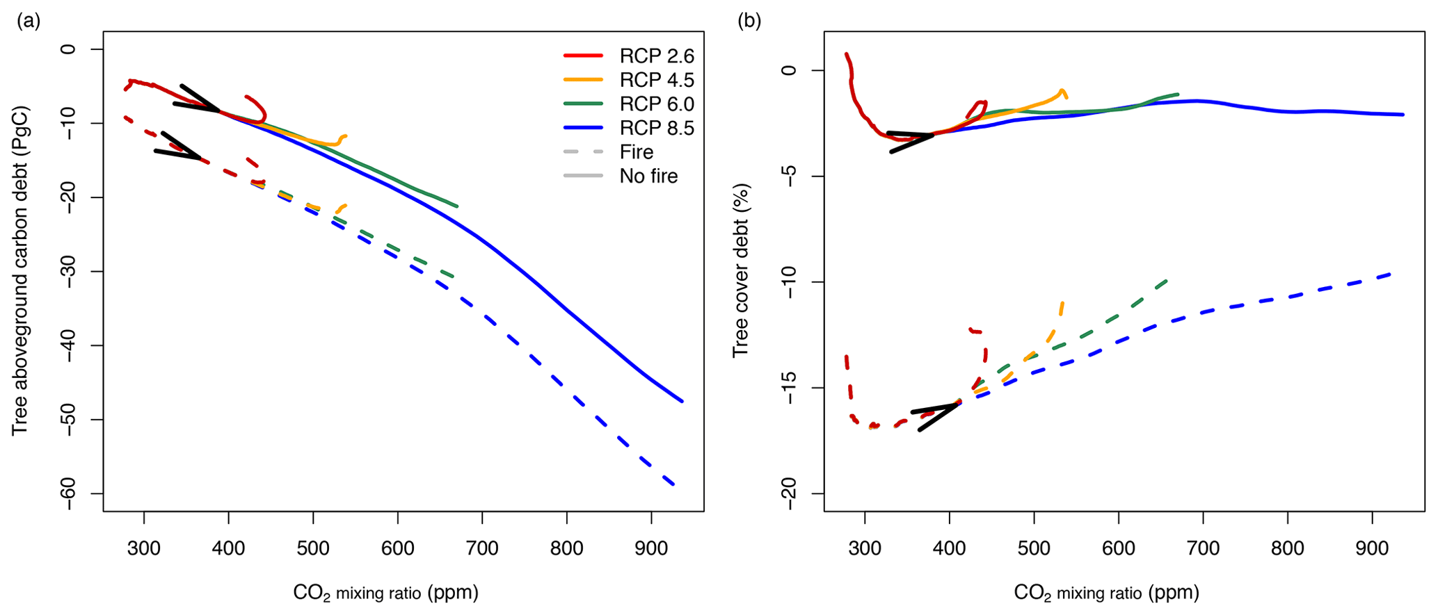
Figure 9Vegetation carbon and tree cover debt when the atmospheric CO2 mixing ratio increases according to different RCP scenarios. Lines represent differences between transient and equilibrium simulations averaged for all study sites in Africa (simulated at 2∘ resolution). Solid lines represent simulations without fire, and dashed lines represent simulations with fire. Arrows indicate time between 1950 and 2100.
Using a dynamic vegetation model, we predict that vegetation exposed to transient environmental forcing is not in equilibrium with environmental conditions and that such transient vegetation states deviate from the vegetation state expected for the prevailing environmental conditions. Vegetation development lags behind changing environmental drivers due to forcing lags. The size of the forcing lag depends both on actual environmental conditions and on the rate at which conditions change. Disturbance lags caused by fire can amplify forcing lags in areas where multiple vegetation states are possible such as savanna areas that also support forest. Our results indicate that vegetation in Africa is most sensitive to changes in the atmospheric CO2 mixing ratio at current conditions. Hence, even if anthropogenic emissions of CO2 and the accumulation of CO2 in the atmosphere were to level off in the near future, ecosystems will still be committed to considerable changes.
Our model simulations are consistent with previous aDGVM model results indicating that biome distributions over large areas of Africa are dependent on fire (Higgins and Scheiter, 2012) and that these distributions are contingent on historic vegetation states and likely to change under elevated CO2 (Scheiter and Higgins, 2009; Higgins and Scheiter, 2012; Moncrieff et al., 2014). While we only considered transient vegetation dynamics in previous aDGVM studies, we now show that these results also hold true for simulations with equilibrium conditions. In our transient simulations we further show that linear forcing in CO2 can cause nonlinear responses in vegetation states. This result indicates internal feedback loops and tipping-point behavior in the climate–fire–vegetation system (Scheffer et al., 2001) and supports our previous findings (Higgins and Scheiter, 2012). The potential for alternate biomes, dependent on fire, and hysteresis effects occurs both in equilibrium simulations with fixed CO2 and in transient simulations with a variable CO2 mixing ratio. These effects occur over the entire CO2 gradient between 100 and 1000 ppm.
4.1 Understanding forcing, disturbance and successional lags
Lags between environmental conditions and vegetation states occur if environmental conditions change faster than vegetation can respond. In such a situation, transient vegetation states deviate from the vegetation states that one would expect if prevailing environmental conditions remained constant for a sufficiently long duration. The lag size is defined by the integrated effect of interacting processes including delayed responses in ecophysiology, demography, migration and succession and by the different timescales on which these processes operate (Peñuelas et al., 2013). Rates of change in environmental forcing and intensity and frequency of disturbances further influence lag size. In aDGVM simulations we find a sequence of vegetation responses to changes in the CO2 mixing ratio that operate at different temporal scales. When CO2 increases, leaf-level photosynthesis and respiration increase instantaneously following the ecophysiology models implemented in aDGVM (Farquhar et al., 1980; Collatz et al., 1991, 1992, Fig. 10). These adaptations imply higher carbon gain, water use efficiency and growth of individual trees in the growing season as well as higher reproduction rates, because in aDGVM the amount of carbon allocated to reproduction is a function of peak carbon gain. Free-air carbon enrichment (FACE) experiments and open top chamber experiments for elevated CO2 indicate similar responses at the leaf level (e.g., Hickler et al., 2015; Kgope et al., 2010, Raubenheimer, Ripley, et al., unpublished).
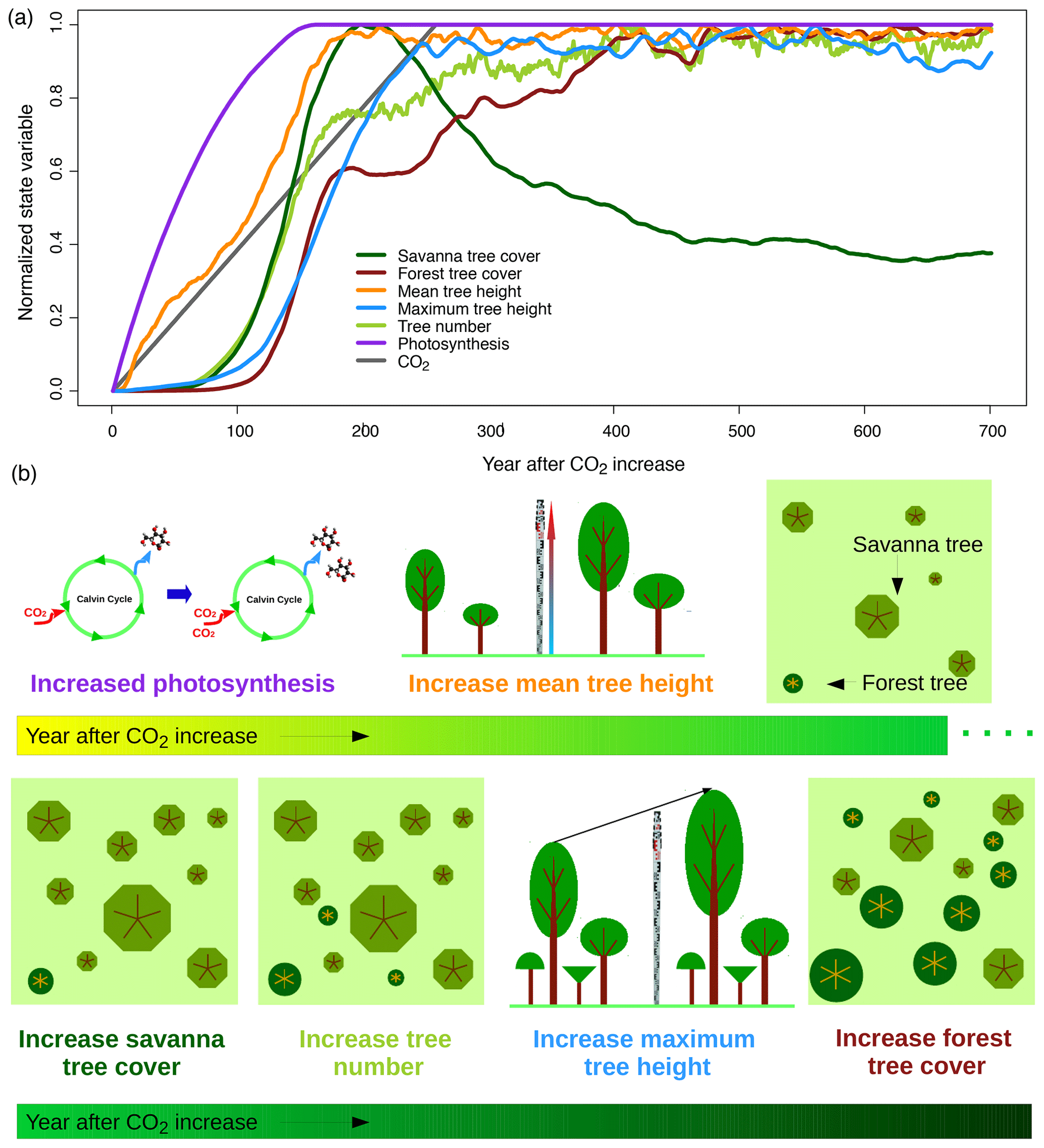
Figure 10Vegetation responses to increasing CO2. Panels show (a) time series of different state variables at a savanna study site in South Africa (26∘ S, 28∘ E) and (b) a schematic illustration of processes. State variables represent averages of 200 replicate simulation runs for the site. Normalization of state variables between zero and 1 based on minimum and maximum values was applied to be able to illustrate temporal lags between variables. Figure S3 provides the time series without normalization and with units of respective variables.
In aDGVM, higher growth and reproduction rates of individual plants modify plant population dynamics and vegetation structure. The model simulates an increase in mean tree height after CO2 starts increasing (Fig. 10). After a delay of approximately 70 years, trees can establish more successfully and tree number and savanna tree cover increase. Tree cover increases can be attributed to increases both in tree height, which in aDGVM is linked to an increase in a tree's crown area, and in tree number. Increases in maximum tree height lag behind mean tree height and tree numbers (Fig. 10). All population-level responses in the model are slower than leaf-level responses and lag behind ecophysiological adaptations.
Observing population-level responses to elevated CO2 in reality is challenging. Historic data from field surveys (Stevens et al., 2017; O'Connor et al., 2014) and remote sensing (Donohue et al., 2013; Skowno et al., 2017) indicate woody encroachment in many savanna areas. These changes were often attributed to historic increases in CO2 (Midgley and Bond, 2015) but also to land use activities such as overgrazing (Roques et al., 2001). Yet, the strength of CO2 fertilization effects is debated (Körner et al., 2005) and free-air carbon enrichment (FACE) experiments indicate complex responses of vegetation to elevated CO2 at the population level (Hickler et al., 2015). Nutrient limitations (Hickler et al., 2015) and effects of mycorrhizal associations on nutrient economy (Terrer et al., 2016) may add to the complexity of these responses. FACE experiments in savannas and subtropical ecosystems are rare. An exception is OzFACE in Queensland, Australia (Stokes et al., 2005), which found increased growth rates for Eucalyptus and Acacia species. Previous studies showed that CO2 fertilization effects are strong in aDGVM and that the strong CO2 effects can compensate for other predicted changes in climate drivers, such as reduced rainfall (Scheiter et al., 2015). If aDGVM overestimates the strength of CO2 fertilization effects and the sensitivity of vegetation to elevated CO2, the size of carbon debt due to lag effects may be overestimated, while the lag size may be underestimated. We are however confident that even with reduced CO2 sensitivity the overall response pattern would remain, although the quantities might change. In Scheiter et al. (2018) we show that simulated woody cover increases in the Limpopo Province, South Africa, and under current conditions broadly agrees with remote sensing observations from Stevens et al. (2017), indicating that aDGVM simulates plausible responses to climate change for historic and current conditions.
Disturbance lags in fire-driven savannas are created by a well-known feedback mechanism between fire and vegetation (Higgins and Scheiter, 2012; Hoffmann et al., 2012). Regular fire is a demographic bottleneck for tree establishment and traps trees in a juvenile state (Higgins et al., 2000). At the population scale, fire preserves a characteristic, open-savanna vegetation state (Scheiter and Higgins, 2009) and keeps vegetation from reaching an equilibrium vegetation state, typically woodland or forest with higher tree cover, expected under the prevailing environmental conditions. Yet, reduced fire activity (Hoffmann et al., 2012) or increased tree growth rates due to CO2 fertilization (Bond and Midgley, 2000) allow more trees to escape the fire trap due to increased growth rates. As a consequence, the increasing tree cover starts to exclude grasses and curtails fire frequency due to reduced fine fuel loads. This dynamic feedback between vegetation and fire dynamics implies that rapid transitions between savanna and forest states are possible.
Once fire is excluded at high CO2 mixing ratios, successional lags delay the establishment of an equilibrium state. These lags are a direct consequence of disturbances and they emerge if plant community composition in the equilibrium state deviates from transient, post-disturbance community composition. The aDGVM simulates fire-tolerant but shade-intolerant savanna trees and fire-intolerant but shade-tolerant forest trees (Scheiter et al., 2012). At low CO2 and intermediate rainfall, aDGVM simulates a fire-driven savanna state with predominantly savanna trees. Reduced fire activity and transitions to woody-plant-dominated habitats imply that savanna trees and grasses are outcompeted and gradually replaced by forest trees (Fig. 10). Successional dynamics are slow and delay the adaptation of community composition to elevated CO2. Empirical studies support successional lags in communities (Fauset et al., 2012; Esquivel-Muelbert et al., 2019), although these studies reported community responses to drought rather than CO2.
We found that fire-driven savanna and grassland ecosystems take longer to reach equilibrium after the CO2 forcing stabilizes than forests. Forests are faster to stabilize and to balance their carbon and tree cover debt. In our simulations, this behavior is driven by disturbance-related lags caused by fire. Fire generates a dynamic disequilibrium between climate and vegetation, and it prevents both savanna and forest trees from recruiting, from transitioning into the adult state and from developing a closed canopy. When tree cover exceeds a critical threshold, fire is suppressed and rapid canopy closure is possible. Fire rarely occurs in simulated forests, and therefore they reach equilibrium faster than other biome types. Fire activity in forests is, however, sufficient to slightly increase times to reach equilibrium when compared to simulations with fire suppressed. Moreover, forests represent the final stage in succession in ecosystems simulated by aDGVM. Hence, forests do not allow for further succession in contrast to grasslands and savannas, where savanna trees can invade grasslands and be replaced by forest trees in later successional stages. The aDGVM might underestimate lags in forest systems in contrast to alternative DGVMs or forest models that simulate a higher number of plant functional types (PFTs) or species (e.g., Hickler et al., 2012) or that allow plant traits and community composition within a forest system to adapt to changing environmental drivers (Scheiter et al., 2013).
4.2 Implications for adaptation, mitigation and policy
Lags between transient and equilibrium coverage of different vegetation types or biome types imply debt or surplus in tree cover (Jones et al., 2009), carbon storage, biogeochemical fluxes and community composition (Bertrand et al., 2016). These lags commit ecosystems to further changes even if the rate of climate change is reduced and the climate system converges towards an equilibrium state (Jones et al., 2009; Port et al., 2012; Pugh et al., 2018). This finding has important implications for the development of adaptation and mitigation strategies for climate change.
First, it indicates that such strategies cannot be developed purely based on observed contemporary transient states when attempting to mitigate further changing of climatic drivers. There is an urgent need to understand equilibrium vegetation states and committed changes in vegetation states and to take them into account in management policies (Svenning and Sandel, 2013). Lag effects are also central to understanding resilience of an ecosystem (Holling, 1973; Walker et al., 2004).
Second, our findings imply a high priority and potential for managing fire-dependent ecosystems such as savannas. It has been argued that in these ecosystems, elevated CO2 is the main driver for shrub encroachment and transitions to forest (Higgins and Scheiter, 2012; Midgley and Bond, 2015). Suitable management intervention can oppose CO2 fertilization effects and delay undesired vegetation changes (Scheiter and Savadogo, 2016). For instance, the introduction of fire can increase lags between transient and equilibrium vegetation states, whereas fire suppression for example by grazing (Pfeiffer et al., 2019) or fire management (Scheiter et al., 2015) can reduce disturbance-related lags. Other disturbances or land use activities such as herbivory or fuelwood harvesting have similar effects (Scheiter and Savadogo, 2016). Hence the potential for these ecosystems to persist in a disequilibrium state relative to climate and CO2 creates the opportunity to mitigate changes brought about by global change through management interventions. Conversely, allowing these systems to reach their equilibrium state has the potential to increase the global land carbon sink. While such management is relevant for carbon sequestration (Bastin et al., 2019), it is likely to lead to loss of biodiversity concomitant with losses of open-savanna and grassland ecosystems (Veldman et al., 2015; Bond et al., 2019). Given the increasing lag size between transient and equilibrium vegetation states, management should decide at the local scale if current or desired vegetation states should be maintained as long as possible or if ecosystems should be managed to account for vegetation changes expected in the near future. Ignoring committed changes might imply rapid vegetation shifts that inhibit sustainable management actions.
Third, we found that the rate at which environmental conditions change determines the size of the lag between transient and equilibrium vegetation. Following the RCP8.5 trajectory instead of the RCP2.6 trajectory will therefore increase carbon debt due to both higher CO2 mixing ratio and the acceleration of CO2 enrichment in the atmosphere. If emissions follow the RCP2.6 scenario and stabilize after 2100, then ecosystems in Africa would continue to absorb 9 PgC or 18 PgC from the atmosphere in the presence or absence of fire until they reach an equilibrium state with environmental conditions. In contrast, ecosystems would absorb 47.5 PgC or 60 PgC in the presence or absence of fire in the RCP8.5 scenario.
Finally, climate and greenhouse gas concentrations in the atmosphere are likely to change at an unprecedented rate (Prentice et al., 1993; Foster et al., 2017). Our results indicate that vegetation is most sensitive to changes in atmospheric CO2 at the currently prevailing levels and values expected in the near future (between approximately 350 and 500 ppm, depending on the simulation scenario and response variable investigated). Hence, we are currently in a period when small changes in CO2 are likely to have large impacts on long-term vegetation change. The results also show that restoring savannas from heavily encroached wood-dominated states is a long process, particularly if fire is lost from these ecosystems. This finding raises the urgent need for society to act and reduce greenhouse gas emissions as the window of opportunity where human intervention can contribute to reversing climate change impacts might close soon.
4.3 Implications for vegetation modeling
The lag effects identified in our study have important implications for vegetation modeling and the process of testing and benchmarking models. Lag effects are prevalent both in results from transient model simulations using time series of climate data and in data used for benchmarking, including remote sensing products (Saatchi et al., 2011; Simard et al., 2011; Avitabile et al., 2016) or data collected in field surveys. Previous studies identified sources of uncertainty in data–model comparisons (Scheiter and Higgins, 2009; Langan et al., 2017) related to model uncertainties or data uncertainties. We argue that the presence of forcing and disturbance lags can add to disagreement between benchmarks and simulation results, such as modeled and satellite-derived productivity (Smith et al., 2016), carbon stocks, vegetation type, or species composition. Although DGVMs typically simulate transient vegetation states based on time series obtained from climate models, we argue that to improve the benchmarking process, we need to ensure that data and models represent similar successional stages. This can be achieved, e.g., by applying appropriate model initialization methods using historical climate data, land use and fire history or by considering effects of historic legacies on vegetation (Moncrieff et al., 2014). For example, Rödig et al. (2017) used the Simard et al. (2011) vegetation height product to ensure that successional stages simulated with the FORMIND model agree with observed successional stages. We concede that this is not an easy task as large-scale data on equilibrium vegetation states or lag sizes are typically not available, and as vegetation states have been modified by human land use for millennia. Remote sensing products such as the GEDI mission (gedi.umd.edu) may provide high-resolution data required to initialize models with biomass and vegetation structure.
The emergence of lag effects also highlights the relevance of adequate representation of demography, succession and disturbance regimes in vegetation models and makes a case for cohort- or individual-based approaches. Understanding and quantifying lags necessitates prioritization and further model development with respect to these processes (Fisher et al., 2018) as well as improved knowledge of the rates at which these processes operate. Accurate representation of rates of changes may contribute to improve data–model agreement (Smith et al., 2016). In-depth model testing against available long-term observations of successional changes in response to climate change and disturbance can further reduce model uncertainties. Fire or herbivore manipulation experiments conducted in Kruger National Park (Higgins et al., 2007) or in Burkina Faso (Savadogo et al., 2009) exemplify such datasets, in particular because they not only provide time series for benchmarking but also include relevant and documented disturbance processes under controlled conditions.
In this study, we only considered natural fire regimes as simulated by aDGVM. However, to understand the full complexity of vegetation lags, further disturbances need to be taken into consideration. This includes anthropogenic fire (planned management fires as well as accidental fires), but also herbivory (grazing and browsing), fuelwood harvesting, deforestation, and conversion of natural land to agricultural or forestry areas. In this study we only quantified lags in biome shifts, tree cover and aboveground carbon storage, but our framework can be extended to further ecosystem services in follow-up studies. In addition, we only considered changes in CO2 in this study whereas changes in other key variables influencing vegetation, particularly precipitation and temperature, were ignored. Previous aDGVM studies show that change in CO2 is the main driver of simulated future vegetation change due to strong CO2 fertilization effects (Scheiter and Higgins, 2009; Scheiter et al., 2015; Scheiter et al., 2018; Martens et al., unpublished). We therefore expect that using time series of both CO2 and climatic drivers following RCP scenarios will not change the fundamental results of our study. This expectation is supported by simulation results using various climatic drivers for RCP8.5 and 4.5 (Pfeiffer et al., unpublished).
4.4 Further lags in the climate–vegetation system
In this study, we identified three lags between transient and equilibrium vegetation, namely forcing, disturbance and successional lags. Yet, due to the design of aDGVM our study ignores other lag effects in the climate–vegetation system.
Migration lags occur due to a limited speed of seed dispersal and migration under variable climate. Dispersal and migration can, particularly in vegetation, typically not keep pace with climate change (Loarie et al., 2009). Migration lags have been investigated, but often using statistical approaches such as species distribution modeling (Thuiller et al., 2005). Extending DGVMs or forest models with dispersal models is, however, possible. For instance, Blanco et al. (2014) used a spatially explicit version of aDGVM to show that forest expansion rates in Araucaria forest–grassland mosaics in southern Brazil are sensitive to characteristics of the dispersal traits of Araucaria trees. Sato and Ise (2012) showed with SEIB-DGVM that including dispersal in projections of African vegetation until 2100 implies lagged responses in simulated biome boundary shifts. Nabel et al. (2013) used the TreeMig model to illustrate the complexity of simulating seed dispersal and migration in heterogeneous and variable environments.
Once a species has migrated into another suitable region, establishment lags due to competition between established and invading species can occur and prevent establishment of invading species. To quantify establishment lags in DGVMs, an accurate description of competition, demography and succession is necessary. Scheiter et al. (2013) argued that competition is often not adequately described in DGVMs. More advanced models are required that simulate competitive interactions between individual plants for space, light, nutrients and water and consider allelopathic interactions. Novel approaches based on trait variation such as aDGVM2 (Scheiter et al., 2013; Langan et al., 2017), JeDi-DGVM (Pavlick et al., 2013) or LPJmL-FIT (Sakschewski et al., 2015) can be applied to identify establishment lags based on their detailed description of individual plants and plant communities that are characterized by variable and dynamic traits instead of relying on a fixed number of static plant functional types.
At longer timescales, evolutionary lags occur due to evolution of species adapted to changing environmental conditions or to disturbance regimes (e.g., Simon et al., 2009; Guerrero et al., 2013). More advanced vegetation models are required to simulate how evolutionary processes such as trait inheritance, mutation and crossover allow plants to adapt to changing environmental conditions over many generations. While aDGVM2 (Scheiter et al., 2013) includes these mechanisms, the model has so far not been applied in an evolutionary context. Such an application would require a re-parametrization of mutation and crossover rates using empirical data to account for the temporal component of evolutionary processes.
Finally, atmosphere–biosphere lags can occur where delayed responses of vegetation change to environmental change feed back to delay responses of the environment. For example, increasing forest cover due to CO2 fertilization and resulting increase in carbon sequestration may reduce CO2 enrichment in the atmosphere and associated amplification of radiative forcing. Investigation of atmosphere–biosphere lags requires fully coupled models that simulate biogeochemical fluxes between atmosphere and biosphere. Jones et al. (2009) used such a fully coupled model to investigate lags in Amazon forest dieback, but feedbacks to the climate system were not explicitly considered. Port et al. (2012) used the fully coupled MPI ESM to show that lagged responses of vegetation may, in a scenario where CO2 emissions are zero after 2120, reduce atmospheric CO2 by approximately 40 ppm until 2300. Another well-studied example is the Sahel greening phenomenon where smooth changes in rainfall regimes trigger abrupt and delayed responses in vegetation cover due to vegetation–atmosphere feedbacks (Brovkin et al., 1998; Claussen et al., 1999; Foley et al., 2003).
To conclude, our study indicates that vegetation generally lags behind changing atmospheric CO2 mixing ratios. We are currently in a phase of high carbon storage and tree cover debt, and vegetation cover deviates substantially from the committed vegetation state. Our study predicts that vegetation is most sensitive to changes in atmospheric CO2 at current levels of atmospheric CO2 and those expected in the near future. This finding indicates the need to act and reduce greenhouse gas emissions. Lags are larger in fire-dependent systems such as savannas than in arid grasslands or forests. Lag effects in vegetation status need to be considered for the development of management plans or mitigation strategies because we expect further changes in vegetation even if emissions of CO2 and other greenhouse gasses are reduced and the climate system stabilizes. There is an urgent need to understand lag effects in response to not only variable CO2 but also to other key variables of the climate system such as temperature and precipitation, as well as to extreme events such as heat waves or drought.
The aDGVM code as well as scripts to conduct the model experiments and analyze the results are available upon request. Please contact any of the authors.
The supplement related to this article is available online at: https://doi.org/10.5194/bg-17-1147-2020-supplement.
SS, SIH and GRM conceived the study; SS conducted simulations and analyzed results; SS and MP created the figures; and SS led the writing with contributions from all co-authors.
The authors declare that they have no conflict of interest.
This research has been supported by the Deutsche Forschungsgemeinschaft (grant no. SCHE 1719/2-1) and the Bundesministerium für Bildung und Forschung (grant no. 01LL1802B).
The publication of this article was funded by the
Open Access Fund of the Leibniz Association.
This paper was edited by Sönke Zaehle and reviewed by two anonymous referees.
Anderegg, W. R. L., Schwalm, C., Biondi, F., Camarero, J. J., Koch, G., Litvak, M., Ogle, K., Shaw, J. D., Shevliakova, E., Williams, A. P., Wolf, A., Ziaco, E., and Pacala, S.: Pervasive drought legacies in forest ecosystems and their implications for carbon cycle models, Science, 349, 528–532, https://doi.org/10.1126/science.aab1833, 2015. a
Avitabile, V., Herold, M., Heuvelink, G. B. M., Lewis, S. L., Phillips, O. L., Asner, G. P., Armston, J., Ashton, P. S., Banin, L., Bayol, N., Berry, N. J., Boeckx, P., de Jong, B. H. J., DeVries, B., Girardin, C. A. J., Kearsley, E., Lindsell, J. A., Lopez-Gonzalez, G., Lucas, R., Malhi, Y., Morel, A., Mitchard, E. T. A., Nagy, L., Qie, L., Quinones, M. J., Ryan, C. M., Ferry, S. J. W., Sunderland, T., Laurin, G. V., Gatti, R. C., Valentini, R., Verbeeck, H., Wijaya, A., and Willcock, S.: An integrated pan-tropical biomass map using multiple reference datasets, Glob. Change Biol., 22, 1406–1420, https://doi.org/10.1111/gcb.13139, 2016. a
Barnola, J. M., Raynaud, D., Korotkevich, Y. S., and Lorius, C.: Vostok ice core provides 160,000-year record of atmospheric CO2, Nature, 329, 408–414, https://doi.org/10.1038/329408a0, 1987. a
Bastin, J.-F., Finegold, Y., Garcia, C., Mollicone, D., Rezende, M., Routh, D., Zohner, C. M., and Crowther, T. W.: The global tree restoration potential, Science, 365, 76–79, https://doi.org/10.1126/science.aax0848, 2019. a
Beerling, D. J. and Royer, D. L.: Convergent Cenozoic CO2 history, Nat. Geosci., 4, 418–420, https://doi.org/10.1038/ngeo1186, 2011. a, b, c
Bertrand, R., Lenoir, J., Piedallu, C., Riofrio-Dillon, G., de Ruffray, P., Vidal, C., Pierrat, J.-C., and Gegout, J.-C.: Changes in plant community composition lag behind climate warming in lowland forests, Nature, 479, 517–520, 2011. a
Bertrand, R., Riofrio-Dillon, G., Lenoir, J., Drapier, J., de Ruffray, P., Gegout, J.-C., and Loreau, M.: Ecological constraints increase the climatic debt in forests, Nat. Commun., 7, 12643, https://doi.org/10.1038/ncomms12643, 2016. a, b, c, d
Blanco, C. C., Scheiter, S., Sosinski, E., Fidelis, A., Anand, M., and Pillar, V. D.: Feedbacks between vegetation and disturbance processes promote long-term persistence of forest–grassland mosaics in south Brazil, Ecol. Model., 291, 224–232, https://doi.org/10.1016/j.ecolmodel.2014.07.024, 2014. a
Bond, W. J. and Midgley, G. F.: A proposed CO2-controlled mechanism of woody plant invasion in grasslands and savannas, Glob. Change Biol., 6, 865–869, 2000. a
Bond, W. J. and Midgley, J. J.: Ecology of sprouting in woody plants: the persistence niche, Trend. Ecol. Evol., 16, 45–51, 2001. a, b
Bond, W. J., Stevens, N., Midgley, G. F., and Lehmann, C. E. R.: The Trouble with Trees: Afforestation Plans for Africa, Trend. Ecol. Evol., 34, 963–965, https://doi.org/10.1016/j.tree.2019.08.003, 2019. a
Brovkin, V., Claussen, M., Petoukhov, V., and Ganopolski, A.: On the stability of the atmosphere-vegetation system in the Sahara/Sahel region, J. Geophys. Res.-Atmos., 103, 31613–31624, 1998. a
Buitenwerf, R., Bond, W. J., Stevens, N., and Trollope, W. S. W.: Increased tree densities in South African savannas: >50 years of data suggests CO2 as a driver, Glob. Change Biol., 18, 675–684, https://doi.org/10.1111/j.1365-2486.2011.02561.x, 2012. a
Claussen, M., Kubatzki, C., Brovkin, V., Ganopolski, A., Hoelzmann, P., and Pachur, H. J.: Simulation of an abrupt change in Saharan vegetation in the mid-Holocene, Geophys. Res. Lett., 26, 2037–2040, 1999. a
Collatz, G. J., Ball, J. T., Grivet, C., and Berry, J. A.: Physiological and environmental regulation of stomatal conductance, photosynthesis and transpiration: a model that includes a laminar boundary layer, Agr. Forest Meteorol., 54, 107–136, 1991. a
Collatz, G. J., Ribas-Carbo, M., and Berry, J. A.: Coupled photosynthesis-stomatal conductance model for leaves of C4 plants, Austr. J. Plant Physiol., 19, 519–538, 1992. a
Davis, M. B.: Climatic Instability, Time, Lags, and Community Disequilibrium, in: Community Ecology, edited by: Diamond, J. M. and Case, T. J., New York, Harper and Row, 269–284, 1984. a
Davis, M. B. and Botkin, D. B.: Sensitivity of cool-temperate forests and their fossil pollen record to rapid temperature change, Quaternary Res., 23, 327–340, 1985. a, b
Devictor, V., van Swaay, C., Brereton, T., Brotons, L., Chamberlain, D., Heliola, J., Herrando, S., Julliard, R., Kuussaari, M., Lindstrom, A., Reif, J., Roy, D. B., Schweiger, O., Settele, J., Stefanescu, C., Van Strien, A., Van Turnhout, C., Vermouzek, Z., WallisDeVries, M., Wynhoff, I., and Jiguet, F.: Differences in the climatic debts of birds and butterflies at a continental scale, Nat. Clim. Change, 2, 121–124, https://doi.org/10.1038/NCLIMATE1347, 2012. a
Donohue, R. J., Roderick, M. L., R., M. T., and Farquhar, G. D.: Impact of CO2 fertilization on maximum foliage cover across the globe's warm, arid environments, Geophys. Res. Lett., 40, 1–5, https://doi.org/10.1002/grl.50563, 2013. a, b
Esquivel-Muelbert, A., Baker, T. R., Dexter, K. G., Lewis, S. L., Brienen, R. J. W., Feldpausch, T. R., Lloyd, J., Monteagudo-Mendoza, A., Arroyo, L., Alvarez-Davila, E., Higuchi, N., Marimon, B. S., Marimon-Junior, B. H., Silveira, M., Vilanova, E., Gloor, E., Malhi, Y., Chave, J., Barlow, J., Bonal, D., Davila Cardozo, N., Erwin, T., Fauset, S., Herault, B., Laurance, S., Poorter, L., Qie, L., Stahl, C., Sullivan, M. J. P., ter Steege, H., Vos, V. A., Zuidema, P. A., Almeida, E., Almeida de Oliveira, E., Andrade, A., Vieira, S. A., Aragao, L., Araujo-Murakami, A., Arets, E., Aymard C, G. A., Baraloto, C., Camargo, P. B., Barroso, J. G., Bongers, F., Boot, R., Camargo, J. L., Castro, W., Chama Moscoso, V., Comiskey, J., Cornejo Valverde, F., Lola da Costa, A. C., del Aguila Pasquel, J., Di Fiore, A., Fernanda Duque, L., Elias, F., Engel, J., Flores Llampazo, G., Galbraith, D., Herrera Fernandez, R., Honorio Coronado, E., Hubau, W., Jimenez-Rojas, E., Lima, A. J. N., Umetsu, R. K., Laurance, W., Lopez-Gonzalez, G., Lovejoy, T., Aurelio Melo Cruz, O., Morandi, P. S., Neill, D., Nunez Vargas, P., Pallqui Camacho, N. C., Parada Gutierrez, A., Pardo, G., Peacock, J., Pena-Claros, M., Penuela-Mora, M. C., Petronelli, P., Pickavance, G. C., Pitman, N., Prieto, A., Quesada, C., Ramirez-Angulo, H., Rejou-Mechain, M., Restrepo Correa, Z., Roopsind, A., Rudas, A., Salomao, R., Silva, N., Silva Espejo, J., Singh, J., Stropp, J., Terborgh, J., Thomas, R., Toledo, M., Torres-Lezama, A., Valenzuela Gamarra, L., van de Meer, P. J., van der Heijden, G., van der Hout, P., Vasquez Martinez, R., Vela, C., Vieira, I. C. G., and Phillips, O. L.: Compositional response of Amazon forests to climate change, Glob. Change Biol., 25, 39–56, https://doi.org/10.1111/gcb.14413, 2019. a
Farquhar, G. D., Caemmerer, S. V., and Berry, J. A.: A biochemical-model of photosynthetic CO2 assimilation in leaves of C3 species, Planta, 149, 78–90, 1980. a
Fauset, S., Baker, T. R., Lewis, S. L., Feldpausch, T. R., Affum-Baffoe, K., Foli, E. G., Hamer, K. C., Swaine, M. D., and Etienne, R.: Drought-induced shifts in the floristic and functional composition of tropical forests in Ghana, Ecol. Lett., 15, 1120–1129, https://doi.org/10.1111/j.1461-0248.2012.01834.x, 2012. a
Fisher, R. A., Koven, C. D., Anderegg, W. R. L., Christoffersen, B. O., Dietze, M. C., Farrior, C. E., Holm, J. A., Hurtt, G. C., Knox, R. G., Lawrence, P. J., Lichstein, J. W., Longo, M., Matheny, A. M., Medvigy, D., Muller-Landau, H. C., Powell, T. L., Serbin, S. P., Sato, H., Shuman, J. K., Smith, B., Trugman, A. T., Viskari, T., Verbeeck, H., Weng, E., Xu, C., Xu, X., Zhang, T., and Moorcroft, P. R.: Vegetation demographics in Earth System Models: A review of progress and priorities, Glob. Change Biol., 24, 35–54, https://doi.org/10.1111/gcb.13910, 2018. a
Foley, J. A., Coe, M. T., Scheffer, M., and Wang, G. L.: Regime shifts in the Sahara and Sahel: Interactions between ecological and climatic systems in northern Africa, Ecosystems, 6, 524–539, 2003. a
Foster, G. L., Royer, D. L., and Lunt, D. J.: Future climate forcing potentially without precedent in the last 420 million years, Nat. Commun., 8, 14845, https://doi.org/10.1038/ncomms14845, 2017. a, b
Guerrero, P. C., Rosas, M., Arroyo, M. T. K., and Wiens, J. J.: Evolutionary lag times and recent origin of the biota of an ancient desert (Atacama–Sechura), P. Natl. Acad. Sci. USA, 110, 11469–11474, https://doi.org/10.1073/pnas.1308721110, 2013. a
Gunderson, C. A., O'Hara, K. H., Campion, C. M., Walker, A. V., and Edwards, N. T.: Thermal plasticity of photosynthesis: the role of acclimation in forest responses to a warming climate, Glob. Change Biol., 16, 2272–2286, https://doi.org/10.1111/j.1365-2486.2009.02090.x, 2010. a
Hays, J. D., Imbrie, J., and J., S. N.: Variations in the Earth's orbit: Pacemaker of the Ice Ages, Science, 194, 1121–1132, 1976. a
Hickler, T., Vohland, K., Feehan, J., Miller, P. A., Smith, B., Costa, L., Giesecke, T., Fronzek, S., Carter, T. R., Cramer, W., Kuhn, I., and Sykes, M. T.: Projecting the future distribution of European potential natural vegetation zones with a generalized, tree species-based dynamic vegetation model, Global Ecol. Biogeogr., 21, 50–63, https://doi.org/10.1111/j.1466-8238.2010.00613.x, 2012. a
Hickler, T., Rammig, A., and C, W.: Modelling CO2 Impacts on Forest Productivity, Curr. Forest. Rep., 69–80, 2015. a, b, c, d
Higgins, S. I. and Scheiter, S.: Atmospheric CO2 forces abrupt vegetation shifts locally, but not globally, Nature, 488, 209–212, 2012. a, b, c, d, e, f, g, h
Higgins, S. I., Bond, W. J., and Trollope, W. S.: Fire, resprouting and variability: a recipe for grass-tree coexistence in savanna, J. Ecol., 88, 213–229, 2000. a, b
Higgins, S. I., Bond, W. J., February, E. C., Bronn, A., Euston-Brown, D. I. W., Enslin, B., Govender, N., Rademan, L., O'Regan, S., Potgieter, A. L. F., Scheiter, S., Sowry, R., Trollope, L., and Trollope, W. S. W.: Effects of four decades of fire manipulation on woody vegetation structure in savanna, Ecology, 88, 1119–1125, 2007. a, b, c
Higgins, S. I., Bond, W. J., Trollope, W. S. W., and Williams, R. J.: Physically motivated empirical models for the spread and intensity of grass fires, Int. J. Wildland Fire, 17, 595–601, 2008. a
Hoffmann, W. A., Geiger, E. L., Gotsch, S. G., Rossatto, D. R., Silva, L. C. R., Lau, O. L., Haridasan, M., and Franco, A. C.: Ecological thresholds at the savanna-forest boundary: how plant traits, resources and fire govern the distribution of tropical biomes, Ecol. Lett., 15, 759–768, https://doi.org/10.1111/j.1461-0248.2012.01789.x, 2012. a, b
Holling, C. S.: Resilience and Stability of Ecological Systems, Annu. Rev. Ecol. Syst., 4, 1–23, 1973. a, b
Huntingford, C., Zelazowski, P., Galbraith, D., Mercado, L. M., Sitch, S., Fisher, R., Lomas, M., Walker, A. P., Jones, C. D., Booth, B. B. B., Malhi, Y., Hemming, D., Kay, G., Good, P., Lewis, S. L., Phillips, O. L., Atkin, O. K., Lloyd, J., Gloor, E., Zaragoza-Castells, J., Meir, P., Betts, R., Harris, P. P., Nobre, C., Marengo, J., and Cox, P. M.: Simulated resilience of tropical rainforests to CO2-induced climate change, Nat. Geosci., 6, 268–273, https://doi.org/10.1038/ngeo1741, 2013. a
IPCC: Climate Change 2013: The Physical Science Basis, Contribution of Working Group I to the Fifth Assessment Report of the Intergovernmental Panel on Climate Change, edited by: Stocker, T. F., Qin, D., Plattner, G.-K., Tignor, M., Allen, S. K., Boschung, J., Nauels, A., Xia, Y., Bex, V., and Midgley, P. M.: Cambridge University Press, Cambridge, United Kingdom and New York, NY, USA, 1535 pp., 2013. a
IPCC: Climate Change 2014: Impacts, Adaptation, and Vulnerability, Part A: Global and Sectoral Aspects, Contribution of Working Group II to the Fifth Assessment Report of the Intergovernmental Panel on Climate Change, edited by: Field, C. B., Barros, V. R., Dokken, D. J., Mach, K. J., Mastrandrea, M. D., Bilir, T. E., Chatterjee, M., Ebi, K. L., Estrada, Y. O., Genova, R. C., Girma, B., Kissel, E. S., Levy, A. N., MacCracken, S., Mastrandrea, P. R., and White, L. L., Cambridge University Press, Cambridge, United Kingdom and New York, NY, USA, 1132 pp., 2014a. a
IPCC: Climate Change 2014: Impacts, Adaptation, and Vulnerability, Part B: Regional Aspects, Contribution of Working Group II to the Fifth Assessment Report of the Intergovernmental Panel on Climate Change, edited by: Barros, V. R., Field, C. B., Dokken, D. J., Mastrandrea, M. D., Mach, K. J., Bilir, T. E., Chatterjee, M., Ebi, K. L., Estrada, Y. O., Genova, R. C., Girma, B., Kissel, E. S., Levy, A. N., MacCracken, S., Mastrandrea, P. R., and White, L. L., Cambridge University Press, Cambridge, United Kingdom and New York, NY, USA, 688 pp., 2014b. a
Jones, C., Lowe, J., Liddicoat, S., and Betts, R.: Committed terrestrial ecosystem changes due to climate change, Nat. Geosci., 2, 484–487, https://doi.org/10.1038/NGEO555, 2009. a, b, c, d, e
Kgope, B. S., Bond, W. J., and Midgley, G. F.: Growth responses of African savanna trees implicate atmospheric [CO2] as a driver of past and current changes in savanna tree cover, Austral Ecol., 35, 451–463, 2010. a
Körner, C., Asshoff, R., Bignucolo, O., Hättenschwiler, S., Keel, S. G., Pelaez-Riedl, S., Pepin, S., Siegwolf, R. T. W., and Zotz, G.: Carbon Flux and Growth in Mature Deciduous Forest Trees Exposed to Elevated CO2, Science, 309, 1360, https://doi.org/10.1126/science.1113977, 2005. a
Langan, L., Higgins, S. I., and Scheiter, S.: Climate-biomes, pedo-biomes or pyro-biomes: which world view explains the tropical forest – savanna boundary in South America?, J. Biogeogr., 44, 2319–2330, 2017. a, b
Le Hir, G., Donnadieu, Y., Goddéris, Y., Meyer-Berthaud, B., Ramstein, G., and Blakey, R. C.: The climate change caused by the land plant invasion in the Devonian, Earth Planet. Sc. Lett., 310, 203–212, https://doi.org/10.1016/j.epsl.2011.08.042, 2011. a
Liang, Y., Duveneck, M. J., Gustafson, E. J., Serra-Diaz, J. M., and Thompson, J. R.: How disturbance, competition, and dispersal interact to prevent tree range boundaries from keeping pace with climate change, Glob. Change Biol., 24, e335–e351, https://doi.org/10.1111/gcb.13847, 2018. a
Loarie, S. R., Duffy, P. B., Hamilton, H., Asner, G. P., Field, C. B., and Ackerly, D. D.: The velocity of climate change, Nature, 462, 1052–1055, https://doi.org/10.1038/nature08649, 2009. a
Meinshausen, M., Smith, S., Calvin, K., Daniel, J., Kainuma, M., Lamarque, J.-F., Matsumoto, K., Montzka, S., Raper, S., Riahi, K., Thomson, A., Velders, G., and van Vuuren, D.: The RCP greenhouse gas concentrations and their extensions from 1765 to 2300, Climatic Change, 109, 213–241, https://doi.org/10.1007/s10584-011-0156-z, 2011. a, b
Menendez, R., Megias, A., Hill, J., Braschler, B., Willis, S., Collingham, Y., Fox, R., Roy, D., and Thomas, C.: Species richness changes lag behind climate change, P. Roy. Soc. B-Biol. Sci., 273, 1465–1470, https://doi.org/10.1098/rspb.2006.3484, 2006. a
Midgley, G. F. and Bond, W. J.: Future of African terrestrial biodiversity and ecosystems under anthropogenic climate change, Nat. Clim. Change, 5, 823–829, https://doi.org/10.1038/nclimate2753, 2015. a, b
Milankovic, M.: Kanon der Erdbestrahlung und seine Anwendung auf das Eiszeitenproblem, Königlich serbische Akademie, Belgrad, 633 pp., 1941. a
Moncrieff, G. R., Scheiter, S., Bond, W. J., and Higgins, S. I.: Increasing atmospheric CO2 overrides the historical legacy of multiple stable biome states in Africa, New Phytol., 201, 908–915, https://doi.org/10.1111/nph.12551, 2014. a, b, c
Monnin, E., Indermühle, A., Dällenbach, A., Flückiger, J., Stauffer, B., Stocker, T. F., Raynaud, D., and Barnola, J.-M.: Atmospheric CO2 concentrations over the Last Glacial Termination, Science, 291, 112–114, https://doi.org/10.1126/science.291.5501.112, 2001. a
Nabel, J. E. M. S., Zurbriggen, N., and Lischke, H.: Interannual climate variability and population density thresholds can have a substantial impact on simulated tree species'migration, Ecol. Model., 257, 88–100, https://doi.org/10.1016/j.ecolmodel.2013.02.015, 2013. a
New, M., Lister, D., Hulme, M., and Makin, I.: A high-resolution data set of surface climate over global land areas, Clim. Res., 21, 1–25, 2002. a, b
O'Connor, T. G., Puttick, J. R., and Hoffman, M. T.: Bush encroachment in southern Africa: changes and causes, Afr. J. Range For. Sci., 31, 67–88, https://doi.org/10.2989/10220119.2014.939996, 2014. a
Pavlick, R., Drewry, D. T., Bohn, K., Reu, B., and Kleidon, A.: The Jena Diversity-Dynamic Global Vegetation Model (JeDi-DGVM): a diverse approach to representing terrestrial biogeography and biogeochemistry based on plant functional trade-offs, Biogeosciences, 10, 4137–4177, https://doi.org/10.5194/bg-10-4137-2013, 2013. a
Peñuelas, J., Sardans, J., Estiarte, M., Ogaya, R., Carnicer, J., Coll, M., Barbeta, A., Rivas-Ubach, A., Llusia, J., Garbulsky, M., Filella, I., and Jump, A. S.: Evidence of current impact of climate change on life: a walk from genes to the biosphere, Glob. Change Biol., 19, 2303–2338, https://doi.org/10.1111/gcb.12143, 2013. a, b, c, d
Pfeiffer, M., Langan, L., Linstädter, A., Martens, C., Gaillard, C., Ruppert, J. C., Higgins, S. I., Mudongo, E. I., and Scheiter, S.: Grazing and aridity reduce perennial grass abundance in semi-arid rangelands – Insights from a trait-based dynamic vegetation model, Ecol. Model., 395, 11–22, https://doi.org/10.1016/j.ecolmodel.2018.12.013, 2019. a
Port, U., Brovkin, V., and Claussen, M.: The influence of vegetation dynamics on anthropogenic climate change, Earth Syst. Dynam., 3, 233–243, https://doi.org/10.5194/esd-3-233-2012, 2012. a, b, c, d
Prentice, C. I., Sykes, M. T., and Cramer, W.: A simulation model for the transient effects of climate change on forest landscapes, Ecol. Model., 65, 51–70, https://doi.org/10.1016/0304-3800(93)90126-D, 1993. a, b
Prentice, I., Bondeau, A., Cramer, W., Harrison, S., Hickler, T., Lucht, W., Sitch, S., Smith, B., and Sykes, M.: Terrestrial Ecosystems in a Changing World, Dynamic Global Vegetation Modeling: Quantifying Terrestrial Ecosystem Responses to Large-Scale Environmental Change, Springer, 175–192, 2007. a
Pugh, T. A. M., Jones, C. D., Huntingford, C., Burton, C., Arneth, A., Brovkin, V., Ciais, P., Lomas, M., Robertson, E., Piao, S. L., and Sitch, S.: A Large Committed Long-Term Sink of Carbon due to Vegetation Dynamics, Earth's Future, 6, 1413–1432, https://doi.org/10.1029/2018EF000935, 2018. a, b
R Core Team: R: A Language and Environment for Statistical Computing, R Foundation for Statistical Computing, Vienna, Austria, available at: https://www.R-project.org/ (last access: 24 February 2020), 2018. a, b
Ratnam, J., Bond, W. J., Fensham, R. J., Hoffmann, W. A., Archibald, S., Lehmann, C. E. R., Anderson, M. T., Higgins, S. I., and Sankaran, M.: When is a “forest” a savanna, and why does it matter?, Global Ecol. Biogeogr., 20, 653–660, https://doi.org/10.1111/j.1466-8238.2010.00634.x, 2011. a
Rödig, E., Cuntz, M., Heinke, J., Rammig, A., and Huth, A.: Spatial heterogeneity of biomass and forest structure of the Amazon rain forest: Linking remote sensing, forest modelling and field inventory, Glob. Ecol. Biogeogr., 26, 1292–1302, https://doi.org/10.1111/geb.12639, 2017. a
Roques, K., O'Connor, T., and Watkinson, A.: Dynamics of shrub encroachment in an African savanna: relative influences of fire, herbivory, rainfall and density dependence, J. Appl. Ecol., 38, 268–280, 2001. a
Saatchi, S. S., Harris, N. L., Brown, S., Lefsky, M., Mitchard, E. T. A., Salas, W., Zutta, B. R., Buermann, W., Lewis, S. L., Hagen, S., Petrova, S., White, L., Silman, M., and Morel, A.: Benchmark map of forest carbon stocks in tropical regions across three continents, P. Natl. Acad. Sci. USA, 108, 9899–9904, https://doi.org/10.1073/pnas.1019576108, 2011. a
Sakschewski, B., von Bloh, W., Boit, A., Rammig, A., Kattge, J., Poorter, L., Penuelas, J., and Thonicke, K.: Leaf and stem economics spectra drive diversity of functional plant traits in a dynamic global vegetation model, Glob. Change Biol., 21, 2711–2725, https://doi.org/10.1111/gcb.12870, 2015. a
Sankaran, M., Jayashree, R., and Hanan, N. P.: Tree-grass coexistence in savannas revisited - insights from an examination of assumptions and mechanisms invoked in existing models, Ecol. Lett., 7, 480–490, 2004. a
Sato, H. and Ise, T.: Effect of plant dynamic processes on African vegetation responses to climate change: Analysis using the spatially explicit individual-based dynamic global vegetation model (SEIB-DGVM), J. Geophys. Res.-Biogeo., 117, G03017, https://doi.org/10.1029/2012JG002056, 2012. a
Savadogo, P., Tigabu, M., Sawadogo, L., and Oden, P. C.: Herbaceous phytomass and nutrient concentrations of four grass species in Sudanian savanna woodland subjected to recurrent early fire, Afr. J. Ecol., 47, 699–710, https://doi.org/10.1111/j.1365-2028.2008.01027.x, 2009. a
Scheffer, M., Carpenter, S., Foley, J. A., Folke, C., and Walker, B.: Catastrophic shifts in ecosystems, Nature, 413, 591–596, https://doi.org/10.1038/35098000, 2001. a, b, c, d
Scheiter, S. and Higgins, S. I.: Partitioning of root and shoot competition and the stability of savannas, Am. Nat., 170, 587–601, 2007. a
Scheiter, S. and Higgins, S. I.: Impacts of climate change on the vegetation of Africa: an adaptive dynamic vegetation modelling approach (aDGVM), Glob. Change Biol., 15, 2224–2246, 2009. a, b, c, d, e, f, g, h, i, j, k
Scheiter, S. and Higgins, S. I.: How many elephants can you fit into a conservation area, Conserv. Lett., 5, 176–185, https://doi.org/10.1111/j.1755-263X.2012.00225.x, 2012. a
Scheiter, S. and Savadogo, P.: Ecosystem management can mitigate vegetation shifts induced by climate change in West Africa, Ecol. Model., 332, 19–27, https://doi.org/10.1016/j.ecolmodel.2016.03.022, 2016. a, b, c, d
Scheiter, S., Higgins, S. I., Osborne, C. P., Bradshaw, C., Lunt, D., Ripley, B. S., Taylor, L. L., and Beerling, D. J.: Fire and fire-adapted vegetation promoted C4 expansion in the late Miocene, New Phytol., 195, 653–666, https://doi.org/10.1111/j.1469-8137.2012.04202.x, 2012. a, b, c, d, e
Scheiter, S., Langan, L., and Higgins, S. I.: Next generation dynamic global vegetation models: learning from community ecology, New Phytol., 198, 957–969, https://doi.org/10.1111/nph.12210, 2013. a, b, c, d
Scheiter, S., Higgins, S. I., Beringer, J., and Hutley, L. B.: Climate change and long-term fire management impacts on Australian savannas, New Phytol., 205, 1211–1226, https://doi.org/10.1111/nph.13130, 2015. a, b, c, d
Scheiter, S., Gaillard, C., Martens, C., Erasmus, B., and Pfeiffer, M.: How vulnerable are ecosystems in the Limpopo province to climate change?, S. Afr. J. Bot., 116, 86–95, https://doi.org/10.1016/j.sajb.2018.02.394, 2018. a, b
Scheiter, S., Schulte, J., Pfeiffer, M., Martens, C., Erasmus, B. F. N., and Twine, W. C.: How Does Climate Change Influence the Economic Value of Ecosystem Services in Savanna Rangelands?, Ecol. Econ., 157, 342–356, https://doi.org/10.1016/j.ecolecon.2018.11.015, 2019. a
Simard, M., Pinto, N., Fisher, J. B., and Baccini, A.: Mapping forest canopy height globally with spaceborne lidar, J. Geophys. Res.-Biogeo., 116, G04021, https://doi.org/10.1029/2011JG001708, 2011. a, b
Simon, M. F., Grether, R., de Queiroz, L. P., Skema, C., Pennington, R. T., and Hughes, C. E.: Recent assembly of the Cerrado, a neotropical plant diversity hotspot, by in situ evolution of adaptations to fire, P. Natl. Acad. Sci. USA, 106, 20359–20364, https://doi.org/10.1073/pnas.0903410106, 2009. a
Skowno, A. L., Thompson, M. W., Hiestermann, J., Ripley, B., West, A. G., and Bond, W. J.: Woodland expansion in South African grassy biomes based on satellite observations (1990–2013): general patterns and potential drivers, Glob. Change Biol., 23, 2358–2369, https://doi.org/10.1111/gcb.13529, 2017. a
Smith, K. W., Reed, S. C., Cleveland, C. C., Ballantyne, A. P., Anderegg, W. R. L., Wieder, W. R., Liu, Y. Y., and Running, S. W.: Large divergence of satellite and Earth system model estimates of global terrestrial CO2 fertilization, Nat. Clim. Change, 6, 306–310, https://doi.org/10.1038/nclimate2879, 2016. a, b
Stevens, N., Lehmann, C. E. R., Murphy, B. P., and Durigan, G.: Savanna woody encroachment is widespread across three continents, Glob. Change Biol., 23, 235–244, https://doi.org/10.1111/gcb.13409, 2017. a, b
Stokes, C., Ash, A., Tibbett, M., and Holtum, J.: OzFACE: the Australian savanna free air CO2 enrichment facility and its relevance to carbon-cycling issues in a tropical savanna, Aust. J. Bot., 53, 677–687, https://doi.org/10.1071/BT04140, 2005. a
Svenning, J.-C. and Sandel, B.: Disequilibrium vegetation dynamics under future climate change, Am. J. Bot., 100, 1266–1286, 2013. a, b
Terrer, C., Vicca, S., Hungate, B. A., Phillips, R. P., and Prentice, I. C.: Mycorrhizal association as a primary control of the CO2 fertilization effect, Science, 353, 72–74, https://doi.org/10.1126/science.aaf4610, 2016. a
Thuiller, W., Lavorel, S., Araujo, M. B., Sykes, M. T., and Prentice, I. C.: Climate change threats to plant diversity in Europe, P. Natl. Acad. Sci. USA, 102, 8245–8250, 2005. a
van Nes, E. H. and Scheffer, M.: Slow Recovery from Perturbations as a Generic Indicator of a Nearby Catastrophic Shift, Am. Nat., 169, 738–747, https://doi.org/10.1086/516845, 2007. a
Veldman, J. W., Overbeck, G. E., Negreiros, D., Mahy, G., Le Stradic, S., Fernandes, G. W., Durigan, G., Buisson, E., Putz, F. E., and Bond, W. J.: Where Tree Planting and Forest Expansion are Bad for Biodiversity and Ecosystem Services, BioScience, 65, 1011–1018, https://doi.org/10.1093/biosci/biv118, 2015. a
Veraart, A. J., Faassen, E. J., Dakos, V., van Nes, E. H., Lurling, M., and Scheffer, M.: Recovery rates reflect distance to a tipping point in a living system, Nature, 481, 357–359, https://doi.org/10.1038/nature10723, 2012. a
Walker, B., Holling, C. S., Carpenter, S. R., and Kinzig, A.: Resilience, adaptability and transformability in social–ecological systems, Ecol. Soc., 9, https://www.ecologyandsociety.org/vol9/iss2/art5/, 2004. a, b
Webb III, T.: Is vegetation in equilibrium with climate? How to interpret late-Quaternary pollen data, Vegetatio, 67, 75–91, 1986. a
Zeebe, R. E., Ridgwell, A., and Zachos, J. C.: Anthropogenic carbon release rate unprecedented during the past 66 million years, Nat. Geosci., 9, 325–329, https://doi.org/10.1038/ngeo2681, 2016. a, b, c
Zeng, Z., Piao, S., Chen, A., Lin, X., Nan, H., Li, J., and Ciais, P.: Committed changes in tropical tree cover under the projected 21st century climate change, Sci. Rep., 3, 1951, https://doi.org/10.1038/srep01951, 2013. a