Underway seawater and atmospheric measurements of volatile organic compounds in the Southern Ocean

Dimethyl sulfide and volatile organic compounds (VOCs) are important for atmospheric chemistry. The emissions of biogenically derived organic gases, including dimethyl sulfide and especially isoprene, are not well constrained in the Southern Ocean. Due to a paucity of measurements, the role of the ocean in the atmospheric budgets of atmospheric methanol, acetone, and acetaldehyde is even more poorly known. In order to quantify the air–sea fluxes of these gases, we measured their seawater concentrations and air mixing ratios in the Atlantic sector of the Southern Ocean, along a ∼ 11 000 km long transect at approximately 60^∘ S in February–April 2019. Concentrations, oceanic saturations, and estimated fluxes of five simultaneously sampled gases (dimethyl sulfide, isoprene, methanol, acetone, and acetaldehyde) are presented here. Campaign mean (±1σ) surface water concentrations of dimethyl sulfide, isoprene, methanol, acetone, and acetaldehyde were 2.60 (±3.94), 0.0133 (±0.0063), 67 (±35), 5.5 (±2.5), and 2.6 (±2.7) nmol dm⁻³ respectively. In this dataset, seawater isoprene and methanol concentrations correlated positively. Furthermore, seawater acetone, methanol, and isoprene concentrations were found to correlate negatively with the fugacity of carbon dioxide, possibly due to a common biological origin. Campaign mean (±1σ) air mixing ratios of dimethyl sulfide, isoprene, methanol, acetone, and acetaldehyde were 0.17 (±0.09), 0.053 (±0.034), 0.17 (±0.08), 0.081 (±0.031), and 0.049 (±0.040) ppbv. We observed diel changes in averaged acetaldehyde concentrations in seawater and ambient air (and to a lesser degree also for acetone and isoprene), which suggest light-driven production. Campaign mean (±1σ) fluxes of 4.3 (±7.4) µmol m⁻² d⁻¹ DMS and 0.028 (±0.021) µmol m⁻² d⁻¹ isoprene are determined where a positive flux indicates from the ocean to the atmosphere. Methanol was largely undersaturated in the surface ocean with a mean (±1σ) net flux of −2.4 (±4.7) µmol m⁻² d⁻¹, but it also had a few occasional episodes of outgassing. This section of the Southern Ocean was found to be a source and a sink for acetone and acetaldehyde this time of the year, depending on location, resulting in a mean net flux of −0.55 (±1.14) µmol m⁻² d⁻¹ for acetone and −0.28 (±1.22) µmol m⁻² d⁻¹ for acetaldehyde. The data collected here will be important for constraining the air–sea exchange, cycling, and atmospheric impact of these gases, especially over the Southern Ocean.

1 Introduction

Dimethyl sulfide is a key source of secondary aerosol in the global atmosphere, likely influencing cloud formation and the albedo of the planet (Charlson et al., 1987; Lana et al., 2011). Isoprene is particularly relevant for studies of atmospheric chemistry due to its extremely fast reaction with OH (Medeiros et al., 2018). Additionally, isoprene might also contribute to particle formation in the marine atmosphere (Arnold et al., 2009; Claeys, 2004). Oxygenated volatile organic compounds (OVOCs), such as methanol, acetone, and acetaldehyde, are present ubiquitously throughout the atmosphere (Heald et al., 2008). Methanol, acetone, and acetaldehyde are important for the oxidative capacity of the remote marine atmosphere (Lewis et al., 2005) and are suspected to play a role in particle formation and growth (Blando and Turpin, 2000). Acetone and acetaldehyde can react with NO_x to produce peroxyacetyl nitrate (PAN) (Atkinson, 2000). PAN can decompose over the ocean and represent a source of NO_x to the remote marine atmosphere, potentially leading to ozone production (Lee et al., 2012).

The role of the oceans in the global budget of these volatile organic compounds (VOCs) is unclear. Using the latest global climatology of DMS, the global ocean is estimated to emit about 28 (Lana et al., 2011) to 20 Tg S yr⁻¹ (Land et al., 2014). The difference between these two estimates is mainly due to the use of different gas transfer velocity parameterizations. Lana et al. (2011) suggest that uncertainty in the distribution of seawater DMS concentration contributes at least as much uncertainty to the global flux as the uncertainty in the gas transfer velocity. Further in situ concentration measurements, particularly in the Southern Ocean (Jarníková and Tortell,. 2016), will reduce the uncertainty of this estimate. Production of DMS in seawater involves bacterial degradation of DMSP as well as direct production of DMS by phytoplankton (Dani and Loreto, 2017). Only ∼10 % of the DMS in the water column is lost due to emission to the atmosphere (Archer et al., 2002; Yang et al., 2013b). The largest sink of DMS in seawater is biological consumption (Kiene and Bates, 1990; Yang et al., 2013b).

Global oceanic isoprene emissions have been estimated to be 0.31±0.08 Tg yr⁻¹ using seawater concentration data (bottom-up approach) and 1.9 Tg yr⁻¹ using marine air mixing ratios and an atmospheric inversion model (top-down approach) (Arnold et al., 2009). Photochemical production of isoprene at the sea surface microlayer has been suggested to be a significant source of isoprene and could partly account for this discrepancy (Brüggemann et al., 2018; Ciuraru et al., 2015). However, the only direct flux measurements of isoprene over the ocean to date have found no evidence for an enhanced flux under increased light levels (M. J. Kim et al., 2017). Isoprene is mainly produced in seawater by phytoplankton (Shaw et al., 2010), and the largest removal mechanism from the water column is emission to the atmosphere (Booge et al., 2018; Palmer and Shaw, 2005), probably followed by bacterial consumption (Booge et al., 2018). The lifetime of isoprene in seawater has been estimated as 7 (Palmer and Shaw, 2005) to 10 d (Booge et al., 2018).

Models indicate that over the Southern Ocean and globally DMS (Tesdal et al., 2016) and isoprene (Carslaw et al., 2013) emissions are important for cloud formation and the albedo of the planet. The Southern Ocean is highly under-sampled for DMS and isoprene, which increases errors when running global atmospheric models and using highly interpolated data from the Southern Ocean. To give an appreciation of the sensitivity of the models to these emissions, Woodhouse et al. (2013) calculate a 4 %–6 % change in global cloud condensation nuclei (CCN) for a 10 % change in DMS flux (relative to Kettle and Andreae, 2000) in the Atlantic sector of the Southern Ocean for December. Variations in CCN concentrations show clear seasonal trends with the highest concentrations typically observed in austral summer (J. Kim et al., 2017), thus suggesting, amongst others, a role of biological productivity in formation of CCN over the Southern Ocean.

Using satellite data, Stavrakou et al. (2011) suggest that methanol is both absorbed (−48 Tg yr⁻¹) and emitted (42.7 Tg yr⁻¹) by the oceans, resulting in a net sink of −5 to −13 Tg yr⁻¹. An earlier atmospheric global budget by Millet et al. (2008) suggests that the oceans represent a net sink of −16 Tg yr⁻¹, which is the difference between a large oceanic source (85 Tg yr⁻¹) and sink (−101 Tg yr⁻¹). Direct flux measurements during a transatlantic transect (Yang et al., 2013a) and in the North Atlantic (Yang et al., 2014a) have found that the flux of methanol is consistently into the ocean (Yang et al., 2013a). Based on those Atlantic observations, a net oceanic sink of −42 Tg yr⁻¹ globally is extrapolated (Yang et al., 2013a), with the largest air-to-sea flux in regions downwind of continental outflow. In a more recent study, Müller et al. (2016) estimate that the ocean emits 39 Tg yr⁻¹ of methanol and absorbs −46 to −66 Tg yr⁻¹. They admit that their oceanic emissions likely represent an overestimate (Müller et al., 2016). In seawater, methanol is thought to be predominantly produced by phytoplankton (Mincer and Aicher, 2016) and consumed by bacteria with a lifetime of 10–26 d (Dixon et al., 2013; Dixon and Nightingale, 2012). Methanol is a source of carbon and energy for methylotrophic bacteria (Dixon et al., 2011).

The most recent global atmospheric budget of acetone calculates that the ocean is both the largest source (51.8 Tg yr⁻¹) and the largest sink of acetone (−59.2 Tg yr⁻¹) (Brewer et al., 2017). This results in a net oceanic sink of −7.5 Tg yr⁻¹, which represents approximately 11 % of the total acetone sink from the atmosphere (Brewer et al., 2017). Based on direct flux measurements over the Pacific Ocean, Marandino et al. (2005) estimate a global net oceanic sink of −42 Tg yr⁻¹. During a transatlantic transect, Yang et al. (2014b) observed that the acetone flux can be either in or out of the ocean, depending on location. This leads to highly uncertain global extrapolations as these authors predict the ocean to be a net sink of −1 Tg yr⁻¹ with a propagated uncertainty of ±19 Tg yr⁻¹. In the global acetone budget by Fischer et al. (2012) and Brewer et al. (2017), the surface seawater concentration is set to a constant 15 nmol dm⁻³. In comparison, previous observations have shown that seawater acetone concentrations in the oceans range from about 2 nmol dm⁻³ (Beale et al., 2013) to up to 41 nmol dm⁻³ (Tanimoto et al., 2014). The assumption of a constant seawater concentration will lead to errors in modelled air mixing ratios and air–sea fluxes. For example, Brewer et al. (2017) highlight the importance of surface ocean acetone concentrations for accurately predicting atmospheric mixing ratios in the Southern Hemisphere. Acetone is thought to be produced in the oceans primarily by photochemical degradation of organic carbon (Dixon et al., 2013) and consumed by microbes (Dixon et al., 2013, 2014). More recently, a biological source for oceanic acetone has also been suggested from field measurements (Schlundt et al., 2017) and laboratory phytoplankton cultures (Halsey et al., 2017). The typical open-ocean lifetimes of acetone range between 5 and 55 d (Dixon et al., 2013).

The ocean flux of acetaldehyde is highly uncertain. In a global atmospheric budget, the ocean is modelled to be the second largest source at a net flux of 57 Tg yr⁻¹ (Millet et al., 2010), which represents approximately 27 % of the total source of acetaldehyde. More recently, using an updated air–sea exchange scheme, Wang et al. (2019) estimate the net oceanic source of acetaldehyde to be 34 Tg yr⁻¹. Direct flux measurements from a transatlantic transect suggest that the oceans are both a source and a sink of acetaldehyde (Yang et al., 2014b). These authors estimate the net oceanic emission of acetaldehyde to be much lower, around 3 Tg yr⁻¹ with a propagated uncertainty of ±14 Tg yr⁻¹ (Yang et al., 2014b). Similar to the case for acetone, the large propagated uncertainty is because the air and water concentrations were highly variable, resulting in large variability in flux magnitude and also direction. In the ocean, acetaldehyde is produced by photochemical degradation of organic carbon (Dixon et al., 2013; Zhu and Kieber 2018; Kieber et al., 1990; De Bruyn et al., 2011). A substantial light-dependant biological source for acetaldehyde has been suggested from laboratory phytoplankton cultures (Halsey et al., 2017). Bacterial consumption of acetaldehyde is rapid, resulting in very short open-ocean lifetimes of less than 1 d (Dixon et al., 2013; de Bruyn et al., 2017, 2013).

To the best of our knowledge, methanol, acetone, and acetaldehyde seawater concentrations in the Southern Ocean have not been measured previously. Thus their air–sea fluxes and saturations in the Southern Ocean are largely unknown. The Southern Ocean is expected to play an important role in determining the air mixing ratios of these compounds in the Southern Hemisphere due to the low land mass and thus the paucity of dominant sources such as terrestrial vegetation (e.g. for acetone, Brewer et al., 2017).

The few sets of high-resolution measurements of DMS and other VOCs in seawater (Asher et al., 2011; Kameyama et al., 2010; Royer et al., 2016; Tortell, 2005; Tran et al., 2013) indicate that these short-lived gases display spatial variability on the order of tens of kilometres (Asher et al., 2011; Royer et al., 2015) and some diel temporal variability. High-resolution measurements are important for estimating regional emissions (for example of DMS; Webb et al., 2019). Ambient air and seawater concentrations of VOCs have rarely been measured together at a high enough frequency to explore the spatial–temporal variability in their air–sea exchange (Williams et al., 2004; Yang et al., 2014a, b). Concurrent measurement of a broad range of gases also enables correlation analyses of their concentrations and identification of common sources and sinks.

Here, we present hourly averaged ambient air and seawater measurements of a suite of simultaneously measured gases (dimethyl sulfide, isoprene, acetone, acetaldehyde, and methanol) from the Atlantic sector of the Southern Ocean during the transition from late austral summer into autumn. Our measurements are used to compute hourly saturations and air–sea fluxes. These observations represent a valuable dataset of a broad range of gases in a climatically important but under-sampled region.

2 Experimental

2.1 Description of the cruise

The measurements were made during the ANDREXII cruise from 21 February to 15 April 2019 on board the RRS James Clark Ross (JCR), which is part of the ORCHESTRA project (https://orchestra.ac.uk/, last access: 8 May 2020). The vessel transited from the Falkland Islands across Drake Passage to Elephant Island near the Antarctic Peninsula. The vessel then followed a transect along a latitude of approximately 60^∘ S eastwards past the South Orkney Islands and the South Sandwich Islands. After that, the vessel transited further east until 30^∘ E and then followed a return track to repeat some stations and finished in the Falkland Islands. The sampling track of the ANDREXII cruise on board JCR is shown in Fig. 1 and coloured by chlorophyll a concentration (determined from underway WET Labs WSCHL fluorometer). The underway chlorophyll a measurements determined via fluorescence are relatively uncertain due to sensor drift but have been corrected using the fluorescence measured at 5–7 m by a sensor (WET Labs ECO-AFL/FL) on the conductivity–temperature–depth (CTD) rosette (Fig. 2). A range of other physical and biogeochemical parameters were also measured, such as underway fCO₂ (Kitidis et al., 2012, 2017), sea surface temperature (SST) measured using Sea-Bird SBE38 thermometer, and sea surface salinity (sal) monitored using a Sea-Bird SBE45 thermosalinograph. Time series of underway salinity, sea surface temperature, and chlorophyll a and fCO₂ data are shown in Fig. 2. The highest fCO₂ values of up to 450 µatm were observed from 1 through to 3 March 2019, which corresponded to upwelling waters near the Antarctic Peninsula (Amos, 2001; Takahashi et al., 2009). Some of the highest concentrations of chlorophyll a (up to 1.2 µg dm⁻³) were observed directly to the east of the South Sandwich Islands, where the ship undertook detailed mapping of a phytoplankton bloom (around 13 March 2019). The fugacity of CO₂ was drawn down within this bloom (around 310 µatm).

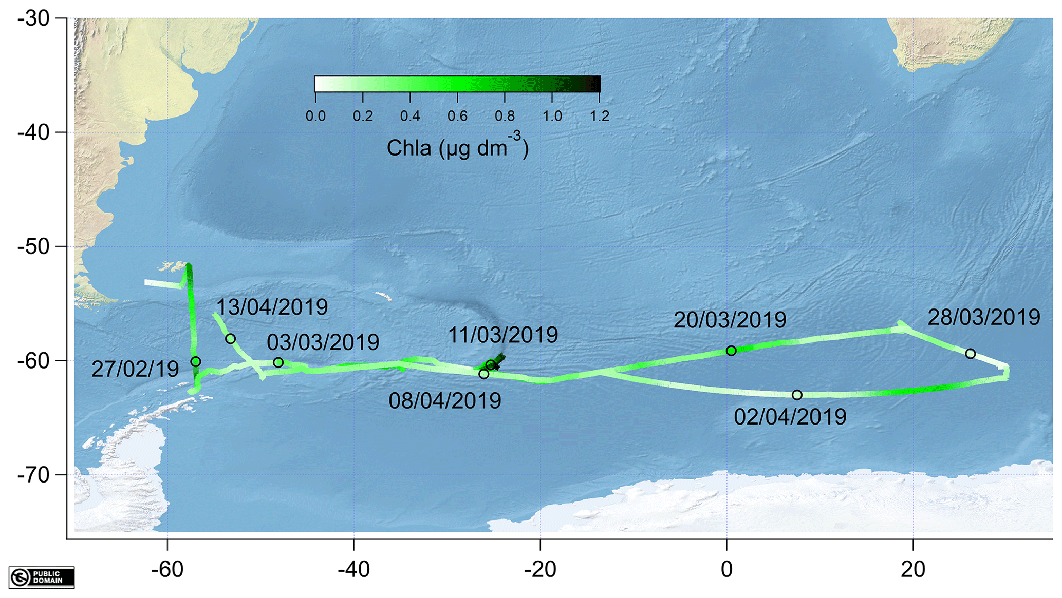
Figure 1 Map showing the cruise track coloured by underway chlorophyll a (chl a) with sampling dates indicated as black circles. All the data were created from public domain GIS data found on the Natural Earth website (http://www.naturalearthdata.com, last access: 8 May 2020). They were read into Igor using the Igor GIS XOP beta.

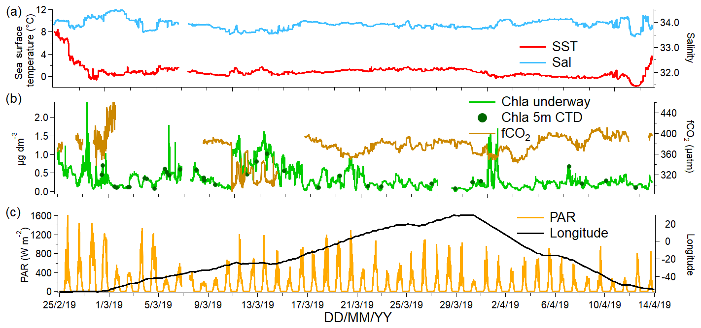
Figure 2 (a) Sea surface temperature and surface salinity, (b) chlorophyll a concentrations measured underway and from the sensor installed on the CTD sensor at 5 m depth as well as underway fCO₂, and (c) photosynthetic active radiation along with the longitude measured along the cruise track.

2.2 VOC measurements

During ANDREXII, VOCs in seawater and ambient air were measured with a proton-transfer-reaction mass spectrometer (PTR-MS, high-sensitivity model by Ionicon). To measure seawater concentrations, a segmented flow coil equilibrator (SFCE) was used to equilibrate underway seawater with “zero air” (Wohl et al., 2019). The underway seawater inlet of the JCR is situated at approximately 5–7 m depth and set flush with the hull. The SFCE nominally sampled from the bottom of a small (ca. 200 cm³) glass vessel that was overflowing rapidly with underway seawater. In addition to the underway measurements, approximately once a day seawater sampled from the 5 m Niskin bottle from the CTD was measured to verify that the ship's underway seawater inlet did not affect the measured concentrations. There was no significant difference in VOC concentration sampled from the underway seawater inlet and the 5 m Niskin bottle (t test, n=35, p<0.05).

A thermometer was installed at the seawater exhaust of the SFCE to continuously measure the seawater temperature. This revealed that when using the SFCE continuously with very cold seawater (cruise mean SST 1 ^∘C) and zero-air cylinders mounted outside on deck, the seawater temperature in the coil only reached 18 ^∘C (despite the water bath holding the SFCE being set to 25 ^∘C). This is in contrast to earlier laboratory measurements and an Arctic deployment, during which the water exiting the SFCE was always 20 ^∘C with the zero-air cylinder housed inside the lab. The continuously recorded temperature was used to calculate the Henry solubility and hence the seawater concentrations for this cruise. SFCE calibrations using Milli-Q water (20 ^∘C) and cold seawater revealed that these gases fully equilibrated regardless of the initial temperature (see Appendix A).

An air inlet was installed on a 40 cm pole extending forward from the railing of the walkway in front of the ship's bridge at approximately 16 m above the ocean surface. Ambient air was drawn towards the PTR-MS via a ∼90 m PTFE (polytetrafluoroethylene) air sampling tube (o.d. 9.5 mm, wall thickness 1.5 mm) using a Vacuubrand MD 4 NT diaphragm pump at a flow rate of circa 30 dm³ min⁻¹. The sampling tube followed a complex path around the ship, had a number of tight turns, and was mostly sheltered from direct sunlight. The PTR-MS subsampled from this air sampling tube upstream of the pump at a flow of approximately 100 cm³ min⁻¹. We do not expect large aerosols to make it to the PTR-MS because of the tight turns in the main sampling tube as well as the low subsample flow. The residence time of ambient air in the sampling tube was approximately 6 s. The blank measurements for ambient air mixing ratios were made by diverting ambient air through a custom-made platinum(Pt) catalyst at 450 ^∘C. The high efficiency of this Pt catalyst at oxidizing all VOCs in air to CO₂ has been demonstrated elsewhere (Yang and Fleming, 2019).

PTFE solenoid valves (1∕8 in. = 3.175 mm, Takasago Fluidic Systems) controlled by the PTR-MS were used to create an hourly measurement cycle of 40 min SFCE headspace (proportional to seawater concentration), 5 min ambient air scrubbed by the Pt catalyst at 450 ^∘C (catalyst blank), and 15 min of ambient air measurements.

2.2.1 Calibrations

The PTR-MS was calibrated weekly during the cruise using a certified gas calibration standard and two mass flow controllers to produce dynamic calibrations (Apel Riemer Environmental Inc., Miami, Florida, USA; nominal volume mixing ratio of 500 ppbv for acetaldehyde, methanol, acetone, isoprene DMS, benzene, toluene). Calibration slopes were typically within 10 % of each other.

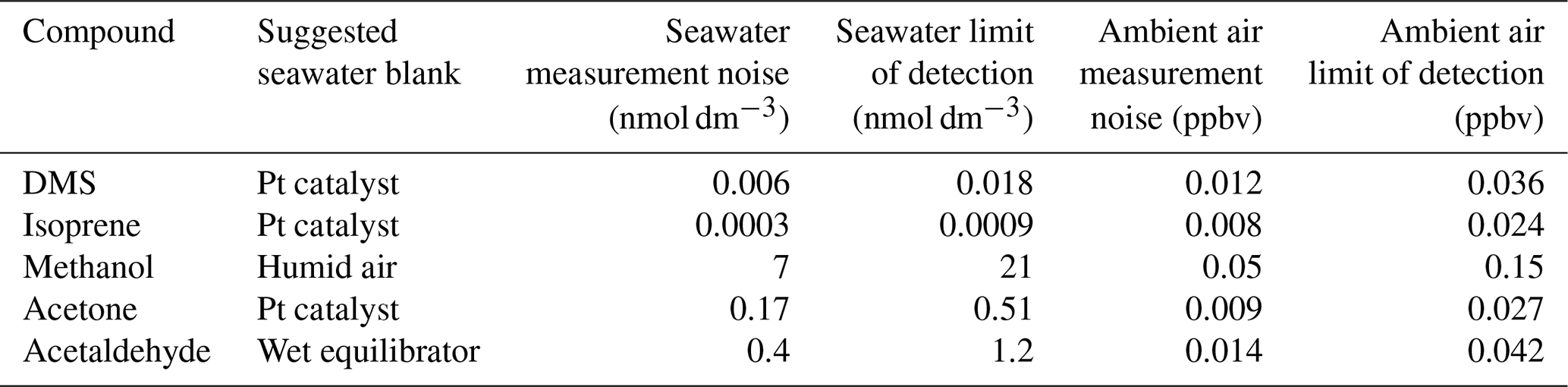
A lower PTR-MS drift tube voltage of 640 V was applied during this cruise compared to Wohl et al. (2019), while other PTR-MS settings were kept the same. Thus the humidity dependence of the signal and the background was slightly different from those of Wohl et al. (2019) as determined during the cruise. The background measurement of methanol and possibly acetaldehyde showed a humidity dependence at 640 V. The calibration slope for isoprene was corrected for its humidity dependence using a fragmentation ratio specifically determined at 640 V in the PTR-MS (Wohl et al., 2019). The other VOCs did not show a humidity dependence in either the slope or background. Several different types of blanks were measured in order to compute the seawater concentrations (Sect. S1 in the Supplement). Due to the aforementioned humidity dependence in the background of methanol and acetaldehyde, we used blanks that were measured at the same humidity as the equilibrator headspace for those two VOCs (Table 1). For compounds that do not display a humidity dependence in the background, hourly measurement of ambient air scrubbed by the Pt catalyst was used as a seawater blank because of its high frequency.

Table 1 Seawater blank used for each compound during this deployment. Hourly measurement noise (1σ) and limit of detection (3σ) of seawater and ambient air measurement are listed and were determined as described in the text.

Two methods were used to determine the SFCE calibration slopes for seawater methanol, acetone, and acetaldehyde concentrations during this cruise: invasion and evasion. In evasion calibrations, pure solvents were dissolved by serial dilution in Milli-Q water and seawater as described previously (Wohl et al., 2019). These diluted standards were measured with the SFCE-PTR-MS system using the same procedure as for seawater samples. During invasion experiments, a known amount of certified gas standard was added to the carrier gas, which was equilibrated with essentially VOC-free Milli-Q water or very deep seawater.

For the fully equilibrating gases, the calibration slopes are proportional to the Henry gas solubility (H). Invasion and evasion experiments represent independent estimates of solubility of these gases at environmentally relevant concentrations. For acetone and methanol, our invasion and evasion calibrations agreed only if we divide their recommended solubilities (Burkholder et al., 2015) by 1.4 and 1.6 respectively (see Appendix A). We use these experimentally determined H values to compute the concentrations, saturations, and fluxes of acetone and methanol here. The reference of Burkholder et al. (2015) is used here since it represents a critical tabulation of the latest experimental data. The solubilities inferred by our study are within the range of previously published solubilities.

As with previous calibrations, these on-board measurements showed that the SFCE achieved essentially full (i.e. 100 %) equilibration for all the VOCs measured here except for isoprene (Wohl et al., 2019). The equilibration efficiency of isoprene was determined to be 87±9 % (±1σ) from onboard invasion experiments. This is higher than the equilibration efficiency observed during our earlier laboratory tests, probably due to the higher seawater flow (120 instead of 100 cm³ min⁻¹) used on this cruise. We use this measured equilibration efficiency to determine seawater isoprene concentrations.

2.2.2 Limit of detection estimates

Measurement uncertainty and limit of detection (LOD) of this system have already been described in Wohl et al. (2019). Here we reassess the LOD of our seawater and ambient air measurements. This is to address the possibilities that (i) our previous estimates (Wohl et al., 2019) might have represented an overidealized case and (ii) the LOD is dependent on the PTR-MS quadrupole settings, dwell times (Yang et al., 2013c), and calibration slopes (Wohl et al., 2019), which may differ between deployments. The most appropriate seawater background for the ANDREXII cruise is listed in Table 1. The mean of the 5 min Pt-catalyst blank measurements was interpolated over the time series of measurements. The standard deviation of the detrended blanks (after subtracting the interpolation) was multiplied by the gas-phase calibration and represents the measurement noise (1σ) in parts per billion by volume of the ambient air measurement. To calculate the measurement noise of the seawater concentration, this mixing ratio was converted to a seawater concentration in the same way as the seawater measurement (Wohl et al., 2019). The LOD was defined as 3σ. The underway ambient air and seawater data were also first averaged to 5 min means, with each hourly average containing six continuous 5 min means of equilibrator headspace and two continuous 5 min means of ambient air measurements (i.e. the first minutes after automated valve switch were discarded to account for residual air in the tubing). The measurement noise derived from this analysis was divided by the square root of the number of 5 min measurements in each hourly cycle to calculate the hourly measurement noise and limit of detection, which are listed in Table 1.

2.2.3 Light-driven contamination in the seawater measurement

The SFCE was installed near the starboard windows in the main lab. During the early part of the cruise, intense sunlight sometimes shined directly at the SFCE. This led to observations of extremely high headspace mixing ratios that were presumably due to photochemical production within the SFCE. This effect disappeared instantly after covering the air–water separating tee from direct sunlight. The air–water separating tee of the SFCE was thereafter covered from direct sunlight and the blinds were kept closed from 4 March 2019 onwards. The effect of this light reduction measure is illustrated in Fig. 3. Hence, daytime seawater concentrations of acetaldehyde, acetone, and isoprene prior to 4 March 2019 were not used in further analysis. Daytime data after 4 March 2019 did not show any dependence on the ship's heading, indicating that this artefact had been satisfactorily dealt with. The exact cause of this light-driven contamination in the SFCE system is unclear. Photochemical production of isoprene and carbonyl compounds at the sea surface microlayer has been observed before (Brüggemann et al., 2018; Ciuraru et al., 2015). It could be that similar reactions were taking place on the water surfaces inside of the SFCE.

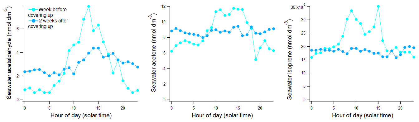
Figure 3 Underway seawater concentrations binned in 24-hourly bins for the week before and 2 weeks after protecting the SFCE equilibrator from sunlight on 4 March 2019.

2.2.4 Filtering of atmospheric VOC measurements

Ambient air measurements were filtered to remove the influence of ship stack contamination. Firstly, all measurements made during a sampling cycle were discarded if the concentration of benzene or toluene was above a threshold of 0.2 ppbv. This was to eliminate small-scale contamination from the ventilation pipes on the foremast. Secondly, data were discarded if the relative wind speed was less than 4 m s⁻¹. Thirdly, only ambient air measurements with the wind coming from 10 to 70^∘ either side of the bow were used for further analysis. Filtering was carried out using 1 min averaged wind measurements from a Metek sonic anemometer installed on the foremast and resulted in the removal of 55 % of the ambient air measurements.

2.3 Flux calculations

The saturation (%Sat) of the surface ocean relative to the atmosphere is calculated using Eq. (1).

$$\begin{array}{}\text{(1)}& \mathit{\%}\mathrm{Sat}=\left({\displaystyle \frac{C_{\mathrm{w}}}{C_{\mathrm{a}}\cdot H}}\right)\cdot \mathrm{100}\end{array}$$

Here a saturation above 100 % corresponds to oceanic outgassing. H is the dimensionless liquid over gas form of the Henry solubility.

The net air–sea flux (F, positive from sea to air) is determined using the two-layer model flux equation (Liss and Slater, 1974) illustrated in Eq. (2).

$$\begin{array}{}\text{(2)}& F=k\cdot \left(C_{\mathrm{w}}-H\cdot C_{\mathrm{a}}\right)\end{array}$$

Here the gas transfer velocity (k) is defined by Eq. (3).

$$\begin{array}{}\text{(3)}& k={\displaystyle \frac{\mathrm{1}}{\frac{\mathrm{1}}{k_{\mathrm{w}}}+\frac{H}{k_{\mathrm{a}}}}}\end{array}$$

To calculate the air-side (k_a) transfer velocity, we use the following parametrization derived from direct measurements of air–sea methanol transfer (Yang et al., 2013a) (Eq. 4). This was chosen to be the k_a for all VOCs of concern since we do not expect them to differ by more than ∼10 %:

$$\begin{array}{}\text{(4)}& k_{\mathrm{a}}=\mathrm{8814}{u}_{\ast }+\mathrm{6810}{u}_{\ast }^{\mathrm{2}}.\end{array}$$

Here the friction velocity u_∗ is simplistically calculated using the parameterization from Johnson (2010) (Eq. 5).

$$\begin{array}{}\text{(5)}& u_{\ast }=u_{\mathrm{10}}\cdot \sqrt{\mathrm{1.3}\times {\mathrm{10}}^{-\mathrm{3}}}\end{array}$$

Wind speed from a Metek sonic anemometer was adjusted to 10 m height (u₁₀). For isoprene, the waterside transfer velocity (k_w) is calculated using the parameterization by Nightingale et al. (2000) (Eq. 6).

$$\begin{array}{}\text{(6)}& k_{\mathrm{w}}=\left(\mathrm{0.222}\cdot u_{\mathrm{10}}^{\mathrm{2}}+\mathrm{0.333}\cdot u_{\mathrm{10}}\right)\cdot {\left({\displaystyle \frac{{\mathit{Sc}}_{\mathrm{w}}}{{\mathit{Sc}}_{\mathrm{600}}}}\right)}^{-\mathrm{0.5}}\end{array}$$

Sc_w is the waterside Schmidt number and Sc₆₀₀ is the Schmidt number of 600. This parametrization most likely represents an overestimation of k_w for gases that have similar or greater solubility than DMS because of the solubility dependence in bubble-mediated gas exchange (Yang et al., 2011). Thus for DMS, acetaldehyde, acetone, and methanol, mean k_w determined from DMS measurements from five different cruises was used here (Yang et al., 2011) and scaled to the ambient temperature assuming ${\mathit{Sc}}_{\mathrm{w}}^{-\mathrm{0.5}}$.

The water-phase Schmidt numbers (Sc_w) of methanol, acetone, acetaldehyde, and DMS are determined following Johnson (2010). The Schmidt number of isoprene is calculated using the equation presented in Palmer and Shaw (2005). Henry solubility values are converted from freshwater to seawater using the method presented by Johnson (2010). Methanol and acetone concentrations, fluxes, and saturations are calculated using the experimentally determined solubility presented in Appendix A.

3 Underway ambient air mixing ratios, seawater concentrations, and air–sea fluxes

In the following subsections, the ambient air and seawater concentrations of DMS, isoprene, methanol, acetone, and acetaldehyde as well as their saturations and fluxes are discussed. Saturations below 100 % indicate undersaturation in seawater (i.e. air-to-sea or negative flux). Two versions of fluxes are presented: fluxes when both ambient air and seawater data were available during an hourly measurement cycle and continuous flux estimates despite missing ambient air data (e.g. wind direction out of sector), which are estimated by smooth interpolation of the ambient air mixing ratios.

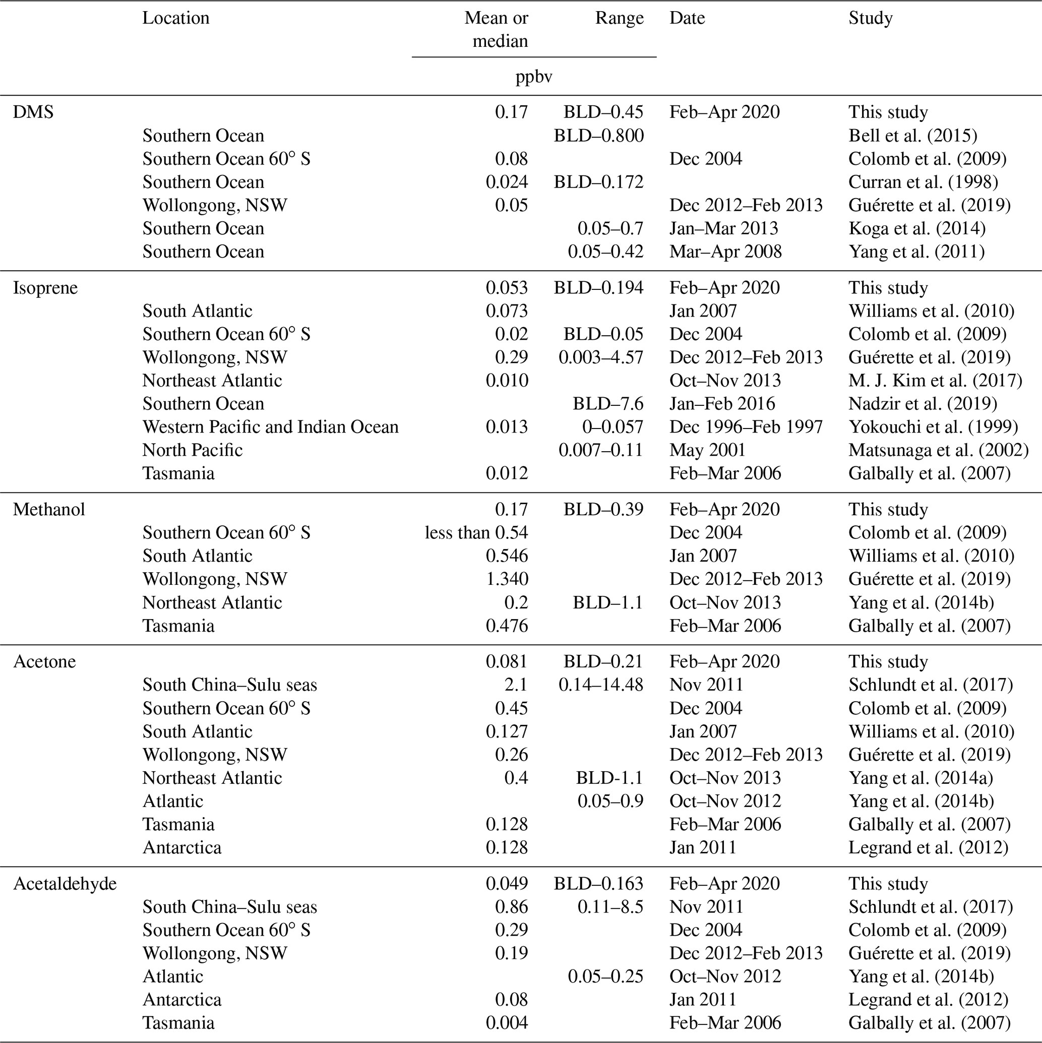
As a quick overview and for reference, cruise mean ambient air and seawater concentrations are presented in Table 2. Cruise mean saturations and calculated fluxes are shown in Table 3. Also included are the median and quantiles as well as the standard deviation. We also show two tables (Tables 4 and 5) summarizing some previous ambient marine air and seawater measurements of these compounds. These tables do not represent comprehensive reviews of previously published measurements, but instead aid comparison of our measurements to previous measurements from the Southern Ocean and other regions.

Table 2 Cruise mean seawater concentration (nmol dm⁻³) and ambient air mixing ratio (ppbv). Cruise median and quantiles (Q₂₅ and Q₇₅) are also indicated as well as the standard deviation (SD).

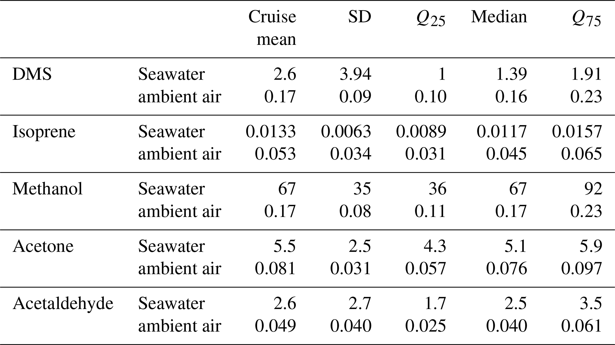
Table 3 Cruise mean saturation (%) and flux (µmol m⁻² d⁻¹). These calculations are only fluxes and saturations for which ambient air and seawater measurements were both available during the same hourly measurement cycle. Saturations below 100 % indicate undersaturation, and a negative flux indicates flux from the air into the ocean. Campaign median and quantiles (Q₂₅ and Q₇₅) are also indicated as well as the standard deviation (SD).

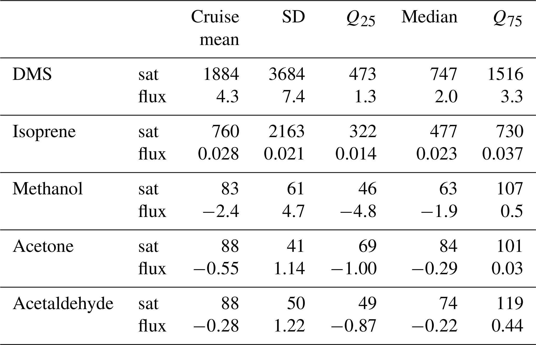
Table 4 Table summarizing previous surface seawater measurements of DMS, isoprene, methanol, acetone, and acetaldehyde in the Southern Ocean and other regions (BLD is below limit of detection).

Table 5 Table summarizing previous marine ambient air measurements of DMS, isoprene, methanol, acetone, and acetaldehyde in the Southern Ocean and other regions (BLD is below limit of detection).

3.1 Dimethyl sulfide

The time series of DMS ambient air and seawater concentrations as well as the corresponding fluxes and saturations are presented in Fig. 4.

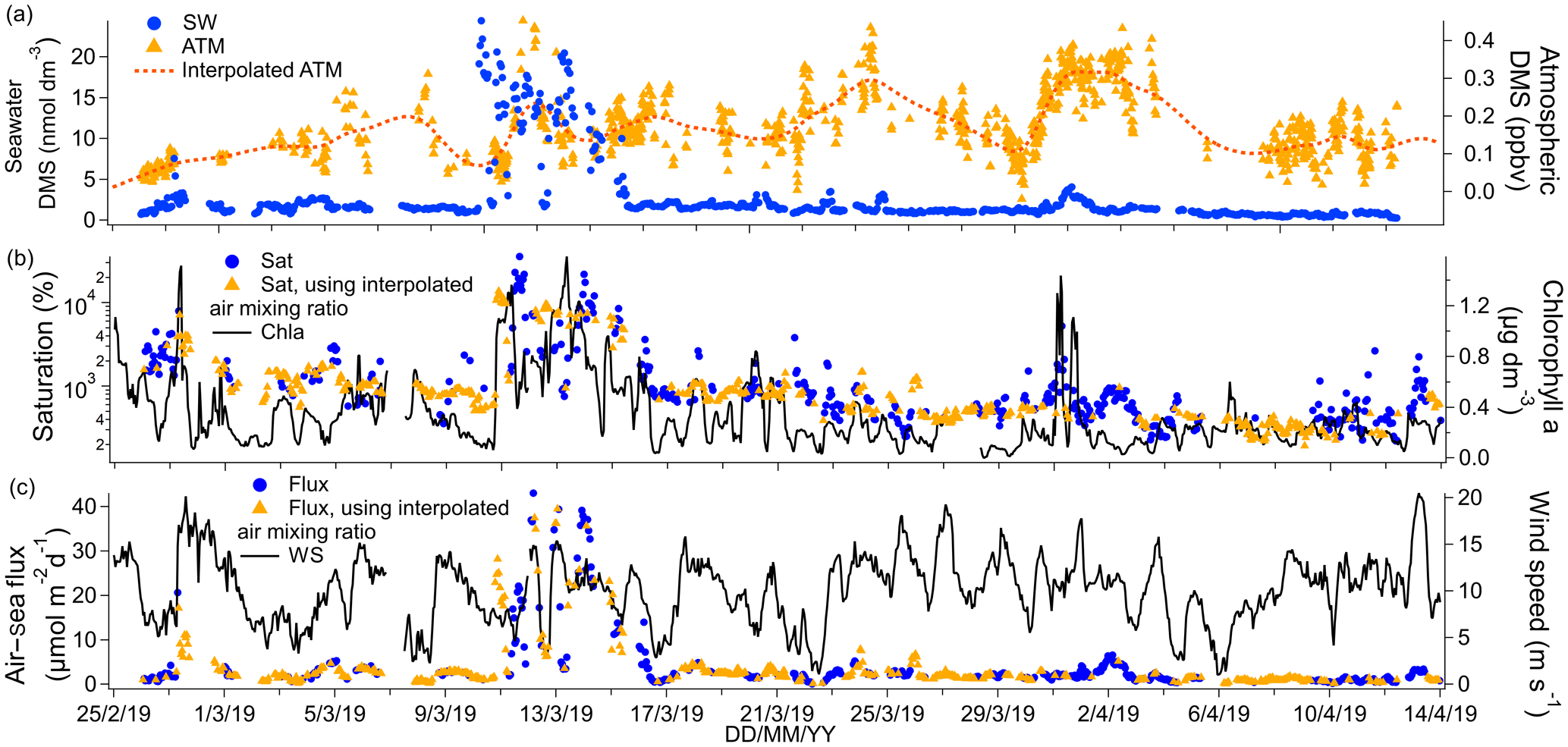
Figure 4 (a) Time series of DMS seawater (SW) concentrations as well as measured and interpolated marine boundary layer air mixing ratios (ATM and interpolated ATM). (b) Time series of DMS saturations determined using the measured air mixing ratio and interpolated air mixing ratio and time series of chlorophyll a. (c) Time series of air–sea DMS fluxes calculated using the measured air mixing ratio and interpolated air mixing ratio and time series of wind speed.

The campaign mean seawater concentration of DMS was 2.60 nmol dm⁻³ and the median was 1.39 nmol dm⁻³. This illustrates the positive skewness of the DMS seawater concentrations due to episodic high concentrations of DMS. The highest DMS seawater concentrations were observed near the Antarctic Peninsula upwelling region (around 28 February 2019, up to 7.55 nmol dm⁻³) and east of the South Sandwich Islands (around 13 March 2019, up to 24.44 nmol dm⁻³). Chlorophyll a was also elevated in those regions. These and other fine-scale hotspots of DMS were well resolved due to our use of continuous and fast-responding measurements. To remove the effect of ship sampling bias on the overall cruise mean (e.g. spending multiple days surveying a plankton bloom), the DMS concentrations were first averaged in 1^∘ longitudinal bins. The mean of spatially averaged seawater DMS concentration for this campaign was 1.87 nmol dm⁻³ (confidence interval of the mean: 1.46–2.28 nmol dm⁻³). This is similar to the Lana et al. (2011) climatology in this region and during these months (average of 1.5 nmol dm⁻³ and range of 0–3 nmol dm⁻³).

Cruise mean and median ambient air mixing ratios of DMS were 0.17 and 0.16 ppbv respectively. These values are comparable to previous measurements over the Southern Ocean at this time of year (Bell et al., 2015; Colomb et al., 2009; Curran et al., 1998; Guérette et al., 2019; Koga et al., 2014; Yang et al., 2011). Ambient air mixing ratios were up to about 0.5 ppbv on occasion and did not correlate with seawater concentrations. This is probably because air parcels travel much faster than seawater, leading to a decoupling between air and sea DMS concentrations.

The campaign mean DMS flux was 4.3 µmol m⁻² d⁻¹. Fluxes were typically <7 µmol m⁻² d⁻¹ but exceeded 30 µmol m⁻² d⁻¹ within the phytoplankton bloom encountered on around 13 March 2019. Our mean DMS flux compares well to direct measurements of DMS flux over the Southern Ocean (Bell et al., 2015; Yang et al., 2011). Averaging the DMS flux in 1^∘ longitudinal bins (as with the seawater concentration above) results in a spatial mean flux of 3.2 µmol m⁻² d⁻¹. From now on we discuss only temporal statistics.

3.2 Isoprene

The time series of isoprene ambient air and seawater concentrations as well as the corresponding fluxes and saturations are presented in Fig. 5.

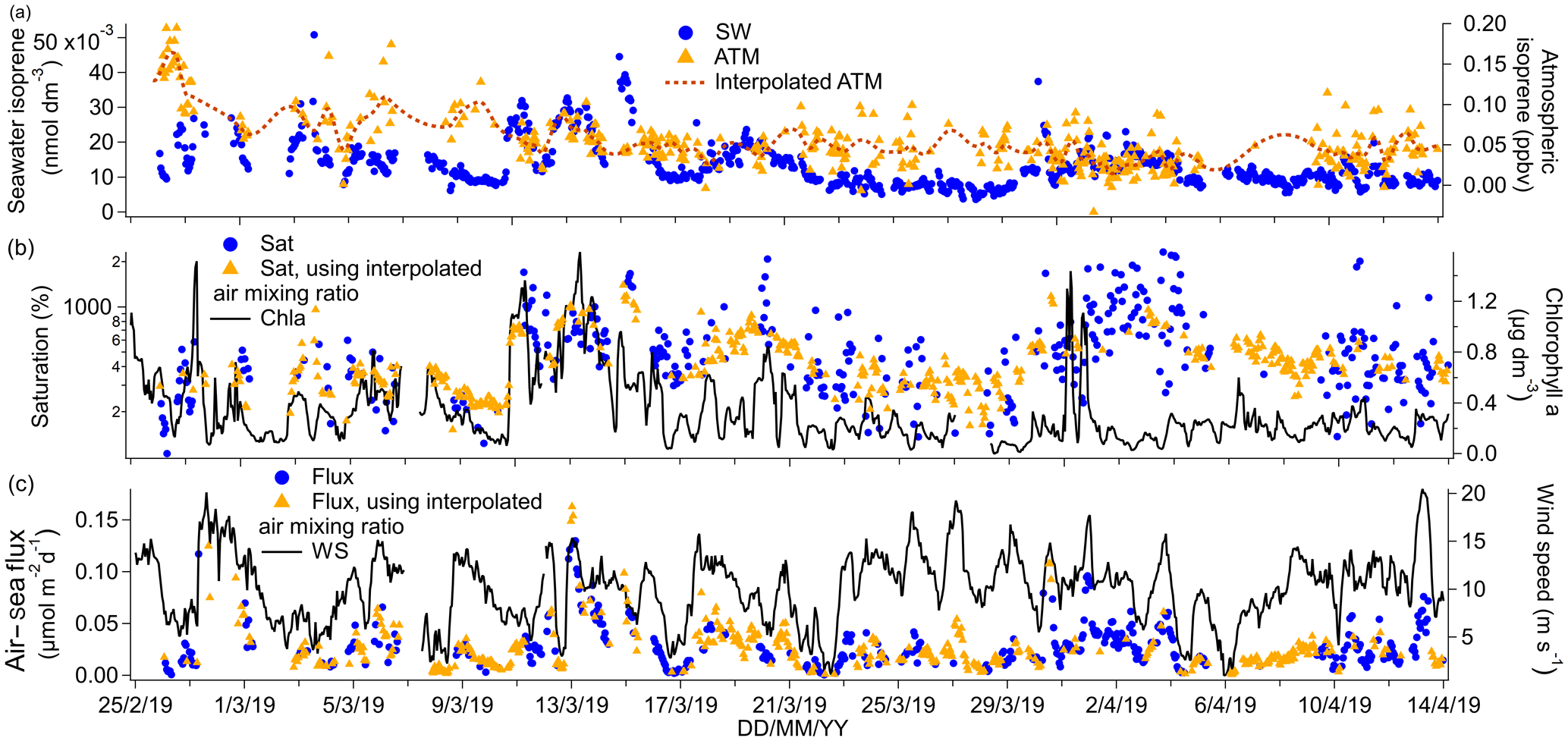
Figure 5 (a) Time series of isoprene seawater (SW) concentrations as well as measured and interpolated marine boundary layer air mixing ratios (ATM and interpolated ATM). (b) Time series of isoprene saturations determined using the measured air mixing ratio and interpolated air mixing ratio and times series of chlorophyll a. (c) Time series of air–sea isoprene fluxes calculated using the measured air mixing ratio and interpolated air mixing ratio and time series of wind speed.

The campaign mean isoprene seawater concentration was 0.0133 nmol dm⁻³. This is comparable to previous measurements in the open ocean (Hackenberg et al., 2017; Ooki et al., 2015) and also in the Southern Ocean (Kameyama et al., 2014). Isoprene concentrations as high as 0.040 nmol dm⁻³ were observed near the Antarctic Peninsula and in the phytoplankton bloom near the South Sandwich Islands. As shown in Figs. 2 and 5, these areas were also associated with high chlorophyll a concentration and low fCO₂.

The linear regression between underway isoprene (nmol dm⁻³) and chlorophyll a (µg dm⁻³) yielded a slope of 0.0136 nmol dm⁻³ isoprene (µg chl a dm⁻³)⁻¹ with an R² value of 0.35 and an intercept of 0.0087 nmol dm⁻³ isoprene (P=0.000, N=799). There also appears to be a first-order relationship between chlorophyll a and seawater isoprene concentrations in other oceanic basins, with variable R² values of 37 % (Kameyama et al., 2014), 12 % (Baker et al., 2000), and 52 % (Broadgate et al., 1997). The regression slope from our campaign, where SST was generally between 0 and 2 ^∘C, compares best to previous measurements in colder waters. For example, Ooki et al. (2015) have found a slope of 0.0143 nmol dm⁻³ isoprene (µg chl a dm⁻³)⁻¹ and intercept of 0.00223 nmol dm⁻³ isoprene in waters with temperatures between 3.3 and 17 ^∘C. Hackenberg et al. (2017) have found slopes of 0.0379 nmol dm⁻³ isoprene (µg chl a dm⁻³)⁻¹ and 0.0341 nmol dm⁻³ isoprene (µg chl a dm⁻³)⁻¹ for SST below 20 ^∘C in the Atlantic and Arctic oceans respectively. The slope between chlorophyll a and isoprene concentration appears to increase in steepness with temperature (Hackenberg et al., 2017; Ooki et al., 2015).

Our dataset showed a significant negative correlation between seawater isoprene and fCO₂ (slope: −0.00015 nmol dm⁻³ isoprene (µatm fCO₂)⁻¹, intercept: 0.0699 nmol dm⁻³ isoprene, R²=0.44, P=0.000, N=690). This might be because isoprene is produced by phytoplankton (Dani and Loreto, 2017; Shaw et al., 2010), and high biological productivity tends to reduce seawater fCO₂ in phytoplankton blooms (Blain et al., 2007; Wingenter et al., 2004). A negative correlation between the partial pressure of CO₂ (pCO₂, whether temperature-normalized or not) and seawater isoprene concentrations has been reported previously (Kameyama et al., 2014), but this correlation only held for waters south of 53^∘ S. In the study of Kameyama et al. (2014), the SST normalized pCO₂ was viewed as a proxy for net community production.

The mean ambient air mixing ratio of isoprene on this cruise was 0.053 ppbv and the median was 0.045 ppbv, illustrating a positive skewness in the isoprene ambient air mixing ratio. This positive skewedness is probably caused by biology- and wind speed-dependent emissions as well as the short lifetime of isoprene in the atmosphere that prevents it from being more fully mixed. Positively skewed atmospheric isoprene mixing ratios have also been observed previously over the ocean (M. J. Kim et al., 2017). The mean of our measurements compares best to previous measurements over the Southern Ocean (Colomb et al., 2009; Nadzir et al., 2019; Yokouchi et al., 1999) as well as other biologically productive areas (Shaw et al., 2010). The underway isoprene air and water concentrations presented here show a small but statistically significant difference between daytime and night-time, which will be discussed further in Sect. 4.

Isoprene was supersaturated by 760 % in the mean. The large supersaturation and low solubility of isoprene suggest that ambient air mixing ratios influence isoprene saturation levels very little. A mean isoprene flux of 0.028 µmol m⁻² d⁻¹ is computed for this deployment, which exceeded 0.07 µmol m⁻² d⁻¹ on occasion. Our fluxes compare well to some published estimates from other oceans (Baker et al., 2000; Tran et al., 2013), but they are about 10-fold lower than an estimate from the Southern Ocean by Kameyama et al. (2014). This is probably due to the lower seawater concentrations measured during our campaign compared to the seawater concentrations reported by Kameyama et al. (2014). Our fluxes are also comparable to direct flux measurements in the Labrador Sea where mean isoprene fluxes were found to be dominated by episodic emissions (M. J. Kim et al., 2017).

3.3 Methanol

The time series of methanol ambient air and seawater concentrations as well as the corresponding fluxes and saturations are presented in Fig. 6.

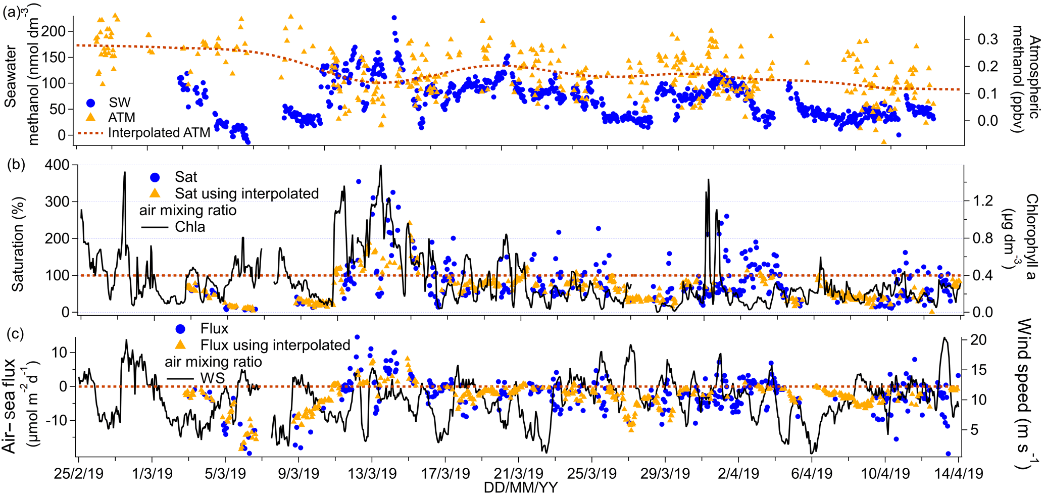
Figure 6 (a) Time series of methanol seawater (SW) concentrations as well as measured and interpolated marine boundary layer air mixing ratios (ATM and interpolated ATM). (b) Time series of methanol saturations determined using the measured air mixing ratio and interpolated air mixing ratio and time series of chlorophyll a. (c) Time series of air–sea methanol fluxes calculated using the measured air mixing ratio and interpolated air mixing ratio and time series of wind speed.

Median and mean seawater methanol concentrations were the same at 67 nmol dm⁻³. These are higher than previous high-latitude measurements in the South Atlantic during austral spring (Beale et al., 2013; Yang et al., 2014b) and in the Labrador Sea in late boreal autumn (Yang et al., 2014a), and they are similar in magnitude to measurements in parts of the North Atlantic during the boreal autumn (Beale et al., 2013). The highest seawater methanol concentrations of up to 226 nmol dm⁻³ were observed in the phytoplankton bloom encountered around 13 March 2019. Interestingly, the range of observations on this cruise (below detection to 226 nmol dm⁻³) encompasses a broad range of previously published values of 15 to 361 nmol dm⁻³ in tropical and temperate waters (Beale et al., 2013, 2015; Kameyama et al., 2009; Williams et al., 2004; Yang et al., 2013a, 2014a). The large range in seawater methanol concentrations highlights the advantage of our high-frequency measurement system.

Regression analysis of seawater concentrations of methanol against isoprene gave a significant positive relationship (slope: 3524 nmol dm⁻³ methanol (nmol dm⁻³ isoprene)⁻¹, intercept: 22 nmol dm⁻³ methanol, R²=0.38, P=0.000, N=771). Furthermore, methanol significantly correlated with fCO₂ (slope: −1.0 nmol dm⁻³ methanol (µatm fCO₂)⁻¹, intercept: 450 nmol dm⁻³ methanol, R²=0.58, P=0.000, N=651), which suggests production of methanol by phytoplankton. However, seawater methanol concentrations did not correlate significantly with chlorophyll a, which is consistent with previous seawater measurements in the Atlantic (Yang et al., 2014b).

The correlation between methanol and isoprene on our cruise suggests that both compounds may be produced by similar phytoplankton species. Measurements of laboratory phytoplankton cultures show that cyanobacteria (Synechococcus and Trichodesmium) are strong producers of isoprene (Bonsang et al., 2010) but weak producers of methanol (Mincer and Aicher, 2016). In contrast, Phaeodactylum, a temperate diatom, was found to produce large amounts of methanol (Mincer and Aicher, 2016) but moderate amounts of isoprene (Bonsang et al., 2010). Emiliania huxleyi, a coccolithophore, was observed to produce moderate amounts of both isoprene and methanol (Bonsang et al., 2010; Mincer and Aicher, 2016). Unfortunately no plankton composition measurements were made during our cruise so we are unable to comment further.

Ambient air mixing ratios of methanol were very low (mean = 0.17 ppbv, median = 0.17 ppbv), in agreement with previous measurements in the Southern Hemisphere of about 0.2 ppbv in the South Atlantic (Yang et al., 2013a) and up to 0.54 ppbv above the southern Indian Ocean (Colomb et al., 2009). Lower ambient air mixing ratios of methanol in the Southern Hemisphere compared to the Northern Hemisphere are probably due to the relatively sparse land mass and vegetation coverage (Yang et al., 2013a).

The Southern Ocean was a net sink of methanol on average with a mean saturation of 83 % and flux of −2.4 µmol m⁻² d⁻¹. The presence of occasional waters with high methanol concentrations, combined with relatively low ambient air mixing ratios, led to episodes of outgassing of methanol over phytoplankton blooms (up to ∼ 10 µmol m⁻² d⁻¹). Net sea-to-air transfer of methanol is somewhat unexpected given the extremely high solubility of methanol. Previous direct flux measurements of methanol along a meridional transect through the Atlantic (Yang et al., 2013a) and in the Labrador Sea (Yang et al., 2014a) have shown that the net flux of methanol was consistently into the ocean, with the largest air-to-sea flux in regions downwind of continents. Outgassing of methanol from the ocean has been suggested previously for some waters of the North Atlantic (Beale et al., 2013). In our calculation, we note that the methanol flux is insensitive to the choice of solubility. If we instead calculated the methanol flux and seawater methanol concentrations using the recommended solubility by Burkholder et al. (2015), the mean seawater concentration of methanol would have been 60 % higher, while the saturation and flux would have remained unchanged. Saturation and flux remain unchanged since seawater concentration and solubility change by the same factor and the two changes cancel out.

3.4 Acetone

The time series of acetone ambient air and seawater concentrations as well as the corresponding fluxes and saturations are presented in Fig. 7.

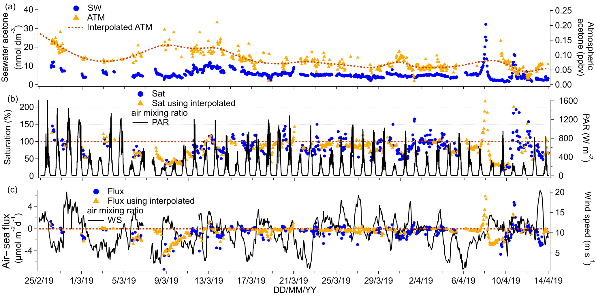
Figure 7 (a) Time series of acetone seawater (SW) concentrations as well as measured and interpolated marine boundary layer air mixing ratios (ATM and interpolated ATM). (b) Time series of acetone saturations determined using the measured air mixing ratio and interpolated air mixing ratio and time series of chlorophyll a. (c) Time series of air–sea acetone fluxes calculated using the measured air mixing ratio and interpolated air mixing ratio and time series of wind speed.

The mean (±1σ) seawater acetone concentration was 5.5±2.5 nmol dm⁻³, while the median was 5.1 nmol dm⁻³. These values compare well to previous measurements of less than 10 nmol dm⁻³ in the South Atlantic (Beale et al., 2013; Yang et al., 2014b) and in the Labrador Sea (Yang et al., 2014a). Seawater acetone concentrations from this cruise are also similar to other open-ocean measurements (Hudson et al., 2007; Kameyama et al., 2010; Marandino et al., 2005; Schlundt et al., 2017). Unlike methanol, seawater acetone concentration was usually quite consistent and ranged from 4.3 (lower quantile) to 5.9 (upper quantile).

A significant negative correlation of acetone with fCO₂ is observed (slope: −0.053 nmol dm⁻³ acetone (µatm CO₂)⁻¹, intercept: 26.51 nmol dm⁻³ acetone, R²=0.58, P=0.000, N=671), excluding high seawater acetone measurements from 8 and 10 April 2019. These elevated data are considered strong outliers (higher than the upper quantile plus 3 times the interquartile range) for reasons currently unknown. This correlation of acetone with fCO₂ suggests a possible role a biology in the production of acetone. Previous investigators have found correlations between seawater acetone concentration and the abundance of haptophytes and pelagophytes (Schlundt et al., 2017), suggesting direct production by phytoplankton and/or bacterial communities associated with these phytoplankton. Taddei et al. (2009) have also observed higher emission of acetone in high-chlorophyll a areas in the remote South Atlantic. Our acetone data showed a weak, although significant, positive correlation with chlorophyll a concentration (slope: 4.84 nmol dm⁻³ acetone (µg chl a)⁻¹, intercept: 4.11 nmol dm⁻³ acetone, R²=0.07, P=0.000, N=750). Despite this, the main source of acetone in seawater is probably photochemical production, which has been found to account for up to 100 % of gross production rates of acetone in seawater (Dixon et al., 2013). The underway acetone air and water concentrations presented here show a small but statistically significant difference between daytime and night-time, which will be discussed further in Sect. 4.

The mean (±1σ) ambient air mixing ratio of acetone measured during this cruise was very low (mean of 0.081±0.031 ppbv and median 0.076 ppbv). This compares well with clean marine air measurements of 0.188 ppbv at Cape Grim, Tasmania (Galbally et al., 2007), air coming off Antarctica with an average of 0.128 ppbv (Legrand et al., 2012), and marine air measurements with an average of 0.127 ppbv over the South Atlantic at 55^∘ S (Williams et al., 2010). The mean ambient air mixing ratio reported here is considerably lower than the modelled annual mean acetone air mixing ratio over the Southern Ocean of about 0.2 ppbv (Fischer et al., 2012). An updated global budget of acetone predicts slightly lower annual mean air mixing ratios over the Southern Ocean of 0.1–0.2 ppbv (Brewer et al., 2017). This decrease is largely due to an increased photolysis rate of acetone in the updated model (Brewer et al., 2017). Both of these works assume a fixed acetone seawater concentration of 15 nmol dm⁻³ (nearly 3 times our measurements) and so have the potential to overestimate air mixing ratios above the Southern Ocean. Further observations are needed to capture the seasonality of seawater acetone concentrations.

The mean seawater saturation of acetone was 88 %. Saturations of between 50 % and 200 % are typical for acetone (Schlundt et al., 2017; Yang et al., 2014a, b). A mean net flux into the ocean of −0.55 µmol m⁻² d⁻¹ suggests that the net flux of acetone is on average into the Southern Ocean this time of the year. Though occasional outgassing was also observed. Using a t test, the mean acetone flux was found to be significantly different from zero and the confidence interval of the campaign mean flux was −0.44 to −0.67 µmol m⁻² d⁻¹. The mean flux reported here is within the uncertainties of direct flux measurements of acetone over the Atlantic, which report a mean flux of −0.2 (propagated uncertainty 2.5) µmol m⁻² d⁻¹ (Yang et al., 2014b). The global budget of acetone suggests that the Southern Ocean is a weak sink for acetone (Fischer et al., 2012), in agreement with our measurements.

If we instead calculated the acetone flux and seawater acetone concentrations using the recommended solubility by Burkholder et al. (2015), the mean seawater concentration of acetone would have been 40 % higher, while the saturation and flux would have remained unchanged. The saturation and flux remain effectively unchanged, again because the mean concentration and solubility change by the same factor.

3.5 Acetaldehyde

The time series of acetaldehyde ambient air and seawater concentrations as well as the corresponding fluxes and saturations are presented in Fig. 8.

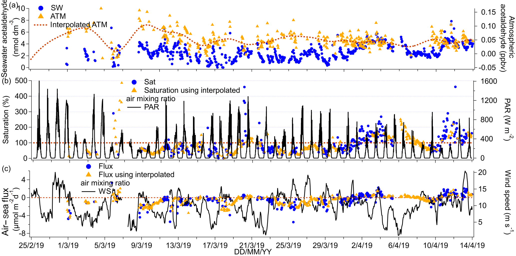
Figure 8 (a) Time series of acetaldehyde seawater (SW) concentrations as well as measured and interpolated marine boundary layer air mixing ratios (ATM and interpolated ATM). (b) Time series of acetaldehyde saturations determined using the measured air mixing ratio and interpolated air mixing ratio and time series of chlorophyll a. (c) Time series of air–sea acetaldehyde fluxes calculated using the measured air mixing ratio and interpolated air mixing ratio and time series of wind speed.

The cruise mean seawater concentration of acetaldehyde was 2.6 nmol dm⁻³, while the median concentration was 2.5 nmol dm⁻³, suggesting a normal distribution in concentrations. The seawater concentrations measured here were generally lower than 6 nmol dm⁻³, which compares well to other open-ocean measurements (Beale et al., 2013; Kameyama et al., 2010; Schlundt et al., 2017; Williams et al., 2004; Yang et al., 2014b; Zhu and Kieber, 2018) but is lower than measurements near the coast in the English Channel (Beale et al., 2015) and off the west coast of Florida (Mopper and Stahovec, 1986). No seawater concentrations of acetaldehyde were reported for the first 4 d of the deployment because of the longer time needed for acetaldehyde to be flushed from the tubing in the SFCE compared to the other VOCs. No significant correlations between seawater acetaldehyde concentrations with fCO₂ or with chlorophyll a were observed, possibly due to rapid biological consumption of acetaldehyde in seawater (Dixon et al., 2013) that prevents the build-up of significant concentrations.

Mean ambient air mixing ratios of acetaldehyde were low at 0.049 ppbv and showed limited variability. Our measurement compares well with the previous atmospheric measurements of Legrand et al. (2012), who observed an average of 0.08 ppbv acetaldehyde in ambient air off of the Antarctic continent. Our measurement is also consistent with the interhemispheric gradient in acetaldehyde concentrations, where lower ambient air mixing ratios of acetaldehyde are generally observed in the Southern Hemisphere (Galbally et al., 2007; Guérette et al., 2019; Yang et al., 2014b). We did not observe any correlation in the ambient air mixing ratios (1) among all the VOCs and (2) between atmospheric VOCs and atmospheric CO₂. This is in contrast to observations by Yang et al. (2014b), who have found that methanol, acetone, and acetaldehyde ambient air concentrations correlated between each other and with CO₂. These earlier air measurements were taken along a transatlantic cruise and were likely more impacted by continental emissions (Yang et al., 2014b). Acetaldehyde showed clear diurnal variability in both seawater and ambient air, which will be discussed in more detail in Sect. 4.

The mean (±1σ) saturation of acetaldehyde was 88 %, which is within the range of previously reported acetaldehyde saturations (Schlundt et al., 2017; Yang et al., 2014b). The mean net flux of acetaldehyde was −0.28 µmol m⁻² d⁻¹ and thus weakly into the Southern Ocean this time of the year. Using a t test, we calculated that the mean net flux was significantly different from zero with a confidence interval of the mean of −0.51 to −0.25 µmol m⁻² d⁻¹. Our calculated flux is within the uncertainties of direct flux measurements across the Atlantic of 0.6 (propagated uncertainty 2.5) µmol m⁻² d⁻¹ (Yang et al., 2014b) but is less than the calculated flux over the South China and Sulu seas at −10.11 µmol m⁻² d⁻¹ (Schlundt et al., 2017), probably due to the higher ambient air mixing ratios at this location. The fluxes from our cruise are similar in magnitude to the modelled acetaldehyde fluxes from the Southern Ocean by Wang et al. (2019), who predict that the Southern Ocean is near equilibrium with respect to acetaldehyde.

4 Diurnal variability in VOCs

Here we analyse our data for possible diurnal variability and look for light-driven sources and sinks for these compounds. Dixon et al. (2013) estimated that photochemical production accounts for up to 100 % and 68 % of the gross production rates of acetone and acetaldehyde respectively in seawater. Halsey et al. (2017) suggested a strong light-dependent biological source for acetaldehyde and a weaker source for acetone. It might therefore be expected that these VOCs would display diurnal changes in their seawater concentrations. Zhou and Mopper (1997) and Mopper and Stahovec (1986) reported diurnal variability in seawater acetaldehyde off the west coast of Florida, with the highest concentrations after solar zenith. Similarly, Takeda et al. (2014) observed diurnal variability in acetaldehyde concentrations in an enclosed coastal area. However, Beale et al. (2013) and Yang et al. (2014b) found no significant difference in seawater acetone and acetaldehyde concentrations between samples collected at predawn and solar noon during crossings of the open ocean of the Atlantic. In the case of isoprene, diurnal variability in seawater concentrations has not been observed previously (Booge et al., 2018; Hackenberg et al., 2017; Moore and Wang, 2006; Tran et al., 2013) despite modelling studies suggesting its existence (Gantt et al., 2009).

This dataset in the Atlantic sector of the Southern Ocean shows diurnal variability in acetaldehyde, and to a lesser degree in acetone and isoprene. To illustrate this, we have taken two different approaches. First, measurements of acetaldehyde, acetone, and isoprene were put into 24-hourly bins corresponding to the local solar time (indicated as LST) and then averaged. Second, the measurements were initially normalized by the respective daily mean concentrations and then bin-averaged. This second approach reduces the impact of spikes and short-term variability on the overall bin average, as reflected by the generally lower relative standard deviations. These results are shown in Fig. 9.

Figure 9 Diurnal changes in seawater and atmospheric concentrations expressed (a) as true 24-hourly averaged concentration and (b) daily normalized concentration where the hourly measured concentration is divided by the average of the 24 h that this measurement is part of. Light shaded areas show the standard deviation of each hourly bin, and the darker shaded areas show the standard error of each hourly bin.

Each hourly mean shown in Fig. 9 is based on a minimum of 8 (13:00–15:00 LST) and a maximum of 25 (04:00 LST) hourly measurements. A table with the daily normalized bin averages of these VOCs (i.e. the second approach above) can be found in the Supplement (Table S2). Daytime was defined as 06:00–18:00 LST for this analysis, which corresponds on average to the 12 h of sunlight during this cruise. Hourly mean daytime acetaldehyde seawater concentration was 2.9 nmol dm⁻³, which is 26 % higher than the mean night-time concentration of 2.3 nmol dm⁻³ ($t=-\mathrm{3.7}$, P=0.002). Acetaldehyde air mixing ratios were also found to be significantly different between daytime (avg: 0.061 ppbv) and night-time (avg: 0.040 ppbv, $t=-\mathrm{3.7}$, P=0.001), a change of 53 %.

Significantly different seawater acetone concentrations were also observed during daytime (avg: 6.3 nmol dm⁻³) compared to night-time (avg: 5.8 nmol dm⁻³, $t=-\mathrm{3.8}$, P=0.001), which amounts to a 9 % difference. Acetone air mixing ratios varied between on average 0.076 ppbv at night and 0.086 ppbv during the day, again a small (13 %) but significant difference ($t=-\mathrm{3.5}$, P=0.003). Daytime seawater isoprene concentrations (avg: 0.0143 nmol dm⁻³) were significantly higher than night-time concentrations (0.0133 nmol dm⁻³, $t=-\mathrm{3.3}$, P=0.004) by 8 %. Daytime isoprene air mixing ratios (avg: 0.056 ppbv) were significantly higher than night-time isoprene air mixing ratios (avg: 0.050 ppbv, $t=-\mathrm{2.6}$, P=0.020) by 12 %. The diurnal cycle becomes more obvious in the overall bin average in our data thanks to the large number of hourly underway samples, which reduces random noise and averages out other sources of variability. Interestingly, the amplitude of the daily cycle of these gases was not found to be significantly correlated to the light intensity. This may suggest that light intensity alone is not driving the diurnal variability of these compounds in seawater. For example, De Bruyn et al. (2011) have found that the origin of dissolved organic matter strongly influences photochemical production rates. The phytoplankton community producing these VOCs directly was also likely variable.

Over the southern Indian Ocean, previous investigators have found diel changes in ambient air acetaldehyde, acetone, and isoprene mixing ratios of up to a factor of 4, 10 %–15 %, and up to a factor of 2 respectively with maxima when solar intensity was highest (Colomb et al., 2009). The remoteness of the Southern Ocean and the paucity of other atmospheric sources probably made it easier to detect diurnal variability in the ambient air mixing ratios.

5 Conclusion

This paper presents underway seawater and ambient air measurements of simultaneously measured DMS, isoprene, methanol, acetone, and acetaldehyde. The measurements were taken in the Atlantic sector of the Southern Ocean along a 60^∘ S transect during the transition from late austral summer to early autumn. Our mean DMS concentration was within the range of the most recent global climatology of DMS (Lana et al., 2011). Isoprene concentrations were generally between 0.01 and 0.02 nmol dm⁻³. To the best of our knowledge, this represents the first set of published seawater concentrations and fluxes for methanol, acetone, and acetaldehyde in the Southern Ocean. Our high-resolution measurements showed a large range in seawater methanol concentration, while acetone and acetaldehyde seawater concentrations showed limited variability and compare well to previous open-ocean measurements in temperate waters. The atmospheric concentrations of methanol, acetone, and acetaldehyde were very low and consistent with previous measurements at similar latitudes, likely due to the remoteness of the sampling location and little influence from terrestrial emissions.

The high-frequency measurements and frequent alternation between measuring ambient air and seawater allowed us to compute the fluxes and saturations for all of these compounds at a high temporal–spatial resolution. This improves the accuracy in the estimated mean flux by better capturing the fine-scale variability in the flux direction and magnitude. DMS flux to the atmosphere varied by more than an order of magnitude, with the largest emission associated with a phytoplankton bloom. The Southern Ocean is strongly and consistently supersaturated in isoprene, implying a continuous source of isoprene to the marine atmosphere from the surface ocean, probably year-round. Methanol was transferred mostly from the atmosphere to the ocean during this cruise, giving a campaign mean flux of −2.3 µmol m⁻² d⁻¹. However, episodes of high methanol seawater concentrations were observed within a phytoplankton bloom, which led to somewhat unexpected occasions of methanol outgassing from the ocean. Due to the high solubility of methanol and the fact that outgassing was observed only in very productive areas, we hypothesize that the Southern Ocean is on average a net sink of methanol year-round. Acetone and acetaldehyde were both absorbed and emitted by the ocean depending on location. This sector of the Southern Ocean was calculated to be a very weak sink of acetone and acetaldehyde during this period, with a mean net flux of −0.55 and −0.24 µmol m⁻² d⁻¹ respectively. Given that these measurements were made in the summer and autumn, when there was still reasonable light and biological activity, it seems unlikely for the Southern Ocean to be a net source of acetone and acetaldehyde to the atmosphere when annually averaged.

Simultaneous measurement of multiple compounds allowed possible common sources and sinks to be identified. For example, seawater methanol and isoprene concentrations were found to positively correlate, possibly due to similar biological sources. Isoprene seawater concentrations were found to negatively correlate with fCO₂ and positively correlate with chlorophyll a, supporting a biological source for isoprene. Seawater acetone and methanol concentrations were found to correlate negatively with fCO₂, possibly pointing towards biological sources in seawater. These correlations are perhaps more obvious in the Southern Ocean due to the remoteness and solely marine influence. We suggest that fCO₂ may be one of the key factors in predicting seawater isoprene, methanol, and acetone in the Southern Ocean. Acetaldehyde concentrations did not clearly correlate with the other gases, possibly due to its strong photochemical production and very rapid biological oxidation (Dixon et al., 2013) which prevented significant accumulations.

This dataset contains observational evidence for statistically significant diurnal variability in seawater and ambient air concentrations of acetaldehyde, and to a lesser degree also of acetone and isoprene. Such diurnal changes in these VOC seawater concentrations in the open ocean have not been observed before. The large number of hourly measurements and remoteness of the sampling location from terrestrial and anthropogenic influences made it possible to resolve such subtle diurnal cycles in the marine environment.

The observations presented here represent a unique dataset that can be used in models to elucidate more accurately not only the role of the ocean in the cycling of these VOCs but also the impact of these VOCs on the atmosphere. In particular, elevated concentrations of seawater DMS, isoprene, methanol, and acetone were observed in Southern Ocean phytoplankton blooms. We expect the atmosphere downwind of these hotspots of emission to be the most impacted in terms of atmospheric oxidative capacity, aerosols, and clouds.

Appendix A: Suggested solubility for acetone and methanol in seawater

As mentioned in the main text, the invasion and evasion experiments provide two independent solubility (H) estimates at environmentally relevant concentrations. In theory the H values determined from invasion and from evasion experiments should agree with each other. For invasion, a certified reference gas standard (Apel Riemer Environmental Inc., Miami, Florida, USA; nominal volume mixing ratio of 500 ppbv for acetaldehyde, methanol, acetone, isoprene, DMS, benzene, toluene) diluted with zero air (controlled by mass flow controllers) was used. For evasion, liquid standards produced by serial dilution of the pure compounds were used. Most conventional methods for determining solubility of these gases rely on serial dilution of pure solvent in water (Benkelberg et al., 1995; MacAulife, 1971; Snider and Dawson, 1985; Zhou and Mopper, 1990), which is challenging to do reliably at environmental concentrations because of the volatility and ease of contamination of these VOCs (Wohl et al., 2019). The three evasion calibrations for methanol, acetone, and acetaldehyde carried out during this cruise displayed a smaller variability than observed previously (Wohl et al., 2019), possibly due to the lower number of calibrations. The invasion calibrations during this cruise were carried out using higher input mixing ratios than previously (up to 250 ppbv), resulting in improved signal-to-noise ratio (Wohl et al., 2019). Invasion and evasion calibrations for acetone were found to agree with each other only by dividing the solubility recommended by Burkholder et al. (2015) by a factor of 1.4 (Figs. A1 and A2). The response in Fig. A2 is not linear due to the addition of a large volume of standard gas to the carrier gas, which changed the total gas flow and thus the purging factor (Wohl et al., 2019). This was accounted for in the computation of the expected equilibrator headspace mixing ratio. The solubility recommended from our work is within the range of other previously published solubility values and previous laboratory calibrations of the SFCE. It is also within the uncertainty estimate by Burkholder et al. (2015).

For methanol, we used the solubility from the evasion calibration. No invasion calibration for methanol was obtained due to the extremely high solubility of methanol. However, the agreement between acetone evasion and invasion calibrations provided us with confidence in the serial dilution procedure, as methanol and acetone are dissolved together during the first step of the serial dilution. Therefore, we also suggest lower solubility for methanol than what is recommended by Burkholder et al. (2015) (Fig. A3). We suggest dividing the solubility recommended by Burkholder et al. (2015) by a factor of 1.6. This modified solubility is within the uncertainty of the solubility value estimated by Burkholder et al. (2015).

In Wohl et al. (2019), the recommended solubility of these compounds from the literature (Burkholder et al., 2015) was used to calculate seawater concentrations in order to be consistent with previous observations. Our novel method of matching up the calibrations of these gases using evasion and invasion should lead to a more accurate determination of their solubility in seawater at environmentally relevant concentrations. Note that the choice of solubility affects the dissolved gas concentrations but not the saturations or fluxes in our data. This is because C_w and C_a⋅H change by the same proportion as a function of solubility.

The invasion and evasion calibrations for acetaldehyde do not agree with each other (Figs. A4 and A5). The evasion results were found to agree with the recommended solubility (Burkholder et al., 2015) but the invasion results do not. This could be due to acetaldehyde hydration reactions, which affect the air–water exchange of acetaldehyde (Bell et al., 1956; Kurz and Coburn, 1967; Yang et al., 2014b). In fact, around 60 % of the acetaldehyde in solution is thought to be present as a hydrate (Bell et al., 1956), but only the unhydrated form is thought to be available for air–sea exchange (Yang et al., 2014b). Bell et al. (1956) suggest a half-life of the hydration reaction of acetaldehyde between 6 and 60 s. Given that the residence time in the segmented flow tube is 40 s (Wohl et al., 2019) it is possible that there is not enough time for complete hydration of acetaldehyde within the SFCE. The solubility of acetaldehyde recommended by Burkholder et al. (2015) is an apparent solubility that represents the sum of acetaldehyde and acetaldehyde hydrate. In our study, the evasion calibration is considered a more realistic analogue of the actual seawater measurement since liquid standards represent the sum of acetaldehyde hydrate and pure acetaldehyde. Therefore the solubility recommended by Burkholder et al. (2015), which agrees with our evasion calibrations, was used to compute seawater acetaldehyde concentrations, fluxes, and saturations.

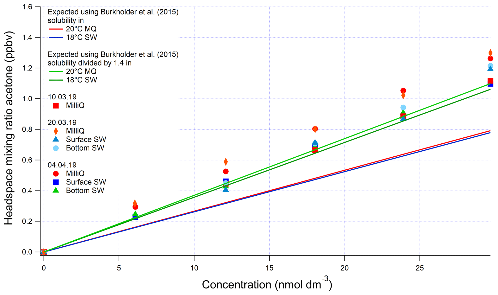
Figure A1 Evasion calibrations using liquid standards of acetone produced by serial dilution in different types of water (SW: seawater; MilliQ: Milli-Q water). Bottom SW refers to seawater collected from well below the mixed layer, near the bottom of the water column. Surface SW refers to seawater collected from the underway seawater inlet. The average measured slope in the four seawater calibrations is 0.0388±0.004 (SD) ppbv (nmol dm⁻³)⁻¹ (10 % rel. SD) and the average slope in the four Milli-Q calibrations is 0.0398±0.002 (SD) ppbv (nmol dm⁻³)⁻¹ (5 % rel. SD). Expected mixing ratios are slightly different between Milli-Q and SW due to the lower seawater temperature.

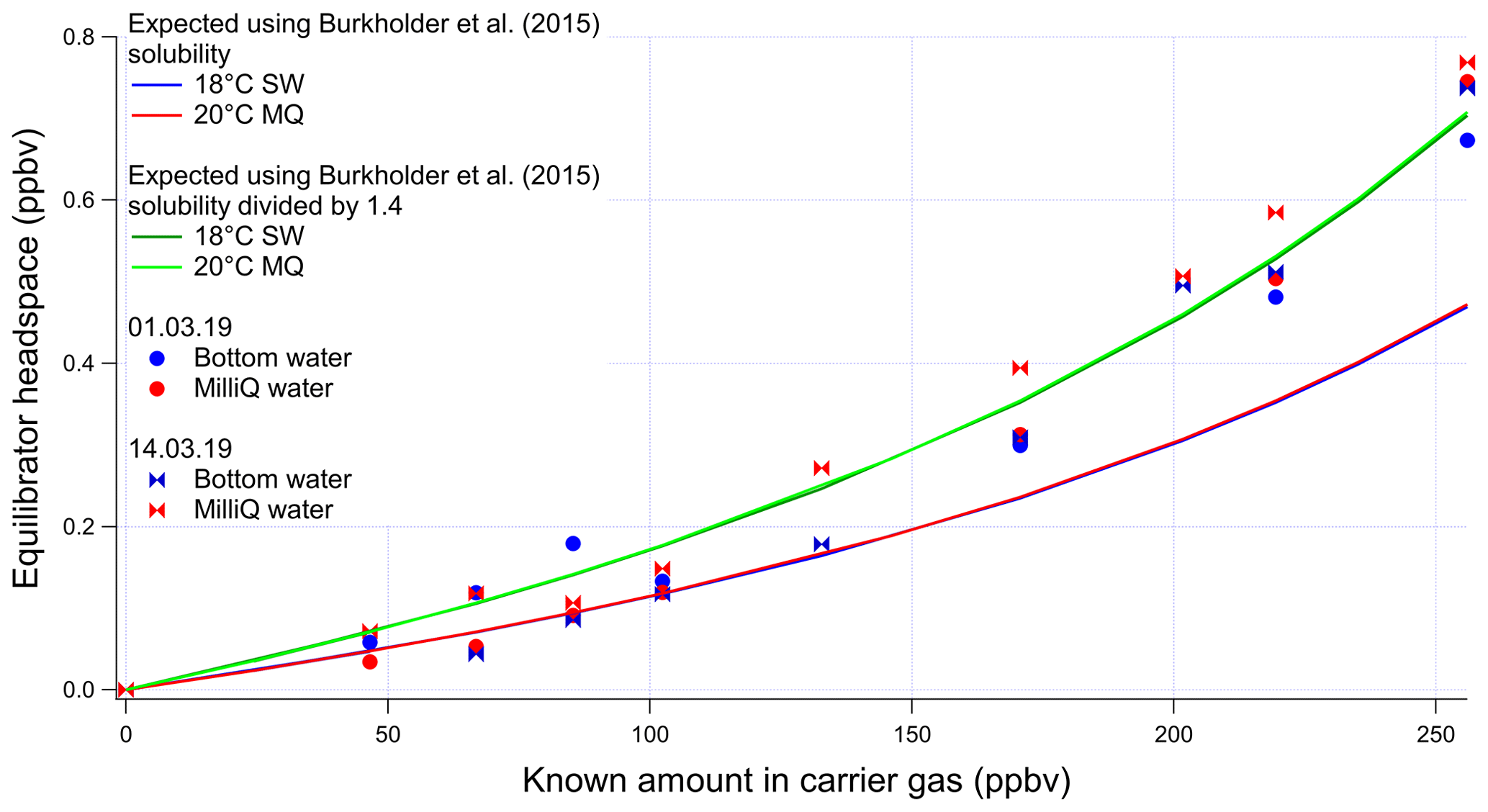
Figure A2 Invasion calibrations for acetone carried out during the deployment and using different types of water (SW: seawater; MQ: Milli-Q water). Bottom SW refers to seawater collected from well below the mixed layer. The non-linear response is due to the changing gas flow as more standard gas is added to the zero-air carrier gas, which alters the purging factor.

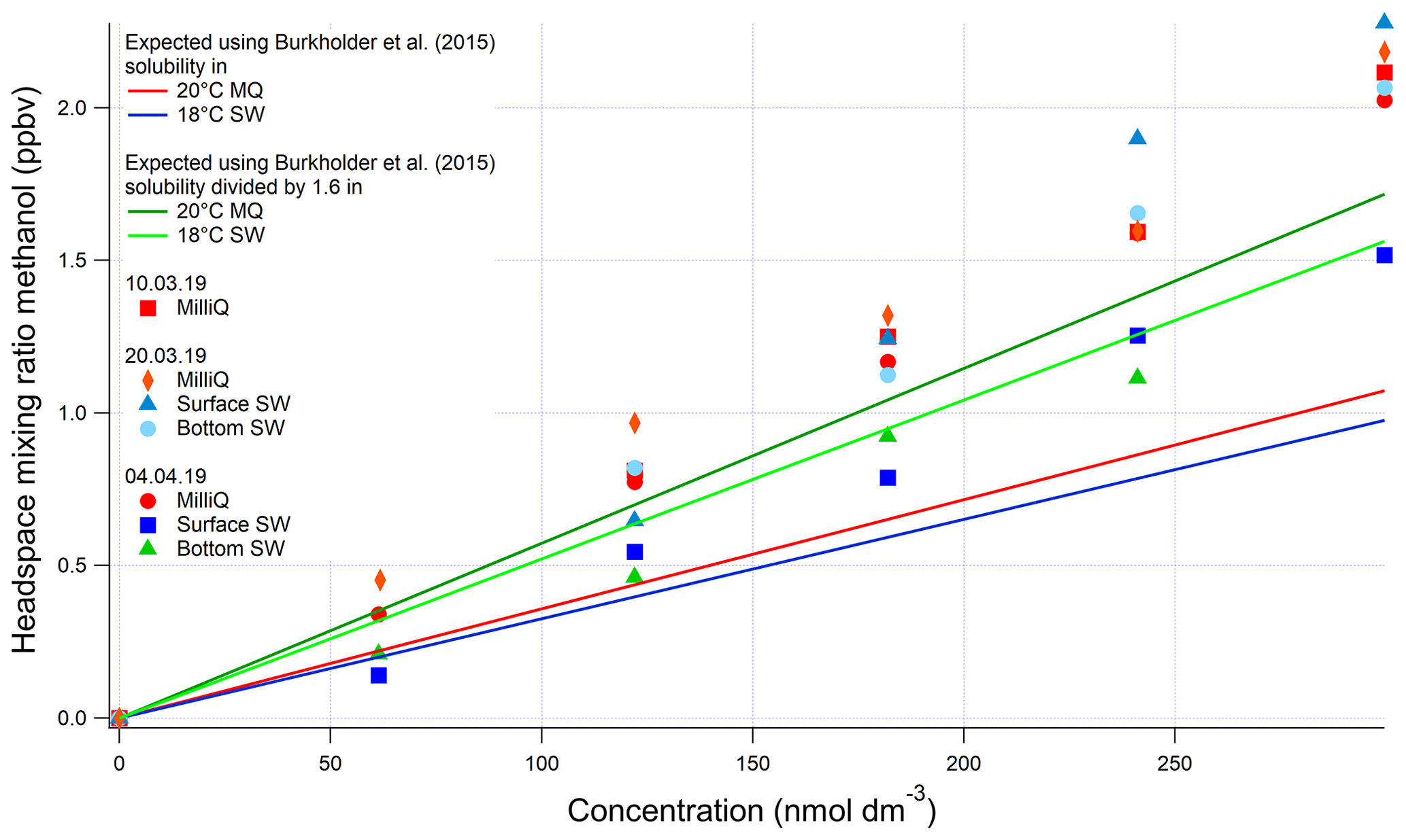
Figure A3 Evasion calibrations using liquid standards of methanol produced by serial dilution in different types of water (SW: seawater; MQ: Milli-Q water). Bottom SW refers to seawater collected from well below the mixed layer. Surface SW refers to seawater collected from the underway seawater inlet. The average measured slope in the four seawater calibrations is 0.00624±0.00121 ppbv (nmol dm⁻³)⁻¹ (19 % rel. SD), and the average slope in the four Milli-Q calibrations is 0.00678±0.000254 ppbv (nmol dm⁻³)⁻¹ (3 % rel. SD). Expected mixing ratios are slightly different between MQ and SW due to the lower seawater temperature.

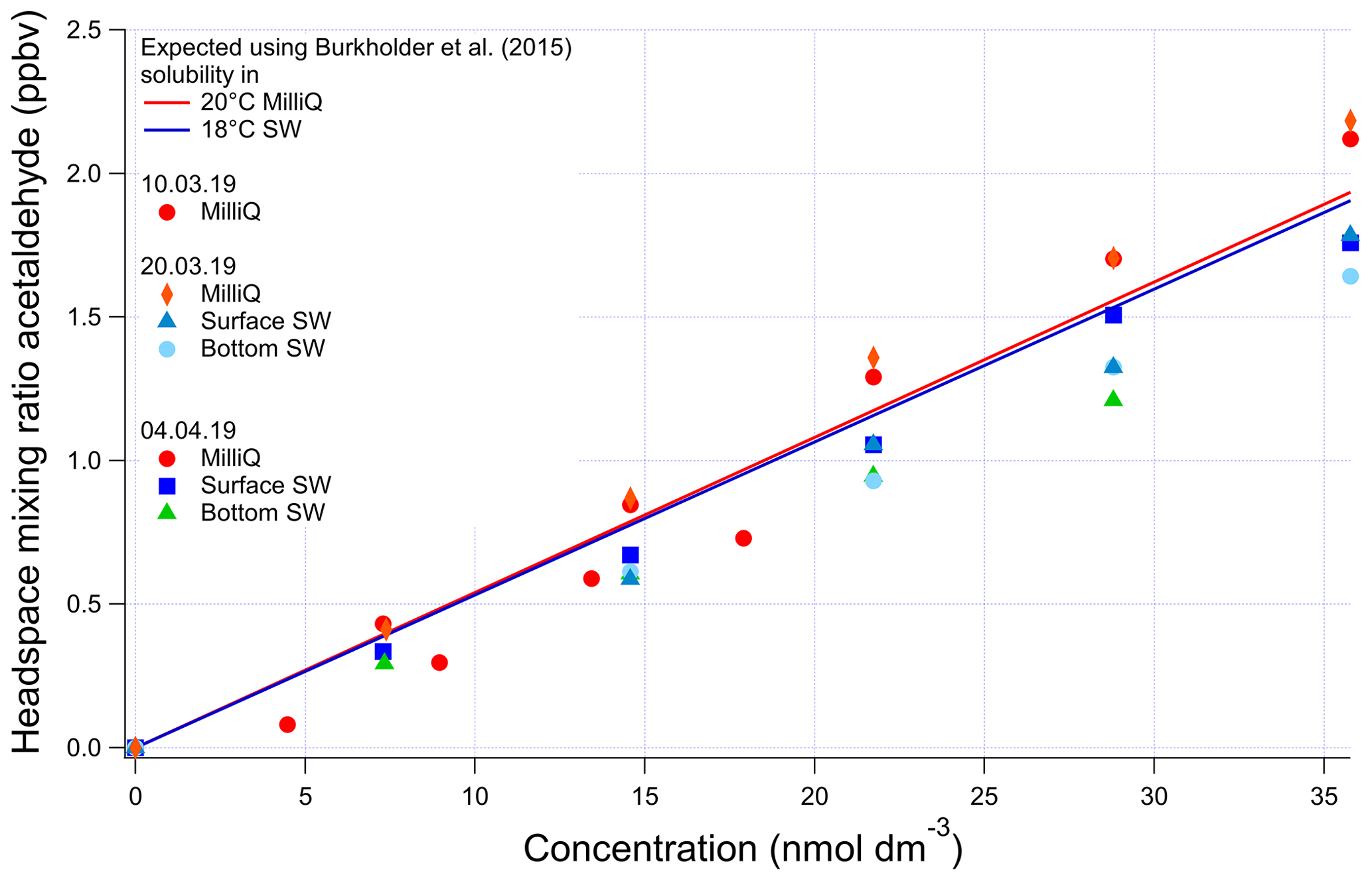
Figure A4 Evasion calibrations using liquid standards of acetaldehyde produced by serial dilution in different types of water (SW: seawater; MilliQ: Milli-Q water). Bottom SW refers to seawater collected from well below the mixed layer. Surface SW refers to seawater collected from the ship's underway seawater inlet. The average measured slope in the four seawater calibrations is 0.0473±0.00313 ppbv (nmol dm⁻³)⁻¹ (6 % rel. SD), and the average slope in the four Milli-Q calibrations is 0.0548±0.00767 ppbv (nmol dm⁻³)⁻¹ (14 % rel. SD). Expected mixing ratios are slightly different between Milli-Q and SW due to the lower seawater temperature.

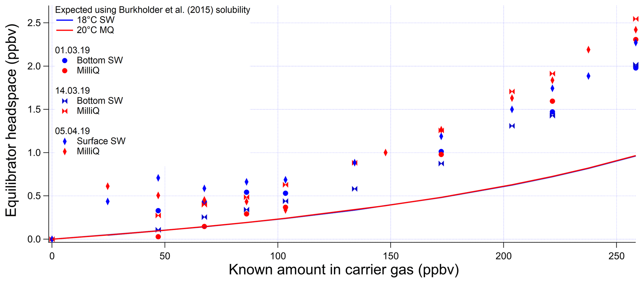
Figure A5 Invasion calibrations for acetaldehyde carried out during the deployment and using different types of water (SW: seawater; MQ: Milli-Q water). Bottom SW refers to seawater collected from well below the mixed layer. Surface SW refers to seawater collected from the ship's underway seawater inlet. The non-linear response is due to the changing gas flow as more standard gas is added to the zero-air carrier gas, which alters the purging factor.