One size fits all? Calibrating an ocean biogeochemistry model for different circulations

Global biogeochemical ocean models are often tuned to match the observed distributions and fluxes of inorganic and organic quantities. This tuning is typically carried out “by hand”. However, this rather subjective approach might not yield the best fit to observations, is closely linked to the circulation employed and is thus influenced by its specific features and even its faults. We here investigate the effect of model tuning, via objective optimisation, of one biogeochemical model of intermediate complexity when simulated in five different offline circulations. For each circulation, three of six model parameters have been adjusted to characteristic features of the respective circulation. The values of these three parameters – namely, the oxygen utilisation of remineralisation, the particle flux parameter and potential nitrogen fixation rate – correlate significantly with deep mixing and ideal age of North Atlantic Deep Water (NADW) and the outcrop area of Antarctic Intermediate Waters (AAIW) and Subantarctic Mode Water (SAMW) in the Southern Ocean. The clear relationship between these parameters and circulation characteristics, which can be easily diagnosed from global models, can provide guidance when tuning global biogeochemistry within any new circulation model. The results from 20 global cross-validation experiments show that parameter sets optimised for a specific circulation can be transferred between similar circulations without losing too much of the model's fit to observed quantities. When compared to model intercomparisons of subjectively tuned, global coupled biogeochemistry–circulation models, each with different circulation and/or biogeochemistry, our results show a much lower range of oxygen inventory, oxygen minimum zone (OMZ) volume and global biogeochemical fluxes. Export production depends to a large extent on the circulation applied, while deep particle flux is mostly determined by the particle flux parameter. Oxygen inventory, OMZ volume, primary production and fixed-nitrogen turnover depend more or less equally on both factors, with OMZ volume showing the highest sensitivity, and residual variability. These results show a beneficial effect of optimisation, even when a biogeochemical model is first optimised in a relatively coarse circulation and then transferred to a different finer-resolution circulation model.

1 Introduction

Global models of marine biogeochemistry are applied to prognostic problems, such as the future exchange of CO₂ between the ocean and atmosphere, the evolution of oxygen minimum zones (OMZs) under a changing climate or future primary production, which is the ultimate food source for fish. Unfortunately, in steady state, these models vary greatly in their representation of, for example, ocean oxygen inventory (up to 50 % of the current value; Bopp et al., 2013) or primary production (varying by more than 90 % of present-day global production; Bopp et al., 2013). The largest uncertainty is related to OMZ volume – here Bopp et al. (2013) report a range of variation that is several times the observed volume, depending on the criterion (maximum oxygen concentration) used for OMZ definition.

Because these coupled models differ in both their physical and biogeochemical setups, to date the contribution of the different model components to this large variation is not clear (e.g. Cabre et al., 2015). Studies indicate a strong impact of physics on deep oxygen levels, leading to a divergence of up to 150 mmol O₂ m⁻³ (Najjar et al., 2007; Séférian et al., 2013). On the other hand, Kriest et al. (2012) and Kriest and Oschlies (2015) showed that the impact of biogeochemical model structure and parameters on deep oxygen profiles can be equally large; also, in the latter study OMZ volume varied among different biogeochemical model setups up to 3 times the observed value (for an OMZ criterion of 8 mmol O₂ m⁻³). Thus, so far neither oxygen content nor OMZ volume seems well constrained, possibly because of both circulation and biogeochemistry.

In practice, biogeochemical models are often tuned to the corresponding circulation, in order to make the model results (nutrients, oxygen, organic components) agree better with observations (e.g. Schwinger et al., 2016). To keep the number of computationally expensive global simulations low, this model calibration is usually carried out “by hand”, i.e. by subjectively tuning some biogeochemical model parameters until the models show a good fit to the observed tracer fields. The criterion for “good” is not absolute – it may consist of a sufficient visual match, good indices of some core statistics (e.g. in Taylor plots;  Taylor, 2001), the root-mean-squared error of model results vs. observed quantities or non-parametric methods such as the Bhattacharyya distance (e.g. Ilyina et al., 2013). Ideally these converge; i.e. they result in a well-defined set of parameters, which provides an optimal fit for all metrics.

However, biogeochemical models include a high-dimensional parameter space with respect to the biogeochemical constants, many of which are not well known. Carrying out a sensitivity study helps to explore a model's sensitivity to its constants (e.g. Kriest et al., 2012), but this is a time-consuming task, in terms of both work hours and computational time. The computational demand is amplified by the fact that global biogeochemical ocean models require a long time to equilibrate (many millennia), owing to the sluggish circulation (e.g. Wunsch and Heimbach, 2008; Primeau and Deleersnijder, 2009) and because biogeochemical processes act in concert with it (e.g. Kriest and Oschlies, 2015). Short spinup times, on the other hand, will produce model results that still depend on initial conditions and can hamper a thorough assessment of model skill. Because of these difficulties, there is no common recipe for model spinup (and calibration). This complicates model inter-comparison (Séférian et al., 2016).

Recently, tools have become available to speed up model equilibration, either by efficient offline methods (Khatiwala, 2007) or by root-finding algorithms that solve for the model's steady state (Li and Primeau, 2008; Khatiwala, 2008). Using these tools, automatic calibration of global biogeochemical ocean models becomes more feasible (e.g. DeVries et al., 2014; Holzer et al., 2014; Letscher et al., 2015; Kriest et al., 2017; Kriest, 2017). However, these approaches have so far mostly been applied to biogeochemical models of low complexity or to circulation models of rather coarse resolution. As physical processes and resolution can play a large role in the representation of biogeochemical tracer distributions (e.g. Najjar et al., 2007; Duteil et al., 2014), it would be desirable to apply optimisation directly to the more highly resolved models applied in prognostic simulations. Yet, to date this approach has proven to be prohibitive, due to the large computational demand mentioned above.

Therefore, we currently must accept a trade-off between finely resolved representation of physical transport processes and well-tested and objectively optimised biogeochemical models. The calibration of model biogeochemistry in one computationally cheap circulation may elucidate the model's behaviour in its (biogeochemical) parameter space and indicate a best set of parameters consistent with observed tracer fields. If the mean transport simulated by models were independent from model resolution, one could then transfer these parameters into the more expensive, high-resolution model. However, like biogeochemical models, physical parameterisations also reflect an idealised system, which can introduce errors in small- and large-scale patterns and processes. Biogeochemical model calibration is affected by these physical errors – the resulting optimal parameters can thus strongly depend on the circulation applied (Löptien and Dietze, 2019). So far it is not clear how model dynamics and performance will change once these calibrated parameters are transferred to a different circulation that resolves physical processes in more detail.

To investigate the mutual effects of circulation, biogeochemical model parameters and model performance, we have tested the effect of five different circulations on the objectively optimised parameters of a biogeochemical model. The ocean models differ in resolution as well as physical forcing and dynamics. Biogeochemical model calibration against nutrients and oxygen was carried out using a quasi-evolutionary algorithm, which carries out a dense scan of a six-dimensional, biogeochemical parameter space. Differences in optimal parameters are discussed before the background of large-scale physical properties. In portability experiments we examine model performance when parameters optimal for one circulation are transferred into another circulation. We finally quantify the effects of changes in parameter sets vs. those of circulation on global quantities such as oxygen inventory, OMZ volume and global biogeochemical fluxes.

2 Models, experiments, and optimisations

2.1 Circulation and physical transport

All model simulations and optimisations apply the transport matrix method (TMM; Khatiwala, 2007, 2018) as an efficient “offline” method for ocean passive tracer transport. The TMM represents advection and mixing in the form of transport matrices that have been calculated from an ocean circulation model simulation prior to the biogeochemical simulations performed here. For our model simulations we apply monthly mean transport matrices (TMs), as well as monthly wind speed, temperature and salinity for air–sea gas exchange. One set of TMs and forcing have been derived from a 2.8^∘ global configuration of the MIT ocean model with 15 vertical levels (Marshall et al., 1997; see also Table 1). Using this rather coarse spatial grid and a time step length of 1∕2 d for tracer transport, a model setup with seven tracers can be integrated for 3000 years in ≈1–1.5 h on four nodes of Intel Xeon Ivybridge at the North-German Supercomputing Alliance (http://www.hlrn.de, last access: 16 June 2020). This circulation is hereafter referred to as MIT28. For the second physical model configuration (hereafter referred to as ECCO), we apply TMs derived from a circulation of the Estimating the Circulation and Climate of the Ocean (ECCO) project, which provides circulation fields that yield a best fit to hydrographic and remote sensing observations over the 10-year period 1992 through 2001 with a horizontal resolution of $\mathrm{1}{}^{\circ }\times \mathrm{1}{}^{\circ }$ and 23 levels in the vertical (Stammer et al., 2004). A full spinup (3000 years) of the coupled model requires about 9 h on 16 nodes of Intel Xeon Ivybridge.

Table 1 General setup, performance and results of optimisations expressed as N, the number of generations (each with a population size of 10) until convergence of the optimisation algorithm, the minimum misfit J^* (the target of optimisation), bias of global average nitrate and oxygen, OMZ volume (for OMZs defined by O₂<50 and O₂<80 mmol m⁻³), optimal parameters, and their uncertainties. To determine parameter uncertainty, we defined the group Ω of model simulations whose misfit J_k deviates less than 1 % from the optimal misfit J^* ($J_k/J^{*}-\mathrm{1}\le \mathrm{0.01}$). For each parameter the first value gives the optimal parameter, averaged over the last generation, and the range of all individuals of Ω is given in square brackets. See Sect. 2.1 for more information on the setup of the offline circulations.

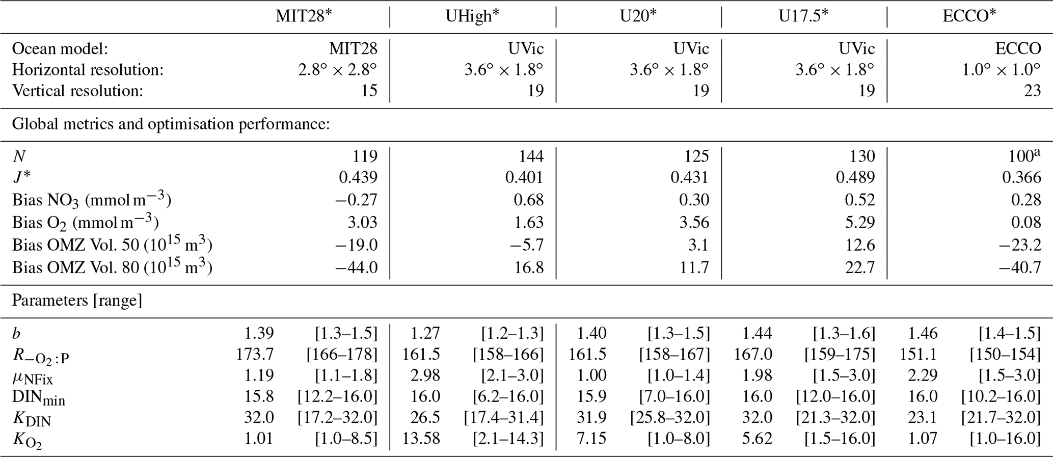
^a Optimisation ECCO^* was stopped at generation 100, when the minimum misfit varied less than 10⁻⁴ around the optimal value.

Finally, three sets of transport matrices have been derived from version 2.9 of the University of Victoria Earth System Climate Model (UVic ESCM, hereafter called “UVic”; Weaver et al., 2001), a coarse-resolution ($\mathrm{1.8}{}^{\circ }\times \mathrm{3.6}{}^{\circ }\times \mathrm{19}$ vertical layers) ocean–atmosphere–biosphere–cryosphere–geosphere model. TM extraction was carried out as described by Kvale et al. (2017). One set of TMs is identical to that described in Kvale et al. (2017) and includes tidal mixing and a high-mixing scheme in the Southern Ocean, as well as an increased low-latitude isopycnal diffusivity (configuration “UHigh”). This configuration utilises a vertical diffusion coefficient of 0.43 cm² s⁻¹ to stabilise meridional overturning in its linear, third-order upwind-biased advection scheme (UW3, Holland et al., 1998; Griffies et al., 2008). This vertical diffusion coefficient is more than double the “standard” value of 0.15 cm² s⁻¹, typically used with the UVic ESCM configured with the default first-order flux-corrected transport (FCT; Weaver and Eby, 1997) advection scheme. Reasons for the change in advection scheme for the application of the TMM to UVic are given in Kvale et al. (2017), but it is important to note here that the UW3 configuration has not benefitted from the more than 2 decades of careful parameter adjustments that users of the FCT configuration appreciate. The annual maximum global meridional overturning strength in the UHigh configuration is 18.5 Sv, but other physical features of the circulation have not been previously assessed in detail. Two further sets of UVic ESCM TMs do not include regional adjustments to mixing. They have been tuned to a maximum annual average global overturning circulation of either 20 Sv (named U20) or 17.5 Sv (named U17.5). This tuning was achieved by adjusting the vertical diffusion coefficient (0.409 cm² s⁻¹ in U17.5 and 0.4179 cm² s⁻¹ in U20). The physical circulation parameterisation is otherwise identical to UHigh: utilising UW3 advection and the same tidal mixing scheme. Differences arising in the calibrations between UVic ESCM TMs therefore reflect differences in both the application of regional mixing “corrections” (UHigh vs. U17.5 and U20) and in global overturning strengths and secondary effects from changed values of the vertical diffusion coefficient. We note that none of the circulation configurations, aside from UHigh, have been previously evaluated against the most commonly used UVic ESCM FCT configuration (e.g. Weaver et al., 2001; Schmittner et al., 2005; Somes et al., 2013).

2.2 Properties of circulation models

The five circulations differ in many aspects. First, being supported by observational data, ECCO's spatial salinity and density distribution agrees very well with observations, while the MIT28 and UVic circulations show, for example, a too shallow depth of the σ=27.5 isopycnal in the Atlantic Ocean and too saline waters in the deep northern North Atlantic (Figs. 1 and S1 in the Supplement). In addition, the three UVic circulations all suffer from a too weak formation and northward propagation of Antarctic Intermediate Waters (AAIW), as identified from water of low salinity at ≈1000 m depth in the Southern Hemisphere. MIT28, U20 and U17.5 also show a too large outcrop area of dense waters (σ_θ≥27.5) in the Southern Ocean, which does not agree with the observed pattern. Here ECCO and UHigh better match observations.

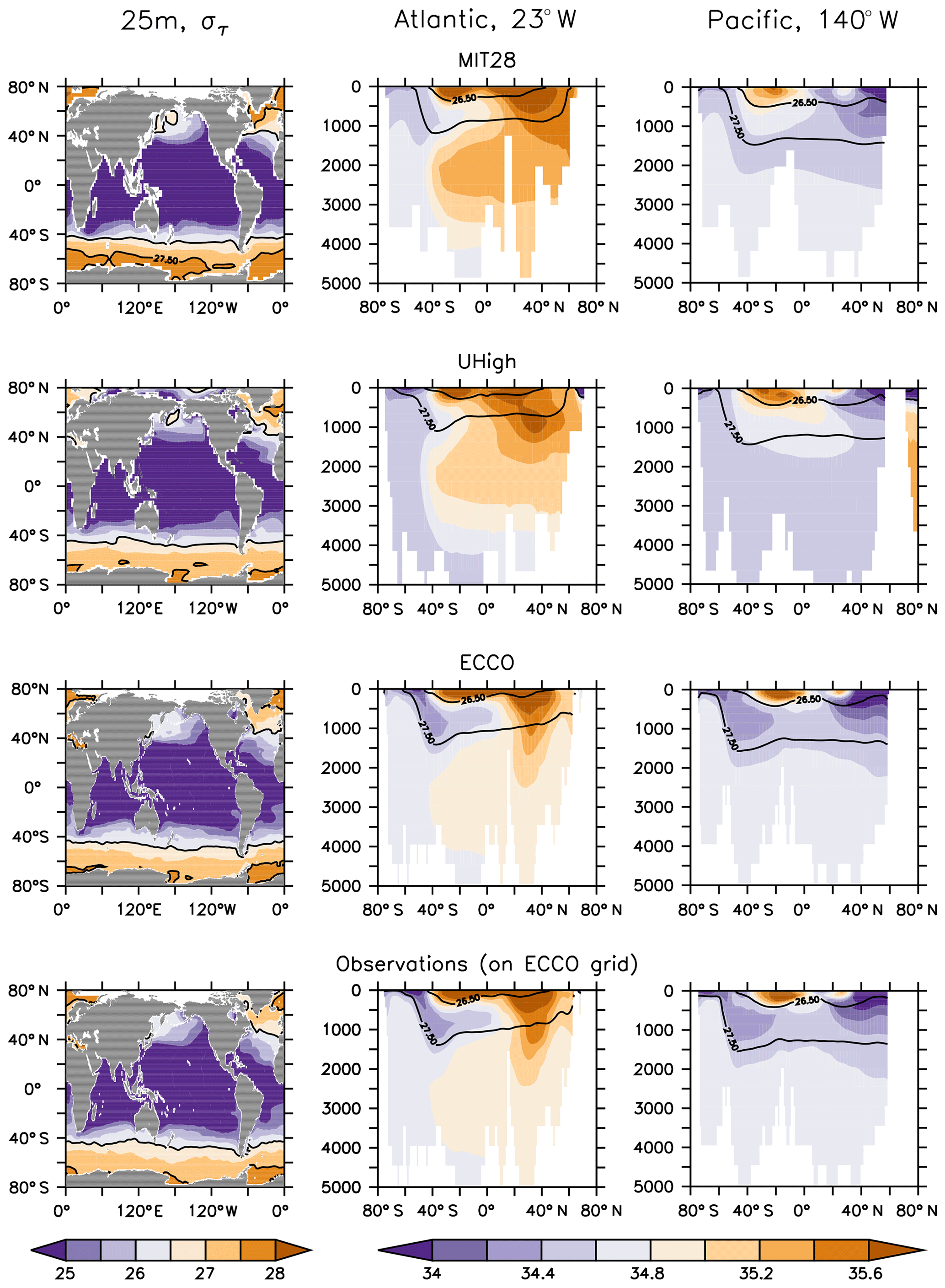
Figure 1 Density (σ_θ) at 25 m (left panels) and salinity along sections at 23 and 140^∘ W (middle and right panels) of forcing from (top to bottom) MIT28, UHigh and ECCO circulation. The bottom row of panels show observations mapped onto ECCO geometry. Density has been derived from annual mean potential temperature and salinity. Contour lines highlight isopycnal of σ_θ=26.5 and σ_θ=27.5.

Figure 2 Annual maximum mixed-layer depths of models and observations (gridded onto ECCO model geometry). Mixed-layer depths have been determined from a density difference of σ_θ=0.03 (density calculated from monthly mean temperature and salinity).

Striking differences also occur with respect to the annual maximum mixed-layer depth, as derived from a potential density difference to the surface of Δσ_θ≥0.03 (Fig. 2), calculated from the models' monthly mean temperature and salinities. Obviously, MIT28 shows a too large area of deep mixing around 60^∘ S in the Southern Ocean, which does not agree with mixed-layer depths derived from observed temperature and salinity. On the other hand, only this circulation exhibits deep mixing in the Labrador Sea, which is in agreement with observations. All configurations of UVic exhibit a too large area of deep mixing in the Southern Ocean, while ECCO tends to underestimate mixing in this area.

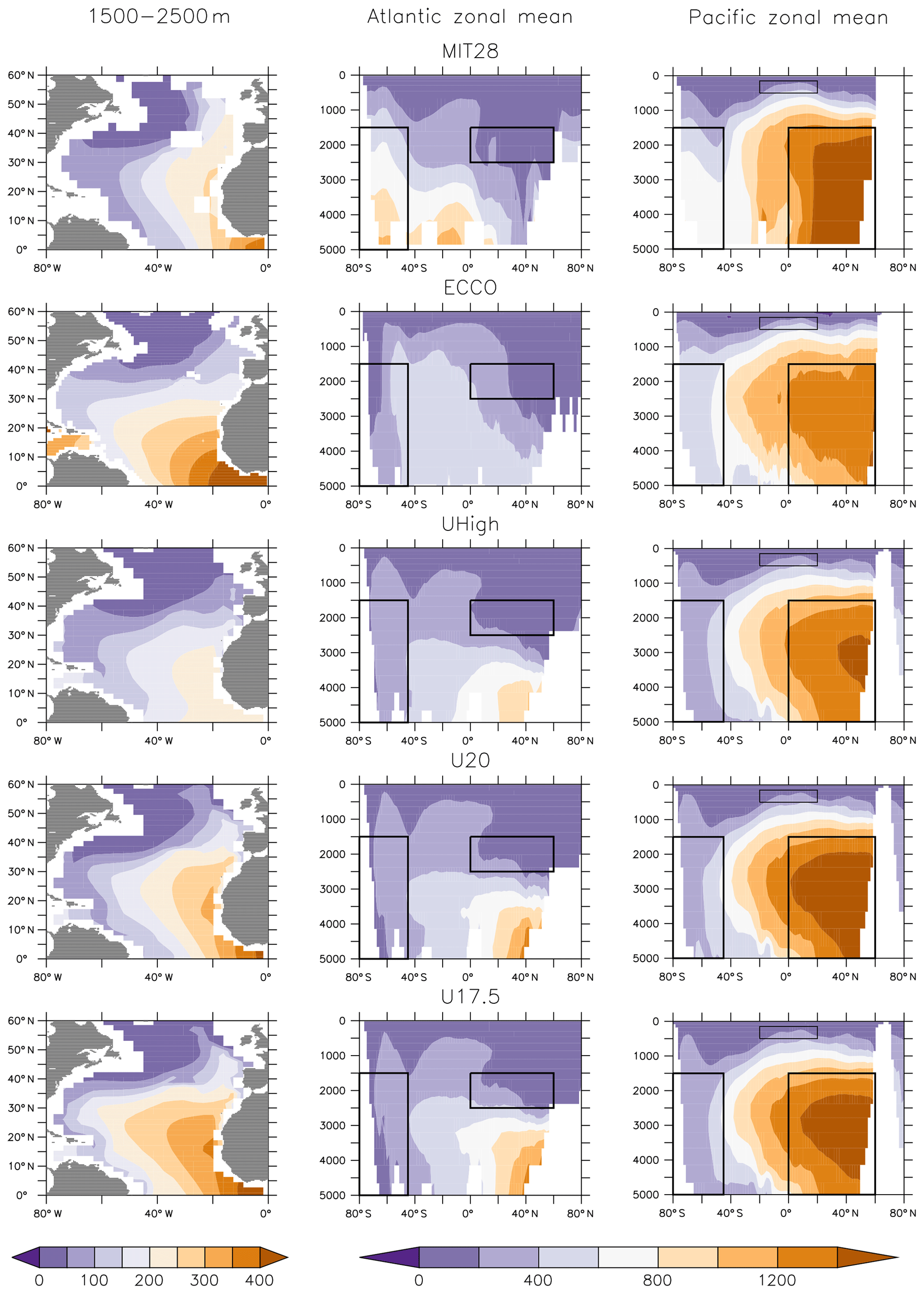
Figure 3 Simulated ideal age (years) averaged over 1500–2500 m in the North Atlantic (NADW, left panels) and as zonal mean for the Atlantic (middle panels) and the Pacific (right panels). Boxes indicate regions of NADW, NPDW, CDW and ETP (see Fig. S2 for detailed plot).

Differences between circulations are also reflected in the global distributions of ages diagnosed from the models. MIT28, U20 and U17.5 show very old (>1400 years) waters in the deep northern North Pacific (Fig. 3). Here, ECCO and UHigh contain much younger waters, mostly below 1400 years. In MIT28 the age increases rapidly with depth in the Southern Ocean (up to more than 800 years). Especially ECCO but also UVic exhibit much younger waters below 2000 m in this region. Finally, the U20 and U17.5 configurations result in too old deep waters in the northern North Atlantic (Khatiwala et al., 2012, their Fig. 4). In general, ECCO and UHigh agree much better with mean age constrained with transient (radiocarbon, chlorofluorocarbons – CFCs) and hydrographic (temperature, salinity, nutrients, oxygen) tracer observations (Khatiwala et al., 2012).

To summarise, our applied offline circulations for MIT28 and ECCO differ strongly with respect to resolution and many global physical properties, with the UVic configurations in between these two. As a data-constrained circulation, ECCO shows the best overall agreement with observations of all five circulations.

2.3 Derived indicators of circulation

The underlying circulation models, from which the TMs and forcing were extracted, differ in many aspects, such as parameterisation of mixing, forcing, sea ice, etc., all of which can affect their dynamic behaviour and the quantities and diagnostics described above. For example, in the Southern Ocean the eastward transport of waters through the Drake Passage can affect the properties and formation of SAMW (e.g. Sallee et al., 2010, 2013), while parameterisation of sea ice in the models might affect the formation and ventilation of Antarctic Bottom Water (AABW) (Dutay et al., 2002), with consequences for water mass age. It is beyond the scope of this paper to compare and discuss the details of the circulation models. Instead, to examine the potential impact of their characteristic features on optimal biogeochemical model parameters (Sect. 3.2), we will focus on three diagnostics that can be easily derived from most circulation models (see Table S1 in the Supplement for simulated and observed values).

2.3.1 Area of deep mixing

Deep mixing in the North Atlantic supplies oxygen to the ocean (Khatiwala et al., 2012). In the Southern Ocean mode and intermediate waters acquire their biogeochemical signatures north of the Antarctic Circumpolar Current (ACC), before being subducted into the interior ocean. These waters then ventilate the thermocline of the subtropics in the Southern Hemisphere (Sallee et al., 2013). However, as also shown in other studies (for example, Sallee et al., 2013, who found a large variability in Southern Ocean mixed-layer depths simulated by 21 ocean circulation models) the circulations applied in our study differ strongly in the extent and location of deep mixing in this region. To account for the potential effects of this variability on optimal parameter choice, we evaluated the area of annual maximum deep mixing in the two regions. Mixed-layer depth was defined by a density difference of Δσ_θ≥0.03 (in line with de Boyer Montégut et al., 2004; Dong et al., 2008; Sallee et al., 2013), calculated from monthly mean potential temperature and salinity. For the Southern Ocean (south of 40^∘ S) and the North Atlantic (north of 40^∘ N) we then calculated the area, where the annual maximum mixed-layer exceeds either 200 or 400 m (the range of mixed-layer depths simulated and observed in the Southern Ocean; Sallee et al., 2013). Altogether, we thus obtain four different indicators for ocean ventilation through deep ocean mixing

2.3.2 Outcrop area of mode and intermediate water masses

On centennial timescales the Antarctic Intermediate Water (AAIW) and Subantarctic Mode Water (SAMW) formed in the Southern Ocean determine nutrient concentrations in subtropical areas. Their nitrate deficit and isotopic composition carry signatures of denitrification and nitrogen fixation (Rafter et al., 2013; Tuerena et al., 2015). Given that the models differ so strongly with respect to the surface density in the Southern Ocean (Fig. 1), we evaluated the outcrop area of waters defined by a density of $\mathrm{26.5}\le {\mathit{\sigma }}_{\mathit{\theta }}<\mathrm{27.5}$ and 27.5≤σ_θ in both the Southern Ocean and the northern North Atlantic (defined as above). In the Southern Ocean the first criterion approximately reflects SAMW and AAIW combined, and the second criterion reflects Circumpolar Deep Water (CDW) (similar to the definitions used by Palter et al., 2010; Iudicone et al., 2011; Rafter et al., 2012, 2013). North Atlantic waters defined by densities of $\mathrm{26.5}\le {\mathit{\sigma }}_{\mathit{\theta }}<\mathrm{27.5}$ and σ_θ≥27.5 coincide mainly with the region between 40 and 60^∘ N and the Greenland Sea, respectively (Fig. 1).

2.3.3 Age of water masses

We use the concept of water mass (or ventilation) age as a diagnostic for the combined effects of ocean circulation, mixing and ventilation on the time elapsed since a water parcel has been isolated from the atmosphere. We distinguish between average ideal age in three different water masses by applying the criteria of Matsumoto et al. (2004). According to their water mass definitions, North Atlantic Deep Water (NADW) comprises all waters in the North Atlantic between 0 and 60^∘ N at 1500–2500 m depth. North Pacific Deep Water (NPDW) is defined for a region between 0^∘ and 60^∘ N at 1500–5000 m depth. Finally, Circumpolar Deep Water (CDW) consists of all waters south of 45^∘ S, for a depth between 1500 and 5000 m (see also Fig. 3). We note that, using these region definitions, the average age of NADW is influenced by waters of the eastern tropical Atlantic (ETA), which are quite old in ECCO circulation (>400 years) and young in UHigh (Fig. 3, left panels). One reason for this could be different rates of overturning, which is between 13 and 14 Sv in ECCO (together with a weak western boundary current; Wunsch and Heimbach, 2006), while the UVic configurations are characterised by higher overturning around 17.5 to 20 Sv. Finally, because the eastern tropical Pacific (ETP) is the main region of fixed-nitrogen loss in the models (Kriest and Oschlies, 2015), but the water age in this region varies strongly among the circulations applied in our study (Fig. S2), we also calculated average age in the eastern equatorial Pacific (ETP) at $\pm \mathrm{20}{}^{\circ }$ latitude, east of 160^∘ W and within 150–500 m depth as a fourth potential indicator.

2.4 The biogeochemical model

For all model simulations we apply the Model of Oceanic Pelagic Stoichiometry (MOPS), which simulates the biogeochemical cycling among phosphate, phytoplankton, zooplankton, dissolved organic phosphorus (DOP) and detritus. The model is described in detail in Kriest and Oschlies (2015), and we here only give a brief overview on model structure, with focus on parameters (and processes) affected by optimisation (see below). All components are calculated in units of millimoles of phosphorus per cubic metre. We assume a constant nitrogen-to-phosphorus ratio of organic matter of 16 [mol N:mol P]. The oxygen demand of aerobic remineralisation is given by $R_{-{\mathrm{O}}_{\mathrm{2}}:\mathrm{P}}$ [mol O₂:mol P], following the stoichiometry by Paulmier et al. (2009). In the model oxygen-dependent aerobic remineralisation of organic matter follows a saturation curve with half-saturation constant $K_{{\mathrm{O}}_{\mathrm{2}}}$ mmol m⁻³. With declining oxygen, denitrification takes over as long as nitrate is available above a defined threshold DIN_min mmol m⁻³. Suboxic remineralisation (denitrification) also follows a saturation curve for the oxidant nitrate, defined by the half-saturation constant for nitrate, K_DIN mmol m⁻³. The model assumes immediate coupling of the different processes involved in nitrate reduction to dinitrogen, following the stoichiometry derived by Paulmier et al. (2009). Loss of fixed nitrogen (through denitrification) is balanced by a temperature-dependent parameterisation of nitrogen fixation, which relaxes the nitrate-to-phosphate ratio to d with a maximum rate μ_NFix $\mathrm{\mu }\mathrm{mol}{\mathrm{m}}^{-\mathrm{3}}{\mathrm{d}}^{-\mathrm{1}}$. Detritus sinks with a vertically increasing sinking speed: w=a z m d⁻¹. With a constant degradation rate r=0.05 d⁻¹, in equilibrium this is equivalent to a depth-dependent particle flux curve, corresponding to a power law: $F\left(z\right)=(z/z_{\mathrm{0}}{)}^{-b}$, with $b=r/a$ (see Kriest and Oschlies, 2008). Depending on the rain rate to the sea floor, a fraction of detritus deposited at the bottom of the deepest vertical box is buried in some hypothetical sediment. Non-buried detritus is resuspended into the deepest box of the water column, where it is treated as regular detritus. The global annual burial of organic phosphorus and nitrogen is resupplied in the next year via river runoff (when simulated with MIT28 or ECCO TMs) or at the ocean surface (TMs derived from UVic). We note that in uncalibrated models (e.g. Kriest and Oschlies, 2015) this creates differences of a few percent in the global inventory of nitrate and oxygen. Differences in the regional distribution of nutrients and oxygen are largely comparable in magnitude to those caused by the numerical sinking scheme of detritus (Kriest and Oschlies, 2011). The effect of this process is subject to further research.

2.5 Optimisation algorithm

Optimisation of n=6 biogeochemical model parameters (see Sect. 2.7 for choice of parameters to be optimised) is carried out using an estimation of distribution algorithm, namely the covariance matrix adaption evolution strategy (CMA-ES;  Hansen and Ostermeier, 2001; Hansen, 2006). The application of this algorithm to the coupled biogeochemistry–TMM framework has been presented in detail in Kriest et al. (2017), and we here only give a brief overview. In each iteration (“generation”) the algorithm defines a population of 10 individuals (biogeochemical parameter vectors of length n), sampled from a multivariate normal distribution in ℝⁿ. Following the simulation of these 10 model setups over 3000 years to near-steady state, after which, for example, global oxygen and nitrate inventory change only by a small amount (see Fig. 2 by Kriest and Oschlies, 2015), the misfit (cost) function (presented in Sect. 2.6) is evaluated, and information of the current as well as previous generations is used to update the probability distribution in ℝⁿ such that the likelihood to sample solutions resulting in a good fit to observations increases. Therefore, the population (the number of model simulations per generation) in CMA-ES is smaller and of lower computational demand than in classical evolutionary algorithms, making the algorithm applicable to this computationally expensive problem. On the other hand, with its quasi-stochastic sampling CMA-ES can still to a certain degree perform well with misfit functions characterised by a rough topography (i.e. many local optima; Kriest et al., 2017; Kriest, 2017).

2.6 Misfit (cost) function

As in Kriest et al. (2017) and Kriest (2017) the standard misfit to observations J is defined as the root-mean-square error (RMSE) between simulated and observed annual mean phosphate, nitrate and oxygen concentrations (Garcia et al., 2006a, b), mapped onto the respective three-dimensional model geometry. Deviations between model and observations are weighted by the volume of each individual grid box, V_i, expressed as the fraction of total ocean volume, V_T. The resulting sum of weighted deviations is then normalised to the global mean concentration of the respective observed tracer.

$$\begin{array}{}\text{(1)}& {\displaystyle }{\displaystyle }{J}_{\text{RMSE}}=\sum _{j=\mathrm{1}}^{\mathrm{3}}J\left(j\right)=\sum _{j=\mathrm{1}}^{\mathrm{3}}{\displaystyle \frac{\mathrm{1}}{{\stackrel{\mathrm{‾}}{o}}_j}}\sqrt{\sum _{i=\mathrm{1}}^N(m_{i,j}-o_{i,j}{)}^{\mathrm{2}}{\displaystyle \frac{V_i}{V_{\mathrm{T}}}}}\end{array}$$

$j=\mathrm{1},\mathrm{2},\mathrm{3}$ indicates the tracer type (phosphate, nitrate, oxygen) and $i=\mathrm{1},\mathrm{\dots },N$ represents the model locations of N model grid boxes. ${\stackrel{\mathrm{‾}}{o}}_j$ is the global average observed concentration of the respective tracer. m_i,j and o_i,j are simulated and observed concentrations, respectively. By weighting each individual misfit with volume, J_RMSE serves as a long-timescale geochemical estimator in contrast to a misfit function focusing on (rather fast) turnover in the surface layer or resolving the seasonal cycle.

2.7 Parameter optimisations and cross-validation experiments

The optimisations presented here are based upon two successive optimisations presented by Kriest et al. (2017) and Kriest (2017). Both studies applied MOPS coupled to TMs derived from MIT28. The cost function, as presented in Eq. (1), was calculated after a spinup of 3000 years, as also used in the present study.

In the first optimisation, Kriest et al. (2017) optimised four parameters related to plankton growth and loss terms, together with b and $R_{-{\mathrm{O}}_{\mathrm{2}}:\mathrm{P}}$. The optimal parameters of this first calibration led to a better agreement of simulated global biogeochemical fluxes to observations of primary and export production, zooplankton grazing, particle flux at 2000 m and organic matter burial at the sea floor (Kriest et al., 2017). In a subsequent optimisation Kriest (2017) kept the four optimal plankton parameters fixed and calibrated four parameters related to remineralisation and nitrogen fixation (namely $K_{{\mathrm{O}}_{\mathrm{2}}}$, K_DIN, DIN_min and μ_NFix described in Sect. 2.4), together with b and $R_{-{\mathrm{O}}_{\mathrm{2}}:\mathrm{P}}$ (see Table 1). This second optimisation by Kriest (2017) led to a better match to independent estimates of pelagic denitrification, without deteriorating the matches to observed primary and export production, zooplankton grazing, particle flux at 2000 m, and organic matter burial at the sea floor. It is hereafter referred to as MIT28^* and serves as the starting point for the four additional optimisations presented in this paper.

In particular, we repeated optimisation MIT28^* against Eq. (1) in circulations ECCO, UHigh, U20 and U17.5 described above. In the following we refer to these four additional optimisations and optimal parameter sets as ECCO^*, UHigh^*, U20^* and U17.5^*. To test the portability of optimised parameters to different physical settings, we then transferred the parameter sets of MIT28^*, ECCO^*, UHigh^*, U20^* and U17.5^* to the other four circulations, again simulating each coupled model for 3000 years. Thus, we present results from 25 different model simulations with five different parameter sets and five different circulations.

3 Results

3.1 Performance of optimised models

When optimised for different circulations the coupled models show similar values of the misfit function J^* (Table 1). The misfit decreases with more realistic circulation and physics (according to the criteria described in Sect. 2.2) and is lowest for ECCO^*. Global mean phosphate profiles are quite similar and vary less then 10 % of the observed concentrations at depths below 500 m (Figs. 4a and S3, black lines). The low variation in phosphate might be explained by the fixed phosphorus inventory of the model. Only at the surface, where nutrient concentrations become low, is relative variation larger. However, despite optimisation some regional mismatches remain: for example, the model when optimised for the three UVic circulations shows a considerable overestimate of deep (>3000 m) phosphate in the Atlantic (Fig. S4). All optimal models further underestimate phosphate in the mesopelagic layer of the northern North Pacific.

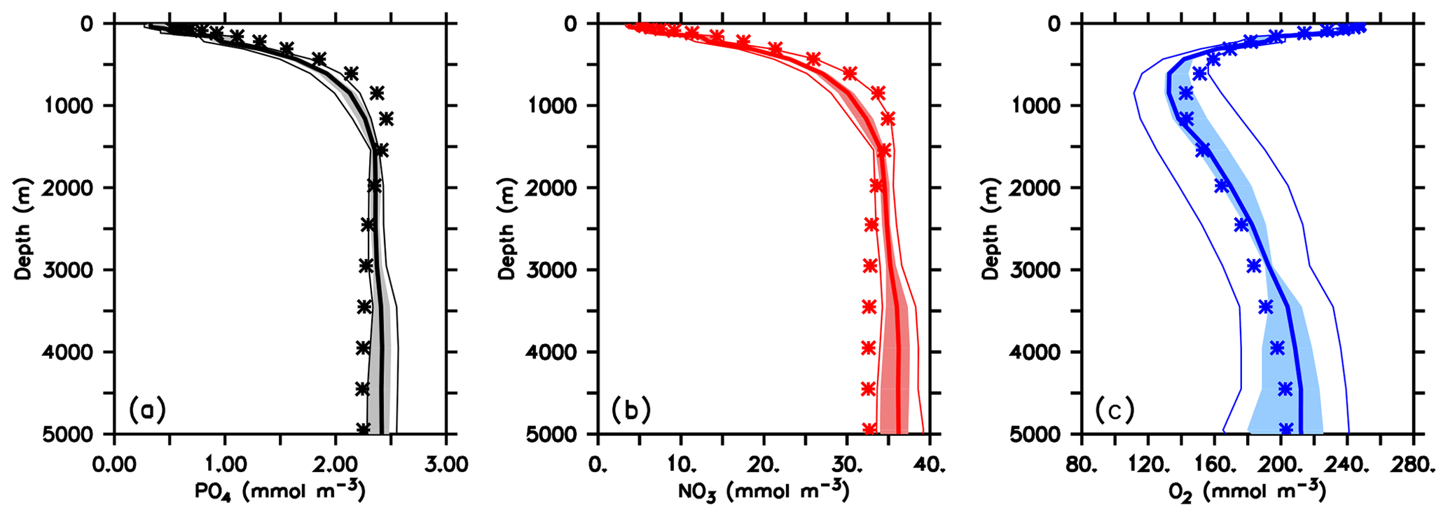
Figure 4 Global mean vertical profiles of phosphate (a), nitrate (b) and oxygen (c). Thin lines denote range across all 25 model experiments, shaded areas the range across the five optimal model experiments and the thick lines the average of optimal model experiments. Stars denote observed profiles. Prior to averaging, all models have been regridded onto the ECCO grid, using nearest-neighbour filling in the vertical and linear interpolation horizontally.

Vertical nitrate profiles are also quite similar to each other (Figs. 4b and S3, red lines), although the nitrate inventory is allowed to adjust dynamically to the loss of fixed nitrogen during denitrification and its balance through nitrogen fixation at the sea surface. Because optimisation also attempts to match nitrate observations, the differences between the models are nevertheless quite small and result in deviations of 1 %–2 % of observed global mean nitrate (see Table 1). The global pattern of nitrate residuals (Fig. S5) generally corresponds to that of phosphate. However, the spatial distribution of fixed-nitrogen gain and loss causes variations in the global distribution of the nitrate deficit in relation to phosphate, as expressed as ${\mathrm{N}}^{*}={\mathrm{NO}}_{\mathrm{3}}-\mathrm{16}\times {\mathrm{PO}}_{\mathrm{4}}$ (Fig. 5).

Figure 5 Excess nitrate N^* (N${}^{*}={\text{NO}}_{\mathrm{3}}-\mathrm{16}\times {\text{PO}}_{\mathrm{4}}$) of optimal model configurations, averaged over the euphotic zone (left panels) and of zonal mean nitrate and phosphate in the Atlantic and Pacific (middle panels and right panels, respectively). Lines denote density of σ_θ=27 and σ_θ=27.5.

In agreement with observations, all optimised models show a large nitrate deficit in the Pacific Ocean, manifest in strongly negative N^* (Fig. 5). This lack of nitrate is caused by denitrification in the ETP and is balanced by nitrogen fixation in the tropics and subtropics (see Fig. S6). In the Atlantic Ocean, where denitrification is largely absent, simulated N^* is far less negative than in other areas, but it is never positive as suggested by the observations. This mismatch can be explained by the prerequisites of the biogeochemical model applied. In MOPS, nitrogen fixation relaxes nitrate to 16× phosphate with a time constant defined by μ_NFix whenever N^* is negative; otherwise it does not occur. Because of this process parameterisation, N^* is restricted to values ≤0. Finally, the Southern Ocean has moderate values of N^*, owing to the mixing of water masses of different origin. Thus, although global average nutrient profiles match observations well, with little differences among optimal models, some regional biases remain, which differ among the models. Also, because of the different processes involved in nutrient turnover, phosphate and nitrate distributions are not exactly the same, with consequences for the nitrate deficit in different oceanic domains.

Global mean oxygen profiles of optimised models vary more strongly than those of nutrients, up to ≈ 40 mmol O₂ m⁻³ in the deep ocean, and thus more than 20 % the observed value (Figs. 4c and S3, blue lines). Overall, a finer resolution and a more realistic circulation improve the representation of this tracer, reducing the global oxygen bias, which ranges from 5.3 mmol O₂ m⁻³ (U17.5^*) to almost zero (ECCO^*; Table 1). On a regional scale all models show some common biases: south of 40^∘ S all optimised models overestimate zonal mean oxygen in subsurface waters above ≈1500 m (MIT28^*) to ≈2000 m (ECCO^*), or even further downward (UVic simulations; Fig. S7). In the Pacific Ocean these too high oxygen concentrations propagate northward. Finally, in mesopelagic waters of the northern North Pacific all models overestimate oxygen, especially above 1000 m. Common to all models is further an underestimate of oxygen in subsurface waters (down to ≈1000 m) in the subtropics and tropics of the Southern Hemisphere. The Atlantic Ocean is generally characterised by too low oxygen concentrations at greater depths. Here, the five optimal models differ: ECCO^* exhibits too low mesopelagic oxygen in the tropical and subtropical Atlantic. MIT28^* underestimates oxygen in particular in deep waters of the Southern Hemisphere and north of 60^∘ N. The optimal UVic configurations are biased low in deep waters of the Northern Hemisphere. These low oxygen concentrations of the UVic configurations are accompanied by too high phosphate and nitrate in the deep North Atlantic (Fig. S5) and indicate too high remineralisation of organic matter in these depths. Together with circulation, this too high remineralisation results in a too strong accumulated signal of remineralisation.

Thus, while there are common features among the five optimal models, there are also some striking differences, especially in the Atlantic. These differences can be explained by the large impact of the Pacific on the misfit function. Owing to its large volume, and the comparatively large impact of oxygen on the misfit function (see Kriest et al., 2017), optimisation will attempt to minimise in particular oxygen misfits in this region and tune the biogeochemical model parameters to compensate for potential errors of the respective circulation. These different parameters affect the oxygen distribution in the Atlantic, which does not contribute so much to the global misfit. Different physical properties of the circulations then cause divergent patterns in the oxygen distribution of this region.

3.2 Best parameters of optimisations in different circulations differ

As presented and discussed by Kriest (2017), optimisation of MOPS in the circulation of MIT28 reduces the particle flux length scale by increasing b from a “default” value of ≈1.1 (Kriest and Oschlies, 2015) to 1.39. It further results in a high nitrate threshold for the onset of denitrification (DIN_min=15.8 mmol m⁻³, compared to the default value of 4 mmol m⁻³ applied by Kriest and Oschlies, 2015), a low affinity of denitrification to nitrate (K_DIN=32 mmol m⁻³) and a low maximum nitrogen fixation rate (${\mathit{\mu }}_{\text{NFix}}=\mathrm{1.19}\mathrm{\mu }\mathrm{mol}{\mathrm{m}}^{-\mathrm{3}}{\mathrm{d}}^{-\mathrm{1}}$; Table 1), which is only about half of the default value applied by Kriest and Oschlies (2015). The optimised oxygen affinity of remineralisation is very high, as indicated by a low value of $K_{{\mathrm{O}}_{\mathrm{2}}}$ (the half-saturation constant for oxygen). We note that $K_{{\mathrm{O}}_{\mathrm{2}}}$ also regulates the inhibition of denitrification by oxygen; when this parameter becomes very low, denitrification is more strongly inhibited by oxygen. Hence, the optimal model configuration MIT28^* induces only moderate denitrification and prevents a decline of the global nitrate inventory through this process (see also Kriest and Oschlies, 2015). The oxygen demand of remineralisation, $R_{-{\mathrm{O}}_{\mathrm{2}}:\mathrm{P}}$, remains close to the value derived from observations (170±10 mmol O₂:mmol P; Anderson and Sarmiento, 1994). Finally, as noted by Kriest (2017), some parameters are only weakly constrained by the misfit function: for example, an almost 10-fold increase in $K_{{\mathrm{O}}_{\mathrm{2}}}$ results in a misfit function not larger than 1 % of the optimal misfit (see also Table 1). One reason for this low sensitivity of the misfit to a variation in $K_{{\mathrm{O}}_{\mathrm{2}}}$, K_DIN or DIN_min is the small volume occupied by suboxic zones, where these parameters can play a role in dissolved inorganic tracer concentrations (Kriest, 2017).

Optimising the same set of parameters in either the three different UVic circulations or the ECCO circulation also results in a high threshold for the onset of denitrification, DIN_min (Table 1). As for MIT28^* the dependencies of oxic and suboxic remineralisation on oxygen or nitrate, expressed through $K_{{\mathrm{O}}_{\mathrm{2}}}$ and K_DIN, may vary largely within the parameter space without having a large impact on the misfit function.

In contrast, $R_{-{\mathrm{O}}_{\mathrm{2}}:\mathrm{P}}$ and b are constrained very well by the misfit function, as indicated by the narrow range of parameters that result in a good fit to observations. For example, all solutions of the ECCO^*, which result in a misfit within 1 % of the optimal fit, require a b value between 1.4 and 1.5 and a stoichiometric demand for oxygen between 150 and 154 mol O₂:mol P (Table 1). Optimal $R_{-{\mathrm{O}}_{\mathrm{2}}:\mathrm{P}}$ decreases from 170 mol O₂:mol P (MIT28^*) over 162 mol O₂:mol P (UHigh^*) to 151 mol O₂:mol P (ECCO^*). The exponent determining the shape of the particle flux curve, b, also varies among the five optimisations, between 1.27 (UHigh^*) and 1.46 (ECCO^*). The range of good (within 1 % of the optimal fit) values for b differs between ECCO^* and UHigh^* (b between 1.2 and 1.3). Also, the range for good values for $R_{-{\mathrm{O}}_{\mathrm{2}}:\mathrm{P}}$ of ECCO^* does not overlap with that of the other optimisations.

Optimal μ_NFix also varies considerably among the different optimisations, from 1 to 3 $\mathrm{\mu }\mathrm{mol}{\mathrm{m}}^{-\mathrm{3}}{\mathrm{d}}^{-\mathrm{1}}$. Here, the range of good parameter values for U20^* (1.0–1.4 $\mathrm{\mu }\mathrm{mol}{\mathrm{m}}^{-\mathrm{3}}{\mathrm{d}}^{-\mathrm{1}}$) does not overlap with that of ECCO^*, UHigh^* and U17.5^* (all between 1.5 and 3 $\mathrm{\mu }\mathrm{mol}{\mathrm{m}}^{-\mathrm{3}}{\mathrm{d}}^{-\mathrm{1}}$). Overall, MIT28^* and U20^* benefit from a low maximum nitrogen fixation rate around 1 $\mathrm{\mu }\mathrm{mol}{\mathrm{m}}^{-\mathrm{3}}{\mathrm{d}}^{-\mathrm{1}}$, while the other models require a larger rate between 2 and 3 $\mathrm{\mu }\mathrm{mol}{\mathrm{m}}^{-\mathrm{3}}{\mathrm{d}}^{-\mathrm{1}}$.

Therefore, to achieve a good fit to observations, different circulations seem to require markedly different parameters for the oxygen utilisation by remineralisation, ($R_{-{\mathrm{O}}_{\mathrm{2}}:\mathrm{P}}$), the exponent determining the particle flux curve (b) and the potential rate of nitrogen fixation (μ_NFix). Other parameters vary little (DIN_min), or (as indicated by overlapping ranges of good parameters) the differences among them might not be relevant ($K_{{\mathrm{O}}_{\mathrm{2}}}$ and K_DIN) for a misfit function targeting the global scale. It is important to note that the relevant parameters do not seem to be correlated with each other (Fig. S8). Apparently, different characteristics of each circulation influence the choice of the optimisation algorithm for the optimal values of $R_{-{\mathrm{O}}_{\mathrm{2}}:\mathrm{P}}$, b and μ_NFix.

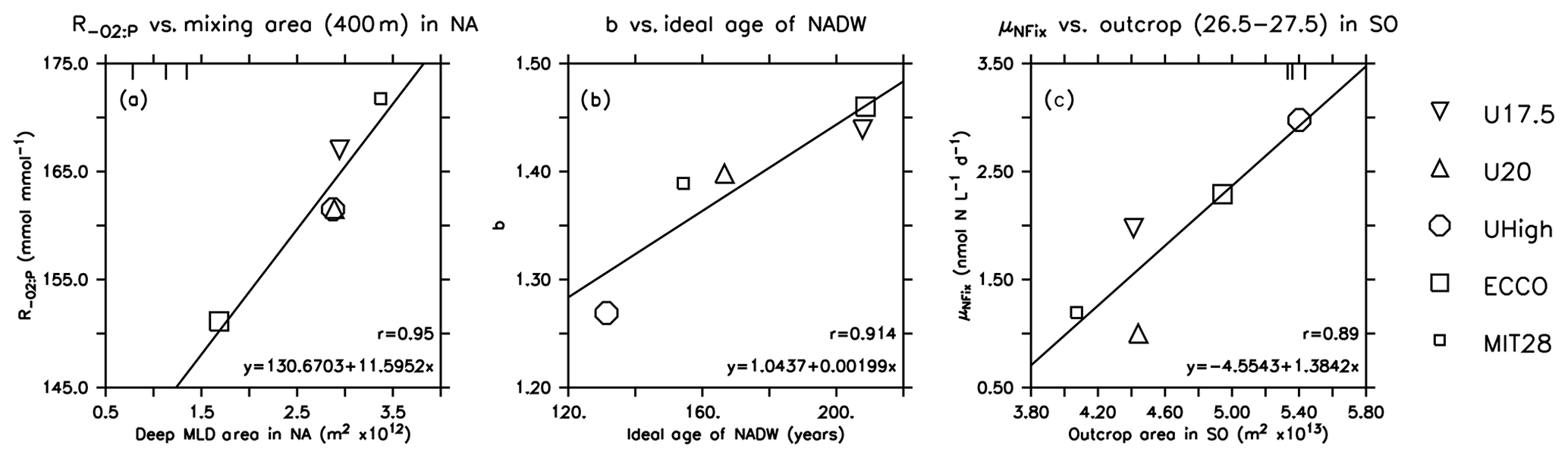
Figure 6 Optimal parameters for which the correlation of Table 2 is significant at p<0.05, plotted against physical diagnostics. Symbols indicate the different model optimisations. Small squares: MIT28^*. Large squares: ECCO^*. Circles: UHigh^*. Triangles: U20^*. Inverted triangles: U17.5^*. Lines denote the regression of optimal parameters against the respective circulation diagnostic. Vertical bars at the upper plot boundary indicate observed diagnostics.

Table 2 Correlation coefficient r for the regression of three optimal model parameters against physical diagnostics. The outcrop area of dense waters in the Northern Hemisphere (>40^∘ N) and Southern Hemisphere (>40^∘ S) is given for two different density intervals. Outcrop area for deep mixing in the North Atlantic (>40^∘ N) and Southern Ocean (>40^∘ S) is given for two different criteria of maximum deep mixing (200 and 400 m). Mean water mass age is given for four different water masses. See text for further details. Significant correlations (p<0.05) are denoted in bold.

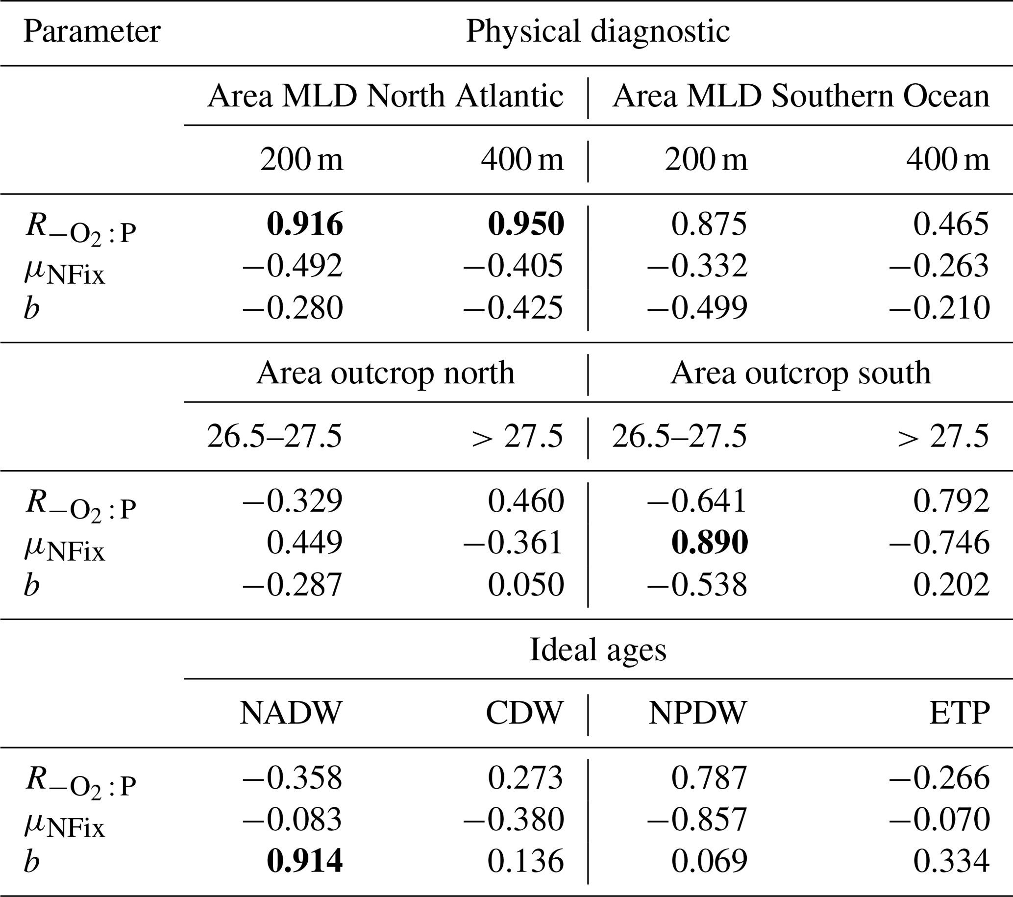
To investigate the potential dependence of optimal parameters on circulation, we examined the area of dense-water outcrop and deep mixing in two different regions (see Sect. 2.3 for definition). Together with average age of four different regions or water masses, we investigate 12 different diagnostics for each circulation for their influence on optimal biogeochemical parameter estimates. In most cases the optimal parameters are not correlated with physical properties (Table 2). However, the oxygen demand of remineralisation, $R_{-{\mathrm{O}}_{\mathrm{2}}:\mathrm{P}}$, is significantly correlated with the area of deep mixing in the northern North Atlantic for maximum mixed-layer depths of 200 and 400 m (p<0.05). For both criteria $R_{-{\mathrm{O}}_{\mathrm{2}}:\mathrm{P}}$ increases with increasing area of deep mixing (Fig. 6). In addition, $R_{-{\mathrm{O}}_{\mathrm{2}}:\mathrm{P}}$ also correlates with a deep mixing area defined by >200 m in the Southern Ocean, albeit not significantly (Table 2). In other words, more vigorous mixing in areas of deep, intermediate or mode water formation allows for a higher oxygen utilisation by remineralisation. Parameter b describing the particle flux curve correlates significantly with the ideal age of NADW (Table 2) and increases with increasing age of this water mass (Fig. 6). Finally, the maximum potential rate of nitrogen fixation μ_NFix correlates with the outcrop area of waters with moderate density ($\mathrm{26.5}\le {\mathit{\sigma }}_{\mathit{\theta }}<\mathrm{27.5}$) waters in the Southern Ocean. An increase in the outcrop area of these waters – which correspond roughly to the sum of AAIW and SAMW – results in an increase in optimal maximum nitrogen fixation rate (Fig. 6). The age of mesopelagic waters in the ETP seems to play a small role, despite the fact that it is an important area in the global nitrogen budget (Fig. S6). Possible reasons for the dependence of these three parameters on physical diagnostics will be discussed in Sect. 4.1.

3.3 Cross-validation experiments: can we transfer parameters optimal for one circulation to another circulation?

Given that three optimal parameters differ among the model circulations, we investigate model performance and dynamics when these parameter sets are swapped among circulations. Of course, every coupled model performs best (with respect to J^* of Eq. 1) when simulated with parameters optimal for the respective circulation, as indicated by the lowest relative misfit along the main diagonal in panel (a) of Fig. 7. When exchanging the biogeochemical parameters optimal for ECCO or MIT28 circulation with parameters optimised in any other circulation, the model performance with respect to J^* deteriorates. The misfit function changes less when the optimal parameters are swapped among the different UVic circulations.

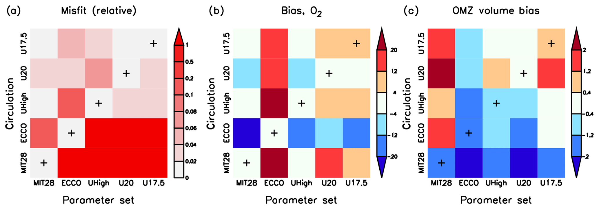
Figure 7 Three different model diagnostics for all cross-validation experiments with parameter set i and circulation j: (a) normalised misfit $J_{i,j}/J_j^{*}-\mathrm{1}$, where $J_j^{*}$ is the lowest misfit for each circulation j. (b) Oxygen bias (model minus observation, mmol m⁻³). (c) OMZ volume (as percent of total ocean volume) bias. OMZs are defined by 50 mmol m⁻³. The x axis denotes the optimal parameter sets of MIT28^*, ECCO^*, UHigh^*, U20^* and U17.5^* and the y axis the circulation. Pluses along the main diagonal indicate the optimal model simulation for each circulation (i=j), i.e. MIT28^*, ECCO^*, UHigh^*, U20^* and U17.5^*.

In the model the global oxygen inventory adjusts dynamically to the combined effects of circulation and biogeochemical parameters, causing a large impact of this tracer on the misfit function (Kriest et al., 2017). Therefore, optimisation attempts to reduce the global oxygen bias, which is low for each optimal model configuration, indicated by the low values along the main diagonal of Fig. 7b. The oxygen bias induced by the changes in parameter set and circulation depends on the combination of these two. For example, the low value for $R_{-{\mathrm{O}}_{\mathrm{2}}:\mathrm{P}}$ and the high value for b of ECCO^* causes a large overestimate of the oxygen inventory in any other circulation (indicated by warm colours in the second column of Fig. 7b). Vice versa, applying optimal parameter sets from MIT28^*, UHigh^*, U20^* or U17.5^* to the ECCO circulation results in a too low oxygen inventory (indicated by cold colours in the second row from the bottom of Fig. 7b). When swapping parameter sets among the different configurations of the UVic circulation, the effect is much less pronounced. Apparently, despite their different overturning and mixing, the UVic circulations are more similar to each other than those of MIT28 and ECCO. We note that these large differences in oxygen inventory arise mainly from deeper (27.5≤σ_θ) layers, while the oxygen inventories of waters lighter than σ_θ=27.5 are quite similar (Fig. S9).

OMZ volume is biased low for the parameter set of ECCO^* and in the MIT28 circulation (Fig. 7c). This underestimate is likely caused by the very low $R_{-{\mathrm{O}}_{\mathrm{2}}:\mathrm{P}}$ and high b of ECCO^*, or the vigorous mixing in the MIT28 circulation, which both tend to increase subsurface oxygen concentrations. Otherwise, OMZ volume does not seem to be closely related to the parameter set or circulation, likely because this diagnostic is largely independent of the applied misfit function and depends on the local circulation pattern (see discussion by Sauerland et al., 2019).

Thus, because of different physical model properties, the biogeochemical model MOPS, when coupled to the MIT28 and ECCO circulation, requires unique and different sets of parameters for optimal model performance. In the UVic circulations the model is more flexible with regard to parameters; yet, when aiming for independent diagnostics such as OMZ volume, there is no clear relationship between OMZ volume and changes in parameter set or circulation.

3.4 Effect of parameters and circulation on phosphate and oxygen concentrations in different water masses

Because of the regional biases of nutrients and oxygen in the North Atlantic, North Pacific and Southern Ocean (see Sect. 3.1), and because the values of $R_{-{\mathrm{O}}_{\mathrm{2}}:\mathrm{P}}$ and b selected in the calibration process correlate significantly on water mass properties of the NADW, NPDW and CDW (Sect. 3.2), we here examine more closely how these parameters affect the large-scale distribution of phosphate (as a conserved nutrient) and oxygen, which can adjust dynamically at the model's air–sea interface and is thus a non-conservative tracer.

Kriest et al. (2012) showed that b, the parameter determining the particle flux length scale, has a large influence on the distribution of phosphate along the “conveyor belt” (i.e. along waters of different age), in agreement with the results obtained by Bacastow and Maier-Reimer (1991) and Kwon and Primeau (2006). We here carry out an analysis similar to that by Kriest et al. (2012) and evaluate average phosphate and oxygen within the NADW, NPDW and CDW, with region definitions as described above for water mass age (Sect. 2.3).

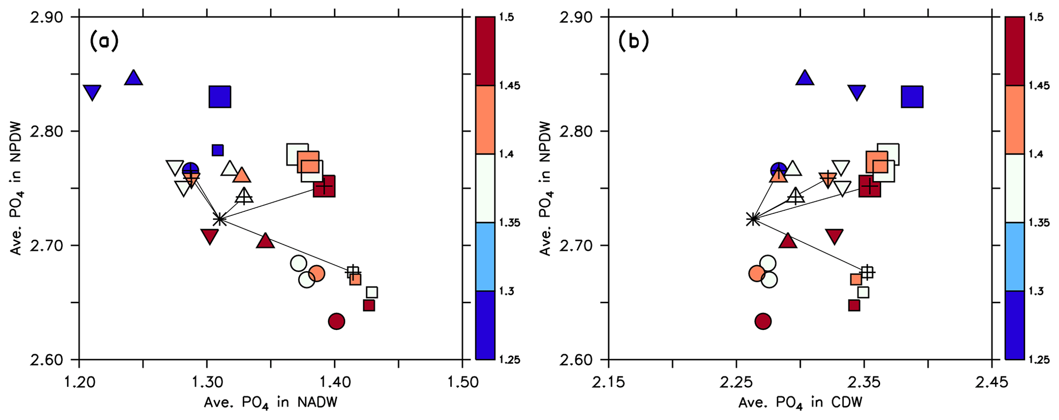
Figure 8 Average phosphate in the northern North Pacific Deep Water (NPDW; between 0 and 60^∘ N at 1500–5000 m; see Sect. 2.3) plotted against average phosphate in the northern North Atlantic Deep Water (NADW; between 0 and 60^∘ N at 1500–2500 m; a) or Circumpolar Deep Water (CDW; south of 45^∘ S, 1500–5000 m; b), of all 25 model experiments. Small squares: MIT28 circulation. Large squares: ECCO circulation. Circles: UHigh circulation. Triangles: U20 circulation. Inverted triangles: U17.5 circulation. (See also symbol legend in Fig. 6.) The colour indicates the value of parameter b. Pluses indicate the optimal parameter set. Stars indicate observed values. Thin black lines extending from the stars denote the distance between observation and each optimal model configuration.

Within each circulation a smaller value of b (corresponding to faster sinking particles) increases phosphate in the NPDW and decreases it in the NADW (Fig. 8a), confirming the pattern found by Kriest et al. (2012). When plotting average phosphate in the NPDW against average phosphate in the CDW, there is no such relationship, but the average value in the CDW varies only little (Fig. 8b) and is near the observed value of 2.26 mmol m⁻³. The spread of phosphate concentrations caused by different parameter sets (same symbol with different colours) is about the same (between 0.1 and 0.15 mmol m⁻³) as the spread caused by different circulations (different symbols of the same colour). Thus, both biogeochemistry and circulation seem to play an equally large role in the distribution of phosphate between NADW and NPDW. The variation caused by biogeochemical parameters is smaller for CDW, indicating that in this region physical processes play a larger role.

Figure 9 As Fig. 8, but for average oxygen and parameter $R_{-{\mathrm{O}}_{\mathrm{2}}:\mathrm{P}}$ (colour scale).

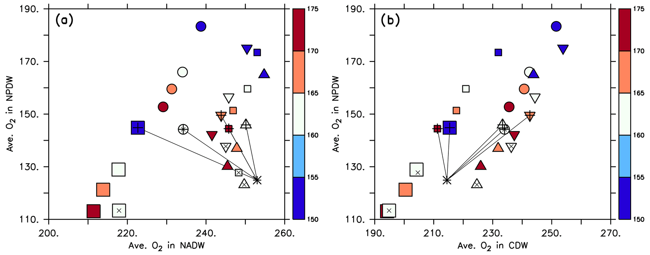
In contrast to phosphorus, the oxygen inventory is not fixed but regulated by the interplay of circulation, air–sea gas exchange and biogeochemical turnover. Because of this we find a pattern that is very different from that of phosphate when examining the distribution of average oxygen in different water masses. Now, within each circulation average oxygen in the NPDW increases almost linearly with average oxygen in the CDW and NADW (Fig. 9), highlighting the role of these waters in the ventilation of the deep North Pacific. In most circulations, a large value of $R_{-{\mathrm{O}}_{\mathrm{2}}:\mathrm{P}}$ results in a low oxygen content in all water masses. All optimised coupled model configurations suggest average oxygen between 220 and 250 mmol m⁻³ in the NADW. For the NPDW all optimised models simulate average oxygen concentrations around 150 mmol m⁻³ and thereby overestimate the observed value of 125 mmol m⁻³ by one-fifth. Average oxygen in the CDW of optimal model simulations varies between ≈210 and 240 mmol m⁻³, encompassing the observed value of 215 mmol m⁻³. Thus, given the quite wide range of potential parameter values, optimisation improves the global oxygen bias (see Table 1), but some residual regional bias in particular in the NPDW remains.

3.5 Effect of parameters and circulation on global oxygen inventory and OMZ volume

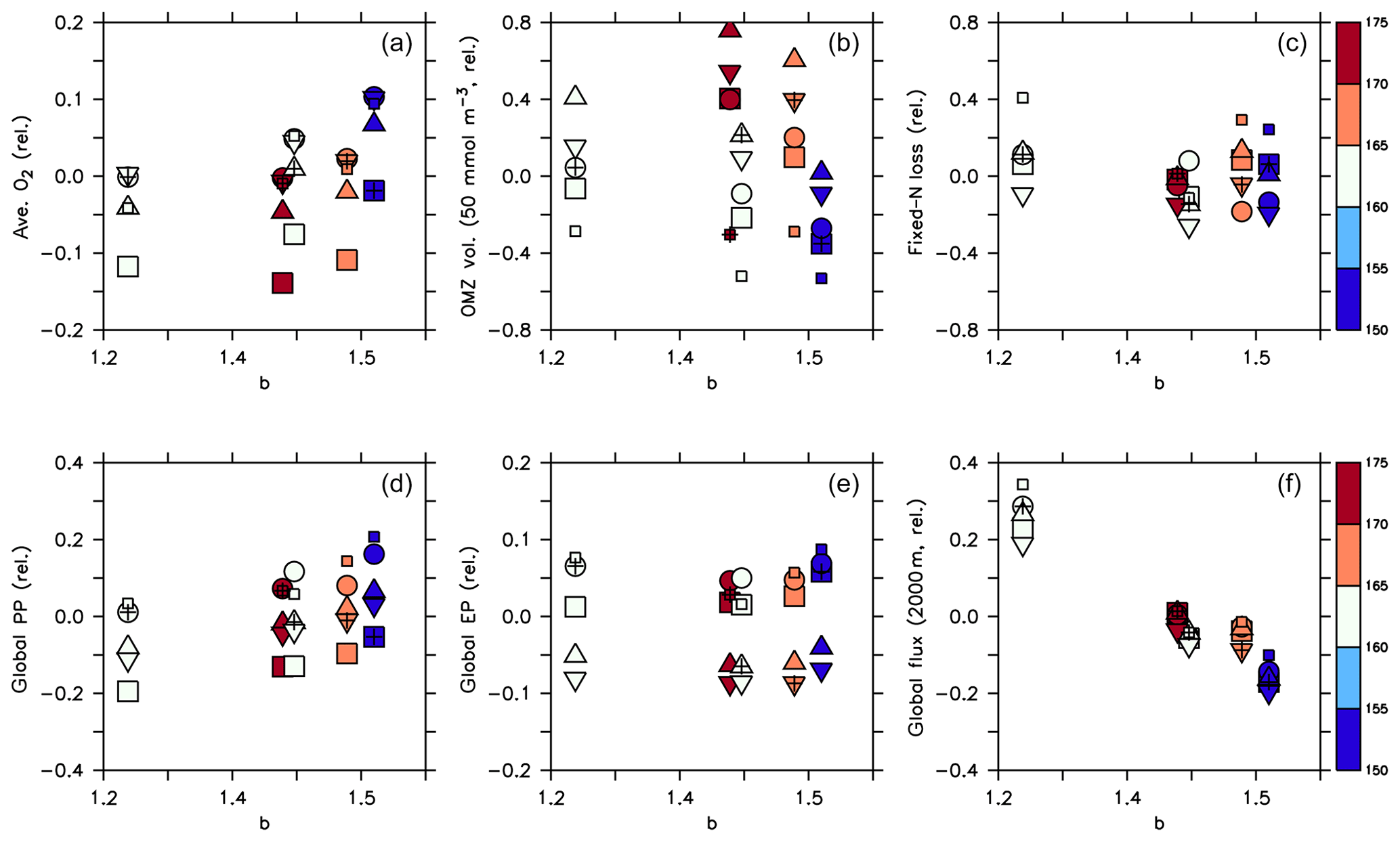
Figure 10 Normalised biogeochemical diagnostics plotted against parameter b: (a) global average oxygen, (b) OMZ volume defined by concentrations <50 mmol m⁻³, (c) global fixed N loss, (d) global primary production, (e) export production and (f) organic particle flux at 2000 m. All diagnostics X expressed as relative deviation to the mean of the five optimal model simulations ($X_{i,j}/\stackrel{\mathrm{‾}}{X_i^{*}}-\mathrm{1}$), where j and i denote different combinations of circulation j and parameter set i, and $\stackrel{\mathrm{‾}}{X_j^{*}}$ is the average of all optimal model configurations (see Table 3 for values). Colour denotes the value of parameter $R_{-{\mathrm{O}}_{\mathrm{2}}:\mathrm{P}}$. Symbols denote circulation. Small squares: parameter set of MIT28^*. Large squares: ECCO^*. Circles: UHigh^*. Triangles: U20^*. Inverted triangles: U17.5^*. (See also symbol legend in Fig. 6.) Optimal model configurations are indicated by pluses.

Bopp et al. (2013)Bopp et al. (2013)Bopp et al. (2013)Somes et al. (2013)Schmittner et al. (2005)Séférian et al. (2013)Bopp et al. (2013)Schmittner et al. (2005)Najjar et al. (2007)Kwon et al. (2009)Séférian et al. (2013)Bopp et al. (2013)Najjar et al. (2007)

Table 3 Mean (across all experiments and optimal models) and range of variation in global biogeochemical model properties and fluxes across different parameter sets (circulation constant; ΔPar), and different circulations (parameters constant; ΔCirc), as well as across the five different optimal models MIT28^*, ECCO^*, uHigh^*, U20^* and U17.5^* (ΔOpt). ΔMod shows the difference between MIT28^* of this study and the model RetroMOPS of Kriest (2017). Observed oxygen and OMZ volume from Garcia et al. (2006b, mapped onto ECCO grid); observed global flux ranges derived from estimates by Carr et al. (2006, primary production), Dunne et al. (2007, export production), Lutz et al. (2007, export production, radiogen. calib.), Honjo et al. (2008, mean particle flux), Guidi et al. (2015, particle flux), Eugster and Gruber (2012, median fixed-nitrogen loss), and Somes et al. (2013, fixed-nitrogen loss of best data-constrained model).

^a Experiments 1–3. ^b For ΔCirc we have omitted the experiment with K_b=0 of the study by Schmittner et al. (2005) and refer only to experiments 2, 8 and 12. For ΔPar we report the difference between experiments 12 and 13 and for ΔAll the maximum spread across experiments 2 to 13. ^c We refer to Fig. 2b of Kwon et al. (2009) but consider only a range of $\mathrm{1.1}\le b\le \mathrm{1.4}$ for ΔPar, to be comparable to our range of b. ^d Calculated from export production $\times (\mathrm{75}/\mathrm{2000}{)}^{\mathrm{0.9}}=\mathrm{0.052}$.

A declining trend of global average oxygen with increasing $R_{-{\mathrm{O}}_{\mathrm{2}}:\mathrm{P}}$ is also reflected in panel (a) of Fig. 10, but circulation also plays a role in the oxygen inventory, with the ECCO circulation showing the lowest values. To have a closer look at the individual contributions of circulation and biogeochemistry to the overall variability of oxygen inventory and OMZ volume, we have calculated their maximum spread caused by varying only the circulation (keeping the biogeochemical parameter set constant, ΔCirc) and by varying only the biogeochemical parameters (keeping the circulation constant, ΔPar). For example, to determine ΔCirc for global average oxygen or OMZ volume (here denoted as X), for each parameter set i simulated with the five different circulations j=1…5 we compute the difference between the maximum and minimum value $\mathrm{\Delta }{X}_i=max\left(X_{i,j=\mathrm{1}\mathrm{\dots }\mathrm{5}}\right)-min\left(X_{i,j=\mathrm{1}\mathrm{\dots }\mathrm{5}}\right)$ and then determine the maximum of these differences: $\mathrm{\Delta }\text{Circ}=max\left(\mathrm{\Delta }{X}_i\right)$. The computation of ΔPar is done analogously. We also compute the maximum across all optimal model configurations $\mathrm{\Delta }\text{Opt}=max\left(X_{i=j}\right)-min\left(X_{i=j}\right)$ and across all 25 experiments presented in this study: $\mathrm{\Delta }\text{All}=max\left(X_{i,j}\right)-min\left(X_{i,j}\right)$. Using this approach, a value for ΔPar close to ΔAll indicates that the model variability is mainly induced by the biogeochemical parameter set, whereas a relatively large value for ΔCirc indicates a major impact of circulation. Table 3 and Fig. 11 show the results of this comparison, and Fig. 12 illustrates the variability for each circulation or parameter set, normalised by the average over all optimal models. Note that the longest horizontal or vertical line in Fig. 12 corresponds to ΔPar and ΔCirc in Table 3, while the width of the grey shaded square corresponds to ΔAll.

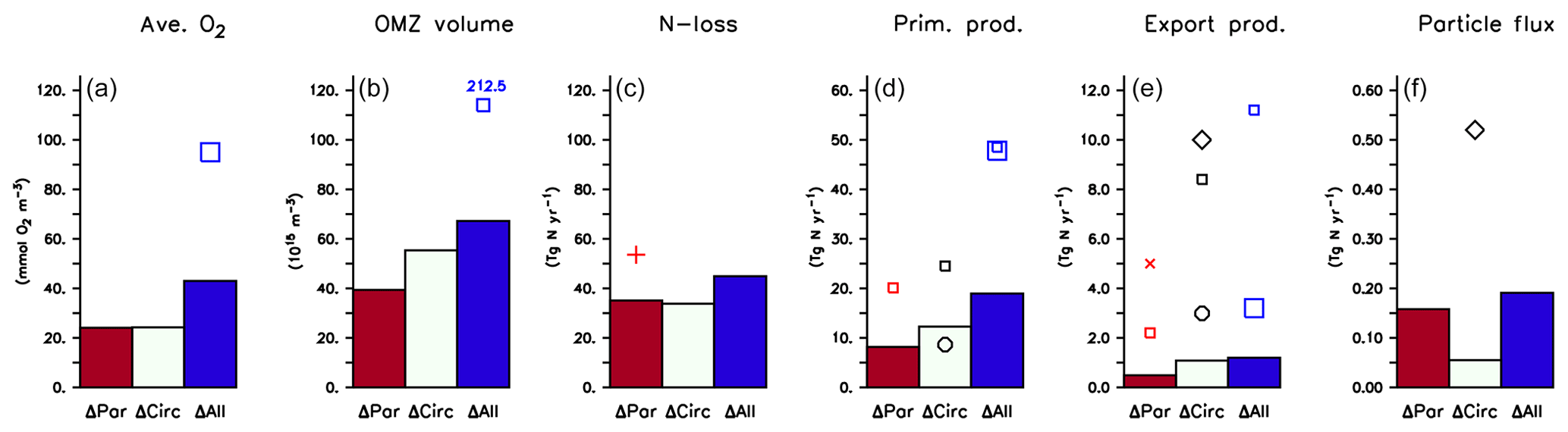
Figure 11 Effect of variation in biogeochemical parameters (ΔPar), circulation (ΔCirc) and across all model experiments (ΔCirc) on (a) global average oxygen, (b) OMZ volume defined by a concentration of <50 mmol m⁻³, (c) global fixed-nitrogen loss, (d) global primary production, (e) export production and (f) organic particle flux at 2000 m, as listed in Table 3. Symbols denote values from Bopp et al. (2013, large squares), Schmittner et al. (2005, small squares), Séférian et al. (2013, circles), Najjar et al. (2007, diamonds), Somes et al. (2013, plus) and Kwon et al. (2009, cross).

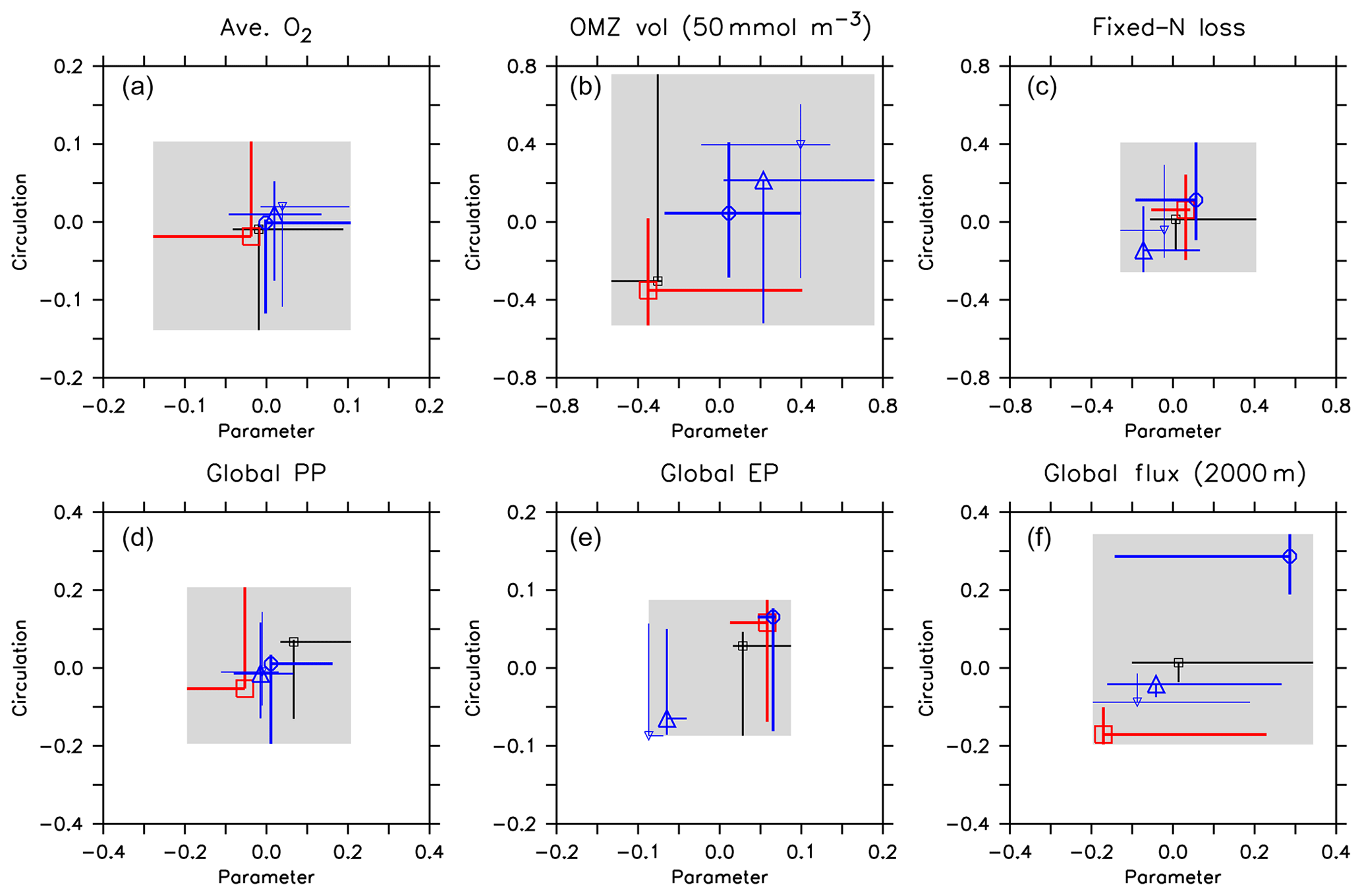
Figure 12 Effect of variation in circulation and biogeochemical parameters on normalised diagnostics. (a) Global average oxygen, (b) OMZ volume defined by a concentration of <50 mmol m⁻³, (c) global fixed-nitrogen loss, (d) global primary production, (e) export production and (f) organic particle flux at 2000 m. All diagnostics X are expressed as relative deviation from mean of the five optimal model simulations ($X_{i,j}/\stackrel{\mathrm{‾}}{X_j^{*}}-\mathrm{1}$), where j and i denote different combinations of circulation j and parameter set i, and $\stackrel{\mathrm{‾}}{X_j^{*}}$ is the average of all optimal model configurations (see Table 3 for values). Each panel shows the range of the normalised diagnostic when the parameter set is kept constant and circulation varied (vertical lines) and when circulation is kept constant and the parameter set is varied (horizontal lines). Symbols denote the optimal model configuration. Colour denotes circulation and optimal parameter set. Black: circulation MIT28 or parameter set of MIT28^*. Thick blue: UHigh and UHigh^*. Medium blue: U20 and U20^*. Thin blue: U17.5 and U17.5^*. Red: ECCO and ECCO^*. Symbols denote optimal model configurations (see also symbol legend in Fig. 6). The grey shaded area shows total variation across all 25 model experiments, corresponding to ΔAll in Table 3. Note that the maximum variation due to the parameter within each circulation (ΔPar of Table 3) is given by the longest horizontal line in each panel. Likewise, the maximum variation due to circulation within each parameter set (ΔCirc of Table 3) is given by the longest vertical line.

Firstly, biogeochemical parameters (ΔPar) as well as circulation (ΔCirc) play an about equally large role for the global average oxygen, which varies by ≈24 mmol m⁻³ (Table 3 and Fig. 11), or about ±15 % of the average optimal value (see also Fig. 12). The variation decreases to less than one-fourth of this value if we restrict our analysis to only optimal models (ΔOpt); as noted above, this strong decrease arises because all optimal models have adjusted $R_{-{\mathrm{O}}_{\mathrm{2}}:\mathrm{P}}$ to account for different ventilation in the high latitudes. Considering all 25 experiments, i.e. accounting for variation induced by both biogeochemical and physical configurations (ΔAll), leads to a variation 6 times as large as for the optimal configurations (ΔOpt).

The variability is much more pronounced when considering the OMZ volume as defined by two criteria, 50 and 80 mmol m⁻³. Again, both circulation and parameter set play an about equally large role; but the impact of changes in parameters or circulation varies across the different models (Fig. 12). For example, applying the parameter set of MIT28^* to a different circulation causes a very strong increase in OMZ volume (vertical black lines in Fig. 12), while model MOPS coupled to the circulation of MIT28 is quite robust with respect to different parameters (horizontal black lines in Fig. 12). On the other hand, when coupled to the ECCO circulation the biogeochemical model is quite sensitive to the biogeochemical parameter set (horizontal red lines in Fig. 12), but its optimal parameter set ECCO^* has a smaller effect when applied to other circulations (vertical red lines in Fig. 12). This diverging effect of parameters and circulation among the different models eventually causes a large spread of 67.2×10¹⁵ m³ of global OMZ volume across all model experiments (ΔAll in Table 3 and Fig. 11), i.e. more than 100 % the observed volume. The effects are even more pronounced when considering a criterion of 80 mmol m⁻³ for OMZ definition (Table 3). The OMZ volume does not show any consistent trend with b, $R_{-{\mathrm{O}}_{\mathrm{2}}:\mathrm{P}}$ or circulation (Fig. 10b), although models with high b and low $R_{-{\mathrm{O}}_{\mathrm{2}}:\mathrm{P}}$ tend to result in a smaller OMZ volume. The circulation of MIT28 shows the lowest OMZ volume.

To summarise, oxygen inventory and OMZ volume are almost equally influenced by physics and biogeochemistry. Optimisation reduces the spread induced by either biogeochemistry or physics to about 30 % for average oxygen, but less for OMZ volume, which varies strongly across all model experiments. We note that the individual contributions of ΔPar and ΔCirc for both diagnostics do not add up to ΔAll (Table 3), indicating that the effects of biogeochemical parameters and circulation are not linear and additive.

3.6 Effect of parameters and circulation on global biogeochemical fluxes

Oxygen and nutrient distributions are influenced by the production of organic matter in the euphotic zone and its subsequent transport to the ocean interior by physical and biogeochemical processes. In addition, denitrification in combination with nitrogen fixation can affect the global nitrogen inventory and the spatial distribution of the nitrate deficit (see Sect. 3.1). Here we finally investigate how these fluxes are affected by the two parameters $R_{-{\mathrm{O}}_{\mathrm{2}}:\mathrm{P}}$ and b.

In our model experiments, simulated global primary production depends slightly more on circulation (ΔCirc) than on biogeochemical parameters (ΔPar; Table 3, Figs. 11 and 12). An increase in b (corresponding to slowly sinking particles) causes primary production to increase (Fig. 10d), likely because of the higher nutrient retention in the euphotic zone, shallow remineralisation and enhanced entrainment of nutrients into the surface layers. Because the last process depends on physical dynamics, we also find an influence of the circulation model on global primary production. Further, our optimisations did not include parameters relevant for plankton dynamics at the surface, which can also explain the comparatively large impact of circulation. The variation across all optimal models of our study (ΔOpt) is much smaller (about one-third) than the variation across all model experiments (ΔAll).

Circulation also plays a large role in export production (particle flux through 100–130 m, depending on model grid), as it supplies new nutrients to the well-lit upper ocean which will, under steady-state conditions, be exported again. Somehow, surprisingly, export production is not strongly determined by b (Fig. 10e). This parameter directly affects the sinking of organic matter out of the euphotic zone. On the other hand, it determines the subsurface concentration of nutrients, as a source for upwelling and entrainment of nutrients. A large b, corresponding to slow sinking and shallow remineralisation, increases nutrients within and below the euphotic zone and thus primary production as the ultimate source of export production; on the other hand, it prevents fast settling of organic particles out of the euphotic zone. Because the plankton parameters were not changed during optimisation, global grazing almost linearly follows primary production (r=0.95), and the statements and conclusions made with respect to the former flux largely apply to grazing (no figure). Therefore, the combined antagonistic effects of b on surface (and subsurface) nutrient turnover, subsurface nutrient concentrations (as a source of nutrient entrainment and mixing) and direct organic particle flux in the upper few hundred metres explain the relatively small variation caused by biogeochemical parameters on export production (ΔPar; Table 3 and Figs. 11 and 12), which is only about half as much the variation due to circulation (ΔCirc).

Deep particle flux, on the other hand, is almost entirely determined by b, and circulation plays a negligible role in this flux (Fig. 10f). The large influence of this parameter is also reflected in its range over all model simulations, which is only slightly larger than the range of flux in optimally configured models (Table 3). Therefore, simulated organic matter supply to the deep ocean and deep nutrient concentrations will, to a large extent, depend on the prescribed particle flux profile, with potential effects on the long-term storage of carbon dioxide.

The loss of fixed nitrogen through pelagic denitrification is tightly related to the extent of OMZs and thus varies quite strongly among the different experiments, with no clear trend for b, $R_{-{\mathrm{O}}_{\mathrm{2}}:\mathrm{P}}$ (Fig. 10c) or μ_NFix (no figure). The range of variation due to parameters and circulation is about equally large (about 50 % of the average optimal global flux; Table 3 and Fig. 11). Overall, this global flux is affected by both circulation and changes in biogeochemical parameters, which induce changes of about ±30 % around the mean optimal flux for each model circulation or parameter set (Fig. 12). Global fixed-nitrogen loss of the optimised models varies much less, likely because optimisation adjusts the parameters to match observed nitrate profiles.

To summarise, at least for this particular biogeochemical model, circulation and biogeochemistry affect global biogeochemical fluxes in different ways. While primary production and fixed-nitrogen loss are almost equally influenced by physics and biogeochemistry, export production depends mainly on physics. Deep particle flux, on the other hand, is affected to a large extent by b. Optimisation reduces the spread induced by changing either biogeochemistry or physics to about 50 % percent for fixed-nitrogen loss and for primary production (compare ΔOpt with ΔCirc or ΔPar). In contrast, there is no such reduction in model variability for export production (which is mainly determined by circulation) or deep particle flux (which is mainly determined by b).

4 Discussion

4.1 Why do different circulations require different parameters?

As we have seen in Sect. 3.2, three optimal parameters depend significantly on three unique diagnostics that result from different features of the circulation model. These diagnostics are related to the northern North Atlantic and the Southern Ocean; the ETP seems to play a lesser role.

The strong correlation of $R_{-{\mathrm{O}}_{\mathrm{2}}:\mathrm{P}}$ with the area of deep mixing clearly confirms that these two model properties (physics and biogeochemistry) regulate global ocean oxygen distribution and inventory in concert. The larger the area of deep mixing, the more oxygen can – or should – be respired in the model, in order to match observed oxygen concentrations. Despite optimisation, the optimal models show an average oxygen concentration of ≈145 mmol m⁻³ in the NPDW (Fig. 9), which is higher than the observed value of 125 mmol m⁻³. Given that the models differ strongly in their physical properties, this residual mismatch of all optimal models, especially in the NPDW, may point towards a deficiency of the biogeochemical model. For example, the spatially homogeneous, and thus inflexible, particle flux profile may not be adequate to simulate the very dynamic response of ecosystem dynamics and particle size structure to regionally variable mixing and nutrient supply (e.g. Guidi et al., 2015; Marsay et al., 2015). Here, a more flexible model resulting in variable sinking speeds of particles (e.g. Gehlen et al., 2006; Niemeyer et al., 2019), or, more generally, spatially flexible remineralisation length scales (e.g. Weber et al., 2016), might be an advantage.

The parameter determining particle flux, b, correlates with the ideal age of NADW (Fig. 6). This physical diagnostic comprises several aspects of circulation: a large area of deep mixing in the northern North Atlantic supplies this region with “young” waters. At the same time, a strong Atlantic Meridional Overturning Circulation (AMOC) and/or confined Deep Western Boundary Current (DWBC) can more quickly export the preformed properties to the southern parts of the basin. Depending on the parameterisation of mixing and other physical processes, biogeochemical tracers are distributed more efficiently in the west–east direction or mixed with deeper waters. When these combined properties of a model cause a long residence time of waters in the NADW, the resulting age of this water mass will be quite high and vice versa.

The circulations applied in our study vary with regard to several aspects in this region: in contrast to all other models the circulation of MIT28 has a large area of deep mixing in the north, including the Labrador Sea (see Fig. 2). There is also a quite strong and wide transport of young waters in the western part of the North Atlantic via the DWBC, as indicated by the southward propagation of relatively young waters between 1500 and 2500 m in the western part of the basin (Fig. 3). At the same time there is a strong lateral spreading of these young waters from the western part (see also Dutay et al., 2002). All processes combined lead to a relatively young average age of NADW in MIT28. ECCO, in contrast, shows only comparatively shallow mixing in the northern North Atlantic (Fig. 2), little southward transport of these waters in the DWBC (Wunsch and Heimbach, 2006) and a large extent of older waters in the eastern tropical Atlantic (Fig. 3). This circulation is characterised by the oldest average age of NADW.

Our optimisations suggest that models with old NADW adjust to a large b or slow particle sinking (for example, b=1.46 of ECCO^*). As ideal age becomes younger, optimal b decreases. Why is this the case? So far, we can not attribute this exclusively to the area of deep mixing (Table 2) or, for example, to the overturning circulation, which is quite low in ECCO (between 13 and 14 Sv; Wunsch and Heimbach, 2006), moderate (17.5 and 18.5 Sv) in U17.5 and UHigh, and high (20 Sv) in U20. Instead, the average age of NADW, and resulting optimal b, likely reflects the combined effects of various model physical and biogeochemical parameterisations: the adjustment of b to smaller values decreases shallow production and remineralisation (see Fig. 10). It also increases export of phosphorus to deep waters and finally to the NPDW (see Fig. 8). Circulation models with high physical turnover in the NADW (e.g. UHigh), as indicated by young NADW, can more easily resupply nutrients to surface waters and therefore balance the loss due to particle sinking in this region.

As shown in Fig. 6, the maximum potential rate of nitrogen fixation μ_NFix increases with area of surface waters defined as $\mathrm{26.5}\le {\mathit{\sigma }}_{\mathit{\theta }}<\mathrm{27.5}$ in the Southern Ocean, i.e. waters reflecting the formation and ventilation of AAIW and SAMW. A broad view of large-scale circulation and the spatial separation of fixed-nitrogen loss and gain helps to understand the adjustment of maximum nitrogen fixation rate to physical processes in the Southern Ocean. Denitrification is a very localised process, occurring mainly in the eastern tropical Pacific (ETP) (Fig. S6). On the other hand, simulated nitrogen fixation takes place throughout large parts of the tropical and subtropical regions of the Pacific, Atlantic and Indian oceans. Even though nitrogen fixation in the Atlantic accounts only for a fraction of global fixed N gain (see also Marconi et al., 2017, for evidence from observations), in our models it nevertheless contributes to the stabilisation of the global fixed-nitrogen budget. A very negative N^*, as arises from denitrification in the ETP, has to arrive in the Atlantic for nitrogen fixation to trigger a competitive advantage of nitrogen fixation. These two regions in the Atlantic and Pacific oceans are connected through large-scale circulation, which transports N^* on centennial to millennial timescales from areas of fixed-nitrogen loss to areas of fixed-nitrogen gain. When passing the CDW of the Southern Ocean, these waters can act as a “mixer of deep waters with distinct isotopic signatures and nutrient stoichiometry” (Tuerena et al., 2015); the resulting mixed properties provide the source of AAIW and SAMW. The subsequent transport via AAIW and SAMW can then trigger nitrogen fixation, e.g. in the Atlantic, and balance the nitrate deficit arising mainly in the Pacific Ocean.

As shown in Fig. 5, the nitrate deficit N^* differs among the different models. For example, MIT28^* exports water with an N deficit of ≈3 mmol m⁻³ from the Southern Ocean to the low latitudes (promoting nitrogen fixation). This model adjusts to a low rate of maximum potential nitrogen fixation of 1.19 $\mathrm{\mu }\mathrm{mol}{\mathrm{m}}^{-\mathrm{3}}{\mathrm{d}}^{-\mathrm{1}}$. On the other hand, UHigh^* simulates SAMW and AAIW that contain a lower N deficit of ≈2 mmol m⁻³, which – depending on phosphate availability – will result in lower nitrogen fixation. The optimal high parameter of UHigh^* of almost 3 $\mathrm{\mu }\mathrm{mol}{\mathrm{m}}^{-\mathrm{3}}{\mathrm{d}}^{-\mathrm{1}}$ can partially compensate for this. The effect of N^* is, however, not consistent across all optimal models: U17.5^* also shows a small nitrate deficit in this region but has a still relatively low maximum nitrogen fixation rate. Here, other effects might play a role, such as a stronger ventilation and consequently younger waters in the ETP (Fig. S2), which induce a smaller OMZ (Table 1), less denitrification in this region (Fig. S6) and thus a lower nitrate deficit in this area, which will eventually be balanced by nitrogen fixation.

In our analysis we have combined the outcrop area of two water masses, SAMW and AAIW, into one single diagnostic. Separating the impact of the two water masses on this parameter, we find that the correlation of μ_NFix with SAMW outcrop area (when defined as $\mathrm{26.5}\le {\mathit{\sigma }}_{\mathit{\theta }}<\mathrm{27.0}$) is less significant (r=0.81) than that with AAIW ($\mathrm{27.0}\le {\mathit{\sigma }}_{\mathit{\theta }}<\mathrm{27.5}$; r=0.88), which is somehow in contrast to the findings by Palter et al. (2010). Their model experiments showed that the largest fraction (between 45 % and 68 %, depending on model configuration) of water volume at the surface between 30^∘ S and 30^∘ N stems from SAMW, highlighting the role of this water mass in nutrient supply in the tropics and subtropics. A possible explanation for this difference between our results and the results by Palter et al. (2010) could be the slightly different definition of water masses. Further, in our models waters denser than σ_θ=26.5 are influenced by the small nitrate deficit of surface waters in the subtropical Southern Hemisphere (Fig. 5), which moderates the signal arising from denitrification in the Pacific.

4.2 Can optimisation help to improve model performance?

As shown in Sect. 3.2, each circulation requires its own set of parameters for an optimal fit to dissolved inorganic tracers. Optimisation facilitates the identification of these constants; on the other hand, it requires many model evaluations, so this approach is prohibitive for models of high resolution because of computational constraints. It would be desirable to optimise a biogeochemical model in a computationally cheaper circulation and then transfer the optimal parameters to a different model that includes more physical details but is computationally more expensive. However, as shown in Sect. 3.3, 3.5 and 3.6, model performance can deteriorate when simulated with non-optimal parameters and result in a considerable spread of the independent diagnostics. Is there any advantage of calibrating biogeochemical models in these rather coarse-scale, simplified circulations, if the parameters are to be transferred to a different circulation? To answer this question, here we discuss the model variability with the background of earlier model studies and observed estimates.

The mean diagnostic across all 25 model experiments (Mean(All) of Table 3) differs only slightly from the mean across only the optimal model configurations (Mean(Opt)) and is close to observed quantities (Table 3), in agreement with Kriest et al. (2017) and Kriest (2017), who found that optimisation against global nutrients and oxygen can help to improve global model performance. Further, the overall maximum variation across all 25 experiments (ΔAll of Table 3) is usually less than 50 % of that found by Bopp et al. (2013), who examined seven global models of different biogeochemical structure and circulation for their global average oxygen, OMZ volume, and primary and export production. This indicates that optimisation can help to improve model performance and reduce its uncertainty, even if parameters were optimised in a different circulation.

4.2.1 Model uncertainty, oxygen inventory and OMZ volume

As shown in Sect. 3.5, changes in circulation and biogeochemical parameters affect model performance with respect to global average oxygen about equally, resulting in an overall variation that is less than 25 % of the observed value (ΔAll of Table 3). In contrast, the global OMZ volume shows a large response to variations in circulation and model parameters and varies by more than 100 % (ΔAll of Table 3) to 200 % (Bopp et al., 2013) of the observed volume. To our knowledge, no global model study exists so far that systematically distinguishes between the effects of circulation and biogeochemistry on global OMZ volume; our study suggests that both are equally important. Even the range across optimal models (ΔOpt) is still quite large, which can be explained by the fact that the target of optimisation (the RMSE to nutrients and oxygen, as of Eq. 1) is only weakly correlated to the fit to OMZs (Sauerland et al., 2019). Application of a revised misfit function, or multi-objective optimisation as presented by Sauerland et al. (2019), can help to better constrain the relevant model parameters and better represent OMZs. Nevertheless, the mean of all models in our study deviates by less than 5 % from the observed mean. Obviously, a good representation of nutrients and oxygen can improve the fit to OMZs to some extent.

However, many global circulation models suffer from a deficient representation of physical processes in the tropics and subtropics, for example in their representation of the equatorial undercurrent (Dietze and Loeptien, 2013), or from inadequate ventilation from the Southern Ocean and North Pacific (see Cabre et al., 2015, and citations therein). The first problem can possibly be cured by a higher resolution, which leads to a more realistic OMZ ventilation by equatorial and off-equatorial undercurrents (Duteil et al., 2014). Parameterisation of intermediate jets (Getzlaff and Dietze, 2013) can also lead to a better agreement of the models. Tuning of biogeochemistry with the background of inadequate physics could compensate for the physical errors but also results in misleading model parameterisations (“overtuning”), with potential consequences for future projections (Löptien and Dietze, 2019). Given the yet unexplored structural and parameter sensitivity of models employed in global assessments, and the large error with respect to OMZ volume and expansion (Table 3; Cocco et al., 2013; Bopp et al., 2013; Cabre et al., 2015), a careful analysis of different error sources (physical and biogeochemical) can help to determine the reasons for model divergence. The study presented here can serve as a first step towards this.

4.2.2 Model uncertainty and global biogeochemical fluxes

The loss of fixed nitrogen through pelagic denitrification is tightly linked to OMZs and therefore also almost equally influenced by circulation and biogeochemical parameters. Our average optimal model estimates are in agreement with recent estimates by Eugster and Gruber (2012) and Somes et al. (2013). The variation due to biogeochemical parameters is lower than found by Somes et al. (2013), who varied the nitrate threshold for denitrification from 20 to 32 mmol m⁻³, i.e. a wider range than identified by our objective parameter calibration (see Table 1).

Average global primary production of the models lies well within the range of observed estimates (Carr et al., 2006) and depends slightly more on circulation than on biogeochemical parameters, similar to the results obtained in the sensitivity study by Schmittner et al. (2005). That study included a wide range of sinking and mixing parameterisations, which might explain the larger variation compared to our results. Applying three different circulations to one biogeochemical model, Séférian et al. (2013) found a spread of primary production which is comparable to our experiments.

Many global model studies analysed the impact of circulation on global export production. Najjar et al. (2007) found an effect of circulation more than 10 times larger than in the present study, which can likely be explained by the nutrient-restoring approach applied in their simple model. Using a more complex biogeochemical model, export production in the study by Séférian et al. (2013) varied only by ≈3 Pg C yr⁻¹, which is closer to the effects of circulation found in our study. The large effects observed by Schmittner et al. (2005) can again likely be ascribed to the wide range of parameterisations tested.

Using a biogeochemical model similar to the one applied by Najjar et al. (2007), Kwon et al. (2009) found an increase in export production of ≈5 Pg C yr⁻¹ when increasing b from 1.1 to 1.4 (about the range tested in our study). Again, this can possibly be explained by the nutrient-restoring approach, which does not account for the interplay between particle export and remineralisation in surface and subsurface layers.

Therefore, our model experiments show a lower sensitivity of global export production on biogeochemical parameters or circulation than the previous studies. Some part of this difference could be explained by the large variation in physical model setup (in the study by Schmittner et al., 2005) or by the very different structure of the biogeochemical model applied (Najjar et al., 2007; Kwon et al., 2009). The large sensitivity of export production in the study by Najjar et al. (2007) also reflects the range of deep particle flux (as diagnosed from export production times 0.052), which is almost 10 times higher than in the present study.

Our experiments suggest that even though circulation does play a large role in export production, deep particle flux is mainly determined by the parameter b. As a consequence, the sensitivity of export production to circulation noted by Najjar et al. (2007) and in the present study does not necessarily imply an equally large sensitivity of deep particle flux (and resulting remineralisation and deep oxygen consumption) on physical model features, which is somehow in contrast to the conclusions drawn by Najjar et al. (2007).

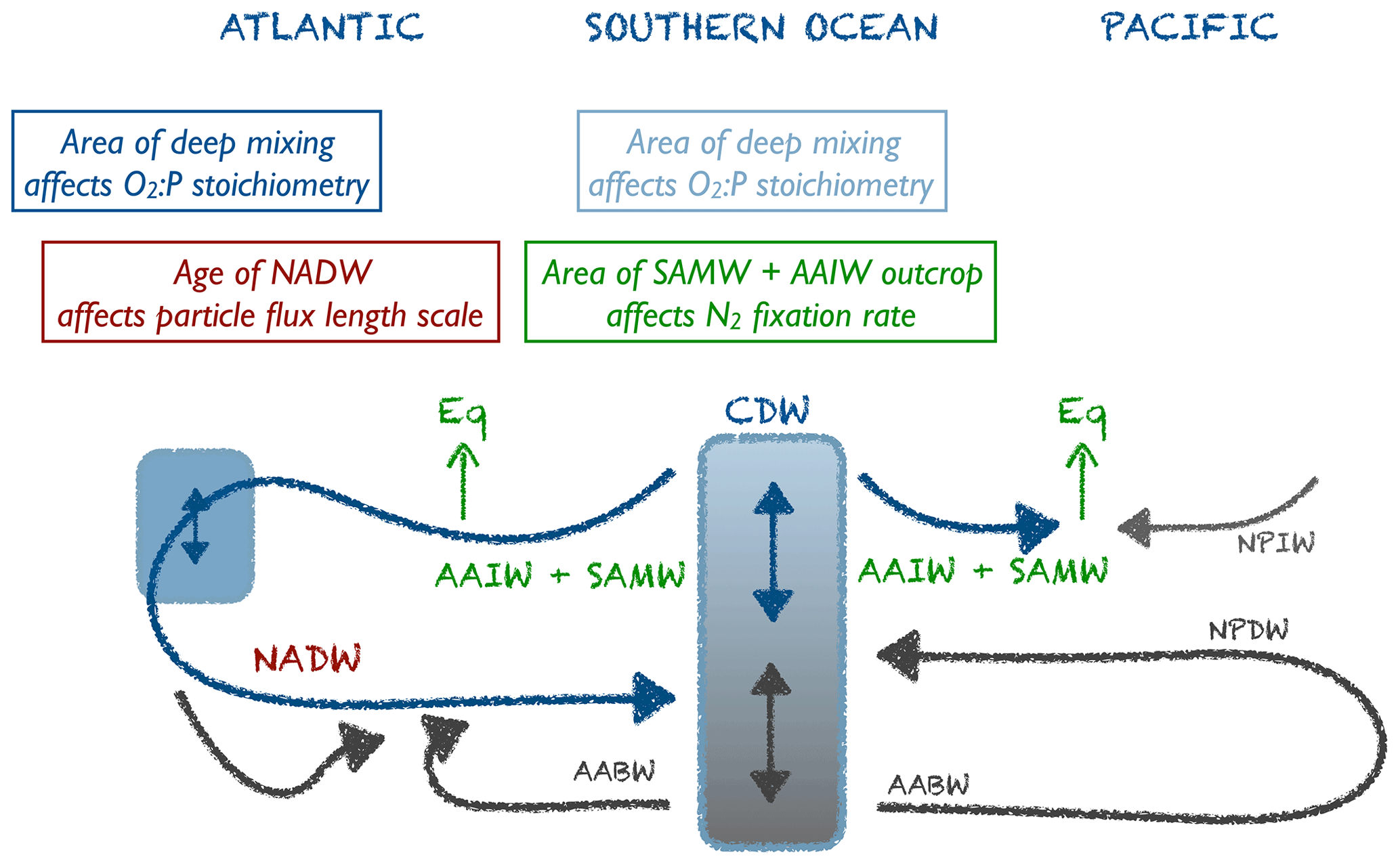
Figure 13 Cartoon depicting the simplified large-scale circulation pattern of the Atlantic and Pacific oceans and the dependence of the three biogeochemical parameters $R_{-{\mathrm{O}}_{\mathrm{2}}:\mathrm{P}}$, b and μ_NFix on physical properties.

4.3 The effect of model complexity

To summarise, in all cases studied here biogeochemical parameter optimisation can help to narrow down the model uncertainty induced by circulation and biogeochemical parameters. Even if parameters optimised in one circulation are later transferred to a different circulation, the resulting spread is mostly around 50 % that of the model intercomparison presented by Bopp et al. (2013). However, that study included models that diverged not only in physics but also in the biogeochemical structure, which might introduce another source of variability. To have a closer look at this we finally contrast the results of MOPS, which we consider to be a model of intermediate complexity, with an equivalent optimisation of a much simpler model “RetroMOPS” presented by Kriest (2017).

RetroMOPS is a four-component model that simulates only phosphate, nitrate, oxygen and dissolved organic phosphorus, but it includes the same structural form for particle flux and remineralisation as MOPS. When coupled to MIT28, and optimised against the same data set and misfit function presented above, the performance and global fluxes of RetroMOPS are very similar to MOPS (in the same circulation; Table 3 and Kriest, 2017). For primary production the difference between RetroMOPS and MOPS is about as large as when MOPS is simulated with different parameter sets within a given circulation. One reason for this is the fact that the optimisation of RetroMOPS by Kriest (2017) aimed only at the parameters related to particle sinking and remineralisation but not at parameters related to phytoplankton growth and loss terms; an additional optimisation of these parameters may likely have produced smaller differences.

Therefore, after optimisation a simple model can perform quite well with respect to large-scale biogeochemical quantities, in agreement with earlier findings (Kriest et al., 2012; Kwiatkowski et al., 2014; Galbraith et al., 2015), illustrating the benefit of parameter optimisation: optimisation allows for a “fair” comparison of models of different complexity (after each model has been tuned to match some desired quantity best); it can therefore also help to decide about the necessary level of model complexity.

5 Conclusions

Optimisation of a global biogeochemical ocean model coupled to five different circulations achieved a good fit to observed nutrients and oxygen with partly different biogeochemical parameters. We identified three parameters that depend significantly on characteristic features of circulation, as summarised in Fig. 13. Areas of deep ventilation in the North Atlantic and in the Southern Ocean determine how much oxygen is supplied to the ocean via air–sea gas exchange and subsequent mixing. As a consequence, optimisation of the model in circulations with vigorous ventilation triggers a high oxygen demand of remineralisation during optimisation. Fast turnover and mixing of NADW, as expressed through low ideal age, affect the parameter responsible for the timescale and vertical extent of remineralisation of sinking particles. Here, models characterised by relatively young waters in the NADW adjust to deeper sinking and remineralisation, with consequences for the large-scale distribution of phosphate. Finally, the combined outcrop area of SAMW and AAIW determines the optimal maximum rate of nitrogen fixation. This may be explained with the role of the Southern Ocean as a “mixer of” waters of different origin and nitrogen deficit (Tuerena et al., 2015). The extent and properties of waters originating from this region (and their fixed-nitrogen deficit), in conjunction with denitrification within the OMZs, then set the stage for the competitive advantage of cyanobacteria in tropical and subtropical waters. Models with a small outcrop area of these waters benefit from a low maximum rate of nitrogen fixation and vice versa. In conclusion, when aiming for a good fit to large-scale biogeochemical quantities, key properties of the underlying circulation model should be considered; depending on region and tracer of interest, these key properties may, however, be different from those of our study.

Cross-validation experiments showed that the optimal parameters could be swapped between the different circulations to a limited extent. Parameters affect biogeochemical model performance in different ways: while the stoichiometric demand of oxygen during remineralisation affects, for example, the ocean oxygen inventory, the particle flux parameter b determines the large-scale distribution of nutrients, in line with earlier studies (Bacastow and Maier-Reimer, 1991; Kwon and Primeau, 2006; Kriest et al., 2012).

Compared to other intercomparisons of global coupled models tuned more subjectively, our overall variation in biogeochemical key properties is at least 50 % smaller, with different contributions from circulation and biogeochemical parameters. For example, export production seems to be mainly determined by circulation, while deep particle flux is determined almost entirely by the particle flux parameter b. Other biogeochemical diagnostics are affected more or less equally by circulation and biogeochemical parameters. Finally, OMZ volume is very sensitive to changes in circulation and biogeochemical parameters and varies most strongly across all model experiments.

However, models considered in global intercomparisons usually also differ in their biogeochemical structure and complexity. Our experiments suggest that after optimisation the differences due to model structure are much smaller than those due to model parameters or circulation. This indicates that a simpler model can perform as well as a more complex model (with respect to the metrics and diagnostics applied here), similar to the results obtained by Kriest et al. (2012), Kwiatkowski et al. (2014) and Galbraith et al. (2015). It also illustrates how biogeochemical parameter optimisation can aid model development: whenever new components or parameterisations are introduced to a global model, this new model has to be tuned in order to match observations on global or regional scales. Often, the choice of appropriate parameters is not easy and requires extensive testing and sensitivity analysis. Automatic (algorithmic) optimisation can make calibration more efficient, simplifying the search for a good model match to observed quantities. For a given misfit function it can also support decisions about the necessary level of model complexity.

Therefore, our experiments suggest that global biogeochemical ocean models benefit from optimisation, even if this was carried out in a circulation differing from that of the “target” circulation. However, to date there is no guarantee that a model showing a good fit to observed quantities in steady state (i.e. when simulated in a pre-industrial or present-day climatological physical forcing) will exhibit the correct response when applied to transient scenarios reflecting future climate change. As shown here and in earlier studies (Cocco et al., 2013; Cabre et al., 2015; Löptien and Dietze, 2019), OMZs seem to be particularly sensitive to both biogeochemical and physical parameters. Accounting for the match between simulated and observed OMZs during optimisation can reduce the model spread in steady state (Sauerland et al., 2019). Extending the simulation of optimal models to future states could then inform us about their sensitivity to changes in circulation and forcing and may provide a better constraint on their uncertainties. Thus, the study presented here serves as a first step to unravel the uncertainties associated with the divergence of global biogeochemical model performance and uncertainty.