Megafauna community assessment of polymetallic-nodule fields with cameras: platform and methodology comparison

With the mining of polymetallic nodules from the deep-sea seafloor once more evoking commercial interest, decisions must be taken on how to most efficiently regulate and monitor physical and community disturbance in these remote ecosystems. Image-based approaches allow non-destructive assessment of the abundance of larger fauna to be derived from survey data, with repeat surveys of areas possible to allow time series data collection. At the time of writing, key underwater imaging platforms commonly used to map seafloor fauna abundances are autonomous underwater vehicles (AUVs), remotely operated vehicles (ROVs) and towed camera “ocean floor observation systems” (OFOSs). These systems are highly customisable, with cameras, illumination sources and deployment protocols changing rapidly, even during a survey cruise. In this study, eight image datasets were collected from a discrete area of polymetallic-nodule-rich seafloor by an AUV and several OFOSs deployed at various altitudes above the seafloor. A fauna identification catalogue was used by five annotators to estimate the abundances of 20 fauna categories from the different datasets. Results show that, for many categories of megafauna, differences in image resolution greatly influenced the estimations of fauna abundance determined by the annotators. This is an important finding for the development of future monitoring legislation for these areas. When and if commercial exploitation of these marine resources commences, robust and verifiable standards which incorporate developing technological advances in camera-based monitoring surveys should be key to developing appropriate management regulations for these regions.

1 Introduction

The increasing demand for tech metals for consumer and industrial high-technology devices has again stoked interest in the potential use of global deep-sea polymetallic-nodule fields as exploitable sources of these materials in the near future (Yamazaki and Brockett, 2017; Peukert et al., 2018a; Volkmann and Lehnen, 2018). This increasing interest, simultaneously driving the technological development of marine mining equipment and the granting of exploration contracts within the Clarion–Clipperton Fracture Zone (CCFZ) (Lodge et al., 2014), has stimulated several recent European research projects (e.g. JPI Oceans MiningImpact 1–2 and MIDAS). These projects focused on the study of these remote ecosystems to better understand the nodule distribution (Peukert et al., 2018b) as well as the community structure of macrofauna (De Smet et al., 2017) and megafauna (Simon-Lledó et al., 2019b), ecosystem functioning, and susceptibility to damage following anthropogenic perturbation and/or resource removal (Vanreusel et al., 2016; Jones et al., 2017). Despite the occurrence of nodule fields in the Atlantic, Pacific and Indian oceans, the majority of research efforts have been focused on the CCFZ, located in the northern–central Pacific, as it has the highest known density of nodules (Mullineaux, 1987; Jones et al., 2017; Simon-Lledó et al., 2019b), and the Peru Basin (southern–central Pacific) (Bluhm, 2001; Purser et al., 2016; Simon-Lledó et al., 2019a). Both regions have been considered to potentially host commercial abundances of nodules at some point in history. Focused scientific study commenced in the 1980s, with simulated mining studies conducted in both areas, to assess the response of fauna to mining activities (Lam et al., 2006). These studies are summarised in Jones et al. (2017), with the “DISturbance and COLonization” (DISCOL) long-term study in the Peru Basin being the most extensively perturbated region of seafloor studied to date (Thiel, 2001). Prior to the 1980s, only occasional opportunistic fauna collection records had been published from these areas. Since the 1980s, regular biological box core sampling has been conducted in the CCFZ, whereas the majority of fauna sampling in the DISCOL area has been image based, augmenting some initial trawl sampling deployments. The DISCOL experiment was designed to simulate the effects that physical disturbances, such as those caused by future commercial deep-sea mining, might have on the seafloor and its inhabitants. In 1989, a plough harrow was used to create a large-scale disturbance on the seafloor in the DISCOL experimental area (DEA). The plough harrow was deployed 78 times in 1989, with the aim of driving all polymetallic nodules from the sediment surface into the underlying soft sediments (Fig. 1) (Bluhm, 2001). This ploughing action destroyed the majority of surface megafauna and drove manganese nodules within 8 m diameter swathes down into the sediments. As a result, fauna that lived attached to the nodules was removed and thus destroyed. The soft-bottom community, however, did show signs of recovery 7 years after the plough disturbance. Several monitoring cruises of the impacted areas commenced in the following years and decades. The repopulation of the disturbed areas by highly motile and scavenging animals started shortly after the area was ploughed (Bluhm, 2001). Seven years later hemi-sessile animals had returned to the disturbed areas, but the total abundance of soft-bottom taxa was still low compared to the pre-impact study. However, nearby reference areas not impacted by the experiment indicated pronounced temporal variability in megafauna communities in the region (Bluhm, 2001). The ploughing activities also created a sediment plume that resettled in the surrounding areas. In these indirectly impacted areas, animal densities declined immediately after the ploughing event, and although densities later (i.e. after 3 and more years) appeared to be greater than in the pre-impact study reference areas (Bluhm, 2001), megafaunal community composition in these areas remains significantly different than that found within plough tracks and reference areas (Simon-Lledó et al., 2019a). As has been reported from many ecosystems, the methodologies used to quantify fauna abundances and species diversity can greatly influence assessments. This challenges the direct comparison of regions sampled differently (Lam et al., 2006; Wilson et al., 2007; Murphy and Jenkins, 2010; Jaffe, 2014). Further, small variations in deployment techniques or sampling set-ups (e.g. variables such as mesh size or trawl speed for direct sampling, illumination, camera and lenses for remote sampling) can also influence the quality of the collected data (Purser, 2015), hampering comparison within the same study site. In this study, a range of commonly used imaging platforms were deployed at varying altitudes above the seafloor to survey megafauna across a defined region of the DEA, which is a region of the Peru Basin with abundant seafloor nodule coverage. These collected images were then placed into the online image annotation system BIIGLE (Langenkämper et al., 2017), and the fauna was identified in the different image sets by five annotators using a predetermined taxon catalogue. The hypothesis tested was that both composition and abundance observations of fauna differ between different imaging methodologies in polymetallic-nodule fields. This study aims to provide useful information and guidance on how future optical monitoring of these and other remote ecosystems should most effectively and efficiently be conducted, should commercial exploitation of these remote resource fields commence.

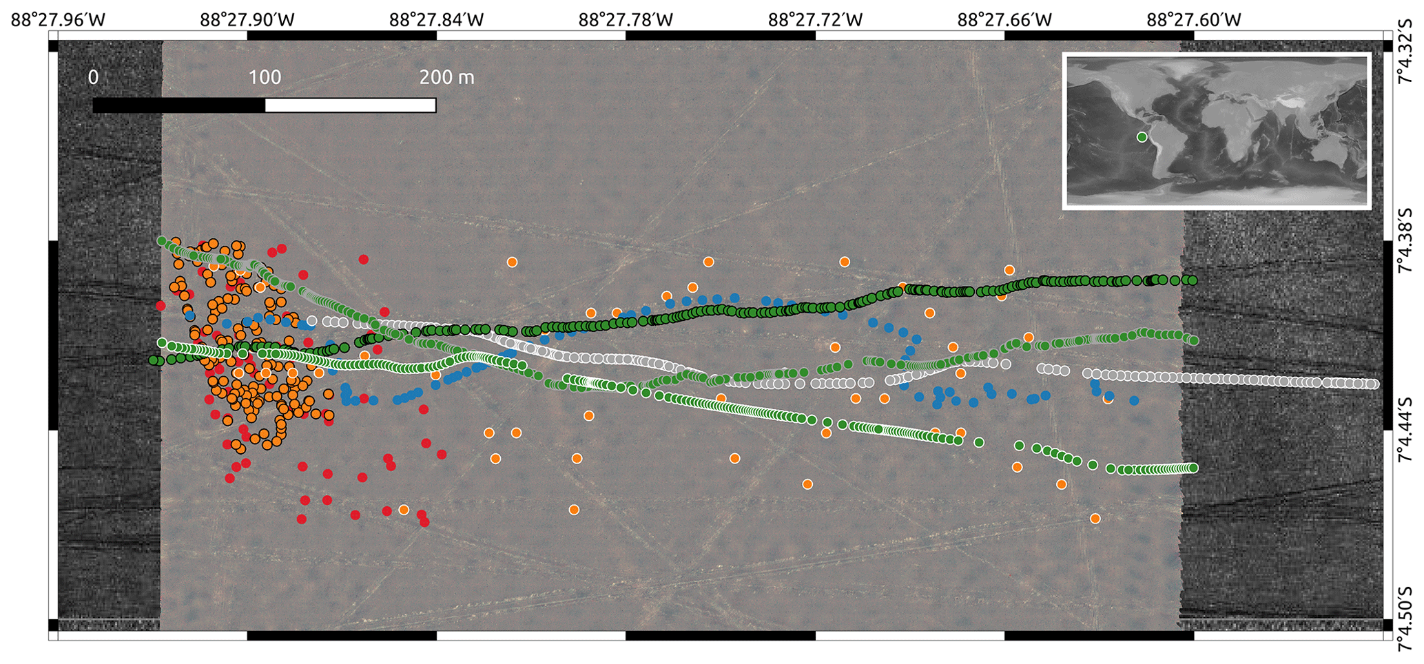
Figure 1 Overview map of imaging locations of the eight different datasets. DS_A (green dots, grey border), DS_B (green dots, black border), DS_C (blue dots), DS_D (green dots, white border), DS_E (orange dots, black border), DS_F (grey dots), DS_G (orange dots, white border) and DS_H (red dots). The world map in the top right corner shows the geographical location of the DISCOL area in the eastern South Pacific (green dot; © NOAA, Amante and Eakins, 2009). The study area covers ca. 600 m×150 m. The background map shows another photo mosaic, created from the full image set of which DS_G is a subset. Criss-crossing lines are plough tracks by the mining simulation in 1989.

1.1 Polymetallic nodules and associated fauna

Polymetallic nodules, as well as representing a potential commercial resource (Burns and Burns, 1977; Watling, 2015; Petersen et al., 2017), are a key hard substratum that, in combination with the background soft sediment, act to increase habitat complexity and promote the occurrence of some of the most biologically diverse seafloor assemblages in the abyss (Vanreusel et al., 2016; Simon-Lledó et al., 2019c). Nodule fields at the abyssal Pacific can be comprised of nodules of up to 25 cm in diameter (Sharma, 2017) and at a range of abundance densities (e.g. 0–30 kg m⁻²; Mewes et al., 2014). Processes of nodule formation are uncertain, though each individual nodule tends to form around a small shell fragment, shark tooth or equivalent small hard foci. With growth, individual nodules become heavier and capable of supporting, as an anchor or hard substrate, a range of larger filter-feeding organisms (Tilot et al., 2018; Simon-Lledó et al., 2019c), such as sponges (stalked – Kersken et al., 2018; encrusting – Lim et al., 2017), stalked and non-stalked crinoids, soft and hard corals (Cairns, 2016), xenophyophores (Gooday et al., 2017), sabellid worms, etc. (Bluhm, 2001). Sessile organisms in turn support a diverse array of mobile and sessile epibenthic organisms, including further sponges, corals and worms as well as mobile and semi-mobile fauna such as amphipods, isopods, anemones, brooding octopodes (Beaulieu, 2001; Purser et al., 2016) and many others (Vanreusel et al., 2016). Although soft-sediment stalked sponge fauna is found in nodule-abundant regions, the nodule-based epifauna supports increased local biodiversity and abundance of species. In addition to providing a hard substrate for living attachment, nodules also increase the range of hydrodynamic niches available to the local ecosystem fauna (Mullineaux, 1989) and add complexity to food fall transport pathways. Recent cruise observations from the DISCOL region showed rapid transport of dead pyrosomes, following a surface bloom, to the seafloor (Boetius, 2015). These dead pyrosomes were then hydro-dynamically trapped by benthic currents alongside nodules, providing a local food supply to the nodule community which might otherwise have been transported from the region by the ambient benthic flow conditions. This flow dynamic variability also impacts the habitat niches available for infauna (across all infauna size classes) below and surrounding the nodules, with their presence influencing local biogeochemical activity and oxygen penetration pathways. At this crucial time point in research into polymetallic nodules and associated fauna, it is important to highlight also the gaps in current knowledge and that any management plans developed should take these shortfalls into consideration. At the time of writing it is clear even from the sparsity of published megafauna papers from nodule regions that these ecosystems are not all alike. The Peru Basin region of the South Pacific seems to support a generally higher abundance of stalked fauna than the Clarion–Clipperton Fracture Zone (CCFZ) nodule domains (Bluhm, 2001; Vanreusel et al., 2016). Some large types of megafauna, such as benthic octopodes, have thus far only been observed within these nodule ecosystems in the South Pacific (Purser et al., 2016), as have some fish species (Drazen et al., 2019), despite the recent increased sampling effort across the CCFZ. Conversely, the abundant sessile sponges recently characterised from the CCFZ, Plenaster craigi, (Lim et al., 2017), are not apparent in images or analysed samples collected from south of the Equator. Whether these discrepancies are due to oceanographic, nutrient or habitat niche differences is not yet known. It may be considered that the larger nodule sizes found in the Peru Basin region are more suitable as anchors of sufficient stability for stalked fauna to allow brooding by octopodes for the hypothesised years required by deep-sea incirrates (Purser et al., 2016). Another major absence in the scientific dataset is sampled voucher specimens from nodule provinces. Opportunistic direct sampling by remotely operated vehicles (ROVs) has taken place on a limited scale, though the ground-truthing of image and video data collected by ROVs and autonomous underwater vehicles (AUVs) at the species level is, at present, not possible. Though this is an obvious disadvantage over direct sampling of the seafloor (e.g. by trawl) to determine the present fauna mix, this is perhaps to some extent countered by the far larger areas which may be surveyed rapidly by towed and remote camera systems – an important point given the extremely sparse distribution of many fauna individuals of morphospecies in nodule ecosystems (Bluhm, 2001; Vanreusel et al., 2016; Purser et al., 2016; Simon-Lledó et al., 2019b). These sparse distributions make impact assessments more problematic than for denser fauna categories, which have historically been subject to the direct impact by the offshore fishery or petrochemical industries, such as coral and sponge reefs, where atolls and accumulations can be directly surveyed pre- and post-cruise, either via imaging or direct sampling (Purser, 2015; Howell et al., 2016; Huvenne et al., 2016). Whether future management plans favour a direct or an image-based monitoring approach to megafauna diversity and stock assessment, the requirement to fill these holes in extant voucher specimen collections from these regions is equally prescient.

1.2 Potential impacts associated with nodule extraction

Nodule collection will locally remove the major source of hard substrates in nodule field areas, rendering the remaining habitat unsuitable for some fauna (i.e. suspension feeders), as observed in experimental mining studies in the CCFZ (Vanreusel et al., 2016; Jones et al., 2017) and DISCOL areas (Simon-Lledó et al., 2019a). Further, depending on the removal technique, the seafloor will likely be perturbed, with compaction tracks potentially formed and all overcast by plume deposits (Jones et al., 2017; Sharma, 2019). These features will increase the complexity of biogeochemical activity in the region (Paul et al., 2018) and influence local hydrodynamic conditions. Experimental tracks made with both an epibenthic sled (Greinert, 2015) and plough harrow (Bluhm, 2001) have created seafloor micro-topography which focused the deposition of salps following a surface bloom event which occurred during SO242-2 (Boetius, 2015). Such localised food input variability in the deep sea will likely result in a further modification of the fauna communities found in these exploited regions.

1.3 Methodologies for fauna abundance assessment

Box coring and multicoring are common survey methods in impact assessments and monitoring programmes, conducted to assess impacts on small fauna (e.g. less than 1 cm) following an anthropogenic impact event (Gage and Bett, 2005). For larger fauna, image-based surveys usually provide much more accurate estimations of benthic taxa richness and numerical density than traditional trawling techniques (Morris et al., 2014; Ayma et al., 2016) and have no direct physical impact on the ecosystem being investigated. When planning to assess polymetallic-nodule fauna abundance following commercial exploitation of these remote resource fields, the associated human impacts of monitoring programmes should be as little as possible. We therefore focus within this paper on the contrasting suitability of various image-based approaches for assessing fauna abundance in polymetallic-nodule ecosystems. Furthermore, image data can be made publicly available to regulators, interested NGOs and other players easily via online platforms (Langenkämper et al., 2017), allowing these stakeholders to conduct their own studies or analyses with the same primary data. To assure reliable monitoring, contractors need to publish data including uncorrupted location and timing metadata. The acquisition technology of that metadata needs to be fraud-proof (e.g. by incorporating navigation data into the imagery). In case of monitoring activities utilising directly collected fauna from box core, multicore or ROV collection, much of the material will be processed once, by one lab, and can degrade during the processing steps, preventing further studies. Image data also facilitate the straightforward archiving of collected data (Schoening et al., 2018) for later comparison with subsequent images, potentially collected up to decades after experimental or industrial disturbance, to assess long-term recovery rates. Given the extremely long lifespans of many deep-sea organisms (Roark et al., 2009; Norse et al., 2012), this is an important consideration when developing monitoring strategies for efficient and useful impact assessment within these ecosystems.

1.4 Factors determining the quality of deep-sea image data

Samples collected by box cores, multicores or trawl are directly related to the surface area sampled. In this case, the type of trawl or corer may influence the comparability of the results to some extent (i.e. net size and tow speed important for trawls, closing mechanism for box corers). For image-base derived data, there are possibly a greater number of factors affecting the estimations of fauna abundance. The most significant of those are introduced below.

1.4.1 Camera optics

The area of seafloor which may be imaged by an optical platform is determined by the lens parameters used in the camera system, distance and orientation to the seafloor, sensitivity of the system to motion and illumination, and a range of other factors (Jaffe, 2014). Larger areas of the seafloor can be imaged with wide-angle or “fisheye” camera systems (Kwasnitschka et al., 2016), though there is an associated vignetting effect rendering the details collected from the extremities of an image less rich than areas of seafloor more directly located below the lens centre (Purser et al., 2009; Cauwerts et al., 2012). The raw images collected by those camera systems can appear quite distorted, and manual labelling of fauna within these images is more difficult towards the edges of each image. Digital post-processing of these distorted images can be reasonably straightforward when the arrangement of optics for an imaging platform is known, and for larger fauna these processed images can be suitable for subsequent analysis (Schoening et al., 2016a, 2017). However, image processing cannot create “newly improved” data, and therefore there will always be a loss of information at the image extremities after lens correction. Image analysis could therefore focus on central parts of the image, and the boundary area of images could be used to display, for example, navigation metadata. Lenses of a more “telephoto” or narrower angle will allow collection of less distorted images, though these collected images will capture a significantly smaller area of seafloor than may be achieved with wider-angle systems.

1.4.2 Illumination and power provision

The deep sea is a dark environment with no sunlight penetration. It is therefore essential that camera systems are supplemented by artificial illumination. To provide sufficient illumination for video and still-camera systems, abundant power reserves must either be mounted on the platform or delivered via a cable from the support vessel. The amount of power which can be provided to a platform is determined by a range of design and operational parameters. AUVs for example must remain reasonably lightweight and must carry sufficient power to provide mobility and to take images at depth. Towed camera systems, in contrast, are always attached to a cable (e.g. coaxial, fibre-optic) which may provide sufficient power for continuous seafloor illumination. Positioning of the lights on an imaging platform can be difficult, and optimising the spread of light, i.e. maintaining an equal light balance across the imaged area, can be challenging. Illumination vignetting can be partially addressed prior to analysis by excluding the image edges from analysis (Purser et al., 2009; Marcon and Purser, 2017). Given that AUVs must carry all required power (for mobility and imaging) with them, this can result in a less-than-optimal illumination of the seafloor (see Sect. 1.4.3). There is no doubt that light-emitting diode (LED) technology will become more efficient, but at present these prevalent lower-light-condition datasets constrain the seafloor resolution which may be achieved during imaging surveys. Additionally, when the lights and camera are mounted close to each other, a significant amount of light might be scattered by the water column into the camera, leading to a degraded “foggy” image, which is an issue for small platforms and/or high-altitude photography. Finally, the colour spectrum of the light also needs to be considered, as for instance the returned yellow, orange and red components of the signal may be too weak to support taxonomic identification, depending on the type of light source. The illumination system needs to be set up to accommodate the target altitude of the camera platform above the seafloor as well as the expected altitude variation.

1.4.3 Platform altitude

The distance to an object can greatly alter the quality of an image. Although this may sound like a straightforward parameter, it may play a hugely important role when analysing fauna abundances in an area. Maintaining a uniform altitude throughout and between survey deployments is highly desirable (i.e. to standardise the object and/or fauna detectability rates) but may be difficult. In regions of the World Ocean where the seafloor is highly complex, such as at deepwater coral reefs (Purser et al., 2009) or within canyon systems (Orejas et al., 2009), it can be a struggle to maintain an equal distance from camera optics from towed, autonomous, remote and submersible-based imaging platforms to the seafloor. For polymetallic-nodule fields, however, the seafloor is generally fairly uniform in depth, with very gentle slopes more the norm than occasional sudden slopes or cliff walls. Even so, towed platform altitude stability can be greatly influenced by operator skill, experience, environmental conditions (i.e. wave conditions at surface) or ship infrastructure (winch operational parameters and presence or absence of heave compensators). AUV imaging platforms are improving in stability and mission planning at a rapid rate (McPhail et al., 2010; Yu et al., 2018), and maintaining flight altitudes is now a standard surveying procedure. Operations with these expensive devices tend to err on the side of caution; ground tracking is often set with a conservative 5–10 m flight altitude. At these higher flight altitudes, more light is required to illuminate the seafloor than when a comparable AUV is deployed close to the seafloor (see Sect. 2.1.6).

1.4.4 Data volume

Pioneer image-based studies in polymetallic-nodule fields were conducted with analogue film-based camera systems (although live, black and white seafloor views were provided to towed systems via a basic TV camera set-up) (Bluhm, 2001). This limitation constrained deployments to the collection of a few 100 s of images. At present, camera systems can deliver many images per second, even under low-light conditions. This potentially high flow of image data, however, requires either an adequate digital storage space on the imaging platform (Kwasnitschka et al., 2016) or the facility to be transferred directly to a shipboard storage system (Purser et al., 2018). This increased data flux allows for more complete spatial studies of the seafloor to be made with an imaging platform, but to get this additional information from the dataset, increased processing time is required.

1.4.5 Dataset resolution

Image resolution is derived from a combination of the camera optics and the deployment altitude and allows comparing image datasets numerically. The camera optics determine the pixel resolution (usually in the tens of megapixels for state-of-the-art camera systems). The field of view of the camera objective lens and the deployment altitude determine the image footprint, i.e. the area in square metres that is covered by a single image acquisition. These two values can be combined to a measure of megapixels per square metre (MP m⁻²) or the numerically identical pixels per square millimetre to analyse the annotator performance and fauna density estimates consistently.

1.4.6 Time series studies

To determine the level of impact an event has had on a specific region of seafloor, repeated visits to a locale are required. It is important to conduct baseline and impact monitoring surveys in a region-specific manner to accommodate differences in faunal composition. Baseline information acquired in one nodule area (e.g. the CCFZ) cannot directly be transferred to another (e.g. the Peru Basin). Ideally, a number of surveys at differing times of the year would be conducted before an impacting event to gauge the background fauna community of a region and to identify natural variation and seasonality in community patterns. These baseline studies would be followed by repeated surveys at different time points during and after the impacting event. These repeated visits should allow quantification of the duration and recovery of impacts. Planning such a study may sound straightforward, but given the remoteness of many deep-sea regions, getting the same equipment and survey crew together may be difficult. One such study, aimed at gauging the impact of oil and gas exploration drilling on cold-water coral reefs on the Norwegian margin, visually surveyed a number of reefs on five occasions (Purser, 2015). Despite these five survey cruises taking place within a 3-year period in a relatively accessible area of the Norwegian shelf, each cruise used different ROV systems and survey protocols. Analysis of collected data was further complicated by the mounting of different camera and illumination systems on each ROV and contrasting flight altitudes and dive plans being used for each deployment.

2 Methodology

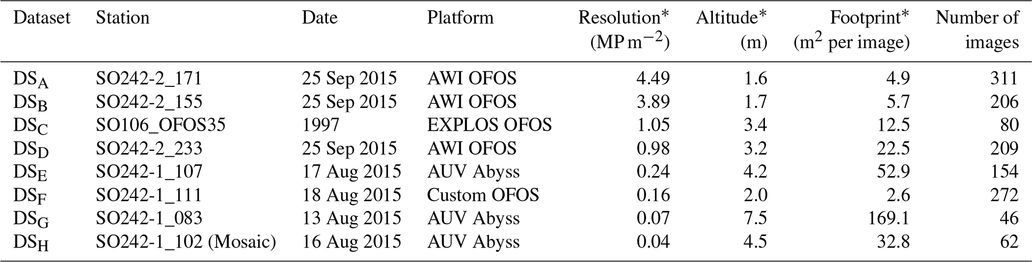
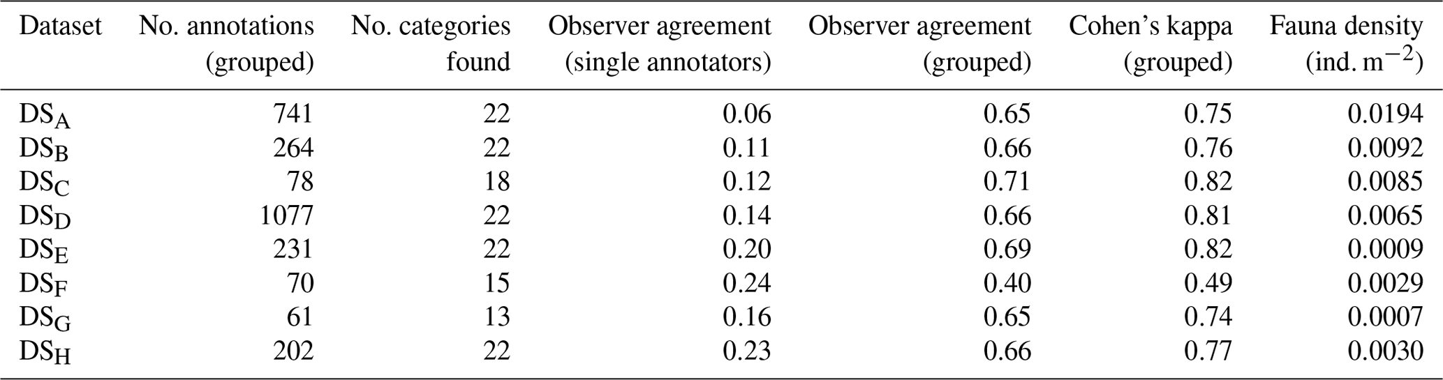
For this comparative study of the effectiveness of various imaging platforms for assessing megafauna abundances in polymetallic-nodule ecosystems, eight distinct image datasets, DS_A to DS_H (see Table 1), were collected. All datasets were acquired in a discrete area of seafloor of ca. 600 m×150 m. These eight datasets were collected by three different towed camera platforms (one of which was deployed at several altitudes above seafloor) and an AUV (deployed at two different altitudes above seafloor) during three research cruises. One dataset (DS_C) was acquired during RV Sonne cruise SO106, and the other seven were acquired during RV Sonne cruises SO242-1 (DS_A, DS_B, DS_D) and SO242-2 (DS_E–DS_H) in 2015. DS_H was created by producing a mosaic of the seafloor from overlapping AUV imagery and then dividing the mosaic into smaller image tiles for fauna analysis. All image sets were analysed by five annotators, a₁–a₅, using a predesigned fauna catalogue to label a selected group of 20 fauna categories ω_a–ω_t within each discrete image (see Fig. 2). The term category refers to an arbitrary object type, extending across various taxonomic levels and also including the category litter. The group of annotators selected the 20 categories by including fauna that is frequent enough for statistical interpretation. The 20 categories neither cover all objects visible in the images nor represent all the fauna known to occur in the area. The majority of categories represented morphotypes and could thus potentially include different cryptic species. Numbers of annotations per category and per dataset vary. No organism size cut-off was defined for annotation; instead the image resolution determines which size of objects are still discernible. From this labelling effort, the densities of the various identified fauna categories in each dataset were statistically compared.

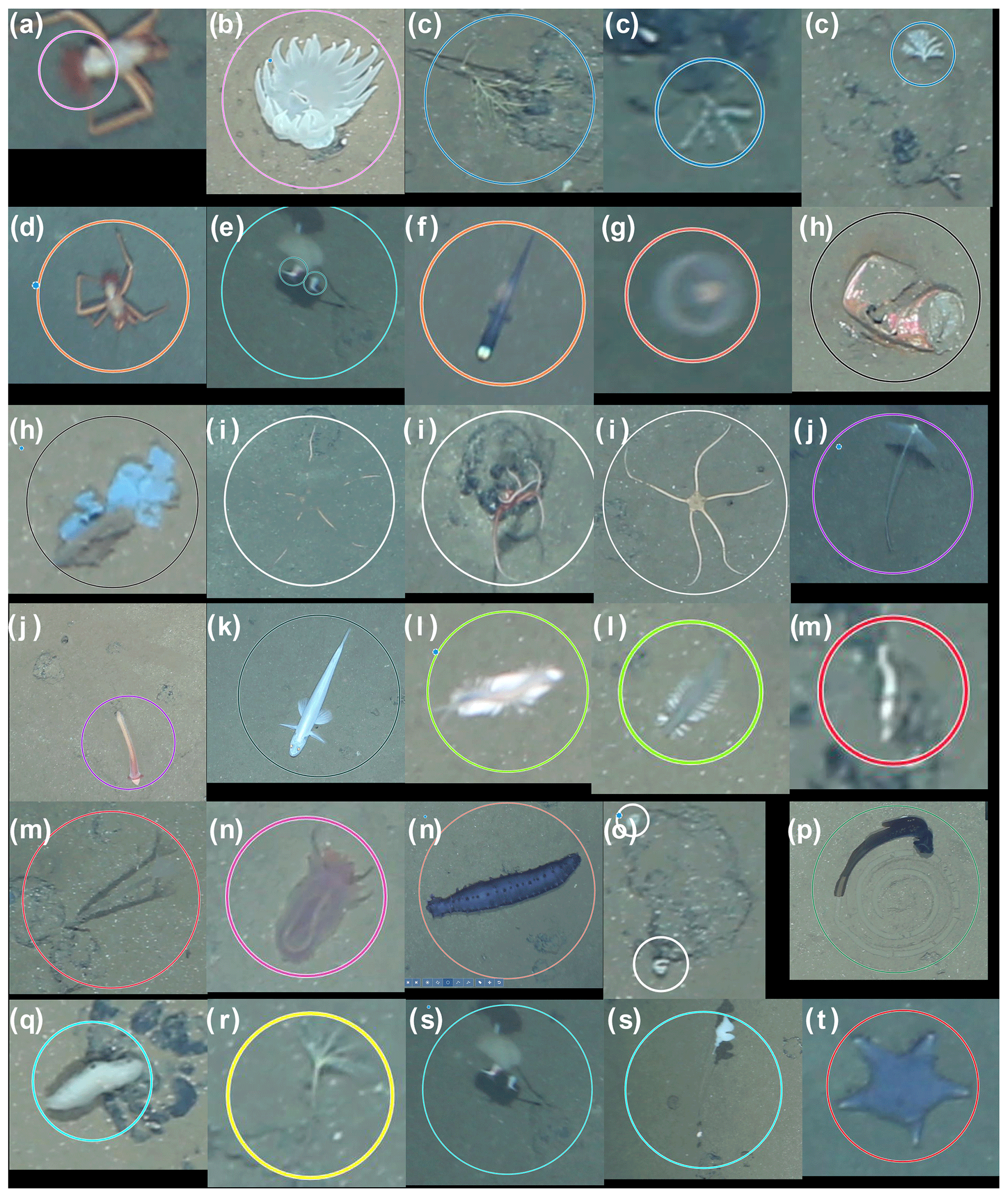
Figure 2 Fauna categories used in the current study for the DISCOL area. Circles correspond to annotations in BIIGLE. Colours of annotations visualise the category type. (a, b) Anemones, (c) corals, (d) crustacea, (e) epifauna, (f) Ipnops fish, (g) jellyfish, (h) litter, (i) Ophiuroidea, (j) Cladorhizidae, (l, p) Enteropneusta, (k) fish, (l) Polychaeta worms, (m) Polychaeta tubeworms, (n) Holothuroidea, (o) small encrusting, (q) Porifera, (r) stalked crinoid, (s) stalked Porifera and (t) Asteroidea. All examples were scaled for visualisation purposes; some, like (l) and (m), are small and close to the resolution limit.

Table 1 Summary of image data collected for each dataset considered in this study. Columns marked by (^*) represent median values across the dataset.

2.1 Imaging platforms, resolutions and deployment altitudes

2.1.1 DS_A (4.49 MP m⁻²) and DS_B (3.89 MP m⁻²): low-altitude imagery from AWI OFOS camera sled

Towed still-image and video sleds are equipment often used for gleaning some information on seafloor physical and megafauna community structure (examples can be found in Fig. 3a, b, d). These platforms consist of a solid frame which is connected to a survey vessel by an umbilical cable, in most cases capable of supplying power and data transfer between the ship and the platform. To operate, an altitude above the seafloor is set by the users as a function of seafloor topographical structure, items of interest, vessel speed and weather conditions. A winch operator maintains the appropriate flight altitude above seafloor as the survey vessel tows the device over the requested course. These systems can utilise reasonably simple cable systems to allow live TV signals from the seafloor to reach a towing support vessel or modern fibre-optic cables through which high data loads can be transmitted in real time. The simplicity and relatively low costs of these towed systems, coupled with their moderate personnel requirements, have made them an attractive choice to use in scientific expeditions, particularly in time series studies, where the same equipment is required for each revisit to a location. For this current study, the Alfred Wegener Institute – Helmholtz Centre for Polar and Marine Research (AWI) – Ocean Floor Observation System (OFOS) was used for collection of several datasets (see Table 1). Developed for time series analysis of the HAUSGARTEN marine time series station, the system has seen 15 years of regular use, and numerous megafauna fauna papers have been published based on collected data (Bergmann et al., 2011; Pham et al., 2014; Purser et al., 2016; Taylor et al., 2016, 2017). The AWI OFOS consists of a solid frame containing vertically downward-facing still-image and video cameras (Fig. 3). Additionally, the system mounts LED lights to a supply light for the video camera as well as powerful flash units to allow 26 MP still images to be taken from an optimal altitude of 1.5 m above the seafloor. The AWI OFOS also incorporates three parallel lasers to allow seafloor coverage (and fauna sizes) to be quantified in the images and video data collected. Figure 4a and b show typical images collected from the DISCOL area from an operational altitude of 1.6 m (DS_A) and 1.7 m (DS_B).

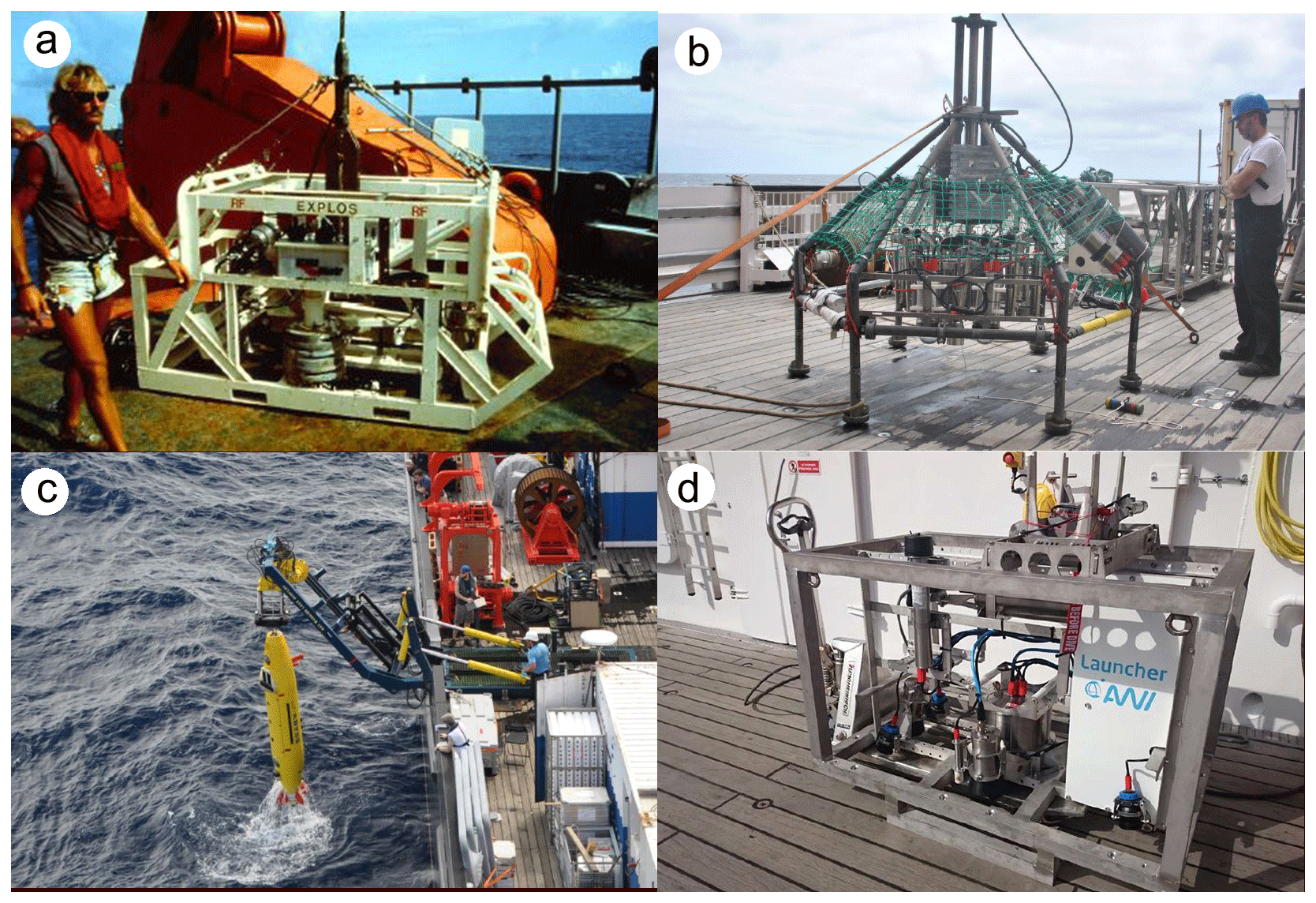
Figure 3 Imaging platforms used in the current study. (a) The EXPLOS OFOS analogue camera sled from 1997 (Schriever and Thiel, 1992). (b) A custom OFOS used during SO241-1. (c) GEOMAR AUV Abyss. (d) AWI OFOS.

Figure 4 Example images of datasets DS_A–DS_D, with platform information and mean image footprints as follows. (a) DS_A – OFOS – 4.9 m². (b) DS_B – OFOS – 5.7 m². (c) DS_C – OFOS – 12.5 m². (d) DS_D – OFOS – 22.5 m².

2.1.2 DS_C (1.05 MP m⁻²): high-altitude, digitised analogue imagery from EXPLOS camera sled

Prior to the equipping of research vessels with fibre-optic cables, allowing HD video to be transmitted directly to the support vessel during a dive, it was common practice to set up a low-quality video link to the seafloor to allow the operators of a towed device to maintain an appropriate flight altitude above the seafloor during a deployment. The scientific data collected were still images manually triggered from the ship but recorded onto analogue photographic film using a PHOTOSEA 5000 camera mounted on the “Exploration System” (EXPLOS) towed device. This required the mounting of actual film canisters on the towed platforms, resulting in deployments with fewer than 400 images collected (the capacity of standard, extended 35 mm magazines of the era). In 1989, after the seafloor ploughing, such an analogue towed camera rig was used to image in the DISCOL area (Fig. 3a). The 1989 dataset was recently digitised by the MiningImpact project of the Joint Programming Initiative Ocean (JPIO) and made available for this study. An example image is given in Fig. 4c.

2.1.3 DS_D (0.98 MP m⁻²): high-altitude imagery from AWI OFOS camera sled

With increasing distance from the seafloor, a particular optical system can image a greater area for a given set of optics, assuming that correct focusing, for example, can be achieved. With a doubling of distance, however, effectiveness of illumination is reduced by 75 %. For towed systems this may be compensated for by additional supply of power or a greater number of lights. For the current study, however, the same AWI OFOS introduced in Sect. 2.1.1 was redeployed with the same standard lighting configuration at a flight altitude of 3.3 m. Figure 4d shows a typical seafloor image taken from this altitude.

2.1.4 DS_E (0.24 MP m⁻²): low-altitude imagery from AUV Abyss

During SO242-1, GEOMAR's AUV Abyss (Linke and Lackschewitz, 2016) was deployed for several photographic mapping missions (see Fig. 3c). The vehicle's original camera had been replaced by a Canon 6D DSLR camera and the Xenon strobe by an LED flash system (Kwasnitschka et al., 2016), placed 2 m from one another. The low-altitude vertical imagery of DS_E was captured from a target altitude of 4.5 m, at a speed of 1.5 m s⁻¹ and at a frame rate of 1 Hz. The system was equipped with a Canon 8–15 mm fisheye lens (fixed to 15 mm) centred in a dome port. Owing to weak illumination in the outer image regions, only the central 90^∘ (across track) or 74^∘ (along track) of the fisheye images were used and trilinearly resampled to a picture that an ideal rectilinear 18 mm lens would have taken. An example picture is shown in Fig. 5a.

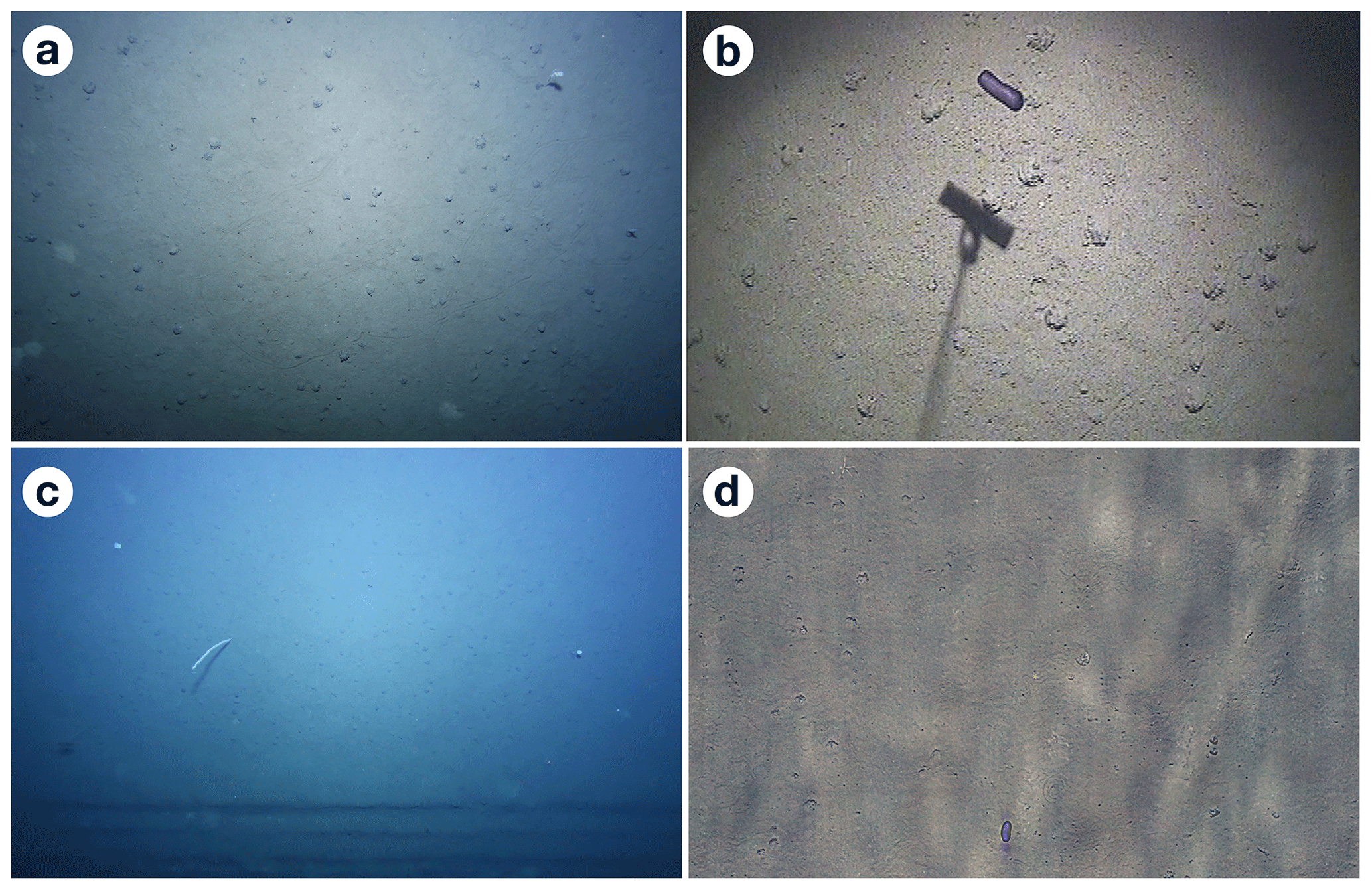
Figure 5 Example images of datasets DS_E–DS_H, with platform information and mean image footprints as follows. (a) DS_E – AUV – 52.9 m². (b) DS_F – OFOS – 2.6 m². (c) DS_G – AUV – 169.1 m². (d) DS_H – AUV – 32.8 m².

2.1.5 DS_F (0.16 MP m⁻²): low-altitude imagery from custom OFOS camera sled

During SO242-1 the area of interest was surveyed with a colour video camera (Oktopus GmbH) in conjunction with one Oktopus HID 50 light mounted vertically on a towed frame (see Fig. 3b). The signal was transmitted to a deck unit (Oktopus GmbH VDT 3) and recorded using an external video converter (Hauppauge – HD PVR), which converted the signal to .mp4 files, and was then recorded on a PC using ArcSoft TotalMedia Extreme software. For this study, frames were extracted from these video files at a rate of 0.1 Hz. The custom OFOS was put together in an “ad hoc” fashion, from a range of off-the-shelf components, to mimic “pioneer” image-based methodology rather than a fully designed and integrated device. An example image is given in Fig. 5b. Further details of the custom OFOS and its deployments can be found in Greinert (2015).

2.1.6 DS_G (0.07 MP m⁻²): high-altitude imagery from AUV Abyss

As a result of the fixed distance of roughly 2 m between the camera and light source on AUV Abyss, images taken by the above system at higher altitudes increasingly suffered from very strong backscatter in addition to the loss of colour resulting from the large distance from the light source to the seafloor and back into the camera. Although the AUV imaged at altitudes above 10 m, those images were deemed of a quality unsuited for fauna analysis. Consequently, besides the 4.2 m “low-altitude” AUV imagery in DS_G, AUV imagery acquired at 7.5 m altitude represents the dataset of maximum altitude in this contribution. Apart from the different altitude, all capture parameters in DS_G remained the same as in DS_E. An example image for this dataset is shown in Fig. 5c.

2.1.7 DS_H (0.04 MP m⁻²): low-altitude imagery from AUV Abyss and extracted from a photo mosaic

AUV images of station SO242-1_102 were collected at ca. 4.5 m above the seabed, with 80 % along-track and 50 % across-track overlap in order to build one large photo mosaic out of the images. In order to mitigate water and illumination effects otherwise dominant in the final mosaic, a robust statistical estimate of the illumination component was performed. For this, each image was robustly averaged with the seven images taken before and after, producing an image without nodules that represents the illumination effects. The raw image was then – pixel-wise – divided by the illumination image and multiplied by the expected seafloor colour, which was obtained from box core photographs of the same cruise. For each track of a multi-track AUV mission, the images were registered against each other, leading to relative AUV localisation information with sub-centimetre accuracy. Afterwards, the photos were projected to the seafloor and rendered into a virtual orthophoto with a resolution of 5 mm per pixel (reflecting the best resolution in the fisheye images) of roughly 7 ha size. The photo mosaic was then subdivided into ca. 11 000 tiles and uploaded to BIIGLE for megafaunal assessment. An example tile is shown in Fig. 5d. A similar mosaic of the same area was used in Simon-Lledó et al. (2019a).

2.2 Image annotation methodology

Within the study, 1340 seafloor images (or mosaic tiles) were analysed for megafauna abundance and community structure estimation (see Table 1). All images used in the study were imported into the BIIGLE online annotation system (Langenkämper et al., 2017). Once imported, five annotators inspected the images independently and annotated objects by placing a circle around each instance using the BIIGLE annotation interface (see Fig. 6). To assist in this, an identification guide with 20 categories was produced (see Fig. 2), from which the annotators could work.

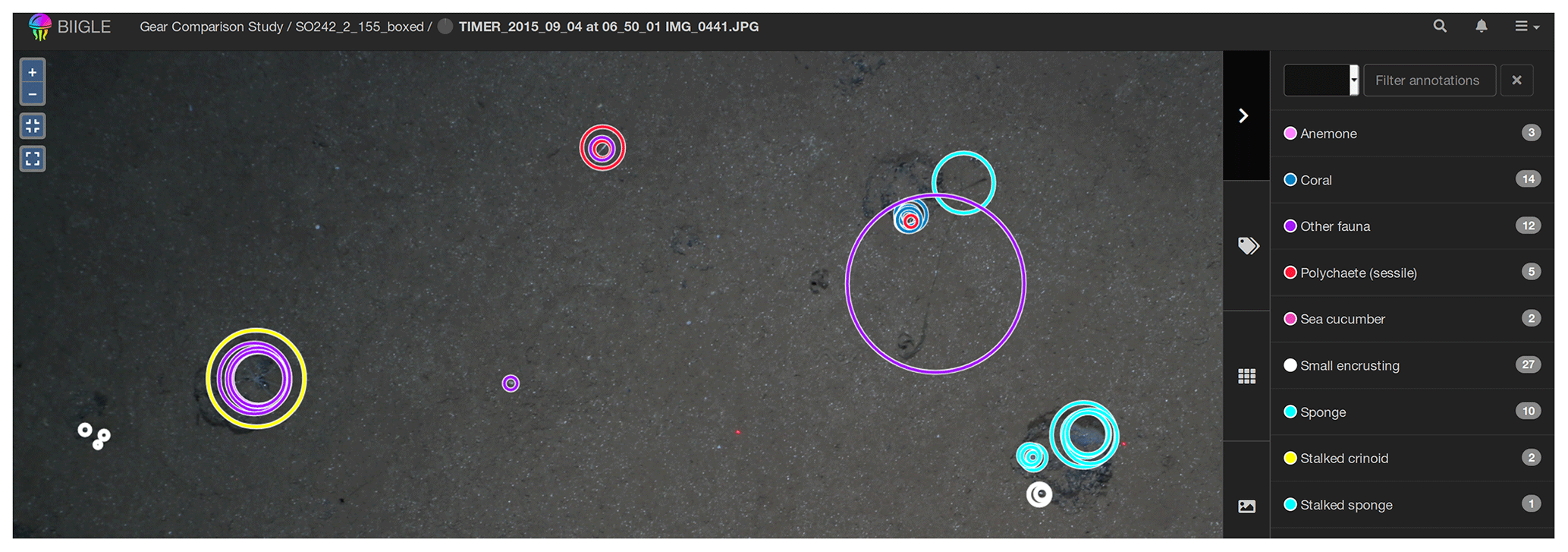
Figure 6 Circular fauna identifications made by several operators using the BIIGLE software application. Each circle corresponds to one annotation by one annotator. Colours of circles correspond to categories.

2.3 Observer agreement

Manual annotation was conducted independently. To compare results from the five annotators, a₁ to a₅, inter-observer agreement was computed (Schoening et al., 2012). First, the individual annotations of each pair of annotators were compared regarding the annotation location (i.e. the detection step) and annotation label (i.e. the classification step). Annotations of individual experts were then grouped to gold-standard annotations to increase the robustness of the dataset comparison. A gold standard is the best-possible ground truth information if no actual ground truth is available (Schoening et al., 2016b). Grouping of annotations was conducted by fusing annotations which overlap within one image and are of a similar size to one grouped annotation. The position and radius of a grouped annotation represent the mean of the positions and radii of the single, overlapping annotations. The support of one annotation quantifies how many experts found this individual and thus ranks between 1 and 5. The label of the grouped annotation was selected as the most frequent label within the grouped annotations. Annotations that were supported by only one annotator were discarded. Also, if no two annotators assigned the same label to an annotation it was discarded. As a further measure of observer agreement, Cohen's kappa was computed (McHugh, 2012).

2.4 Fauna-specific statistical analysis

The average abundance estimations of each individual fauna category computed for each of the eight image sets were derived from the annotations made by each independent annotator. The five density estimates obtained for each fauna category, as generated from the labels made by the individual image annotators across the eight imaging-platform datasets, were compared using nonparametric Kruskal–Wallis tests. These tests were conducted using the software package SPSS 17.0. Significant differences were considered when p<0.05.

3 Results

3.1 Aggregated results for datasets

Aggregated results for various characteristics of the eight datasets and annotations were computed by averaging across all fauna categories (see Fig. 7 and Table 2). All figures except Fig. 7g further visualise the results of the grouped annotations. Most obvious is the increase in fauna density with imaging resolution (see Fig. 7a). This trend is mirrored in the observation that the median size of the annotated fauna decreases with increasing resolution (see Fig. 7b). Together it can be reasoned that the increased resolution allows annotating smaller objects, increasing the total amount of individuals annotated. Nevertheless, it is also obvious that the increased resolution comes with an increase in observer disagreement. Figure 7c shows that the standard deviation of fauna densities created by the five experts increases with increasing resolution. Figure 7d–f highlights the trade-off between resolution and seafloor inspection effort. In Fig. 7d it can be seen that the increase in resolution comes with a decrease in acquisition efficiency in terms of the area per hour (m² h⁻¹) that can be imaged. This negative correlation exists also when removing dataset DS_G. Figure 7f shows that, although higher densities of fauna are detected for high-resolution datasets, it still requires manually inspecting more megapixels per annotation compared to lower-resolution datasets. The annotation effort for such high-resolution datasets is thus overproportionately large. Removing single points that appear as outliers in the different data dimensions (Fig. 7a–l) does not change the general trends of the correlation lines.

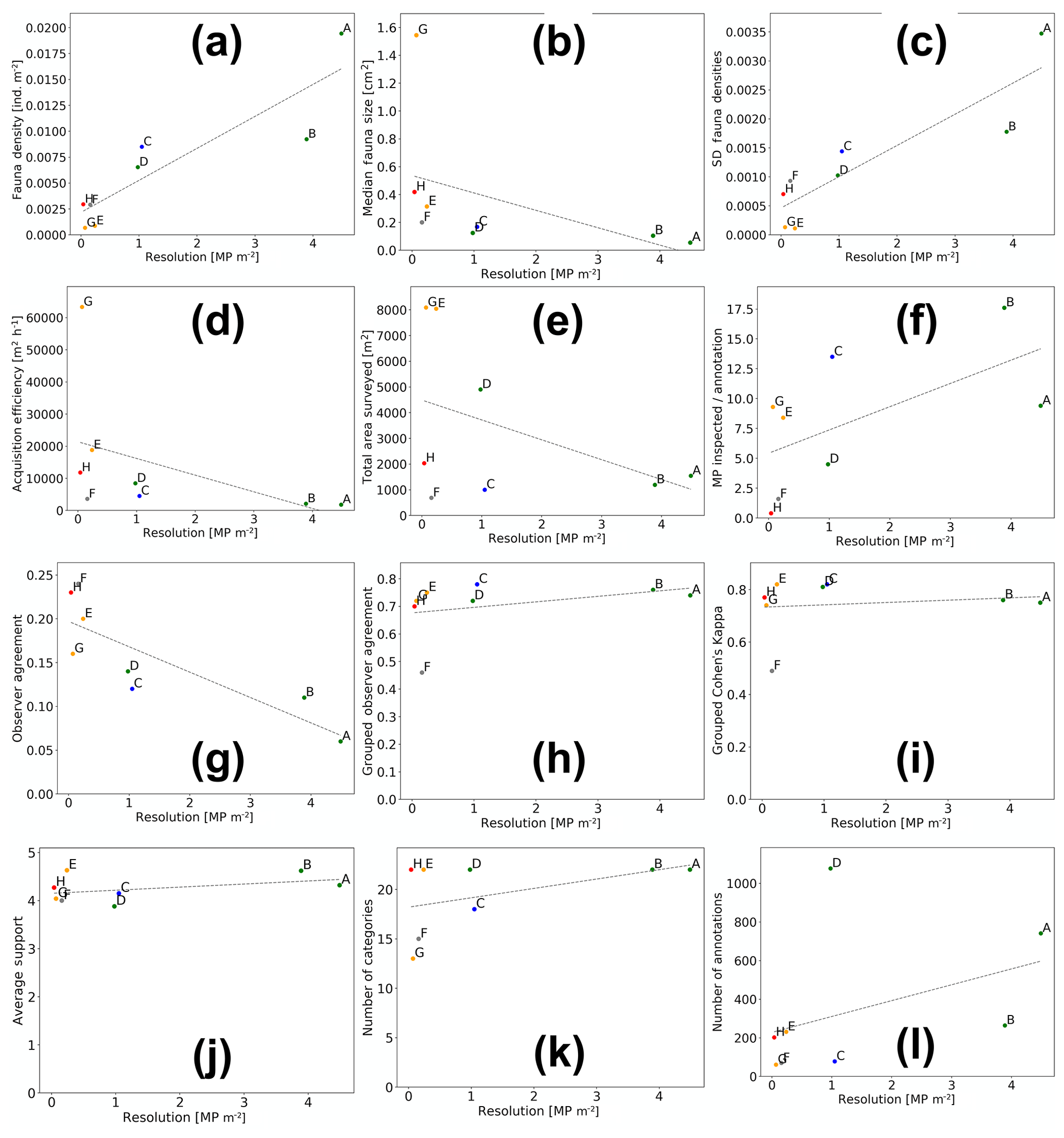
Figure 7 Aggregated results of fauna annotations for the eight datasets (dots A–H; green: AWI OFOS; blue: EXPLOS OFOS; grey: custom OFOS; orange: AUV Abyss; red: AUV Abyss mosaic). Dashed lines show linear regressions.

Table 2 Annotation results for the eight different datasets considered in this study.

3.2 Observer agreement

Figure 7g outlines the importance in image-based studies of incorporating annotations created by more than one annotator. It shows the generally poor observer agreement in this study when considering the single-expert annotations (see also Table 2). It further highlights that the observer agreement drops with increasing image resolution, echoing the results in Fig. 7c. When grouping the single observer annotation to form the gold-standard annotations, the observer agreement increases significantly (see Fig. 7h). This increase is similarly reflected by Cohen's kappa values: all but one above 0.7, which is deemed to be “substantial agreement” (0.6–0.8).

3.3 Fauna-specific statistical analysis

The seafloor densities of the 20 categories of fauna and seafloor features, as quantified by the five independent annotators, are given in Fig. 8 (mobile fauna) and Fig. 9 (sessile fauna). Kruskal–Wallis tests indicated that for all fauna categories (with the exception of “molluscs”) observed, individual densities differed by imaging platform at the 95 % threshold (“small encrusting”, “starfish”) or <99 % threshold (all other fauna categories). For sessile fauna, the average individual densities observed were highest across fauna categories in DS_A. Generally, the average densities for this dataset acquired at 1.6 m altitude were roughly double to triple those observed in DS_B, which was collected in the same year from a slightly higher median altitude of 1.7 m. Densities of sessile fauna derived from AUV data were generally lower than those derived from OFOS data. Sessile-fauna densities derived from AUV data acquired at 4.2 m altitude (DS_E) were invariably higher than those derived from 7.5 m AUV data (DS_G). Sessile-fauna densities determined from the mosaicked images were roughly equivalent or a little lower than the densities determined from both uncombined AUV datasets (see Fig. 9). For mobile fauna, trends in densities of fauna categories were less dependent on the observing platform. Even though differences were indicated as significant for many fauna categories (see Table 3), these differences were not clearly relatable to either imaging-platform deployment altitude or methodology and observers (see Fig. 8).

Table 3 Kruskal–Wallis test assessment of whether differences in fauna abundance derived from the DISCOL seafloor data are significant for each fauna category used in the current study. H is the test statistic, N is the number of observers, df is degrees of freedom (i.e. number of data types compared −1) and p is significance. P values of less than 0.05 indicate significance at the 95 % percentile.

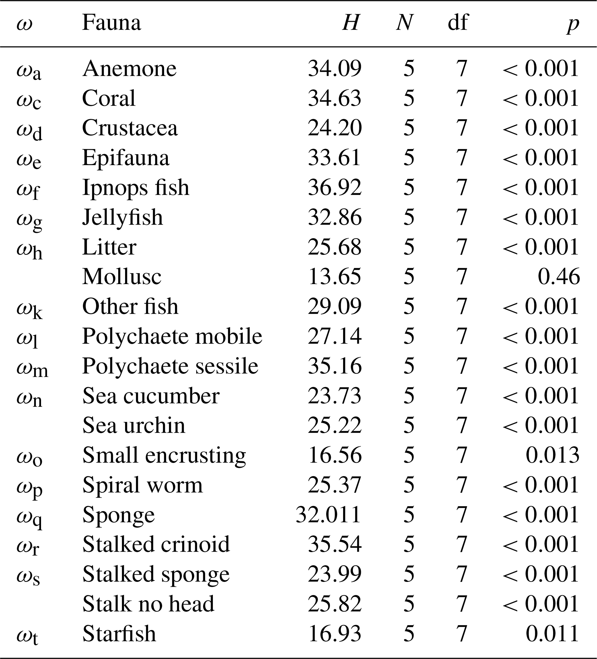
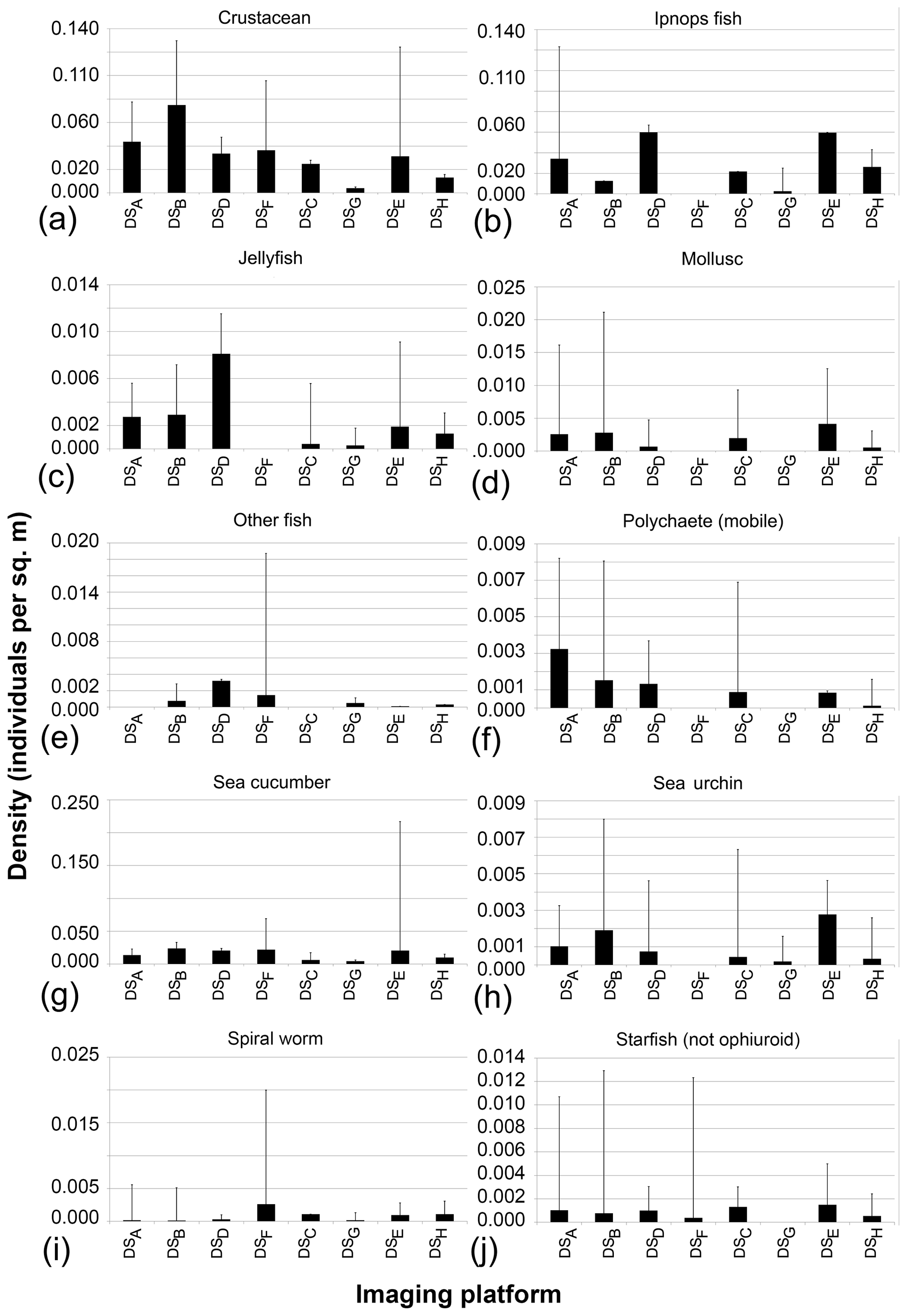
Figure 8 Mobile-fauna abundances averaged across five annotators that independently annotate image data collected during the eight survey deployments.

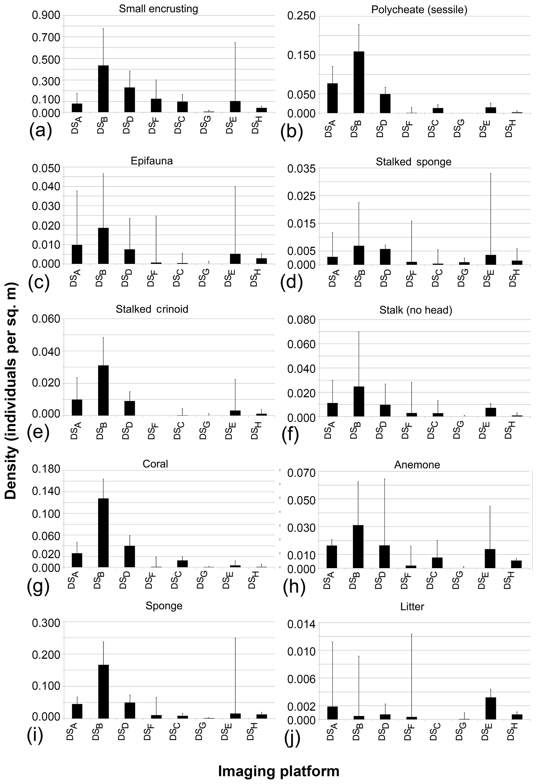
Figure 9 Sessile-fauna abundances averaged across five annotators that independently annotate image data collected during the eight survey deployments.

4 Discussion

4.1 Spatial and temporal factors

The current study attempts to estimate the effectivity of a range of imaging devices across an overlapping area of seafloor based on experts' manual annotations. Given the inaccuracies of about 1 % achievable with the POSIDONIA underwater positioning system used for the majority of imaging deployments (Peyronnet et al., 1998) and the lack of distinct seafloor features in the DISCOL polymetallic-nodule province, sampling exactly the same areas of seafloor was not possible. Nevertheless, due to the reasonably homogenous nature of the seafloor (from the scale of metres to hundreds of metres) in the survey region, it seems likely that comparable organisms were present across areas. Temporal differences in community structure, particularly between years, cannot be wholly discounted as explanatory factors of differences between datasets (Bluhm, 2001; Borowski, 2001). Highly mobile fauna, such as fish and jellyfish, can vary in local abundances on temporal scales of minutes, and even the less mobile ophiuroids and holothurians can respond relatively swiftly to changes in seafloor conditions, such as a food fall or hydrodynamic conditions. Even so, we assume that temporal and spatial differences between the collected data are of minor significance in explaining the differences in densities observed.

4.2 Deployment altitude and image resolution

Even though it was not possible to deploy all platforms at different altitudes within the same cruise, it was feasible to collect material altogether from both the AUV (two altitudes) and the AWI OFOS (three altitudes). For virtually all fauna categories used, the highest-density estimates were made from data collected at the lowest deployment altitude and highest pixel resolution. At these altitudes, less water is present between the camera and the target, reducing distortion and light attenuation effects. The only exceptions to this trend were the highly mobile, water-column-dwelling fauna, such as jellyfish and fish. Given the three dimensionality of the habitat utilised by these organisms, observation from a greater altitude is beneficial, and it is thus more likely to image such fauna. This is potentially coupled with avoidance mechanisms triggered by the lights on the imaging platform or the sound of thrusters (in the case of the AUV deployments). The way in which fauna density estimations are subject to the deployment altitude does not appear to be linear or comparable across fauna categories. Larger types of fauna, such as “stalked sponges” (see Fig. 9d) and “starfish” (see Fig. 8j), were spotted with equivalent ease across all datasets, whereas smaller types of fauna, such as “sessile polychaetes” and “sponges” (see Fig. 9b and i), were annotated more frequently in data collected from lower altitudes. These altitude-based trends in density estimation were observed in both AUV and OFOS datasets. Interestingly, an average deployment altitude difference of just 10 cm, from 1.7 to 1.6 m average altitude between SO242-2 OFOS deployments, corresponded to a much greater difference in fauna density estimations than the 1.6 m difference in deployment altitudes between the 3.3 and 1.7 m datasets. Both the attenuation of light in water and the variable impact of this reduction on the wavelengths of reflected light, as well as the size of the fauna image received by the camera, likely play a role in determining the fauna abundance accuracy achievable from a dataset. This extreme subjectivity to deployment altitude of derived density estimations is an important consideration when comparing results from different deployments.

4.3 Annotator skill and observer effect

To label fauna at a species level from imagery requires a certain amount of skill and awareness of the fauna likely to occur in a particular survey region. In many cases, annotation categories will only refer to morphotypes. This is due to the fact that most fauna in the areas is either still unknown or impossible to identify from images alone. Properly assessing fauna occurring in a habitat, especially when addressing human impacts, requires not only ecological expertise but also support from taxonomists. Nevertheless, even when specialists analyse the same dataset, inter-observer differences in annotations can be significant (Schoening et al., 2012; Durden et al., 2016). Here, however, differences between platform altitude proved to be more significant than the observer effect for all faunal categories. Therefore, given the sparsity of many deep-sea taxa in nodule provinces (Simon-Lledó et al., 2019b), the use of key species is of more applicability when determining monitoring strategies for impact assessment, where statistically significant differences in abundances may reflect differences in populations of pre-impacted or control areas and those within impacted areas. These key types of fauna are likely to differ between different locations and ecosystems. For deep-sea manganese nodule provinces, the level of understanding of ecosystem functioning is probably insufficient for selecting species and/or taxa of major importance for the ecosystem. Certainly, some easily annotated types of fauna play important roles as habitat engineer species, such as the stalked fauna, which add the vertical axis to increase habitat niche availability (Purser et al., 2016; Vanreusel et al., 2016). Biogeochemical processes within and at the sediment–seawater interface may well be influenced by mega-, macro- and meiofauna not visible even in high-resolution imagery. Some large types of fauna spend variable amounts of time within the sediments, and smaller types of fauna may be below the resolution limit of the imagery. Though densities of these less-visible organism categories may be measured with a range of methodologies (Gollner et al., 2017), the number of samples required, coupled with the remoteness of resource sites, renders these probably inappropriate for cost effective monitoring. By providing a clear identification catalogue, ideally with a limited number of categories (as used in the current study), annotators with little or no experience will be able to identify fauna within an image set with an ample degree of confidence. For complex studies of detailed community change, trained scientific personnel would be required in order to have more accurate annotations. In either case, manual annotations need to be quality controlled, e.g. by creating a gold standard, to produce more reliable data. Moreover, employing several experts for the image annotation would add a considerable financial cost to any monitoring programme. In future, it is probable that the ongoing developments of computer algorithms for resource quantification (Schoening et al., 2016a, 2017) and fauna identification (Aguzzi et al., 2009; Purser et al., 2009; Schoening et al., 2012; Siddiqui et al., 2017; Zurowietz et al., 2018) will allow a near-real-time assessment of fauna abundances in a surveyed region for a given platform and deployment strategy. At present, however, as commercial nodule mining approaches viability, traditional monitoring approaches like manual image annotation or physical sampling are the only ones available for integration into regulatory frameworks and work plans. Nevertheless, expected technological advances should be incorporated into the regulations.

5 Conclusions

The results from the current study highlight how tightly fauna abundance estimations in manganese nodule ecosystems may be related to the investigative methodology used. Small differences in imaging-platform operational altitude, illumination and lens type analysed by a particular annotator can alter estimations of community structure. The results obtained by this study are similar to other studies conducted in shallow reef environments (Gardner and Struthers, 2013), though they are highly prescient given the commercial interest in these nodule resources and the current lack in background knowledge to estimate the impact of mining activities on ecosystem function. For the first time, quantitative information was provided on the effect of using different platform altitudes and the resulting imagery resolution. The authors of the current study do not intend to recommend a “perfect” imaging platform for megafauna abundance monitoring in manganese nodule ecosystems, as more work is still needed to determine whether there are megafauna species that are of particular significance in maintaining current community structures and biodiversity in the nodule regions and because the commercial viability of the various platforms available for study will surely change during the forthcoming years. With this study, we intend to give some general guidelines on how long-term monitoring studies in these regions should be planned to allow the collection of good-quality data which can be further used in time series analyses of larger-fauna community composition.

1. For a given study location, a comparable survey deployment plan should be used at each time step of analysis: the same sensor payload, instrument platform altitude, deployment speed, seafloor area imaged and sample unit size.

2. A well-documented camera system should be used: aperture, sensitivity, lens arrangement and mounting angle.

3. Illumination should be maintained across deployments: intensity, wavelength and mounting angle.

4. Annotations by several observers need to be collected and thoroughly merged to create robust data for interpretation.

5. The lowest feasible altitude above seabed using a given platform will always provide higher-resolution data and higher taxonomical resolution in the faunal identification.

Although many of these points may seem to be obvious requirements for a monitoring campaign or study, the extended duration of deep-sea surveys may lead to technological changes taking place between survey visits or changes in personnel involved in conducting the work. Even during a recent 3-year study conducted within medium depths off the shore of Norway, the majority of these points were missed (Purser, 2015). We highly recommend that, in the developing industry of polymetallic-nodule extraction, such guidelines be integrated into licensing agreements, with appropriate commitments made by companies to ensure long-term adherence (e.g. commitments such as maintaining appropriate equipment for the duration of the monitoring campaign, providing accurate blueprints and design specification of platforms used at each monitoring stage). We also recommend an increase in the vigour of studies focusing on the biogeochemical processes at work in these remote ecosystems. Hence, relevance of any observation in the short or the long term regarding changes in fauna density or communities associated with the exploitation of these resources and their possible impacts can be evaluated with greater confidence.