Technical note: Facilitating the use of low-cost methane (CH₄) sensors in flux chambers – calibration, data processing, and an open-source make-it-yourself logger

A major bottleneck regarding the efforts to better quantify greenhouse gas fluxes, map sources and sinks, and understand flux regulation is the shortage of low-cost and accurate-enough measurement methods. The studies of methane (CH₄) – a long-lived greenhouse gas increasing rapidly but irregularly in the atmosphere for unclear reasons, and with poorly understood source–sink attribution – suffer from such method limitations. This study presents new calibration and data processing approaches for use of a low-cost CH₄ sensor in flux chambers. Results show that the change in relative CH₄ levels can be determined at rather high accuracy in the 2–700 ppm mole fraction range, with modest efforts of collecting reference samples in situ and without continuous access to expensive reference instruments. This opens possibilities for more affordable and time-effective measurements of CH₄ in flux chambers. To facilitate such measurements, we also provide a description for building and using an Arduino logger for CH₄, carbon dioxide (CO₂), relative humidity, and temperature.

1 Introduction

Methane (CH₄) is the second most important of the long-lived greenhouse gases (GHGs). Its global warming potential per mass on a 100-year time horizon (GWP₁₀₀) is 28–34 times greater than the GWP₁₀₀ for carbon dioxide (CO₂), and its relative increase in the atmosphere since 1750 has been much greater than for other GHGs (e.g., Myhre et al., 2013). The atmospheric CH₄ originates from multiple sources including incomplete combustion, handling natural gas or biogas, or microbial CH₄ production in agriculture, ruminant digestive tracts, and other anaerobic environments such as wetlands and lakes – the microbial CH₄ accounting for approximately two-thirds of the total emissions (Saunois et al., 2016). The high diversity of sources, many yielding fluxes that have high spatiotemporal variability, makes it difficult to quantify fluxes and understand flux regulation without a large number of local measurements. At the same time, common methods to measure fluxes rely on expensive equipment or labor-demanding procedures. Consequently, the CH₄ flux from various sources is poorly constrained. This is exemplified by the discovery of inland waters and flooded forests as two large global CH₄ sources during the last decade (Bastviken et al., 2011; Pangala et al., 2017). Greater availability of measurement approaches that are inexpensive enough to allow many measurements and assessment of both spatial and temporal variability simultaneously would greatly improve our ability to assess landscape CH₄ fluxes and flux regulation.

There is substantial interest in sensitive, small, and affordable CH₄ sensors, but so far the commercially available low-cost CH₄ sensors were typically developed for explosion warning systems and thereby for high concentrations (mole fractions at percent levels). CH₄ detection at percent levels is of high interest for environmental research, including the measurements of CH₄ ebullition, and for such applications cost-efficient sensor applications have been presented (e.g., Maher et al., 2019). For measurements of other types of CH₄ fluxes, sensors with robust and reliable detection at lower levels (mole fractions in the parts per million range) are needed. Previous attempts to use and calibrate such sensors at parts per million (ppm) levels have been promising (Eugster and Kling, 2012) but also reported remaining challenges, and the use of these sensors in environmental research or monitoring has not yet become widespread. The direct monitoring of atmospheric CH₄ mole fractions to resolve fluxes, demanding fast and accurate detection of changes on the order of 10 ppb, still represents a challenge for low-cost sensors. However, relevant mole fraction ranges for flux chamber studies (2–∼1000 ppm depending on environment, chamber type, and deployment times) appear within reach.

One commercially available low-cost sensor type, showing promising performance in previous studies, is represented by the TGS 2600 tin dioxide (SnO₂) semiconductor sensor family made by Figaro. This type of sensor has been evaluated multiple times at CH₄ mole fractions near ambient background air (from 1.8 to 9 ppm; different ranges in different studies (Eugster and Kling, 2012; Casey et al., 2019; Collier-Oxandale et al., 2018; van den Bossche et al., 2017). Given their low cost, they performed surprisingly well under non-sulfidic conditions (H₂S may interfere with the sensors), although it was challenging to generate calibration models with R²>0.8, and the reported interferences from relative humidity (RH) and temperature (T) were large (van den Bossche et al., 2017). We here evaluate one member of this sensor family for a larger CH₄ range (2–719 ppm), selected to be appropriate for use in automated and manual flux chambers. We propose further development of the equations suggested by the manufacturer for data processing, and we provide guidance on how to address the sensor response to humidity (H), RH, and T in flux chamber applications. We also describe a simple CH₄–CO₂–RH–T logger based on the evaluated sensors, an Arduino microcontroller, and a corresponding logger shield.

2 Methods

2.1 The CH₄ sensor

The sensor used in this study is the Figaro NGM2611-E13, which is a factory pre-calibrated module based on the Figaro TGS 2611-E00. The factory calibration is made at 5000 ppm, 20 ^∘C, and 65 % RH. The CH₄ mole fraction in the factory calibration is not relevant for applications near atmospheric concentration, but the NGM2611-E13 is compact and ready to use, facilitating its integration with data loggers and equipment for flux measurements (e.g., automated flux chambers; Duc et al., 2013; Thanh Duc et al., 2020). The detection range given by the manufacturer is 500–10000 ppm, but the sensor has been used successfully for measuring indoor ambient concentrations of methane (2–9 ppm) (van den Bossche et al., 2017). The potential of another similar sensor, the Figaro TGS 2600, for atmospheric concentration monitoring has been investigated (Eugster and Kling, 2012; Collier-Oxandale et al., 2018; Eugster et al., 2020). The main difference of the TGS 2611-E00, compared to the TGS 2600, is the presence of a filter that reduces the interference of other combustible gases with the sensor, making it more selective towards CH₄ (Figaro Product Information TGS 2611, 2020). The TGS 2611-E00 is also more than 10 times cheaper than the sensor used in Duc et al. (2013) and its detection range is wider, allowing for reliable measurements of concentration above 1000 ppm, which makes the sensor potentially useful in both low- and high-emitting environments.

2.2 Calibration setup

The sensor evaluation setup was designed to resemble real measurement conditions in floating flux chambers in aquatic environments. The sensors were placed in the headspace of a plastic bucket positioned upside down on a water surface in a tank. We used a 7 L plastic bucket in which we located 20 TGS 2611-E13 sensors connected to electronic circuitry and a sensor signal logging system described in detail separately (Thanh Duc et al., 2020). The chamber headspace was continuously pumped from the chamber, through the measurement cell of an ultraportable greenhouse gas analyzer (UGGA, Los Gatos Research), and then back to the chamber. The UGGA served as a reference instrument for CH₄. The air T and RH inside the chamber were measured with 10 K33-ELG CO₂ sensors (Senseair) which have an accuracy of ±0.4 ^∘C and ±3 % RH (Bastviken et al., 2015). The large number of K33-ELG sensors was due to a separate test of wireless data transfer (outside the scope of this work), and one K33-ELG sensor would have been enough for this CH₄ sensor study. The entire installation was placed in a climate room to allow for varying T, and thereby also absolute humidity (H) in the chamber headspace. T and H covary under field conditions in measurements near moist surfaces. Therefore although T and H were not controlled independently, their variability under this calibration setup was reflecting flux chamber headspace conditions under in situ field conditions.

The CH₄ concentration in the chamber was changed by direct injections of methane into the chamber by syringe via a tube. The CH₄ concentrations during the calibration experiments ranged from 2 to 719 ppm. We performed multiple separate calibration experiments at different T and RH levels ranging from 10 to 42 ^∘C and 18 %–70 %. At temperatures below 20 ^∘C the RH was usually 50 %–70 %, while at temperatures $>\mathrm{20}{}^{\circ }\mathrm{C}$, RH ranged from 18 % to 60 %. The highest absolute water vapor mole fraction was 35 000 ppm H₂O. Values were recorded once per minute. T and RH values from the K33-ELG sensors were averaged among all sensors (because all sensors were in the same chamber and we could not link specific K33-ELG sensors to specific CH₄ sensors).

The response time to changing chamber headspace CH₄ levels differed between the sensors situated in the chamber (responding rapidly) and the UGGA (delayed response time due to the residence time of the measurement cell and tubing). The reference instrument measurement cell was large enough to be influenced by CH₄ from the chamber over a certain time period (the measurement cell residence time), and if the concentration change in the chamber was more rapid, the data from the reference instrument and sensors become incomparable and need to be omitted to not bias the calibration. Therefore data were filtered to remove periods of rapid changes when the different response times caused data offsets. Some sensor data were lost during parts of the experiments due to power, connection failure, or data communication issues. Altogether on average, after data filtration, 619–930 data points from each sensor and the UGGA were used for the evaluation (in total 20 CH₄ sensors evaluated).

2.3 Data processing and interpretation

The TGS 2611 SnO₂ sensing area responds to interaction with target gas molecules by exhibiting decreasing resistance (Figaro Product Information TGS 2611, 2020). The sensing area is connected in series with a reference resistor (resistance referred to as R_L). The total circuit voltage (V_C) is 5 V across both the sensing area and the reference resistor. The voltage across the reference resistor (V_L) therefore varies in response to how the sensing area resistance (R_S) varies. V_L is measured and reported as output voltage. The sensor response R_S is calculated from the following equation (Figaro Product Information TGS 2611, 2020):

$$\begin{array}{}\text{(1)}& R_{\mathrm{S}}=\left({\displaystyle \frac{V_{\mathrm{C}}}{V_{\mathrm{L}}}}-\mathrm{1}\right)\times R_{\mathrm{L}}.\end{array}$$

The active sensor surface characteristics can differ among individual sensors, which makes individual sensor calibration necessary. Interference by water vapor and T has been previously shown (Pavelko, 2012; van den Bossche et al., 2017). R_L is therefore ideally determined in dry air containing no volatile organic compounds or other reduced gases at a standard T. However, it can be challenging to achieve such conditions and determine R_L, and Eugster and Kling (Eugster and Kling, 2012) proposed using the lowest measured sensor output voltage (V₀), representing minimum background atmospheric levels, to determine an empirical reference resistance R₀, and to calculate the ratio of R_S∕R₀, reflecting the relative sensor response as follows:

$$\begin{array}{}\text{(2)}& {\displaystyle \frac{R_{\mathrm{S}}}{R_{\mathrm{0}}}}={\displaystyle \frac{\left(\frac{V_{\mathrm{C}}}{V_{\mathrm{L}}}-\mathrm{1}\right)}{\left(\frac{V_{\mathrm{C}}}{V_{\mathrm{0}}}-\mathrm{1}\right)}}.\end{array}$$

This approach allows sensor use without accurate specific determination of R_L. Previous attempts to calibrate these types of sensors for environmentally relevant applications have focused on CH₄ mole fractions of 2–9 ppm and typically considered the influence of T and RH or H (Casey et al., 2019; van den Bossche et al., 2017; Collier-Oxandale et al., 2018; Eugster and Kling, 2012). In these cases, an approximately linear response of the relative sensor response could be assumed due to the narrow CH₄ range. However, the sensor response is nonlinear in the range relevant for flux chamber measurements, and in this wider range, other approaches are needed. We here present a two-step sensor calibration based on the complete calibration experiment data. In addition, we tried simplified calibration approaches for situations when full calibration experiments are not feasible and when access to reference instruments is limited. These approaches are described below.

2.3.1 Two-step calibration from complete experimental data (Approach I)

The first step (Step 1) regards determination of the reference sensor resistance, R₀. We assumed that R₀ represented R_L+R_Sbkg, where R_Sbkg is R_S at the background atmospheric CH₄ level. We first tried the previously suggested approach to determine R₀ from the minimum V_L, i.e., setting V₀ to V_L at the lowest humidity and CH₄ concentrations during all measurements, thereby assuming that R₀ could be seen as constant. However, R_Sbkg may be influenced by H and T and could vary even if the CH₄ levels at background atmospheric conditions are constant. Thus, we also tested ways to correct R₀ to RH or H and T. Therefore, after selecting the experiment data at background CH₄ levels but variable humidity and temperature, we tested linear, power, or Michaelis–Menten models to generate V₀ values valid for different humidity and temperatures. This allowed estimation of R₀ values at the humidity and temperature associated with each R_S value, making the R_S∕R₀ ratio less biased. The background level CH₄ data were selected in two different ways – either as all known CH₄ mole fractions below 2.5 ppm (n=38–72) or as the minimum V_L value for each experiment and sensor (n=6–7).

The second step (Step 2) regards calculation of CH₄ mole fractions from R_S∕R₀. Several models were tested, where the CH₄ mole fractions were estimated as a function of R_S∕R₀, H, T, and a constant to consider offsets that may differ among sensors. We tried several linear and power functions. In line with viewing the sensor surface as an active site where CH₄ and H₂O compete for space, the H effect was in some models represented as an interaction with the sensor response.

In all above cases, models were generated by curve fitting in Python using the scipy.optimize curve_fit function. Predicted CH₄ mole fractions were evaluated by comparison with mole fractions independently measured by the UGGA. The specific model equations are provided in Tables 1 and 2. We tested models using RH or H (which was calculated from RH and T (Vaisala_Technical_Report, 2013). Each evaluation included a combination of both steps above and generated one set of fitted parameters per sensor used, including the parameters for Steps 1 and 2.

Table 1 Model results for Step 1 of sensor calibration – i.e., the correction of reference output voltage (V₀ in millivolts) in background air to humidity and temperature. V_0 min, H, and T, represent the minimum V₀ for each sensor (mV), absolute humidity (ppm), and temperature (^∘C) during measurements in open air. The model parameters g, h, S, m, and n are constants for each sensor derived by curve fitting. The model R² is the adjusted coefficient of determination (mean, minimum, and maximum for the 20 sensors tested), and RMSE is then root-mean-square error. Equivalent models using relative humidity (RH; %) instead of H, returned lower R², and higher RMSE and are not shown. These Step 1 models were combined with the Step 2 models as noted in Table 2. N denotes number of values used. See text for details.

Table 2 Model results for Step 2 of the data evaluation, i.e., the determination of methane (CH₄) mole fractions (ppm) from the sensor response expressed as R (corresponding to R_S∕R₀) using different calibration models. (RH), H, and T as defined in Table 1. The model parameters a, b, c, d, e, f, and K are constants for each sensor derived by curve fitting. The models were evaluated via a linear regression of observed versus predicted CH₄ mole fractions, where k and M are the slope and the intercept, respectively. SE denotes standard error, R² the adjusted coefficient of determination (mean and minimum to maximum for the 20 sensors tested), and RMSE the root-mean-square error (ppm). The table shows the most successful subset of all models tested. N=619–930 per sensor in total and 203–313 for the data subset with CH₄ mole fractions <50 ppm. See text for details.

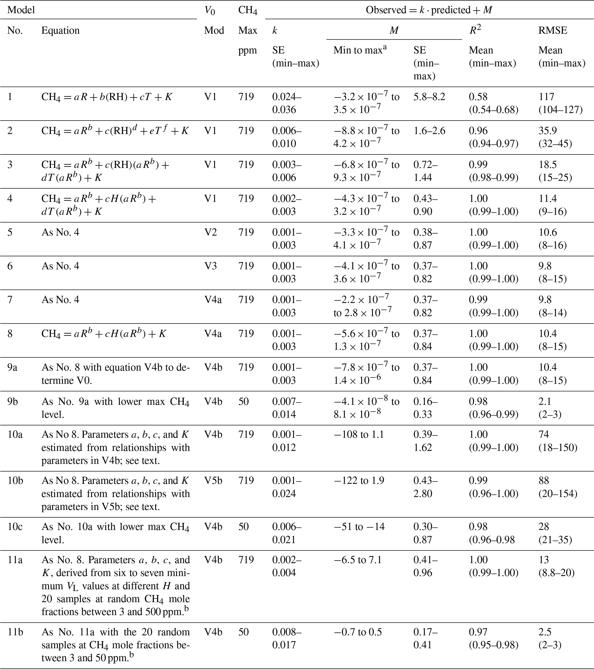
^a Minimum and maximum mean intercepts for the group of 20 sensors. The confidence interval around the mean intercept was ±1.1 ppm in Model 7 (having the lowest RMSE). ^b Monte Carlo simulations with 1000 runs generating random data subsets used for deriving the model parameter ranges.

2.3.2 Simplified calibration approaches without dedicated calibration experiment data (Approaches II and III)

The model combinations from Steps 1 and 2 above that generated the best fit with the minimum number of parameters were selected for tests of two simplified calibration approaches. In Approach II we tested if model parameters in Step 2 can be predicted from parameters derived in Step 1, hypothesizing that the derived model parameters in both Step 1 and Step 2 reflect the sensor capacity to respond to CH₄ and humidity levels as well as the individual sensor offset. If correct, the parameters in Step 1 should be correlated with parameters in Step 2. If this correlation is strong enough, it may be possible to predict parameters in Step 2 from parameters in Step 1, which can be derived from measurements at background air concentrations under the natural variation in humidity (e.g., the diel variability), as a part of the regular measurements, preferentially using data when the atmospheric boundary layer is well mixed (e.g., windy conditions). Under such conditions atmospheric background CH₄ concentrations can be relatively accurately assumed. Hence this Approach II would not require access to sensor calibration chambers, nor expensive reference gas analyzers, which in turn would make sensor measurements available much more broadly. To test this approach, we searched for the best possible regression equations to predict Step 2 parameters from Step 1 parameters, and then we used these equations to estimate CH₄ mole fractions and compared this with the UGGA reference measurements.

In Approach III we evaluated if reasonable accurate Step 1 and 2 equations can be derived from the combination of (i) minimum background atmospheric level V_L at different humidity and (ii) a limited number of randomly collected independent manual flux chamber samples. If so, a few manual samples during the regular measurements could replace tedious dedicated calibration experiments. To test this approach the calibration data for each sensor were subsampled randomly and these random subset data were combined with the minimum V_L data to derive calibration parameters as done in Approach I. Using these parameters, the CH₄ mole fractions for all of the calibration data were estimated and compared with observed values. Monte Carlo simulations were run to test effects of the number of random reference samples (1–50) and the methane concentration ranges (3–500 or 3–50 ppm, respectively) in the subset data.

2.3.3 A low-cost Arduino-based CH₄–CO₂–RH–T logger

To facilitate use of the sensors and our results, we also gathered instructions for how to build a logger for CH₄, CO₂, RH, T measurements, using the CH₄ sensor tested here, and the Senseair K33 ELG CO₂–RH–T sensor described elsewhere (Bastviken et al., 2015), a supplementary DHT22 sensor for RH and T, an Arduino controller unit, and an Adafruit Arduino compatible logger shield with a real-time clock (input voltage 7–12 V; 10 bit resolution; Fig. 1). This development was based on sensor specifications and the open-source knowledge generously shared on the internet by the Arduino user community. The full description of this logger unit is found in the Supplement.

Figure 1 Photo of the CH₄–CO₂–RH–T logger described in the Supplement.

3 Results and discussion

The results of different Step 1 and Step 2 calibration equations are shown in Tables 1 and 2. The models including H were equal or superior to models using RH. This is reasonable because it is the absolute water molecule abundance that influences the sensor response. Hence, models using H were prioritized. In Approach I, several Step 1 models, including a constant minimum V_L, and power, linear, and Michaelis–Menten-based equations gave similar R² (0.85 to 0.9) and root-mean-square error (RMSE) when comparing predicted versus observed results (Table 1). The effect of T appeared negligible compared to H, which may be related to the built-in heating of the active sensor surface (280 mW; this heating was focused on a small part of the sensor, and no self-heating around sensors was detected). It is possible that the Michaelis–Menten equation is superior over the full theoretically possible H range. However, under our experiment conditions, covering normal field H levels, the combination of best fit and minimum number of parameters in Step 1 was found for a simple linear equation with H (Model V4 in Table 1), which was used for later tests of Approaches II and III.

The tests of different equations in Approach I, Step 2, showed that power relationships with H and T represented as interactions with the sensor response performed best (Table 2, Model ≥4). With the exception of Models 10a–c, all these models had in the regression of observed versus predicted a slope and intercept that were statistically indistinguishable from 1 and 0, respectively (p<0.05), and an R² of 0.98–1.00 (Table 2, Figs. 2, S1, and S2). Again, T had a marginal effect and H was clearly most important. Hence, while Model 7 including T in Table 2 had the lowest RMSE (9.8), Model 8 represented a good compromise between minimum number of parameters and low RMSE (10.4) and was used in Approaches II and III. The nonlinear response of the sensor yielded a stronger and more coherent response at low CH₄ levels, and a large part of the uncertainty was generated at the higher CH₄ levels in the studied range (Figs. 2, S1, and S2). Near the atmospheric background at 2 ppm, the confidence interval for individual sensor response was on the order of ±1.1 ppm (Model 7 having the lowest RMSE). Hence, the presented calibration equations have a limited accuracy in terms of absolute CH₄ mole fractions and are not optimized for high-precision measurements at atmospheric background levels (as shown by SE for the model intercept corresponding to 0.16–1 ppm; Table 2). However, high R² and low SE for the slope of several models indicate that the relative change of CH₄ levels over time, which is the core of flux chamber measurements, can be assessed efficiently with the sensors if calibrated properly (Table 2).

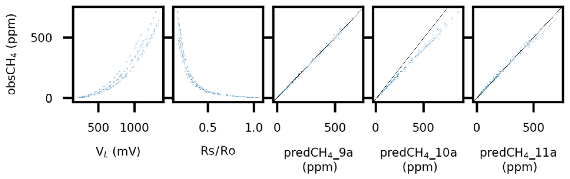
Figure 2 Sensor output voltage (V_L; mV), R_S∕R₀ ratio, and predicted CH₄ mixing ratio (predCH₄; ppm) using Models 9a, 10a, and 11a in Table 2, respectively, versus observed CH₄ mixing ratio (obsCH₄; ppm), for one of the studied sensors. See text for details and Figs. S1 and S2 in the Supplement for similar graphs regarding all sensors. Black diagonals represent 1:1 lines.

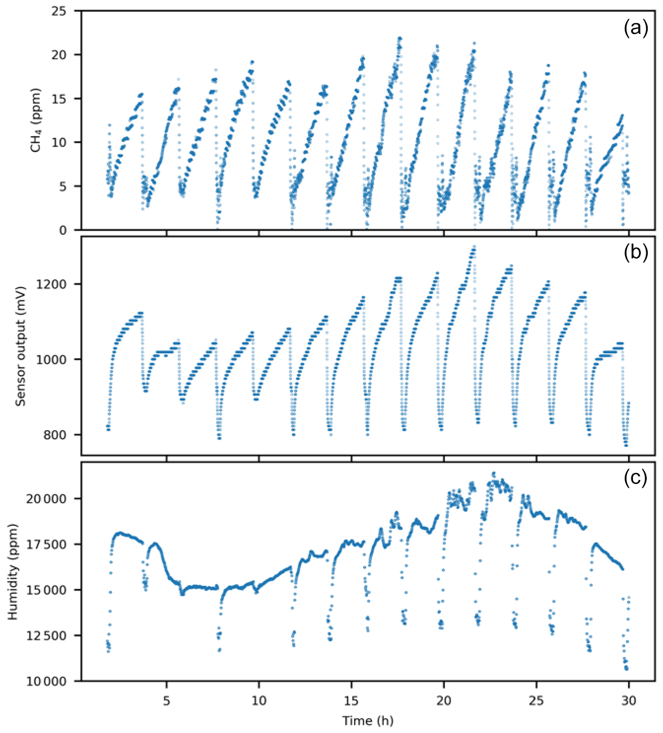
Figure 3 Real data from a flux chamber on a lake in June 2019 with 14 automated chamber open–closure cycles over 30 h. Each cycle included a closed phase during which CH₄ increased in the chamber over time, followed by opening the chamber for flushing to background levels before starting the next cycle by closing the chamber. Panels show (a) calibrated CH₄ mole fractions based on this study, (b) untreated sensor output signal, and (c) absolute humidity.

Approach II, deriving all calibration equations from a small set of minimum V_L values using Models V4 or V5 (Table 1) and 10a–c (Table 2), generated substantially greater RMSE. Most of this RMSE change was due to less accurate prediction of the intercept. The R² and slope standard error range remained similar to the other models (Table 2), but the actual slope values could deviate substantially from 1 and varied considerably among sensors (in contrast to the models for all other approaches always having slopes close to 1 and similar among sensors; Figs. 2, S1, and S2). Thereby, Approach II could lead to a large bias in absolute mole fractions. This crude generation of calibration equations may be adequate primarily for assessing relative change over time measured by the same sensor, and cross comparisons among sensors should be avoided when using this approach. Examples of equations for the parameter estimation in Approach II are provided in Table S1 in the Supplement. Applying Approach II to a smaller concentration range yielded a considerably lower RMSE (Table 2, Model 10c).

Approach III (Model 11a and 11b in Table 2) showed that as few as 10–20 reference samples, collected at random occasions during actual measurements, could substantially reduce the RMSE of the calibration models, reaching close to the lowest levels based on the 619–930 measurements and the full range up to 719 ppm in Approach I (Table 2 Model 11a; Fig. S3). The concentrations of the reference samples did not appear important for the RMSE within a given specific data range. However, simulations using data for CH₄ mole fractions below 50 ppm only generated much lower RMSE than using all data (Table 2, Model 11b). This supports the conclusion that the sensors are more sensitive and give a stronger relative response in the low part of the studied concentration range.

An overview of approaches to derive calibration models for this type is shown in Table S2. The challenges found regarding monitoring of background atmospheric levels were confirmed by our study, while use for relative changes of greater magnitudes in flux chambers appears promising based on our results, also with a simplified calibration (Approach III). As a general note for all approaches when used under variable environmental conditions, the best precision may be achieved by using absolute partial pressure units for both CH₄ and humidity, thereby compensating for variability in atmospheric pressure. In addition, for use above the maximum absolute humidity in this study, extra care is advised to check sensor capacity and behavior. An example of real field data is provided in Fig. 3. This example illustrates that the direct sensor response is heavily influenced by humidity and that the calibration equations shown in Tables 1 and 2 are needed to reveal the CH₄ part of the sensor signal. Further, Fig. 3 illustrates that sensors can be highly useful in very variable environments with rapid changes in humidity and when using data loggers with 10 bit resolution only. Optimal calibration procedures in stable environments and with higher logger resolution would likely indicate better sensor performance, while we deliberately focused on calibration procedures closely linked to field use with inexpensive equipment to provide information of relevance for as many conditions as possible.

Long-term stability of the sensors was not addressed here but is important for environmental use. Other studies of the same type of sensors show promising results. For example, van den Bossche et al. (2017) found no drift over 31 d. Eugster et al. (2020) using the similar Figaro TGS 2600 sensor for outdoor measurements over 7 years concluded that the drift was on the order of 4–6 ppb yr⁻¹. This suggests that the sensor drift is modest even when exposed to variable weather over long time. However, it is possible that the drift can be faster under some conditions, and regular drift checks are therefore advised.

4 Conclusions

The main conclusions can be summarized as follows.

• The tested CH₄ sensors are suitable for use in flux chamber applications if there are simultaneous measurements of relative humidity and temperature.

• Sensor-specific calibration is required.

• Occasional independent reference samples during regular measurements can be an alternative to designated calibration experiments. Background atmospheric levels in combination on the order of 10–20 in situ reference samples at other CH₄ levels can yield rather accurate calibration models.

• For the highest accuracy regarding absolute CH₄ concentrations, careful designated calibration experiments covering relevant environmental conditions are needed.

• These results, together with the increased accessibility of low-cost sensors and data logger systems (one example described in the Supplement), open supplementary paths toward improved capacity for greenhouse gas measurements in both nature and society.