the Creative Commons Attribution 4.0 License.
the Creative Commons Attribution 4.0 License.
 | 23 Jul 2020
The Southern Annular Mode (SAM) influences phytoplankton communities in the seasonal ice zone of the Southern Ocean
Bruce L. Greaves
Andrew T. Davidson
Alexander D. Fraser
John P. McKinlay
Andrew Martin
Andrew McMinn
Simon W. Wright
Ozone depletion and climate change are causing the Southern Annular Mode (SAM) to become increasingly positive, driving stronger winds southward in the Southern Ocean (SO), with likely effects on phytoplankton habitat due to possible changes in ocean mixing, nutrient upwelling, and sea ice characteristics. This study examined the effect of the SAM and 12 other environmental variables on the abundance of siliceous and calcareous phytoplankton in the seasonal ice zone (SIZ) of the SO. A total of 52 surface-water samples were collected during repeat resupply voyages between Hobart, Australia, and Dumont d'Urville, Antarctica, centred around longitude 142∘ E, over 11 consecutive austral spring–summer seasons (2002–2012), and spanning 131 d in the spring–summer from 20 October to 28 February. A total of 22 taxa groups, comprised of individual species, groups of species, genera, or higher taxonomic groups, were analysed using CAP analysis (constrained analysis of principal coordinates), cluster analysis, and correlation. Overall, satellite-derived estimates of total chlorophyll and measured depletion of macronutrients both indicated a more positive SAM was associated with greater productivity in the SIZ. The greatest effect of the SAM on phytoplankton communities was the average value of the SAM across 57 d in the previous austral autumn centred around 11 March, which explained 13.3 % of the variance in community composition in the following spring–summer. This autumn SAM index was significantly correlated pair-wise (p<0.05) with the relative abundance of 12 of the 22 taxa groups resolved. A more positive SAM favoured increases in the relative abundance of large Chaetoceros spp. that predominated later in the spring–summer and reductions in small diatom taxa and siliceous and calcareous flagellates that predominated earlier in the spring–summer. Individual species belonging to the abundant Fragilariopsis genera responded differently to the SAM, indicating the importance of species-level observation in detecting SAM-induced changes in phytoplankton communities. The day through the spring–summer on which a sample was collected explained a significant and larger proportion (15.4 %) of the variance in the phytoplankton community composition than the SAM, yet this covariate was a proxy for such environmental factors as ice cover and sea surface temperature, factors that are regarded as drivers of the extreme seasonal variability in phytoplankton communities in Antarctic waters. The impacts of SAM on phytoplankton, which are the pasture of the SO and principal energy source for Antarctic life, would have ramifications for both carbon export and food availability for higher trophic levels in the SIZ of the SO.
- Article
(9105 KB) - Full-text XML
-
Supplement
(1738 KB) - BibTeX
- EndNote


Phytoplankton are the primary producers that feed almost all life in the oceans. In the Southern Ocean (SO), defined as the southern portions of the Atlantic Ocean, Indian Ocean, and Pacific Ocean south of 60∘ S (Arndt et al., 2013), spring–summer phytoplankton blooms in the seasonal ice zone (SIZ) feed swarms of krill which, in turn, are key food for sea-birds, fish, whales, and almost all Antarctic life (Smetacek, 2008; Cavicchioli et al., 2019). Phytoplankton also play a critical role in ameliorating global climate change by capturing carbon through photosynthesis. Around one-third of the carbon fixed by phytoplankton in SIZ of the SO sinks out of the surface ocean (Henson et al., 2015), more than the global ocean average of around 20 % (Boyd and Trull, 2007; Ciais et al., 2013; Henson et al., 2015). With total productivity within the SIZ of the SO estimated at 68–107 Tg C yr−1 (Arrigo et al., 2008), this equates to 23–36 Tg C yr−1, around 0.2 %–0.3 % of the estimated annual global marine biota export of 13 Pg (Ciais et al., 2013), being sequestered to the deeper ocean for climatically significant periods of time, likely hundreds to thousands of years (Lampitt and Antia, 1997). Even so, the SIZ of the SO shows a net release of CO2 from the ocean to the atmosphere due to off-gassing of carbon-rich deep-ocean water upwelling at the Antarctic Divergence (Takahashi et al., 2009). Thus any changes in the composition and abundance of phytoplankton in the SIZ are likely to influence both the trophodynamics of the SO and the contribution of the region to oceanic–atmospheric carbon flux.
Global standing stocks of phytoplankton are estimated to have been declining by as much as 1 % per year, a decline largely attributed to rising surface ocean temperature (Boyce et al., 2010, 2011; Mackas, 2011). Furthermore, global phytoplankton productivity is predicted to drop by as much as 9 % from the years 1990 to 2090 (RCP8.5, “business as usual”), with a decline across most of the Earth’s ocean area (Bopp et al., 2013). In contrast, higher latitudes, including the SIZ of the SO, are predicted to experience an increase in phytoplankton productivity due to changes to seasonal ice extent and duration (Parkinson, 2019; Turner et al., 2013) and/or increased upwelling of nutrient-rich deep ocean water at the Antarctic Divergence (Steinacher et al., 2010; Bopp et al., 2013; Carranza and Gille, 2015).
1.1 Importance of the SIZ phytoplankton bloom
The Antarctic SIZ is one of the most productive parts of the SO (Carranza and Gille, 2015). It is also a significant component of the global carbon cycle by virtue of both carbon sequestration by phytoplankton (Henson et al., 2015) as well as upwelling and off-gassing of carbon-rich deep ocean water (Takahashi et al., 2009). It is one of the largest and most variable biomes on Earth, with sea ice extent varying from around 20 million km2 during winter to only 4 million km2 in summer (Turner et al., 2015; Massom and Stammerjohn, 2010; Parkinson, 2019). The most macronutrient-rich surface waters of the SIZ occur over the Antarctic Divergence, a circumpolar region of the SO located at around 63∘ S where carbon- and nutrient-rich water upwells to the surface, supplying the nutrients that drive much of the phytoplankton production in the SO (Lovenduski and Gruber, 2005; Carranza and Gille, 2015).
In winter, phytoplankton growth is limited by light availability and temperature. In spring and summer, phytoplankton can proliferate in the high-light, high-nutrient waters that trail the southward retreat of sea ice (Fig. 1a, b) (Wilson et al., 1986; Smetacek and Nicol, 2005; Lannuzel et al., 2007; Saenz and Arrigo, 2014; Rigual-Hernández et al., 2015). The SIZ supports high phytoplankton standing stocks and productivity, and phytoplankton abundance in blooms can double every few days (Wilson et al., 1986; Sarthou et al., 2005). Wind speed is a primary determinant of phytoplankton bloom development in the SIZ, with calmer conditions fostering shallow mixed depths that maintain phytoplankton cells in a high-light environment and maximise productivity (Savidge et al., 1996; Fitch and Moore, 2007). Phytoplankton populations are characterised by large-scale spatial and temporal variability (Martin et al., 2012) with only 17 %–24 % of ice edge waters experiencing phytoplankton blooms in any spring–summer period (Fitch and Moore, 2007).
1.2 The Southern Annular Mode
The Southern Annular Mode (SAM), which is also variously also called the High-Latitude Mode and the Antarctic Oscillation, is well-represented by two alternative definitions: (a) the normalised zonal mean sea-level pressure at 40∘ S minus that at 65∘ S (Gong and Wang, 1999; Marshall, 2003) or (b) the principal mode of atmospheric circulation at high latitudes of the Southern Hemisphere. The SAM reflects the position and intensity of a zonally symmetric structure of atmospheric circulation in the Southern Hemisphere, circling the Earth (annular) at around 50∘ S, and it has been defined as the alternating pattern of strengthening and weakening westerly winds in conjunction with high- to low-pressure bands (Ho et al., 2012). Variation in the SAM typically describes around 35 % of total Southern Hemisphere climate variability (Marshall, 2007), and the SAM is currently the dominant large-scale mode through which climate change is expressed at SO latitudes (Thompson and Solomon, 2002; Lenton and Matear, 2007; Lovenduski et al., 2007; Swart et al., 2015). Between 1979 and 2017 the value of daily SAM averaged 0.04 index points, ranged from −5.13 to 4.64, and had a standard deviation of 1.38 (after data by NOAA, 2017). Average monthly SAM varied from −2.7 to 2.5 index points over the 11 years studied (Fig. 1c).
There was a trend toward more positive SAM from 1979 to 2017 of 0.011 index points per year (NOAA, 2017), attributed to both ozone depletion (Thompson and Solomon, 2002; Arblaster and Meehl, 2006; Gillett and Fyfe, 2013; Jones et al., 2016) and increasing atmospheric greenhouse gas concentrations (Thompson et al., 2011). The long-term average SAM is now at its most positive level for at least the past 1000 years (Abram et al., 2014). Continuing increases in atmospheric greenhouse gases are expected to drive a further positive increase in the SAM in all seasons (Arblaster and Meehl, 2006; Swart and Fyfe, 2012; Gillett and Fyfe, 2013), despite the expected recovery in stratospheric ozone concentrations to pre-ozone hole values by around 2065 (Son et al., 2009; Schiermeier, 2009; Thompson et al., 2011; Solomon et al., 2016).
A more positive SAM indicates the occurrence of a strengthening circumpolar vortex (Marshall, 2003; Ho et al., 2012), leading to stronger westerly winds and increased storminess at high latitudes (Hall and Visbeck, 2002; Kwok and Comiso, 2002; Lovenduski and Gruber, 2005; Arblaster and Meehl, 2006). These changes are particularly marked south of 60∘ S in the atmospheric Southern Circumpolar Trough (Hines et al., 2000; Mackintosh et al., 2017), a region characterised by strong winds with variable direction (Taljaard, 1967). Stronger winds associated with more positive SAM may result in increased transport of surface water northward from the Antarctic Divergence by Ekman drift (Lovenduski and Gruber, 2005; DiFiore et al., 2006), potentially driving increased upwelling of nutrient- and carbon-rich deep ocean water at the Antarctic Divergence (Hall and Visbeck, 2002). More positive SAM is also associated with reduced near-surface air temperature over the SIZ due to an increased frequency of strong southerly winds and increased cloud cover (Lefebvre et al., 2004; Sen Gupta and England, 2006; Marshall, 2007). Sea ice extent around the Antarctic continent shows zonal relationships with the SAM, with positive relationships between the SAM and sea ice extent in the western Pacific and Indian sectors of the SO and negative or non-existent relationships in other sectors (Kohyama and Hartmann, 2016). Wind also affects the nature of the sea ice, breaking up floes via wave interactions, increasing flooding, and changing pack ice density (compressing or opening up the pack) and contributing to ice formation by generating frazil ice (Massom and Stammerjohn, 2010; Squire, 2020). Lower sea-surface temperatures have been observed to lag positive SAM events by 1 to 4 months (Lefebvre et al., 2004; Meredith et al., 2008), and changes in the SAM may take weeks to months to be manifested in phytoplankton communities (Sen Gupta and England, 2006; Meredith et al., 2008). Extreme SAM events might also impact phytoplankton communities for multiple years (Ottersen et al., 2001).
By modulating upwelling, ocean mixed depth, air temperature, and sea ice characteristics and duration, it is likely that a more positive SAM will affect the composition and abundance of phytoplankton in the SIZ of the SO. Lovenduski and Gruber (2005) predicted that more positive SAM would support higher phytoplankton productivity, and subsequent analyses by Arrigo et al. (2008), Boyce et al. (2010), and Soppa et al. (2016) have confirmed a positive relationship between the SAM and phytoplankton standing stocks and productivity south of 60∘ S in the SIZ.
1.3 The hypothesis
Based on the predicted and observed positive relationships between the SAM and phytoplankton standing stocks and productivity in the SIZ of the SO, we hypothesised that changes in the SAM could also elicit changes in the composition of the phytoplankton community. To test this hypothesis, we conducted a scanning electron microscopic survey of hard-shelled phytoplankton in surface waters of the Antarctic SIZ using samples collected between October and February each spring–summer over 11 consecutive years (2002–2003 to 2012–2013). We then related the composition of these communities to environmental variables including the SAM.
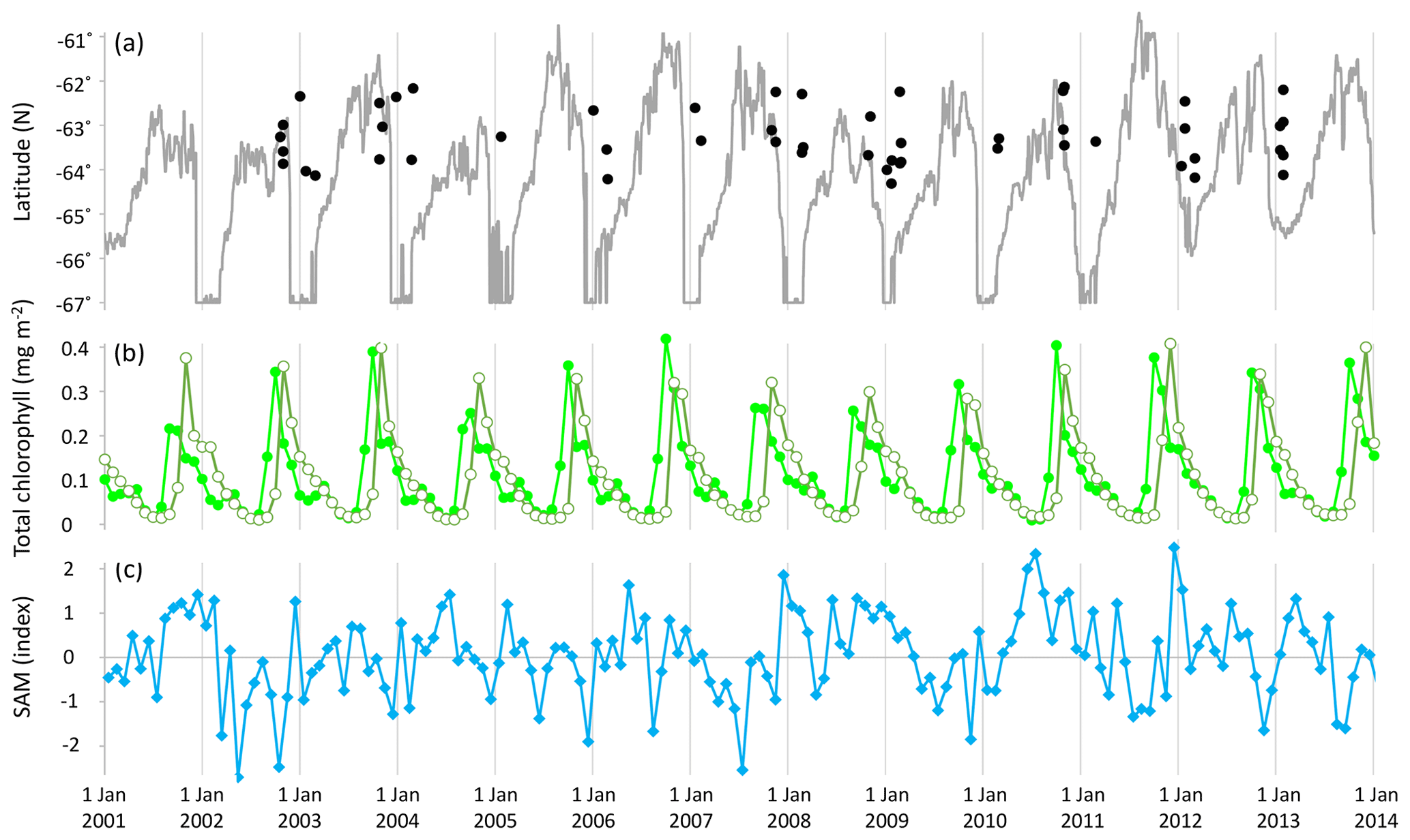
Figure 1(a) Latitude and timing of samples (black filled circles) and sea ice extent at 143∘ E (grey solid line); (b) monthly total chlorophyll (Acker and Leptoukh, 2007; GMAO, 2017) across the sampled area (longitude 135.7–147.8∘ E): northern extent (latitude −62∘ N, light green solid circles) and southern extent (latitude −64.5∘ N, olive-green open circles); and (c) monthly average of daily SAM (NOAA, 2017).

Figure 2Example of phytoplankton identification on a single SEM image, representing 0.0348 mL of seawater. Overlying letters are taxa codes for individual phytoplankton taxa considered in the analysis (listed in Table 3); codes in parenthesis are rare taxa (see text). Inset: sampling area in relation to southern Australia and the Antarctic coastline, with sample locations indicated as open circles.
A total of 52 surface-water samples were collected from the seasonal ice zone (SIZ) of the Southern Ocean (SO) across 11 consecutive austral spring–summers from 2002–2003 to 2012–2013. The samples were collected aboard the French re-supply vessel MV L'Astrolabe during resupply voyages between Hobart, Australia, and Dumont d'Urville, Antarctica, between 20 October and 28 February. Most samples were collected from ice-free water, although some were collected south of the receding ice edge (Fig. 1a).
The sampled area was in the Indian sector of the SO, spanning 270 km of latitude between 62 and 64.5∘ S and 625 km of longitude between 136 and 148∘ E (Fig. 2 inset). The area lies >100 km north of the Antarctic continental shelf break, in waters >3000 m depth.
Samples were obtained from the clean seawater line of the re-supply vessel from around 3 m depth. Each sample represented 250 mL of seawater filtered through a 25 mm diameter polycarbonate-membrane filter with 0.8 µm pores (Poretics). The filter was then rinsed with two additions of approximately 2 mL of Milli-Q water to remove salt, then air dried and stored in a sealed container containing silica gel desiccant. Samples were prepared for scanning electron microscope (SEM) survey by mounting each filter onto a metal stub and sputter coating with 15 nm gold or platinum. Only organisms possessing hard siliceous or calcareous shells were sufficiently well preserved through the sample preparation technique that they could be identified by SEM, and these included diatoms, coccolithophores, silicoflagellates, Pterosperma, Parmales, radiolarians, and armoured dinoflagellates.
2.1 Phytoplankton relative abundance
The composition of the phytoplankton community of each sample was determined from ×400 magnification images captured using a JEOL JSM 840 Field Emission SEM. Cell numbers for each phytoplankton taxon were counted in a random selection of captured images taken of each sample. Each captured image (Fig. 2) represented an area of 301 µm × 227 µm (area 0.068 mm2) of each sample filter, which was captured at a resolution of 8.5 pixels per micrometre. A minimum of three SEM images were assessed for each sample, with more images assessed when cell densities were lower – individual images were considered as incremental increases in the area of a sample covered and not sampling replicates. On average, 387 cells were counted for each sample. Taxa were classified with the aid of Scott and Marchant (2005), Tomas (1997), and expert opinion. Cell counts per sample were converted to volume-specific abundances (cells per mL) by dividing total counts by the number of images assessed multiplied by 0.0348 mL of seawater represented by each captured image.
A total of 48 phytoplankton taxa were identified, many to species level. Because the diatoms Fragilariopsis curta and F. cylindrus could not be reliably discriminated at the microscope resolution employed, they were pooled into a single taxa group. Other taxa were also grouped, namely Nitzschia acicularis with N. decipiens to a single group, and discoid centric diatoms of the genera Thalassiosira, Actinocyclus, and Porosira to another. Rare species, with maximum relative abundance <2 %, were removed from the data prior to analysis as they were not considered to be sufficiently abundant to warrant further analysis (Webb and Bryson, 1972; Taylor and Sjunneskog, 2002; Świło et al., 2016). After pooling taxa and deleting rare taxa, 22 taxa and taxonomic-groups (species, groups of species, and families) remained to describe the composition of the phytoplankton community. A total of 19 499 phytoplankton organisms were identified and counted: 18 878 diatoms, 322 Parmales, 173 coccolithophores, 81 silicoflagellates, and 45 Petasaria.
Phytoplankton abundance data were converted to relative abundance by dividing each value by the total abundance of the 22 taxa groups in the sample. This was to alleviate any variation among samples resulting from dilution, a phenomenon whereby the abundance of cells in surface waters can be reduced in a matter of hours by an abrupt increase in wind speed and associated increase in the mixed layer depth (Carranza and Gille, 2015), diluting near-surface cells into a greater water volume. However, relative abundance has the disadvantage that blooming of one species will cause a reduction in relative abundance of other present species, when their absolute abundances may not have changed.
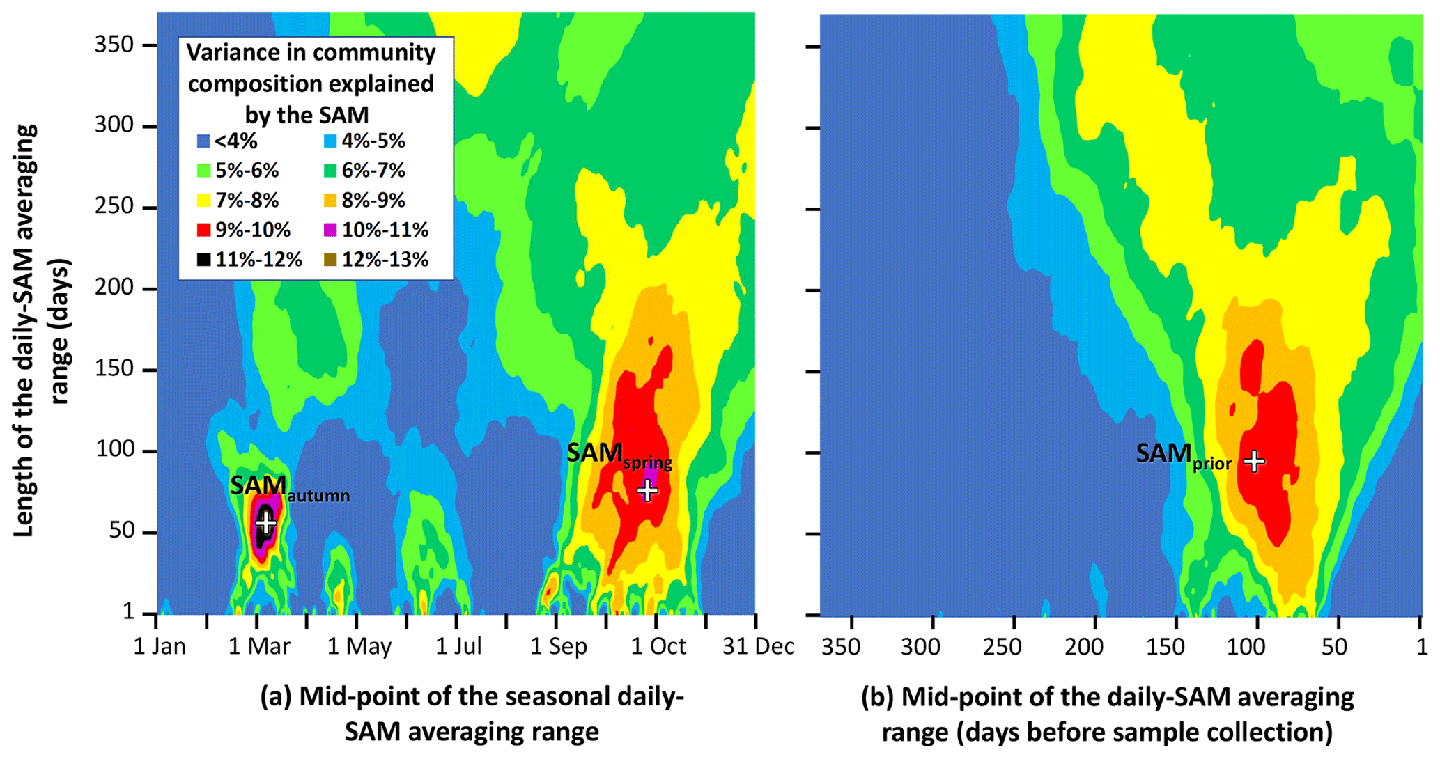
Figure 3Variance in phytoplankton community composition explained by the SAM, versus timing and length of the averaged range of daily SAM values. Response surfaces relate the fraction of total variance in phytoplankton community composition attributable to the SAM, versus the number of days in the range of the averaged daily SAM (vertical axis) and the timing of the centre of the range of the averaged daily SAM (horizontal axis). The horizontal axis is expressed as (a) the time through the calendar year of the middle of the range, and (b) the number of days before a sample was collected, to the middle of the range. Three obvious maxima are identified with crosses (SAMautumn, SAMspring, and SAMprior).
2.2 Environmental covariates
Phytoplankton abundances were related to a range of environmental covariates available at the time of sampling. These included the SAM, sea surface temperature (SST), salinity (S), time since sea ice cover (DSSI, defined below), minimum latitude of sea ice in the preceding winter, latitude and longitude of sample collection (LATS and LONGE respectively), the days since 1st October that a sample was collected (D), the year of sampling (Y, being the year that each spring–summer sampling season began), the time of day that a sample was collected, and satellite-derived total chlorophyll content. Macronutrient concentrations, phosphate (PO4), silicate (SiO4), and nitrate + nitrite (hereafter nitrate, NOx) were included as indicators of nutrient drawdown as a proxy for phytoplankton productivity (Arrigo et al., 1999).
We obtained daily estimates of the SAM from the US NWS Climate Prediction Center (NOAA, 2017). This dataset uses the principal component method definition of the SAM (Mo, 2000), rather than the simple zonal-mean normalised pressure difference technique (Gong and Wang, 1999). We used these estimates principally because daily values were readily available; other available estimates were largely seasonal averages only (Ho et al., 2012). Water samples for dissolved macronutrients were collected, frozen on the ship, and later analysed at the Commonwealth Scientific and Industrial Research Organisation in Hobart, Australia, using standard spectrophotometric methods (Hydes et al., 2010). The variable DSSI was defined as the time since sea ice had melted to 20 % cover, after Wright et al. (2010), as determined from daily Special Sensor Microwave/Imager (SSM/I) sea ice concentration data distributed by the University of Hamburg (Spreen et al., 2008). Total chlorophyll content was estimated for each sample location by estimating the total chlorophyll content over a 20 km × 20 km area centred at each sample location, for all available times from 31 August to 1 May in the year of sampling (monthly observations) (Acker and Leptoukh, 2007; GMAO, 2017), and interpolating between observations to estimate total chlorophyll content on the date sampled (some examples are reproduced in Fig. S3). By this method total chlorophyll was estimated for 49 of the 52 samples, the remainder of samples having a paucity of data which precluded estimation.
2.3 Statistical analysis
Three statistical analyses were undertaken to explore the hypothesis: (i) constrained analysis of principal coordinates (CAP, Anderson and Willis, 2003, also known as distance-based redundancy analysis, Legendre and Anderson, 1999) was used to estimate the influence of multiple environmental covariates in simultaneously explaining community composition; (ii) clustering techniques were used to explore similarities in phytoplankton community composition among samples, independently of environmental information, to define significantly different groups of samples with similar phytoplankton community composition; and (iii) correlation analysis was used to support observed relationships between phytoplankton community composition and environmental covariates.
For CAP and cluster analysis, relative abundance data were square-root-transformed to reduce possible dominance of the analysis by a few abundant taxa. The Bray–Curtis dissimilarity index (Bray and Curtis, 1957) was used to calculate the resemblance of samples based on their community structure. The advantage of this index for the cell count data was that similarity among samples was not strongly affected by the absence of taxa.
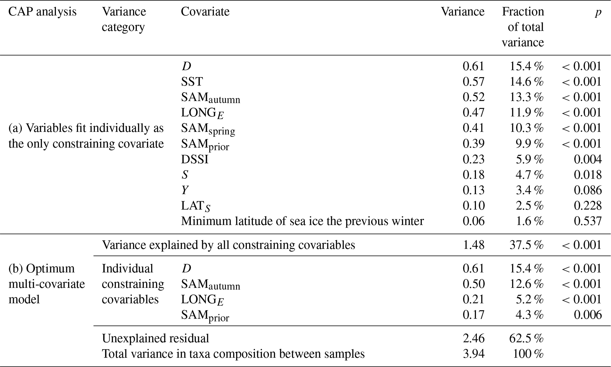
Table 1Variance in the community composition of 22 phytoplankton taxa groups attributable to constraining environmental covariables in the CAP analysis.
CAP was applied to the Bray–Curtis resemblance matrix to partition total variance in community composition into unconstrained and constrained components, with the latter representing the variation due to the environmental covariates. CAP is an example of a constrained ordination method in which the typical sample–species matrix of abundances (as used in redundancy analysis) is replaced with a symmetric matrix of pairwise sample similarities. The advantage of this distance-based approach to redundancy analysis is that any ecologically relevant distance measure may be used; here we use the Bray–Curtis metric because it discounts joint absences between samples when determining similarity. A forward selection strategy was used to choose the optimum model containing the minimum subset of constraints required to explain the most variation in phytoplankton community structure (Legendre et al., 2011). Linear projections of significant covariates were plotted as arrows in the ordination diagram, indicating the direction and magnitude of environmental gradients that were correlated with changes in the phytoplankton community (Davidson et al., 2016). The variance in phytoplankton community structure (as determined from the ordination) explained by each environmental covariate was calculated according to the procedure outlined in Ter Braak and Verdonschot (1995) and attributed to Dargie (1984). Taxa were added to the CAP plots as weighted site averages for each species, thereby indicating the relative influence of the fitted environmental constraints on each phytoplankton taxa group.
Hierarchical agglomerative clustering based on average linkage was performed on the Bray–Curtis resemblance matrix. Significant differences among sample clusters were determined according to the similarity profile (SIMPROF) permutation method of Clarke et al. (2008), based on α=0.05 and 1000 permutations. Clustering can identify the presence of significant differences between the community composition of the samples, but clustering cannot identify an effect of the SAM, at least not directly, since environmental covariates are not included in the cluster analysis.
Pair-wise correlation analyses were performed using Pearson's correlation coefficient r to explore the relationships among environmental variables, and between these environmental variables and the relative abundances of phytoplankton taxa (Rodgers and Nicewander, 1988). Given the large number of pair-wise correlations considered, we applied a Bonferroni correction to give consideration to the family-wise error rate by setting alpha, which is usually α=0.05 (Gibbons and Pratt, 1975; Cohen, 1990), to α∕m where m is the total number of correlations considered. Recognising that α∕m may be conservative (Nakagawa, 2004), we indicated when calculated correlations were significant at both α<0.05 and at Bonferroni-corrected .
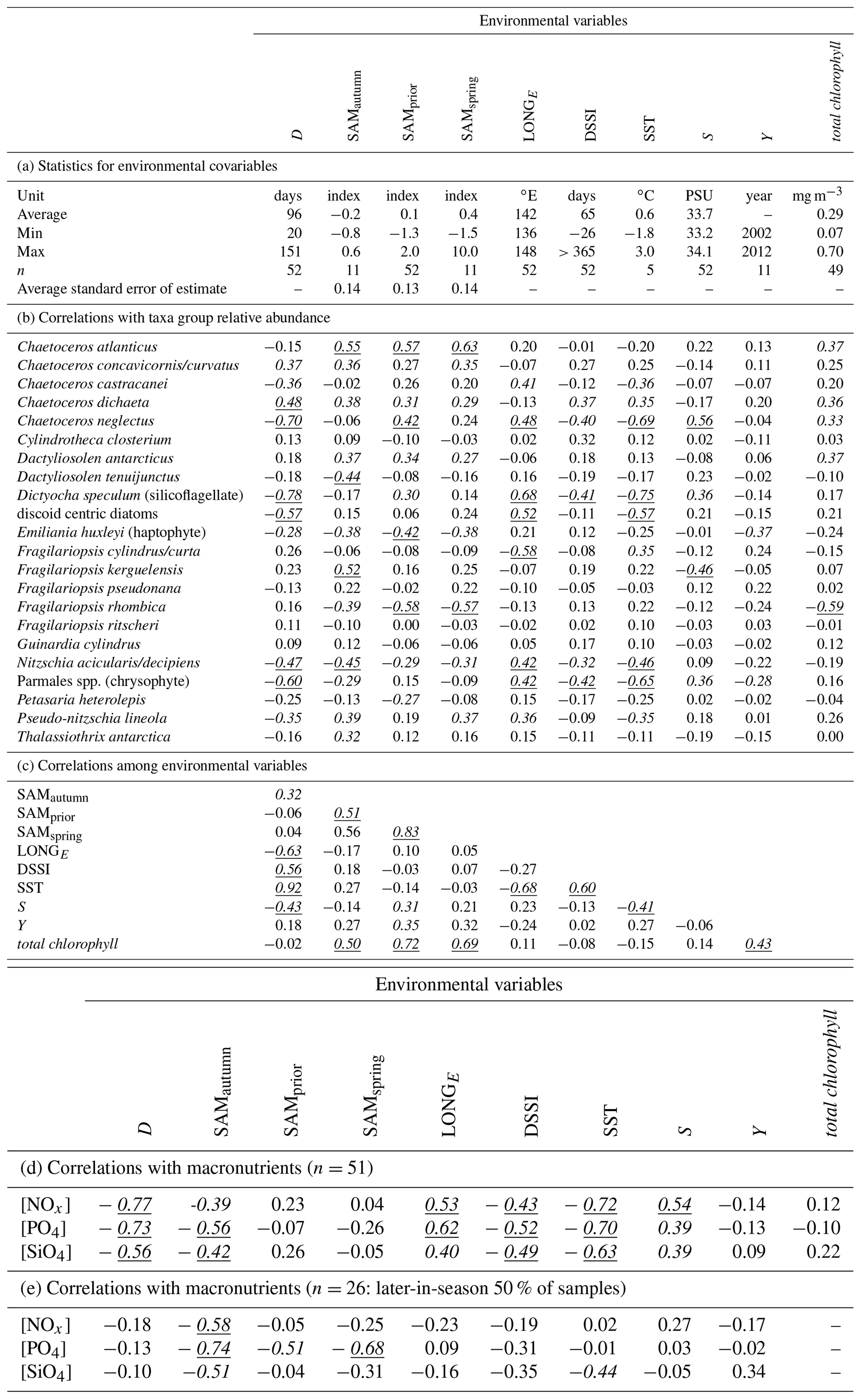
Table 2(a) Summary statistics for environmental variables; (b) correlations between taxa group relative abundances and environmental variables; (c) correlations among environmental variables; (d) correlations between macronutrient concentrations and environmental variables; (e) as in (f) but involving only the 50 % of samples collected latest in the spring–summer. Correlations significant at α≤0.05 are in italic, and correlations significant after Bonferroni adjustment are also underlined ( for correlations among environmental variables, for correlations with taxa group relative abundance).
Response surfaces were used to display the variance explained from individual CAP analyses according to the number of days averaged, and the mid-point (or lagged mid-point) of the range of days averaged, for each aggregated SAM index. These allowed identification of maxima in correlation between the SAM and phytoplankton community structure. Response surfaces were derived by evaluating separate CAP analyses for each combination of (i) the temporal positioning of the daily-SAM averaging range and (ii) the length of the daily-SAM averaging range. In constructing the response surfaces, the range of the averaged daily SAM was centred on (i) each calendar day individually (1 January–31 December) through the year associated with each sample, and alternatively (ii) relative to the time of sampling and lagged from 1 to 365 d prior to each sample collection date, in 1 d increments. The length of the SAM averaging range was varied in 2 d increments from zero to plus and minus 182 d from the centre of the range. Similar response surfaces were constructed relating the correlation between the averaged daily SAM and (i) total chlorophyll and (ii) [PO4].
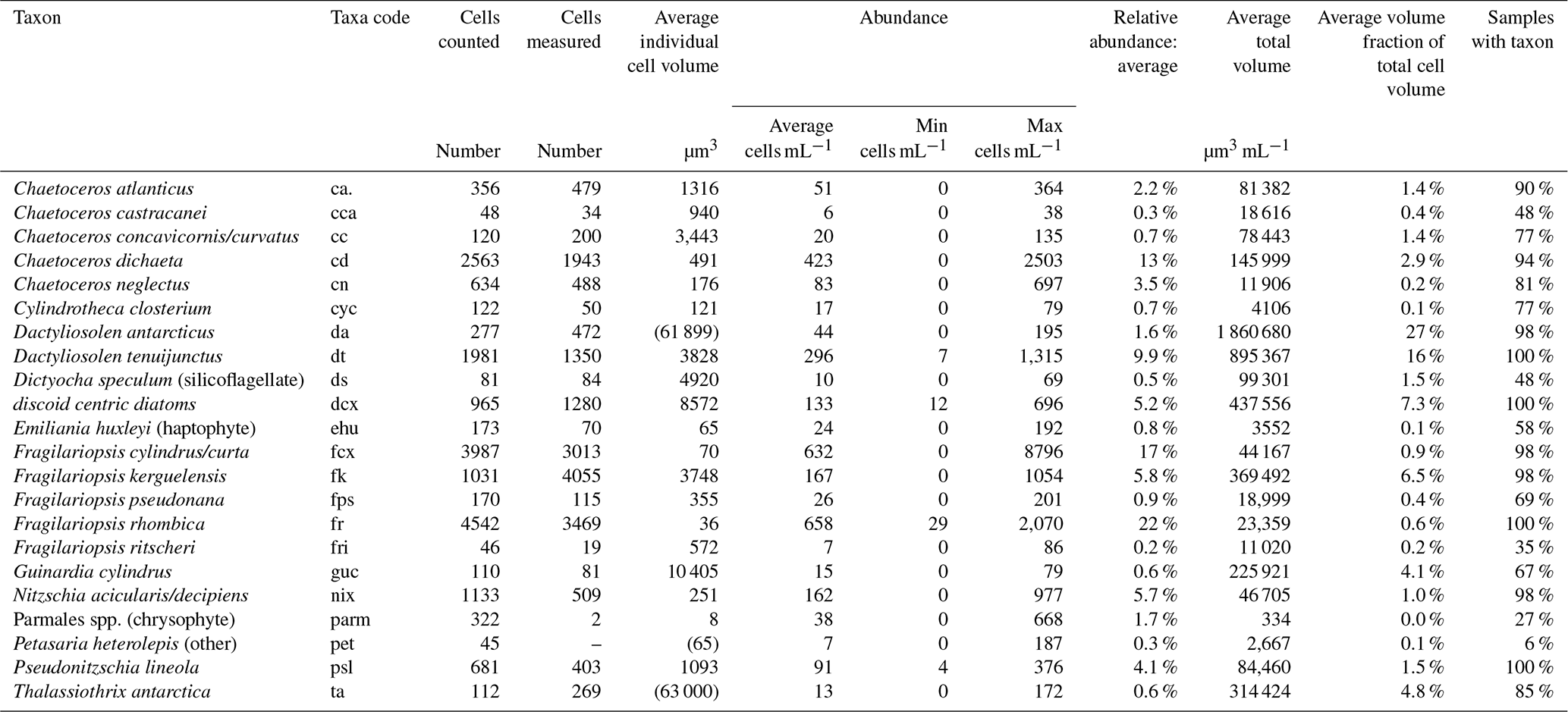
Table 3Identified taxa groups: taxa, taxa code, cells counted, cells measured, average individual cell volume, abundance (average, minimum, and maximum), average relative abundance, average total volume, average relative volume, and percentage of samples in which each taxa group was identified.
Data management and manipulation, summary statistics, correlation analyses, and scatter plots were undertaken in Microsoft Excel (2016) and R (R Core Team, 2016). Cluster analysis and SIMPROF were undertaken using the R package clustsig (Whitaker and Christman, 2014). CAP analyses were conducted using the capscale function in the R package vegan (Dixon, 2003).
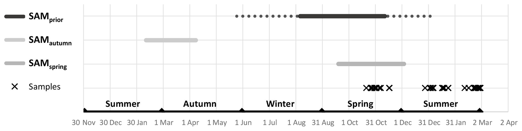
Figure 4Maxima of SAM influence on phytoplankton community composition. SAMprior was determined relative to sample collection: the depicted solid line represents the average temporal location of the 97 d period and the broken lines represent the earliest and latest extent of the range associated with the earliest and latest samples.
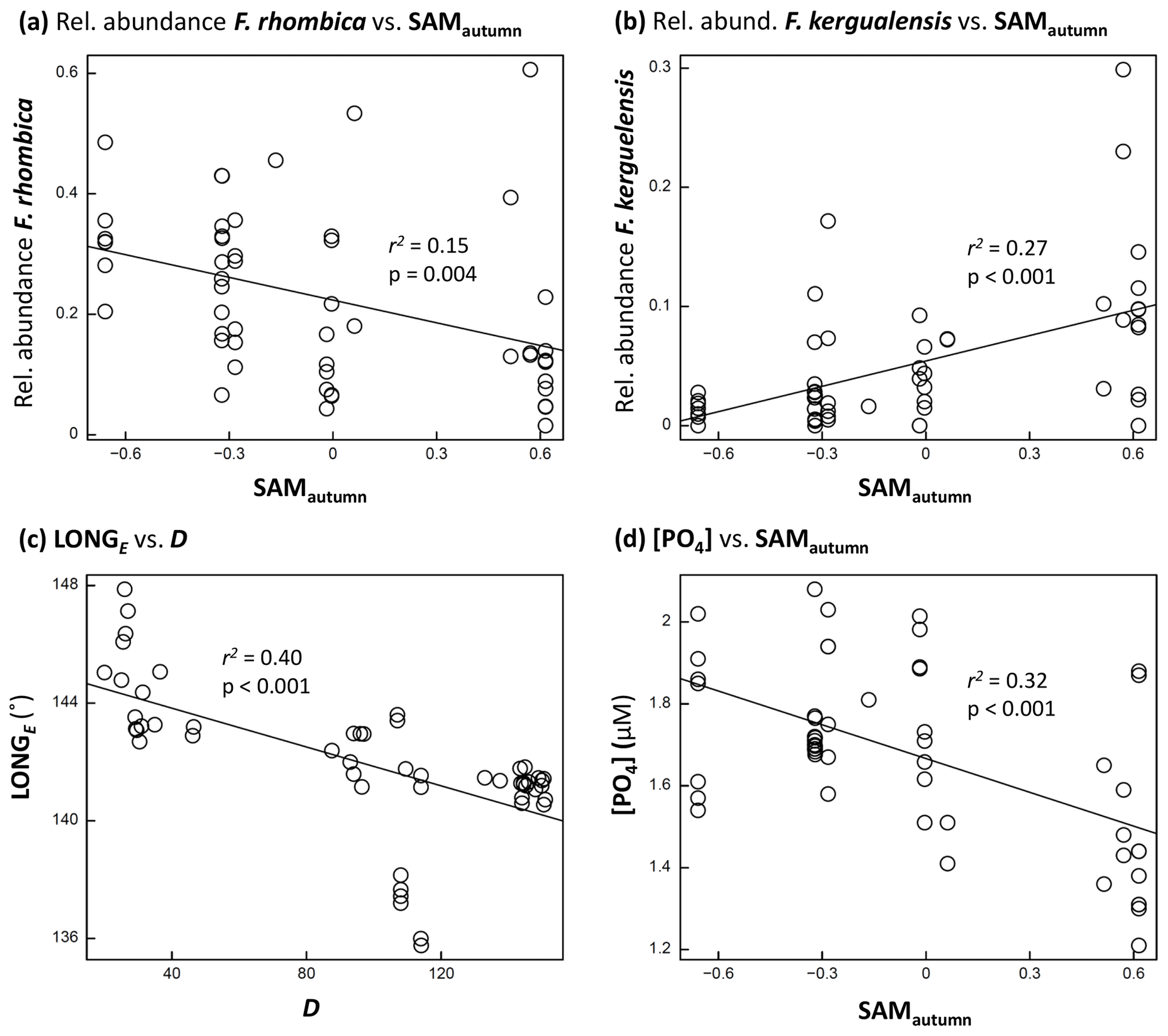
Figure 5Scatter-plots: (a, b) examples of phytoplankton taxon relative abundance versus SAMautumn; (c) LONGE of sample collection versus D; and (d) [PO4] versus SAMautumn. Each figure shows r2 and p associated with the relationship. A line of least-squares best fit is provided to give an indication of trend.
3.1 The influence of the SAM on phytoplankton community composition
CAP analysis and pairwise correlation analysis both indicated the presence of a relationship between the SAM and phytoplankton community composition. Clustering analysis showed there to be sufficient and systematic variation in phytoplankton community composition between samples that samples could be grouped.
Empirical identification of the time between variation in the SAM and the manifestation of this variation in the phytoplankton community structure revealed three maxima in phytoplankton community composition explained by the SAM. The first of the maxima was an autumn seasonal SAM index (SAMautumn), which was determined to be the average of 57 daily SAM estimates centred on the preceding 11 March (11 February–8 April). SAMautumn explained up to 13.3 % of the variance in phytoplankton community composition estimated through CAP analysis (Fig. 3a, Table 1a). The second of the maxima was a spring seasonal index (SAMspring), which was determined to be the average of 75 daily SAM estimates centred on 25 October (20 September–3 December). SAMspring explained up to 10.3 % of variance in phytoplankton community composition (Fig. 3a, Table 1a). Unlike the other maxima that were related to the time of year, the third of the maxima was timed relative to the date of sample collection for each sample and comprised the average of the 97 daily SAM estimates centred 102 d prior to each sample collection date. It explained 9.9 % of the variance in phytoplankton composition (SAMprior, Fig. 3b, Table 1a). Note that SAMprior and SAMspring temporally overlapped to varying extents across the 52 samples (Fig. 4) and so were not entirely independent covariates: for example, a sample collected in the summer had previous days contributing to both SAMprior and SAMspring.
The optimum CAP model contained four covariates that explained the variance in phytoplankton community composition among samples (Table 1b). While four CAP axes were statistically significant (p<0.05), the first two axes together explained a total of 31.1 % of the variance in phytoplankton community composition, and the third and fourth axes together only explained a further 6.4 % (not tabulated). Thus Fig. 6a illustrates most of the variance explained by the CAP analysis. SAMautumn explained the most variance in community composition (12.6 %) and SAMprior explained a further 4.3 % of variance (Table 1b). These two SAM indices were moderately and significantly positively correlated (r=0.51, Table 2c, p<0.001). Both showed similar negative correlations (Table 2b) with the relative abundances of the small diatoms Fragilariopsis rhombica (Fig. 5a) and Nitzschia acicularis/decipiens and the coccolithophorid Emiliana huxleyi, and similar positive correlations with the abundances of larger diatoms Chaetoceros atlanticus, Chaetoceros dichaeta, and Dactyliosolen antarcticus. A further six taxa showed a correlation with SAMautumn but not SAMprior, namely positive correlations with Chaetoceros concavicornis/curvatus, Fragilariopsis kerguelensis (Fig. 5b), Pseudo-nitzschia lineola, and Thalassiothrix antarctica, and negative correlations with Dactyliosolen tenuijunctus and the Parmales. Three taxa showed correlations with SAMprior but not SAMautumn, namely positive correlations with Chaetoceros neglectus and the silicoflagellate Dictyocha speculum, and a negative correlation with Petasaria heterolepis.
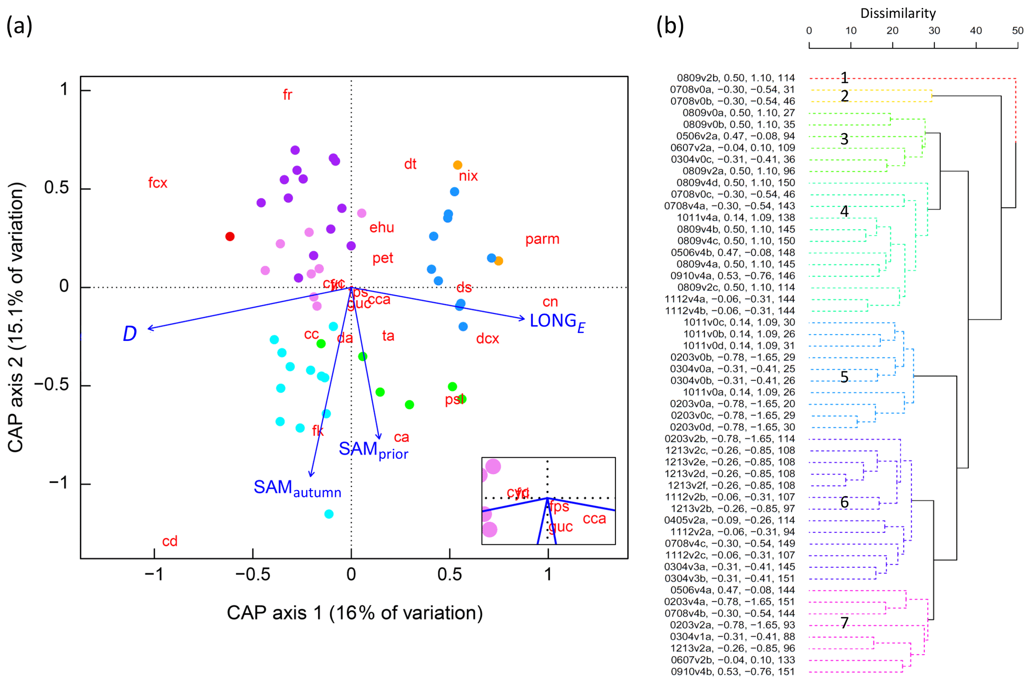
Figure 6(a) CAP analysis of phytoplankton community composition. Dots represent individual samples, with colours corresponding to significant clusters (Fig. 6b). The 22 phytoplankton taxa/groups are overlain as weighted averages of their sample scores (red abbreviations, after Fig. 2) with positions plotted with a 3-times-larger distance from the origin to more easily visualise their relationships with constraining environmental variables. Linear projections of the significant constraining environmental covariates appear as blue arrows, the length and angle of which represent the magnitude and direction of influence of each variable on community composition. The inset shows the taxa located close to the origin, diatoms fri and cyc collocating. (b) Cluster analysis dendrogram of the 52 samples based on similarities in phytoplankton community structure, using colour to show seven significantly different groups (numbered 1–7, solid lines, α=0.05). Sample labels contain season and voyage (e.g. 0809v2b = austral spring–summer over 2008–2009, voyage designation 2, sample b is the second sample obtained from the SIZ during that voyage), SAMautumn value, SAMprior value, and the D value.
In total, 15 of the 22 taxa groups showed significant pairwise correlations (p<0.05) with one or more of the SAM indices, with SAMautumn being the most influential (Table 2b) showing significant correlation with 12 of the 22 taxa groups. When applying the conservative Bonferroni-adjusted α=0.0025, seven taxa groups showed significant correlation (p<0.0025) with any SAM index and four with SAMautumn.
SAMprior and SAMspring represented a similar time span in the spring immediately prior to sampling (Fig. 4) and were strongly and significantly correlated (r=0.83, Table 2c, p<0.001). Samples were collected over a calendar range of 140 d (20 October–28 February, Table 2a), and thus the 97 d period represented by SAMprior varied in its position in the calendar across the 140 d spread of the 52 samples (Fig. 4). SAMprior and SAMspring also showed similar correlation signs with taxa group relative abundances (Table 2b). It was not possible, however, to determine whether the pre-season SAM influence was a spring effect or a prior-to-sampling effect, and whilst both appear to be important explanatory terms, only SAMprior was retained in the optimum CAP model (Table 1b).
In the optimum multi-covariate CAP model, D explained the greatest proportion of the observed variance in phytoplankton community composition (Table 1b). D was significantly correlated (p<0.0025) with SST, S, and DSSI, and the variable singly captured the most variation in phytoplankton community composition associated with seasonal succession. Alone it explained 15.4 % of the total variance (Table 1b), with its effect on the phytoplankton community being approximately orthogonal to that of the SAM (Fig. 6a). A weak positive relationship detected between SAMautumn and D indicated a weak trend of sampling later in the spring–summer period in years with a higher autumn SAM (r=0.32, Table 2c, p=0.02), but otherwise the SAM indices and D were un-related.
A total of 10 taxa groups showed significant correlation (p<0.05) between their relative abundance and D (Table 2b): Chaetoceros castracanei, C. neglectus, D. speculum, E. huxleyi, N. acicularis/decipiens, Parmales, P. lineola, and the discoid centric diatoms showed negative relative-abundance correlations with D, indicating greatest relative abundance early in the spring–summer, while C. concavicornis/curvatus and C. dichaeta showed greater relative abundance later in the spring–summer. A negative correlation (−0.63, p<0.001) was detected between the longitude of individual sample collection (LONGE) and D, indicating that samples collected later in the spring–summer were more likely to have been collected towards the west in the sampled region (Table 2c, Fig. 5c).
Following cluster analysis, similarity profile (SIMPROF) permutation analysis identified seven significantly different groups (p<0.05), with samples loosely grouped on the basis of their within-season successional maturity (D) and the SAM (Fig. 6b), and demonstrated that there were significant differences between the community composition of the samples. The group structure determined by cluster analysis was displayed in the CAP ordination (using colour) to demonstrate that samples that clustered together were indeed close to one another in the two-dimensional (2D) ordination (Fig. 6a), with their positioning further indicating the influences of D and the SAM on cluster groupings. This lent confidence that the 2D ordination was a reasonable approximation to the full, high-dimensional structure. As we knew the values for the environmental covariates for each sample, it was possible to determine the correlation between the 2D CAP solution and each environmental covariate. We displayed these correlations as a projected vector (arrow) where direction indicates the sign and length indicates strength. This showed samples in clusters 3 and 4 (Fig. 6b) were commonly associated with a more positive SAM, while those in clusters 5, 6, and 7 were commonly associated with more negative SAM values. Samples in clusters 2 and 5 were commonly collected earlier in the spring–summer period (lower D) while those in clusters 1, 4, 6, and 7 were commonly collected later (Fig. 6).
Other considered environmental covariates that did not significantly influence community composition were the time of the day that a sample was collected and the minimum latitude reached by sea ice cover in the previous winter (Supplement Table S1).
These analyses were also undertaken using phytoplankton absolute abundances rather than with relative abundances as reported above. The analysis of absolute abundance showed similar temporal peaks in variance explained (Supplement Fig. S4), although it explained less variance (SAMautumn explaining 10.9 %, SAMspring 9.1 %, and SAMprior 9.2 %) (Table S3). Individual taxa correlations with SAM indices (Table S4) showed a similar pattern to those estimated using relative abundances (Table 2b).
3.2 Influence of the SAM on phytoplankton productivity
Two indicators of the influence of the SAM on phytoplankton productivity were obtained: (i) the influence of the SAM on satellite-derived total chlorophyll and (ii) the influence of the SAM on macronutrient concentrations, indicating nutrient drawdown associated with productivity. Using the times and locations of the 52 samples over the 11 years of our study, satellite-derived total chlorophyll showed positive correlation with all SAM indices: r=0.50 (p<0.001) with SAMautumn, r=0.72 (p<0.001) with SAMprior, and r=0.69 (p<0.001) with SAMspring (Table 2c). Peaks in the correlation of total chlorophyll with the SAM were evident in the preceding autumn and spring and prior to sampling in response surfaces for NASA satellite total chlorophyll, along with a peak in early winter (Fig. S1). While further data are required to confirm this correlation, the results obtained in this study supported the presence of a positive relationship between productivity and the SAM.
The observed concentrations of the macronutrients NOx, PO4, and SiO4 showed significant negative correlations with SAMautumn (, −0.56, −0.42 respectively, Table 2d, p:0.005, <0.001, 0.002 respectively). The concentrations of these nutrients showed stronger negative correlations with SAMautumn when the 50 % of samples collected latest in the spring–summer season was considered. (, −0.74, −0.51, Table 2e, p:0.002, <0.001, 0.008 respectively). Macronutrient concentrations were unrelated to either SAMprior or SAMspring (Table 2d). Peaks in negative correlation of the SAM on [PO4] were evident in the preceding autumn and spring prior to sampling in response surfaces, with the peaks being more negative when only the 50 % of samples collected later in the spring–summer were considered (Fig. S2). The concentrations of macronutrients also showed expected decline through the spring–summer: correlations between [NOx], [PO4], and [SiO4], with D were −0.77, −0.73, and −0.56 respectively (Table 2d, , <0.001, <0.001 respectively).
3.3 Observed occurrence and abundance
Abundance of individual taxa groups averaged 133 cells per millilitre and ranged to a maximum of 8796 cells per mL (Table 3). Individual cell volume ranged from 8 µm3 for the Parmales spp. to >60 000 µm3 for the diatoms Dactyliosolen antarcticus and Thalassiothrix antarctica. Average relative abundance ranged from 0.2 % for the diatom Fragilariopsis ritscheri to 17 % for the combined taxa group Fragilariopsis cylindrus/curta. Of the 22 taxa groups resolved in this study, four taxa groups were identified in all 52 samples and 11 taxa groups were identified in more than 90 % of samples (Table 3).
4.1 The SAM and phytoplankton community composition
Our results show that the SAM shows a relationship with the community composition of phytoplankton in the seasonal ice zone (SIZ) of the Southern Ocean (SO). This conclusion was supported by a combination of three analyses. (i) Permutation-based analyses of cluster structure demonstrated that the 52 samples were separable into seven statistically different groups on the basis of community abundance composition of the 22 taxa groups (Fig. 6b), and thus that there was variation between samples that might be explainable with known environmental variables; if clustering had revealed few or no clusters it would have been indicative of levels of community variance (either high or low) unlikely to be systematically explainable with the environmental variables. (ii) CAP analysis identified the SAM as a significant explanatory variable on the structure of the phytoplankton community (Table 1b) and showed that groups identified in cluster analysis were generally distinguished by the SAM and the D that a sample was collected (Fig. 6). (iii) 15 of the 22 taxa groups resolved showed significant pairwise correlations (p<0.05) between relative abundance and at least one of the three derived SAM indices (Table 2b).
The derived SAM index with greatest influence on phytoplankton community composition, SAMautumn (Figs. 3, 4), explained 12.6 % of the variance of phytoplankton community composition in the optimum multi-variable CAP model (Table 1b). SAMautumn represented the average SAM around the time that sea ice was extending northward through the SIZ (Fig. 1a). At this time, phytoplankton productivity in the SIZ would have declined to around 30 % of its mid-summer maximum (Moore and Abbott, 2000; Arrigo et al., 2008; Constable et al., 2014), and phytoplankton would be preparing for winter by variously producing energy storage products, producing resting spores or cysts, reducing metabolic rate, and engaging in heterotrophic consumption for energy (Fryxell, 1989; McMinn and Martin, 2013). The formation of sea ice reduces available light by as much as 99.9 % (McMinn et al., 1999), severely limiting light for phytoplankton for around half of each year: at the range of longitude sampled, latitude 64∘ S was covered in sea ice for half the time across the sampled years (Fig. 1a). Windier conditions associated with a more positive SAM in autumn may delay the consolidation of sea ice into larger floes (Roach et al., 2018), extending the phytoplankton growing season and possibly increasing the relative abundance of taxa that occur later in the spring–summer season. The quantity of phytoplankton that survive the Antarctic winter is extremely low (McMinn and Martin, 2013), and the abundance of taxa present and their metabolic condition when the autumn sea ice forms may strongly influence their viability, relative vigour, and availability to seed the subsequent post-winter bloom. This possibility was supported by the observation that the only two taxa groups observed to have significantly (p<0.05) higher relative abundance later in the spring–summer, the Chaetoceros species C. dichaeta and C. concavicornis/curvatus, were both observed to also show significantly higher relative abundances when the preceding SAMautumn was more positive (Table 2b). Thus SAM-induced effects on phytoplankton in the autumn could well influence the phytoplankton community structure in the following post-winter productive season.
Extending the spring–summer productive season by delaying the autumn consolidation of sea ice may result in more prolonged declines in relative abundance of taxa that are more prolific earlier in the spring–summer and may thus reduce the population from which the following post-winter bloom is initiated. Of the eight taxa groups showing statistically higher relative abundance earlier in the spring–summer (p<0.05), three showed corresponding statistically lower relative abundances with higher preceding SAMautumn (Emiliana huxleyi, Nitzschia acicularis/decipiens, and Parmales spp., p<0.05, Table 2b), supporting this conjecture. Of the remaining five taxa groups of the eight, four showed no detectable relationship with SAMautumn, and one (Pseudonitzschia lineola) showed a positive relationship.
Two other derived SAM indices were found to influence phytoplankton: SAMspring and SAMprior. These indices were difficult to distinguish due to their largely overlapping time periods (Fig. 4), and they were strongly correlated (r=0.83, p<0.05, Table 2c), with similar influence on taxonomic abundances (Table 2b). SAMprior was the preferred parameter for the multiparameter CAP model, in which it explained 4.3 % of total variance. Windier and stormier conditions associated with a higher SAM in the months prior to sampling would increase nutrient input to the euphotic zone from deeper waters (Lovenduski and Gruber, 2005), promoting productivity, whilst at the same time episodically diluting surface phytoplankton through deeper mixing. More stormy conditions may also have brought about a faster break-up of winter sea ice, promoting earlier spring phytoplankton growth. Conversely, windier conditions would also restrict stratification of the surface ocean, precluding phytoplankton bloom formation, lessening productivity (Fitch and Moore, 2007), and reducing the abundance of early blooming taxa. This may explain the responses of Emiliania huxleyi and the combined Nitzschia acicularis/decipiens group which both showed early maximum abundances ( and −0.47 respectively with D, p<0.05, Table 2b) and also negative correlations with SAMspring and SAMprior ( to −0.42, p<0.05, Table 2b). Five other taxa groups with early maximum abundance (negative correlation with D, p<0.05) showed no detectable correlation with SAMspring and one (Pseudonitzschia lineola) showed a positive relationship, indicating that their abundances were determined by environmental factors that prevail early in the season but not those factors altered by variations in the SAM. Historically, the variance in the SAM is lower in the spring quarter than in other quarters (NOAA, 2005), perhaps explaining why SAMspring and SAMprior explained less variance in community composition than SAMautumn.
We expected the SAM prior to sampling (SAMprior and SAMspring) would show a relationship with phytoplankton composition, and a lesser relationship of the SAM in the winter is plausible because the surface of the ocean is insulated from atmospheric conditions by sea ice. The relationship with the SAM the previous autumn was not expected but is also plausible as it coincides with the time when sea ice is forming and thus a critical time for phytoplankton preparing to hibernate the half-year of sea ice cover. We also observed a similar relationship between SAMautumn and (i) NASA satellite total chlorophyll and (ii) macronutrient concentrations across all samples, as well as (iii) a stronger correlation with macronutrient concentrations when only the samples collected in the latter half of the season were considered (Table 2c, d, and e respectively). We also observed maxima in the autumn SAM relationship in response-surface analyses of the correlation between the SAM and (i) NASA satellite total chlorophyll and (ii) [PO4] in all samples, as well as (iii) a stronger maxima with [PO4] when only the samples collected later in the season were considered (Figs. S1 and S2). Both total chlorophyll and [PO4] were observationally independent of the taxonomic cell counts, and whilst [PO4] was estimated from parallel samples as the taxonomic analysis, NASA satellite total chlorophyll had no material connection with collected samples, being linked only geographically and temporally, and thus offers independent support for the unexpected observation that phytoplankton community composition in the spring–summer is related to the SAM in the previous autumn. The empirically defined SAMautumn also showed significant (p<0.05) pairwise correlations with 12 of the 22 taxa groups resolved (Table 2b).
4.2 Effect of the SAM on phytoplankton taxa
Nothing has been previously reported with respect to the climatic preferences of the majority of taxa identified in this study, and only 10 of the 22 taxa groups considered in our research had data records in the Ocean Biogeographic Information System (OBIS, 2020). Some of the observed taxa have been reported to show various relationships with environmental factors, including sea-surface temperature, time through the season, and latitude, but often at the taxonomic level of genera rather than at a species level (Burckle et al., 1987; Chiba et al., 2000; Waters et al., 2000; Green and Sambrotto, 2006; Gomi et al., 2007). We, however, observed differing responses to environmental variables among closely related taxa. This was exemplified by the opposite correlations of Chaetoceros species C. dicheata and C. neglectus with D (0.48 and −0.70 respectively, p<0.0025, Table 2b) and the opposite correlations of Fragilariopsis species F. rhombica and F. kerguelensis with SAMautumn (−0.39 and 0.52 respectively, p<0.05, Table 2b, Fig. 5a, b). The strong and opposite response to these variables by species belonging to the same genus indicates the importance of species-level observation in detecting subtle changes in pelagic phytoplankton communities.
A third of analysed taxa, comprising 7 taxa and 23 % of all counted cells, showed no detectable relationship with the SAM. This could be due to large errors associated with low counts of rarer taxa, because unaccounted variation was masking any relationship, or because the taxa were insensitive to the SAM. There is less chance of detecting relationships between taxa and environment variables when fewer individuals are counted; however, some less represented taxa did show relationships with SAM indices (e.g. Emiliania huxleyi, , Table 2b). Of the 22 taxa resolved, 5 showed no significant relationships with either the SAM or D. All were comparatively scarce and together represented only 2 % of all cells counted. Assessing species compositions across a greater fraction of each sample, and thus counting more of the scarcer taxa, may have revealed relationships between these rarer taxa and environmental variables (Nakagawa and Cuthill, 2007). Yet it remains possible that these taxa are actually unaffected by seasonal succession and the SAM, instead responding to other environmental variables that were not measured as part of this study, or that they remain as persistent but relatively rare background taxa with respect to the overall phytoplankton assemblage.
This is the first study to show a link between variation in the SAM and the composition of phytoplankton communities in the SO, although similar findings have been reported for other major climatic phenomena in other parts of the globe. The climatically similar Northern Hemisphere Annular Mode (NAM) causes increased westerly winds and deeper mixed layers at middle to high northern latitudes in its positive phase (Nehring, 1998; Thompson et al., 2003; Kahru et al., 2011). The NAM has been related to the timing, abundance and biomass of phytoplankton taxa at high northern latitudes (Nehring, 1998; Belgrano et al., 1999; Ottersen et al., 2001; Blenckner and Hillebrand, 2002), and to the delayed occurrence of maximum chlorophyll in the North Atlantic Summer (Kahru et al., 2011). Similarly, the El Niño–Southern Oscillation (ENSO) equatorial mode has been shown to influence the distribution and abundance of phytoplankton in the tropical oceans (Blanchot et al., 1992).
Phytoplankton are the pastures of the oceans and it is plausible that the climate in both autumn and spring influence the phytoplankton community composition of phytoplankton and their ecological progression through the productive spring–summer period in the SIZ. Climate change impacts have now been documented across every type of ecosystem on Earth (Scheffers et al., 2016; Harris et al., 2018) and the distribution, abundance, phenology, and productivity of phytoplankton communities throughout the world are changing in response to warming, acidifying, and stratifying oceans (Hoegh-Guldberg and Bruno, 2010). We have detected an association between variation in phytoplankton community composition and variation in the SAM over a relatively brief 11-year monitoring period despite all the other environmental factors that elicit variability in phytoplankton communities in the SIZ of the SO.
4.3 The effects of the SAM on productivity and biomass
A positive SAM has previously been shown to be associated with increased standing stocks and productivity of phytoplankton in the SIZ of the SO (Arrigo et al., 2008; Boyce et al., 2010; Soppa et al., 2016). In the SIZ above the Antarctic Divergence, nutrients are replenished from the deeper ocean through the unproductive winter, and the levels of nutrition remaining at the end of summer integrate the total draw-down of nutrients by phytoplankton production over the entire spring–summer growing season (Arrigo et al., 1999). We observed this nutrient drawdown through the spring–summer as the negative correlation between all macronutrient concentrations and D (Table 2d). We also observed a negative relationship between all macronutrient concentrations in the spring–summer and the previous SAMautumn (Table 2d, Fig. 5d), suggesting that an elevated SAM in autumn leads to greater productivity and thus greater nutrient drawdown during the following spring–summer. The nutrient concentrations at the end of the spring–summer productive season would be expected to best represent the total productivity over the season: we observed that the correlation between nutrient concentrations and SAMautumn were higher when only the 50 % of samples collected later in the spring–summer were considered (Table 2e), further supporting the conjecture that a higher SAM in the autumn is linked with greater productivity through the following spring–summer.
The observed positive relationship between total chlorophyll and all the SAM indices (r=0.5 to 0.72, p<0.0025, Table 2c), and the presence of apparent spring and autumn maxima in the response surfaces of the variance in total chlorophyll explained by the SAM (Fig. S1), further support the conjecture that a more positive SAM is linked with greater total chlorophyll, and thus greater total productivity in the SIZ. The total chlorophyll data considered were limited to the 52 samples collected, that is, estimated for the times and locations of each sample collection. Estimates were coarsely determined as interpolations of available monthly predictions (Fig. S3), and estimates could be thus obtained for only 49 of the 52 samples. Yet there are indicators of reliability in the sparse information: the diatom Fragilariopsis rhombica is always relatively small (Table 3), and when the relative abundance of this taxon was high, total chlorophyll was lower (, p<0.0025, Table 2b), and when the relative abundance of larger diatoms were high, total chlorophyll was also often high (e.g. Dactyliosolen antarcticus, r=0.37, p<0.05, Table 2b).
4.4 Implications
The SIZ is a productive region of the SO (Moore and Abbott, 2000), and changes to the SIZ phytoplankton community have potentially far-reaching implications for the ecosystem services these organisms provide, including carbon export to the deep ocean and supporting the productivity of almost all Antarctic life. Increases in the relative abundance of the larger Chaetoceros spp. diatoms would favour grazing by large metazooplankton, especially krill (Boyd et al., 1984; Kawaguchi et al., 1999; Moline et al., 2004), which link phytoplankton to whales, seabirds, seals, and most higher Antarctic life forms (Smetacek, 2008). Such changes would also increase the efficiency of the biological pump as the larger phytoplankton sink more rapidly than small phytoplankton (Alldredge and Gotschalk, 1989), and increased grazing by krill would reparcel some phytoplankton biomass into faeces that would also sink more rapidly (Cadée et al., 1992). Such changes in carbon flux and trophodynamics would act as a negative feedback on climate change by speeding the sequestration of carbon to the deep ocean.
The SAM is predicted to become increasingly positive in the future (Arblaster and Meehl, 2006; Swart and Fyfe, 2012; Gillett and Fyfe, 2013; Abram et al., 2014; Solomon et al., 2016). Our results cannot necessarily be extrapolated to infer changes that will likely occur as the SAM continues to increase, as evolutionary responses can partly mitigate adverse effects on phytoplankton of longer-term climate change, and future changes in climate are likely to impose other co-stressors on phytoplankton inhabiting these waters (Lohbeck et al., 2014; Schlüter et al., 2014; Deppeler and Davidson, 2017). Our study showed that some of the variation in the phytoplankton composition in the seasonal ice zone was significantly related to variation in the SAM and that the sign and magnitude of the correlation with the SAM differed among species.
Statistical analyses indicated that, together, the autumn and spring SAM explained a higher percentage (17.9 %) of the variation in phytoplankton community composition than any variable, mostly due to the autumn SAM (up to 13.3 %). In total this exceeded the variance explained by any other variable, even that attributable to the time of the season that the sample was collected (15.4 %) or other critical physical variables such as temperature, salinity, and latitude. Furthermore, 15 of the 22 phytoplankton taxa identified in this study showed significant correlation with the SAM and there were indications that a more positive SAM was related to increased phytoplankton productivity in the SIZ. While this study was limited in both timespan (11 austral spring–summers) and the overall variance in phytoplankton composition explained by all the constraining variables (37.5 %), it suggests that the phytoplankton of the SIZ are indeed sensitive to changes in the SAM and thus possibly responsive to climate change.
The dataset used in this paper is available at https://doi.org/10.26179/5d9181f7308bd (Greaves et al., 2019).
The supplement related to this article is available online at: https://doi.org/10.5194/bg-17-3815-2020-supplement.
Author contributions. BLG contributed to conceptualisation, data curation, formal analysis, investigation, methodology, software, and supervision, validation, visualisation, writing of the original draft, writing and review, and editing. ATD contributed to conceptualisation, funding acquisition, formal analysis, methodology, project administration, resources, supervision, writing and review, and editing. ADF contributed to formal analysis, methodology, resources, writing and review, and editing. JPM contributed to formal analysis, methodology, software, writing and review, and editing. AM contributed to project administration, supervision, writing and review, and editing. AMcM contributed to funding acquisition, project administration, resources, writing and review, and editing. SWM contributed to conceptualisation, funding acquisition, formal analysis, writing and review, and editing.
The authors declare that they have no conflict of interest.
Sampling on Astrolabe was supported by a French–Australian research collaboration. The Institut Polaire Français Paul-Émile-Victor supported access to the ship and field operations. The biogeochemical data collection was coordinated by Alain Poisson and Nicolas Metzl, Sorbonne Université, and Bronte Tilbrook, CSIRO Oceans and Atmosphere. Steve Rintoul (CSIRO) and Rose Morrow (LEGOS) coordinated the collection of salinity and temperature data. The Antarctic Climate and Ecosystems CRC and the Integrated Marine Observing System are thanked for supporting the operation of sensors, the collection of water samples, and nutrient analyses reported in this study. Alan Poole, Matt Sherlock, John Akl, Kate Berry, Lesley Clementson, Brian Griffiths (CSIRO), Rick van den Enden, Rob Johnson (AAD), and the many dedicated volunteers and ships’ officers and crew are thanked for their important contributions to the field efforts and data management. We thank the University of Tasmania and the Australian Antarctic Division for the space and resources needed to undertake this work. Thanks to Nathaniel Bindoff and Simon Wotherspoon for their consideration of parts of the paper. Thanks are due to the reviewer, Damiano Righetti, for the valuable input he provided, in particular for pointing out ambiguities and small errors and improving the clarity of the paper, and an anonymous reviewer for the structural and theoretical considerations. Total chlorophyll data used in this paper were produced with the Giovanni online data system, developed and maintained by the NASA GES DISC.
This research has been supported by the University of Tasmania (Institute of Marine and Antarctic Studies), by the Australian Government's Cooperative Research Centre program through the Antarctic Climate and Ecosystems CRC, the Australian Antarctic Division (projects 40 and 4107), and by the Australian Research Council's Special Research Initiative for Antarctic Gateway Partnership (project no. SR140300001).
This paper was edited by Julia Uitz and reviewed by Damiano Righetti and one anonymous referee.
Abram, N. J., Mulvaney, R., Vimeux, F., Phipps, S. J., Turner, J., and England, M. H.: Evolution of the Southern Annular Mode during the past millennium, Nat. Clim. Change, 4, 564–569, https://doi.org/10.1038/nclimate2235, 2014. a, b
Acker, J. G. and Leptoukh, G.: Online analysis enhances use of NASA earth science data, Eos, Transactions American Geophysical Union, 88, 14–17, https:10.1029/2007EO020003, 2007. a, b
Alldredge, A. L. and Gotschalk, C. C.: Direct observations of the mass flocculation of diatom blooms: characteristics, settling velocities and formation of diatom aggregates, Deep-Sea Res. Pt. I, 36, 159–171, https://doi.org/10.1016/0198-0149(89)90131-3, 1989. a
Anderson, M. J. and Willis, T. J.: Canonical analysis of principal coordinates: a useful method of constrained ordination for ecology, Ecology, 84, 511–525, https://doi.org/10.1890/0012-9658(2003)084[0511:CAOPCA]2.0.CO;2, 2003. a
Arblaster, J. M. and Meehl, G. A.: Contributions of external forcings to southern annular mode trends, J. Clim., 19, 2896–2905, https://doi.org/10.1175/JCLI3774.1, 2006. a, b, c, d
Arndt, J.E., Schenke, H.W., Jakobsson, M., Nitsche, F.O., Buys, G., Goleby, B., Rebesco, M., Bohoyo, F., Hong, J., Black, J., and Greku, R.: The International Bathymetric Chart of the Southern Ocean (IBCSO) Version 1.0 – A new bathymetric compilation covering circum‐Antarctic waters, Geophys. Res. Lett., 40, 3111–3117, https://doi.org/10.1002/grl.50413, 2013. a
Arrigo, K. R., Robinson, D. H., Worthen, D., Dunbar, R. B., DiTullio, G. R., VanWoert, M., and Lizotte, M. P.: Phytoplankton Community Structure and the Drawdown of Nutrients and CO2 in the Southern Ocean, Science, 283, 365–367. https://doi.org/10.1126/science.283.5400.365, 1999. a, b
Arrigo, K. R., van Dijken, G. L., and Bushinsky, S.: Primary production in the Southern Ocean, 1997–2006, J. Geophys. Res.-Ocean., 113, 1997–2006, https://doi.org/10.1029/2007JC004551, 2008. a, b, c, d
Belgrano, A., Lindahl, O., and Hernroth, B.: North Atlantic Oscillation primary productivity and toxic phytoplankton in the Gullmar Fjord, Sweden (1985–1996), P. Roy. Soc. B, 266, 425–430, https://doi.org/10.1098/rspb.1999.0655, 1999. a
Blanchot, J., Rodier, M., and Le Bouteiller, A.: Effect of el niño southern oscillation events on the distribution and abundance of phytoplankton in the Western Pacific Tropical Ocean along 165∘ E, J. Plankton Res., 14, 137–156, https://doi.org/10.1093/plankt/14.1.137, 1992. a
Blenckner, T. and Hillebrand, H.: North Atlantic Oscillation signatures in aquatic and terrestrial ecosystems – A meta-analysis, Glob. Change Biol., 8, 203–212, https://doi.org/10.1046/j.1365-2486.2002.00469.x, 2002. a
Bopp, L., Resplandy, L., Orr, J. C., Doney, S. C., Dunne, J. P., Gehlen, M., Halloran, P., Heinze, C., Ilyina, T., Séférian, R., Tjiputra, J., and Vichi, M.: Multiple stressors of ocean ecosystems in the 21st century: projections with CMIP5 models, Biogeosciences, 10, 6225–6245, https://doi.org/10.5194/bg-10-6225-2013, 2013. a, b
Boyce, D. G., Lewis, M. R., and Worm, B.: Global phytoplankton decline over the past century, Nature, 466, 591–596, https://doi.org/10.1038/nature09268, 2010. a, b, c
Boyce, D., Lewis, M., and Worm, B.: Boyce et al. reply, Nature, 472, E8–E9, https://doi.org/10.1038/nature09953, 2011. a
Boyd, C. M., Heyraud, M., and Boyd, C. N.: Feeding of the Antarctic krill Euphausia superba, J. Crustacean Biol., 4, 123–141, https://doi.org/10.1163/1937240X84X00543, 1984. a
Boyd, P. W. and Trull, T. W.: Understanding the export of biogenic particles in oceanic waters: Is there consensus?, Prog. Oceanogr., 72, 276–312, https://doi.org/10.1016/j.pocean.2006.10.007, 2007. a
Bray, J. R. and Curtis, J. T.: An Ordination of the Upland Forest Communities of Southern Wisconsin, Ecol. Monogr., 27, 325–349, https://doi.org/10.2307/1942268, 1957. a
Burckle, L. H., Jacobs, S. S., and McLaughlin, R. B.: Late austral spring diatom distribution between New Zealand and the Ross Ice Shelf, Antarctica: Hydrographic and sediment correlations, Micropaleontology, 74–81, https://doi.org/10.2307/1485528, 1987. a
Cadée, G. C., González, H., and Schnack-Schiel, S. B.: Krill diet affects faecal string settling, in: Weddell Sea Ecology, Springer, Berlin, Germany, 1992. a
Carranza, M. M. and Gille, S. T.: Southern Ocean wind‐driven entrainment enhances satellite chlorophyll‐a through the summer, J. Geophys. Res.-Ocean., 120, 304–323, https://doi.org/10.1002/2014JC010203, 2015. a, b, c, d
Cavicchioli, R., Ripple, W. J., Timmis, K. N., Azam, F., Bakken, L. R., Baylis, M., Behrenfeld, M. J., Boetius, A., Boyd, P. W., Classen, A. T. and Crowther, T. W.: Scientists’ warning to humanity: microorganisms and climate change, Nat. Rev. Microbiol., 1, 569–586, https://doi.org/10.1038/s41579-019-0222-5, 2019. a
Chiba, S., Hirawake, T., Ushio, S., Horimoto, N., Satoh, R., Nakajima, Y., Ishimaru, T., and Yamaguchi, Y.: An overview of the biological/oceanographic survey by the RTV Umitaka-Maru III off Adelie Land, Antarctica in January–February 1996, Deep-Sea Res. Pt. II, 47, 2589–2613, https://doi.org/10.1016/S0967-0645(00)00037-0, 2000. a
Ciais, P., Sabine, C., Bala, G., Bopp, L., Brovkin, V., Canadell, J., Chhabra, A., DeFries, R., Galloway, J., Heimann, M., and Jones, C.: Carbon and other biogeochemical cycles. Climate change 2013: the physical science basis, Contribution of Working Group I to the Fifth Assessment Report of the Intergovernmental Panel on Climate Change, Cambridge University Press Cambridge United Kingdom and New York NY USA, 465–570, https://doi.org/10.1017/CBO9781107415324.015, 2013. a, b
Clarke, K. R., Somerfield, P. J., and Gorley, R. N.: Testing of null hypotheses in exploratory community analyses: similarity profiles and biota-environment linkage, J. Exp. Mar. Biol. Ecol., 366, 56–69, https://doi.org/10.1016/j.jembe.2008.07.009, 2008. a
Cohen, J.: Things I have learned (so far) some things you learn aren't so less is more, Am. Psychol., 45, 1304–1312, https://doi.org/10.1037/0003-066X.45.12.1304, 1990. a
Constable, A. J., Melbourne-Thomas, J., Corney, S. P., Arrigo, K. R., Barbraud, C., Barnes, D. K. A., Bindoff, N. L., Boyd, P. W., Brandt, A., Costa, D. P., and Davidson, A. T.: Climate change and Southern Ocean ecosystems I: How changes in physical habitats directly affect marine biota, Glob. Change Biol., 20, 3004–3025, https://doi.org/10.1111/gcb.12623, 2014. a
Dargie, T. C. D.: On the integrated interpretation of indirect site ordinations: a case study using semi-arid vegetation in southeastern Spain, Vegetatio, 55, 37–55, https://doi.org/10.1007/BF00039980, 1984. a
Davidson, A. T., McKinlay, J., Westwood, K., Thomson, P. G., van den Enden, R., de Salas, M., Wright, S., Johnson, R., and Berry, K.: Enhanced CO2 concentrations change the structure of Antarctic marine microbial communities, Mar. Ecol. Prog. Ser., 552, 93–113, https://doi.org/10.3354/meps11742, 2016. a
Deppeler, S. L. and Davidson, A. T.: Southern Ocean phytoplankton in a changing climate, Front. Mar. Sci., 4, 1–28, https://doi.org/10.3389/fmars.2017.00040, 2017. a
DiFiore, P. J., Sigman, D. M., Trull, T. W., Lourey, M. J., Karsh, K., Cane, G., and Ho, R.: Nitrogen isotope constraints on subantarctic biogeochemistry, J. Geophys. Res.-Ocean., 111, 1–19, https://doi.org/10.1029/2005JC003216, 2006. a
Dixon, P.: VEGAN, a package of R functions for community ecology. J. Veg. Sci., 14, 631–637, https://doi.org/10.1111/j.1654-1103.2003.tb02228.x, 2003. a
Fitch, D. T. and Moore, J. K.: Wind speed influence on phytoplankton bloom dynamics in the Southern Ocean Marginal Ice Zone, J. Geophys. Res.-Ocean., 112, 1–13, https://doi.org/10.1029/2006JC004061, 2007. a, b, c
Fryxell, G. A.: Marine phytoplankton at the Weddell Sea ice edge: Seasonal changes at the specific level, Polar Biol., 10, 6–7, https://doi.org/10.1007/BF00238285, 1989. a
Gibbons, J. D. and Pratt, J. W.: P-values: interpretation and methodology, Am. Stat., 29, 20–25, https://doi.org/10.1080/00031305.1975.10479106, 1975. a
Gillett, N. P. and Fyfe, J. C.: Annular mode changes in the CMIP5 simulations, Geophys. Res. Lett., 40, 1189–1193, https://doi.org/10.1002/grl.50249, 2013. a, b, c
GMAO: NASA Ocean Biogeochemical Model assimilating ESRID data global monthly 0.67x1.25 degrees VR2014, Greenbelt, MD, USA, Goddard Earth Sciences Data and Information Services Center (GES DISC), Goddard Modeling and Assimilation Office, 2017. a, b
Gomi, Y., Taniguchi, A., and Fukuchi, M.: Temporal and spatial variation of the phytoplankton assemblage in the eastern Indian sector of the Southern Ocean in summer 2001/2002, Polar Biol., 30, 817–827, https://doi.org/10.1007/s00300-006-0242-2, 2007. a
Gong, D. and Wang, S.: Definition of Antarctic oscillation index, Geophys. Res. Lett., 26, 459–462, https://doi.org/10.1029/1999GL900003, 1999. a, b
Greaves, B. L., Davidson, A. T., and Fraser, A. D.: The Southern Annular Mode (SAM) influences phytoplankton communities in the seasonal ice zone of the Southern Ocean, Ver. 1, Australian Antarctic Data Centre, https://doi.org/10.26179/5d9181f7308bd, 2019. a
Green, S. E. and Sambrotto, R. N.: Plankton community structure and export of C, N, P and Si in the Antarctic Circumpolar Current, Deep-Sea Res. Pt. II, 53, 620–643, https://doi.org/10.1016/j.dsr2.2006.01.022, 2006. a
Hall, A. and Visbeck, M.: Synchronous variability in the Southern Hemisphere atmosphere, sea ice, and ocean resulting from the annular mode, J. Clim., 15, 3043–3057, https://doi.org/10.1175/1520-0442(2002)015<3043:SVITSH>2.0.CO;2, 2002. a, b
Harris, R. M. B., Beaumont, L. J., Vance, T. R., Tozer, C. R., Remenyi, T. A., Perkins-Kirkpatrick, S. E., Mitchell, P.J., Nicotra, A.B., McGregor, S., Andrew, N.R. Letnic, M., Kearney, M. R., Wernberg, T., Hutley, L. B., Chambers, L. E., Fletcher, M.-S., Keatley, M. R., Woodward, C. A., Williamson, G., Duke, N. C., and Bowman, D. M. J. S.: Biological responses to the press and pulse of climate trends and extreme events, Nat. Clim. Change, 8, 579–587, https://doi.org/10.1038/s41558-018-0187-9, 2018. a
Henson, S. A., Yool, A., and Sanders, R. Variability in efficiency of particulate organic carbon export: A model study, Global Biogeochem. Cy., 29, 33–45, https://doi.org/10.1002/2014GB004965, 2015. a, b, c
Hines, K. M., Bromwich, D. H., and Marshall, G. J.: Artificial surface pressure trends in the NCEP-NCAR reanalysis over the Southern Ocean and Antartica, J. Clim., 13, 3940–3952, https://doi.org/10.1175/1520-0442(2000)013<3940:ASPTIT>2.0.CO;2, 2000. a
Ho, M., Kiem, A. S., and Verdon-Kidd, D. C.: The Southern Annular Mode: a comparison of indices, Hydrol. Earth Syst. Sci., 16, 967–982, https://https://doi.org/10.5194/hess-16-967-2012, 2012. a, b, c
Hoegh-Guldberg, O. and Bruno, J. F.: The impact of climate change on the world's marine ecosystems, Science, 328, 1523–1528, https://doi.org/10.1126/science.1189930, 2010. a
Hydes, D. J., Aoyama, M., Aminot, A., Bakker, K., Becker, S., Coverly, S., Daniel, A., Dickson, A. G., Grosso, O., Kerouel, R., van Ooijen, J., Sato, K., Tanhua, T., Woodward, E. M. S., and Zhang, J. Z.: Determination of Dissolved Nutrients (N, P, SI) in Seawater With High Precision and Inter-Comparability Using Gas-Segmented Continuous Flow Analysers, in: The GOSHIP repeat hydrography manual: a collection of expert reports and guidelines, edited by: Hood, E. M., Sabine, C. L., and Sloyan, B. M., IOCCP report number 14, ICPO publication series number 134, UNESCO-IOC, Paris, France, available at: http://www.go-ship.org/HydroMan.html (last access: 15 January 2020), 2010. a
Clem, K. R., Crosta, X., de Lavergne, C., Eisenman, I., England, M. H., Fogt, R. L., Frankcombe, L. M., Marshall, G. J., Masson-Delmotte, V., Morrison, A. K., Orsi, A. J., Raphael, M. N., Renwick, J. A., Schneider, D. P., Simpkins, G. R., Steig, E. J., Stenni, B., Swingedouw, D., and Vance, T. R.: Assessing recent trends in high-latitude Southern Hemisphere surface climate, Nat. Clim. Change, 6, 917–926, https://doi.org/10.1038/nclimate3103, 2016. a
Kahru, M., Brotas, V., Manzano-Sarabia, M., and Mitchell, B. G.: Are phytoplankton blooms occurring earlier in the Arctic?, Glob. Change Biol., 17, 1733–1739, https://doi.org/10.1111/j.1365-2486.2010.02312.x, 2011. a, b
Kawaguchi, S., Ichii, T., and Naganobu, M.: Green krill, the indicator of micro-and nano-size phytoplankton availability to krill, Polar Biol., 22, 133–136, 1999. a
Kohyama, T. and Hartmann, D. L.: Antarctic sea ice response to weather and climate modes of variability, J. Clim.e, 29, 721–741. https://doi.org/10.1175/JCLI-D-15-0301.1, 2016. a
Kwok, R. and Comiso, J. C.: Southern Ocean climate and sea ice anomalies associated with the Southern Oscillation, J. Clim., 15, 487–501, https://doi.org/10.1175/1520-0442(2002)015<0487:SOCASI>2.0.CO;2, 2002. a
Lampitt, R. S. and Antia, A. N.: Particle flux in deep seas: Regional characteristics and temporal variability, Deep-Sea Res. Pt. I, 44, 1377–1403, https://doi.org/10.1016/S0967-0637(97)00020-4, 1997. a
Lannuzel, D., Schoemann, V., de Jong, J., Tison, J. L., and Chou, L.: Distribution and biogeochemical behaviour of iron in the East Antarctic sea ice, Mar. Chem., 106, 18–32, https://doi.org/10.1016/j.marchem.2006.06.010, 2007. a
Lefebvre, W., Goosse, H., Timmermann, R., and Fichefet, T.: Influence of the Southern Annular Mode on the sea ice-ocean system, J. Geophys. Res.-Ocean., 109, 1–12, https://doi.org/10.1029/2004JC002403, 2004. a, b
Legendre, P. and Anderson, M. J.: Distance‐based redundancy analysis: testing multispecies responses in multifactorial ecological experiments, Ecol. Monogr., 69, 1–24, https://doi.org/10.1890/0012-9615(1999)069[0001:DBRATM]2.0.CO;2, 1999. a
Legendre, P., Oksanen, J., and ter Braak, C. J.: Testing the significance of canonical axes in redundancy analysis, Methods Ecol. Evol., 2, 269–277, https://doi.org/10.1111/j.2041-210X.2010.00078.x, 2011. a
Lenton, A. and Matear, R. J.: Role of the Southern Annular Mode (SAM) in Southern Ocean CO2 uptake, Global Biogeochem. Cy., 21, 1-17, https://doi.org/10.1029/2006GB002714, 2007. a
Lohbeck, K. T., Riebesell, U., and Reusch, T. B. H.: Gene expression changes in the coccolithophore Emiliania huxleyi after 500 generations of selection to ocean acidification, P. Roy. Soc. B, 281, 1–7, https://doi.org/10.1098/rspb.2014.0003, 2014. a
Lovenduski, N. S., Gruber, N., Doney, S. C., and Lima, I. D.: Enhanced CO2 outgassing in the Southern Ocean from a positive phase of the Southern Annular Mode, Global Biogeochem. Cy., 21, 1–14, https://doi.org/10.1029/2006GB002900, 2007. a
Lovenduski, N. S. and Gruber, N.: Impact of the Southern Annular Mode on Southern Ocean circulation and biology, Geophys. Res. Lett., 32, 1–4, https://doi.org/10.1029/2005GL022727, 2005. a, b, c, d, e
Mackas, D. L.: Does blending of chlorophyll data bias temporal trend?, Nature, 472, E4–E5, https://doi.org/10.1038/nature09951, 2011. a
Mackintosh, A. N., Anderson, B. M., Lorrey, A. M., Renwick, J. A., Frei, P., and Dean, S. M.: Regional cooling caused recent New Zealand glacier advances in a period of global warming, Nat. Commun., 8, 1–13, https://doi.org/10.1038/ncomms14202, 2017. a
Marshall, G. J.: Trends in the Southern Annular Mode from Observations and Reanalyses, J. Clim., 16, 4134–4143, https://doi.org/10.1175/1520-0442(2003)016<4134:TITSAM>2.0.CO;2, 2003. a, b
Marshall, G. J.: Half-century seasonal relationships between the Southern Annular mode and Antarctic temperatures, Int. J. Climatol., 27, 373–383, https://doi.org/10.1002/joc.1407, 2007. a, b
Martin, A., McMinn, A., Heath, M., Hegseth, E. N., and Ryan, K. G.: The physiological response to increased temperature in over-wintering sea ice algae and phytoplankton in McMurdo Sound, Antarctica and Tromsø Sound, Norway, J. Exp. Mar. Biol. Ecol., 428, 57–66, https://doi.org/10.1016/j.jembe.2012.06.006, 2012. a
Massom, R. A. and Stammerjohn, S. E.: Antarctic sea ice change and variability – Physical and ecological implications, Polar Sci., 4, 149–186, https://doi.org/10.1016/j.polar.2010.05.001, 2010. a, b
McMinn, A., Ashworth, C., and Ryan, K.: Growth and Productivity of Antarctic Sea Ice Algae under PAR and UV Irradiances, Bot. Mar., 42, 401–407, https://doi.org/10.1515/BOT.1999.046, 1999. a
McMinn, A. and Martin, A.: Dark survival in a warming world, P. Roy. Soc. B, 280, 20122909, https://doi.org/10.1098/rspb.2012.2909, 2013. a, b
Meredith, M. P., Murphy, E. J., Hawker, E. J., King, J. C., and Wallace, M. I.: On the interannual variability of ocean temperatures around South Georgia, Southern Ocean: Forcing by El Niño/Southern Oscillation and the Southern Annular Mode, Deep-Sea Res. Pt. II, 55, 2007–2022, https://doi.org/10.1016/j.dsr2.2008.05.020, 2008. a, b
Mo, K. C.: Relationships between low-frequency variability in the Southern Hemisphere and sea surface temperature anomalies, J. Clim., 13, 3599–3610, https://doi.org/10.1175/1520-0442(2000)013<3599:rblfvi>2.0.co;2, 2000. a
Moline, M. A., Claustre, H., Frazer, T. K., Schofield, O., and Vernet, M.: Alteration of the food web along the Antarctic Peninsula in response to a regional warming trend, Glob. Change Biol., 10, 1973–1980, https://doi.org/10.1111/j.1365-2486.2004.00825.x, 2004. a
Moore, J. K. and Abbott, M. R.: Phytoplankton chlorophyll distributions and primary production in the Southern Ocean, J. Geophys. Res.-Ocean., 105, 28709–28722, https://doi.org/10.1029/1999JC000043, 2000. a, b
Nakagawa, S.: A farewell to Bonferroni: the problems of low statistical power and publication bias, Behav. Ecol., 15, 1044–1045, https://doi.org/10.1093/beheco/arh107, 2004. a
Nakagawa, S. and Cuthill, I. C.: Effect size, confidence interval and statistical significance: a practical guide for biologists, Biol. Rev., 82, 591–605, https://doi.org/10.1111/j.1469-185X.2007.00027.x, 2007. a
Nehring, S.: Establishment of thermophilic phytoplankton species in the North Sea: biological indicators of climatic changes?, Short communication, ICES J. Mar. Sci., 55, 818–823, https://doi.org/10.1006/jmsc.1998.0389, 1998. a, b
NOAA: Teleconnection Pattern Calculation Procedures, Climate Prediction Center Internet Team, available at: https://www.cpc.ncep.noaa.gov/products/precip/CWlink/daily_ao_index/history/method.shtml#var (last access: 15 June 2017), 2005. a
NOAA: NCEP-DOE Reanalysis 2 data, provided by the NOAA/OAR/ESRL PSD, Boulder, Colorado, USA, available at: https://www.cpc.ncep.noaa.gov/products/precip/CWlink/ENSO/verf/new.aao.shtml, last access: 25 June 2017. a, b, c, d
OBIS: Ocean Biogeographic Information System. Intergovernmental Oceanographic Commission of UNESCO, available at: http://www.iobis.org, last access: 18 February 2020.
Ottersen, G., Planque, B., Belgrano, A., Post, E., Reid, P. C., and Stenseth, N. C.: Ecological effects of the North Atlantic Oscillation, Oecologia, 128, 1–14, https://doi.org/10.1007/s004420100655, 2001. a, b
Parkinson, C. L.: A 40-y record reveals gradual Antarctic sea ice increases followed by decreases at rates far exceeding the rates seen in the Arctic, P. Natl. Acad. Sci. USA, 116, 14414–14423, https://doi.org/10.1073/pnas.1906556116, 2019. a, b
R Core Team: R: A Language and Environment for Statistical Computing, R Foundation for Statistical Computing, Vienna, Austria, 2016. a
Rigual-Hernández, A. S., Trull, T. W., Bray, S. G., Closset, I., and Armand, L. K.: Seasonal dynamics in diatom and particulate export fluxes to the deep sea in the Australian sector of the southern Antarctic Zone, J. Mar. Syst., 142, 62–74, https://doi.org/10.1016/j.jmarsys.2014.10.002, 2015. a
Roach, L. A., Smith, M. M., and Dean, S. M.: Quantifying growth of pancake sea ice floes using images from drifting buoys, J. Geophys. Res.-Ocean., 123, 2851–2866, https://doi.org/10.1002/2017JC013693, 2018. a
Rodgers, J. L. and Nicewander, W. A.: Thirteen Ways to Look at the Correlation Coefficient, Am. Stat., 42, 59–66, https://doi.org/10.1080/00031305.1988.10475524, 1988. a
Saenz, B. T. and Arrigo, K. R.: Annual primary production in Antarctic sea ice during 2005-2006 from a sea ice state estimate, J. Geophys. Res.-Ocean., 119, 3645–3678, https://doi.org/10.1002/2013JC009677, 2014. a
Sarthou, G., Timmermans, K. R., Blain, S., and Tréguer, P.: Growth physiology and fate of diatoms in the ocean: a review, J. Sea Res., 53, 25–42, https://doi.org/10.1016/j.seares.2004.01.007, 2005. a
Savidge, G., Priddle, J., Gilpin, L. C., Bathmann, U., Murphy, E. J., Owens, N. J. P., Pollard, R. T., Turner, D. R., Veth, C., and Boyd, P.: An assessment of the role of the marginal ice zone in the carbon cycle of the Southern Ocean, Antarct. Sci., 8, 349–358, https://doi.org/10.1017/S0954102096000521, 1996. a
Scheffers, B. R., De Meester, L., Bridge, T. C. L., Hoffmann, A. A., Pandolfi, J. M., Corlett, R. T., Butchart, S. H. M., Pearce-Kelly, P., Kovacs, K. M., Dudgeon, D., Pacifici, M., Rondinini, C., Foden, W. B., Martin, T. G., Mora, C., Bickford, D., and Watson, J. E. M.: The broad footprint of climate change from genes to biomes to people, Science, 354, aaf7671, https://doi.org/10.1126/science.aaf7671, 2016. a
Schiermeier, Q.: Atmospheric science: fixing the sky, Nature, 460, 792–795, https://doi.org/10.1038/460792a, 2009. a
Schlüter, L., Lohbeck, K. T., Gutowska, M. A., Gröger, J. P., Riebesell, U., and Reusch, T. B. H.: Adaptation of a globally important coccolithophore to ocean warming and acidification, Nat. Clim. Change, 4, 1024–1030, https://doi.org/10.1038/nclimate2379, 2014. a
Scott, F. J. and Marchant, H. J. (Eds): Antarctic marine protists, Australian Biological Resources Study, Canberra and Hobart, Australia, 541 pp., https://doi.org/10.1017/s0032247405244819, 2005. a
Sen Gupta, A. and England, M. H.: Coupled ocean–atmosphere–ice response to variations in the Southern Annular Mode, J. Clim., 19, 4457–4486, https://doi.org/10.1175/JCLI3843.1, 2006. a, b
Smetacek, V. and Nicol, S.: Polar ocean ecosystems in a changing world, Nature, 437, 362–368, https://doi.org/10.1038/nature04161, 2005. a
Smetacek, V.: Are declining krill stocks a result of global warming or of the decimation of the whales, in: Impacts of global warming on polar systems, Fundación BBVA, edited by: Duarte, C. M., Bilbao, 47–83, 2008. a, b
Solomon, S., Ivy, D. J., Kinnison, D., Mills, M. J., Neely, R. R., and Schmidt, A.: Emergence of healing in the Antarctic ozone layer, Science, 353, 269–274, https://doi.org/10.1126/science.aae0061, 2016. a, b
Son, S. W., Tandon, N. F., Polvani, L. M., and Waugh, D. W.: Ozone hole and Southern Hemisphere climate change, Geophys. Res. Lett., 36, 1–5, https://doi.org/10.1029/2009GL038671, 2009. a
Soppa, M., Völker, C., and Bracher, A.: Diatom Phenology in the Southern Ocean: Mean Patterns, Trends and the Role of Climate Oscillations, Remote Sens., 8, 1–7, https://doi.org/10.3390/rs8050420, 2016. a, b
Spreen, G., Kaleschke, L., and Heygster, G.: Sea ice remote sensing using AMSR-E 89-GHz channels, J. Geophys. Res.-Ocean., 113, C02S03, https://doi.org/10.1029/2005JC003384, 2008. a
Squire, V. A.: Ocean wave interactions with sea ice: a reappraisal, Annu. Rev. Fluid Mech., 52, 37–60, https://doi.org/10.1146/annurev-fluid-010719-060301, 2020. a
Steinacher, M., Joos, F., Frölicher, T. L., Bopp, L., Cadule, P., Cocco, V., Doney, S. C., Gehlen, M., Lindsay, K., Moore, J. K., Schneider, B., and Segschneider, J.: Projected 21st century decrease in marine productivity: a multi-model analysis, Biogeosciences, 7, 979–1005, https://doi.org/10.5194/bg-7-979-2010, 2010. a
Swart, N. C. and Fyfe, J. C.: Observed and simulated changes in the Southern Hemisphere surface westerly wind-stress, Geophys. Res. Lett., 39, 1–6, https://doi.org/10.1029/2012GL052810, 2012. a, b
Swart, N. C., Fyfe, J. C., Gillett, N., and Marshall, G. J.: Comparing Trends in the Southern Annular Mode and Surface Westerly Jet, J. Clim., 28, 8840–8859, https://doi.org/10.1175/JCLI-D-15-0334.1, 2015. a
Świło, M., Majewski, W., Minzoni, R. T., and Anderson, J. B.: Diatom assemblages from coastal settings of West Antarctica, Mar. Micropaleontol., 125, 95–109, https://doi.org/10.1016/j.marmicro.2016.04.001, 2016. a
Takahashi, T., Sutherland, S. C., Wanninkhof, R., Sweeney, C., Feely, R. A., Chipman, D. W., Hales, B., Friederich, G., Chavez, F., Sabine, C., Watson, A., Bakker, D. C. E., Schuster, U., Metzl, N., Yoshikawa-Inoue, H., Ishii, M., Midorikawa, T., Nojiri, Y., Körtzinger, A., Steinhoff, T., Hoppema, M., Olafsson, J., Arnarson, T. S., Tilbrook, B., Johannessen, T., Olsen, A., Bellerby, R., Wong, C. S., Delille, B., Bates, N. R., and de Baar, H. J. W.: Climatological mean and decadal change in surface ocean pCO2, and net sea–air CO2 flux over the global oceans, Deep-Sea Res. Pt. II, 56, 554–577, https://doi.org/10.1016/j.dsr2.2008.12.009, 2009. a, b
Taljaard, J. J.: Development, Distribution and Movement of Cyclones and Anticyclones in the Southern Hemisphere During the IGY, J. Appl. Meteorol., 6, 973–987, https://doi.org/10.1175/1520-0450(1967)006<0973:DDAMOC>2.0.CO;2, 1967. a
Taylor, F. and Sjunneskog, C.: Postglacial marine diatom record of the Palmer Deep, Antarctic Peninsula (ODP Leg 178, Site 1098), 2. Diatom assemblages, Paleoceanography, 17, 1–12, https://doi.org/10.1029/2000PA000564, 2002. a
Ter Braak, C. J. and Verdonschot, P. F.: Canonical correspondence analysis and related multivariate methods in aquatic ecology, Aquat. Sci., 57, 255–289, https://doi.org/10.1007/BF00877430, 1995. a
Thompson, D. W., Lee, S., and Baldwin, M. P.: Atmospheric processes governing the northern hemisphere annular mode/North Atlantic oscillation, Geoph. Monog. Series, 134, 81–112, 2003. a
Thompson, D. W., Solomon, S., Kushner, P. J., England, M. H., Grise, K. M., and Karoly, D. J.: Signatures of the Antarctic ozone hole in Southern Hemisphere surface climate change, Nat. Geosci., 4, 741–749, 2011. a, b
Thompson, D. W. J. and Solomon, S.: Interpretation of Recent Southern Hemisphere Climate Change, Science, 296, 895–899, https://doi.org/10.1126/science.1069270, 2002. a, b
Tomas, C. R. (Ed.): Identifying marine phytoplankton, Academic press, San Diego, California, 858 pp., 1997. a
Turner, J., Bracegirdle, T. J., Phillips, T., Marshall, G. J., and Hosking, J. S.: An initial assessment of Antarctic sea ice extent in the CMIP5 models, J. Clim., 26, 1473–1484, 2013. a
Turner, J., Summerhayes, C., Sparrow, M., Mayewski, P., Convey, P., di Prisco, G., Gutt, J., Hodgson, D., Speich, S., Worby, T., Bo, S., and Klepikov, A.: Antarctic climate change and the environment – 2015 update, Antarctic Treaty Consultative Meeting, Sofia, Bulgaria, June 2015, IP 92, 2015. a
Waters, R. L., Van Den Enden, R., and Marchant, H. J.: Summer microbial ecology off East Antarctica (80–150∘ E): protistan community structure and bacterial abundance, Deep-Sea Res. Pt. II, 47, 2401–2435, https://doi.org/10.1016/S0967-0645(00)00030-8, 2000. a
Webb, T. and Bryson, R. A.: Late-and postglacial climatic change in the northern Midwest, USA: quantitative estimates derived from fossil pollen spectra by multivariate statistical analysis, Quaternary Res., 2, 70–115, https://doi.org/10.1016/0033-5894(72)90005-1, 1972. a
Whitaker, D. and Christman, M.: clustsig: Significant Cluster Analysis, R package version 1.1., 2014. a
Wilson, D. L., Smith Jr, W. O., and Nelson, D. M.: Phytoplankton bloom dynamics of the western Ross Sea ice edge – I. Primary productivity and species-specific production, Deep-Sea Res. Pt. I, 33, 1375–1387, https://doi.org/10.1016/0198-0149(86)90041-5, 1986. a, b
Wright, S. W., van den Enden, R. L., Pearce, I., Davidson, A. T., Scott, F. J., and Westwood, K. J.: Phytoplankton community structure and stocks in the Southern Ocean (30–80∘ E) determined by CHEMTAX analysis of HPLC pigment signatures, Deep-Sea Res. Pt. II, 57, 758–778, https://doi.org/10.1016/j.dsr2.2009.06.015, 2010. a