the Creative Commons Attribution 4.0 License.
the Creative Commons Attribution 4.0 License.
 | 11 Aug 2020
Assessing the value of biogeochemical Argo profiles versus ocean color observations for biogeochemical model optimization in the Gulf of Mexico
Katja Fennel
Liuqian Yu
Christopher Gordon
Biogeochemical ocean models are useful tools but subject to uncertainties arising from simplifications, inaccurate parameterization of processes, and poorly known model parameters. Parameter optimization is a standard method for addressing the latter but typically cannot constrain all biogeochemical parameters because of insufficient observations. Here we assess the trade-offs between satellite observations of ocean color and biogeochemical (BGC) Argo profiles and the benefits of combining both observation types for optimizing biogeochemical parameters in a model of the Gulf of Mexico. A suite of optimization experiments is carried out using different combinations of satellite chlorophyll and profile measurements of chlorophyll, phytoplankton biomass, and particulate organic carbon (POC) from autonomous floats. As parameter optimization in 3D models is computationally expensive, we optimize the parameters in a 1D model version and then perform 3D simulations using these parameters. We show first that the use of optimal 1D parameters, with a few modifications, improves the skill of the 3D model. Parameters that are only optimized with respect to surface chlorophyll cannot reproduce subsurface distributions of biological fields. Adding profiles of chlorophyll in the parameter optimization yields significant improvements for surface and subsurface chlorophyll but does not accurately capture subsurface phytoplankton and POC distributions because the parameter for the maximum ratio of chlorophyll to phytoplankton carbon is not well constrained in that case. Using all available observations leads to significant improvements of both observed (chlorophyll, phytoplankton, and POC) and unobserved (e.g., primary production) variables. Our results highlight the significant benefits of BGC-Argo measurements for biogeochemical parameter optimization and model calibration.
- Article
(4810 KB) - Full-text XML
-
Supplement
(4791 KB) - BibTeX
- EndNote


Oceanic primary production forms the basis of the marine food web and fuels the biological pump, which contributes to the sequestration of atmospheric CO2 in the ocean’s interior, thus mitigating global warming. An accurate quantification of primary production and biological carbon export is therefore important for our understanding of the marine carbon cycle and for predicting how carbon cycling and marine ecosystems will interact with climate change.
Direct observations of primary production and export flux are relatively sparse because of the cost and effort involved in measuring these fluxes. Numerical models can complement sparse observations. Well-validated and calibrated models are useful tools for hindcasting and nowcasting past and present biogeochemical fluxes and are the most common tool for projecting future changes.
In recent years, many biogeochemical models with different complexities have been developed to study ocean biogeochemical processes. Regardless of their complexities, the performance of these models is highly dependent on the appropriate choice of model parameter values (e.g., maximum growth, grazing, and mortality rates), most of which are poorly known. A standard method for choosing these parameters is optimization, a process by which the misfit between model results and available observations is minimized by iteratively varying parameters (Matear, 1995; Prunet et al., 1996b, a; Fennel et al., 2011; Friedrichs et al., 2007; Kuhn et al., 2015, 2018). However, even formal optimization typically cannot constrain all biogeochemical parameters (i.e., provide optimal parameter estimates with relatively small uncertainties) because of insufficient information in the available observations (Matear, 1995; Fennel et al., 2001; Ward et al., 2010; Bagniewski et al., 2011). For example, Matear (1995) used a so-called simulated annealing algorithm to optimize three different ecosystem models and found that, even for the simplest nutrient–phytoplankton–zooplankton model, not all independent parameters could be constrained well, leaving the others with large uncertainty ranges. A more recent study reported that the lack of zooplankton observations led to poor accuracy of the optimized zooplankton-related parameters when using a suite of Lagrangian-based observations during the North Atlantic spring bloom (Bagniewski et al., 2011). A broader suite of observation types should be favorable to parameter optimization although complications can arise. For example, when optimizing a suite of 1D models for the Mid-Atlantic Bight, the use of satellite particulate organic carbon (POC) observations in addition to satellite chlorophyll did not yield further improvements in model–data fit but degraded the representation of chlorophyll (Xiao and Friedrichs, 2014a).
Typically surface ocean chlorophyll from satellite is the main source of observations for model validation (e.g., Doney et al., 2009; Gomez et al., 2018; Lehmann et al., 2009) and parameter optimization (Prunet et al., 1996b; Xiao and Friedrichs, 2014a, b), supplemented by other observation types as available. However, satellites only see the ocean surface and do not resolve the vertical distribution of chlorophyll. This is especially problematic in oligotrophic regions where the deep chlorophyll maximum (DCM) is relatively deep and hardly observed by the satellite (Cullen, 2015; Fennel and Boss, 2003). In addition, although chlorophyll has long been used as a proxy of phytoplankton biomass and to estimate primary production based on some assumptions (Behrenfeld and Falkowski, 1997), it is not a direct measure of carbon-based phytoplankton biomass. The ratio of chlorophyll-to-phytoplankton carbon varies by at least an order of magnitude due to physiological responses of phytoplankton to their ambient environment (e.g., nutrients, light, and temperature) (Cullen, 2015; Fennel and Boss, 2003; Geider, 1987). Changes in chlorophyll may result from physiologically induced modifications of the chlorophyll-to-phytoplankton ratio rather than actual changes in phytoplankton biomass (Pasqueron de Fommervault et al., 2017; Mignot et al., 2014). Satellite surface chlorophyll alone is therefore likely insufficient for model validation and for constraining biogeochemical models via parameter optimization.
Recent advances in autonomous platforms and sensors have opened opportunities for simultaneous measurement of several biological and chemical properties throughout the upper ocean with high resolution, over broad spatial scales and for sustained periods (Roemmich et al., 2019). In particular, the biogeochemical (BGC) Argo program (Roemmich et al., 2019; Group, 2016) will provide temporally evolving 3D information on biogeochemical variability at previously unobserved scales. Here we assess to what degree observations of chlorophyll fluorescence and particle backscatter from Argo profiles improve the prospects of optimizing a biogeochemical model for the Gulf of Mexico.
Since the high computational cost and storage demands of 3D models make direct application of most parameter optimization techniques difficult (but see Mattern et al., 2012; Mattern and Edwards, 2017; Tjiputra et al., 2007, for exceptions), they are typically applied in computationally efficient 1D models before using the resulting parameters in the 3D version (e.g., Hoshiba et al., 2018; Kane et al., 2011; Kuhn and Fennel, 2019; Schartau and Oschlies, 2003). We follow the latter approach here.
The main objective of this study is to assess the added value of bio-optical profile information from Argo floats for biogeochemical model optimization in the Gulf of Mexico. We first examine the feasibility of improving the 3D model by applying the optimal parameters from 1D model optimizations with some minor manual modifications. We find that the gains from the 1D optimizations transfer to the 3D version. Then, by using different combinations of satellite and float observations, we show that parameters optimized with respect to satellite data cannot reproduce subsurface distributions unless the float observations (i.e., chlorophyll, phytoplankton, and POC) are also used.
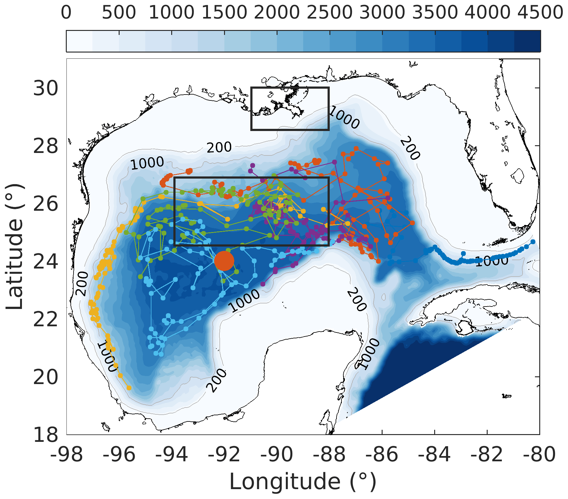
Figure 1Model bathymetry (unit: m) with trajectories of six bio-optical floats (small colored dots and lines) which were operated in the Gulf of Mexico from 2011 to 2015. The location of the 1D model is denoted by the large orange dot. The north and south black boxes represent the Mississippi Delta and the central gulf, respectively, to show comparisons of surface chlorophyll in Fig. S5.
The Gulf of Mexico (GOM) is a semienclosed marginal sea (Fig. 1) which is characterized by eutrophic coastal waters on the northern shelf and an oligotrophic deep ocean. The high productivity in the northern coastal region is fueled by large nutrient and freshwater inputs from the Mississippi and Atchafalaya rivers. The large nutrient load and strong stratification driven by Mississippi and Atchafalaya River inputs lead to summer hypoxia and ocean acidification in bottom waters on the northern shelf (Laurent et al., 2017; Yu et al., 2015), but nutrient export across the shelf break into the open gulf is minor (Xue et al., 2013).
The deep ocean of the GOM is oligotrophic. Previous satellite-based studies have revealed a clear seasonal cycle in surface chlorophyll, with the highest concentrations in winter and the lowest in summer (Martínez-López and Zavala-Hidalgo, 2009; Muller-Karger et al., 1991, 2015). Thanks to advances in autonomous profiling technology, recent studies based on simultaneous measurements of subsurface chlorophyll and backscatter have demonstrated that the seasonal variability of surface chlorophyll might be a result of the vertical redistribution of subsurface chlorophyll and/or physiological response to solar radiation of phytoplankton (Pasqueron de Fommervault et al., 2017; Green et al., 2014).
3.1 Biological observations
Monthly averaged satellite chlorophyll from the Ocean Colour Climate Change Initiative project (OC-CCI, http://www.oceancolour.com/, last access: 25 April 2017) with a spatial resolution of 4 km from 2010 to 2015 was used for model validation and parameter optimization. These data were provided by the European Space Agency (ESA), which produced a set of validated and error-characterized global ocean color products by merging SeaWiFS (Sea-viewing Wide Field-of-view Sensor), MODIS (Moderate Resolution Imaging Spectroradiometer), MERIS (Medium Resolution Imaging Spectrometer), and VIIRS (Visible Infrared Imaging Radiometer Suite) products.
In addition to the satellite-based measurements, bio-optical measurements from six autonomous profiling floats were used (Fig. 1), which were deployed by the Bureau of Ocean Energy Management (BOEM) and operated in the deep GOM from 2011 to 2015. These floats were equipped with a CTD and bio-optical sensors to collect biweekly profiles of temperature, salinity, chlorophyll, and backscatter at 700 nm (bbp700 (m−1)) from the surface to 1000 m depth (see Pasqueron de Fommervault et al., 2017; Green et al., 2014, for more details). Chlorophyll was derived from fluorescence based on the sensor manufacturer's calibrations and compared with the satellite estimates of surface chlorophyll. While the surface chlorophyll measurements from the floats and the satellite estimates both showed a typical seasonal cycle and were highly correlated (R2=0.74; see Figs. S1 and S2a in the Supplement), the satellite underestimated the float-measured chlorophyll concentrations in winter (Fig. S1c). Satellite estimates were therefore corrected following the regression equation shown in Fig. S2a.
Table 1Initial values and ranges of biogeochemical model parameters.
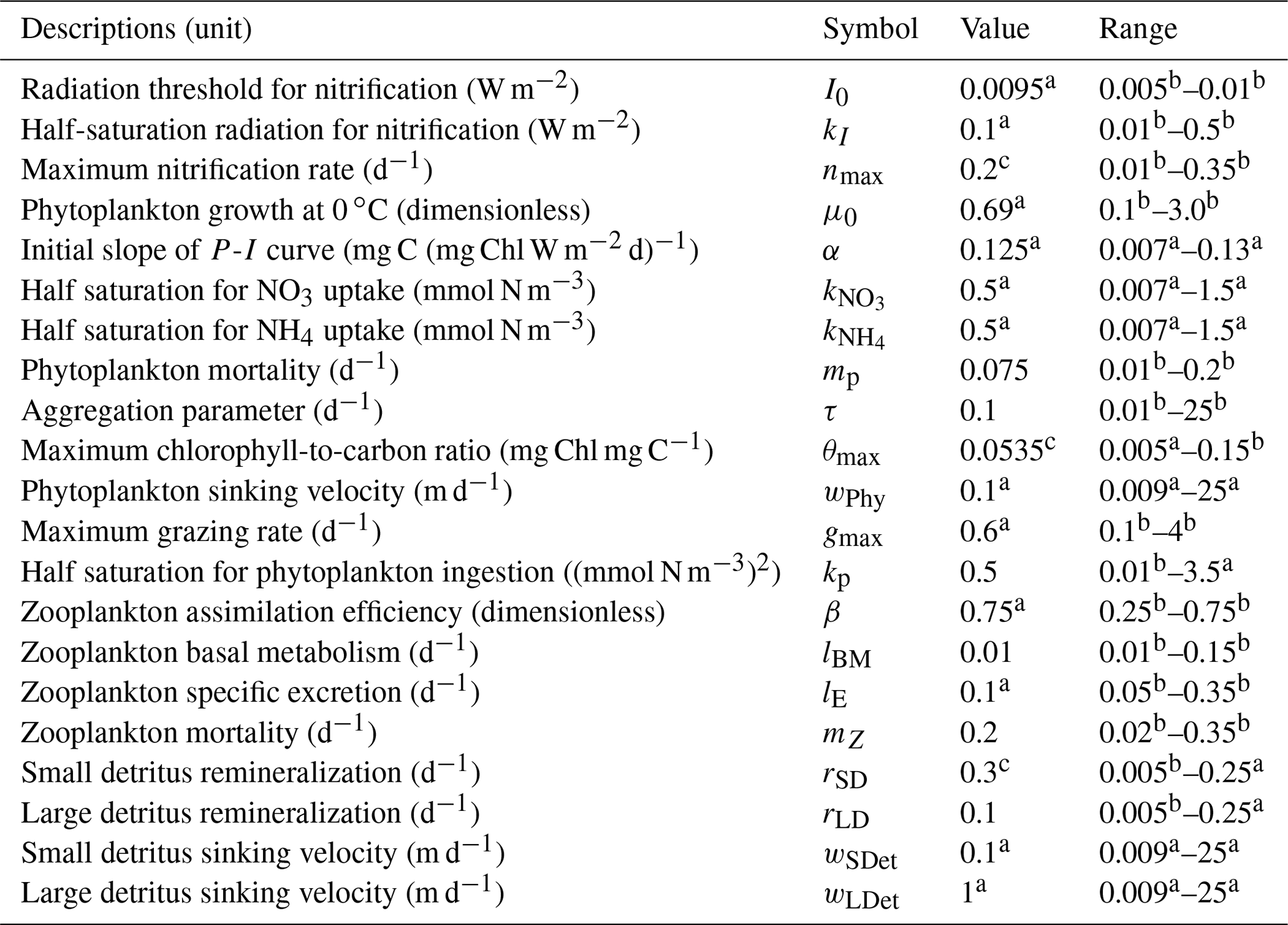
a Fennel et al. (2006). b Kuhn et al. (2018). c Yu et al. (2015).
The backscatter sensor carried by the floats provided the volume scattering function at a centroid angle of 140∘ and a wavelength of 700 nm (β(140∘, 700 nm) m−1 sr−1). The profiles were filtered (Briggs et al., 2011) to remove spikes and then converted into bbp700 following Green et al. (2014). After that, profiles of bbp700 were converted into bbp470 based on a power law (Boss and Haëntjens, 2016) to obtain the phytoplankton (mmol N m−3) and POC (mg C m−3) estimates:
where λ1 and λ2 represented the measured wavelength, and γ was estimated as 0.78 based on the global measurements. The relationships for phytoplankton (Martinez-Vicente et al., 2013, Eq. 2) and POC (Rasse et al., 2017, Eq. 3) were obtained from a dataset for the Atlantic Ocean that covered a wide range of oceanographic regimes from eutrophic to oligotrophic ecosystems. The scale factors of 12 and 6.625 in Eq. (2) represented the molecular weight of carbon and the Redfield ratio to convert phytoplankton concentrations from mg C m−3 to mmol N m−3. The intercept in Eq. (2) represented the background backscatter of nonalgal detritus, which based on Behrenfeld et al. (2005) was the backscatter value when chlorophyll was zero. However, in this study, the majority (87 %) of bbp470 in the upper 200 m was below the intercept, and the resulting phytoplankton concentrations were therefore close to zero, which is unrealistic in the Gulf of Mexico. Therefore, the satellite estimate of bbp670 from OC-CCI was converted into bbp700 and compared with the float measurements. Compared to surface chlorophyll, surface bbp700 has a less distinct seasonal cycle (Fig. S3). For example, the coefficient of variation, defined as the ratio between standard deviation and mean to show the extent of variability, is much lower for bbp700 (0.09 and 0.07 for floats and satellite, respectively) than for chlorophyll (0.31 and 0.26 for floats and satellite, respectively). The float bbp700 is weakly correlated with the satellite estimates (R2=0.11) and generally lower by a factor of ∼0.45 than the satellite estimates (Fig. S2b). The bbp700 profiles were therefore multiplied by 2.2 before being converted to bbp470. As a result, the mean value of the bbp470 ( m−1) is close to the intercept in Eq. (2) when chlorophyll went to zero. Furthermore, the resulting concentrations of phytoplankton biomass and POC as well as the ratio of chlorophyll to phytoplankton biomass are reasonable (please see Figs. 4 and 10). This gave us confidence in our conversion process for float backscatter and our choice of empirical equations relating backscatter to phytoplankton and POC.
3.2 Three-dimensional model description
The physical model was configured based on the Regional Ocean Modeling System (Haidvogel et al., 2008, ROMS, https://www.myroms.org, last access: 16 June 2016) for the Gulf of Mexico (Fig. 1). The model has a horizontal resolution of ∼5 km and 36 terrain-following sigma layers with refined resolution near the surface and bottom as in Yu et al. (2019). The model solved the horizontal and vertical advection of tracers using the multidimensional positive definitive advection transport algorithm (MPDATA, Smolarkiewicz and Margolin, 1998). Horizontal viscosity and diffusivity were parameterized by a Smagorinsky-type formula (Smagorinsky, 1963), and vertical turbulent mixing was calculated by the Mellor–Yamada 2.5-level closure scheme (Mellor and Yamada, 1982). Bottom friction was specified by a logarithmic drag formulation with a bottom roughness of 0.02 m. The model was forced by 3-hourly surface heat and freshwater fluxes; 6-hourly air temperature, sea level pressure, and relative humidity; and 10 m winds from the European Centre for Medium-Range Weather Forecast ERA-Interim product with a horizontal resolution of 0.125∘ (ECMWF reanalysis, https://www.ecmwf.int/en/forecasts/datasets/reanalysis-datasets/era-interim, last access: 17 August 2018). A bulk parameterization was applied to calculate the surface net heat fluxes and wind stress. The model was one-way nested inside the 1∕12∘ data-assimilative global HYCOM/NCODA (https://www.hycom.org, last access: 2 November 2017). Tidal constitutes were neglected in the model.
The biogeochemical model used a seven-component model (Fennel et al., 2006) to simulate the nitrogen cycle in the water column. The model described the dynamics of two species of dissolved inorganic nitrogen (nitrate, NO3, and ammonium, NH4), one function of phytoplankton (Phy), chlorophyll (Chl) as a separate state variable which allowed photo-acclimation based on the model of Geider et al. (1997), one function of zooplankton (Zoo), and two pools of detritus (i.e., small suspended detritus, SDeN, and large fast-sinking detritus, LDeN). Water–sediment interactions were simplified by an instantaneous remineralization parameterization, where detritus sinking out of the water column immediately resulted in a corresponding influx of ammonium into the bottom layer. Detailed descriptions of the model equations can be found in Fennel et al. (2006) and Laurent et al. (2017). The biological model parameters are listed in Table 1.
The model received freshwater, nutrients (NO3 and NH4), and organic matter inputs from major rivers along the Gulf Coast. Freshwater and nutrients from the Mississippi and Atchafalaya rivers were prescribed based on the daily measurements by the US Geological Survey river gauges. River particulate organic nitrogen (PON) was assigned to the small detritus pool and determined as the difference between total Kjeldahl nitrogen and ammonium (Fennel et al., 2011). Other rivers utilized the climatological estimates of freshwater, nutrients, and PON as in Xue et al. (2013).
Initial and open boundary conditions for NO3 were specified by applying an empirical relationship between NO3 and temperature, derived from the World Ocean Atlas (WOA; Fig. S4a), that was applied to the temperature fields from HYCOM/NCODA. Analogously, empirical relationships between chlorophyll and density (Fig. S4b), phytoplankton and density (Fig. S4c), and POC and density (Fig. S4d) were obtained from the median profiles of the bio-optical floats and used to derive initial and boundary conditions for these variables. Zooplankton and small detritus were assumed to amount to 10 % of phytoplankton biomass and the remaining fractions of POC attributed to large detritus. Sensitivity tests showed that changing these allocations had little impact on our model results.
A 6-year (5 January 2010–31 December 2015) hindcast was performed that included the period of operation of the bio-optical floats. The first year was considered model spin-up and the next 5 years are discussed.
3.3 One-dimensional model description
As optimizing a 3D biogeochemical model is computationally expensive, it was more practical to perform the optimization using a reduced-order model surrogate. A surrogate can be a coarser-resolution model, a simplified model, or a reduced-dimension model. In this study, a 1D model was used to optimize the biological parameters of the 3D model. This approach has been successfully used previously (Hoshiba et al., 2018; Kane et al., 2011; Oschlies and Schartau, 2005).
The 1D model, which is similar to that used by Lagman et al. (2014) and Kuhn et al. (2015), covered the upper 200 m of the ocean with a vertical resolution of 5 m and was configured at one location in the open gulf (see Fig. 1). This relatively fine vertical resolution was used because it was close to that of our BGC-Argo floats (4–6 m in upper 200 m) and was much higher than the 3D model whose vertical resolution varies from a few meters near the surface to about 50 m near at 200 m depth around the 1D station. In the vertical direction, the water column was divided into two layers: the turbulent surface layer and a quiescent layer below. A higher diffusion coefficient (), in unit of m2 d−1) was applied in the turbulent surface layer, and a lower diffusion coefficient () was assigned to the quiescent bottom layer. The interface between these two layers was determined by the mixed layer depth (HMLD, in unit of m), defined as the depth where the temperature was 5 ∘C lower than at the surface, and was obtained from daily outputs of the 3D model. The model was integrated in time using the Crank–Nicolson scheme for vertical turbulent mixing and an implicit time-stepping scheme for the biogeochemical tracers, which were treated identically to the 3D model. Some of the biogeochemical parameterizations required input of temperature and solar radiation, which were also taken from the 3D model. As the 1D model did not consider horizontal and vertical advection, NO3 below 100 m was nudged to that from the 3D base simulation with a nudging timescale of 20 d. The 1D model was run for the year 2010 repeatedly for three cycles, with the first two being model spin-up and the last annual cycle used to calculate the misfit between the model and observations.
3.4 Parameter optimization method
The evolutionary algorithm described by Kuhn et al. (2015, 2018) was used to search for optimal model parameters by minimizing the misfit between the model and observations. The misfit was measured by the following cost function:
where represented the parameters vector, V was the number of different observation types, Nv was the number of observations for each variable, and was the misfit for observation type v measured as the mean-square difference between observations () and corresponding model estimates (). The cost function was normalized by the standard deviation of each variable type (σv) in order to remove the effect of different units.
The algorithm is inspired by the rules of natural selection. Following Kuhn et al. (2015), an initial parameter population of 30 parameter vectors was randomly generated within a predefined range of parameters (see Table 1). The model was evaluated for each parameter vector and the resulting cost function was calculated. For this initial generation and each of the following generations, the half of the population with the lower misfit survived into the next generation. The other half was regenerated through a recombination of survivors in a process analogous to genetic crossover. In addition, each newly generated population was subject to random mutations by multiplying the parameter values by a random value between 0 and 2. Parameter values exceeding the predefined range were replaced by their corresponding minimum or maximum limits to avoid unrealistic values. The above procedure was performed iteratively for 300 generations to reach the minimum of the cost function, which corresponded to the optimal parameter set.
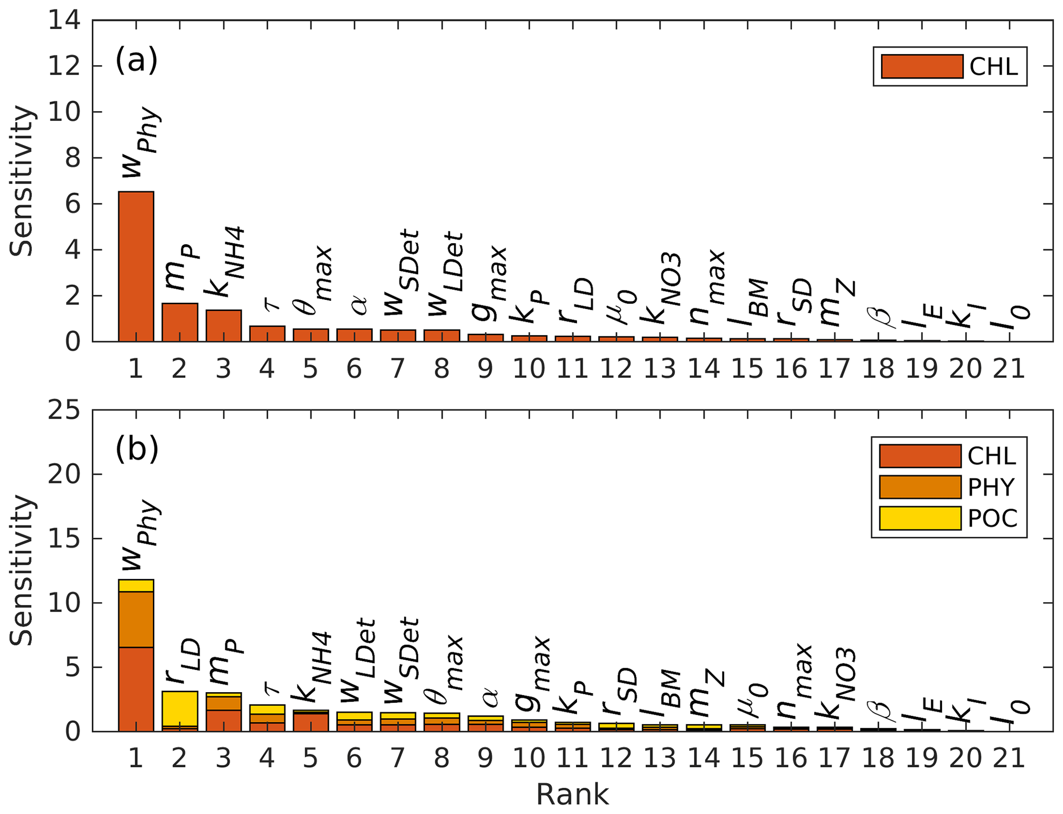
Figure 2Parameter sensitivities (unit: dimensionless) with respect to (a) chlorophyll and (b) the sum of chlorophyll, phytoplankton, and POC.
Previous parameter optimization studies have shown that it is difficult to constrain all model parameters even for very simple ecosystem models because the information content of available observations is typically insufficient (Matear, 1995; Fennel et al., 2001; Ward et al., 2010). Here we conducted sensitivity tests to identify the parameters that were most sensitive to the available observations and chose a subset of these to be optimized. In the base case, all parameters were at their initial guess values obtained from the previous literature and some initial tuning (Table 1). Then the test cases were run multiple times by incrementally changing one parameter at a time to be the minimum; the first, second, and third quartile; and the maximum of its corresponding range while setting the other parameters to their initial guess value (Table 1). The sensitivity was measured as the sum of a normalized absolute difference between the base case (yBase) and the test case (yTest):
where m is the number of parameter increments (here 5) and n is the number of base–test pairs consisting of all 1D model grid cells throughout the whole simulation period for all variables to be compared.
Results of the sensitivity analysis are shown in Fig. 2, where parameters are ranked by sensitivity with respect to chlorophyll (Fig. 2a) and the sum of chlorophyll, phytoplankton, and POC (Fig. 2b). POC is the sum of phytoplankton, zooplankton, and small and large detritus.
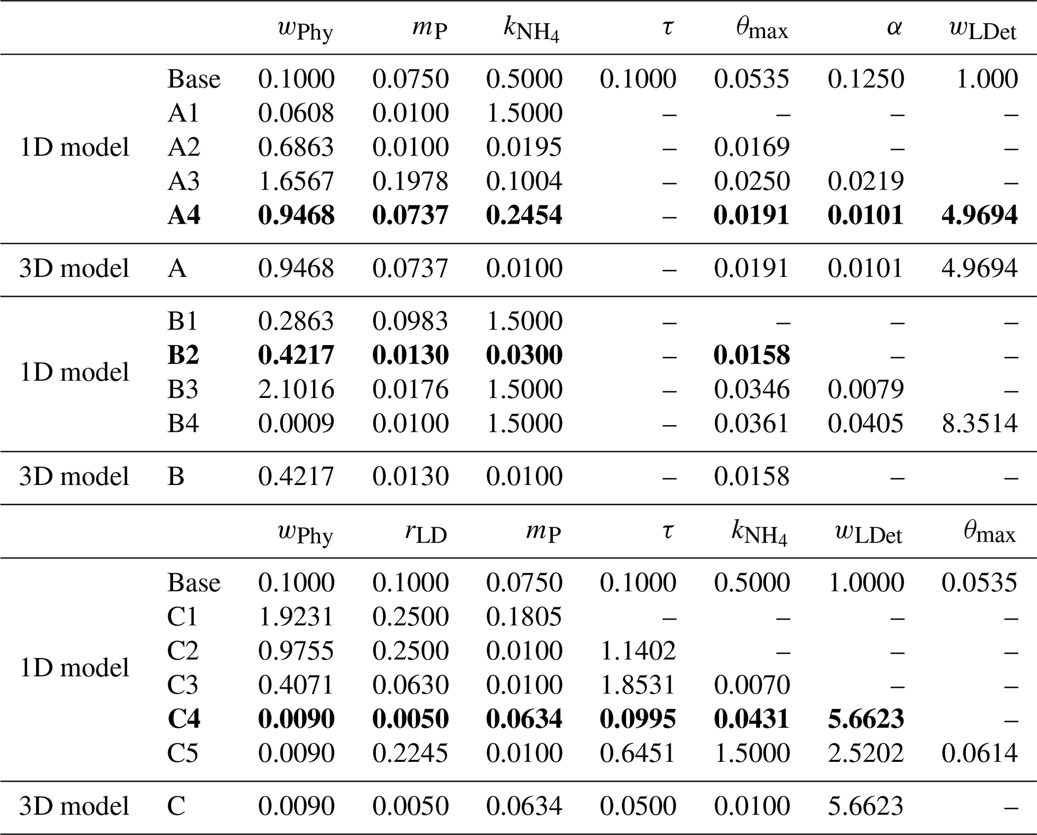
Table 2The best fit of parameter set for each optimization experiment. Dashed lines represent that these parameters are not included in the parameter optimization and use their prior values. The optimal optimization A4, B2, and C4 which are further discussed and are denoted simply as experiment A, B, and C are highlighted as bold.
3.5 Parameter optimization experiments
For the parameter optimization of the 1D model, satellite chlorophyll within a 3 pixel × 3 pixel (12 km × 12 km) area around the 1D station and monthly climatological profiles from the BGC-Argo floats were used. For the climatological profiles, all float profiles in the gulf were averaged because the deep Gulf of Mexico is homogenous horizontally and only few profiles were available in the immediate vicinity of the 1D station.
To assess the effects of the optimization with respect to the different observation types, we conducted three groups of experiments in which (A) surface satellite chlorophyll only, (B) surface satellite chlorophyll and float profiles of chlorophyll, and (C) surface satellite chlorophyll and float profiles of chlorophyll, phytoplankton, and POC were used. For each of these three groups, four to five optimizations were conducted, starting with the three most sensitive parameters and then adding one more parameter at a time (Table 2) guided by the sensitivity analysis with respect to the observed variables they used. Specifically, groups A and B were based on the sensitivity analysis with respect to chlorophyll, while group C was based on the sensitivity analysis with respect to the sum of chlorophyll, phytoplankton, and POC. Each optimization was replicated four times. The optimization with the smallest model–data misfit within each group was then used. Prior tests have shown that the available observations cannot simultaneously constrain the sinking rates of small and large detritus (wSDet and wLDet) because an increase in one parameter can be counteracted by a decrease in the other. Therefore, a constant ratio of 0.1 between these two parameters () was imposed based on their prior values, and only one of the two was optimized. In groups A and B, the aggregation parameter τ was fixed at 0.05 because prior tests generated unreasonably high values for this parameter.
We report two different metrics of misfits for these groups of experiments. The first metric, which we refer to as the case-specific cost function value, is based on the optimized observations in a given experiment and was minimized by the optimization algorithm, i.e.,
However, the models with lower case-specific misfit do not necessarily have better predictive skill in reproducing the unoptimized observations because of the so-called overfitting problem; e.g., the model might be tuned to reproduce optimized observations through wrong mechanisms (Friedrichs et al., 2006). To account for this, a second metric referred to as the total misfit is given by Eq. (9). For group C, the second metric is the same as the case-specific cost function. For groups A and B, the total misfit metric allows us to assess improvements in the model’s predictive skill to represent unoptimized fields.

Figure 3Annual cycle of surface chlorophyll (a), vertically integrated chlorophyll (b), vertically integrated phytoplankton (c), vertically integrated POC (d), and the depth (e) and magnitude (a) of the DCM from observations (black dots with error bars); the base case (black lines); and experiment A (orange lines; only satellite surface chlorophyll is used), B (yellow lines; satellite surface chlorophyll and float profiles of chlorophyll are used), and C (blue lines; all available observations are used). Chlorophyll, phytoplankton, and POC are integrated over the top 200 m. Black error bars represent the interquartile range of observations.
4.1 Observations and base case
To provide context for the evaluation of our optimization experiments, the observations and the base case will be described first. As shown in Fig. 3a, the observed surface chlorophyll shows a clear seasonality with the high concentrations in winter and low concentrations in summer. In the base case, the simulated surface chlorophyll fits observations well. Unlike the surface chlorophyll, the observed integrated chlorophyll as well as the phytoplankton and POC over the upper 200 m tend to be more constant with much less seasonality (Fig. 3b–d). This has been reported by Pasqueron de Fommervault et al. (2017), who attributed the seasonality of surface chlorophyll to the vertical redistributions of subsurface chlorophyll and/or photoacclimation rather than real changes in biomass.
The DCM is a ubiquitous phenomenon in the oligotrophic regions and can form independently of the biomass maximum (Cullen, 2015; Fennel and Boss, 2003). In this study, we define the DCM depth as where the maximum of subsurface chlorophyll is. Observations detect a predominant DCM at around 60–100 m depth throughout the whole year, with a sharp deepening in June and gradual shoaling after July (Fig. 3e), reflecting the seasonality of the solar radiation. Unlike the large variability in the depth of the DCM, its magnitude is relatively constant at around 0.62 mg m−3 (Fig. 3f). In the annually averaged profiles, the observed DCM is located at about 80 m depth with a concentration of 0.52 mg m−3 (Fig. 4a). The base case succeeds in reproducing the DCM at 65±7 m depth. However, it fails to reproduce the deepening of the DCM in June, and the simulated annually averaged depth of DCM is shallower by about 15 m than the observed. The simulated magnitude of the DCM is about 2-fold larger than the observed (Figs. 3f and 4a), and hence the base case generally overestimates vertically integrated chlorophyll (Fig. 3b).
With respect to phytoplankton and POC, the observed maximum concentration occurs at about 60 m depth, which is 20 m above the DCM (Fig. 4b–c). The observed vertical distributions of phytoplankton and POC are not well captured by the base case. For example, phytoplankton and POC in the upper layer are overestimated with the model–data discrepancies exceeding the variability of the observations (Fig. 4b–c). As a result, the base case yields an overall overestimation of the vertically integrated phytoplankton and POC (Fig. 3c–d).
Figure 4b also shows that both observed and simulated phytoplankton approach zero at about 160 m depth. Unlike phytoplankton, the observations show that the POC concentrations are 19 mg C m−3 at about 200 m depth because of the existence of detritus, or zooplankton, or both (Fig. 4b, c). However, the base case fails to reproduce these nonzero POC concentrations, indicating that the model might be underestimating the carbon export fluxes at 200 m.
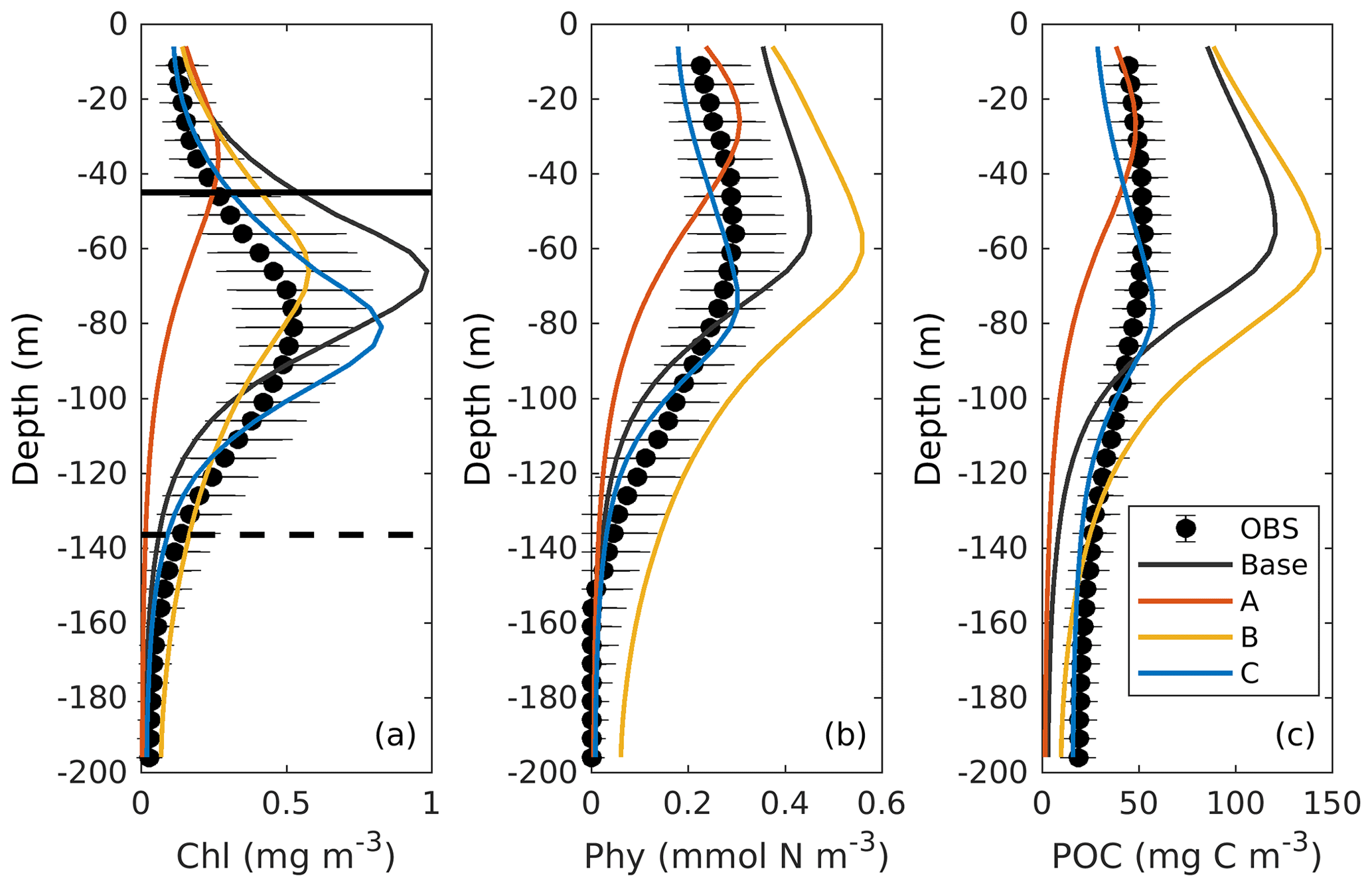
Figure 4Observed (black dots with error bars) and simulated (colored lines) vertical profiles of chlorophyll, phytoplankton, and POC. Black errors represent the interquartile range of observations. The solid and dashed black lines in (a) represent the median values of mixed layer depth from July and December.
4.2 Results of the optimizations
4.2.1 Model–data misfits
The case-specific cost function values and total misfits for the different 1D optimizations are shown in Fig. 5. Not surprisingly, all optimizations result in a reduction of the case-specific cost function values. The extent of the reductions depends on the specific subset of parameters that were optimized. However, the total misfits are not reduced in all optimizations. Optimizations A1 and A2 lead to slightly larger total misfits than the base case, and optimization B2 leads to a significantly larger total misfit. The smallest total cost function values are achieved in A4, B4, and C4, i.e., in the experiments where a larger subset of parameters was optimized (six parameters). The optimal parameter sets (A4, B2, and C4), which are selected based on case-specific misfit from these three groups, will be used in subsequent analyses and hereafter are denoted simply as experiment A, experiment B, and experiment C. Further comparisons are presented below to assess the impact of the different combinations of observations.
4.2.2 Experiment A: satellite chlorophyll only
The optimal parameters (Table 2) from experiment A yield a 58 % reduction in the misfit for surface chlorophyll (Fig. 5d). However, the vertical structure of chlorophyll deteriorates relative to the base case (Fig. 4a) because of inappropriate estimates of the initial slope (α=0.0101; see Table 2) and the maximum ratio of chlorophyll to carbon (θmax=0.0191; see Table 2). The annually averaged depth of the DCM is lifted up to around 30±10 m, and the magnitude of DCM strongly decreases (Figs. 3a, 4b). Similar to chlorophyll, these deteriorations also manifest in the vertical phytoplankton and POC distributions (Fig. 4b–c). As a result, experiment A underestimates vertically integrated chlorophyll, phytoplankton, and POC (Fig. 3b–d).
4.2.3 Experiment B: satellite chlorophyll and chlorophyll profiles
Due to the addition of observed chlorophyll profiles to the optimization in experiment B, the misfits for surface and subsurface chlorophyll decrease relative to the base case (Fig. 5d), but the reduction in the misfit for surface chlorophyll (38 %) is smaller than that in experiment A (58 %). A straightforward interpretation is that the addition of subsurface observations reduces the model's degrees of freedom to fit one single observation type (surface chlorophyll). The vertical profile of chlorophyll is reproduced better in experiment B than in the base case and experiment A in that the magnitude of the DCM is closer to the observations, although the DCM depth is still too shallow, on average by about 20 m (Fig. 4a). The improvement in the vertical chlorophyll structure results in a better model–data fit of vertically integrated chlorophyll (Fig. 3b).
Despite the improvements in chlorophyll, the vertical profiles of phytoplankton and POC exhibit a marked deterioration relative to the base case and experiment A (Fig. 4b–c) because the parameter optimization underestimates the maximum chlorophyll-to-carbon ratio (θmax=0.0158; see Table 2). Experiment B leads to an overestimation of phytoplankton and POC relative to the base case with misfits roughly 2.7 and 1.6 times larger than those of the base case, respectively (Fig. 5d). Although experiment B reproduces the non-zero POC concentrations at about 200 m depth, the proportion of phytoplankton in the POC pool is incorrect. In contrast to the observations where the phytoplankton's contribution is negligible (Fig. 4), the simulated POC at 200 m is dominated by phytoplankton (49 %).
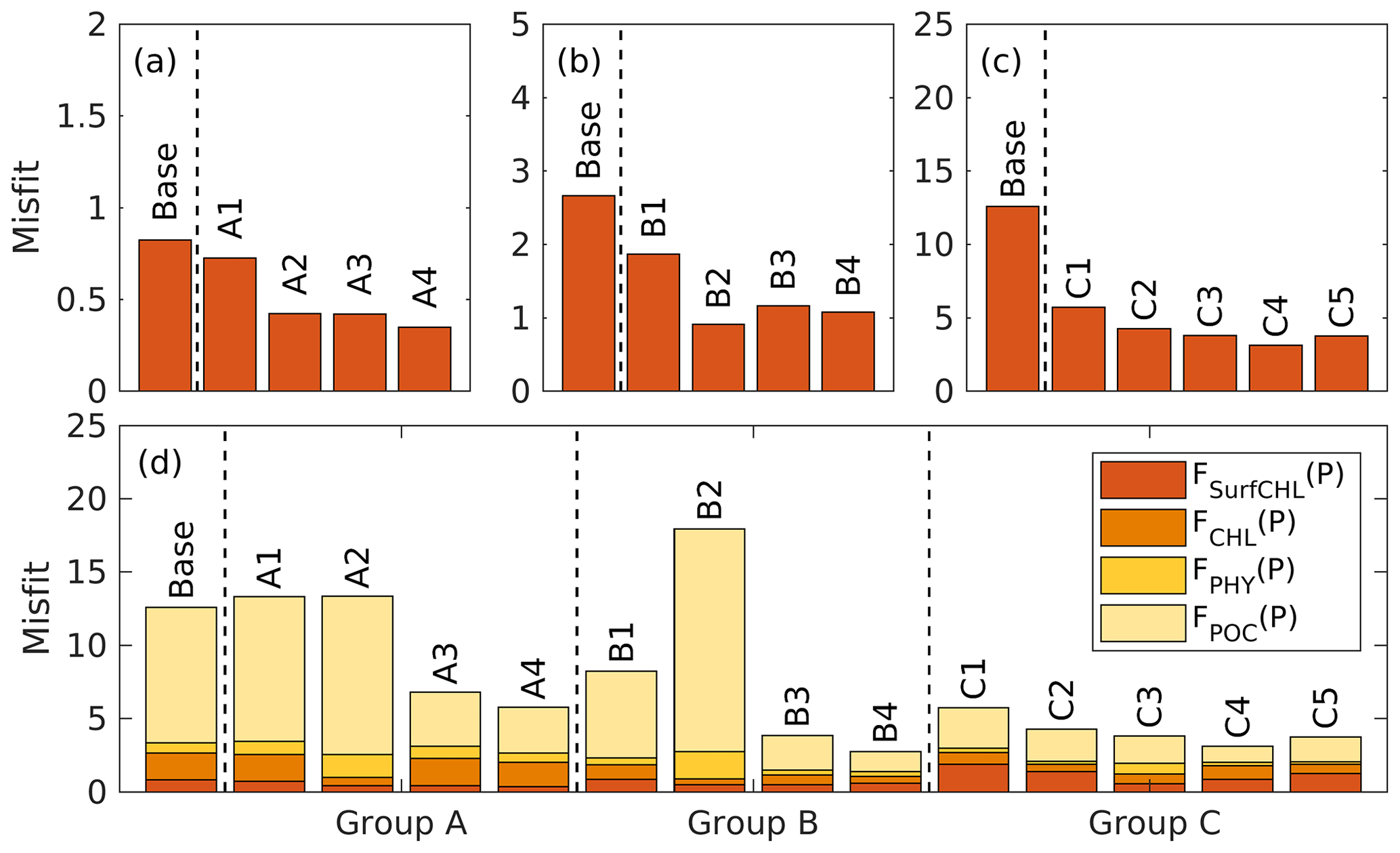
Figure 5The case-specific cost function values (a–c) and total misfits (d) of the base case and the different optimizations.
4.2.4 Experiment C: all available observations
Incorporating all observations (i.e., surface chlorophyll and profiles of chlorophyll, phytoplankton, and POC) in experiment C improves the model–data misfits for almost all aspects except for surface chlorophyll (Fig. 3). Although a slight increase in the misfit occurs for the surface chlorophyll (∼5 %), the total misfit is reduced by 75 % compared to the base case. As shown in Fig. 4a, the annually averaged depth of DCM of 80 m coincides with the observed DCM, primarily because experiment C reproduces the deepening of the DCM in summer. The magnitude of the DCM is also decreased relative to the base case but remains higher than the observed. Phytoplankton and POC profiles exhibit only minor deviations from the observations (Fig. 4b–c). Importantly, experiment C reproduces the non-zero POC concentrations at 200 m. In contrast to experiment B, phytoplankton in experiment C drops to zero at about 160 m and POC is dominated by detritus (85 %), which is more consistent with the observations.
4.3 Simulated carbon fluxes
Annually averaged carbon fluxes within the upper 200 m are shown for each experiment in Fig. 6. The primary production in the base case amounts to 0.78 g C m−2 d−1, of which 37 % is consumed by zooplankton, and the remaining 63 % flows into detritus pools through sloppy feeding, mortality, and aggregation of phytoplankton. As for the production of detritus, contributions from the phytoplankton and zooplankton pools account for 70 % and 30 %, respectively. Most of the produced detritus is recycled into the nutrient pool fueling recycled primary production, and only a small fraction is removed from the upper layer through gravitational sinking. As a result, carbon export, which is estimated as the sum of sinking fluxes by phytoplankton and detritus, is only 0.00032 g C m−2 d−1 and accounts for 0.04 % of primary production.
Due to the underestimation of phytoplankton in experiment A, primary production is reduced to 0.21 g C m−2 d−1 in that case. All other fluxes in the top 200 m decrease relative to the base case as well, except for the export flux which increases to about 0.8 % of primary production. This relative increase in export is the result of larger sinking rates of phytoplankton and detritus (wPhy=0.95, wLDet=4.97; see Table 2) than those used in the base case.
In contrast to experiment A, experiment B yields an increase in primary production relative to the base case. The proportion of the grazing flux to primary production and the contribution of zooplankton to the production of detritus also increase to about 59 % and 52 %, respectively. Unlike in the other three experiments, carbon export in experiment B is dominated by the sinking of phytoplankton, reflecting its large contribution to POC at 200 m. Although the simulated POC concentration at 200 m is very close to the observations, the relative contributions of phytoplankton, zooplankton, and detritus are problematic and likely do not result in a better estimation of carbon export (in this case 0.3 % of primary production).
In experiment C, primary production is 0.30 g C m−2 d−1, with 24% flowing to zooplankton. The mortality of zooplankton causes a flux of 0.047 g C m−2 d−1 to detritus, which accounts for 17 % of the production of detritus. Finally, about 24 % of primary production is removed from the upper 200 m through gravitational sinking. The simulated export ratio of 24 % is within the wide range of reported export ratios, from 6 % to 43 %, at 120 m depth in the Gulf of Mexico (see Table 3 of Hung et al., 2010). Despite the high degree of uncertainty that exists when estimating export ratios (e.g., the global mean export ratio varies from ∼10 % Henson et al., 2012; Lima et al., 2014; Siegel et al., 2014 to ∼20 % Henson et al., 2015; Laws et al., 2000), it is obvious that only experiment C reproduced an export ratio of a reasonable magnitude. A more detailed validation of primary production and export fluxes will be presented in the following sections.
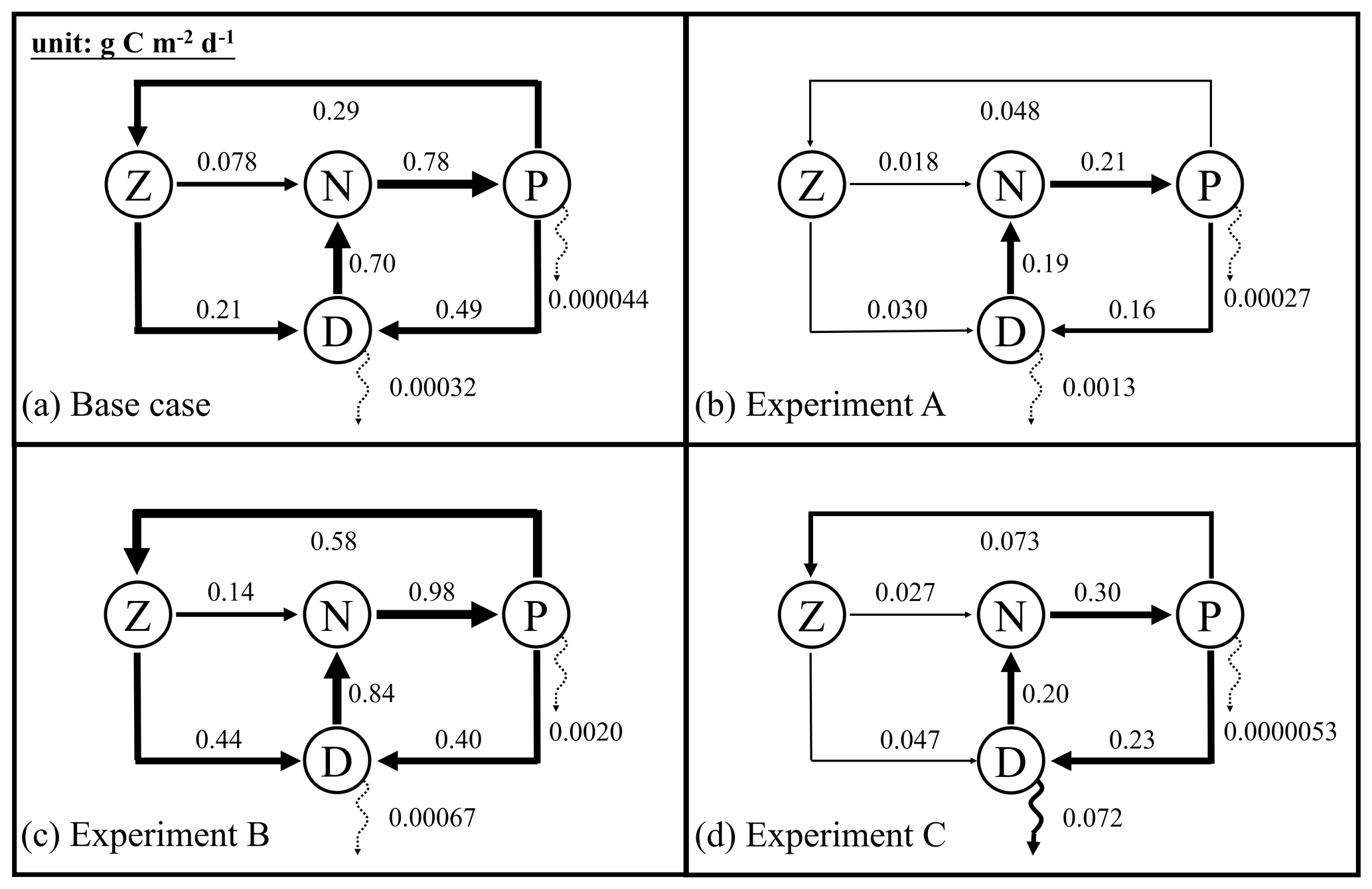
Figure 6Annually averaged carbon fluxes integrated over the upper 200 m (unit: g C m−2 d−1) for the base case (a) and optimized experiments A, B, and C. The N, P, Z, and D stand for the pools of nutrient, phytoplankton, zooplankton, and the sum of small and large detritus, respectively. The thickness of arrows scales with the magnitude of fluxes. Dashed arrows represent fluxes lower than 0.01 g C m−2 d−1.
The optimal parameter sets from the 1D optimizations of A, B, and C were applied in the 3D model for the whole GOM for 5 years (2011–2015). The performance of the 3D model can be regarded as a cross validation of the parameters optimized in 1D at different times and locations. It is possible that the optimization algorithm has modified parameters to compensate for biases between 1D and 3D simulations, e.g., the absence of advection in 1D model as well as the differences in the model domain, model period, and model resolution, that degrade the 3D model performance (Kane et al., 2011). Indeed, directly applying the optimal parameter sets from the 1D version to the 3D model yields lower model–data agreement than the 1D counterpart but preserves the most important features well. For instance, when the resulting parameters were used in experiment C, chlorophyll concentrations in the upper layer were lower in the 3D model and farther away from the observations. However, the DCM depth and the non-zero POC concentrations at 200 m with appropriate contributions from each component are well reproduced in the 3D model. We therefore performed a few manual tests and made the following modifications to the optimized parameters to bring the model–data agreement of the 3D model in better alignment with that of the 1D version (Table 2): the half saturation for NH4 uptake () was decreased to 0.01 in experiment B and C, and the aggregation parameter (τ) was decreased to 0.05 in experiment C.
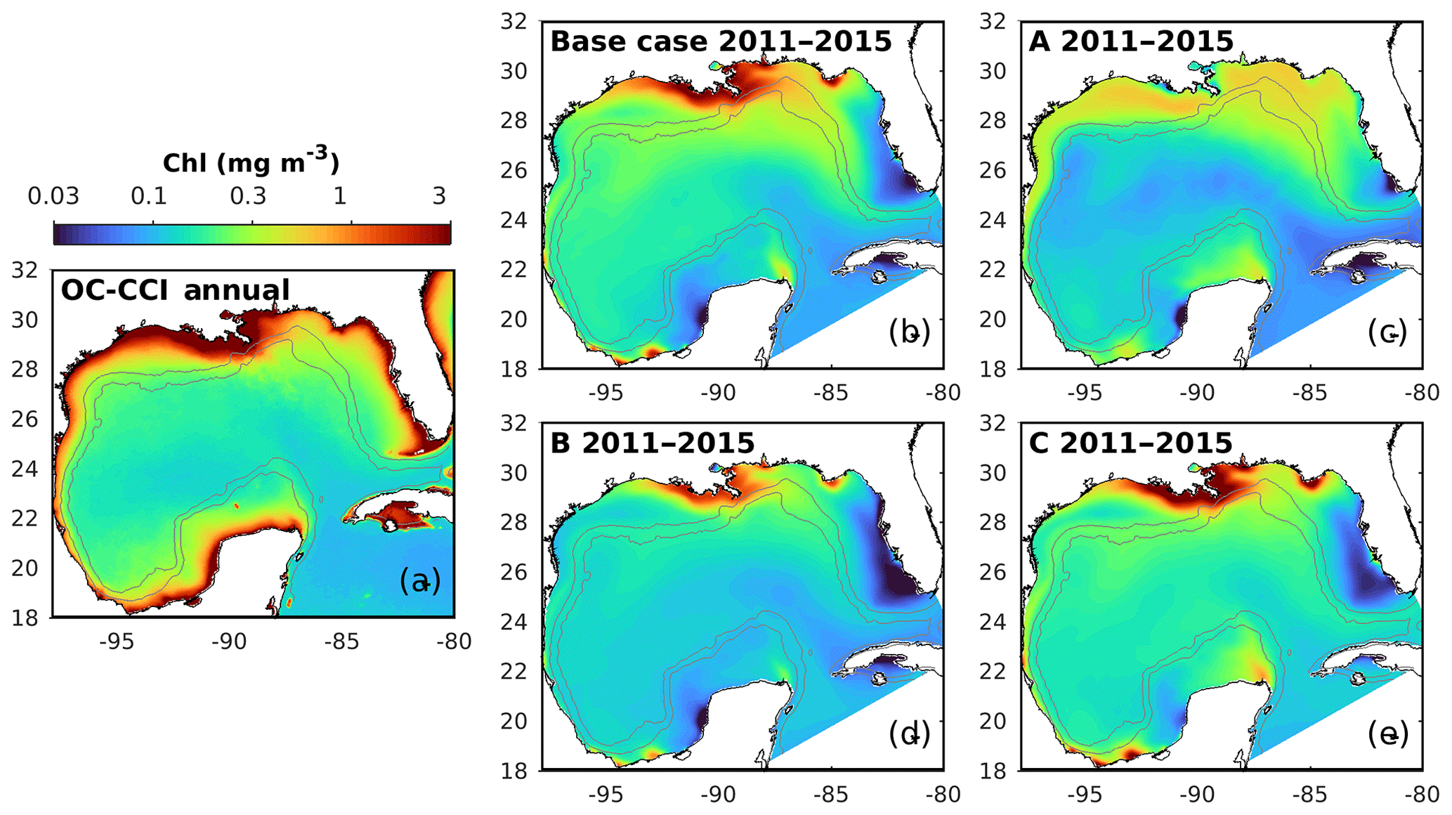
Figure 7Spatial distributions of the annual mean chlorophyll in the surface layer from the satellite (OC-CCI) climatology (2011–2015) and the different model versions. The gray contours mark the bathymetric depths of 200 and 1000 m.
5.1 Spatial patterns of surface chlorophyll
First, the annual climatological surface chlorophyll from the satellite and model are compared from 2011 to 2015. The satellite estimates show high chlorophyll in the coastal regions and low chlorophyll in the deep ocean (Fig. 7a). This spatial pattern of surface chlorophyll is well reproduced in all simulations except in experiment A, which even fails to reproduce the relatively high chlorophyll near the Mississippi–Atchafalaya River systems because of the high sinking rate of phytoplankton (wPhy=0.95; see Table 2). The largest model–data differences occur in the coastal regions, where all simulations underestimate the observed surface chlorophyll. Since all BGC-Argo floats operated in the deep ocean (Fig. 1) and the parameter optimization is performed at one central station without any influence from coastal environments, only the model results in the deep ocean (depth >1000 m) will be considered in the following discussion.
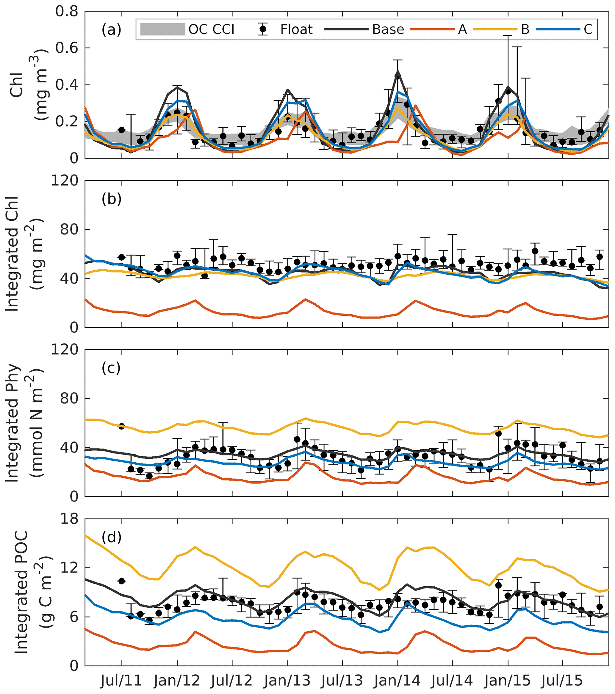
Figure 8Observed and simulated seasonal cycles of surface chlorophyll (a), vertically integrated chlorophyll (b), vertically integrated phytoplankton (c), and vertically integrated POC (d) from each 3D model. Solid lines represent the median values over the deep ocean of GOM (depth >1000 m). Error bars and shades show the 25 % and 75 % percentiles. Chlorophyll, phytoplankton, and POC are integrated over the top 200m.
5.2 Subsurface distributions
Figure 8 shows the seasonal cycles of surface chlorophyll as well as the vertically integrated chlorophyll, phytoplankton, and POC within the deep ocean (depth >1000 m). Analogous to the 1D models, chlorophyll, phytoplankton, and POC were integrated over the upper 200 m. Here again the whole deep ocean was averaged because it is homogenous horizontally. In addition, we compare surface chlorophyll with satellite estimates in two subregions from the Mississippi Delta and the central gulf in Fig. S5.
Comparisons of vertical profiles between observations and model results are given in Fig. 9. In general, the main features in the 3D models are very similar to those in 1D. Experiment A cannot constrain the vertical profiles of chlorophyll because of the inappropriate estimation of initial slope (α), experiment B overestimates phytoplankton and its contribution to POC since the maximum ratio of chlorophyll to carbon (θmax) is weakly constrained, and experiment C shows significant improvements in the model–data agreement.
Additional comparisons of the chlorophyll-to-carbon ratio, primary production, and carbon export fluxes from 1D and 3D models with observations are given in Fig. 10. The chlorophyll-to-carbon ratio is estimated as the vertically integrated chlorophyll divided by phytoplankton in the upper 200 m (Fig. 10a). As an important indicator of phytoplankton physiological status (Geider, 1987), the observed chlorophyll-to-carbon ratio varies considerably in response to the ambient environment. In general, the ratios derived from the 3D models are lower than their corresponding 1D values, but the differences are still within the range of variability. Without utilizing the observations of phytoplankton and POC, experiments A and B in both the 1D and the 3D versions underestimate the chlorophyll-to-carbon ratio. In experiment C, the simulated chlorophyll-to-carbon ratios from 1D and 3D are in good agreement with the observations although the observed variability is underestimated.
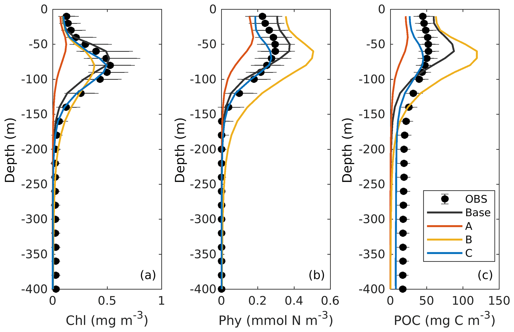
Figure 9Observed and simulated vertical profiles of chlorophyll, phytoplankton, and POC from each 3D model.
For reference, satellite-based primary production (PP) is provided by two algorithms, the Vertically Generalized Production Model (VGPM, Behrenfeld and Falkowski, 1997) and the Carbon-based Productivity Model (CbPM, Westberry et al., 2008). As shown in Fig. 10b, satellite-based PP differs depending on the algorithm applied. PP results from all 3D simulations which were integrated down to 200 m are qualitatively similar to the 1D simulations. Experiment C provides the best estimates of PP when compared to satellite-based estimates from VGPM and CbPM, both in 1D and 3D.
The base case and experiments A and B yield carbon export fluxes smaller by 1 to 2 orders of magnitude than experiment C. Thus, only experiment C from the 1D and 3D models are shown in Fig. 10c in comparison to observations from sediment traps (see Supplement). The carbon export fluxes at 200 m from the 1D and 3D are similar in magnitude although the 1D model yields higher fluxes and larger variability. Despite the scarcity of carbon export observations in the GOM, the model estimates are within the range of observations down to ∼1600 m and capture the observed declining trend of carbon export with depth.
In summary, all the results above demonstrate the feasibilities of using the locally optimized parameters from the 1D model to improve the 3D simulation. In addition, by incorporating all available observations (i.e., surface chlorophyll from satellite estimates, profiles of chlorophyll, phytoplankton, and POC from bio-optical floats), experiment C cannot only simulate the biogeochemical processes well in the upper 200 m, but also reproduce the carbon export flux and its associated attenuation in the deep ocean (200–1600 m) of the GOM.
6.1 Trade-offs between different observations for parameter optimization
The results of the optimization experiments vary dramatically depending on how many observation types are used. Using only satellite surface chlorophyll in experiment A succeeds in reducing the misfits of surface chlorophyll, but at the expense of the vertical structure since the predominant DCM disappears in experiment A. Satellite surface chlorophyll alone cannot constrain several vital parameters, including the initial slope of the productivity–irradiance curve (α) and the maximum ratio of chlorophyll to carbon (θmax), with confidence. This result highlights the importance of subsurface observations for parameter optimization and similarly for model validation.
The floats provide valuable subsurface observations, but chlorophyll profiles alone are not sufficient for parameter optimization. In experiment B, the addition of chlorophyll profiles leads to significant improvements in vertical chlorophyll distributions; however, the profiles of phytoplankton and POC deteriorate largely because the maximum ratio of chlorophyll to carbon (θmax) is poorly constrained. Using estimates of phytoplankton biomass and POC derived from backscatter measurements in experiment C yields the best estimation of plankton-related state variables and carbon fluxes (i.e., primary production and carbon export). Only in this experiment do the improvements obtained from observations in the upper 200 m extend to the deep ocean as reflected in the improved carbon export estimates below 1000 m.
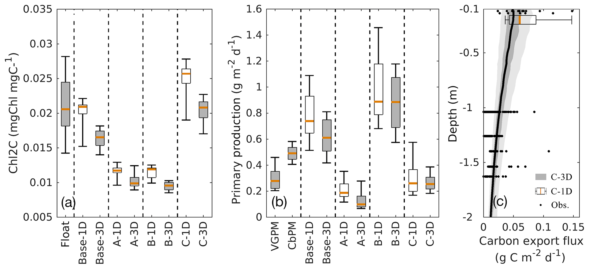
Figure 10Comparisons of the chlorophyll-to-carbon ratio (a), primary production (b), and carbon export fluxes (c) between the 1D and 3D models.
It should be noted, however, that degradation of unoptimized variables did not occur in all optimizations within experiments A and B. In some cases, the unoptimized fields were improved. For example, the A2 optimization yields a 69 % reduction in the misfit for subsurface chlorophyll (Fig. 5d) and large improvements of chlorophyll profiles (Fig. S6a) even though no observations of subsurface chlorophyll are used. Another example is that B1 optimization improves simulations of phytoplankton and POC (Figs. 5d and S6b–c) through the correlations between the observed chlorophyll and phytoplankton (R2=0.69) and POC (R2=0.69). Similar findings have been reported in Prunet et al. (1996a), where the improvements of chlorophyll profiles within the mixed layer were obtained by using surface chlorophyll in a 1D model. In a more recent study by Xiao and Friedrichs (2014a), where satellite data were used, subsurface fields were improved in addition to surface fields.
In optimizations A2 and B1, the improvement in unoptimized fields occurred because the poorly constrained parameters were not optimized but well defined coincidently (α=0.125 in the optimization A2 and θmax=0.0535 in the optimization B1; see Table 2). Including the poorly constrained parameters into the parameter optimization can return a lower misfit with respect to the observations used in optimization but increases the risk of overfitting and reduces the model's predictive skill, i.e., the ability to simulate unoptimized observations and those collected at different locations and times. This is consistent with previous studies (Friedrichs et al., 2006, 2007; Ward et al., 2010). For example, Friedrichs et al. (2006) optimized three ecosystem models of different complexities against three seasons of observations, and the resulting parameters were used to quantify the predictive skill for the fourth season. Cross validation showed that exclusion of the poorly constrained parameters from the optimization increased the predictive skill.
Although prior knowledge of the parameters allows one to exclude those poorly constrained ones from the optimization and thus can prevent degradation in unoptimized variables, most parameters are poorly known. Thus, the ultimate resolution of this issue should be to increase availability of observations so that more parameters can be constrained with confidence. In addition, even if the poorly constrained parameters are well known, a lack of observations hampers our ability to recognize improvements in the model's predictive skill and hence may prevent us from identifying the optimal solutions. For example, without the observations of phytoplankton and POC, we could not have known that optimization B1 improved simulations of phytoplankton and POC, let alone that the optimization B1 was a better solution than the optimization B2 (experiment B) in terms of the lower total misfit as shown in Fig. 5d.
It has been suggested that when performing a parameter optimization not only parameter values but also parameter uncertainties should be taken into account (Fennel et al., 2001; Ward et al., 2010; Bagniewski et al., 2011). The parameter uncertainties can be assessed by performing an uncertainty analysis (Fennel et al., 2001; Prunet et al., 1996b, a), replicating the parameter optimization (Ward et al., 2010), and cross validating the resulting parameters (Xiao and Friedrichs, 2014a). In this study, a cross validation of the parameters was conducted by evaluating the model's predictive skill with respect to different variables, times, and locations. However, even when cross validation at different times and locations produces large misfits, we cannot conclude that the models reproduce observations through wrong mechanisms. This is because the large misfit can be a result of intrinsic heterogeneity of biological parameters at different times (Mattern et al., 2012) and locations (Kidston et al., 2011). Therefore, it is important to evaluate the predictive skill of unoptimized variables.
Collectively, the discussion above highlights the values of BGC float data for parameter optimization and model validation, not only because of their high spatiotemporal coverage but also their ability to measure multiple properties simultaneously.
6.2 Feasibilities of applying the local optimized parameters to 3D models
As the high computational cost makes direct optimization for a 3D biogeochemical model impractical, we performed parameter optimizations first in a 1D surrogate model with the same biogeochemical component as the 3D model. However, there are some difficulties in porting the locally optimized parameters to the basin-scale model.
Firstly, the 1D model necessarily neglects advection and inevitably differs from the 3D model, e.g., in model domain and model resolution. The optimized parameters from the 1D model may have been adjusted to compensate for biases between 1D and 3D models, and, as a result, this may degrade the 3D simulations (Kane et al., 2011). Although counter examples also exist where the 3D simulations outperform the 1D models with respect to vertical profiles of phytoplankton and nitrate (Hoshiba et al., 2018), some manual modifications might be necessary before the optimal 1D parameters can be applied in the 3D model. In this study, despite some degradations in 3D simulations, the benefits of the 1D optimization were mostly preserved in the 3D simulations. This greatly simplified the following subjective tuning of the 3D model by limiting the number of parameters that needed to be adjusted and confirmed the feasibility of improving the 3D model by optimizing a 1D surrogate.
Secondly, the spatial heterogeneity of parameters (e.g., Kuhn and Fennel, 2019) is another issue that influences the portability of parameters from 1D to 3D models. For example, the underestimation of surface chlorophyll in the coastal regions may result from the contrasting ecosystem functioning between coastal regions and deep ocean, whereby the highly productive continental shelf in the northern GOM is fueled by the large nutrient load from the Mississippi and Atchafalaya River systems with primary production being as high as 4 g C m−2 d−1 near the Mississippi River delta (Fennel et al., 2011), while the deep ocean is oligotrophic and nutrient limited with the primary production ranging from 0.2 to 0.5 g C m−2 d−1 (see Fig. 10). In some studies, the parameter optimization has been performed at several contrasting stations with a goal of using different parameter sets in different regions of the 3D model (Hoshiba et al., 2018). In other studies different stations were optimized simultaneously to obtain one single optimized parameter set (Kane et al., 2011; Oschlies and Schartau, 2005; Schartau and Oschlies, 2003). Such parameters compromise the misfit in each single station but take into account all stations and can often yield an overall better simulation of all these stations as shown by, e.g., Kuhn and Fennel (2019).
In this study, we have performed parameter optimization for a 1D biogeochemical model and then used the resulting parameters with a few modifications to generate simulations with a corresponding 3D model in the GOM. Three experiments have been conducted by using different combinations of observations (surface chlorophyll from satellite estimates, vertical profiles of chlorophyll, phytoplankton biomass and POC from BGC-Argo floats) in order to examine the trade-offs between the different observations for parameter optimization. Two misfit metrics have been defined using the case-specific misfit and the total misfit to measure the models’ abilities to reproduce the optimized and unoptimized observations.
Model results show that satellite surface chlorophyll alone cannot reproduce well the vertical structures in a biogeochemical model unless profile observations are used in addition. BGC-Argo floats are an excellent platform for obtaining such observations at high spatiotemporal coverage and for a relatively broad suite of parameters. Only adding chlorophyll profiles is not sufficient because they fail to constrain the ratio of chlorophyll to phytoplankton, but the addition of backscatter, which allows estimation of phytoplankton biomass and POC, enables us to constrain the subsurface carbon state variables and reproduce PP and carbon export fluxes to below 1000 m depth well. Finally, our 3D model was improved and reproduced similar results to the 1D version, which is promising for the application of parameter optimization.
The ROMS model code can be accessed at http://www.myroms.com (last access: 16 June 2016, Haidvogel et al., 2008). HYCOM data can be downloaded at http://tds.hycom.org/thredds/dodsC/datasets (last access: 16 August 2018, Chassignet et al., 2009.). Profiling data from the BGC-Argo floats are available at the National Oceanographic Data Center (NOAA), https://data.nodc.noaa.gov/cgi-bin/iso?id=gov.noaa.nodc:159562 (Hamilton and Leidos, 2017).
The supplement related to this article is available online at: https://doi.org/10.5194/bg-17-4059-2020-supplement.
BW and KF conceived the study. BW carried out optimization experiments, model simulations, and analyses. LY assisted with setup and validation of the 3D model. CG assisted with processing of the BGC float data. BW and KF discussed the results and wrote the paper with contributions from the coauthors.
The authors declare that they have no conflict of interest.
This article is part of the special issue “Biogeochemistry in the BGC-Argo era: from process studies to ecosystem forecasts (BG/OS inter-journal SI)”. It is not associated with a conference.
This research has been supported by the Gulf of Mexico Research Initiative (grant no. GoMRI-V-487).
This paper was edited by Carol Robinson and reviewed by Peter Strutton, Mara Freilich, and one anonymous referee.
Bagniewski, W., Fennel, K., Perry, M. J., and D'Asaro, E. A.: Optimizing models of the North Atlantic spring bloom using physical, chemical and bio-optical observations from a Lagrangian float, Biogeosciences, 8, 1291–1307, https://doi.org/10.5194/bg-8-1291-2011, 2011. a, b, c
Behrenfeld, M. J. and Falkowski, P. G.: Photosynthetic rates derived from satellite-based chlorophyll concentration, Limnol. Oceanogr., 42, 1–20, 1997. a, b
Behrenfeld, M. J., Boss, E., Siegel, D. A., and Shea, D. M.: Carbon-based ocean productivity and phytoplankton physiology from space, Global Biogeochem. Cy., 19, 1–14, https://doi.org/10.1029/2004GB002299, 2005. a
Boss, E. B. and Haëntjens, N.: Primer regarding measurements of chlorophyll fluorescence and the backscattering coefficient with WETLabs FLBB on profiling floats, SOCCOM Tech. Rep. 2016-1, available at: http://soccom.princeton.edu/sites/default/files/files/SOCCOM_2016-1_Bio-optics-primer.pdf (last access: 29 July 2018), 2016. a
Briggs, N., Perry, M. J., Cetinic´, I., Lee, C., D'Asaro, E., Gray, A. M., and Rehm, E.: High-resolution observations of aggregate flux during a sub-polar North Atlantic spring bloom, Deep-Sea Res. Pt. I, 58, 1031–1039, https://doi.org/10.1016/j.dsr.2011.07.007, 2011. a
Chassignet, E. P., Hurlburt, H. E., Metzger, E. J., Smedstad, O., Cummings, J., Halliwell, G., Bleck, R., Baraille, R.,Wallcraft, A. J., Lozano, C., Tolman, H. L., Srinivasan, A., Hankin, S., Cornillon, P., Weisberg, R., Barth, A., He, R., Werner, F., and Wilkin, J.: US GODAE: Global ocean prediction with the HYbrid Coordinate Ocean Model (HYCOM), Oceanography, 22, 64–75, https://doi.org/10.5670/oceanog.2009.39, 2009.
Cullen, J. J.: Subsurface Chlorophyll Maximum Layers: Enduring Enigma or Mystery Solved ?, Annu. Rev. Mar. Sci., 7, 207–239, https://doi.org/10.1146/annurev-marine-010213-135111, 2015. a, b, c
Doney, S. C., Lima, I., Moore, J. K., Lindsay, K., Behrenfeld, M. J., Westberry, T. K., Mahowald, N., Glover, D. M., and Takahashi, T.: Skill metrics for confronting global upper ocean ecosystem-biogeochemistry models against field and remote sensing data, J. Marine Syst., 76, 95–112, https://doi.org/10.1016/j.jmarsys.2008.05.015, 2009. a
Fennel, K. and Boss, E.: Subsurface maxima of phytoplankton and chlorophyll: Steady-state solutions from a simple model, Limnol. Oceanogr., 48, 1521–1534, 2003. a, b, c
Fennel, K., Losch, M., Schroter, J., and Wenzel, M.: Testing a marine ecosystem model: sensitivity analysis and parameter optimization, J. Marine Syst., 28, 45–63, 2001. a, b, c, d
Fennel, K., Wilkin, J., Levin, J., Moisan, J., Reilly, J. O., and Haidvogel, D.: Nitrogen cycling in the Middle Atlantic Bight: Results from a three-dimensional model and implications for the North Atlantic nitrogen budget, Global Biogeochem. Cy., 20, 1–14, https://doi.org/10.1029/2005GB002456, 2006. a, b, c
Fennel, K., Hetland, R., Feng, Y., and DiMarco, S.: A coupled physical-biological model of the Northern Gulf of Mexico shelf: model description, validation and analysis of phytoplankton variability, Biogeosciences, 8, 1881–1899, https://doi.org/10.5194/bg-8-1881-2011, 2011. a, b, c
Friedrichs, M. A. M., Hood, R. R., and Wiggert, J. D.: Ecosystem model complexity versus physical forcing: Quantification of their relative impact with assimilated Arabian Sea data, Deep-Sea Res. Pt. II, 53, 576–600, https://doi.org/10.1016/j.dsr2.2006.01.026, 2006. a, b, c
Friedrichs, M. A. M., Dusenberry, J. A., Anderson, L. A., Armstrong, R. A., Chai, F., Christian, J. R., Doney, S. C., Dunne, J., Fujii, M., Hood, R., Jr, D. J. M., Moore, J. K., Schartau, M., Spitz, Y. H., and Wiggert, J. D.: Assessment of skill and portability in regional marine biogeochemical models: Role of multiple planktonic groups, J. Geophys. Res., 112, 1–22, https://doi.org/10.1029/2006JC003852, 2007. a, b
Geider, R. J.: Light and temperature dependence of the carbon to chlorophyll a ratio in microalgae and cyanobacteria: implications for physiology and growth of phytoplankton, New Phytol., 106, 1–34, 1987. a, b
Geider, R. J., MacIntyre, H. L., and Kana, T. M.: Dynamic model of phytoplankton growth and acclimation: responses of the balanced growth rate and the chlorophyll a : carbon ratio to light, nutrient-limitation and temperature, Mar. Ecol. Prog. Ser., 148, 187–200, 1997. a
Gomez, F. A., Lee, S.-K., Liu, Y., Hernandez Jr., F. J., Muller-Karger, F. E., and Lamkin, J. T.: Seasonal patterns in phytoplankton biomass across the northern and deep Gulf of Mexico: a numerical model study, Biogeosciences, 15, 3561–3576, https://doi.org/10.5194/bg-15-3561-2018, 2018. a
Green, R. E., Bower, A. S., and Lugo-Fernandez, A.: First Autonomous Bio-Optical Profiling Float in the Gulf of Mexico Reveals Dynamic Biogeochemistry in Deep Waters, PLOS ONE, 9, 1–9, https://doi.org/10.1371/journal.pone.0101658, 2014. a, b, c
Group, B.-A. P.: The scientific rationale, design and implementation plan for a Biogeochemical-Argo float array, Report, https://doi.org/10.13155/46601, 2016. a
Haidvogel, D. B., Arango, H., Budgell, W. P., Cornuelle, B. D., Curchitser, E., Lorenzo, E. D., Fennel, K., Geyer, W., Hermann, A., Lanerolle, L., Levin, J., McWilliams, J. C., Miller, A. J., Moore, A. M., Powell, T. M., Shchepetkin, A. F., Sherwood, C. R., Signell, R. P., Warner, J. C., and Wilkin, J.: Ocean forecasting in terrain-following coordinates: Formulation and skill assessment of the Regional Ocean Modeling System, J. Comput. Phys., 227, 3595–3624, https://doi.org/10.1016/j.jcp.2007.06.016, 2008. a
Hamilton, P. and Leidos: Ocean currents, temperatures, and others measured by drifters and profiling floats for the Lagrangian Approach to Study the Gulf of Mexico Deep Circulation project 2011-07 to 2015-06 (NCEI Accession 0159562), Version 1.1, NOAA National Centers for Environmental Information, Dataset, available at: https://accession.nodc.noaa.gov/0159562 (last access: 25 October 2017), Tech. rep., 2017. a
Henson, S. A., Sanders, R., and Madsen, E.: Global patterns in efficiency of particulate organic carbon export and transfer to the deep ocean, Global Biogeochem. Cy., 26, 1–14, https://doi.org/10.1029/2011GB004099, 2012. a
Henson, S. A., Yool, A., and Sanders, R.: Variability in efficiency of particulate organic carbon export: A model study, Global Biogeochem. Cy., 29, 33–45, https://doi.org/10.1002/2014GB004965, 2015. a
Hoshiba, Y., Hirata, T., Shigemitsu, M., Nakano, H., Hashioka, T., Masuda, Y., and Yamanaka, Y.: Biological data assimilation for parameter estimation of a phytoplankton functional type model for the western North Pacific, Ocean Sci., 14, 371–386, https://doi.org/10.5194/os-14-371-2018, 2018. a, b, c, d
Hung, C.-C., Xu, C., Santschi, P. H., Zhang, S.-J., Schwehr, K. A., Quigg, A., Guo, L., Gong, G.-C., Pinckney, J. L., Long, R. A., and Wei, C.-L.: Comparative evaluation of sediment trap and 234Th-derived POC fluxes from the upper oligotrophic waters of the Gulf of Mexico and the subtropical northwestern Pacific Ocean, Mar. Chem., 121, 132–144, https://doi.org/10.1016/j.marchem.2010.03.011, 2010. a
Kane, A., Moulin, C., Thiria, S., Bopp, L., Berrada, M., Tagliabue, A., Crépon, M., Aumont, O., and Badran, F.: Improving the parameters of a global ocean biogeochemical model via variational assimilation of in situ data at five time series stations, J. Geophys. Res.-Oceans, 116, 1–14, https://doi.org/10.1029/2009JC006005, 2011. a, b, c, d, e
Kidston, M., Matear, R., and Baird, M. E.: Parameter optimisation of a marine ecosystem model at two contrasting stations in the Sub-Antarctic Zone, Deep-Sea Res. Pt. II, 58, 2301–2315, https://doi.org/10.1016/j.dsr2.2011.05.018, 2011. a
Kuhn, A. M. and Fennel, K.: Evaluating ecosystem model complexity for the northwest North Atlantic through surrogate-based optimization, Ocean Model., 142, 101 437, https://doi.org/10.1016/j.ocemod.2019.101437, 2019. a, b, c
Kuhn, A. M., Fennel, K., and Mattern, J. P.: Progress in Oceanography Model investigations of the North Atlantic spring bloom initiation, Prog. Oceanogr., 138, 176–193, https://doi.org/10.1016/j.pocean.2015.07.004, 2015. a, b, c, d
Kuhn, A. M., Fennel, K., and Berman-Frank, I.: Modelling the biogeochemical effects of heterotrophic and autotrophic N2 fixation in the Gulf of Aqaba (Israel), Red Sea, Biogeosciences, 15, 7379–7401, https://doi.org/10.5194/bg-15-7379-2018, 2018. a, b, c
Lagman, K. B., Fennel, K., Thompson, K. R., and Bianucci, L.: Assessing the utility of frequency dependent nudging for reducing biases in biogeochemical models, Ocean Model., 81, 25–35, https://doi.org/10.1016/j.ocemod.2014.06.006, 2014. a
Laurent, A., Fennel, K., Cai, W. J., Huang, W. J., Barbero, L., and Wanninkhof, R.: Eutrophication-induced acidification of coastal waters in the northern Gulf of Mexico: Insights into origin and processes from a coupled physical-biogeochemical model, Geophys. Res. Lett., 44, 946–956, https://doi.org/10.1002/2016GL071881, 2017. a, b
Laws, E. A., Falkowski, P. G., Smith Jr., W. O., Ducklow, H., and McCarthy, J. J.: Temperature effects on export production in the open ocean, Global Biogeochem. Cy., 14, 1231–1246, https://doi.org/10.1029/1999GB001229, 2000. a
Lehmann, M. K., Fennel, K., and He, R.: Statistical validation of a 3-D bio-physical model of the western North Atlantic, Biogeosciences, 6, 1961–1974, https://doi.org/10.5194/bg-6-1961-2009, 2009. a
Lima, I. D., Lam, P. J., and Doney, S. C.: Dynamics of particulate organic carbon flux in a global ocean model, Biogeosciences, 11, 1177–1198, https://doi.org/10.5194/bg-11-1177-2014, 2014. a
Martínez-López, B. and Zavala-Hidalgo, J.: Seasonal and interannual variability of cross-shelf transports of chlorophyll in the Gulf of Mexico, J. Marine Syst., 77, 1–20, https://doi.org/10.1016/j.jmarsys.2008.10.002, 2009. a
Martinez-Vicente, V., Dall'Olmo, G., Tarran, G., Boss, E., and Sathyendranath, S.: Optical backscattering is correlated with phytoplankton carbon across the Atlantic Ocean, Geophys. Res. Lett., 40, 1154–1158, https://doi.org/10.1002/grl.50252, 2013. a
Matear, R. J.: Parameter optimization and analysis of ecosystem models using simulated annealing: A case study at Station P, J. Mar. Res., 53, 571–607, 1995. a, b, c, d
Mattern, J. P. and Edwards, C. A.: Simple parameter estimation for complex models – Testing evolutionary techniques on 3-dimensional biogeochemical ocean models, J. Marine Syst., 165, 139–152, https://doi.org/10.1016/j.jmarsys.2016.10.012, 2017. a
Mattern, J. P., Fennel, K., and Dowd, M.: Estimating time-dependent parameters for a biological ocean model using an emulator approach, J. Marine Syst., 96-97, 32–47, https://doi.org/10.1016/j.jmarsys.2012.01.015, 2012. a, b
Mellor, G. L. and Yamada, T.: Development of a turbulence closure model for geophysical fluid problems, Rev. Geophys. Space Ge., 20, 851–875, https://doi.org/10.1029/RG020i004p00851, 1982. a
Mignot, A., Claustre, H., Uitz, J., Poteau, A., D'Ortenzio, F., and Xing, X.: Understanding the seasonal dynamics of phytoplankton biomass and the deep chlorophyll maximum in oligotrophic environments: A Bio-Argo float investigation, Global Biogeochem. Cy., 28, 1–21, https://doi.org/10.1002/2013GB004781, 2014. a
Muller-Karger, F. E., Walsh, J. J., Evans, R. H., and Meyers, M. B.: On the Seasonal Phytoplankton Concentration and Sea Surface Temperature Cycles of the Gulf of Mexico as Determined by Satellites, J. Geophys. Res., 96, 12 645–12 665, 1991. a
Muller-Karger, F. E., Smith, J. P., Werner, S., Chen, R., Roffer, M., Liu, Y., Muhling, B., Lindo-atichati, D., Lamkin, J., Cerdeira-estrada, S., and Enfield, D. B.: Natural variability of surface oceanographic conditions in the offshore Gulf of Mexico, Prog. Oceanogr., 134, 54–76, https://doi.org/10.1016/j.pocean.2014.12.007, 2015. a
Oschlies, A. and Schartau, M.: Basin-scale performance of a locally optimized marine ecosystem model, J. Mar. Res., 63, 335–358, 2005. a, b
Pasqueron de Fommervault, O., Perez-Brunius, P., Damien, P., Camacho-Ibar, V. F., and Sheinbaum, J.: Temporal variability of chlorophyll distribution in the Gulf of Mexico: bio-optical data from profiling floats, Biogeosciences, 14, 5647–5662, https://doi.org/10.5194/bg-14-5647-2017, 2017. a, b, c, d
Prunet, P., Minster, J., Echevin, V., and Dadou, I.: Assimilation of surface data in a one-dimensional physical-biogeochemical model of the surface ocean 2. Ajusting a simple trophic model to chlorophyll, temperature, nitrate, and pCO2 data, Global Biogeochem. Cy., 10, 139–158, 1996a. a, b, c
Prunet, P., Minster, J., Ruiz‐Pino, D., and Dadou, I.: Assimilation of surface data in a one-dimensional physical-biogeochemical model of the surface ocean: 1. Method and preliminary results, Global Biogeochem. Cy., 10, 111–138, 1996b. a, b, c
Rasse, R., Dall'Olmo, G., Graff, J., Westberry, T. K., van Dongen-Vogels, V., and Behrenfeld, M. J.: Evaluating Optical Proxies of Particulate Organic Carbon across the Surface Atlantic Ocean, Frontiers in Marine Science, 4, 1–18, https://doi.org/10.3389/fmars.2017.00367, 2017. a
Roemmich, D., Alford, M. H., Claustre, H., Johnson, K., King, B., Moum, J., Oke, P., Owens, W. B., Pouliquen, S., Purkey, S., Scanderbeg, M., Suga, T., Wijffels, S., Zilberman, N., Bakker, D., Baringer, M., Belbeoch, M., Bittig, H. C., Boss, E., Calil, P., Carse, F., Carval, T., Chai, F., Conchubhair, D. Ó., D'Ortenzio, F., Dall'Olmo, G., Desbruyeres, D., Fennel, K., Fer, I., Ferrari, R., Forget, G., Freeland, H., Fujiki, T., Gehlen, M., Greenan, B., Hallberg, R., Hibiya, T., Hosoda, S., Jayne, S., Jochum, M., Johnson, G. C., Kang, K., Kolodziejczyk, N., Körtzinger, A., Traon, P.-Y. L., Lenn, Y.-D., Maze, G., Mork, K. A., Morris, T., Nagai, T., Nash, J., Garabato, A. N., Olsen, A., Pattabhi, R. R., Prakash, S., Riser, S., Schmechtig, C., Schmid, C., Shroyer, E., Sterl, A., Sutton, P., Talley, L., Tanhua, T., Thierry, V., Thomalla, S., Toole, J., Troisi, A., Trull, T. W., Turton, J., Velez-Belchi, P. J., Walczowski, W., Wang, H., Wanninkhof, R., Waterhouse, A. F., Waterman, S., Watson, A., Wilson, C., Wong, A. P. S., Xu, J., and Yasuda, I.: On the Future of Argo: A Global, Full-Depth, Multi-Disciplinary Array, Frontiers in Marine Science, 6, 439, https://doi.org/10.3389/fmars.2019.00439, 2019. a, b
Schartau, M. and Oschlies, A.: Simultaneous data-based optimization of a 1D-ecosystem model at three locations in the North Atlantic: Part I – Method and parameter estimates, J. Mar. Res., 61, 765–793, 2003. a, b
Siegel, D. A., Buesseler, K. O., Doney, S. C., Sailley, S. F., Behrenfeld, M. J., and Boyd, P. W.: Global assessment of ocean carbon export by combining satellite observations and food-web models, Global Biogeochem. Cy., 28, 181–196, https://doi.org/10.1002/2013GB004743, 2014. a
Smagorinsky, J.: General circulation experiments with the primitive equations: I. the basic experiment, Mon. Weather Rev., 91, 99–164, 1963. a
Smolarkiewicz, P. K. and Margolin, L. G.: MPDATA: A Finite-Difference Solver for Geophysical Flows, J. Comput. Phys., 140, 459–480, 1998. a
Tjiputra, J. F., Polzin, D., and Winguth, A. M. E.: Assimilation of seasonal chlorophyll and nutrient data into an adjoint three-dimensional ocean carbon cycle model: Sensitivity analysis and ecosystem parameter optimization, Global Biogeochem. Cy., 21, 1–13, https://doi.org/10.1029/2006GB002745, 2007. a
Ward, B. A., Friedrichs, M. A. M., Anderson, T. R., and Oschlies, A.: Parameter optimisation techniques and the problem of underdetermination in marine biogeochemical models, J. Marine Syst., 81, 34–43, https://doi.org/10.1016/j.jmarsys.2009.12.005, 2010. a, b, c, d, e
Westberry, T., Behrenfeld, M. J., Siegel, D. A., and Boss, E.: Carbon-based primary productivity modeling with vertically resolved photoacclimation, Global Biogeochem. Cy., 22, 1–18, https://doi.org/10.1029/2007GB003078, 2008. a
Xiao, Y. and Friedrichs, M. A. M.: The assimilation of satellite-derived data into a one-dimensional lower trophic level marine ecosystem model, J. Geophys. Res.-Ocean., 119, 2691–2712, 2014a. a, b, c, d
Xiao, Y. and Friedrichs, M. A. M.: Using biogeochemical data assimilation to assess the relative skill of multiple ecosystem models in the Mid-Atlantic Bight: effects of increasing the complexity of the planktonic food web, Biogeosciences, 11, 3015–3030, https://doi.org/10.5194/bg-11-3015-2014, 2014b. a
Xue, Z., He, R., Fennel, K., Cai, W.-J., Lohrenz, S., and Hopkinson, C.: Modeling ocean circulation and biogeochemical variability in the Gulf of Mexico, Biogeosciences, 10, 7219–7234, https://doi.org/10.5194/bg-10-7219-2013, 2013. a, b
Yu, L., Fennel, K., and Laurent, A.: A modeling study of physical controls on hypoxia generation in the northern Gulf of Mexico, J. Geophys. Res.-Oceans, 120, 5019–5039, https://doi.org/10.1002/2014JC010634, 2015. a, b
Yu, L., Fennel, K., Wang, B., Laurent, A., Thompson, K. R., and Shay, L. K.: Evaluation of nonidentical versus identical twin approaches for observation impact assessments: an ensemble-Kalman-filter-based ocean assimilation application for the Gulf of Mexico, Ocean Sci., 15, 1801–1814, https://doi.org/10.5194/os-15-1801-2019, 2019. a