the Creative Commons Attribution 4.0 License.
the Creative Commons Attribution 4.0 License.
 | 18 Aug 2020
Carbon–concentration and carbon–climate feedbacks in CMIP6 models and their comparison to CMIP5 models
Vivek K. Arora
Anna Katavouta
Richard G. Williams
Chris D. Jones
Victor Brovkin
Pierre Friedlingstein
Jörg Schwinger
Laurent Bopp
Olivier Boucher
Patricia Cadule
Matthew A. Chamberlain
James R. Christian
Christine Delire
Rosie A. Fisher
Tomohiro Hajima
Tatiana Ilyina
Emilie Joetzjer
Michio Kawamiya
Charles D. Koven
John P. Krasting
Rachel M. Law
David M. Lawrence
Andrew Lenton
Keith Lindsay
Julia Pongratz
Thomas Raddatz
Roland Séférian
Kaoru Tachiiri
Jerry F. Tjiputra
Andy Wiltshire
Tongwen Wu
Tilo Ziehn
Results from the fully and biogeochemically coupled simulations in which CO2 increases at a rate of 1 % yr−1 (1pctCO2) from its preindustrial value are analyzed to quantify the magnitude of carbon–concentration and carbon–climate feedback parameters which measure the response of ocean and terrestrial carbon pools to changes in atmospheric CO2 concentration and the resulting change in global climate, respectively. The results are based on 11 comprehensive Earth system models from the most recent (sixth) Coupled Model Intercomparison Project (CMIP6) and compared with eight models from the fifth CMIP (CMIP5). The strength of the carbon–concentration feedback is of comparable magnitudes over land (mean ± standard deviation = 0.97 ± 0.40 PgC ppm−1) and ocean (0.79 ± 0.07 PgC ppm−1), while the carbon–climate feedback over land (−45.1 ± 50.6 PgC ∘C−1) is about 3 times larger than over ocean (−17.2 ± 5.0 PgC ∘C−1). The strength of both feedbacks is an order of magnitude more uncertain over land than over ocean as has been seen in existing studies. These values and their spread from 11 CMIP6 models have not changed significantly compared to CMIP5 models. The absolute values of feedback parameters are lower for land with models that include a representation of nitrogen cycle. The transient climate response to cumulative emissions (TCRE) from the 11 CMIP6 models considered here is 1.77 ± 0.37 ∘C EgC−1 and is similar to that found in CMIP5 models (1.63 ± 0.48 ∘C EgC−1) but with somewhat reduced model spread. The expressions for feedback parameters based on the fully and biogeochemically coupled configurations of the 1pctCO2 simulation are simplified when the small temperature change in the biogeochemically coupled simulation is ignored. Decomposition of the terms of these simplified expressions for the feedback parameters is used to gain insight into the reasons for differing responses among ocean and land carbon cycle models.
- Article
(10370 KB) - Full-text XML
-
Supplement
(7337 KB) - BibTeX
- EndNote


The works published in this journal are distributed under the Creative Commons Attribution 3.0 License. This license does not affect the Crown copyright work, which is re-usable under the Open Government Licence (OGL). The Creative Commons Attribution 3.0 License and the OGL are interoperable and do not conflict with, reduce or limit each other.
© Crown copyright 2020
The Earth system responds to the perturbation of atmospheric CO2 concentration ([CO2]), caused by anthropogenic emissions of CO2 or any other forcing, via changes in its physical climate. The changes in the globally averaged temperature and the subsequent changes in other components of physical climate due to changes in radiative forcing associated with [CO2] are larger than what would be expected from the blackbody response alone. The reason for this is that the positive feedbacks associated with various aspects of the climate system enhance the initial warming. These primarily include changes in atmospheric water vapour, tropospheric lapse rate, surface albedo resulting from ice and snow, and clouds (Hansen et al., 1984; Gregory et al., 2009; Ceppi and Gregory, 2017).
The biogeochemical cycling of carbon is also affected by changes in [CO2] and the physical climate. In fact, changes in both the physical climate and the biogeochemical carbon cycle affect each other through multiple feedbacks. The response of the Earth's carbon cycle for both land and ocean components has been characterized in terms of carbon–concentration and carbon–climate feedback parameters which quantify their response to changes in [CO2] and the physical climate, respectively (Friedlingstein et al., 2006; Arora et al., 2013). The carbon–concentration feedback (β) quantifies the response of the carbon cycle to changes in [CO2] and is expressed in units of carbon uptake or release per unit change in [CO2] (PgC ppm−1). The carbon–climate feedback (γ) quantifies the response of the carbon cycle to changes in physical climate and is expressed in units of carbon uptake or release per unit change in global mean temperature (PgC ∘C−1). The changes in physical climate, in this framework, are expressed simply in terms of changes in the global mean near-surface air temperature although, of course, the carbon cycle also responds to other aspects of changes in climate (in particular precipitation over land and circulation changes in the ocean). The assumption is that the effect of other aspects of changes in climate on the carbon cycle can be broadly expressed in terms of changes in near-surface air temperature. These feedback parameters can be calculated from Earth system model (ESM) simulations globally, separately over land and ocean, regionally, or over individual grid cells which makes somewhat more sense over land than over ocean to investigate their geographical distribution (Yoshikawa et al., 2008; Boer and Arora, 2010; Tjiputra et al., 2010; Roy et al., 2011; Friedlingstein et al., 2006; Arora et al., 2013). The feedback analysis has shown that the carbon–concentration feedback is negative from the atmosphere's perspective. That is, an increase in [CO2] leads to an increased carbon uptake by land and ocean which leads to a decrease in [CO2], thereby slowing CO2 accumulation in the atmosphere. The carbon–climate feedback, in contrast, has been shown to be positive in ESM simulations (at the global scale) from the atmosphere's perspective since an increase in temperature decreases the capacity of land and ocean to take up carbon, thereby contributing to a further increase in atmospheric CO2.
The carbon–concentration and carbon–climate feedback parameters serve several purposes. First, these feedback parameters allow for the comparison of models in a simple and straightforward manner despite their underlying complexities and different model structures. Intermodel comparisons offer several benefits, including common standards and experiment protocol, coordination, and documentation that facilitate the distribution of model outputs and the characterization of the mean model response (Eyring et al., 2016), as has been shown for multiple model intercomparison projects (MIPs). Second, they allow for the quantification of the contribution of the two feedback processes to allowable anthropogenic emissions for a given CO2 pathway. For example, Arora et al. (2013) and Gregory et al. (2009) showed that the contribution of the carbon–concentration feedback to allowable diagnosed emissions is about 4–4.5 times larger than that of the carbon–climate feedback. Third, they allow the comparison of feedbacks between climate and the carbon cycle to other feedbacks operating in the climate system as was performed by Gregory et al. (2009). Fourth, the feedback parameters can be considered as emergent properties of the coupled carbon cycle climate system which can potentially be constrained by observations, as Wenzel et al. (2014) attempted for the carbon–climate feedback parameter over land.
Here, we build on the work carried out in earlier studies that compared the strength of the carbon–concentration and carbon–climate feedbacks in coupled general circulation models with land and ocean carbon cycle components. Friedlingstein et al. (2006; hereafter F06) reported the first such results from the Coupled Climate–Carbon Cycle Model Intercomparison Project (C4MIP). Arora et al. (2013) (hereafter A13) compared the strength of the carbon–concentration and carbon–climate feedbacks from models participating in the fifth phase of the Coupled Model Intercomparison Project (CMIP5; https://pcmdi.llnl.gov/mips/cmip5/, last access: 15 December 2019; Taylor et al., 2012). The A13 study found that the strength of the two feedbacks was weaker and the spread between models was smaller in their study than in F06. However, the results from these two studies are not directly comparable because of several reasons. The results from the F06 study were based on the Special Report on Emissions Scenarios (SRES) A2 emissions scenario, while those in the A13 study were based on the 1 % yr−1 increasing CO2 experiment in which the atmospheric CO2 concentration increases from its preindustrial value of around 285 ppm until it quadruples over a 140-year period (referred to as the 1pctCO2 experiment in the framework of the Coupled Model Intercomparison Project, CMIP). The absolute values of the feedback parameters are known to be dependent on the state of the system, the timescale of forcing (i.e. underlying emissions and concentration scenario), and the approach used to calculate them (Plattner et al., 2008; Zickfeld et al., 2011; Hajima et al., 2014; Gregory et al., 2009; Boer and Arora, 2010). The varying approaches employed over the past decade have made the cross comparison of feedbacks among the studies and different generations of Earth system models difficult.
In order to address the diversity of approaches to diagnose climate carbon cycle feedbacks and to promote a robust standard moving forward the C4MIP community has endorsed a framework of tiered experiments (Jones et al., 2016) that builds upon the core preindustrial control and 1pctCO2 experiments performed as part of the CMIP DECK (Diagnostic, Evaluation and Characterization of Klima) experiments (Eyring et al., 2016). Here, we compare carbon–concentration and carbon–climate feedbacks from models participating in the C4MIP (Jones et al., 2016) contribution to the sixth phase of CMIP (CMIP6; Eyring et al., 2016). To maintain continuity and consistency, feedback parameters are derived from the 1pctCO2 experiments as they were in A13. The 1pctCO2 experiment is a DECK experiment in the CMIP6 framework. All participating modelling groups are expected to perform DECK experiments to help document basic characteristics of models across different phases of CMIP (Eyring et al., 2016).
We largely follow the climate carbon cycle feedbacks framework presented in A13 (which in turn was built on F06) but with some additional modifications that are explained below. Only the primary equations are presented here, while the bulk of the framework is summarized in the Appendix for completeness. We also provide some history of how the carbon feedbacks analysis reached its current stage.
Carbon feedbacks analysis is traditionally based on simulations run with fully, radiatively, and biogeochemically coupled model configurations of an Earth system model. The objective of these simulations is to isolate feedbacks discussed above. In a biogeochemically coupled simulation (referred to here as the BGC simulation), biogeochemical processes over land and ocean respond to increasing atmospheric CO2, while the radiative transfer calculations in the atmosphere use a CO2 concentration that remains at its preindustrial value. Small climatic changes occur in the BGC simulation due to changes in evaporative (or latent heat) flux resulting from stomatal closure over land (associated with increasing [CO2]), changes in vegetation structure, and changes in vegetation coverage and composition (in models which dynamically simulate competition between their plant functional types, PFTs), all of which affect latent and sensible heat fluxes at the land surface. In a radiatively coupled simulation (referred to here as the RAD simulation) increasing atmospheric CO2 affects the radiative transfer processes in the atmosphere and hence climate but not the biogeochemical processes directly over land and ocean, for which the preindustrial value of atmospheric CO2 concentration is prescribed. In a fully coupled simulation (referred to here as the COU simulation) both the biogeochemical and the radiative processes respond to increasing CO2.
Following the F06 methodology which uses time-integrated fluxes (which are the same as the changes in carbon pool sizes), the changes in land (L) or ocean (O) carbon pools () can be expressed using three equations corresponding to the BGC, RAD, and COU experiments, as shown in Eq. (1) (see also the Appendix).
Here F+, F∗, and F′ are the CO2 flux changes (PgC yr−1); , , and the changes in global carbon pools (PgC); T+, T∗, and T′ the temperature changes (∘C) in the RAD, BGC, and COU simulations, respectively; and the subscript X=LO refers to either the land or ocean model components. c′ is the change in [CO2]. Here and elsewhere uppercase C is used to denote pools and lowercase c is used to denote atmospheric CO2 concentration, [CO2]. All changes are defined relative to a preindustrial equilibrium state represented by the preindustrial control simulation. In the context of a specified-concentration simulation (the 1pctCO2 experiment in our case), c′ is the same in BGC and COU simulations. There is no βXc′ term in the RAD simulation since the biogeochemistry sees the preindustrial value of [CO2] although T+ is a function of increasing c′ that is seen only by the radiative transfer calculations.
These equations assume linearization of the globally integrated surface–atmosphere CO2 flux (for land and ocean components) in terms of global mean temperature and [CO2] change (compared to a preindustrial control run) and serve to define the carbon–concentration (βX) and carbon–climate (γX) feedback parameters. A similar set of equations can be written that defines the instantaneous values of the feedback parameters and is based on fluxes rather than their time-integrated values (see Eqs. A4 and A5 in the Appendix). Both the time-integrated flux and the instantaneous flux-based versions of the feedback parameters evolve over time in an experiment as shown in A13.
There are several different ways in which the feedbacks (βX and γX) in a coupled climate and carbon cycle system may be evaluated: (1) the experiments may use specified (concentration-driven) or freely evolving (emissions-driven) [CO2], (2) any two of the three configurations of an experiment (COU, RAD, and BGC) may be used to calculate the two feedback parameters, and (3) the experiment may be based on an idealized scenario (like the 1pctCO2 experiment) or a more realistic emissions scenario. In addition, the small temperature change in the BGC simulation, T∗, may be ignored, and other external forcings such as nitrogen (N) deposition or land use change, which directly affect carbon fluxes, may or may not be taken into account. The original framework proposed by F06 used COU and BGC versions (referred to as coupled and uncoupled in the F06 study) of an emissions-driven simulation for the SRES A2 scenario. The F06 framework assumed that the small temperature change in the BGC simulation can be ignored. A13 used BGC and RAD versions of the 1pctCO2 experiment in which the evolution of [CO2] is specified and took into account the small global mean temperature change in the BGC simulation.
With regard to the use of concentration-driven versus emissions-driven simulations, Gregory et al. (2009) recommended the use of specified concentration simulations, which ensures consistency of [CO2] across models, and this recommendation has been adopted since CMIP5. C4MIP has also adopted the use of the 1pctCO2 simulation; i.e. an idealized scenario is preferred over a more realistic scenario. The 1pctCO2 experiment provides an ideal experiment to compare carbon–climate interactions across models as the experiment does not include the confounding effects of other climate forcings (including land use change, non-CO2 greenhouse gases, and aerosols) and is a CMIP DECK experiment, as mentioned earlier.
Table 1The values of the carbon–concentration (β) and carbon–climate (γ) feedback parameters can be solved using results from any two combinations of the RAD, BGC, and COU versions of an experiment as shown in Eq. (1). In addition, when using results from the BGC and COU simulations, the effect of temperature change in the BGC simulation (T∗) can be neglected, as it was in the F06 study, yielding approximate values for βX and γX.
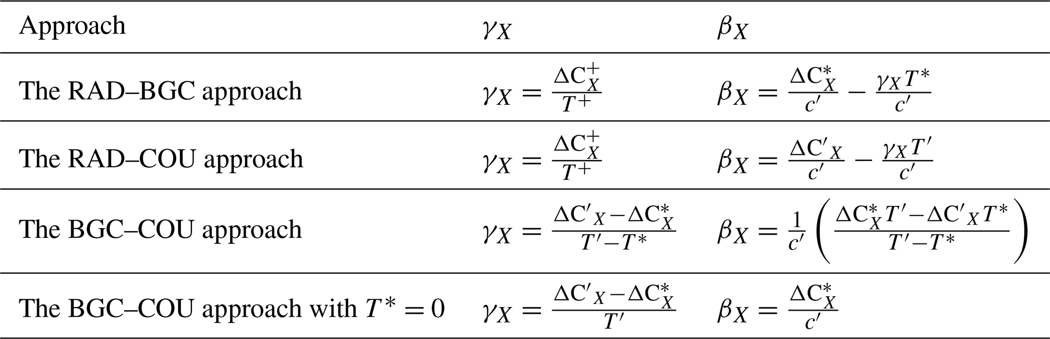
Using Eq. (1) as an example, Table 1 shows how any two combinations of the three configurations of an experiment can be used to calculate the values of the two feedback parameters. The A13 study showed that under the assumption of a linear system and if the conditions and are met, i.e. if the sum of flux and temperature changes in the RAD and BGC simulations is the same as that in the COU simulation, then all approaches yield exactly the same solution. However, this is not the case because of the nonlinearities involved (Gregory et al., 2009; Zickfeld et al., 2011; Schwinger et al., 2014).
The use of BGC and RAD simulations that have only biogeochemistry or radiative forcing responding to increases in [CO2] to find the feedback parameters is attractive since these simulations were designed to isolate the feedbacks. In the RAD simulation (whose purpose is to quantify the carbon–climate feedback, γX) the preindustrial global carbon pools for both land and ocean typically decrease in response to an increase in global temperature (hence the positive carbon–climate feedback and the negative value of γX). Consequently, negative values of γX (positive carbon–climate feedback) are obtained when using the RAD–BGC and RAD–COU approaches (see Table 1). If, however, γX is determined using the BGC and COU simulations in both of which the globally summed carbon pools for land and ocean are increasing in response to increasing [CO2], the calculated value of γX is different than that obtained using the RAD–BGC and RAD–COU approaches. In the ocean, the RAD simulation mainly measures the loss of near-surface carbon owing to warming of the surface ocean layer (Schwinger et al., 2014). The RAD simulation misses the suppression of carbon drawdown to the deep ocean due to weakening ocean circulation, because there is no buildup of a strong carbon gradient from the surface to the deep ocean in contrast to the BGC and COU simulations. Therefore, the absolute value of γX for the ocean is smaller (less negative) when calculated using the RAD–BGC and RAD–COU approaches compared to the BGC–COU approach (Schwinger et al., 2014). Over land, in the RAD simulation carbon is lost in response to increasing temperatures primarily due to an increase in heterotrophic respiration. However, an increase in temperature also potentially increases photosynthesis at high latitudes, and this increase compensates for carbon lost due to increased heterotrophic respiratory losses, especially in the presence of continuously increasing [CO2] seen in the COU configuration. Therefore γX value for land calculated using RAD–BGC and RAD–COU approaches may be higher or lower than that calculated using the BGC–COU approach. These are some mechanisms that lead to nonlinearities. Since the ongoing climate change (predominantly caused by increasing [CO2]) is best characterized by the COU simulation, it can be argued that feedback parameters are more representative when calculated using the BGC–COU approach. Here, we propose to use the COU and BGC configurations of an experiment as the standard set from which to calculate the feedback parameters as recommended in the C4MIP protocol (Jones et al., 2016). However, we also quantify the values of feedback parameters when using the RAD simulation for comparison. The calculated values of the carbon–concentration feedback parameter (βX), in contrast, are less sensitive to the approach used as shown in A13.
There is no broad consensus on whether temperature change in the BGC simulation should be assumed to be zero () as standard practice when calculating the strengths of the feedbacks, as it was in F06. While the globally averaged value of T∗ is an order of magnitude smaller than T′, the spatial pattern of T∗ is quite different from that of T′. The spatial pattern of temperature change in the COU simulation (T′) is dominated by radiative forcing of increased [CO2] with greater warming at high latitudes and over land than over ocean. In contrast, the spatial pattern of temperature change in the BGC simulation (T∗) is determined primarily by the reduction in latent heat flux associated with stomatal closure as [CO2] increases which reduces transpiration from vegetation (Bounoua et al., 1999; Ainsworth and Long, 2005). This process leads to a much more spatially variable pattern of temperature change (than T′) and the associated changes in precipitation patterns due to soil moisture–atmosphere feedbacks (Chadwick et al., 2017; Skinner et al., 2017). The difference in spatial patterns of temperature and precipitation change in the RAD versus the COU simulation is another reason that the values of the carbon–climate feedback (γX) depend on the simulation used, and this is another pathway through which nonlinearities can occur. A complete analysis of the effect of differences in spatial patterns of climate change and the carbon state on the calculated value of γX when using the RAD versus the COU simulation and determining whether or not the assumption of should be a standard practice are beyond the scope of this study but remain topics for additional scientific investigation. In the interim, we report here values of βX and γX both by considering T∗ and by ignoring it (i.e. ) when using the BGC–COU approach.
Following Table 1, when using results from the BGC and the COU configurations of a specified-concentration experiment, the values of the feedback parameters are written as
Equations (2) and (3) may be rearranged to explicitly calculate the effect of the assumption on calculated values of feedback parameters, as shown in Eqs. (4) and (5). Here, the T∗ term is retained only in the second part of the equations, whose contribution becomes zero when T∗ is ignored.
Finally, in regard to other external forcings such as nitrogen (N) deposition that directly affect carbon fluxes, the C4MIP protocol for CMIP6 (Jones et al., 2016) recommended performing additional simulations for BGC and COU versions of the 1pctCO2 experiment with time-varying N deposition in addition to their standard versions which keep N deposition rates at their preindustrial level. Simulations with N deposition can only be performed for models that explicitly model the N cycle and its interactions with the carbon (C) cycle. The rationale for recommending increasing N deposition, in conjunction with temperature and CO2 increases, is to be able to quantify the response of feedback parameters to this third forcing. However, here we restrict ourselves to the traditional analysis that considers the climate and CO2 forcings only. We do highlight, however, which models include coupled C–N cycle interactions over land. The analysis of runs with N deposition forcing is left for future studies.
2.1 Reasons for differences in feedback parameters among models
As shown later in this paper, the contribution of the second term involving T∗ in expressions for the carbon–concentration (βX) and carbon–climate (γX) feedback parameters (in Eqs. 4 and 5, when using the BGC–COU approach) is around 1 % to 5 %. This allows for the reasons for differences in the feedback parameters to be investigated across models as the expressions for the feedback parameters can be simplified in terms of the changes in the sizes of carbon pools ( and ), the temperature change in the COU simulation (T′), and the specified change in [CO2] (c′) as follows:
2.1.1 Land
Over land, Eqs. (6) and (7) can be expanded to investigate, firstly, the contributions, from changes in live vegetation pools (ΔCV) and dead litter plus soil carbon pools (ΔCS) to the strength of the feedback parameters, since . Secondly, Eq. (6) can be further decomposed to gain insight into the reasons for differences across models, in a manner similar to Hajima et al. (2014).
The superscript ∗ in Eq. (8) implies that the terms are calculated here using the BGC version of the 1pctCO2 experiment. In Eq. (8), ΔNPP and ΔGPP represent the change in net primary productivity (NPP) and gross primary productivity (GPP), ΔLF the change in litterfall flux, and ΔRh the change in heterotrophic respiration, compared to the preindustrial control experiment. The multiplicative terms in Eq. (8) do indeed have physical meaning although they are based on change in the magnitude of quantities as opposed to their absolute magnitudes. We note here explicitly that as such, these terms cannot be compared directly to the terms which are based on absolute magnitudes.
The term (fraction) is the fraction of GPP (above its preindustrial value) that is turned into NPP after autotrophic respiratory losses are taken into account. We use the term carbon use efficiency (CUE) but subscripted by Δ (CUEΔ) to represent . The subscripted Δ allows CUEΔ to be differentiated from CUE as used in the existing literature (Choudhury, 2000), which represents the fraction of absolute GPP that is converted to NPP rather than its change over some time period, as well as the point that we consider globally integrated rather than locally derived quantities. Similarly, the term represents a measure of turnover or residence timescale of carbon in the vegetation pool (τvegΔ, years). The term (PgC yr−1 ppm−1) is a measure of the strength of the globally integrated CO2 fertilization effect. However, in the models that dynamically simulate changes in vegetation cover, the effect of changes in vegetation coverage is implicitly included in this term. The term is a measure of the average residence time of carbon in the dead litter and soil carbon pools (τsoilΔ, years). However, as with CUE, this quantity cannot be compared directly to the residence time of carbon in the litter plus soil carbon pool calculated using the absolute values of CS and Rh. Nor can it be compared to the changes in carbon residence time due to the “false priming effect” associated with the increase in NPP inputs, as [CO2] increases, into the dead carbon pools (Koven et al., 2015). (fraction) is a measure of the increase in heterotrophic respiration per unit increase in litterfall rate, and (PgC yr−1 ppm−1) indicates the global increase in litterfall rate per unit increase in CO2, which in principle, should be close to the change in net primary productivity per unit increase in CO2, . A comparison of these terms across models can potentially yield insight into the reasons for large differences in land carbon uptake across models.
2.1.2 Ocean
Assuming changes in the biological organic carbon inventory are small, the change in the ocean carbon inventory, ΔCO, is defined by an integral of the change in the dissolved inorganic carbon, ΔDIC, and density over the ocean volume:
where ΔCO is in petagrams of carbon; the ocean dissolved inorganic carbon, DIC, is in moles per cubic meter; the ocean volume V is in cubic meters; and the multiplier 10−15 converts grams to petagrams of carbon.
To gain insight into how the ocean carbon distribution is controlled, the ocean dissolved inorganic carbon, DIC, may be defined in terms of separate carbon pools (Ito and Follows, 2005; Williams and Follows, 2011; Lauderdale et al., 2013; Schwinger and Tjiputra, 2018):
where the preformed carbon, DICpreformed, is the amount of carbon in a water parcel when in the mixed layer at the time of subduction and the regenerated carbon, DICregenerated, is the amount of dissolved inorganic carbon accumulated below the mixed layer due to the biological regeneration of organic carbon. The preformed carbon is affected by the carbonate chemistry and ocean physics. To gain further insight into how close the ocean is to an equilibrium with the atmosphere, the preformed carbon, DICpreformed, is further split into saturated, DICsat, and disequilibrium, DICdisequilib, components. The saturated component represents the concentration in surface water fully equilibrated with the contemporary atmospheric CO2 concentration. The disequilibrium component represents the extent that surface water is incompletely equilibrated before subduction, which is affected by the strength of the ocean circulation altering the residence time in the mixed layer and the ocean ventilation rate. Each of these components is affected by the increase in atmospheric CO2 and the changes in climate.
The change in the global ocean carbon inventory, ΔCO, relative to the preindustrial period may then be related to the global volume integral of the change in each of these DIC pools:
where ΔCpreformed is the preformed carbon inventory, ΔCsat is the saturated carbon inventory, ΔCdisequilib is the disequilibrium carbon inventory, and ΔCregenerated is the regenerated carbon inventory.
The simplified expressions for carbon cycle feedback parameters in Eqs. (6) and (7) based on the air–sea flux changes to the ocean may then be approximated by the global ocean carbon inventory changes, which may be expressed in terms of these different global ocean carbon pools (Williams et al., 2019):
The anomalies for each of these carbon pools are calculated as
where RCO and RNO are constant stoichiometric ratios, ΔAOU is the change in apparent oxygen utilization from its preindustrial value (where preformed oxygen is assumed to be approximately saturated with respect to atmospheric oxygen); ΔAlk is the change in alkalinity; To and So are the ocean temperature and salinity, respectively; P and Si are the phosphate and silicate concentrations; and ΔAlkpre is the change in preformed alkalinity (Ito and Follows, 2005; Williams and Follows, 2011; Appendix of Lauderdale et al., 2013). In Eq. (16), ΔDICsat is calculated using the partial pressure of CO2 in the atmosphere (p) and preformed alkalinity as represented by the function f following the iterative solution for the ocean carbon system of Follows et al. (2006) and by considering the small contribution of minor species (borate, phosphate, silicate) to the preformed alkalinity, at time t, and the preindustrial values, at time t=0. In Eq. (16), the calculation uses the preformed alkalinity, the alkalinity at the time of water subduction, instead of the total instantaneous alkalinity to remove the effect of CaCO3 dissolution from the time the water parcel lost contact with the atmosphere. The preformed alkalinity is estimated from a multiple linear regression using salinity and the conservative tracer PO (; Gruber et al., 1996), with the coefficients of this regression estimated based on the upper ocean (first 10 m) alkalinity, salinity, oxygen, and phosphate in each model. Our diagnostics of the ocean feedbacks and carbon pools depend primarily upon changes in DIC and upon the preformed and regenerated pools, relative to the preindustrial period, although differences in the preindustrial ocean in our suite of models do affect the saturated DIC changes relative to the preindustrial period by ∼5 % or less due to the nonlinearity of the carbonate chemistry.
Table 2Primary features of the physical atmosphere and ocean components and land and ocean carbon cycle components of the 11 participating models in this study.
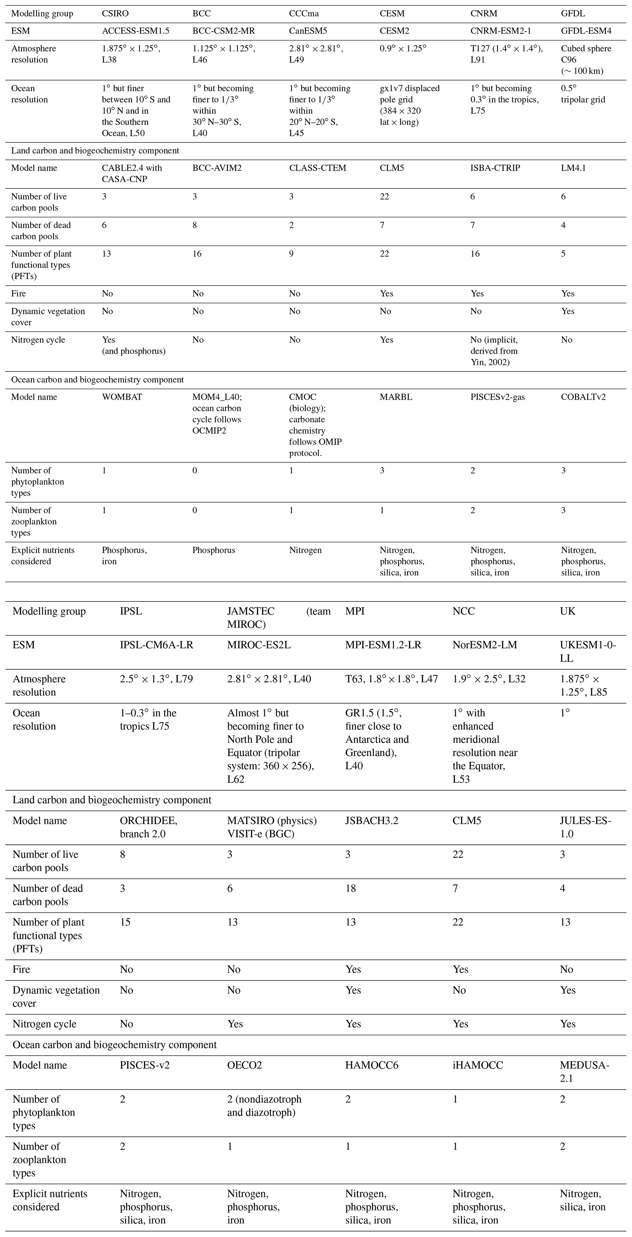
Table 2 summarizes the primary features of the 11 comprehensive ESMs that contributed results to this study. Brief descriptions of land and ocean carbon cycle components of these ESMs are provided in the Appendix. The 11 ESMs, in alphabetical order, are the (1) Commonwealth Scientific and Industrial Research Organisation (CSIRO) ACCESS-ESM1.5, (2) Beijing Climate Center (BCC) BCC-CSM2-MR, (3) Canadian Centre for Climate Modelling and Analysis (CCCma) CanESM5, (4) Community Earth System Model version 2 (CESM2), (5) Centre National de Recherches Météorologiques (CNRM) CNRM-ESM2-1, (6) Institut Pierre Simon Laplace (IPSL) IPSL-CM6A-LR, (7) Japan Agency for Marine-Earth Science and Technology (JAMSTEC) in collaboration with the University of Tokyo and the National Institute for Environmental Studies (team MIROC) MIROC-ES2L, (8) Max Planck Institute for Meteorology (MPI) MPI-ESM1.2-LR, (9) Geophysical Fluid Dynamics Laboratory (GFDL) NOAA-GFDL-ESM4, (10) Norwegian Climate Centre (NCC) NorESM2-LM, and (11) United Kingdom (UK) UKESM1-0-LL.
In contrast to the A13 study where only two of the eight participating comprehensive ESMs had the terrestrial N cycle implemented and coupled to their C cycle, in this study 6 of the 11 participating ESMs represent coupling of terrestrial C and N cycles. These six models are the ACCESS-ESM1.5, CESM2, MIROC-ES2L, MPI-ESM1.2-LR, NorESM2-LM, and UKESM1-0-LL. Note that CESM2 and NorESM2-LM employ the same land surface component – version 5 of the Community Land Model (CLM5) – so we expect the land carbon cycle to respond very similarly in the two models. Three of the ESMs have land components that dynamically simulate vegetation cover and competition between their PFTs – NOAA-GFDL-ESM4, MPI-ESM1.2-LR, and UKESM1-0-LL.
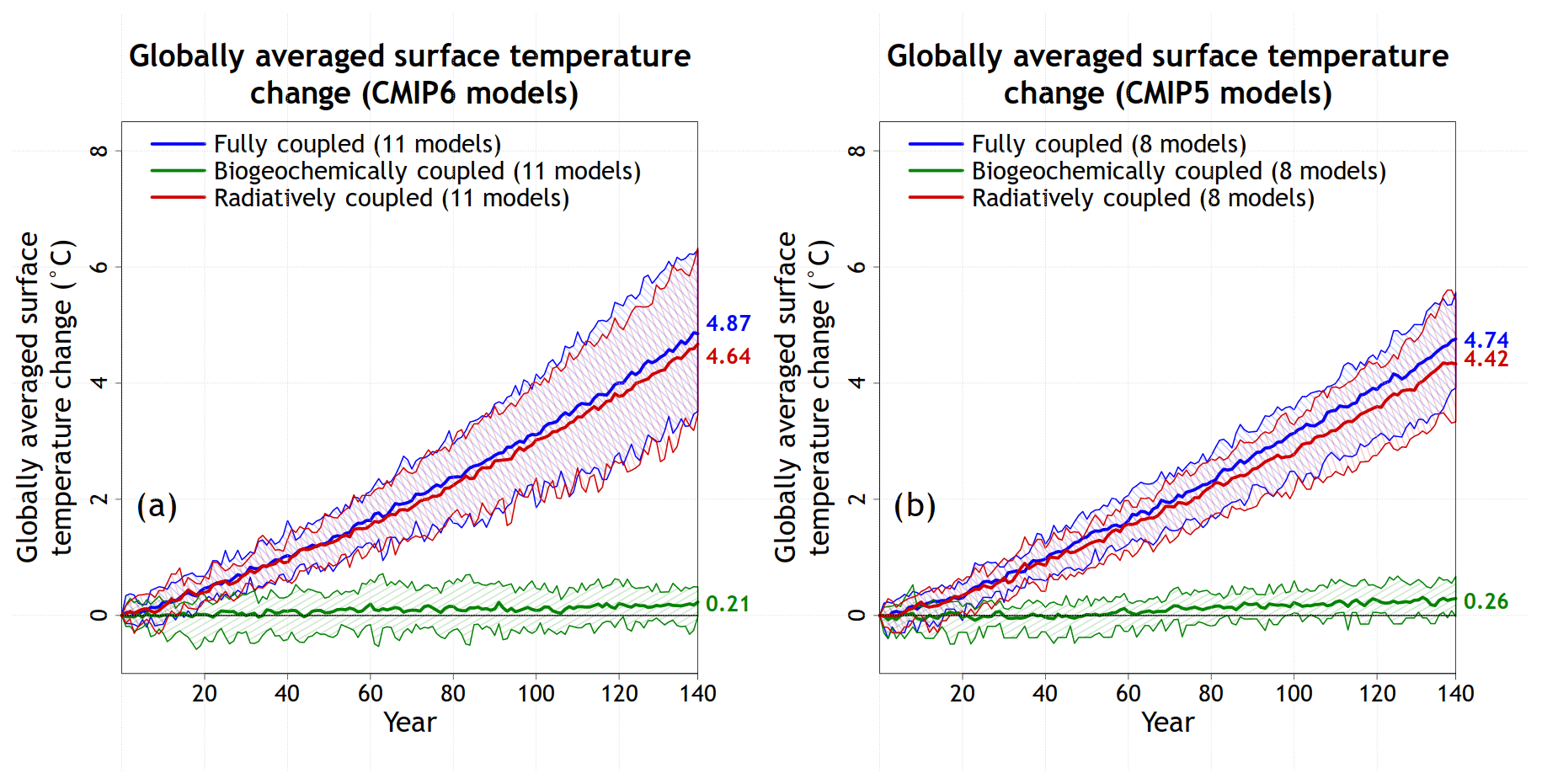
Figure 1Temperature changes in the fully, biogeochemically, and radiatively coupled configurations of the 1pctCO2 experiment across participating CMIP6 (a) and CMIP5 (b) comprehensive ESMs that participated in this and the A13 study, respectively. The model mean is indicated by the solid lines, and the range across the models is indicated by shading around the solid lines. Individual CMIP6 model results are shown in Fig. A1 in the Appendix.
4.1 Global surface CO2 fluxes and temperature change
Figure 1 shows the simulated changes in temperature in the three model configurations (COU, BGC, and RAD) of the 1pctCO2 experiment. Here and in subsequent figures, results are also shown for the eight comprehensive ESMs that participated in the A13 study. The eight models in the A13 study are a subset of 11 models considered in this study although they have been updated since CMIP5.
As expected, temperature change is higher in the COU and RAD simulations than in the BGC simulation, since the radiative forcing responds to increasing [CO2] in these simulations. The small temperature change in the BGC simulation is due to a number of not only contributing but also compensating factors: (1) reduction in transpiration and hence latent heat flux due to stomatal closure in response to increasing [CO2] (Cao et al., 2010); (2) increase in vegetation leaf area index (LAI), which decreases land surface albedo and hence increases absorbed solar radiation; and (3) increase in vegetation fraction in models that explicitly simulate competition between their plant functional types (PFTs) over land (NOAA-GFDL-ESM4, MPI-ESM1.2-LR, and UKESM1-0-LL), which also leads to reduced land surface albedo. As a result, temperature change in the COU simulation is higher than in the RAD simulation since these biogeochemical processes are active and contribute to a small additional warming. This is seen in Fig. 1a for CMIP6 models and Fig. 1b for CMIP5 models.
When comparing CMIP5 and CMIP6 models, the CMIP6 models are on average slightly warmer than CMIP5 models in the COU and RAD simulations. In Fig. 1a, the globally averaged near-surface temperature change at CO2 quadrupling in the COU simulation is 4.87 ∘C in CMIP6 models, compared to 4.74 ∘C in CMIP5 models. The CMIP6 ensemble considered here includes some high-climate-sensitivity models including CanESM5, CESM2, CNRM-ESM2-1, IPSL-CM6A-LR, and UKESM1-0-LL. The globally averaged temperature change at CO2 quadrupling in the COU simulation for the eight models that are common to this (CMIP6) and the A13 (CMIP5) studies is 4.97 and 4.74 ∘C, respectively. The temperature change in the BGC simulation in CMIP6 models (0.21 ∘C) is, however, slightly lower than in the CMIP5 models (0.26 ∘C). The values in Fig. 1 for participating CMIP5 models are slightly different than those reported in the A13 study because those numbers also included the UVic Earth System Climate Model (an intermediate complexity model), which we have omitted here to keep the comparison consistent between comprehensive ESMs. In addition, in contrast to A13, the temperature at the end of the simulations in this study is calculated after fitting a fourth-order polynomial in R to the model mean values rather than using the actual model mean value at the end of the simulation which can be higher or lower than that calculated using the polynomial fit due to interannual variability. A fourth-order polynomial fit has been shown to yield a good estimate of the forced response of the global mean temperature response and to minimize the potential influence of internal variability (Hawkins and Sutton, 2009).
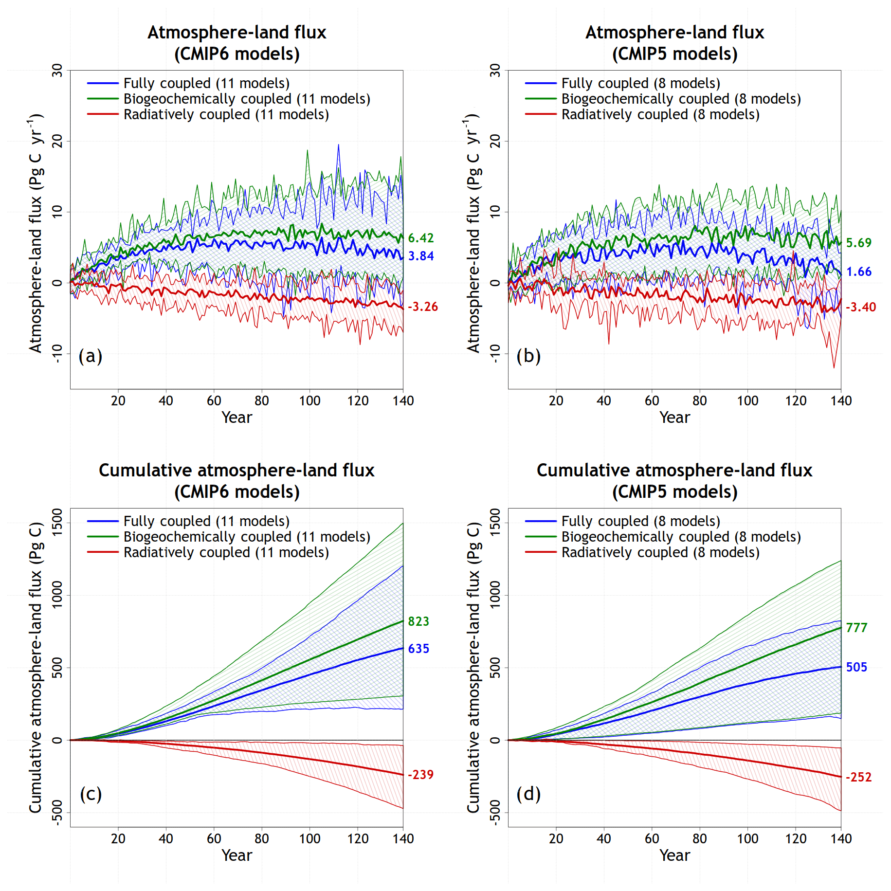
Figure 2Model mean values and the range across models for annual simulated atmosphere–land CO2 flux (a, b) and their cumulative values (c, d) for participating CMIP6 (a, c) and CMIP5 (b, d) models from the fully, biogeochemically, and radiatively coupled versions of the 1pctCO2 experiment. Individual CMIP6 model results are shown in Fig. A1.
Figures 2 and 3 show simulated model mean values and the range across models for annual simulated atmosphere–land and atmosphere–ocean CO2 fluxes and their cumulative values for participating CMIP6 and CMIP5 models from the COU, BGC, and RAD configurations of the 1pctCO2 experiment. The general results from CMIP6 models are broadly similar in nature to those from CMIP5 models, as would be expected, with higher annual and cumulative values of atmosphere–land and atmosphere–ocean CO2 fluxes in the BGC simulation compared to the COU simulation in which the radiative warming caused by increasing CO2 weakens the land and ocean sinks. In the RAD simulation, where land and ocean carbon cycle components do not respond to increasing [CO2], both components lose carbon, for reasons discussed below.
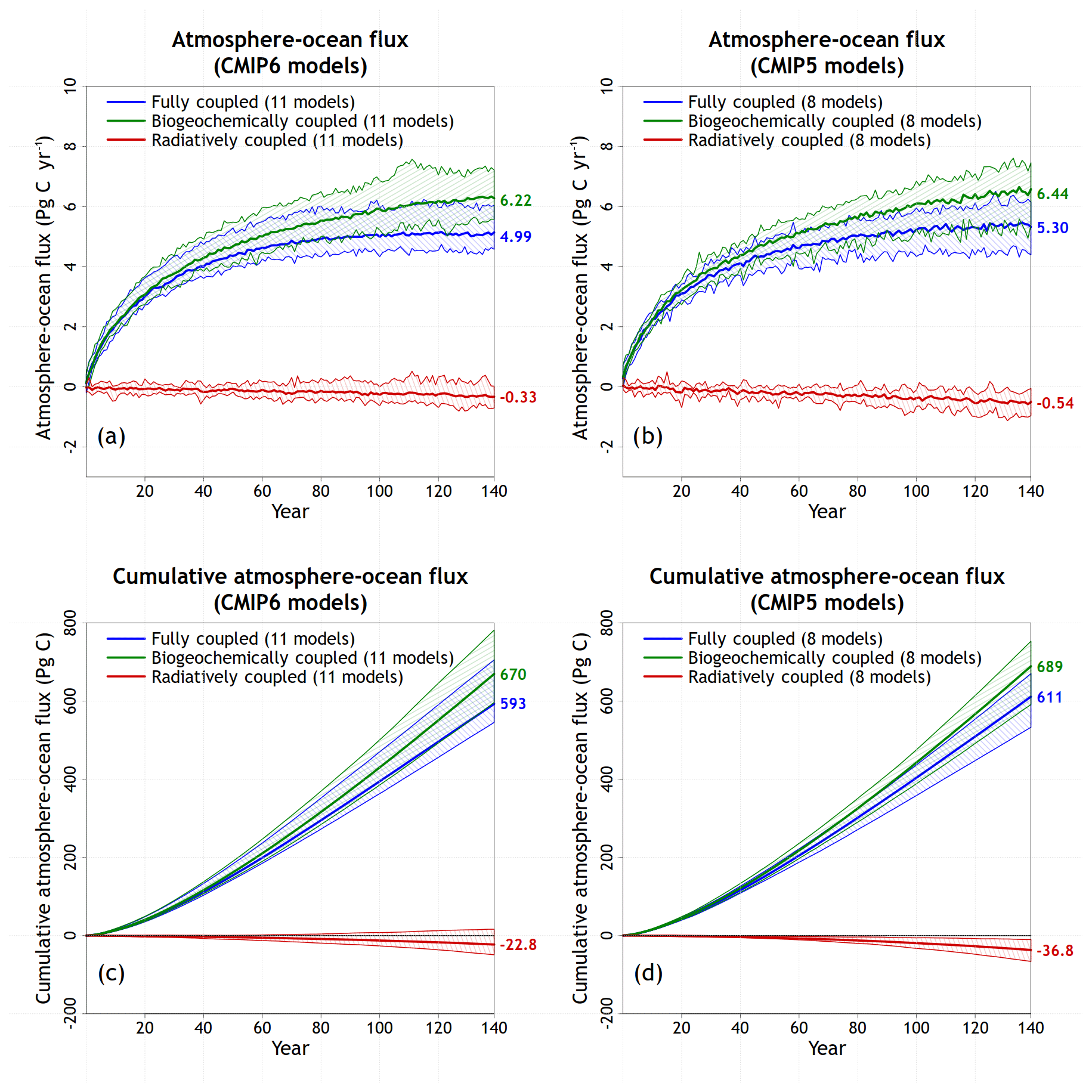
Figure 3Model mean values and the range across models for annual simulated atmosphere–ocean CO2 flux (a, b) and their cumulative values (c, d) for participating CMIP6 (a, c) and CMIP5 (b, d) models from the fully, biogeochemically, and radiatively coupled versions of the 1pctCO2 experiment. Individual CMIP6 model results are shown in Fig. A1.
Over land, the model mean rate of increase in atmosphere–land CO2 flux declines and even becomes negative in the COU and BGC simulations as the terrestrial CO2 fertilization effect saturates and the carbon pools build up, which increases the respiratory losses. The biggest difference between the CMIP5 and CMIP6 models is that the cumulative land carbon uptake in the COU simulation is about 25 % higher in CMIP6 (635 ± 258 PgC, mean ± standard deviation) models than in CMIP5 (505 ± 297 PgC) models, although this increase is not statistically significant across the model ensemble (Mann–Whitney test). Here and hereafter, we use the sample (not population) standard deviation. The cumulative value of carbon loss in the RAD simulation is similar in both CMIP6 and CMIP5 models: 239 ± 120 vs. 252 ± 158 PgC, respectively. This carbon loss occurs due to both increased heterotrophic respiration per unit carbon mass and reduced GPP (and consequently NPP) in the RAD simulation (not shown). While NPP declines globally in response to increases in temperature, mid- to high-latitude net primary production increases (Qian et al., 2010), so the reduction in global NPP comes largely from the reduction in the tropics. The large spread across CMIP6 land carbon cycle models, seen also in earlier F06 and A13 studies, has not changed significantly compared to CMIP5 models, and its implications will be discussed in more detail in Sect. 5. As discussed later in Sect. 4.3, the standard deviation of land carbon–climate feedback increases from CMIP5 to CMIP6 models, while it decreases somewhat for the land carbon–concentration feedback.
Over the ocean, the response to increasing [CO2] and changing climate remains fairly similar across CMIP5 and CMIP6 models. The cumulative ocean carbon uptake in the COU simulation is 593 ± 54 and 611 ± 50 PgC in CMIP6 and CMIP5 models, respectively. Unlike the land uptake, however, the ocean carbon uptake does not saturate over the length of the simulation in the BGC simulation (Fig. 3a, b); it keeps on increasing albeit at a declining rate. The cumulative ocean carbon loss in the RAD simulation is 23 ± 19 and 37 ± 17 PgC in CMIP6 and CMIP5 models, respectively, and is primarily associated with warmer temperatures which reduce CO2 solubility (Goodwin and Lenton, 2009; Schwinger et al., 2014).
As in F06 and A13, the range in cumulative atmosphere–land CO2 fluxes among models at the end of the COU simulation, in response to changes in atmospheric CO2 concentration and surface temperature, is 3 to 4 times larger than for the atmosphere–ocean CO2 fluxes. Figure A1 shows results from individual CMIP6 models for which model means and ranges were shown in Figs. 1, 2, and 3 and allows for the identification of models which behave differently compared to the majority of models.

Figure 4Components of the carbon budget terms in cumulative emissions from the 11 participating CMIP6 models based on Eq. (A6) in (a) and Eq. (A7) in (b) using results from the fully coupled 1pctCO2 simulation. The models are arranged in an ascending order based on their cumulative emissions values. Results from participating CMIP5 models in the A13 study are shown in panels (c) and (d). In addition, ESMs whose land component includes a representation of the N cycle are identified by a red font colour for cumulative land carbon uptake (a, c) and fractional emissions taken up by land (b, d). Model mean is shown not only for all models but also separately for models whose land components include or do not include a representation of the N cycle.
4.2 Carbon budget terms
Figure 4a shows the carbon budget components of the diagnosed cumulative fossil fuel emissions at the end of the 140-year period of the 1pctCO2 COU experiment when CO2 concentration quadruples ( or simply ), from CMIP6 models. Cumulative emissions can similarly also be calculated at 2×CO2 (). The term “carbon budget” in this context refers to the accounting of carbon internal to individual ESMs. The sum of ocean () and land () sinks and the resulting change in atmospheric carbon burden () yield cumulative fossil fuel emissions which are consistent with the specified CO2 pathway (the 1pctCO2 scenario in this case) as indicated in the Appendix (Eq. A6). The corollary to this is that, in a specified emissions simulation, if the respective fossil fuel emissions were to be used in their models, each model would yield CO2 concentrations that rise at a rate of 1 % yr−1. The term “diagnosed” implies that the cumulative fossil fuel emissions are calculated from changes in atmosphere, land, and ocean carbon pools in the specified-concentration 1pctCO2 experiment. Figure 4b shows the terms of the budgets as fractional components for atmosphere (A), land (L), and ocean (O) based on Eq. (A7), where fA is the airborne fraction of emissions and fL and fO are the fractions of emissions take up by land and ocean, respectively. More details are provided in Sect. A1 of the Appendix.
All panels in Fig. 4 identify models whose land component includes a representation of the N cycle – the cumulative land carbon uptake (panels a and c) and fractional emissions taken up by land (panels b and d) for these models are shown in red.
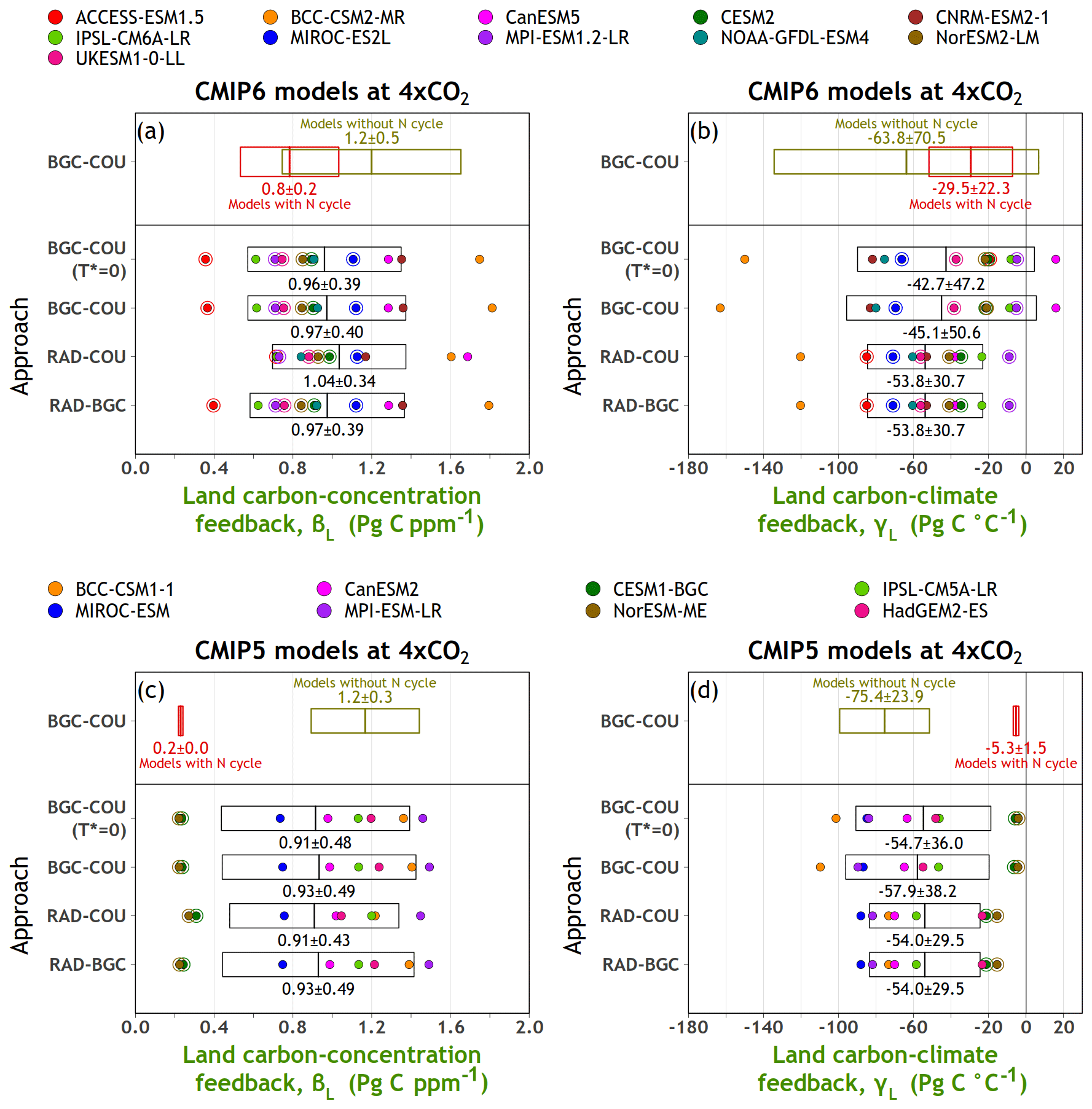
Figure 5Carbon–concentration (a) and carbon–climate (b) feedback parameters over land from participating CMIP6 models calculated using the approaches summarized in Table 1. The boxes show the mean ± 1 standard deviation range, and the individual coloured dots represent individual models. Models which include a representation of the land nitrogen cycle are identified with a circle around their dot. The model mean ± 1 standard deviation range of feedback parameters is also separately shown for models which do and do not represent the land nitrogen cycle using the BGC–COU approach. Results from participating CMIP5 models in the A13 study are shown in (c) and (d).
Consistent with Figs. 2 and 3, and CMIP5 results reported in the A13 study, the differences among models are primarily due to the diverse response of the land carbon cycle components. While the model mean cumulative carbon uptake by the ocean is fairly similar between participating CMIP5 (611 ± 50 PgC) and CMIP6 (593 ± 54 PgC) models, the land uptake is higher in CMIP6 (635 ± 258 PgC) compared to CMIP5 (505 ± 297 PgC) models, as mentioned earlier. This is the case even when the CanESM5, the model with the largest land carbon uptake, is omitted from CMIP6 models (model mean land carbon uptake for the remaining 10 models is 578 ± 185 PgC). As a result, the model mean cumulative diagnosed emissions from CMIP6 models (3031 ± 242 PgC) are about 4 % higher than those from CMIP5 models (2927 ± 294 PgC). In Fig. 5a, the land carbon uptakes in the CESM2 (656 PgC) and NorESM2-LM (652 PgC) models are very similar; as noted above these models employ the same land component. Model mean estimates that are reported separately for models whose land component does and does not include a representation of the N cycle, for both CMIP5 and CMIP6 models, show that the model mean land carbon uptake is lower for models that explicitly represent the N cycle. As a consequence, the airborne fraction of emissions is also higher for models that represent the land N cycle and their diagnosed cumulative fossil fuel emissions are lower (Fig. 4). Of the 11 CMIP6 ESMs considered in this study, 6 represent the N cycle over land compared to only 2 of the 8 considered in the A13 study based on CMIP5 models. Yet, the model mean land carbon uptake over land is higher in this study than in the A13 study. This is partly because of the three models with the largest land carbon uptake (CNRM-ESM2-1, BCC-CSM2-MR, and CanESM5) which do not include land the N cycle (Fig. 4a). In addition, inclusion of the N cycle does not universally imply lower land C uptake. In Fig. 4a, IPSL-CM6A-LR and NOAA-GFDL-ESM4, both of which do not include the land N cycle, yield lower land carbon uptake than four of the models that do include the land N cycle.
Figure 4a and c allow for the direct comparison of models from the same modelling group. CanESM2, from the CCCma, which had below-average land carbon uptake among CMIP5 models, has evolved into CanESM5, a model with the largest land carbon uptake among CMIP6 models. The reason for this is an increase in the strength of its CO2 fertilization effect following the retuning of its photosynthesis downregulation parameters, using carbon budget constraints over the historical period, as explained in Arora and Scinocca (2016). CESM1, which had one of the lowest land carbon uptakes among CMIP5 models, because of its apparently excessive nitrogen limitation effect in CLM4, has evolved into CESM2 (with the CLM5 land component) with near-average land carbon uptake among CMIP6 models. The transition of CLM from CLM4 to CLM5 on the one hand and the reduction in its nutrient constraints on photosynthesis and the parametric controls on fertilization responses on the other are discussed in Wieder et al. (2019) and Fisher et al. (2019), respectively. The land carbon uptake in MIROC-ESM increased from the lowest among CMIP5 models to near average for MIROC-ES2L among CMIP6 models, due to a new terrestrial biogeochemical component (Ito and Inatomi, 2012). Although the CO2 fertilization effect in this new land model is weaker likely due to the incorporation of the nitrogen cycle, the model yields relatively higher NPP (Hajima et al., 2020), due to a higher CUEΔ (as confirmed later in Sect. 4.4.1). The land carbon uptake in the IPSL-CM5A-LR model decreased from being the second largest in CMIP5 models to below average for the IPSL-CM6A-LR model due to the implementation of terrestrial photosynthesis downregulation, as a function of CO2 concentration, which leads to a decrease in GPP across all latitudes, with the largest decrease in the tropics. For the MPI ESM, the decrease in land carbon uptake in MPI-ESM-LR for CMIP5 and MPI-ESM1.2-LR for CMIP6 is associated with the implementation of a nitrogen cycle model (Goll et al., 2017) and a new soil carbon model Yasso (Goll et al., 2015). Compared to its predecessor HadGEM2-ES, UKESM1-0-LL represents a prognostic treatment of terrestrial nitrogen including its impact on carbon storage in vegetation biomass and soil organic matter. A limitation on terrestrial productivity from available nitrogen is likely also the main reason for reduced land carbon storage in UKESM1-0-LL compared to in HadGEM2-ES.
The ocean carbon uptake in the IPSL model decreased from being the largest among CMIP5 models in IPSL-CM5A-LR to being lower than average for IPSL-CM6A-LR, and this change is attributed to a greater ocean stratification in the IPSL-CM6A-LR. The annual mean mixed-layer depth is 46.7 and 40.2 m in IPSL-CM5A-LR and IPSL-CM6A-LR, respectively. While NorESM1-ME was one of the CMIP5 models with the largest ocean carbon uptake, NorESM2-LM has an ocean carbon uptake close to the CMIP6 model mean. This change is a consequence of changes in the simulated (shallower depth and weaker strength) Atlantic meridional overturning circulation and reduced mixed-layer biases particularly at high latitudes (less deep winter mixing). Due to these modifications, the efficiency of carbon export below the mixed layer in NorESM2-LM is considerably reduced compared to in NorESM1-ME. This, in turn, leads to less excess carbon stored in the North Atlantic Deep Water (below 2000 m) as well as in the Antarctic Intermediate Water.
Figure A2 in the Appendix shows a version of Fig. 4 but at the time of CO2 doubling (at year 70). Interestingly, the ordering of the models according to their diagnosed cumulative emissions at 2×CO2 is different from that at 4×CO2. As expected, however, the model mean fractional emissions taken up by land and ocean at 2×CO2 are higher than at 4×CO2, because both land and ocean carbon sinks relatively weaken as CO2 continues to increase.
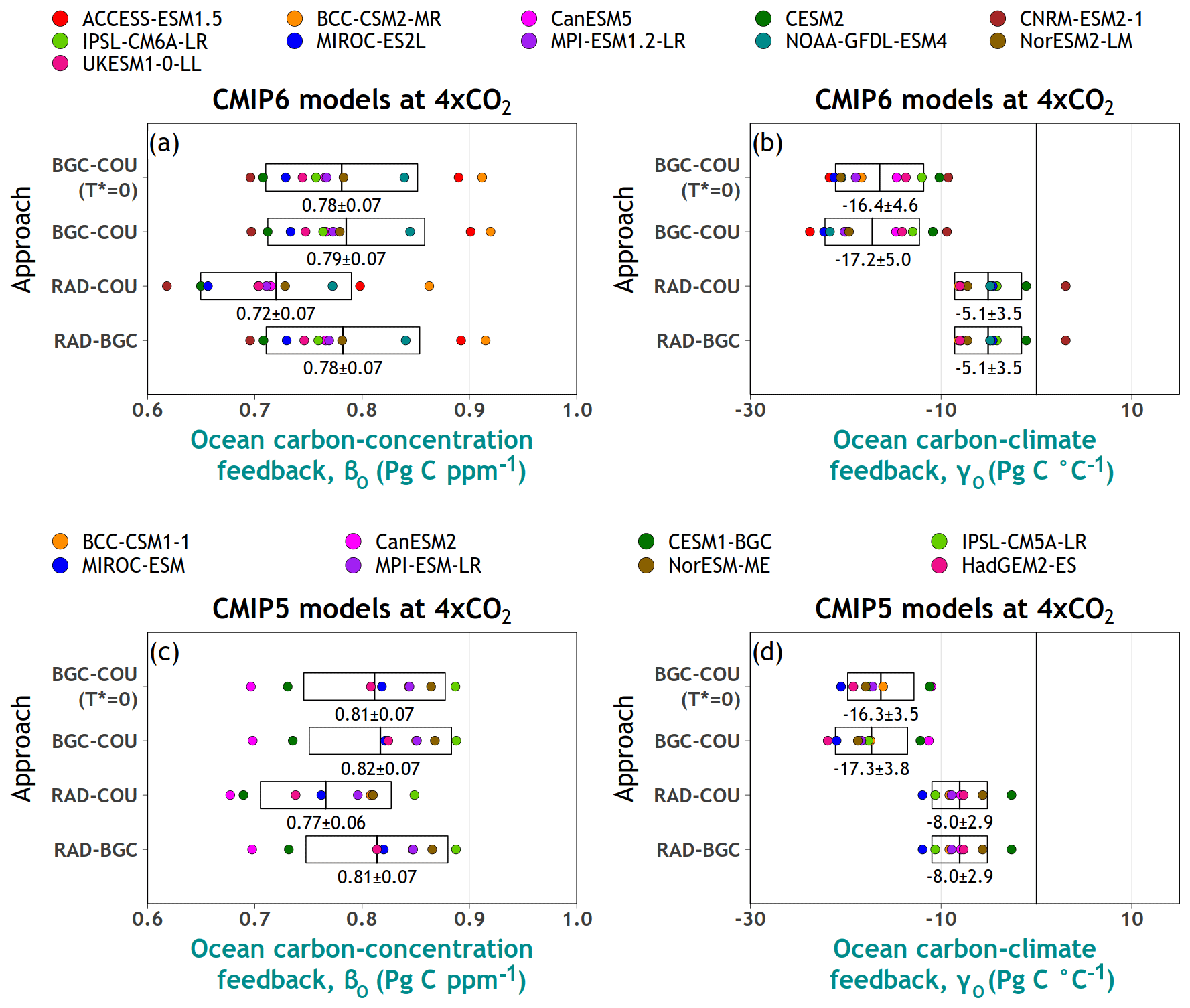
Figure 6Carbon–concentration (a) and carbon–climate (b) feedback parameters over ocean from participating CMIP6 models calculated using the approaches summarized in Table 1. The boxes show the mean ± 1 standard deviation range. Results from participating CMIP5 models in the A13 study are shown in (c) and (d).
4.3 Feedback parameters
Figure 5a and b compare the carbon–concentration feedback (βL) and carbon–climate feedback (γL) parameters over land from participating CMIP6 models, calculated using results at the end of the BGC, RAD, and COU simulations. The plots show not only feedback parameters from different models as coloured dots but also their mean ± 1 standard deviation as a box. Three primary observations can be made from Fig. 5. First and foremost, the spread in the magnitude of the carbon–concentration and carbon–climate feedback over land in CMIP6 models is of a similar magnitude to that in CMIP5 models (Fig. 5c and d). Second, the carbon–climate feedback (γL) is more sensitive to the approach used (and hence the type of simulations used) to derive its value than the carbon–concentration feedback (βL). The absolute value of βL varies by around 7 %, while γL varies by up to 26 %, depending on the approach used. Third, in the model mean sense, the absolute strength of the feedback parameters is weaker for models that include a representation of the N cycle, for both CMIP5 and CMIP6 models. Both the carbon gain due to an increase in atmospheric CO2 concentration and the carbon loss due to an increase in the global average temperature in models with representation of the land N cycle are much lower than in models that do not include the N cycle. This response is most likely explained by the N limitation of photosynthesis as CO2 increases and the additional release of N from dead organic matter as warming increases, which boosts productivity, thereby compensating for carbon lost due to increased respiratory losses, as also discussed in A13. The values of the feedback parameters, however, overlap between models that do and do not include a representation of the N cycle, given the wider spread in the feedback parameter values among models that do not include a representation of the land N cycle compared to models that do.
Figure 6a and b compare the carbon–concentration feedback (βO) and carbon–climate feedback (γO) parameters over the ocean from participating CMIP6 models. For both CMIP5 and CMIP6 models, the absolute spread in the magnitude of the feedback parameters across the participating models is an order of magnitude smaller for the ocean C cycle component compared to the land C cycle component, as was also seen in F06 and A13. Similar to the land, the calculated values of the ocean carbon–climate feedback (γO) are more sensitive to the approach used (and hence the type of simulations used) than the ocean carbon–concentration feedback (βO). In agreement with Schwinger et al. (2014), the absolute values of γO are 2–3 times larger when calculated using the COU and BGC simulations, compared to cases when RAD simulation is used, for reasons mentioned earlier. Figures 5 and 6 show also that while the strength of the carbon–concentration feedback is similar over land and ocean, the strength of the carbon–climate feedback parameter over ocean is much weaker than over land.
Figures 5 and 6 provide justification for using the BGC–COU approach, over the RAD–BGC and RAD–COU approaches, in calculating the feedback parameters as discussed below. In Fig. 6, the absolute magnitude of γO when using the BGC–COU approach is about twice as large in CMIP5 models and more than 3 times larger in CMIP6 models compared to its model mean value calculated using the RAD–BGC and RAD–COU approaches. The reason for this is that the RAD simulation misses the suppression (due to weakening of the ocean circulation) of carbon drawdown to the deep ocean due to a lack of buildup of a strong carbon gradient from the atmosphere to the deep ocean, as mentioned earlier. This process is important when climate change is forced by increasing atmospheric CO2, and therefore feedback parameters calculated using the BGC–COU approach are more likely to include all processes relevant to application to realistic scenarios. In Fig. 6, the value of γO changes sign for the CNRM-ESM2-1 model from positive when calculated using the RAD–BGC or RAD–COU approaches to negative when calculated using the BGC–COU approach, and this further illustrates the sensitivity of feedback parameters to the approach used to calculate them. Section A2 discusses the reasons for this sensitivity in the CNRM-ESM2-1 model.
In Fig. 5, although the carbon–climate feedback parameter over land (γL) is larger in absolute terms, it is comparatively less sensitive to the approach used than that over ocean, because over land an increase in temperature not only increases the respiratory losses but also affects photosynthetic processes especially in conjunction with increasing CO2. Warmer temperatures increase photosynthesis over mid- to high-latitude regions where photosynthesis is currently limited by temperature and more so with increasing CO2 but decrease photosynthesis over tropical regions where the temperatures are already too warm for optimal photosynthesis. The net result of these compensating processes plays out very differently in different models, and in the model mean sense this results in less sensitivity over land than over ocean of the calculated value of the carbon–climate feedback parameter (γL and γO, respectively) to the different approaches. This is seen in both CMIP5 and CMIP6 models. Over land, photosynthesis is also affected by temperature (with widely varying responses between models) in addition to respiration, and the γL values vary widely between models between the RAD–BGC and RAD–COU approach and the BGC–COU approach. This is seen, for example, for the ACCESS-ESM1.5, IPSL-CM6A-LR, and CanESM5 models in Fig. 5b.
Figures 5 and 6 also show that the effect of assuming T∗ (the temperature change in the BGC simulation) to be zero is around 1 % for the calculated value of the carbon–concentration feedback parameter () and around 5 % for the carbon–climate feedback parameter (). This small effect of T∗ on the calculated global values of the feedback parameter allows for the investigation of the reasons for differences among model by using simplified forms of βX and γX as presented in Eqs. (6) and (7).
For completeness, Table A1 in the Appendix summarizes the values of feedback parameters for both land and ocean from CMIP6 and CMIP5 models (corresponding to Figs. 5 and 6) not only at 4×CO2 but also at 2×CO2. Table A1 also shows the value of parameter α, the linear transient climate sensitivity to CO2, following F06 (their Eq. 6), which is calculated using values at the end of the COU simulation as
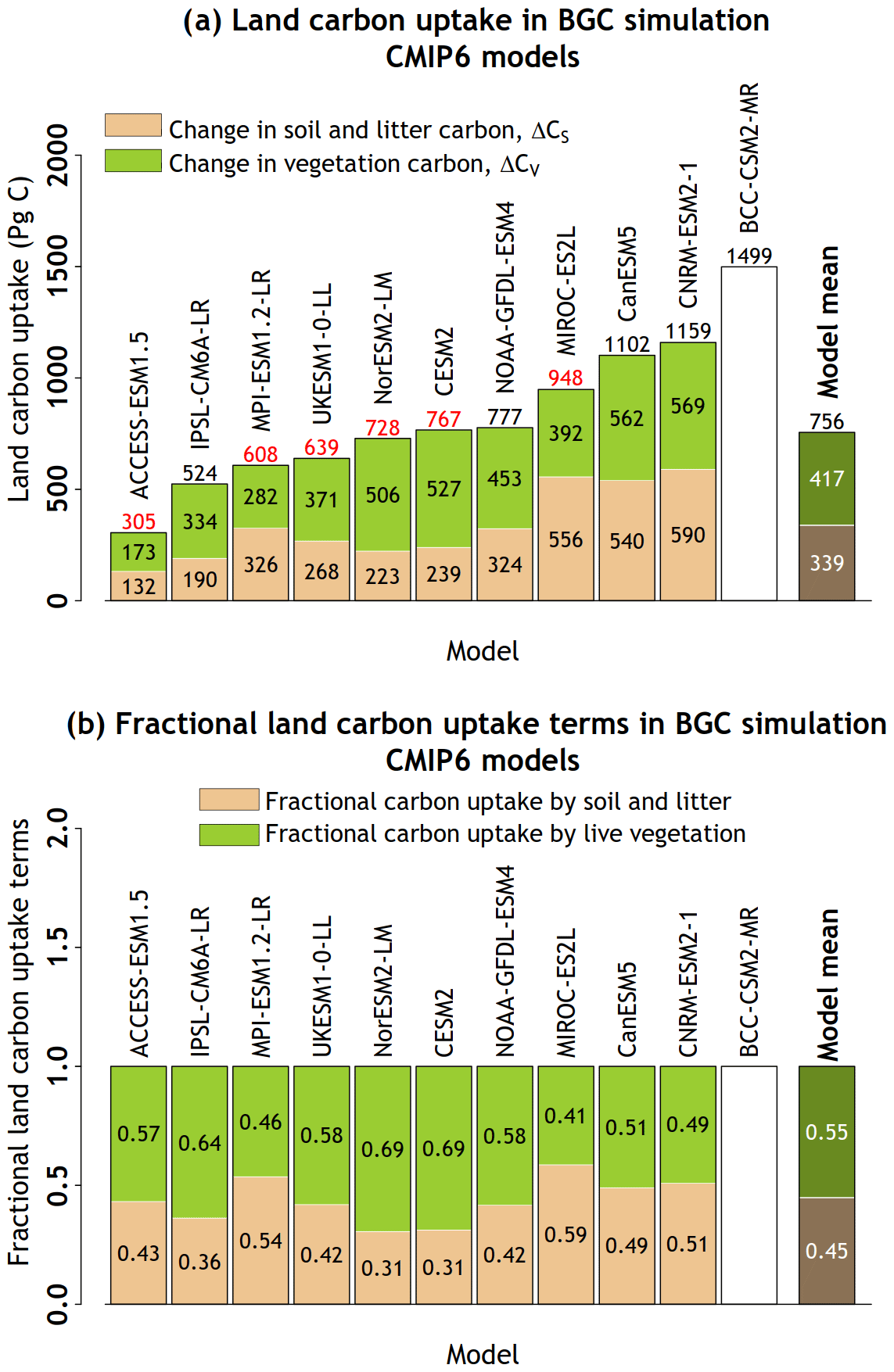
Figure 7Carbon uptake over land in the BGC simulation, used to calculate land carbon–concentration feedback (βL) and its partitioning into vegetation and soil + litter carbon pools across the participating CMIP6 models (a). Panel (b) shows the fractional land carbon uptake by vegetation and soil + litter carbon pools in the BGC simulation. No partitioning is shown for the BCC-CSM2-MR model because total land carbon uptake in this model exceeded the sum of changes in the vegetation and soil + litter carbon pools by more than 10 %. Total land carbon uptake in models which include a representation of the N cycle is shown in red. The results from the BCC-CSM2-MR model are not used in calculating the model mean values.
4.4 Reasons for differences among models
4.4.1 Land
Equations (8) and (9) in Sect. 2.1.1 are used to gain insight into reasons for differing responses of land models. In the BGC–COU approach and assuming (Eq. 8), the carbon uptake in the BGC simulation is used to calculate the carbon–concentration feedback parameter (βL). Figure 7 shows how this carbon uptake over land is separated into vegetation and soil + litter components both in absolute (panel a) and fractional (panel b) terms. Figure 7b shows that models vary widely in terms of how the carbon uptake over land is split into vegetation and soil + litter components. The model mean values indicate that slightly more of the carbon sequestered is allocated to vegetation (55 %) than to the soil + litter pools (45 %).
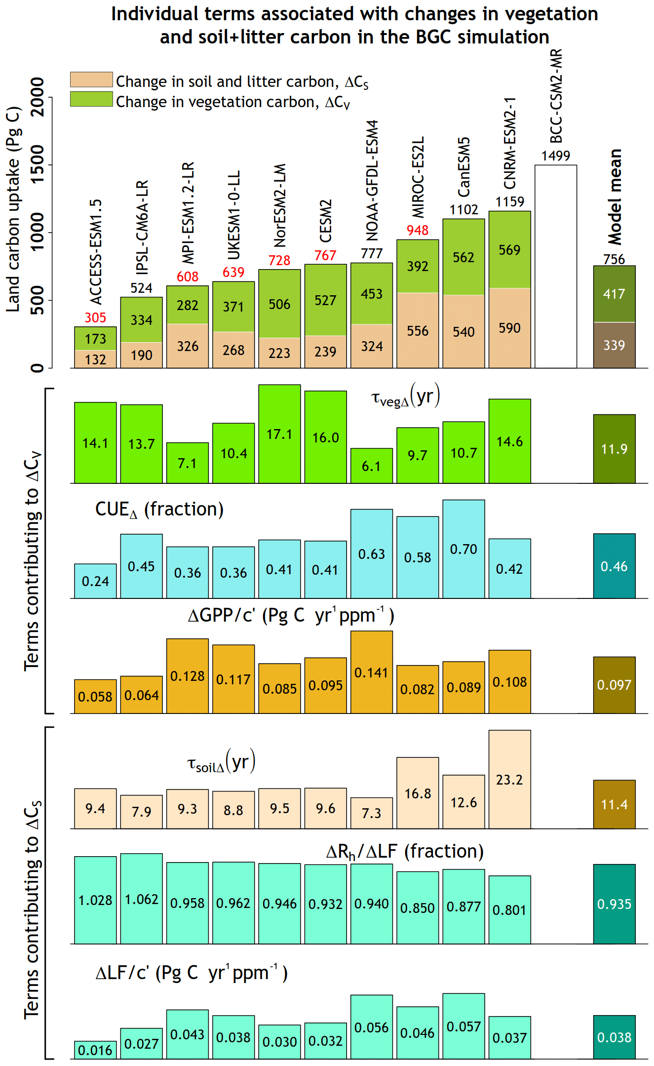
Figure 8Individual terms of Eq. (8) which contribute to changes in vegetation (ΔCV) and litter + soil (ΔCS) carbon pools. Values from the BCC-CSM2-MR model are not used in calculating the model mean.
Figure 8 shows the individual components of Eq. (8) which contribute to terms corresponding to changes in vegetation (ΔCV) and soil + litter (ΔCS) carbon pools. Figure 7a is repeated in Fig. 8 for the easy matching of individual components of Eq. (8) with their corresponding models. The model mean values of individual terms do not take into account the results from the BCC-CSM2-MR model as explained in the figure caption. In essence, the terms in Fig. 8 are emergent properties of the land models of the individual ESMs and result from their multiple interacting processes. The comparison of the individual terms of Eq. (8) provides additional insight into the reasons for differences in land models. For example, the CNRM-ESM2-1 model has the highest land carbon uptake among all models in the BGC simulation. However, this is not caused by a strong CO2 fertilization effect (the term) but rather by the relatively high τvegΔ and τsoilΔ values. The CO2 fertilization effect is strongest for the three models that simulate vegetation cover dynamically (NOAA-GFDL-ESM4, MPI-ESM1.2-LR, and UKESM1-0-LL) since the term also implicitly includes the effect of increasing vegetation cover as CO2 increases. The tree cover in the NOAA-GFDL-ESM4 model, for example, increases in the BGC simulation – particularly in dry, high-latitude regions above 50∘ N (not shown). However, these models do not simulate the largest land carbon uptake because of their lower-than-average τvegΔ and τsoilΔ values. The term is unable to capture the CO2 fertilization effect separately from increasing vegetation cover, and this illustrates the challenge in comparing models that do and do not simulate vegetation cover dynamically. The CanESM5 model exhibits higher-than-average land carbon uptake despite its near-average strength of the CO2 fertilization effect and τvegΔ and τsoilΔ values. However, its CUEΔ is the highest, and therefore a much larger fraction of GPP is converted to NPP. Although CUEΔ is not the same as CUE, we found that CUEΔ and CUE (calculated at the end of the 1pctCO2 simulation at 4×CO2) are strongly correlated with a correlation of around 0.90 (not shown). Similarly, τvegΔ is strongly correlated, with a correlation of 0.96, to τveg = CV ∕ NPP calculated at the end of the simulation. The ACCESS-ESM1.5 model exhibits the lowest land carbon uptake because of its weak CO2 fertilization effect and the lowest CUEΔ of all models. Finally, the term shows the least variability across models, which is reflective of the fact that the magnitude of the heterotrophic respiration flux is dominated by NPP inputs into the dead carbon pools (Koven et al., 2015). Several of these individual terms are strongly correlated. The and terms have a correlation of 0.77, and CUEΔ and have a correlation of 0.94, since a stronger CO2 fertilization effect also implies a larger litterfall flux per unit CO2. Surprisingly, CUEΔ and τvegΔ are negatively correlated (correlation = −0.49) across models, indicating that models which retain a higher fraction of GPP as NPP typically get rid of vegetation carbon sooner via litterfall as indicated by a faster turnover of vegetation (lower τvegΔ), thereby partially compensating for higher CUEΔ.
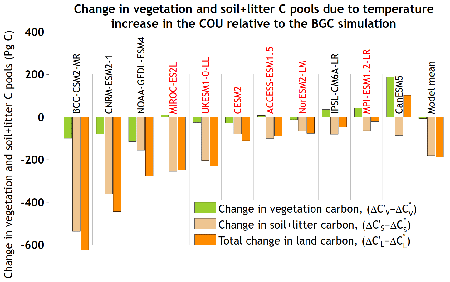
Figure 9The changes in vegetation and soil + litter carbon pools in the COU relative to the BGC simulation, as shown in Eq. (9), which contribute to the calculation of the carbon–climate feedback over land (γL) in the BGC–COU approach. The names of models which include the N cycle are shown in a red font colour.
Figure 9 investigates the reasons for varying magnitudes of the carbon–climate feedback over land (γL). In Eq. (9), γL is a function of change in land carbon (divided into vegetation and soil + litter components) in the COU relative to the BGC simulation and the temperature change in the COU simulation (T′). Over land, the higher temperatures in the COU relative to the BGC simulation affect not only both autotrophic and heterotrophic respiratory fluxes, from live and dead vegetation pools, respectively, but also gross photosynthesis rates. The primary effect of this temperature change in COU versus the BGC simulation is the loss of carbon from the soil + litter carbon pool (hence the negative sign of γL for most models; Fig. 6b and d), but changes in the vegetation carbon pool also occur. Although γL also depends on T′, Fig. 9 arranges models in order from the largest to smallest loss of land carbon in COU relative to the BGC simulation to illustrate the varying response of the models. This ordering of models changes slightly if the carbon loss (or gain in the CanESM5 model) is divided by the temperature change T′ in the COU simulation (yielding the value of γL which assumes as in Eq. 9).
As shown in Fig. 9, all models lose carbon from the soil + litter carbon pool but with widely varying magnitudes. Although typically smaller than the change in the soil + litter carbon pool, the change in the vegetation carbon pool in the COU relative to the BGC simulation is not of the same sign across models. Of the 11 participating models, 6 lose carbon in the vegetation pool in the COU relative to the BGC simulation, thereby contributing to increasing the absolute magnitude of γL, while the remaining 5 exhibit an increase in the vegetation carbon pool, thereby decreasing the absolute magnitude of γL. The largest increase in the vegetation carbon pool is seen in the CanESM5 model that more than compensates for the carbon loss from the soil + litter carbon pool, yielding a positive value of γL in contrast to other models. This case is one of the few times a positive value of γL is seen in an Earth system model. Thornton et al. (2009) reported positive γL after their first attempt to include N cycle in the CLM. Preliminary analysis of CanESM5 data shows the increase in vegetation carbon in the COU relative to the BGC simulation is caused by the increase in GPP and the resulting vegetation growth at middle to high latitudes in response to warming temperatures and increasing CO2. Interestingly, this response is not seen at 2×CO2 (see Table A1 in the Appendix), and γL is still negative for CanESM5.
Table 3Correlation between carbon–concentration (βX) and carbon–climate (γX) feedback parameters over land and ocean across comprehensive ESMs from the CMIP5 intercomparison in the A13 study and CMIP6 intercomparison in this study. For the land correlation it is also shown when CanESM5 is excluded from CMIP6 models.
The loss in land carbon in the COU relative to the BGC simulation (except for the CanESM5 model that gains carbon), indicated by the dark orange bars in Fig. 9, is strongly correlated with the carbon gain in the BGC simulation (Fig. A1e; correlation is 0.59 for all models and 0.87 when CanESM5 is excluded) but not with the absolute amount of total land carbon. Figure A3 in the Appendix shows the absolute amount of carbon in soil + litter and vegetation pools, and their change from the beginning, for the BGC simulation. The models vary widely in terms of the absolute size of the carbon pools, especially for the soil + litter pool. There are two implications of models losing more carbon in the COU relative to the BGC simulation when they take up more carbon in the BGC simulation alone. First, the transient behaviour of a model is determined primarily by its response to CO2 and temperature perturbations and not by the absolute amount of land carbon. Second, carbon–concentration (βX) and carbon–climate (γX) feedback parameters must be correlated as well. Indeed, this is not only the case over land for both CMIP5 and CMIP6 models but also true for ocean feedbacks although the correlations are somewhat weaker over the ocean. These correlations are shown in Table 3 and are negative since higher positive values of βX are correlated with higher negative values of γX, indicating that models that take up more carbon with increasing CO2 also release more carbon when they “see” the associated higher temperatures.
4.4.2 Ocean
The time-integrated air–sea flux of carbon provides the dominant contribution to the increase in global ocean carbon through changes in the DIC inventory. However, the global ocean carbon inventory is also affected by the land-to-ocean carbon flux from river runoff and the carbon burial in ocean sediments (see Table A2 in the Appendix).
Ocean carbon cycle feedbacks are defined in terms of ocean carbon inventory changes for the COU simulation and by the differences in COU relative to the BGC simulation. To fully understand the ocean carbon cycle feedbacks, it is necessary to understand the ocean carbon distributions for the preindustrial period and then analyze the carbon anomalies relative to the preindustrial period for these climate model experiments.
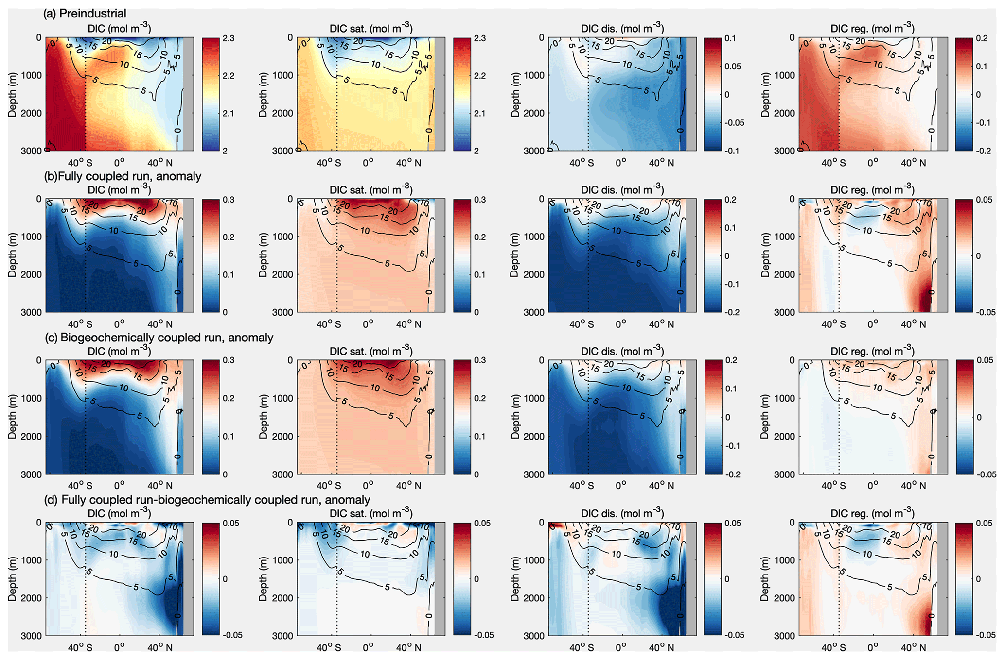
Figure 10Meridional section of the dissolved inorganic carbon, DIC (mol m−3), and constituent carbon pools in UK-ESM1-0-LL for the zonally averaged Atlantic and Southern Ocean: (a) the preindustrial absolute concentrations and (b–d) the anomalies relative to the preindustrial state at year 140 for (b) the COU configuration, (c) the BGC configuration, and (d) the COU minus the BGC configuration. The DIC is separated into saturated carbon, DICsat, the disequilibrium carbon, DICdisequilib, and the regenerated carbon, DICregenerated. The Atlantic and Southern Ocean domains are separated by a vertical black line.
Ocean carbon distribution
The ocean dissolved inorganic carbon, DIC, distribution is controlled by a combination of physical, chemical, and biological processes. For the preindustrial period, there is less DIC in the warmer waters of the upper ocean and more DIC in the colder mid-depth and bottom waters (Figs. 10a, 11a; illustrated here for UKESM1-0-LL as a representative example, and Figs. S1 to S7 show similar distributions for all the diagnosed Earth system models). The vertical extent of the low DIC follows the undulations of the thermocline, which is defined by strong vertical temperature and density gradients, and is deeper over the subtropical gyres at 30∘ N and 30∘ S and shallower in the equatorial zone and at high latitudes. The greater DIC at depth is a consequence of greater solubility in colder waters and the accumulation of DIC from the regeneration of organic matter.
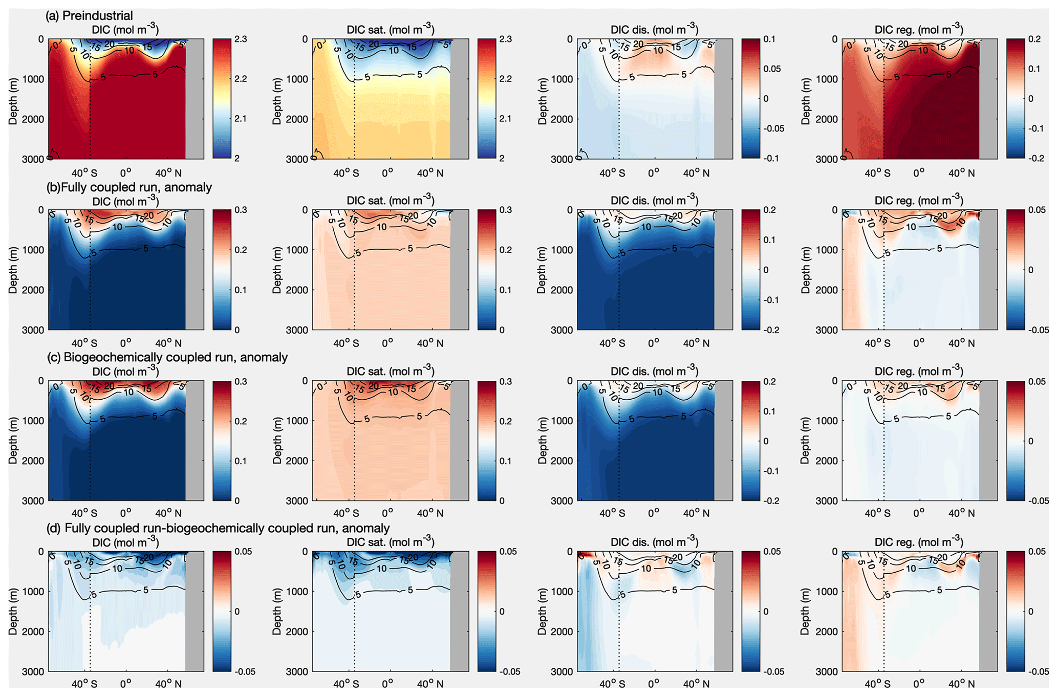
Figure 11Meridional section of the dissolved inorganic carbon, DIC (mol m−3), and constituent carbon pools in UK-ESM1-0-LL for the zonally averaged Pacific and Southern Ocean: (a) the preindustrial absolute concentrations and (b–d) the anomalies relative to the preindustrial state at year 140 for (b) the COU configuration, (c) the BGC configuration, and (d) the COU minus the BGC configuration. The DIC is separated into saturated carbon, DICsat, the disequilibrium carbon, DICdisequilib, and the regenerated carbon, DICregenerated. The Pacific and Southern Ocean domains are separated by a vertical black line.
To gain insight into how the ocean carbon distribution is controlled, the DIC is separated into three pools, DICsat, DICdisequilib, and DICregenerated, as defined earlier. The DIC distribution for both the preindustrial period and after 140 years in the 1pctCO2 simulation reveal the following key features for each of these carbon pools (Figs. 10a, b and 11a, b):
-
The saturated carbon pool provides the dominant contribution to the DIC, holding more than 2.15 mol C m−3, particularly within cooler waters below the thermocline.
-
The regenerated carbon pool enhances the carbon stored below the surface waters, typically providing an additional 0.2 mol C m−3 within the Southern Ocean and older waters spreading from the Southern Ocean into the Atlantic and below the thermocline in the Pacific.
-
The disequilibrium carbon is small close to the surface, representing waters close to an equilibrium with the atmosphere. There is sometimes a positive disequilibrium of up to 0.05 mol C m−3 in some surface waters, which is associated with upwelling transferring carbon-rich deeper waters to the surface. The disequilibrium carbon is more strongly negative below the thermocline, typically reaching −0.1 mol C m−3 in the Atlantic and −0.02 mol C m−3 in the Southern Ocean and Pacific. In the preindustrial period, the undersaturation in carbon below the thermocline is due to the subduction of cold waters at high latitudes that have not equilibrated fully with the atmosphere, which then spread by advection along density surfaces. In the model integrations reaching year 140, the carbon below the thermocline becomes further undersaturated relative to the contemporary atmosphere due to the rapid rise in [CO2].
Next we consider the anomalies in the DIC at year 140 in the COU configurations of the 1pctCO2 simulation calculated relative to the preindustrial period. The carbon anomaly, ΔDIC, in the COU configuration is positive over the upper thermocline over the Atlantic and Pacific basins, reaching +0.3 mol C m−3, coinciding with regions that are well ventilated. This gain in carbon is made up of an increase in the saturated carbon over all depths due to higher atmospheric CO2. There is a dipole in the disequilibrium anomaly (Figs. 10b, c and 11b, c); it is generally weakly positive in the upper ocean and more strongly negative in deeper waters below the thermocline reaching up to −0.2 mol C m−3. This negative disequilibrium anomaly in deeper waters is smallest in the relatively well-ventilated mid-depth waters of the North Atlantic but extends over nearly all of the more poorly ventilated mid-depth waters of the Pacific (Figs. 10b and 11b).
The regenerated carbon anomaly is relatively small in magnitude, reaching less than 0.05 mol C m−3, and varies regionally, enhanced within much of the North Atlantic and the thermocline of the Pacific but with little change in the deep waters of the Pacific (Figs. 10b and 11b). The increase in regenerated carbon is due to a weakening of ocean overturning leading to an increase in residence time and an associated accumulation of DIC from the regeneration of biologically cycled carbon (Bernardello et al., 2014; Schwinger et al., 2014). The regenerated carbon signal does not change in the mid-depths and deep Pacific as 140 years is too short an integration timescale for any effect to be detected.
To diagnose the carbon cycle feedback parameters, the ocean carbon response needs to be considered for the BGC configuration where there is only limited warming from the increase in atmospheric CO2 and therefore limited change in climate and ocean circulation. The resulting DIC anomalies are generally very similar to those for the COU configuration (Figs. 10b, c and 11b, c), which is to be expected as the dominant effect for the ocean carbon response is the enhanced ocean uptake of carbon in response to the increase in [CO2]. There is a weakening in ventilation in the COU configuration due to the additional radiative forcing. In comparison, in the BGC configuration, there is no change in the circulation as there is no radiative warming effect, so there is slightly more carbon uptake in the northern North Atlantic, such as revealed at around 50∘ N, compared with the COU configuration. For the BGC configuration, the saturated carbon pool is slightly greater at depth due to the water masses being cooler than in the COU configuration, the disequilibrium anomaly shows a less negative anomaly in the northern North Atlantic because there is little or no change in ventilation, and there are only slight differences in the regenerated pool.
The climate response to rising [CO2] is now considered in terms of the difference in the COU and BGC configurations, which includes the combined effects of warming and circulation changes (Figs. 10d and 11d). The surface warming drives a decrease in solubility, an increase in stratification, and a reduction in ventilation, which leads to an overall decrease in carbon uptake over the Southern Ocean and Pacific basins and much of the Atlantic basin. There is a decrease in the saturated carbon pool associated with the warming acting to inhibit carbon uptake. The regenerated carbon anomaly is enhanced in the deep northern North Atlantic and in the Southern Ocean. The regenerated carbon anomaly for this climate response is very similar to that for the COU configuration, suggesting that the regenerated carbon anomaly is mainly due to circulation changes: the gain in the regenerated carbon anomaly is consistent with the expected longer residence time from weaker overturning and ventilation. There is a more negative disequilibrium anomaly in the deep waters of the North Atlantic, which is a consequence of weaker ventilation.
To gain more insight into the disequilibrium response, the ocean DIC response is also considered for the radiatively coupled integration (RAD), where the ocean biogeochemistry does not see the increase in [CO2]. The warming in the RAD simulation leads to a weakening in the overturning, which enhances the residence time in the surface waters and so generally decreases the magnitude of the disequilibrium anomaly in the North Atlantic (Fig. S8), making the disequilibrium less negative relative to the preindustrial period and so forming a positive disequilibrium anomaly at year 140. In comparison the COU–BGC approach captures the effect of the warming under rising [CO2], leading to the disequilibrium anomaly instead becoming more negative at depth, since the weakening in the ventilation leads to more of the anthropogenic carbon remaining at the surface rather than being transferred into the deeper ocean (Schwinger et al., 2014).
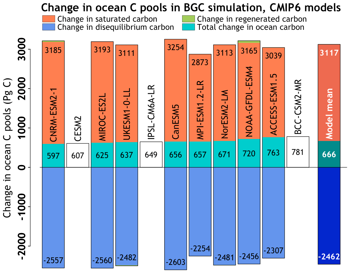
Figure 12Carbon uptake over the ocean in the biogeochemically coupled simulation, used to calculate the ocean carbon–concentration feedback and its partitioning into saturated, disequilibrium, and regenerated carbon pools across the participating CMIP6 models (left) using Eq. (12). No partitioning is shown for models for which 3D ocean fields were not available, and the results of these models are not used in calculating the model mean values (right). The sum of the partitions does not exactly match the total ocean uptake diagnosed from the air–sea fluxes due to land–ocean interactions involving storage in sediments and river inputs.
Changes in ocean carbon pools for diagnosing feedback parameters
The ocean carbon–concentration feedback parameter, βO, is diagnosed from the changes in the ocean carbon inventories for the BGC configuration, which does not include radiative warming due to increasing [CO2] (Eq. 13). There is a consistent increase in ocean carbon storage across all models with a model mean value of around 670 PgC (Fig. 12, turquoise bars). This increase in ocean carbon storage is made up of an increase in the saturated carbon inventory, ΔCsat, by about 3100 PgC from the increase in [CO2] (Fig. 12, red bars). This increase is partly offset by a more negative disequilibrium carbon, ΔCdisequilib, of typically −2500 PgC (Fig. 12, blue bars), representing how the ocean carbon uptake cannot keep up with the rate of [CO2] increase. There is relatively little change in the regenerated carbon inventory, ΔCregenerated. The resulting βO is positive and mainly explained by the chemical response involving the rise in ocean saturation with no significant biological changes, although the physical uptake of carbon within the ocean is unable to keep pace with the rise in [CO2].
The ocean carbon–climate feedback parameter, γO, is diagnosed from the difference between the COU model configuration and the BGC configuration and so includes the effect of an increasing surface warming under rising [CO2] (Eq. 14). There is a broadly consistent response across models, with a model mean decrease in carbon inventory of around 80 PgC due to the additional warming in the COU configuration relative to the BGC configuration (Fig. 13, turquoise bars). The effect of this additional warming and the associated climate change leads to a decrease in both the saturated carbon and disequilibrium carbon of typically −60 and −70 PgC (Fig. 13, orange and blue bars), representing the decrease in solubility and decreased ocean ventilation. There is an increase in the regenerated carbon of typically 50 PgC (Fig. 13, green bars), which is due to a weaker circulation leading to a longer residence time of thermocline and deep waters, so there is more time for the accumulation of regenerated carbon below the mixed layer. The resulting γO is negative, indicating that the ocean takes up less carbon in response to the combination of surface warming and a weakening in ocean ventilation. This response involves a combination of chemical, physical, and biological changes where the warming reduces the solubility of the carbon in the ocean and a weakening in the circulation decreases the disequilibrium pool but lengthens the residence time and so increases the regenerated pool.
Overall, the ocean carbon inventory increases in the BGC configuration by 666 ± 53 PgC (model mean ± standard deviation) and decreases in COU relative to BGC by −80 ± 15 PgC. The resulting βO is very similar across all the models (0.78 ± 0.06 PgC ppm−1), reflecting not only the strong control of carbonate chemistry by rising atmospheric CO2 (Katavouta et al., 2018) but also the use of similar carbonate chemistry schemes and bulk parameterizations of air–sea CO2 fluxes across marine biogeochemical models (Séférian et al., 2020). The dominant contributions are composed of a positive contribution from the saturated carbon (3.66 ± 0.16 PgC ppm−1) and a negative contribution from the disequilibrium carbon (−2.98 ± 0.16 PgC ppm−1; see Table A3 in the Appendix); these intermodel differences are relatively small with ratios of the standard deviation to model mean of only 0.05 and 0.06, respectively. The regenerated contribution is over 2 orders of magnitude smaller than the sum of the saturated and disequilibrium contributions and so may be neglected for evaluating βO.

Figure 13Change in saturated, disequilibrium, and regenerated carbon pools in the fully coupled minus the biogeochemical simulation using Eq. (14), which contributes to the calculation of the carbon–climate feedback over the ocean. The sum of the partitions does not exactly match the total ocean uptake diagnosed from the air–sea fluxes due to land–ocean interactions involving storage in sediments and river inputs.
The values of γO differ more strongly across the models (−16.95 ± 5.62 PgC ∘C−1) and arise from differences in the extent of the surface warming and the dynamical changes in the ocean circulation and resulting changes in ventilation, residence time, and biological regeneration (Table A3). The contributions to γO include negative contributions from the saturated (−12.78 ± 2.50 PgC ∘C−1) and disequilibrium (−16.36 ± 5.31 PgC ∘C−1) components, which are partly opposed by a positive contribution from the regenerated component (12.25 ± 8.53 PgC ∘C−1). The largest intermodel differences are in the regenerated and disequilibrium responses and a relatively small spread in the saturated response, with the ratios of the standard deviation to the model mean being 0.70, 0.33, and 0.20, respectively (Table A3).
4.5 Transient climate response (TCR) and transient climate response to cumulative emissions (TCRE)
The idealized 1pctCO2 simulation is also routinely used for calculating two other climate metrics. The first is the transient climate response (TCR), which is defined as the temperature change relative to the preindustrial state at the time of CO2 doubling (), which occurs at 70 years after the start of the simulation. The second is the transient climate response to cumulative carbon emissions (TCRE), which is defined as the ratio of the TCR to cumulative fossil fuel emissions also at the time of CO2 doubling (; Matthews et al., 2009), typically expressed in units of degrees Celsius per exagram of carbon (EgC−1; 1 EgC = 1000 PgC).
It has been shown that the TCRE is approximately constant over a wide range of cumulative emissions and emission pathways (MacDougall, 2016). Although non-CO2 greenhouse gases and other climate forcings (e.g. aerosols and land use change) also affect the realized warming, the TCRE is considered to be a straightforward measure of peak warming caused by anthropogenic CO2 emissions. The TCRE metric has gained significant policy relevance (Frame et al., 2014; IPCC, 2014; Millar et al., 2016), and it is a central component of frameworks used to calculate the remaining allowable carbon emissions to reach a specified temperature change target above the preindustrial level (Millar et al., 2017; Rogelj et al., 2018, 2019).
Table 4Transient climate response (TCR; ), diagnosed cumulative emissions at 2×CO2 (), and transient climate response to cumulative emissions (TCRE) for the 11 CMIP6 models considered in this study.
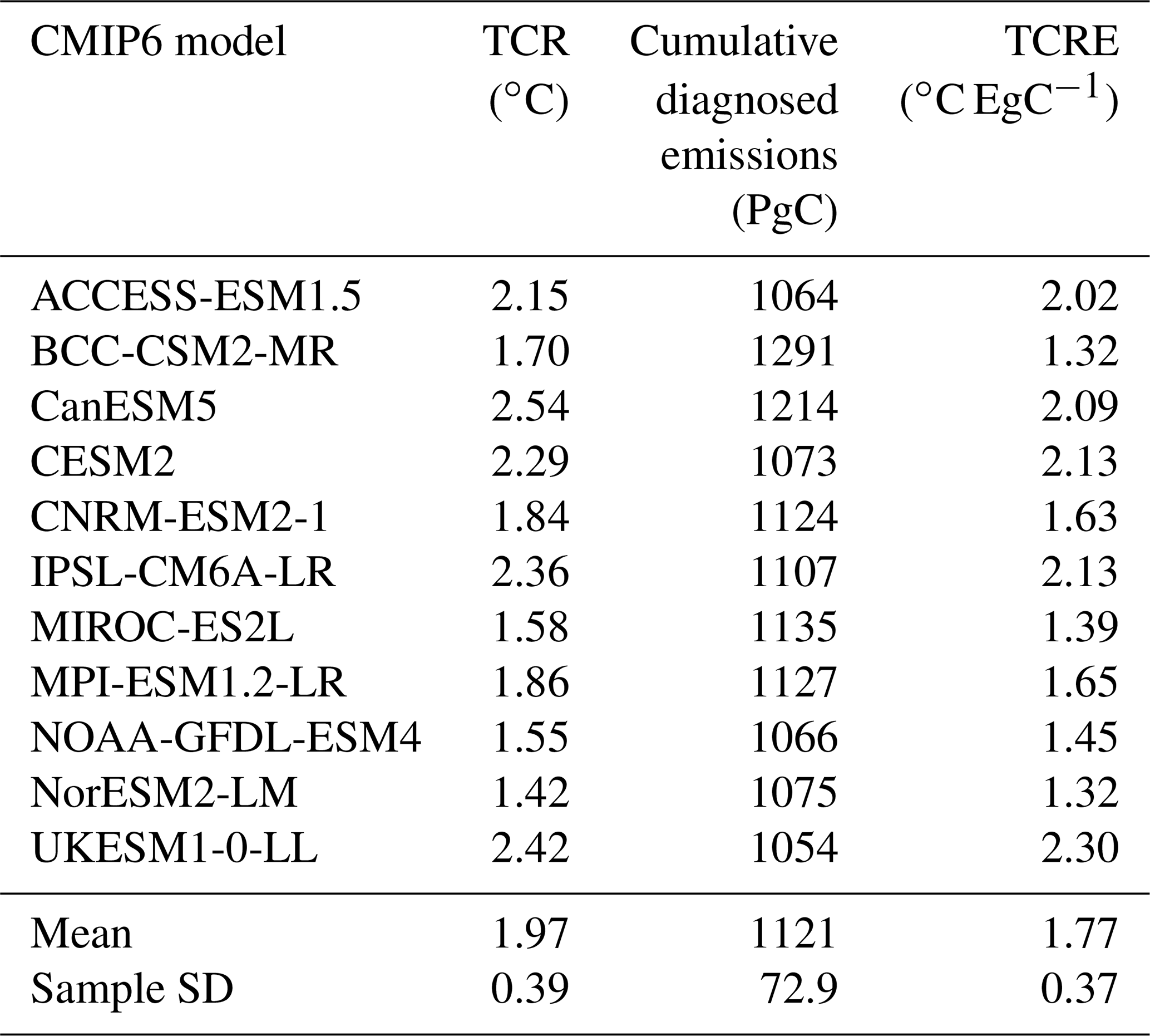
Table 4 lists the TCR, , and TCRE from the 11 CMIP6 models considered in this study. We calculate the TCR, following the standard approach, as the average temperature of 20 years (years 60–79) centered on the year when CO2 doubles (year 70). The mean ± standard deviation for the TCR, , and the TCRE from the 11 CMIP6 models considered here is 1.97 ± 0.39 ∘C, 1121 ± 73 PgC, and 1.77 ± 0.37 ∘C EgC−1, respectively. For 15 CMIP5 models, Gillett et al. (2013) calculated the TCRE to be 1.63 ± 0.48 ∘C EgC−1 and a 5 %–95 % range for its observationally constrained value as 0.7–2.0 ∘C EgC−1. The CMIP5 and CMIP6 mean values quoted are not statistically different given the small sample size of available models, some of which duplicate processes or components.
The uncertainties in the TCRE stem from uncertainties in both the TCR and which is directly affected by land and ocean carbon uptake. A large fraction of uncertainty in comes from the diverse response of land carbon cycle models. Inclusion of the N cycle helps to reduce this uncertainty in terms of the spread across the land models (both the strength of their feedback parameters and diagnosed cumulative emissions). Cumulative diagnosed emissions for models with the land N cycle total 1088 ± 34 PgC compared to 1160 ± 91 PgC for models without the N cycle (from Table 4). For the results reported here from 11 CMIP6 models, however, the uncertainty in the TCR (mean ± standard deviation = 1.97 ± 0.39 ∘C), as indicated by standard deviation normalized by the mean, is 3 times as big as the uncertainty in (1121 ± 73 PgC). As a result, the TCR contributes about 90 % of the total variance in the calculated TCRE value (1.77 ± 0.37 ∘C EgC−1; see Sect. A6 in the Appendix).
The TCRE may also be expressed in terms of a product of a thermal contribution from the dependence of surface warming on radiative forcing and a carbon contribution from the dependence of radiative forcing on cumulative carbon emissions (Williams et al., 2016; Katavouta et al., 2018), as
where is the change in radiative forcing relative to the preindustrial period. For a suite of 10 CMIP5 models, Williams et al. (2017) show that the intermodel spread in the TCRE calculated from the 1pctCO2 experiment has a larger contribution from the intermodel differences in the thermal contribution, , due to climate feedback and ocean heat uptake over the first few decades, but the intermodel differences in the carbon contribution, , due to land and ocean carbon uptake become of comparable importance after 80 years.
Thus we conclude, as shown by Jones and Friedlingstein (2020), that the contributions to TCRE uncertainty have changed since CMIP5 from being of similar magnitudes due to carbon feedbacks and climate feedbacks to now being dominated by climate feedbacks. The reduction in the spread of land carbon model feedbacks which we are beginning to see in CMIP6 has led to a reduction in the spread of the TCRE implying that a large fraction of uncertainty in the TCRE is now contributed to by physical climate system processes that determine the TCR. More CMIP6 models include a complete treatment of important processes – notably the terrestrial nitrogen cycle – that determine the airborne fraction and hence . Reducing the uncertainty in land and ocean carbon uptake across models remains a priority and will contribute to further reducing the uncertainty in the estimates of the TCRE on centennial timescales.
Model intercomparison projects offer several benefits including the calculation of the model mean response, the quantification of the uncertainty based on the spread across models, and showing how this uncertainty changes over time. The carbon feedback analysis presented here based on the C4MIP protocol of experiments (Jones et al., 2016) allows us to investigate how feedback strengths have evolved since CMIP5 and also to attempt to understand the reasons behind the spread in models.
The carbon uptake over land and ocean, in response to increasing atmospheric CO2 concentration, is well known to be dominated by the positive contribution from the carbon–concentration feedback (Gregory et al., 2009; Arora et al., 2013). The strength of this feedback is of comparable magnitudes over land (mean ± standard deviation = 0.97 ± 0.40 PgC ppm−1) and ocean (0.79 ± 0.07 PgC ppm−1) although the feedback is much more uncertain over land as indicated by the standard deviation across the 11 models considered here. This dominant positive contribution from the carbon–concentration feedback is, however, opposed by the weaker negative carbon–climate feedback that is associated with the climate change that results due to increasing atmospheric CO2. The absolute magnitude of this weaker negative feedback is about 3 times larger and an order of magnitude more uncertain over land (−45.1 ± 50.6 PgC ∘C−1) than over ocean (−17.2 ± 5.0 PgC ∘C−1). Model estimates of the ocean carbon–concentration feedback are consistent with each other, reflecting the strong control of how carbonate chemistry alters with rising atmospheric CO2. There is a relatively wider range in the model estimates of the ocean carbon–climate feedback, particularly in terms of how changes in ocean circulation alter the disequilibrium and regeneration terms. Over land, however, since the carbon–concentration and carbon–climate feedbacks are determined entirely by biological process, which are much less understood, the resulting uncertainty is much higher across the land models than across the ocean models. This uncertainty in the strength of carbon–concentration and carbon–climate feedbacks over land is well known (Friedlingstein et al., 2006; Arora et al., 2013). The inclusion of the N cycle results in lower absolute strength of the feedback parameters over land. In addition, the land models that include a representation of the N cycle exhibit a reduced spread in their feedback parameters, despite the additional complexity, compared to when all models are considered. This suggests that if all models were to include the N limitation of photosynthesis, the spread across them will potentially reduce.
The additional analyses that we have performed provide insight into the reasons for the diverse responses among models, especially for land models. Over land, the diverse response of models is found to be primarily due to the wide range of the strength of the CO2 fertilization effect, the fraction of GPP that is converted to NPP, and the residence times of carbon in the live (vegetation) and dead (litter plus soil) carbon pools across models. There is more consistency in the response of the ocean models, although intermodel differences arise from differences in the ventilation and residence time, altering the ocean disequilibrium and regenerated carbon.
In regard to the TCRE, while its uncertainty is dominated by physical processes affecting the thermal response involving climate feedbacks and heat uptake on decadal timescales, a reduction in the uncertainty in land and ocean carbon uptake across models will reduce the uncertainty in the TCRE on centennial timescales.
Finally, the decision to use fully and biogeochemically coupled configurations of the 1pctCO2 experiment as the standard simulations from which to diagnose carbon cycle and climate system feedbacks should provide consistency and continuity for future versions of Earth system models that can be compared against their predecessors.
The rate of change in carbon in the combined atmosphere–land–ocean system is written as
where the global carbon pool CG = CA + CL + CO is the sum of carbon in the atmosphere, land, and ocean components (PgC) and E is the rate of anthropogenic CO2 emissions (PgC yr−1) into the atmosphere. The equations for the atmosphere, land, and ocean are
where is the fluxes between the atmosphere and the underlying land and ocean, taken to be positive into the components. The fluxes F are expressed as functions of surface temperature T and the surface atmospheric CO2 concentration c. Here and subsequently, uppercase C denotes carbon pools and lowercase c denotes atmospheric CO2 concentration.

Figure A1Individual model values from CMIP6 models for globally averaged surface temperature change (a–c), cumulative atmosphere–land CO2 flux (d–f), and cumulative atmosphere–ocean CO2 flux (g–h) from the fully, biogeochemically, and radiatively coupled versions of the 1pctCO2 experiment.
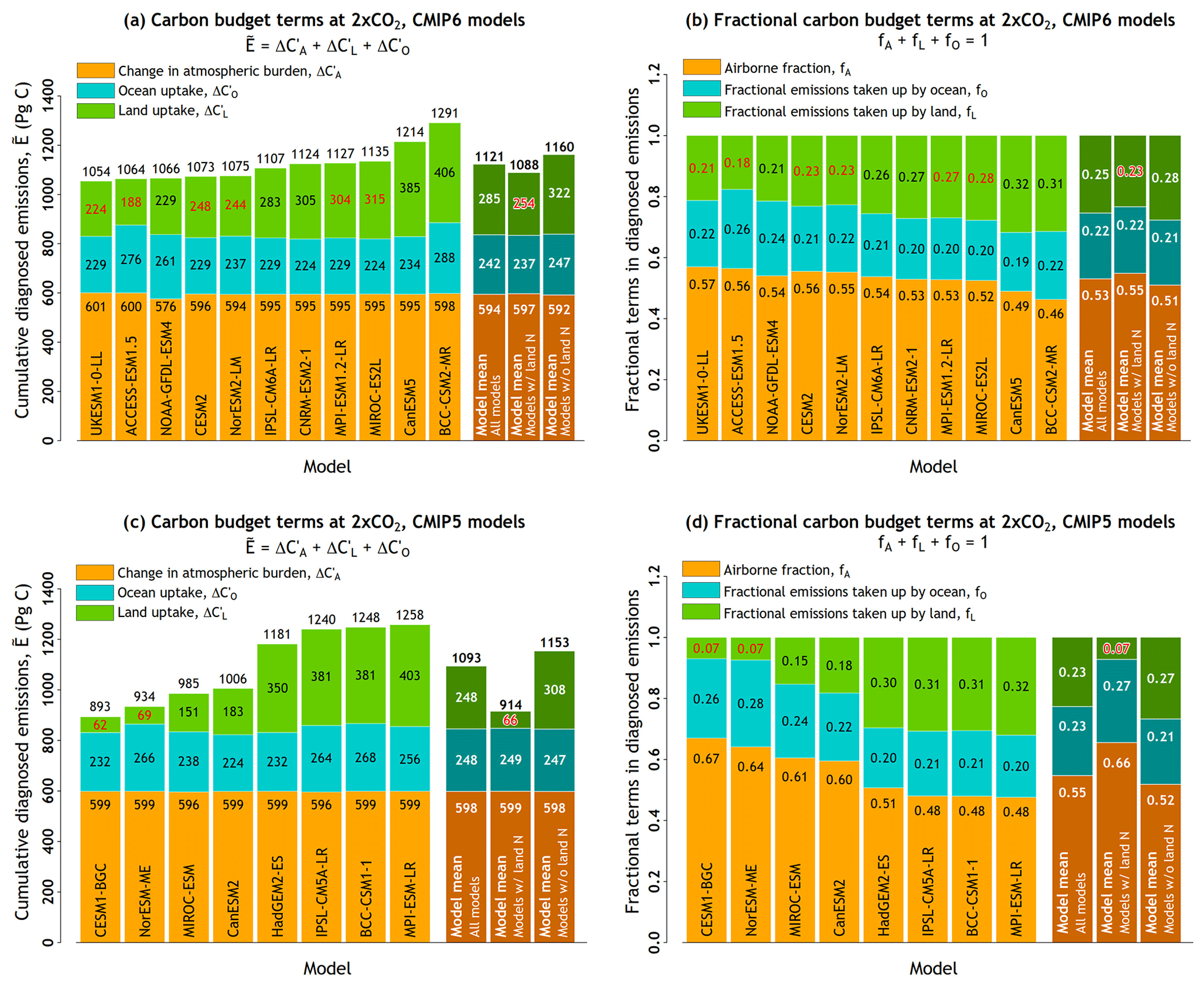
Figure A2Components of the carbon budget terms in cumulative emissions from the 11 participating CMIP6 models based on Eq. (A6) in (a) and Eq. (A7) in (b), using results from the fully coupled 1 % yr−1 increasing CO2 simulation at 2×CO2 (year 70) in contrast to Fig. 4 which showed these results at 4×CO2. The models are arranged in ascending order based on their cumulative emissions values. Results from participating CMIP5 models in the A13 study are shown in (c, d). In addition, ESMs whose land component includes a representation of the N cycle are identified by a red font colour for cumulative land carbon uptake (a, c) and fractional emissions taken up by land (b, d). The model mean is shown not only for all models but also separately for models whose land components include or do not include a representation of the N cycle.
In the fully, biogeochemically, and radiatively coupled versions of the 1pctCO2 experiments analyzed here, the rate of change in atmospheric carbon dCA / dt is specified in Eqs. (A1) and (A2). The uptake or release of CO2 by the underlying land and ocean yields an effective emission E which serves to maintain the budget.
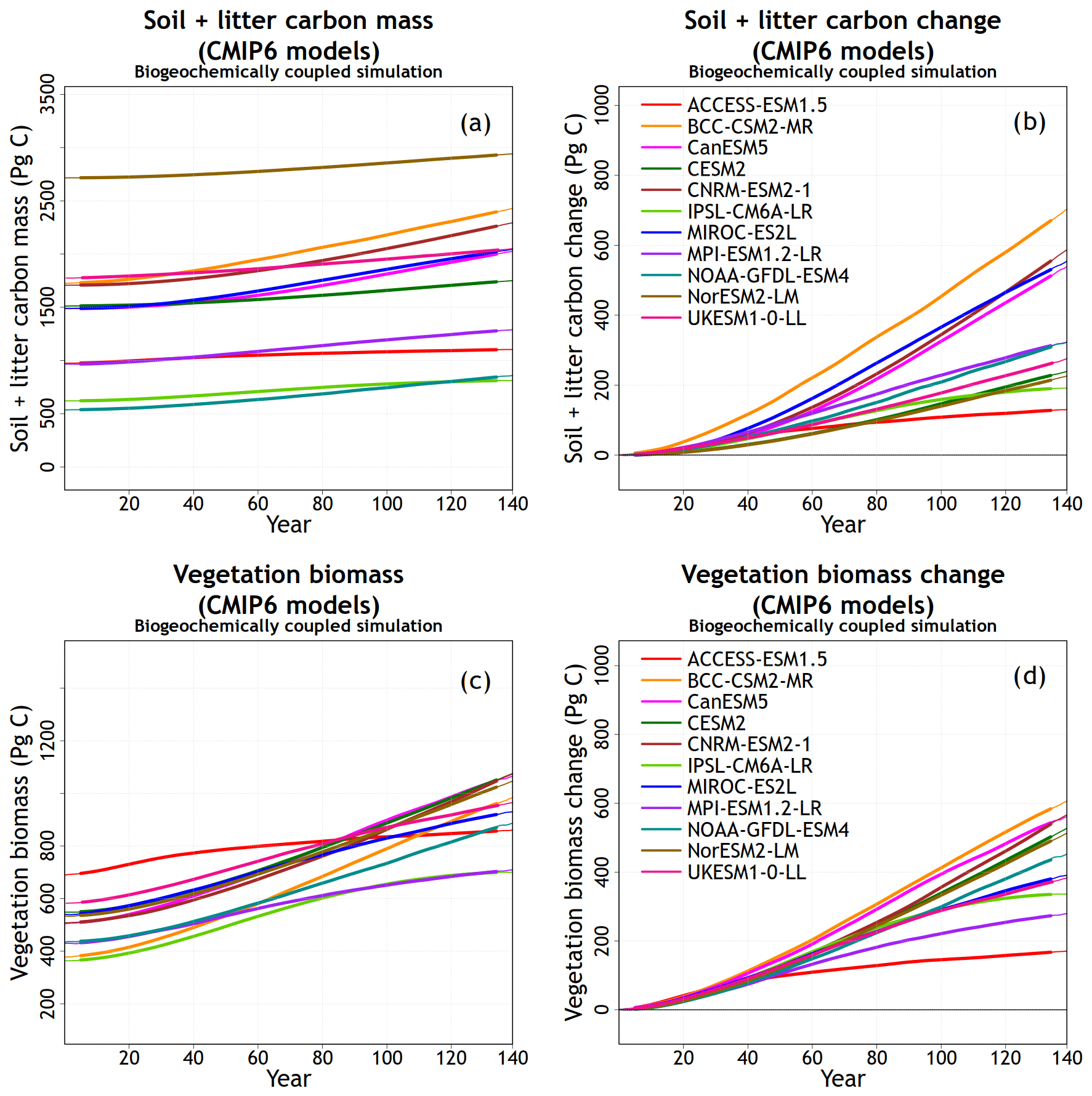
Figure A3Absolute amounts and the change from the beginning of the BGC simulation for carbon in soil + litter (a, b) and vegetation (c, d) pools.
The changes in atmosphere carbon budgets, from the preindustrial control simulation, in the differently coupled simulations are represented as
which serve to define the instantaneous carbon–concentration (BA) and carbon–climate (ΓA) feedback parameters and assume linearization of the globally integrated surface–atmosphere CO2 flux in terms of global mean temperature and concentration change. In Eq. (A3), F+, F∗, and F′ are the flux changes and T+, T∗, and T′ the temperature changes in the radiatively, biogeochemically, and fully coupled simulations, and E+, E∗, and E are the resulting implicit emissions. c′ is the specified CO2 concentration change above its preindustrial level in the 1pctCO2 simulations. In the biogeochemically coupled simulation there is no radiative forcing due to increasing CO2, so T∗ is small, although not zero, and exhibits a distinct spatial pattern. The assumption made in Eq. (A3) is that the feedback parameters are the same in the three cases.
Carbon budget changes for the land component parallel to Eq. (A3) but without the emissions terms as
and similarly for the ocean component. Since it follows that and . There are no terms involving c′ in the radiatively coupled simulation (Eqs. A3a and A4a) since the preindustrial value of atmospheric CO2 concentration is prescribed for the biogeochemistry components, so and does not affect the flux.
The instantaneous feedback parameters (BL and ΓL) differ from those in the integrated flux approach of Friedlingstein et al. (2006), who express time-integrated flux changes (i.e. change in pool or reservoir sizes) as functions of temperature and CO2 concentration changes with
and similarly for the ocean component, with the assumption that the term includes changes in the carbon amount of ocean sediment as well.
The units of instantaneous and integrated flux-based parameters are different (Γ–PgC yr−1 ∘C−1, B– PgC yr−1 ppm−1 and γ–PgC ∘C−1, β–PgC ppm−1). Arora et al. (2013) show how the instantaneous and integrated flux-based feedback parameters are related to each other
Integrating Eqs. (A1) and (A2) from initial time to t gives
Here is the change in atmospheric carbon burden (the factor 2.12 converts atmospheric CO2 concentration from parts per million to atmospheric burden in petagrams of carbon) and is the cumulative flux equal to the change in the land or ocean carbon pool for the fully coupled simulation. The terms in Eq. (A6) indicate the contribution of changes in atmosphere, land, and ocean carbon pools to cumulative emissions . Finally, division by the cumulative emissions term in Eq. (A6) gives all the terms in a fractional form as
where fA is the airborne fraction of cumulative emissions and fL and fO are fractional emissions taken up by the land and ocean. These components are evaluated at the time of CO2 quadrupling.
A1 Reasons for nonlinearity in the ocean C cycle response in the CNRM-ESM2-1 model
In Fig. 6 the value of γO changes sign for the CNRM-ESM2-1 model from positive when calculated using the RAD–BGC or RAD–COU approaches to negative when calculated using the BGC–COU approach. This nonlinear behaviour for a previous version of the CNRM model was documented in Schwinger et al. (2014) and is caused by the large increase in regenerated DIC in the RAD simulation, similar to the increase in the COU relative to the BGC simulation, as shown in Fig. 13 for the CNRM-ESM2-1 model. This nonlinear behaviour is stronger in CNRM-ESM2-1 compared to CNRM-ESM1, its previous version (Séférian et al., 2016), most likely due to a new parameterization for N fixation which increases ocean NPP and a revised parameterization for organic matter remineralization (in PISCESv2-gas). A contribution to a positive γO is also made by declining sea ice in the RAD simulation which leads to changes in the sign of the air–sea carbon exchange in the Southern Ocean. The vertical profile of dissolved inorganic carbon in the Southern Ocean in BGC and COU simulations (with rising [CO2]) is different from that in the RAD simulation (for the preindustrial [CO2]), and this leads to additional nonlinearities.
A2 Additional figures and discussion
Figure A1 shows results from individual CMIP6 models for which model means and ranges were shown in Figs. 1, 2, and 3 and allows for the identification of models which behave differently compared to the majority of models. In Fig. A1a and c, CanESM5 shows the largest temperature increase and NorESM2-LM and MIROC-ES2L the smallest in response to increase in [CO2] for the COU and RAD simulations, respectively. For cumulative atmosphere–land CO2 flux in the COU simulation (panel d), CanESM5 simulates the largest land carbon uptake and ACCESS-ESM1.5 the smallest. This is not the case for the BGC simulation (panel e) where land carbon uptakes from BCC-CSM2-MR and CNRM-ESM2.1 are the largest among all models, while land carbon uptake from ACCESS-ESM1.5 is the lowest. Finally, in the RAD simulation (panel f) the loss of carbon from land in response to increasing temperatures is lowest in MPI-ESM1.2-LR and largest in BCC-CSM2-MR. Over the ocean, while most models behave very similarly, the carbon uptakes in BCC-CSM2-MR, ACCESS-ESM1.5, and NOAA-GFDL-ESM4 are larger than in most models in the COU and BGC simulations. In the RAD simulation, almost all models simulate a loss of carbon from the ocean, but CNRM-ESM2.1 shows a small uptake.
A3 Additional tables
Table A1Values of carbon–concentration and carbon–climate feedback parameters for land and ocean calculated using the BGC–COU approach (using results from the BGC and COU simulations) and the linear transient climate sensitivity to CO2, from CMIP6 and CMIP5 models at 4×CO2 (i.e. at the end of the 1pctCO2 simulation) and 2×CO2.
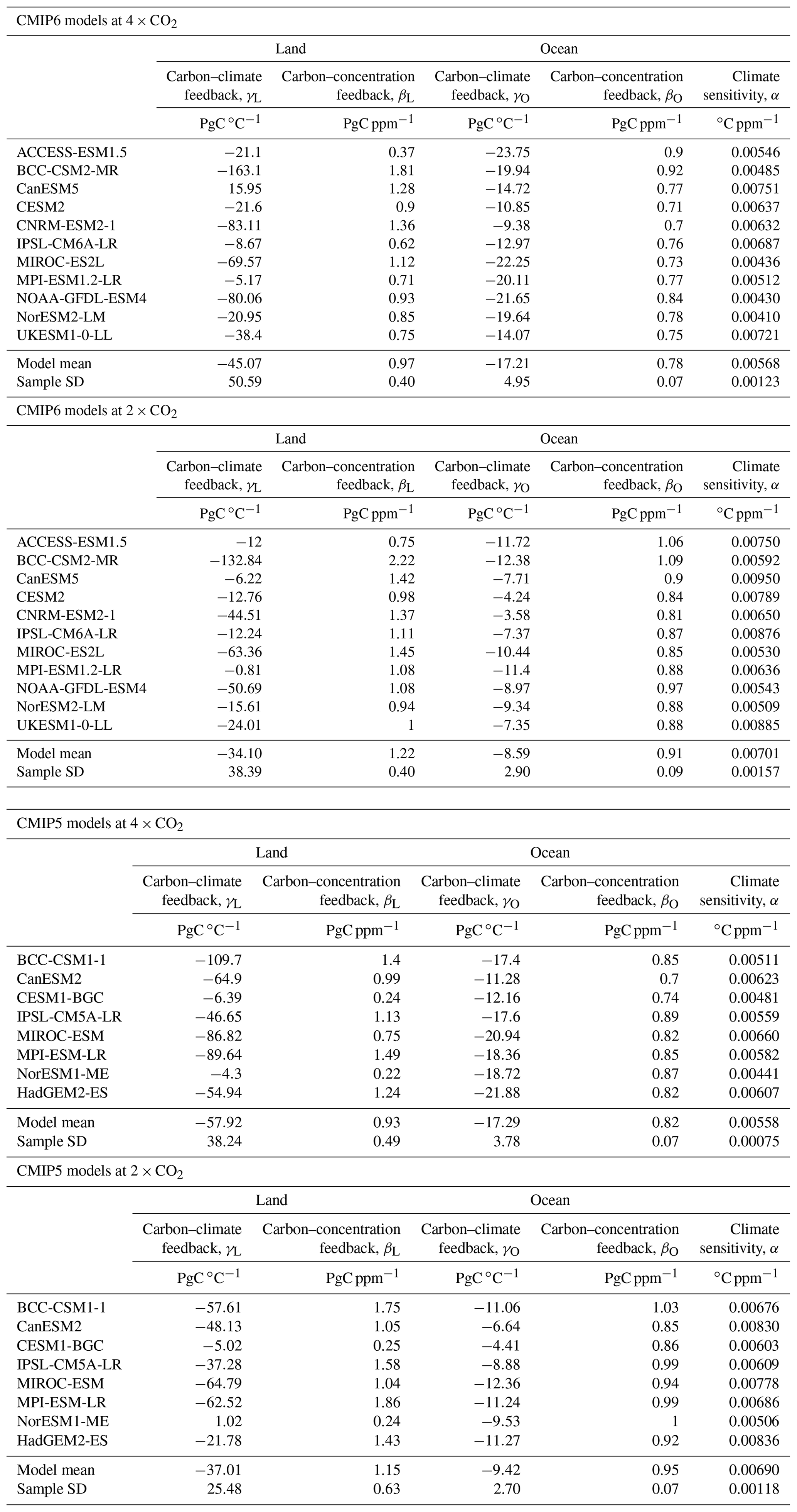
A4 Model descriptions
A4.1 Commonwealth Scientific and Industrial Research Organisation (CSIRO) ACCESS-ESM1.5
The Australian Community Climate and Earth System Simulator ACCESS-ESM1.5 (Ziehn et al., 2020) is comprised of a number of component models. The atmospheric model is the UK Met Office Unified Model version 7.3 (Martin et al., 2010, 2011) with their land surface model replaced with the Community Atmosphere Biosphere Land Exchange (CABLE) model (Kowalczyk et al., 2013). The ocean component is the NOAA GFDL Modular Ocean Model (MOM) version 5 (Griffies, 2014) with the same configuration as the ocean model component of ACCESS1.0 and ACCESS1.3 (Bi et al., 2013). Sea ice is simulated using the LANL CICE4.1 model (Hunke and Lipscomb, 2010). Coupling of the ocean and sea ice to the atmosphere is through the OASIS-MCT coupler (Valcke, 2013). The physical climate model configuration used here is very similar to the version (ACCESS1.3) that contributed to the Coupled Model Intercomparison Project Phase 5 (CMIP5; Bi et al., 2013). The carbon cycle is included in ACCESS through the CABLE land surface model and its biogeochemistry module, CASA-CNP (Wang et al., 2010), and through the World Ocean Model of Biogeochemistry and Trophic-dynamics (WOMBAT; Oke et al., 2013).
The WOMBAT model is based on an NPZD (nutrient, phytoplankton, zooplankton, and detritus) model with the additions of bioavailable iron limitation, dissolved inorganic carbon, calcium carbonate, alkalinity, and oxygen. Productivity drives uptake and formation of carbon and oxygen that are exchanged with the atmosphere. The sinking and remineralization of detritus carries biogeochemical tracers to the deep ocean. Iron is supplied by dust deposition, continental shelves, and background ocean values.
Table A2Estimate of the change in the ocean carbon inventory (PgC) expected from a time integral of the global air–sea carbon flux into the ocean versus the volume integral of the change in the dissolved inorganic carbon, together with the small residual. The time integral of the air–sea carbon flux provides the dominant contribution to the change in the ocean carbon inventory, although there is a small mismatch due to the land-to-ocean carbon flux from river runoff and the ocean-to-land carbon flux from carbon burial in ocean sediments.

The Australian community model CABLE simulates the fluxes of momentum, heat, water, and carbon at the surface. The biogeochemistry module CASA-CNP simulates the flow of carbon and nutrients such as nitrogen and phosphorus between three plant biomass pools (leaf, wood, root), three litter pools (metabolic, structural, coarse woody debris), and three organic soil pools (microbial, slow, passive), plus one inorganic soil mineral nitrogen pool and three phosphorus soil pools.
In the CABLE configuration applied here the land surface is represented by 10 vegetation and 3 nonvegetation land cover types. CABLE calculates gross primary production (GPP) and leaf respiration at every time step using a two-leaf canopy scheme (Wang and Leuning, 1998) as a function of the leaf area index (LAI). This set-up uses a simulated (prognostic) LAI based on the size of the leaf carbon pool and the specific leaf area. Daily mean GPP and leaf respiration values are then passed onto CASA-CNP to calculate daily respiration fluxes and the flow of carbon and nutrients between the pools. Similar to the previous version, ACCESS-ESM1 (Law et al., 2017; Ziehn et al., 2017), the model is run with nitrogen and phosphorus limitation enabled.
A4.2 Beijing Climate Center (BCC) Climate System Model version 2 with medium resolution (BCC-CSM2-MR)
BCC-CSM2-MR (Wu et al., 2019) is the second generation of the BCC model with medium resolution that was released to run CMIP6 simulations. It is a fully coupled global climate model and updated from its previous version of BCC-CSM1.1 used for CMIP5 (Wu et al., 2013). The atmospheric component of BCC-CSM2-MR is the BCC Atmospheric General Circulation Model version 3 (BCC-AGCM3-MR; Wu et al., 2019). The land component is the BCC Atmosphere and Vegetation Interaction Model version 2.0 (BCC-AVIM2; Li et al., 2019) with the terrestrial carbon cycle. The oceanic component is the Modular Ocean Model version 4 with 40 levels (hereafter MOM4-L40). The sea ice component is the NOAA GFDL Sea Ice Simulator (SIS). These components are physically coupled through fluxes of momentum, energy, water, and carbon at their interfaces. The coupling was realized with the flux coupler version 5 developed by the National Center for Atmosphere Research (NCAR).
Table A3Carbon cycle feedback parameters for the ocean, βO and γO, diagnosed from the air–sea carbon fluxes and separately diagnosed for the ocean carbon inventory and its separate ocean saturated, disequilibrium, and regenerated DIC pools for the subset of eight CMIP6 models for which 3D ocean data were available; their sum does not exactly match the diagnostics from the air–sea fluxes due to land–ocean interactions involving storage in sediments and river inputs.
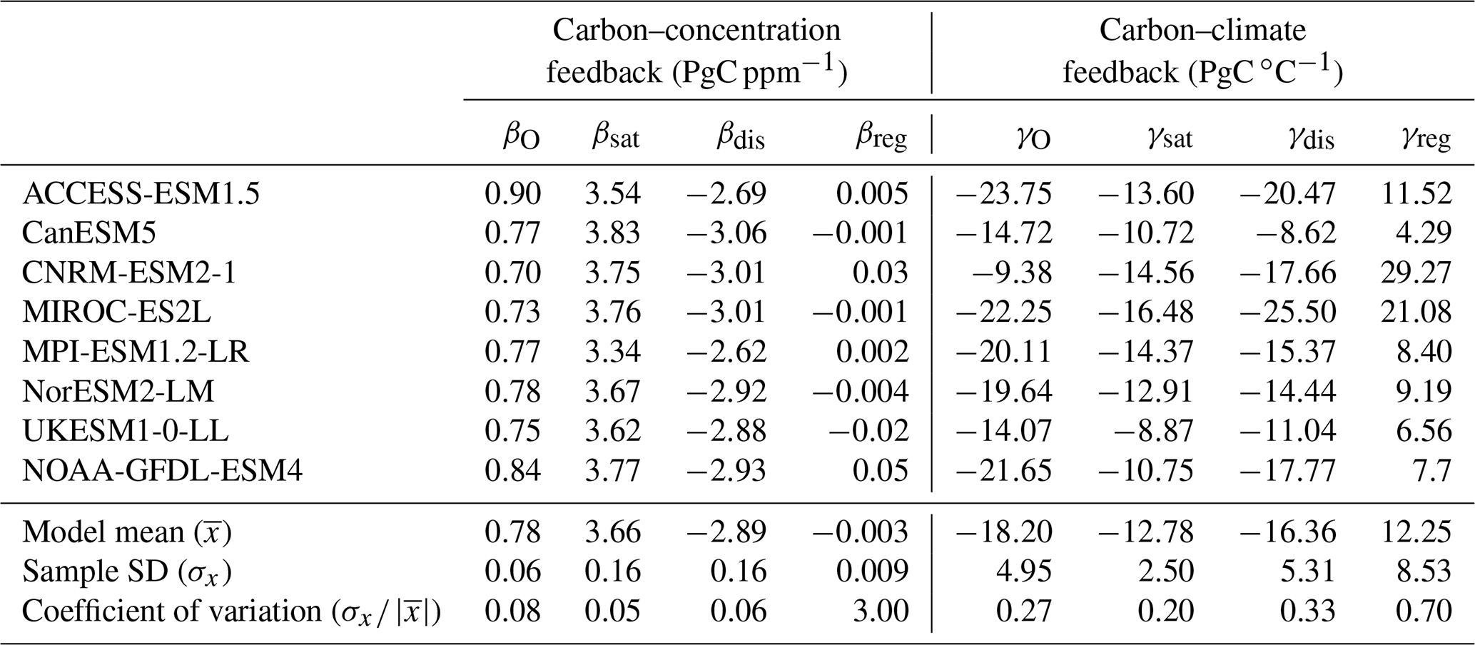
The atmospheric component of BCC-CSM2-MR has a T106 horizontal resolution of approximately 1.125∘ and 46 vertical levels in a hybrid sigma–pressure vertical coordinate system with the top level at 1.459 hPa. The ocean component resolution of BCC-CSM2-MR is 1∘ longitude by latitude between 30∘ S and 30∘ N which increases to 1∘ latitude at 60∘ S and 60∘ N and nominally 1∘ polarward with tripolar coordinates, and there are 40 z levels in the vertical plane.
The atmospheric component model BCC-AGCM3-MR in BCC-CSM2-MR is developed from its previous CMIP5 version (Wu et al., 2008). The main updates include a modification of deep convection parameterization, a new scheme for cloud fraction, indirect effects of aerosols through clouds and precipitation, and the gravity wave drag generated by deep convection (Wu et al., 2019). Atmospheric CO2 concentration in BCC-AGCM3-MR for this work is a prognostic variable and calculated through a budget equation which considers advective transport in the atmosphere, anthropogenic CO2 emissions, and interactive CO2 fluxes at the interfaces with land and ocean. But chemical processes are not taken into account. The terrestrial carbon cycle in BCC-AVIM2 (Li et al., 2019) operates through a series of biochemical and physiological processes acting on the photosynthesis and respiration of vegetation and takes into account carbon loss due to turnover and mortality of vegetation and CO2 release into the atmosphere through soil respiration. The vegetation litter on the ground surface and in the soil is divided into eight terrestrial carbon pools (surface structural, surface metabolic, surface microbial, soil structural, soil metabolic, soil microbial, slow, and passive carbon pools) according to the timescale of the decomposition of carbon in each pool and the transfers between different pools. Allocation to and from the three vegetation biomass pools (leaf, stem, root) leads to dynamic vegetation that in turn produces litterfall and which ultimately transfers carbon to soil organic matter. The allocation of carbon to the three vegetation biomass pools is dependent on light availability, water stress, and the phenology stages of the canopy and follows the formulations of Arora and Boer (2005).
The biogeochemistry module to simulate the ocean carbon cycle in MOM4_L40 is based on the protocols from the Ocean Carbon-Cycle Model Intercomparison Project Phase 2 (OCMIP2; http://ocmip5.ipsl.jussieu.fr/OCMIP/phase2/, last access: 15 December 2019). The OCMIP biogeochemistry module parameterizes the process of marine biology in terms of geochemical fluxes, without explicit representation of the marine ecosystem and food web processes, and includes five prognostic variables: phosphate, dissolved organic phosphorus, dissolved oxygen, dissolved inorganic carbon, and alkalinity. Ocean carbon cycle processes in BCC-CSM2-MR follow OCMIP, except for in parameterizing the export of organic matter from surface waters to deep oceans (Wu et al., 2013).
A4.3 Canadian Centre for Climate Modelling and Analysis (CCCma) fifth-generation Earth System Model, CanESM5
CanESM5 has evolved from its predecessor CanESM2 (Arora et al., 2011) that was used in the Coupled Model Intercomparison Project phase 5 (CMIP5). CanESM5 represents a major update to CanESM2 and is described in detail in Swart et al. (2019). The major changes relative to CanESM2 are the implementation of completely new models for the ocean, sea ice, and marine ecosystems and a new coupler. The resolution of CanESM5 (T63 or in the atmosphere and in the ocean) remains similar to CanESM2 and is at the lower end of the spectrum of CMIP6 models. The atmospheric component of CanESM5 is represented by version 5 of the Canadian Atmospheric Model (CanAM5) and has several improvements relative to its predecessor, CanAM4 (von Salzen et al., 2013), including changes to aerosol, clouds, radiation, land surface, and lake processes. CanAM5 uses a triangular spectral truncation in the model dynamical core, with an approximate horizontal resolution of 2.8∘ in latitude and longitude. It uses a hybrid vertical coordinate system with 49 levels between the surface and 1 hPa, with a vertical resolution of about 100 m near the surface. Relative to the 35 levels used in CanESM2 most of the additional 14 levels were added in the upper troposphere and stratosphere.
The land surface in CanESM5 is modelled using the Canadian Land Surface Scheme (CLASS; Verseghy, 2000) and the Canadian Terrestrial Ecosystem Model (CTEM; Arora and Boer, 2005, 2010), which together form the land component of CanESM5. CLASS and CTEM simulate the physical and biogeochemical land surface processes, respectively, and together they calculate fluxes of energy, water, CO2, and wetland CH4 emissions at the land–atmosphere boundary. Over land, three permeable soil layers are used with default thicknesses of 0.1, 0.25, and 3.75 m for which liquid and frozen soil moisture and temperature are prognostically calculated. The depth to bedrock is specified on the basis of the global dataset which reduces thicknesses of the permeable soil layers where soil depth is less than 4.1 m. Snow is represented using one layer, whose snow water equivalent and temperature are modelled prognostically. The introduction of dynamic wetlands and their methane emissions is a new biogeochemical process added since the CanESM2 (Arora et al., 2018). The nitrogen cycle over land is not represented but the parameterization of photosynthesis downregulation as CO2 increases is included. The magnitude of the parameter representing this downregulation is increased in CanESM5 compared to CanESM2, following Arora and Scinocca (2016), who found the best value of this parameter that reproduced various aspects of the historical carbon budget for CanESM4.2 (a model version more similar to CanESM2 than CanESM5). Other than wetlands and the changes to the strength of the CO2 fertilization effect, the remaining terrestrial ecosystem processes are represented in the same way as in CanESM2.
The physical ocean component of CanESM5 is based on Nucleus for European Modelling of the Ocean (NEMO) version 3.4.1. It is configured on the tripolar ORCA1 C grid with 45 z-coordinate vertical levels, varying in thickness from ∼6 m near the surface to ∼250 m in the abyssal ocean. The horizontal resolution is based on a 1∘ Mercator grid, varying with the cosine of latitude, with a refinement of the meridional grid spacing to near the Equator. Two modifications have been introduced to the NEMO mesoscale and small-scale mixing physics in CanESM5, and these are detailed in Swart et al. (2019). Sea ice is represented using the LIM2 sea ice model (Fichefet and Morales Maqueda, 1997; Bouillon et al., 2009), which is run within the NEMO framework.
The ocean carbon cycle is represented using the Canadian Model of Ocean Carbon (CMOC), which was developed for earlier versions of CanESM (Christian et al., 2010; Arora et al., 2011), and includes carbon chemistry and biology. The biological component is a simple nutrient–phytoplankton–zooplankton–detritus (NPZD) model, with fixed Redfield stoichiometry, and simple parameterizations of iron limitation, nitrogen fixation, and export flux of calcium carbonate.
A4.4 Community Earth System Model version 2 (CESM2)
CESM2 (Danabasoglu et al., 2020) contains substantial improvements on CESM1. The resolution remains the same as in CESM1 (0.9∘ latitude × 1.25∘ longitude for the atmosphere and land with 32 vertical atmospheric levels and 25 ground levels and for the ocean). The Community Atmosphere Model version 6 includes many changes to the representation of physical processes with the primary change being the inclusion of the Cloud Layers Unified By Binormals (CLUBB) unified turbulence scheme.
The CESM2 ocean component (Parallel Ocean Program version 2, POP2) is largely the same as that used in CESM1 except with a new parameterization for mixing effects in estuaries along with several other numerical and physics improvements. The sea ice model is CICE version 5.1.2 (CICE5; Hunke et al., 2015) . Ocean biogeochemistry is represented by the Marine Biogeochemistry Library (MARBL). MARBL represents multiple nutrient colimitations (N, P, Si, and Fe). It includes three explicit phytoplankton functional groups (diatoms, diazotrophs, and picophytoplankton and nanophytoplankton), one implicit phytoplankton group (calcifiers), and one zooplankton group. MARBL includes prognostic carbonate chemistry and simulates sinking particulate organic matter. Major updates relative to CESM1 include a representation of subgrid-scale variations in light and variable C : P stoichiometry. The atmospheric deposition of iron is computed prognostically in CESM2 as a function of dust and black carbon deposition simulated by CAM6. Riverine nutrient, carbon, and alkalinity fluxes are supplied to the ocean from a dataset.
The land component is the Community Land Model version 5 (CLM5; Lawrence et al., 2019) which simulates land water, energy, momentum, and carbon and nitrogen cycling. CLM5 includes an extensive suite of new and updated processes and parameterizations that collectively improve the model's hydrological, biogeochemical, and ecological realism and enhance the representation of anthropogenic land use activities on climate and the carbon cycle. The primary updates are as follows with details, references, and additional updates described and listed in Lawrence et al. (2019): (1) updated parameterizations and structure for hydrology and snow (spatially explicit soil depth, dry surface layer, revised groundwater scheme, revised canopy interception and canopy snow processes, updated fresh snow density, and inclusion of the Model for Scale Adaptive River Transport); (2) a plant hydraulics scheme to more mechanistically represent plant water use and limitation; (3) vertically resolved soil biogeochemistry with base organic matter decomposition rates varying with depth and modified by soil temperature, water, and oxygen limitation and nitrification and denitrification updated as in the CENTURY model; (4) a methane production, oxidation, and emissions model; (5) improved representation of plant N dynamics to address deficiencies in CLM4 through the introduction of flexible plant carbon : nitrogen (C:N) stoichiometry which avoids the problematic CLM4 separation of potential and actual plant productivity, explicitly simulating the photosynthetic capacity response to environmental conditions through the Leaf Utilization of Nitrogen for Assimilation (LUNA) module and accounting for how N availability affects plant productivity through the Fixation and Uptake of Nitrogen (FUN) module which determines the C costs of N acquisition; methane emissions and oxidation from natural land processes; (6) a global active crop model with six crop types and time-evolving irrigated areas and industrial fertilization rates; (7) updated canopy processes including a revised canopy radiation scheme and canopy scaling of leaf processes, colimitations on photosynthesis, and updated stomatal conductance; (8) a new fire model that includes representation of natural and anthropogenic ignition sources and suppression along with agricultural, deforestation, and peat fires; and (9) inclusion of carbon isotopes.
A4.5 Centre National de Recherches Météorologiques (CNRM) CNRM-ESM2-1
CNRM-ESM2-1 is the second-generation Earth System model developed by CNRM and Centre Européen de Recherche et de Formation Avancée en Calcul Scientifique (CERFACS) for CMIP6 (Séférian et al., 2019).
The atmosphere component of CNRM-ESM2-1 is based on version 6.3 of the global spectral model ARPEGE-Climat (ARPEGE-Climat_v6.3). ARPEGE-Climat resolves atmospheric dynamics and thermodynamics on a T127 triangular grid truncation that offers a spatial resolution of about 150 km in both longitude and latitude. CNRM-ESM2-1 employs a “high-top” configuration with 91 vertical levels that extend from the surface to 0.01 hPa in the mesosphere; 15 hybrid σ–pressure levels are available below 1500 m.
The surface state variables and fluxes at the surface–atmosphere interface are simulated by the SURFEX modelling platform version 8.0 over the same grid and with the same time step as the atmosphere model. SURFEX v8.0 encompasses several submodules for modelling the interactions between the atmosphere, the ocean, the lakes, and the land surface. Over the land surface, CNRM-ESM2-1 uses the ISBA-CTRIP land surface modelling system (http://www.umr-cnrm.fr/spip.php?article1092&lang=en, last access: 15 December 2019) to solve energy, carbon, and water budgets at the land surface (Decharme et al., 2019; Delire et al., 2019). Its physical core explicitly solves the one-dimensional Fourier's and Darcy's laws throughout the soil, accounting for the hydraulic and thermal properties of soil organic carbon. It uses a 12-layer snow model of intermediate complexity that allows for separate water and energy budgets for the soil and the snowpack. It accounts for a dynamic river flooding scheme in which floodplains interact with the soil and the atmosphere through free-water evaporation, infiltration, and precipitation interception and a two-dimensional diffusive groundwater scheme to represent unconfined aquifers and upward capillarity fluxes into the superficial soil. More details on these physical aspects can be found in Decharme et al. (2019).
To simulate the land carbon cycle and vegetation–climate interactions, ISBA-CTRIP simulates plant physiology, carbon allocation and turnover, and carbon cycling through vegetation, litter, and soil. It includes a module for wild fires, land use and land cover changes, and carbon leaching through the soil and transport of dissolved organic carbon to the ocean. Leaf photosynthesis is represented by the semiempirical model proposed by Goudriaan et al. (1985). Canopy-level assimilation is calculated using a 10-layer radiative transfer scheme including direct and diffuse radiation. Vegetation in ISBA is represented by four carbon pools for grasses and crops (leaves, stem, roots and a nonstructural carbohydrate storage pool) with two additional pools for trees (aboveground wood and coarse roots). Leaf phenology results directly from the carbon balance of the leaves. The model distinguishes 16 vegetation types (10 tree and shrub types, 3 grass types, and 3 crop types) alongside desert, rocks, and permanent snow. In the absence of nitrogen cycling within the vegetation, an implicit nitrogen limitation scheme that reduces specific leaf area with increasing CO2 concentration was implemented in ISBA following the meta-analysis of Yin (2002). Additionally, there is an ad hoc representation of photosynthesis downregulation. The litter and soil organic matter module is based on the soil carbon part of the CENTURY model (Parton et al., 1988). The four litter and three soil carbon pools are defined based on their location aboveground or belowground and potential decomposition rates. The litter pools are supplied by the flux of dead biomass from each biomass reservoir (turnover). Decomposition of litter and soil carbon releases CO2 (heterotrophic respiration). During the decomposition process, some carbon is dissolved by water slowly percolating through the soil column. This dissolved organic carbon is transported by the rivers to the ocean. A detailed description of the terrestrial carbon cycle can be found in Delire et al. (2019).
The ocean component of CNRM-ESM2-1 is the Nucleus for European Modelling of the Ocean (NEMO) version 3.6 (Madec et al., 2016) which is coupled to both the Global Experimental Leads and ice for ATmosphere and Ocean (GELATO) sea ice model (Salas Mélia, 2002) version 6 and also the marine biogeochemical model Pelagic Interactions Scheme for Carbon and Ecosystem Studies version 2 gas (PISCESv2-gas). NEMOv3.6 operates on the ORCA1L75 grid (Mathiot et al., 2017) which offers a nominal resolution of 1∘ to which a latitudinal grid refinement of is added in the tropics; this grid describes 75 ocean vertical layers using a vertical z∗ coordinate with partial step bathymetry formulation (Bernard et al., 2006).
The atmospheric chemistry scheme of CNRM-ESM2-1 is Reactive Processes Ruling the Ozone Budget in the Stratosphere version 2 (REPROBUS-C_v2). This scheme resolves the spatial distribution of 63 chemistry species but does not represent the low-troposphere ozone nonmethane hydrocarbon chemistry. CNRM-ESM2-1 also includes an interactive tropospheric aerosol scheme included in the atmospheric component ARPEGE-Climat. This aerosol scheme, named Tropospheric Aerosols for ClimaTe In CNRM (TACTIC_v2), represents the main anthropogenic and natural aerosol species of the troposphere.
The ocean biogeochemical component of CNRM-ESM2-1 uses the PISCESv2-gas model, which derives from PISCESv2 as described in Aumont et al. (2015). PISCESv2-gas simulates the distribution of five nutrients (from macronutrients nitrate, ammonium, phosphate, and silicate to the micronutrient iron) which regulate the growth of two explicit phytoplankton classes (nanophytoplankton and diatoms). Dissolved inorganic carbon (DIC) and alkalinity (Alk) are involved in the computation of the carbonate chemistry, which is resolved by routines to model the ocean carbonate system version 2 (mocsy 2.0; Orr and Epitalon, 2015) in PISCESv2-gas. The use of mocsy 2.0 enables a better and faster resolution of the ocean carbonate chemistry at thermodynamic equilibria. Oxygen is prognostically simulated using two different oxygen-to-carbon ratios, one when ammonium is converted to or mineralized from organic matter and the other when oxygen is consumed during nitrification. Their values have been set to 131∕122 and 32∕122, respectively.
At the ocean surface, PISCESv2-gas exchanges carbon, oxygen, dimethylsulfide (DMS), and nitrous oxide (N2O) tracers with the atmosphere using the revised air–sea exchange bulk as published by Wanninkhof (2014). PISCESv2-gas uses several boundary conditions which represent the supply of nutrients from five different sources: atmospheric deposition, rivers, sediment mobilization, sea ice, and hydrothermal vents.
A4.6 Institut Pierre Simon Laplace (IPSL) IPSL-CM6A-LR
IPSL-CM6A-LR is the coupled climate model of the Institut Pierre Simon Laplace. It results from the integration of the following components: the LMDZ atmospheric general circulation model (version 6A-LR; Hourdin et al., 2019), the NEMO oceanic model (version 3.6; Vancoppenolle et al., 2009; Aumont et al., 2015; Rousset et al., 2015; Madec et al., 2016), and the ORCHIDEE land surface model (version 2.0).
The atmospheric general circulation model LMDZ6A-LR builds onto its previous version that has notably incorporated advances in the parameterization of turbulence, convection, and clouds. More specifically, LMDZ6A-LR includes a turbulent scheme based on the prognostic equation for the turbulent kinetic energy that follows Yamada (1983), a mass flux representation of the organized structures of the convective boundary layer called the thermal plume model (Hourdin et al., 2002; Rio and Hourdin, 2008; Rio et al., 2010), and a parameterization of the cold pools or wakes created below cumulonimbus by the evaporation of convective rainfall (Grandpeix and Lafore, 2010; Grandpeix et al., 2010). It is based on a regular horizontal grid with 144 grid points regularly spaced in longitude and 142 in latitude, corresponding to a resolution of , and 79 vertical layers.
IPSL-CM6A-LR further includes NEMO (Nucleus for European Models of the Ocean), which is itself composed of three major building blocks: the ocean physics NEMO-OPA (Madec et al., 2016), the sea ice dynamics and thermodynamics NEMO-LIM3 (Vancoppenolle et al., 2009; Rousset et al., 2015), and the ocean biogeochemistry NEMO-PISCES (Aumont et al., 2015). The grid used has a nominal resolution of 1∘ in the zonal and meridional directions with a latitudinal grid refinement of in the tropics. Vertical discretization uses a partial step formulation (Bernard et al., 2006), which ensures a better representation of bottom bathymetry, with 75 levels. The initial layer thicknesses increase nonuniformly from 1 m at the surface to 10 m at 100 m depth and reach 200 m at the bottom and are subsequently time-dependent. NEMO-PISCES (Aumont et al., 2015) models the lower trophic levels of the marine ecosystem (phytoplankton, microzooplankton, and mesozooplankton) and the biogeochemical cycles of carbon and of the main nutrients (P, N, Fe, and Si). This model also computes air–sea carbon fluxes.
Finally, IPSL-CM6A-LR includes ORCHIDEE, a global process-based terrestrial biosphere model (Krinner et al., 2005) that calculates carbon, water, and energy fluxes between the land surface and the atmosphere. Photosynthesis and all components of the surface energy and water budgets are calculated at a 15 min resolution, while the dynamics of the carbon storage (including carbon allocation in plant reservoirs, soil carbon dynamics, and litter decomposition) are resolved on a daily basis. Photosynthesis depends on light availability and CO2 concentration, soil moisture, and temperature and is parameterized based on Farquhar et al. (1980) and Collatz et al. (1992) for C3 and C4 plants, respectively. In the absence of an explicit representation of the nitrogen cycle, this latest version of ORCHIDEE includes a downregulation capability that models a reduction in the terrestrial photosynthesis rates as a function of CO2 concentration. While the N and C cycles interact in multiple ways, a key aspect of these interactions is the limitation of carbon uptake by nitrogen availability, especially under increasing atmospheric CO2 concentrations. The downregulation parameterization models a reduction in the maximum photosynthetic rate as the atmospheric CO2 concentrations increase using a logarithmic function of the CO2 concentration relative to 380 ppm (Sellers et al., 1996). The PFT-dependent parameters of this parameterization are chosen to broadly reproduce the change in GPP observed at the free-air CO2 enrichment (FACE) experiment sites (Norby and Zak, 2011). In ORCHIDEE, the spatial distribution of vegetation is represented using 15 plant functional types (PFTs; Prentice et al., 1992; Cramer, 1997; Wullschleger et al., 2014). More precisely these PFTs are decomposed into three groups according to their physiological behaviour under similar climate conditions: tall vegetation (forests) represented by eight PFTs, short vegetation (grasses and crops) represented by six PFTs, and bare soil. The fractional coverage of these PFTs varies geographically. A soil type is associated with each one of these three PFT groups. This three-group partitioning allows for the dividing of each grid box into three tiles for which an independent hydrological budget is calculated, using the 11-layer physically based hydrology scheme. In ORCHIDEE the wood harvest product from the LUHv2h database is used in addition to the annual land cover maps.
A4.7 Team MIROC (Japan Agency for Marine-Earth Science and Technology, the University of Tokyo, the National Institute for Environmental Studies) MIROC-ES2L
MIROC-ES2L (Hajima et al., 2020) is based on the global climate model MIROC5.2 (Tatebe et al., 2018), which is a minor updated version of MIROC5 used for CMIP5 (Watanabe et al., 2010). The physical core shares almost the same structure and characteristics with the latest model MIROC6 (Tatebe et al., 2019), except for the atmospheric spatial resolution and treatment of cumulus clouds. This model interactively couples an atmospheric general circulation model (CCSR-NIES AGCM; Tatebe et al., 2019) including an on-line aerosol component (SPRINTARS; Takemura et al., 2000), an ocean general circulation model (GCM) with a sea ice component (COCO; Hasumi, 2015), and a land physical surface model (MATSIRO; Takata et al., 2003). The land and ocean biogeochemical components are represented by VISIT (Ito and Inatomi, 2012) and OECO2 (Hajima et al., 2020), respectively, which are interactively coupled to the atmospheric component. There exists another branched version that has an atmospheric chemistry component with a finer atmospheric grid (MIROC-ES2H), but it was not used in this study.
The atmospheric grid resolution is approximately 2.81∘ with 40 vertical levels between the surface and about 3 hPa. For the ocean, the model employs a tripolar coordinate system with 62 vertical levels. To the south of 63∘ N, the ocean model has longitudinal grid spacing of about 1∘, while the meridional grid spacing varies from about 0.5∘ near the Equator to 1∘ in the midlatitudes. Over the Arctic ocean the grid resolution is even finer following the tripolar coordinate system. The physical terrestrial component resolves the vertical soil profile with six layers down to a 14 m depth, with two types of land use tiles (agriculture and nonagriculture). Terrestrial biogeochemical component considers two layers of soil organic matter (the upper litter layer and the lower humus layer), with five types of land use tiles (primary vegetation, secondary vegetation, urban, crop, and pasture).
The terrestrial biogeochemical component covers major processes relevant to the global carbon cycle, with vegetation (leaf, stem, and root), litter (leaf, stem, and root), and humus (active, intermediate, and passive) pools and with a static biome distribution. Details on carbon cycle processes in the model can been found in Ito and Oikawa (2002). The N cycle is simulated with N pools of vegetation (canopy and structural), organic soil (litter, humus, and microbe), and inorganic nitrogen (ammonium and nitrate). The model considers two major nitrogen influxes into the ecosystem (biological nitrogen fixation and external nitrogen inputs). Fluxes out of the land ecosystem in the model are N2 or N2O emissions, leaching, NH3 emissions, and other emission-like volatilization from land use product pools. For installing into MIROC-ES2L, the terrestrial ecosystem processes were modified such that photosynthetic capacity is controlled by leaf N concentration. Processes associated with land use change are also modified to take full advantage of the CMIP6 LUC forcing dataset. Further details can be found in Hajima et al. (2020).
The new ocean biogeochemical component model, OECO2, is a NPZD-type model and modified from the previous model (Watanabe et al., 2011). The biogeochemical compartments of OECO2 are nitrate, phosphate, dissolved iron, dissolved oxygen, two types of phytoplankton (nondiazotroph and diazotroph), zooplankton, and particulate detritus. There exist other compartments of dissolved inorganic carbon (DIC), total alkalinity, calcium, calcium carbonate, and N2O. All organic materials have an identical elemental stoichiometric ratio. The model considers external nutrient inputs (atmospheric N and Fe deposition, inorganic N and P from rivers, biological N fixation, Fe input from ocean bottom and shelf) and nutrient loss (denitrification for N and loss into sediment for N, P, and Fe). The emission, transportation, and deposition processes of iron are explicitly simulated by the atmospheric aerosol component.
A4.8 Max Planck Institute for Meteorology (MPI) MPI-ESM1.2-LR
The MPI-ESM1.2-LR model (Mauritsen et al., 2019) consists of ocean, atmosphere, land, and sea ice components which are connected via a coupler analogous to the predecessor MPI-ESM versions (Giorgetta et al., 2013). The atmosphere model, ECHAM6.3, at the LR resolution has a spectral truncation at T63 or approximately 200 km grid spacing with 47 vertical levels. It is directly coupled to the land model, JSBACH3.2, through surface exchange of mass, momentum, and heat. The ocean general circulation model, MPIOM1.6 in MPI-ESM1.2-LR, runs on a bipolar grid GR1.5 and has 40 unevenly placed levels. It computes transport of tracers of the ocean biogeochemistry model HAMOCC6 (Ilyina et al., 2013; Paulsen et al., 2017). The MPI-ESM-LR configuration computes 45–85 model years per physical day enabling new simulations which were not feasible previously, such as for instance, large ensemble simulations (Maher et al., 2019) or millennial-scale simulations with an interactive carbon cycle (Brovkin et al., 2019).
Terrestrial vegetation in JSBACH includes vegetation dynamics which interacts with land use changes (Reick et al., 2013), accounting for the latest changes in the land use harmonization dataset by Hurtt et al. (2006). The new SPITFIRE model simulates burned area and carbon emissions to the atmosphere due to wildfires and anthropogenic fires (Lasslop et al., 2014), replacing the old global fire parameterization used in the CMIP5 model. The soil carbon model Yasso simulates the dynamics of four fast soil carbon pools, which are different for leaf and woody litter types, plus a slow humus pool (Goll et al., 2015). Nitrogen and carbon pools are coupled based on CO2-induced nitrogen limitation (Goll et al., 2017).
The ocean biogeochemistry model HAMOCC6 has been extended compared to the previous version described in Ilyina et al. (2013) to explicitly resolve nitrogen-fixing cyanobacteria as an additional prognostic phytoplankton class (Paulsen et al., 2017). This allows for the capture of the response of N2 fixation and ocean biogeochemistry to changing climate conditions. Additionally, updates of existing processes have been performed. This includes for instance the addition of a vertically varying settling rate for detritus following the formulation by Martin et al. (1987). Finally some empirical relationships in the parameterized processes have been updated to follow recommendations of the C4MIP and OMIP protocols (Jones et al., 2016; Orr et al., 2017). The full overview of changes in HAMOCC is given in Mauritsen et al. (2019).
A4.9 Geophysical Fluid Dynamics Laboratory (GFDL) NOAA-GFDL-ESM4
GFDL-ESM4.1 is a comprehensive, fully coupled Earth system model developed by NOAA's Geophysical Fluid Dynamics Laboratory with a fully interactive carbon cycle and interactive atmospheric chemistry (Dunne et al., 2020) that builds on previous-generation modelling efforts of the carbon cycle (ESM2 series; Dunne et al., 2012, 2013) and atmospheric chemistry (CM3; Donner et al., 2011) along with increased resolution and improved numerics and physics, akin to the GFDL's fourth-generation coupled climate model (CM4.0; Held et al., 2019), and representation of additional Earth system processes.
The atmospheric component, GFDL AM4.1, is based on the third-generation finite-volume cube-sphere dynamical core (FV3; Lin, 2004) with a ∼100 km horizontal resolution and 49 vertical levels. The model top is located at ∼0.01 hPa to resolve the stratosphere. AM4.1 shares the critical developments in model physics with the AM4.0 model (Zhao et al., 2018), including radiation, convection, and clouds. AM4.1 differs from the AM4.0 model in its enhanced vertical resolution and its more explicit representation of atmospheric chemistry that motivated a separate radiative and gravity wave tuning.
AM4.1 includes interactive tropospheric and stratospheric gas-phase and aerosol chemistry represented through 77 prognostic (transported) tracers and 41 diagnostic (nontransported) chemical tracers. The tropospheric chemistry includes reactions for the oxidation of methane among other volatile organic compounds. The stratospheric chemistry accounts for the major ozone loss cycles and heterogeneous reactions on liquid and solid stratospheric aerosols.
Land hydrology and ecosystem dynamics are represented by the GFDL Land Model version 4.1 (LM4.1, Shevliakova et al., 2020) and build on the previous-generation LM3.1 model (Milly et al., 2014). Soil carbon dynamics and biogeochemistry are represented through the CORPSE model (Sulman et al., 2019) with an explicit treatment of soil microbes. LM4.1 also includes a new fire model FINAL (Rabin et al., 2018). Vegetation dynamics are represented by the second-generation age–height-structured approach, the perfect plasticity approximation (PPA; Weng et al., 2015; Martinez Cano et al., 2020). Allometric constraints and competition enable the simulation of size structure and carbon fluxes in dynamic vegetation. There are six carbon pools in LM4.1 representing leaves, fine roots, heartwood, sapwood, seeds, and nonstructural carbon. Litter is broken into leaf, fine roots, and coarse-wood categories. Soil has 20 vertical levels each with its own prognostic state for energy, water, and soil carbon variables. There are five types of vegetation in LM4.1 representing C3 grass, C4 grass, tropical trees, temperate deciduous trees, and cold evergreen trees. A combination of these vegetation types could coexist. The model also includes a new treatment of stomatal conductance and plant hydraulics. The vegetation state is used to drive a dust emission model that is coupled with the atmosphere for transport. The ESM4 implementation of LM4.1 does not include an interactive nitrogen cycle.
The ocean biogeochemical component of ESM4 is version 2 of the Carbon, Ocean Biogeochemistry and Lower Trophics (COBALTv2) model (Stock et al., 2014b). COBALTv2 uses 33 tracers to represent carbon, alkalinity, oxygen, nitrogen, phosphorus, iron, silica, calcite, and lithogenic mineral cycling within the ocean. Relative to previous-generation ocean biogeochemistry models developed at the GFDL, COBALTv2 includes an enhanced representation of plankton food web dynamics to resolve the flow of energy from phytoplankton to fish (Stock et al., 2014a) and enhance the model's capacity to resolve linkages between food webs and biogeochemical cycles. COBALTv2 explicitly includes small, large (split into diatoms and nondiatoms), and diazotrophic phytoplankton groups; three zooplankton groups; bacteria; and three labilities of dissolved organic matter. Other updates include a temperature dependence for sinking organic matter remineralization (Laufkötter et al., 2017), the addition of semilabile dissolved organic material and carbonate chemistry calculations based on the open-source mocsy 2.0 (Orr and Epitalon, 2015).
Data from the NOAA-GFDL-ESM4 model used in the analysis presented in this paper are accessible via the Earth System Grid Federation (ESGF) for the 1pctCO2 (Krasting et al., 2019b) simulation and for its radiatively and biogeochemically coupled configurations (Krasting et al., 2019a).
A4.10 Norwegian Climate Centre (NCC) NorESM2-LM
The NorESM2-LM (Seland et al., 2020) is based on the latest release of the Community Earth System Model (CESM2.1), whose development is supported by the National Center for Atmospheric Research in the United States. NorESM2 keeps the original land and sea ice components of CESM2.1 (i.e. CLM5 and CICE5, respectively). The atmospheric component is CAM6 (as in CESM) but with modifications regarding the energy and angular momentum conservation. Further, the atmospheric aerosol module of CAM6 has been replaced by the scheme developed by the Norwegian Meteorological Institute. The ocean physical and biogeochemical components of NorESM2 are the isopycnal ocean circulation and carbon cycle components updated from NorESM1 version (Tjiputra et al., 2013; Schwinger et al., 2016)
The CLM5 (Community Land Model version 5) prognostically simulates the carbon and nitrogen cycles, which include natural vegetation, crops, and soil biogeochemistry. The carbon and nitrogen budgets comprise leaf, live-stem, dead-stem, live-coarse-root, dead-coarse-root, fine-root, and grain pools. Each of these pools has short-term and long-term storage of nonstructural carbohydrates and labile nitrogen. In addition to the vegetation pools, CLM includes a series of decomposing carbon and nitrogen pools as vegetation successively breaks down into coarse woody debris and/or litter and subsequently into soil organic matter. Details on the CLM5 models are available in Lawrence et al. (2019).
Similar to the earlier version, the ocean carbon cycle component in NorESM2 is based on the Hamburg Ocean Carbon Cycle (HAMOCC; Maier-Reimer et al., 2005) model, which has been coupled to an isopycnic ocean general circulation model. The current version includes new processes and refined parameterizations, as well as new diagnostic tracers. The ecosystem model is based on an NPZD-type model with multinutrient limitation in its phytoplankton growth formulation. Riverine fluxes of inorganic and organic carbon as well as nutrients are now implemented. Unlike the earlier version, the sea-to-air dimethyl sulfate (DMS) fluxes alter the atmospheric radiative forcing and hence the climate–carbon cycle feedback. More details on the ocean carbon cycle of NorESM2 are available in Tjiputra et al. (2020).
A4.11 The United Kingdom Community Earth System Model, UKESM1-0-LL
UKESM1-0-LL (Sellar et al., 2019) is based upon the HadGEM3-GC3.1 (Williams et al., 2018) global climate model which includes coupled ocean, atmosphere, land, and sea ice components. The atmosphere component is the Unified Model with a resolution of 1.875∘ by 1.25∘ with 85 vertical levels up to a model top of 90 km (Walters et al., 2019) and includes a modal aerosol scheme (Mann et al., 2010). The ocean component uses the NEMO dynamical ocean at 1∘ resolution with 75 vertical levels (Storkey et al., 2018). The sea ice component uses CICE on the same grid as the ocean with five ice thickness categories (Ridley et al., 2018). The land component uses the JULES land surface model (Wiltshire et al., 2020); however, the land surface configuration is substantially updated for UKESM. The primary differences between the physical and Earth system models are the inclusion of a terrestrial carbon and nitrogen cycle (Wiltshire et al., 2020), ocean biogeochemistry (Yool et al., 2013), and a tropospheric–stratospheric chemistry model. Atmospheric chemistry in UKESM1 is simulated by the UKCA chemistry and aerosol model with the specific configuration being a combination of tropospheric (O'Connor et al., 2014) and stratospheric chemistry (Morgenstern et al., 2009, 2017).
Terrestrial biogeochemistry is represented by the JULES-ES model (Wiltshire et al., 2020). The land surface is represented by 13 plant functional types (PFTs) including 4 managed crop and pasture land types. The height, leaf area index, and spatial distribution of the PFTs are dynamically simulated by the TRIFFID dynamic global vegetation model (DGVM; Cox, 2001). Soil carbon is represented by the four-pool RothC scheme (Coleman and Jenkinson, 1999). Terrestrial carbon uptake may be limited by the availability of nitrogen. Nitrogen does not directly affect photosynthetic capacity through leaf N concentrations but acts indirectly by controlling the biomass and leaf area index within the TRIFFID DGVM. A second mechanism acts through soil carbon by limiting the decomposition of litter into soil carbon in the RothC model. The vegetation model includes the retranslocation of nitrogen during the senescence of leaves and roots into a labile pool to supply nutrients for the following seasonal leaf-out. The soil model simulates mineralization and immobilization with mineralized nitrogen becoming available for plant uptake and ecosystem loss. Inorganic nitrogen is represented by a single grid box pool to which all PFTs have equal access. Nitrogen deposition is prescribed from ancillary data.
Land use change is represented by the application of time-varying fields of crop and pasture to the DGVM, which allocates space dynamically to C3 and C4, and crop and pasture types. Pasture is represented as natural grass, whereas crops include a harvest parameterization and are fertilized. Biogenic volatile organic compound (BVOC) emissions from vegetation are simulated and affect the formation of secondary organic aerosols. Mineral dust is emitted from bare soil and acts as both an aerosol and a fertilizer to the ocean.
Ocean biogeochemistry is represented by MEDUSA-2 (Yool et al., 2013), which resolves a dual size-structured ecosystem of small (nanophytoplankton and microzooplankton) and large (microphytoplankton and mesozooplankton) components. This explicitly includes the biogeochemical cycles of nitrogen, silicon, and iron nutrients as well as the cycles of carbon, alkalinity, and dissolved oxygen. Large phytoplankton are treated as diatoms and utilize silicic acid in addition to nitrogen, iron, and carbon. Like the living components, the detrital components are split into two size classes. At the seafloor, MEDUSA-2 resolves five reservoirs to temporarily store sinking organic material reaching the sediment. The model's nitrogen, silicon, and alkalinity cycles are closed and conservative (e.g. no riverine inputs), while the other three cycles (carbon, iron, oxygen) are open. The ocean's iron cycle includes aeolian (land-derived dust) and benthic sources, and is depleted by scavenging. The ocean's carbon cycle exchanges CO2 with the atmosphere. The ocean's oxygen cycle exchanges oxygen with the atmosphere, and dissolved oxygen is additionally created by primary production and depleted by remineralization. Ocean biogeochemistry also feeds back on the atmosphere through the production of marine DMS and marine organic aerosols.
A5 Contribution of uncertainties in and to the TCRE.
The uncertainty in the TCRE, as indicated by its standard deviation (σTCRE), can be represented in terms of the standard deviation of (σΔT), the standard deviation of (σE), and their means and across the 11 CMIP6 models. Since and are nearly independent (correlation between these two quantities is only 0.02 across the 11 CMIP6 models considered here), we can write
which allows us to calculate contributions of and to σTCRE.
The data used here are from the CMIP6 simulations performed by the various modelling groups and available from the CMIP6 archive (https://esgf-node.llnl.gov/search/cmip6).
The following variables were used from the models reported in Table 2 and for the three experiments (1pctCO2, 1pctCO2-bgc, 1pctCO2-rad). Over land tas, co2, netAtmosLandCO2Flux, gpp, npp, rhSoil, rhLitter, cVeg, cSoil, and cLitter were used. Over ocean fgco2, dissic, so, thetao, talk, po4, no3, si, o2, areacello_Ofx, volcello_Ofx, basin_Ofx, and sftlf_fx were used.
At the CMIP6 archive site (https://esgf-node.llnl.gov/search/cmip6) searching for a given model, a given experiment, and a given variable name will yield the link to the dataset that can be downloaded. Although annual values are used for analysis in this paper, the CMIP6 data archive typically provides monthly values for most variables.
The supplement related to this article is available online at: https://doi.org/10.5194/bg-17-4173-2020-supplement.
VA wrote the majority of the manuscript and performed the analysis over land. AK and RW performed the analysis over the ocean and wrote sections related to the ocean and TCRE. VA, CDJ, PF, VB, TI, RW, JS, and LB attended the Bern Carbon Cycle Workshop in April 2018 where the extended framework for analyzing land and ocean carbon cycle feedbacks was developed. CDJ reviewed and contributed to various sections of the paper. VB, JS, JT, JC, and RS reviewed various sections of the paper and provided revised text for those sections. Model descriptions were provided by co-authors who represent the various climate modelling groups. These co-authors were also responsible for processing output from their respective models and providing data in ready-to-use format.
The authors declare that they have no conflict of interest.
The framework analysis outlined in this paper was developed at the workshop held in Bern, Switzerland, in April 2018, officially endorsed by the Grand Challenge “Carbon Feedbacks in the Climate System” of the World Climate Research Programme (WCRP) in cooperation with the Analysis, Integration and Modeling of the Earth System (AIMES) project of Future Earth. The paper contributes to the Coupled Climate Carbon Cycle Model Intercomparison (C4MIP) project of Coupled Models Intercomparison Project Phase 6 (CMIP6). The C4MIP website (http://c4mip.net/) is supported by the Max Planck Society.
We also thank one anonymous reviewer and Kirsten Zickfeld for their helpful comments on our paper and the handling editor Alexey Eliseev for taking on this paper.
CDJ and AJW were supported by the Joint UK BEIS/Defra Met Office Hadley Centre Climate Programme (GA01101). CDJ, VB, PF, RS, CD, and EJ acknowledge funding from the European Union's Horizon 2020 CRESCENDO project (grant agreement no. 641816). PF acknowledges funding from the European Union's Horizon 2020 “4C” project (grant agreement no. 821003). RS, CD, and EJ also acknowledge the H2020 CONSTRAIN under the grant agreement no. 820829. RGW and AK acknowledge support from the UK Natural Environmental Research Council, NE/N009789/1 and NE/T007788/1. CDK acknowledges support by the Director, Office of Science, Office of Biological and Environmental Research of the U.S. Department of Energy under contract DE-AC02-05CH11231 through the Regional and Global Model Analysis Program (RUBISCO SFA) and the Early Career Research Program. TH, MK, and KT acknowledge the support from TOUGOU, the Integrated Research Program for Advancing Climate Models (grant number JPMXD0717935715), through the Ministry of Education, Culture, Sports, Science, and Technology of Japan. JS and JT acknowledge support from The Research Council of Norway through projects KeyClim (grant no. 295046) and COLUMBIA (grant no. 275268) as well as support from the Bjerknes Centre for Climate Research through the project LOES.
This paper was edited by Alexey V. Eliseev and reviewed by Kirsten Zickfeld and one anonymous referee.
Ainsworth, E. A. and Long, S. P.: What have we learned from 15 years of free-air CO2 enrichment (FACE)?, A meta-analytic review of the responses of photosynthesis, canopy properties and plant production to rising CO2, New Phytol., 165, 351–372, https://doi.org/10.1111/j.1469-8137.2004.01224.x, 2005.
Arora, V. K. and Boer, G. J.: A parameterization of leaf phenology for the terrestrial ecosystem component of climate models, Glob. Change Biol., 11, 39–59, https://doi.org/10.1111/j.1365-2486.2004.00890.x, 2005.
Arora, V. K. and Boer, G. J.: Uncertainties in the 20th century carbon budget associated with land use change, Glob. Change Biol., 16, 3327–3348, 2010.
Arora, V. K. and Scinocca, J. F.: Constraining the strength of the terrestrial CO2 fertilization effect in the Canadian Earth system model version 4.2 (CanESM4.2), Geosci. Model Dev., 9, 2357–2376, https://doi.org/10.5194/gmd-9-2357-2016, 2016.
Arora, V. K., Scinocca, J. F., Boer, G. J., Christian, J. R., Denman, K. L., Flato, G. M., Kharin, V. V., Lee, W. G., and Merryfield, W. J.: Carbon emission limits required to satisfy future representative concentration pathways of greenhouse gases, Geophys. Res. Lett., 38, L05805, https://doi.org/10.1029/2010GL046270, 2011.
Arora, V. K., Boer, G. J., Friedlingstein, P., Eby, M., Jones, C. D., Christian, J. R., Bonan, G., Bopp, L., Brovkin, V., Cadule, P., Hajima, T., Ilyina, T., Lindsay, K., Tjiputra, J. F., and Wu, T.: Carbon–Concentration and Carbon–Climate Feedbacks in CMIP5 Earth System Models, J. Climate, 26, 5289–5314, https://doi.org/10.1175/JCLI-D-12-00494.1, 2013.
Arora, V. K., Melton, J. R., and Plummer, D.: An assessment of natural methane fluxes simulated by the CLASS-CTEM model, Biogeosciences, 15, 4683–4709, https://doi.org/10.5194/bg-15-4683-2018, 2018.
Aumont, O., Ethé, C., Tagliabue, A., Bopp, L., and Gehlen, M.: PISCES-v2: an ocean biogeochemical model for carbon and ecosystem studies, Geosci. Model Dev., 8, 2465–2513, https://doi.org/10.5194/gmd-8-2465-2015, 2015.
Bernard, B., Madec, G., Penduff, T., Molines, J.-M., Treguier, A.-M., Le Sommer, J., Beckmann, A., Biastoch, A., Böning, C., Dengg, J., Derval, C., Durand, E., Gulev, S., Remy, E., Talandier, C., Theetten, S., Maltrud, M., McClean, J., and De Cuevas, B.: Impact of partial steps and momentum advection schemes in a global ocean circulation model at eddy-permitting resolution, Ocean Dynam., 56, 543–567, https://doi.org/10.1007/s10236-006-0082-1, 2006.
Bernardello, R., Marinov, I., Palter, J. B., Sarmiento, J. L., Galbraith, E. D., and Slater, R. D.: Response of the Ocean Natural Carbon Storage to Projected Twenty-First-Century Climate Change, J. Climate, 27, 2033–2053, https://doi.org/10.1175/JCLI-D-13-00343.1, 2014.
Bi, D., Dix, M., Marsland, S., O'Farrell, S., Rashid, H., Uotila, P., Hirst, A., Kowalczyk, E., Golebiewski, M., Sullivan, A., Yan, H., Hannah, N., Franklin, C., Sun, Z., Vohralik, P., Watterson, I., Zhou, X., Fiedler, R., Collier, M., Ma, Y., Noonan, J., Stevens, L., Uhe, P., Zhu, H., Griffies, S., Hill, R., Harris, C., and Puri, K.: The ACCESS coupled model: description, control climate and evaluation, Aust. Meteor. Oceanogr. J., 63, 41–64, https://doi.org/10.22499/2.6301.004, 2013.
Boer, G. J. and Arora, V.: Geographic Aspects of Temperature and Concentration Feedbacks in the Carbon Budget, J. Climate, 23, 775–784, https://doi.org/10.1175/2009JCLI3161.1, 2010.
Bouillon, S., Maqueda, M. Á. M., Legat, V., and Fichefet, T.: An elastic–viscous–plastic sea ice model formulated on Arakawa B and C grids, Ocean Model., 27, 174–184, https://doi.org/10.1016/j.ocemod.2009.01.004, 2009.
Bounoua, L., Collatz, G. J., Sellers, P. J., Randall, D. A., Dazlich, D. A., Los, S. O., Berry, J. A., Fung, I., Tucker, C. J., Field, C. B., and Jensen, T. G.: Interactions between Vegetation and Climate: Radiative and Physiological Effects of Doubled Atmospheric CO2, J. Climate, 12, 309–324, https://doi.org/10.1175/1520-0442(1999)012<0309:IBVACR>2.0.CO;2, 1999.
Brovkin, V., Lorenz, S., Raddatz, T., Ilyina, T., Stemmler, I., Toohey, M., and Claussen, M.: What was the source of the atmospheric CO2 increase during the Holocene?, Biogeosciences, 16, 2543–2555, https://doi.org/10.5194/bg-16-2543-2019, 2019.
Cao, L., Bala, G., Caldeira, K., Nemani, R., and Ban-Weiss, G.: Importance of carbon dioxide physiological forcing to future climate change, P. Natl. Acad. Sci. USA, 107, 9513, https://doi.org/10.1073/pnas.0913000107, 2010.
Ceppi, P. and Gregory, J. M.: Relationship of tropospheric stability to climate sensitivity and Earth's observed radiation budget, P. Natl. Acad. Sci. USA, 114, 13126–13131, https://doi.org/10.1073/pnas.1714308114, 2017.
Chadwick, R., Douville, H., and Skinner, C. B.: Timeslice experiments for understanding regional climate projections: applications to the tropical hydrological cycle and European winter circulation, Clim. Dynam., https://doi.org/10.1007/s00382-016-3488-6, 2017.
Choudhury, B. J.: Carbon use efficiency, and net primary productivity of terrestrial vegetation, Adv. Space Res., 26, 1105–1108, https://doi.org/10.1016/S0273-1177(99)01126-6, 2000.
Christian, J. R., Arora, V. K., Boer, G. J., Curry, C. L., Zahariev, K., Denman, K. L., Flato, G. M., Lee, W. G., Merryfield, W. J., Roulet, N. T., and Scinocca, J. F.: The global carbon cycle in the Canadian Earth system model (CanESM1): Preindustrial control simulation, J. Geophys. Res.-Biogeo., 115, G03014, https://doi.org/10.1029/2008JG000920, 2010.
Coleman, K. and Jenkinson, D. S.: RothC-26.3 – A model for the turnover of carbon in soil: Model description and users guide, Rothamsted Research, Harpenden, UK, available at: https://www.rothamsted.ac.uk/sites/default/files/RothC_guide_WIN.pdf (last access: December 2019), 1999.
Collatz, G., Ribas-Carbo, M., and Berry, J.: Coupled Photosynthesis-Stomatal Conductance Model for Leaves of C4 Plants, Funct. Plant Biol., 19, 519–538, 1992.
Cox, P.: Description of the TRIFFID Dynamic Global Vegetation Model, Hadley Centre Technical Note # 24, UK Met Office, available at: https://digital.nmla.metoffice.gov.uk/IO_cc8f146a-d524-4243-88fc-e3a3bcd782e7/ (last access: December 2019), 2001.
Cramer, W.: Using plant functional types in a global vegetation model, in: Plant functional types: their relevance to ecosystem properties and global change, edited by: Smith, T. M., Shugart, H. H., and Woodward, F. I., Cambridge University Press, Cambridge, 271–288, 1997.
Danabasoglu, G., Lamarque, J.-F., Bacmeister, J., Bailey, D. A., DuVivier, A. K., Edwards, J., Emmons, L. K., Fasullo, J., Garcia, R., Gettelman, A., Hannay, C., Holland, M. M., Large, W. G., Lauritzen, P. H., Lawrence, D. M., Lenaerts, J. T. M., Lindsay, K., Lipscomb, W. H., Mills, M. J., Neale, R., Oleson, K. W., Otto-Bliesner, B., Phillips, A. S., Sacks, W., Tilmes, S., van Kampenhout, L., Vertenstein, M., Bertini, A., Dennis, J., Deser, C., Fischer, C., Fox-Kemper, B., Kay, J. E., Kinnison, D., Kushner, P. J., Larson, V. E., Long, M. C., Mickelson, S., Moore, J. K., Nienhouse, E., Polvani, L., Rasch, P. J., and Strand, W. G.: The Community Earth System Model Version 2 (CESM2), J. Adv. Model. Earth Syst., 12, e2019MS001916, https://doi.org/10.1029/2019MS001916, 2020.
Decharme, B., Delire, C., Minvielle, M., Colin, J., Vergnes, J.-P., Alias, A., Saint-Martin, D., Séférian, R., Sénési, S., and Voldoire, A.: Recent Changes in the ISBA-CTRIP Land Surface System for Use in the CNRM-CM6 Climate Model and in Global Off-Line Hydrological Applications, J. Adv. Model. Earth Syst., 11, 1207–1252, https://doi.org/10.1029/2018MS001545, 2019.
Delire, C., Séférian, R., Decharme, B., Alkama, R., Carrer, D., Joetzjer, E., Morel, X., and Rocher, M.: The global land carbon cycle simulated with ISBA, J. Adv. Model. Earth Sy., accepted, 2020.
Donner, L. J., Wyman, B. L., Hemler, R. S., Horowitz, L. W., Ming, Y., Zhao, M., Golaz, J.-C., Ginoux, P., Lin, S.-J., Schwarzkopf, M. D., Austin, J., Alaka, G., Cooke, W. F., Delworth, T. L., Freidenreich, S. M., Gordon, C. T., Griffies, S. M., Held, I. M., Hurlin, W. J., Klein, S. A., Knutson, T. R., Langenhorst, A. R., Lee, H.-C., Lin, Y., Magi, B. I., Malyshev, S. L., Milly, P. C. D., Naik, V., Nath, M. J., Pincus, R., Ploshay, J. J., Ramaswamy, V., Seman, C. J., Shevliakova, E., Sirutis, J. J., Stern, W. F., Stouffer, R. J., Wilson, R. J., Winton, M., Wittenberg, A. T., and Zeng, F.: The Dynamical Core, Physical Parameterizations, and Basic Simulation Characteristics of the Atmospheric Component AM3 of the GFDL Global Coupled Model CM3, J. Climate, 24, 3484–3519, https://doi.org/10.1175/2011JCLI3955.1, 2011.
Dunne, J. P., John, J. G., Adcroft, A. J., Griffies, S. M., Hallberg, R. W., Shevliakova, E., Stouffer, R. J., Cooke, W., Dunne, K. A., Harrison, M. J., Krasting, J. P., Malyshev, S. L., Milly, P. C. D., Phillipps, P. J., Sentman, L. T., Samuels, B. L., Spelman, M. J., Winton, M., Wittenberg, A. T., and Zadeh, N.: GFDL's ESM2 Global Coupled Climate–Carbon Earth System Models, Part I: Physical Formulation and Baseline Simulation Characteristics, J. Climate, 25, 6646–6665, https://doi.org/10.1175/JCLI-D-11-00560.1, 2012.
Dunne, J. P., John, J. G., Shevliakova, E., Stouffer, R. J., Krasting, J. P., Malyshev, S. L., Milly, P. C. D., Sentman, L. T., Adcroft, A. J., Cooke, W., Dunne, K. A., Griffies, S. M., Hallberg, R. W., Harrison, M. J., Levy, H., Wittenberg, A. T., Phillips, P. J., and Zadeh, N.: GFDL's ESM2 Global Coupled Climate–Carbon Earth System Models. Part II: Carbon System Formulation and Baseline Simulation Characteristics, J. Climate, 26, 2247–2267, https://doi.org/10.1175/JCLI-D-12-00150.1, 2013.
Dunne, J. P., Horowitz, L. W., Adcroft, A. J., Ginoux, P., Held, I. M., John, J. G., Krasting, J. P., Malyshev, S., Naik1, V., Paulot, F., Shevliakova, E., Stock, C. A., Zadeh, N., Balaji, V., Blanton, C., Dunne, K. A., Dupuis, C., Durachta, J., Dussin, R., Gauthier, P. P. G., Griffies, S. M., Guo, H., Hallberg, R. W., Harrison, M., He, J., Hurlin, W., McHugh, C., Menzel, R., Milly, P. C. D., Nikonov, S., Paynter, D. J., Ploshay, J., Radhakrishnan, A., Rand, K., Reichl, B. G., Robinson, T., Schwarzkopf, D. M., Sentman, L. T., Underwood, S., Vahlenkamp, H., Winton, M., Wittenberg, A. T., Wyman, B., Zeng, Y., and Zhao, M.: The GFDL Earth System Model version 4.1 (GFDL-ESM4.1): Model description and simulation characteristics, J. Adv. Model. Earth Sys., submitted, 2020.
Eyring, V., Bony, S., Meehl, G. A., Senior, C. A., Stevens, B., Stouffer, R. J., and Taylor, K. E.: Overview of the Coupled Model Intercomparison Project Phase 6 (CMIP6) experimental design and organization, Geosci. Model Dev., 9, 1937–1958, https://doi.org/10.5194/gmd-9-1937-2016, 2016.
Farquhar, G. D., von Caemmerer, S., and Berry, J. A.: A biochemical model of photosynthetic CO2 assimilation in leaves of C3 species, Planta, 149, 78–90, https://doi.org/10.1007/BF00386231, 1980.
Fichefet, T. and Morales Maqueda, M. A.: Sensitivity of a global sea ice model to the treatment of ice thermodynamics and dynamics, J. Geophys. Res.-Oceans, 102, 12609–12646, https://doi.org/10.1029/97JC00480, 1997.
Fisher, R. A., Wieder, W. R., Sanderson, B. M., Koven, C. D., Oleson, K. W., Xu, C., Fisher, J. B., Shi, M., Walker, A. P., and Lawrence, D. M.: Parametric Controls on Vegetation Responses to Biogeochemical Forcing in the CLM5, J. Adv. Model. Earth Sy., 11, 2879–2895, https://doi.org/10.1029/2019MS001609, 2019.
Follows, M. J., Ito, T., and Dutkiewicz, S.: On the solution of the carbonate chemistry system in ocean biogeochemistry models, Ocean Model., 12, 290–301, https://doi.org/10.1016/j.ocemod.2005.05.004, 2006.
Frame, D. J., Macey, A. H., and Allen, M. R.: Cumulative emissions and climate policy, Nat. Geosci., 7, 692–693, 2014.
Friedlingstein, P., Cox, P., Betts, R., Bopp, L., Von Bloh, W., Brovkin, V., Cadule, P., Doney, S., Eby, M., Fung, I., Bala, G., John, J., Jones, C., Joos, F., Kato, T., Kawamiya, M., Knorr, W., Lindsay, K., Matthews, H. D., Raddatz, T., Rayner, P., Reick, C., Roeckner, E., Schnitzler, K.-G., Schnur, R., Strassmann, K., Weaver, A. J., Yoshikawa, C., Zeng, A. N., and Friedlingstein, P.: Climate–Carbon Cycle Feedback Analysis: Results from the C4 MIP Model Intercomparison, J. Clim., 19, 3337–3353, https://doi.org/10.1175/JCLI3800.1, 2006.
Gillett, N. P., Arora, V. K., Matthews, D., and Allen, M. R.: Constraining the Ratio of Global Warming to Cumulative CO2 Emissions Using CMIP5 Simulations, J. Climate, 26, 6844–6858, https://doi.org/10.1175/JCLI-D-12-00476.1, 2013.
Giorgetta, M. A., Jungclaus, J., Reick, C. H., Legutke, S., Bader, J., Böttinger, M., Brovkin, V., Crueger, T., Esch, M., Fieg, K., Glushak, K., Gayler, V., Haak, H., Hollweg, H.-D., Ilyina, T., Kinne, S., Kornblueh, L., Matei, D., Mauritsen, T., Mikolajewicz, U., Mueller, W., Notz, D., Pithan, F., Raddatz, T., Rast, S., Redler, R., Roeckner, E., Schmidt, H., Schnur, R., Segschneider, J., Six, K. D., Stockhause, M., Timmreck, C., Wegner, J., Widmann, H., Wieners, K.-H., Claussen, M., Marotzke, J., and Stevens, B.: Climate and carbon cycle changes from 1850 to 2100 in MPI-ESM simulations for the Coupled Model Intercomparison Project phase 5, J. Adv. Model. Earth Sy., 5, 572–597, https://doi.org/10.1002/jame.20038, 2013.
Goll, D. S., Brovkin, V., Liski, J., Raddatz, T., Thum, T., and Todd-Brown, K. E. O.: Strong dependence of CO2 emissions from anthropogenic land cover change on initial land cover and soil carbon parametrization, Global Biogeochem. Cy., 29, 1511–1523, https://doi.org/10.1002/2014GB004988, 2015.
Goll, D. S., Winkler, A. J., Raddatz, T., Dong, N., Prentice, I. C., Ciais, P., and Brovkin, V.: Carbon-nitrogen interactions in idealized simulations with JSBACH (version 3.10), Geosci. Model Dev., 10, 2009–2030, https://doi.org/10.5194/gmd-10-2009-2017, 2017.
Goodwin, P. and Lenton, T. M.: Quantifying the feedback between ocean heating and CO2 solubility as an equivalent carbon emission, Geophys. Res. Lett., 36, L15609, https://doi.org/10.1029/2009GL039247, 2009.
Goudriaan, J., van Laar, H. H., van Keulen, H., and Louwerse, W.: Photosynthesis, CO2 and Plant Production, in: Wheat Growth and Modelling, edited by: Day, W. and Atkin, R. K., Springer US, Boston, MA, 107–122, 1985.
Grandpeix, J.-Y. and Lafore, J.-P.: A Density Current Parameterization Coupled with Emanuel's Convection Scheme, Part I: The Models, J. Atmos. Sci., 67, 881–897, https://doi.org/10.1175/2009JAS3044.1, 2010.
Grandpeix, J.-Y., Lafore, J.-P., and Cheruy, F.: A Density Current Parameterization Coupled with Emanuel's Convection Scheme. Part II: 1D Simulations, J. Atmos. Sci., 67, 898–922, https://doi.org/10.1175/2009JAS3045.1, 2010.
Gregory, J. M., Jones, C. D., Cadule, P., and Friedlingstein, P.: Quantifying Carbon Cycle Feedbacks, J. Climate, 22, 5232–5250, https://doi.org/10.1175/2009JCLI2949.1, 2009.
Griffies, S. M.: Elements of the Modular Ocean Model (MOM) (2012 release with update), GFDL Ocean Group Technical report No. 7, NOAA/GFDL, 632 + xiii pp., 2014.
Gruber, N., Sarmiento, J. L., and Stocker, T. F.: An improved method for detecting anthropogenic CO2 in the oceans, Global Biogeochem. Cy., 10, 809–837, https://doi.org/10.1029/96GB01608, 1996.
Hajima, T., Tachiiri, K., Ito, A., and Kawamiya, M.: Uncertainty of Concentration–Terrestrial Carbon Feedback in Earth System Models, J. Climate, 27, 3425–3445, https://doi.org/10.1175/JCLI-D-13-00177.1, 2014.
Hajima, T., Watanabe, M., Yamamoto, A., Tatebe, H., Noguchi, M. A., Abe, M., Ohgaito, R., Ito, A., Yamazaki, D., Okajima, H., Ito, A., Takata, K., Ogochi, K., Watanabe, S., and Kawamiya, M.: Development of the MIROC-ES2L Earth system model and the evaluation of biogeochemical processes and feedbacks, Geosci. Model Dev., 13, 2197–2244, https://doi.org/10.5194/gmd-13-2197-2020, 2020.
Hansen, J., Lacis, A., Rind, D., Russell, G., Stone, P., Fung, I., Ruedy, R., and Lerner, J.: Climate Sensitivity: Analysis of Feedback Mechanisms, in: Climate Processes and Climate Sensitivity, American Geophysical Union (AGU), 130–163, 1984.
Hasumi, H.: CCSR Ocean Component Model (COCO) version 4.0, University of Tokyo, available at: https://ccsr.aori.u-tokyo.ac.jp/~hasumi/COCO/coco4.pdf (last access: December 2020), 2015.
Hawkins, E. and Sutton, R.: The potential to narrow uncertainty in regional climate predictions, B. Am. Meteorol. Soc., 90, 1095–1108, https://doi.org/10.1175/2009BAMS2607.1, 2009.
Held, I. M., Guo, H., Adcroft, A., Dunne, J. P., Horowitz, L. W., Krasting, J., Shevliakova, E., Winton, M., Zhao, M., Bushuk, M., Wittenberg, A. T., Wyman, B., Xiang, B., Zhang, R., Anderson, W., Balaji, V., Donner, L., Dunne, K., Durachta, J., Gauthier, P. P. G., Ginoux, P., Golaz, J.-C., Griffies, S. M., Hallberg, R., Harris, L., Harrison, M., Hurlin, W., John, J., Lin, P., Lin, S.-J., Malyshev, S., Menzel, R., Milly, P. C. D., Ming, Y., Naik, V., Paynter, D., Paulot, F., Rammaswamy, V., Reichl, B., Robinson, T., Rosati, A., Seman, C., Silvers, L. G., Underwood, S., and Zadeh, N.: Structure and Performance of GFDL's CM4.0 Climate Model, J. Adv. Model. Earth Sy., 11, 3691–3727, https://doi.org/10.1029/2019MS001829, 2019.
Hourdin, F., Couvreux, F., and Menut, L.: Parameterization of the Dry Convective Boundary Layer Based on a Mass Flux Representation of Thermals, J. Atmos. Sci., 59, 1105–1123, https://doi.org/10.1175/1520-0469(2002)059<1105:POTDCB>2.0.CO;2, 2002.
Hourdin, F., Rio, C., Grandpeix, J.-Y., Madeleine, J.-B., Cheruy, F., Rochetin, N., Musat, I., Idelkadi, A., Fairhead, L., Foujols, M.-A., Ghattas, J., Mellul, L., Traore, A.-K., Gastineau, G., Dufresne, J.-L., Lefebvre, M.-P., Millour, E., Vignon, E., Jouaud, J., Bonazzola, M., and Lott, F.: LMDZ6A: The atmospheric component of the IPSL climate model with improved and better tuned physics, J. Adv. Model. Earth Syst., 12, e2019MS001892, https://doi.org/10.1029/2019MS001892, 2020.
Hunke, E. C. and Lipscomb, W. H.: The Los Alamos sea ice model documentation and software user's manual, Version 4.1, LA-CC-06-012, Los Alamos National Laboratory, 76 pp., 2010.
Hunke, E. C., Lipscomb, W. H., Turner, A. K., Jeffery, N., and Elliott, S.: CICE: The Los Alamos Sea Ice Model. Documentation and Software User's Manual, Version 5.1, T-3 Fluid Dynamics Group, Los Alamos National Laboratory, 116 pp., 2015.
Hurtt, G. C., Frolking, S., Fearon, M. G., Moore, B., Shevliakova, E., Malyshev, S., Pacala, S. W., and Houghton, R. A.: The underpinnings of land-use history: three centuries of global gridded land-use transitions, wood-harvest activity, and resulting secondary lands, Glob. Change Biol., 12, 1208–1229, https://doi.org/10.1111/j.1365-2486.2006.01150.x, 2006.
Ilyina, T., Six, K. D., Segschneider, J., Maier-Reimer, E., Li, H., and Núñez-Riboni, I.: Global ocean biogeochemistry model HAMOCC: Model architecture and performance as component of the MPI-Earth system model in different CMIP5 experimental realizations, J. Adv. Model. Earth Sy., 5, 287–315, https://doi.org/10.1029/2012MS000178, 2013.
IPCC: Climate Change 2014: Synthesis Report, in: Contribution of Working Groups I, II and III to the Fifth Assessment Report of the Intergovernmental Panel on Climate Change, edited by: Core Writing Team, Pachauri, R. K., and Meyer, L. A., Intergovernmental Panel on Climate Change, Geneva, Switzerland, available at: https://www.ipcc.ch/report/ar5/syr/, 151 pp., 2014.
Ito, A. and Inatomi, M.: Water-Use Efficiency of the Terrestrial Biosphere: A Model Analysis Focusing on Interactions between the Global Carbon and Water Cycles, J. Hydrometeorol., 13, 681–694, https://doi.org/10.1175/JHM-D-10-05034.1, 2012.
Ito, A. and Oikawa, T.: A simulation model of the carbon cycle in land ecosystems (Sim-CYCLE): a description based on dry-matter production theory and plot-scale validation, Ecol. Model., 151, 143–176, https://doi.org/10.1016/S0304-3800(01)00473-2, 2002.
Ito, T. and Follows, M. J.: Preformed phosphate, soft tissue pump and atmospheric CO2, J. Mar. Res., 63, 813–839, https://doi.org/10.1357/0022240054663231, 2005.
Jones, C. D. and Friedlingstein, P.: Quantifying process-level uncer- 115 tainty contributions to TCRE and Carbon Budgets for meeting Paris Agreement climate targets, Environ. Res. Lett., 15, 074019, https://doi.org/10.1088/1748-9326/ab858a, 2020.
Jones, C. D., Arora, V., Friedlingstein, P., Bopp, L., Brovkin, V., Dunne, J., Graven, H., Hoffman, F., Ilyina, T., John, J. G., Jung, M., Kawamiya, M., Koven, C., Pongratz, J., Raddatz, T., Randerson, J. T., and Zaehle, S.: C4MIP – The Coupled Climate-Carbon Cycle Model Intercomparison Project: experimental protocol for CMIP6, Geosci. Model Dev., 9, 2853–2880, https://doi.org/10.5194/gmd-9-2853-2016, 2016.
Katavouta, A., Williams, R. G., Goodwin, P., and Roussenov, V.: Reconciling Atmospheric and Oceanic Views of the Transient Climate Response to Emissions, Geophys. Res. Lett., 45, 6205–6214, https://doi.org/10.1029/2018GL077849, 2018.
Koven, C. D., Chambers, J. Q., Georgiou, K., Knox, R., Negron-Juarez, R., Riley, W. J., Arora, V. K., Brovkin, V., Friedlingstein, P., and Jones, C. D.: Controls on terrestrial carbon feedbacks by productivity versus turnover in the CMIP5 Earth System Models, Biogeosciences, 12, 5211–5228, https://doi.org/10.5194/bg-12-5211-2015, 2015.
Kowalczyk, E. A., Stevens, L., Law, R. M., Dix, M., Wang, Y. P., Harman, I. N., Haynes, K., Srbinovsky, J., Pak, B., and Ziehn, T.: The land surface model component of ACCESS: description and impact on the simulated surface climatology, Aust. Meteor. Oceanogr. J., 63, 65–82, 2013.
Krasting, J. P., Blanton, C., McHugh, C., Radhakrishnan, A., John, J. G., Rand, K., Nikonov, S., Vahlenkamp, H., Zadeh, N. T., Dunne, J. P., Shevliakova, E., Horowitz, L. W., Stock, C., Malyshev, S., Ploshay, J., Gauthier, P. P., Naik, V. and Winton, M.: NOAA-GFDL GFDL-ESM4 model output prepared for CMIP6 C4MIP, Earth Syst. Grid Fed., https://doi.org/10.22033/ESGF/CMIP6.1405, available at: https://esgf-node.llnl.gov/search/cmip6/, last access: December 2019a.
Krasting, J. P., John, J. G., Blanton, C., McHugh, C., Nikonov, S., Radhakrishnan, A., Rand, K., Zadeh, N. T., Balaji, V., Durachta, J., Dupuis, C., Menzel, R., Robinson, T., Underwood, S., Vahlenkamp, H., Dunne, K. A., Gauthier, P. P., Ginoux, P., Griffies, S. M., Hallberg, R., Harrison, M., Hurlin, W., Malyshev, S., Naik, V., Paulot, F., Paynter, D. J., Ploshay, J., Schwarzkopf, D. M., Seman, C. J., Silvers, L., Wyman, B., Zeng, Y., Adcroft, A., Dunne, J. P., Guo, H., Held, I. M., Horowitz, L. W., Milly, P. C. D., Shevliakova, E., Stock, C., Winton, M., and Zhao, M.: NOAA-GFDL GFDL-ESM4 model output prepared for CMIP6 CMIP, Earth Syst. Grid Fed., https://doi.org/10.22033/ESGF/CMIP6.1407, available at: http://esgf-node.llnl.gov/search/cmip6/, last access: December 2019b.
Krinner, G., Viovy, N., de Noblet-Ducoudré, N., Ogée, J., Polcher, J., Friedlingstein, P., Ciais, P., Sitch, S., and Prentice, I. C.: A dynamic global vegetation model for studies of the coupled atmosphere-biosphere system: DVGM for coupled climate studies, Global Biogeochem. Cy., 19, GB1015, https://doi.org/10.1029/2003GB002199, 2005. number.
Lasslop, G., Thonicke, K., and Kloster, S.: SPITFIRE within the MPI Earth system model: Model development and evaluation, J. Adv. Model. Earth Sy., 6, 740–755, https://doi.org/10.1002/2013MS000284, 2014.
Lauderdale, J. M., Garabato, A. C. N., Oliver, K. I. C., Follows, M. J., and Williams, R. G.: Wind-driven changes in Southern Ocean residual circulation, ocean carbon reservoirs and atmospheric CO2, Clim. Dynam., 41, 2145–2164, https://doi.org/10.1007/s00382-012-1650-3, 2013.
Laufkötter, C., John, J. G., Stock, C. A., and Dunne, J. P.: Temperature and oxygen dependence of the remineralization of organic matter, Global Biogeochem. Cy., 31, 1038–1050, https://doi.org/10.1002/2017GB005643, 2017.
Law, R. M., Ziehn, T., Matear, R. J., Lenton, A., Chamberlain, M. A., Stevens, L. E., Wang, Y.-P., Srbinovsky, J., Bi, D., Yan, H., and Vohralik, P. F.: The carbon cycle in the Australian Community Climate and Earth System Simulator (ACCESS-ESM1) – Part 1: Model description and pre-industrial simulation, Geosci. Model Dev., 10, 2567–2590, https://doi.org/10.5194/gmd-10-2567-2017, 2017.
Lawrence, D. M., Fisher, R. A., Koven, C. D., Oleson, K. W., Swenson, S. C., Bonan, G., Collier, N., Ghimire, B., van Kampenhout, L., Kennedy, D., Kluzek, E., Lawrence, P. J., Li, F., Li, H., Lombardozzi, D., Riley, W. J., Sacks, W. J., Shi, M., Vertenstein, M., Wieder, W. R., Xu, C., Ali, A. A., Badger, A. M., Bisht, G., van den Broeke, M., Brunke, M. A., Burns, S. P., Buzan, J., Clark, M., Craig, A., Dahlin, K., Drewniak, B., Fisher, J. B., Flanner, M., Fox, A. M., Gentine, P., Hoffman, F., Keppel-Aleks, G., Knox, R., Kumar, S., Lenaerts, J., Leung, L. R., Lipscomb, W. H., Lu, Y., Pandey, A., Pelletier, J. D., Perket, J., Randerson, J. T., Ricciuto, D. M., Sanderson, B. M., Slater, A., Subin, Z. M., Tang, J., Thomas, R. Q., Val Martin, M., and Zeng, X.: The Community Land Model Version 5: Description of New Features, Benchmarking, and Impact of Forcing Uncertainty, J. Adv. Model. Earth Sy., 11, 4245–4287, https://doi.org/10.1029/2018MS001583, 2019.
Li, W., Zhang, Y., Shi, X., Zhou, W., Huang, A., Mu, M., Qiu, B., and Ji, J.: Development of Land Surface Model BCC_AVIM2.0 and Its Preliminary Performance in LS3MIP/CMIP6, J. Meteorol. Res., 33, 851–869, https://doi.org/10.1007/s13351-019-9016-y, 2019.
Lin, S.-J.: A “Vertically Lagrangian” Finite-Volume Dynamical Core for Global Models, Mon. Weather Rev., 132, 2293–2307, https://doi.org/10.1175/1520-0493(2004)132<2293:AVLFDC>2.0.CO;2, 2004.
MacDougall, A. H.: The Transient Response to Cumulative CO2 Emissions: a Review, Curr. Clim. Change Rep., 2, 39–47, https://doi.org/10.1007/s40641-015-0030-6, 2016.
Madec, G., Romain, B.-B., Pierre-Antoine, B., Clément, B., Diego, B., Daley, C., Jérôme, C., Emanuela, C., Andrew, C., Damiano, D., Christian, E., Simona, F., Tim, G., James, H., Doroteaciro, I., Dan, L., Claire, L., Tomas, L., Nicolas, M., Sébastien, M., Silvia, M., Julien, P., Clément, R., Dave, S., Andrea, S., and Martin, V.: NEMO ocean engine, Note du Pôle de modélisation de l'Institut Pierre-Simon Laplace No. 27, ISSN No 1288-1619, 386 pp., 2016.
Maher, N., Milinski, S., Suarez-Gutierrez, L., Botzet, M., Dobrynin, M., Kornblueh, L., Kröger, J., Takano, Y., Ghosh, R., Hedemann, C., Li, C., Li, H., Manzini, E., Notz, D., Putrasahan, D., Boysen, L., Claussen, M., Ilyina, T., Olonscheck, D., Raddatz, T., Stevens, B., and Marotzke, J.: The Max Planck Institute Grand Ensemble: Enabling the Exploration of Climate System Variability, J. Adv. Model. Earth Sy., 11, 2050–2069, https://doi.org/10.1029/2019MS001639, 2019.
Maier-Reimer, E., Kriest, I., Segschneider, J., and Wetzel, P.: The HAMburg Ocean Carbon Cycle Model HAMOCC5.1 – Technical Description Release 1.1, Max Planck Institute for Meteorology, Hamburg, Germany, 50 pp., 2005.
Mann, G. W., Carslaw, K. S., Spracklen, D. V., Ridley, D. A., Manktelow, P. T., Chipperfield, M. P., Pickering, S. J., and Johnson, C. E.: Description and evaluation of GLOMAP-mode: a modal global aerosol microphysics model for the UKCA composition-climate model, Geosci. Model Dev., 3, 519–551, https://doi.org/10.5194/gmd-3-519-2010, 2010.
Martin, G. M., Milton, S. F., Senior, C. A., Brooks, M. E., Ineson, S., Reichler, T., and Kim, J.: Analysis and Reduction of Systematic Errors through a Seamless Approach to Modeling Weather and Climate, J. Climate, 23, 5933–5957, https://doi.org/10.1175/2010JCLI3541.1, 2010.
Martin, J. H., Knauer, G. A., Karl, D. M., and Broenkow, W. W.: VERTEX: carbon cycling in the northeast Pacific, Deep Sea Res. Pt. A, 34, 267–285, https://doi.org/10.1016/0198-0149(87)90086-0, 1987.
Martínez Cano, I., Shevliakova, E., Malyshev, S., Wright, S. J., Detto, M., Pacala, S. W., and Muller‐Landau, H. C.: Allometric constraints and competition enable the simulation of size structure and carbon fluxes in a dynamic vegetation model of tropical forests (LM3PPA‐TV), Glob. Change Biol., 26, 4478–4494, https://doi.org/10.1111/gcb.15188, 2020.
Mathiot, P., Jenkins, A., Harris, C., and Madec, G.: Explicit representation and parametrised impacts of under ice shelf seas in the z∗ coordinate ocean model NEMO 3.6, Geosci. Model Dev., 10, 2849–2874, https://doi.org/10.5194/gmd-10-2849-2017, 2017.
Matthews, H. D., Gillett, N. P., Stott, P. A., and Zickfeld, K.: The proportionality of global warming to cumulative carbon emissions, Nature, 459, 829–832, https://doi.org/10.1038/nature08047, 2009.
Mauritsen, T., Bader, J., Becker, T., Behrens, J., Bittner, M., Brokopf, R., Brovkin, V., Claussen, M., Crueger, T., Esch, M., Fast, I., Fiedler, S., Fläschner, D., Gayler, V., Giorgetta, M., Goll, D. S., Haak, H., Hagemann, S., Hedemann, C., Hohenegger, C., Ilyina, T., Jahns, T., Jimenéz-de-la-Cuesta, D., Jungclaus, J., Kleinen, T., Kloster, S., Kracher, D., Kinne, S., Kleberg, D., Lasslop, G., Kornblueh, L., Marotzke, J., Matei, D., Meraner, K., Mikolajewicz, U., Modali, K., Möbis, B., Müller, W. A., Nabel, J. E. M. S., Nam, C. C. W., Notz, D., Nyawira, S.-S., Paulsen, H., Peters, K., Pincus, R., Pohlmann, H., Pongratz, J., Popp, M., Raddatz, T. J., Rast, S., Redler, R., Reick, C. H., Rohrschneider, T., Schemann, V., Schmidt, H., Schnur, R., Schulzweida, U., Six, K. D., Stein, L., Stemmler, I., Stevens, B., von Storch, J.-S., Tian, F., Voigt, A., Vrese, P., Wieners, K.-H., Wilkenskjeld, S., Winkler, A., and Roeckner, E.: Developments in the MPI-M Earth System Model version 1.2 (MPI-ESM1.2) and Its Response to Increasing CO2, J. Adv. Model. Earth Sy., 11, 998–1038, https://doi.org/10.1029/2018MS001400, 2019.
Millar, R., Allen, M., Rogelj, J., and Friedlingstein, P.: The cumulative carbon budget and its implications, Oxf. Rev. Econ. Policy, 32, 323–342, https://doi.org/10.1093/oxrep/grw009, 2016.
Millar, R. J., Fuglestvedt, J. S., Friedlingstein, P., Rogelj, J., Grubb, M. J., Matthews, H. D., Skeie, R. B., Forster, P. M., Frame, D. J., and Allen, M. R.: Emission budgets and pathways consistent with limiting warming to 1.5 ∘C, Nat. Geosci., 10, 741–747, 2017.
Milly, P. C. D., Malyshev, S. L., Shevliakova, E., Dunne, K. A., Findell, K. L., Gleeson, T., Liang, Z., Phillipps, P., Stouffer, R. J., and Swenson, S.: An Enhanced Model of Land Water and Energy for Global Hydrologic and Earth-System Studies, J. Hydrometeorol., 15, 1739–1761, https://doi.org/10.1175/JHM-D-13-0162.1, 2014.
Morgenstern, O., Braesicke, P., O'Connor, F. M., Bushell, A. C., Johnson, C. E., Osprey, S. M., and Pyle, J. A.: Evaluation of the new UKCA climate-composition model – Part 1: The stratosphere, Geosci. Model Dev., 2, 43–57, https://doi.org/10.5194/gmd-2-43-2009, 2009.
Morgenstern, O., Hegglin, M. I., Rozanov, E., O'Connor, F. M., Abraham, N. L., Akiyoshi, H., Archibald, A. T., Bekki, S., Butchart, N., Chipperfield, M. P., Deushi, M., Dhomse, S. S., Garcia, R. R., Hardiman, S. C., Horowitz, L. W., Jöckel, P., Josse, B., Kinnison, D., Lin, M., Mancini, E., Manyin, M. E., Marchand, M., Marécal, V., Michou, M., Oman, L. D., Pitari, G., Plummer, D. A., Revell, L. E., Saint-Martin, D., Schofield, R., Stenke, A., Stone, K., Sudo, K., Tanaka, T. Y., Tilmes, S., Yamashita, Y., Yoshida, K., and Zeng, G.: Review of the global models used within phase 1 of the Chemistry-Climate Model Initiative (CCMI), Geosci. Model Dev., 10, 639–671, https://doi.org/10.5194/gmd-10-639-2017, 2017.
Norby, R. J. and Zak, D. R.: Ecological Lessons from Free-Air CO2 Enrichment (FACE) Experiments, Annu. Rev. Ecol. Evol. Syst., 42, 181–203, https://doi.org/10.1146/annurev-ecolsys-102209-144647, 2011.
O'Connor, F. M., Johnson, C. E., Morgenstern, O., Abraham, N. L., Braesicke, P., Dalvi, M., Folberth, G. A., Sanderson, M. G., Telford, P. J., Voulgarakis, A., Young, P. J., Zeng, G., Collins, W. J., and Pyle, J. A.: Evaluation of the new UKCA climate-composition model – Part 2: The Troposphere, Geosci. Model Dev., 7, 41–91, https://doi.org/10.5194/gmd-7-41-2014, 2014.
Oke, P. R., Griffin, D. A., Schiller, A., Matear, R. J., Fiedler, R., Mansbridge, J., Lenton, A., Cahill, M., Chamberlain, M. A., and Ridgway, K.: Evaluation of a near-global eddy-resolving ocean model, Geosci. Model Dev., 6, 591–615, https://doi.org/10.5194/gmd-6-591-2013, 2013.
Orr, J. C. and Epitalon, J.-M.: Improved routines to model the ocean carbonate system: mocsy 2.0, Geosci. Model Dev., 8, 485–499, https://doi.org/10.5194/gmd-8-485-2015, 2015.
Orr, J. C., Najjar, R. G., Aumont, O., Bopp, L., Bullister, J. L., Danabasoglu, G., Doney, S. C., Dunne, J. P., Dutay, J.-C., Graven, H., Griffies, S. M., John, J. G., Joos, F., Levin, I., Lindsay, K., Matear, R. J., McKinley, G. A., Mouchet, A., Oschlies, A., Romanou, A., Schlitzer, R., Tagliabue, A., Tanhua, T., and Yool, A.: Biogeochemical protocols and diagnostics for the CMIP6 Ocean Model Intercomparison Project (OMIP), Geosci. Model Dev., 10, 2169–2199, https://doi.org/10.5194/gmd-10-2169-2017, 2017.
Parton, W. J., Stewart, J. W. B., and Cole, C. V.: Dynamics of C, N, P and S in grassland soils: a model, Biogeochemistry, 5, 109–131, https://doi.org/10.1007/BF02180320, 1988.
Paulsen, H., Ilyina, T., Six, K. D., and Stemmler, I.: Incorporating a prognostic representation of marine nitrogen fixers into the global ocean biogeochemical model HAMOCC, J. Adv. Model. Earth Sy., 9, 438–464, https://doi.org/10.1002/2016MS000737, 2017.
Plattner, G.-K., Knutti, R., Joos, F., Stocker, T. F., von Bloh, W., Brovkin, V., Cameron, D., Driesschaert, E., Dutkiewicz, S., Eby, M., Edwards, N. R., Fichefet, T., Hargreaves, J. C., Jones, C. D., Loutre, M. F., Matthews, H. D., Mouchet, A., Müller, S. A., Nawrath, S., Price, A., Sokolov, A., Strassmann, K. M., and Weaver, A. J.: Long-Term Climate Commitments Projected with Climate-Carbon Cycle Models, J. Climate, 21, 2721–2751, https://doi.org/10.1175/2007JCLI1905.1, 2008.
Prentice, I. C., Cramer, W., Harrison, S. P., Leemans, R., Monserud, R. A., and Solomon, A. M.: A Global Biome Model Based on Plant Physiology and Dominance, Soil Properties and Climate, J. Biogeogr., 19, 117–134, 1992.
Qian, H., Joseph, R., and Zeng, N.: Enhanced terrestrial carbon uptake in the Northern High Latitudes in the 21st century from the Coupled Carbon Cycle Climate Model Intercomparison Project model projections, Glob. Change Biol., 16, 641–656, https://doi.org/10.1111/j.1365-2486.2009.01989.x, 2010.
Rabin, S. S., Ward, D. S., Malyshev, S. L., Magi, B. I., Shevliakova, E., and Pacala, S. W.: A fire model with distinct crop, pasture, and non-agricultural burning: use of new data and a model-fitting algorithm for FINAL.1, Geosci. Model Dev., 11, 815–842, https://doi.org/10.5194/gmd-11-815-2018, 2018.
Reick, C. H., Raddatz, T., Brovkin, V., and Gayler, V.: Representation of natural and anthropogenic land cover change in MPI-ESM, J. Adv. Model. Earth Sy., 5, 459–482, https://doi.org/10.1002/jame.20022, 2013.
Ridley, J. K., Blockley, E. W., Keen, A. B., Rae, J. G. L., West, A. E., and Schroeder, D.: The sea ice model component of HadGEM3-GC3.1, Geosci. Model Dev., 11, 713–723, https://doi.org/10.5194/gmd-11-713-2018, 2018.
Rio, C. and Hourdin, F.: A Thermal Plume Model for the Convective Boundary Layer: Representation of Cumulus Clouds, J. Atmos. Sci., 65, 407–425, https://doi.org/10.1175/2007JAS2256.1, 2008.
Rio, C., Hourdin, F., Couvreux, F., and Jam, A.: Resolved Versus Parametrized Boundary-Layer Plumes, Part II: Continuous Formulations of Mixing Rates for Mass-Flux Schemes, Bound.-Lay. Meteorol., 135, 469–483, https://doi.org/10.1007/s10546-010-9478-z, 2010.
Rogelj, J., Shindell, D., Jiang, K., Fifita, S., Forster, P., Ginzburg, V., Handa, C., Kheshgi, H., Kobayashi, S., Kriegler, E., Mundaca, L., Seferian, R., and Vilarino, M. V.: Mitigation Pathways Compatible with 1.5 ∘C in the Context of Sustainable Development, in: Global Warming of 1.5 ∘C. An IPCC Special Report on the impacts of global warming of 1.5 ∘C above pre-industrial levels and related global greenhouse gas emission pathways, in the context of strengthening the global response to the threat of climate change, sustainable development, and efforts to eradicate poverty, edited by: Masson-Delmotte, V., Zhai, P., Pörtner, H.-O., Roberts, D., Skea, J., Shukla, P. R., Pirani, A., Moufouma-Okia, W., Péan, C., Pidcock, R., Connors, S., Matthews, J. B. R., Chen, Y., Zhou, X., Gomis, M. I., Lonnoy, E., Maycock, T., Tignor, M., and Waterfield, T., available at: https://www.ipcc.ch/report/sr15/mitigation-pathways-compatible-with-1-5c-in-the-context-of-sustainable-4-development/, 2018.
Rogelj, J., Forster, P. M., Kriegler, E., Smith, C. J., and Séférian, R.: Estimating and tracking the remaining carbon budget for stringent climate targets, Nature, 571, 335–342, https://doi.org/10.1038/s41586-019-1368-z, 2019.
Rousset, C., Vancoppenolle, M., Madec, G., Fichefet, T., Flavoni, S., Barthélemy, A., Benshila, R., Chanut, J., Levy, C., Masson, S., and Vivier, F.: The Louvain-La-Neuve sea ice model LIM3.6: global and regional capabilities, Geosci. Model Dev., 8, 2991–3005, https://doi.org/10.5194/gmd-8-2991-2015, 2015.
Roy, T., Bopp, L., Gehlen, M., Schneider, B., Cadule, P., Frölicher, T. L., Segschneider, J., Tjiputra, J., Heinze, C., and Joos, F.: Regional Impacts of Climate Change and Atmospheric CO2 on Future Ocean Carbon Uptake: A Multimodel Linear Feedback Analysis, J. Climate, 24, 2300–2318, https://doi.org/10.1175/2010JCLI3787.1, 2011.
Salas Mélia, D.: A global coupled sea ice–ocean model, Ocean Model., 4, 137–172, https://doi.org/10.1016/S1463-5003(01)00015-4, 2002.
Schwinger, J. and Tjiputra, J.: Ocean Carbon Cycle Feedbacks Under Negative Emissions, Geophys. Res. Lett., 45, 5062–5070, https://doi.org/10.1029/2018GL077790, 2018.
Schwinger, J., Tjiputra, J. F., Heinze, C., Bopp, L., Christian, J. R., Gehlen, M., Ilyina, T., Jones, C. D., Salas-Mélia, D., Segschneider, J., Séférian, R., and Totterdell, I.: Nonlinearity of ocean carbon cycle feedbacks in CMIP5 earth system models, J. Climate, 27, 3869–3888, https://doi.org/10.1175/JCLI-D-13-00452.1, 2014.
Schwinger, J., Goris, N., Tjiputra, J. F., Kriest, I., Bentsen, M., Bethke, I., Ilicak, M., Assmann, K. M., and Heinze, C.: Evaluation of NorESM-OC (versions 1 and 1.2), the ocean carbon-cycle stand-alone configuration of the Norwegian Earth System Model (NorESM1), Geosci. Model Dev., 9, 2589–2622, https://doi.org/10.5194/gmd-9-2589-2016, 2016.
Séférian, R., Delire, C., Decharme, B., Voldoire, A., Salas y Melia, D., Chevallier, M., Saint-Martin, D., Aumont, O., Calvet, J.-C., Carrer, D., Douville, H., Franchistéguy, L., Joetzjer, E., and Sénési, S.: Development and evaluation of CNRM Earth system model – CNRM-ESM1, Geosci. Model Dev., 9, 1423–1453, https://doi.org/10.5194/gmd-9-1423-2016, 2016.
Séférian, R., Nabat, P., Michou, M., Saint-Martin, D., Voldoire, A., Colin, J., Decharme, B., Delire, C., Berthet, S., Chevallier, M., Sénési, S., Franchisteguy, L., Vial, J., Mallet, M., Joetzjer, E., Geoffroy, O., Guérémy, J.-F., Moine, M.-P., Msadek, R., Ribes, A., Rocher, M., Roehrig, R., Salas-y-Mélia, D., Sanchez, E., Terray, L., Valcke, S., Waldman, R., Aumont, O., Bopp, L., Deshayes, J., Éthé, C., and Madec, G.: Evaluation of CNRM Earth-System model , CNRM-ESM2-1?: role of Earth system processes in present-day and future climate, J. Adv. Model. Earth Sy., 11, 4182–4227, 2019.
Séférian, R., Berthet, S., Yool, A., Palmiéri, J., Bopp, L., Tagliabue, A., Kwiatkowski, L., Aumont, O., Christian, J., Dunne, J., Gehlen, M., Ilyina, T., John, J. G., Li, H., Long, M., Luo, J. Y., Nakano, H., Romanou, A., Schwinger, J., Stock, C., Santana-Falcón, Y., Takano, Y., Tjiputra, J., Tsujino, H., Watanabe, M., Wu, T., Wu, F., and Yamamoto, A.: Tracking improvement in simulated marine biogeochemistry between CMIP5 and CMIP6, Curr. Clim. Change Rep., https://doi.org/10.1007/s40641-020-00160-0, 2020.
Seland, Ø., Bentsen, M., Seland Graff, L., Olivié, D., Toniazzo, T., Gjermundsen, A., Debernard, J. B., Gupta, A. K., He, Y., Kirkevåg, A., Schwinger, J., Tjiputra, J., Schancke Aas, K., Bethke, I., Fan, Y., Griesfeller, J., Grini, A., Guo, C., Ilicak, M., Hafsahl Karset, I. H., Landgren, O., Liakka, J., Onsum Moseid, K., Nummelin, A., Spensberger, C., Tang, H., Zhang, Z., Heinze, C., Iverson, T., and Schulz, M.: The Norwegian Earth System Model, NorESM2 – Evaluation of theCMIP6 DECK and historical simulations, Geosci. Model Dev. Discuss., https://doi.org/10.5194/gmd-2019-378, in review, 2020.
Sellar, A. A., Jones, C. G., Mulcahy, J., Tang, Y., Yool, A., Wiltshire, A., O'Connor, F. M., Stringer, M., Hill, R., Palmieri, J., Woodward, S., de Mora, L., Kuhlbrodt, T., Rumbold, S., Kelley, D. I., Ellis, R., Johnson, C. E., Walton, J., Abraham, N. L., Andrews, M. B., Andrews, T., Archibald, A. T., Berthou, S., Burke, E., Blockley, E., Carslaw, K., Dalvi, M., Edwards, J., Folberth, G. A., Gedney, N., Griffiths, P. T., Harper, A. B., Hendry, M. A., Hewitt, A. J., Johnson, B., Jones, A., Jones, C. D., Keeble, J., Liddicoat, S., Morgenstern, O., Parker, R. J., Predoi, V., Robertson, E., Siahaan, A., Smith, R. S., Swaminathan, R., Woodhouse, M. T., Zeng, G., and Zerroukat, M.: UKESM1: Description and evaluation of the UK Earth System Model, J. Adv. Model. Earth Sy., 11, 4513–4558, https://doi.org/10.1029/2019MS001739, 2019.
Sellers, P. J., Bounoua, L., Collatz, G. J., Randall, D. A., Dazlich, D. A., Los, S. O., Berry, J. A., Fung, I., Tucker, C. J., Field, C. B., and Jensen, T. G.: Comparison of Radiative and Physiological Effects of Doubled Atmospheric CO2 on Climate, Science, 271, 1402–1406, https://doi.org/10.1126/science.271.5254.1402, 1996.
Shevliakova, E., Malyshev, S., Martinez-Cano, I., Milly, P. C. D., Pacala, S. W., Ginoux, P., Dunne, K. A., Dunne, J. P., Dupius, C., Findell, K., Ghannam, K., Horowitz, L. W., John, J. G., Knutson, T. R., Krasting, J. P., Naik, V., Zadeh, N., Zeng, F., and Zeng, Y.: The land component LM4.1 of the GFDL Earth System Model ESM4.1: biophysical and biogeochemical processes and interactions with climate, J. Adv. Model. Earth Syst., 2019MS002040, in review, 2020.
Skinner, C. B., Poulsen, C. J., Chadwick, R., Diffenbaugh, N. S., and Fiorella, R. P.: The Role of Plant CO2 Physiological Forcing in Shaping Future Daily-Scale Precipitation, J. Climate, 30, 2319–2340, https://doi.org/10.1175/JCLI-D-16-0603.1, 2017.
Stock, C. A., Dunne, J. P., and John, J. G.: Drivers of trophic amplification of ocean productivity trends in a changing climate, Biogeosciences, 11, 7125–7135, https://doi.org/10.5194/bg-11-7125-2014, 2014a.
Stock, C. A., Dunne, J. P., and John, J. G.: Global-scale carbon and energy flows through the marine planktonic food web: An analysis with a coupled physical–biological model, Prog. Oceanogr., 120, 1–28, https://doi.org/10.1016/j.pocean.2013.07.001, 2014b.
Storkey, D., Blaker, A. T., Mathiot, P., Megann, A., Aksenov, Y., Blockley, E. W., Calvert, D., Graham, T., Hewitt, H. T., Hyder, P., Kuhlbrodt, T., Rae, J. G. L., and Sinha, B.: UK Global Ocean GO6 and GO7: a traceable hierarchy of model resolutions, Geosci. Model Dev., 11, 3187–3213, https://doi.org/10.5194/gmd-11-3187-2018, 2018.
Sulman, B. N., Shevliakova, E., Brzostek, E. R., Kivlin, S. N., Malyshev, S., Menge, D. N. L., and Zhang, X.: Diverse Mycorrhizal Associations Enhance Terrestrial C Storage in a Global Model, Global Biogeochem. Cy., 33, 501–523, https://doi.org/10.1029/2018GB005973, 2019.
Swart, N. C., Cole, J. N. S., Kharin, V. V., Lazare, M., Scinocca, J. F., Gillett, N. P., Anstey, J., Arora, V., Christian, J. R., Hanna, S., Jiao, Y., Lee, W. G., Majaess, F., Saenko, O. A., Seiler, C., Seinen, C., Shao, A., Sigmond, M., Solheim, L., von Salzen, K., Yang, D., and Winter, B.: The Canadian Earth System Model version 5 (CanESM5.0.3), Geosci. Model Dev., 12, 4823–4873, https://doi.org/10.5194/gmd-12-4823-2019, 2019.
Takata, K., Emori, S., and Watanabe, T.: Development of the minimal advanced treatments of surface interaction and runoff, Glob. Planet. Change, 38, 209–222, https://doi.org/10.1016/S0921-8181(03)00030-4, 2003.
Takemura, T., Okamoto, H., Maruyama, Y., Numaguti, A., Higurashi, A., and Nakajima, T.: Global three-dimensional simulation of aerosol optical thickness distribution of various origins, J. Geophys. Res.-Atmos., 105, 17853–17873, https://doi.org/10.1029/2000JD900265, 2000.
Tatebe, H., Tanaka, Y., Komuro, Y., and Hasumi, H.: Impact of deep ocean mixing on the climatic mean state in the Southern Ocean, Sci. Rep., 8, 14479, https://doi.org/10.1038/s41598-018-32768-6, 2018.
Tatebe, H., Ogura, T., Nitta, T., Komuro, Y., Ogochi, K., Takemura, T., Sudo, K., Sekiguchi, M., Abe, M., Saito, F., Chikira, M., Watanabe, S., Mori, M., Hirota, N., Kawatani, Y., Mochizuki, T., Yoshimura, K., Takata, K., O'ishi, R., Yamazaki, D., Suzuki, T., Kurogi, M., Kataoka, T., Watanabe, M., and Kimoto, M.: Description and basic evaluation of simulated mean state, internal variability, and climate sensitivity in MIROC6, Geosci. Model Dev., 12, 2727–2765, https://doi.org/10.5194/gmd-12-2727-2019, 2019.
Taylor, K. E., Stouffer, R. J., and Meehl, G. A.: An Overview of CMIP5 and the Experiment Design, B. Am. Meteorol. Soc., 93, 485–498, https://doi.org/10.1175/BAMS-D-11-00094.1, 2012.
The HadGEM2 Development Team: G. M. Martin, Bellouin, N., Collins, W. J., Culverwell, I. D., Halloran, P. R., Hardiman, S. C., Hinton, T. J., Jones, C. D., McDonald, R. E., McLaren, A. J., O'Connor, F. M., Roberts, M. J., Rodriguez, J. M., Woodward, S., Best, M. J., Brooks, M. E., Brown, A. R., Butchart, N., Dearden, C., Derbyshire, S. H., Dharssi, I., Doutriaux-Boucher, M., Edwards, J. M., Falloon, P. D., Gedney, N., Gray, L. J., Hewitt, H. T., Hobson, M., Huddleston, M. R., Hughes, J., Ineson, S., Ingram, W. J., James, P. M., Johns, T. C., Johnson, C. E., Jones, A., Jones, C. P., Joshi, M. M., Keen, A. B., Liddicoat, S., Lock, A. P., Maidens, A. V., Manners, J. C., Milton, S. F., Rae, J. G. L., Ridley, J. K., Sellar, A., Senior, C. A., Totterdell, I. J., Verhoef, A., Vidale, P. L., and Wiltshire, A.: The HadGEM2 family of Met Office Unified Model climate configurations, Geosci. Model Dev., 4, 723–757, https://doi.org/10.5194/gmd-4-723-2011, 2011.
Thornton, P. E., Doney, S. C., Lindsay, K., Moore, J. K., Mahowald, N., Randerson, J. T., Fung, I., Lamarque, J.-F., Feddema, J. J., and Lee, Y.-H.: Carbon-nitrogen interactions regulate climate-carbon cycle feedbacks: results from an atmosphere-ocean general circulation model, Biogeosciences, 6, 2099–2120, https://doi.org/10.5194/bg-6-2099-2009, 2009.
Tjiputra, J. F., Assmann, K., Bentsen, M., Bethke, I., Otterå, O. H., Sturm, C., and Heinze, C.: Bergen Earth system model (BCM-C): model description and regional climate-carbon cycle feedbacks assessment, Geosci. Model Dev., 3, 123–141, https://doi.org/10.5194/gmd-3-123-2010, 2010.
Tjiputra, J. F., Roelandt, C., Bentsen, M., Lawrence, D. M., Lorentzen, T., Schwinger, J., Seland, Ø., and Heinze, C.: Evaluation of the carbon cycle components in the Norwegian Earth System Model (NorESM), Geosci. Model Dev., 6, 301–325, https://doi.org/10.5194/gmd-6-301-2013, 2013.
Tjiputra, J. F., Schwinger, J., Bentsen, M., Morée, A. L., Gao, S., Bethke, I., Heinze, C., Goris, N., Gupta, A., He, Y.-C., Olivié, D., Seland, Ø., and Schulz, M.: Ocean biogeochemistry in the Norwegian Earth System Model version 2 (NorESM2), Geosci. Model Dev., 13, 2393–2431, https://doi.org/10.5194/gmd-13-2393-2020, 2020.
Valcke, S.: The OASIS3 coupler: a European climate modelling community software, Geosci. Model Dev., 6, 373–388, https://doi.org/10.5194/gmd-6-373-2013, 2013.
Vancoppenolle, M., Fichefet, T., and Goosse, H.: Simulating the mass balance and salinity of Arctic and Antarctic sea ice, 2. Importance of sea ice salinity variations, Ocean Model., 27, 54–69, https://doi.org/10.1016/j.ocemod.2008.11.003, 2009.
von Salzen, K., Scinocca, J. F., McFarlane, N. A., Li, J., Cole, J. N. S., Plummer, D., Verseghy, D., Reader, M. C., Ma, X., Lazare, M., and Solheim, L.: The Canadian Fourth Generation Atmospheric Global Climate Model (CanAM4), Part I: Representation of Physical Processes, Atmos. Ocean, 51, 104–125, https://doi.org/10.1080/07055900.2012.755610, 2013.
Verseghy, D. L.: The Canadian land surface scheme (CLASS): Its history and future, Atmos. Ocean, 38, 1–13, https://doi.org/10.1080/07055900.2000.9649637, 2000.
Walters, D., Baran, A. J., Boutle, I., Brooks, M., Earnshaw, P., Edwards, J., Furtado, K., Hill, P., Lock, A., Manners, J., Morcrette, C., Mulcahy, J., Sanchez, C., Smith, C., Stratton, R., Tennant, W., Tomassini, L., Van Weverberg, K., Vosper, S., Willett, M., Browse, J., Bushell, A., Carslaw, K., Dalvi, M., Essery, R., Gedney, N., Hardiman, S., Johnson, B., Johnson, C., Jones, A., Jones, C., Mann, G., Milton, S., Rumbold, H., Sellar, A., Ujiie, M., Whitall, M., Williams, K., and Zerroukat, M.: The Met Office Unified Model Global Atmosphere 7.0/7.1 and JULES Global Land 7.0 configurations, Geosci. Model Dev., 12, 1909–1963, https://doi.org/10.5194/gmd-12-1909-2019, 2019.
Wang, Y. P., Law, R. M., and Pak, B.: A global model of carbon, nitrogen and phosphorus cycles for the terrestrial biosphere, Biogeosciences, 7, 2261–2282, https://doi.org/10.5194/bg-7-2261-2010, 2010.
Wang, Y.-P. and Leuning, R.: A two-leaf model for canopy conductance, photosynthesis and partitioning of available energy I:: Model description and comparison with a multi-layered model, Agr. Forest Meteorol., 91, 89–111, https://doi.org/10.1016/S0168-1923(98)00061-6, 1998.
Wanninkhof, R.: Relationship between wind speed and gas exchange over the ocean revisited, Limnol. Oceanogr.-Meth., 12, 351–362, https://doi.org/10.4319/lom.2014.12.351, 2014.
Watanabe, M., Suzuki, T., O'ishi, R., Komuro, Y., Watanabe, S., Emori, S., Takemura, T., Chikira, M., Ogura, T., Sekiguchi, M., Takata, K., Yamazaki, D., Yokohata, T., Nozawa, T., Hasumi, H., Tatebe, H., and Kimoto, M.: Improved Climate Simulation by MIROC5: Mean States, Variability, and Climate Sensitivity, J. Climate, 23, 6312–6335, https://doi.org/10.1175/2010JCLI3679.1, 2010.
Watanabe, S., Hajima, T., Sudo, K., Nagashima, T., Takemura, T., Okajima, H., Nozawa, T., Kawase, H., Abe, M., Yokohata, T., Ise, T., Sato, H., Kato, E., Takata, K., Emori, S., and Kawamiya, M.: MIROC-ESM 2010: model description and basic results of CMIP5-20c3m experiments, Geosci. Model Dev., 4, 845–872, https://doi.org/10.5194/gmd-4-845-2011, 2011.
Weng, E. S., Malyshev, S., Lichstein, J. W., Farrior, C. E., Dybzinski, R., Zhang, T., Shevliakova, E., and Pacala, S. W.: Scaling from individual trees to forests in an Earth system modeling framework using a mathematically tractable model of height-structured competition, Biogeosciences, 12, 2655–2694, https://doi.org/10.5194/bg-12-2655-2015, 2015.
Wenzel, S., Cox, P. M., Eyring, V., and Friedlingstein, P.: Emergent constraints on climate-carbon cycle feedbacks in the CMIP5 Earth system models, J. Geophys. Res.-Biogeo., 119, 794–807, https://doi.org/10.1002/2013JG002591, 2014.
Wieder, W. R., Lawrence, D. M., Fisher, R. A., Bonan, G. B., Cheng, S. J., Goodale, C. L., Grandy, A. S., Koven, C. D., Lombardozzi, D. L., Oleson, K. W., and Thomas, R. Q.: Beyond Static Benchmarking: Using Experimental Manipulations to Evaluate Land Model Assumptions, Global Biogeochem. Cy., 33, 1289–1309, https://doi.org/10.1029/2018GB006141, 2019.
Williams, K. D., Copsey, D., Blockley, E. W., Bodas-Salcedo, A., Calvert, D., Comer, R., Davis, P., Graham, T., Hewitt, H. T., Hill, R., Hyder, P., Ineson, S., Johns, T. C., Keen, A. B., Lee, R. W., Megann, A., Milton, S. F., Rae, J. G. L., Roberts, M. J., Scaife, A. A., Schiemann, R., Storkey, D., Thorpe, L., Watterson, I. G., Walters, D. N., West, A., Wood, R. A., Woollings, T., and Xavier, P. K.: The Met Office Global Coupled Model 3.0 and 3.1 (GC3.0 and GC3.1) Configurations, J. Adv. Model. Earth Sy., 10, 357–380, https://doi.org/10.1002/2017MS001115, 2018.
Williams, R. G. and Follows, M. J.: Ocean Dynamics and the Carbon Cycle: Principles and Mechanisms, Cambridge University Press, 404 pp., 2011.
Williams, R. G., Goodwin, P., Roussenov, V. M., and Bopp, L.: A framework to understand the transient climate response to emissions, Environ. Res. Lett., 11, 015003, https://doi.org/10.1088/1748-9326/11/1/015003, 2016.
Williams, R. G., Roussenov, V., Goodwin, P., Resplandy, L., and Bopp, L.: Sensitivity of Global Warming to Carbon Emissions: Effects of Heat and Carbon Uptake in a Suite of Earth System Models, J. Climate, 30, 9343–9363, https://doi.org/10.1175/JCLI-D-16-0468.1, 2017.
Williams, R. G., Katavouta, A., and Goodwin, P.: Carbon-cycle feedbacks operating in the climate system, Curr. Clim. Change Rep., 5, 282–295, https://doi.org/10.1007/s40641-019-00144-9, 2019.
Wiltshire, A. J., Burke, E. J., Chadburn, S. E., Jones, C. D., Cox, P. M., Davies-Barnard, T., Friedlingstein, P., Harper, A. B., Liddicoat, S., Sitch, S. A., and Zaehle, S.: JULES-CN: a coupled terrestrial Carbon-Nitrogen Scheme (JULES vn5.1), Geosci. Model Dev. Discuss., https://doi.org/10.5194/gmd-2020-205, in review, 2020.
Wu, T., Yu, R., Zhang, F., Wang, Z., Dong, M., Wang, L., Jin, X., Chen, D., and Li, L.: The Beijing Climate Center atmospheric general circulation model: description and its performance for the present-day climate, Clim. Dynam, 34, 123–147, https://doi.org/10.1007/s00382-008-0487-2, 2008.
Wu, T., Li, W., Ji, J., Xin, X., Li, L., Wang, Z., Zhang, Y., Li, J., Zhang, F., Wei, M., Shi, X., Wu, F., Zhang, L., Chu, M., Jie, W., Liu, Y., Wang, F., Liu, X., Li, Q., Dong, M., Liang, X., Gao, Y., and Zhang, J.: Global carbon budgets simulated by the Beijing Climate Center Climate System Model for the last century, J. Geophys. Res.-Atmos., 118, 4326–4347, https://doi.org/10.1002/jgrd.50320, 2013.
Wu, T., Lu, Y., Fang, Y., Xin, X., Li, L., Li, W., Jie, W., Zhang, J., Liu, Y., Zhang, L., Zhang, F., Zhang, Y., Wu, F., Li, J., Chu, M., Wang, Z., Shi, X., Liu, X., Wei, M., Huang, A., Zhang, Y., and Liu, X.: The Beijing Climate Center Climate System Model (BCC-CSM): the main progress from CMIP5 to CMIP6, Geosci. Model Dev., 12, 1573–1600, https://doi.org/10.5194/gmd-12-1573-2019, 2019.
Wullschleger, S. D., Epstein, H. E., Box, E. O., Euskirchen, E. S., Goswami, S., Iversen, C. M., Kattge, J., Norby, R. J., van Bodegom, P. M., and Xu, X.: Plant functional types in Earth system models: past experiences and future directions for application of dynamic vegetation models in high-latitude ecosystems, Ann. Bot., 114, 1–16, https://doi.org/10.1093/aob/mcu077, 2014.
Yamada, T.: Simulations of Nocturnal Drainage Flows by a q2l Turbulence Closure Model, J. Atmos. Sci., 40, 91–106, https://doi.org/10.1175/1520-0469(1983)040<0091:SONDFB>2.0.CO;2, 1983.
Yin, X.: Responses of leaf nitrogen concentration and specific leaf area to atmospheric CO2 enrichment: a retrospective synthesis across 62 species, Glob. Change Biol., 8, 631–642, https://doi.org/10.1046/j.1365-2486.2002.00497.x, 2002.
Yool, A., Popova, E. E., and Anderson, T. R.: MEDUSA-2.0: an intermediate complexity biogeochemical model of the marine carbon cycle for climate change and ocean acidification studies, Geosci. Model Dev., 6, 1767–1811, https://doi.org/10.5194/gmd-6-1767-2013, 2013.
Yoshikawa, C., Kawamiya, M., Kato, T., Yamanaka, Y. and Matsuno, T.: Geographical distribution of the feedback between future climate change and the carbon cycle, J. Geophys. Res.-Biogeo., 113, G03002, https://doi.org/10.1029/2007JG000570, 2008.
Zhao, M., Golaz, J.-C., Held, I. M., Guo, H., Balaji, V., Benson, R., Chen, J.-H., Chen, X., Donner, L. J., Dunne, J. P., Dunne, K., Durachta, J., Fan, S.-M., Freidenreich, S. M., Garner, S. T., Ginoux, P., Harris, L. M., Horowitz, L. W., Krasting, J. P., Langenhorst, A. R., Liang, Z., Lin, P., Lin, S.-J., Malyshev, S. L., Mason, E., Milly, P. C. D., Ming, Y., Naik, V., Paulot, F., Paynter, D., Phillipps, P., Radhakrishnan, A., Ramaswamy, V., Robinson, T., Schwarzkopf, D., Seman, C. J., Shevliakova, E., Shen, Z., Shin, H., Silvers, L. G., Wilson, J. R., Winton, M., Wittenberg, A. T., Wyman, B., and Xiang, B.: The GFDL Global Atmosphere and Land Model AM4.0/LM4.0: 1. Simulation Characteristics With Prescribed SSTs, J. Adv. Model. Earth Sy., 10, 691–734, https://doi.org/10.1002/2017MS001208, 2018.
Zickfeld, K., Eby, M., Matthews, H. D., Schmittner, A., and Weaver, A. J.: Nonlinearity of Carbon Cycle Feedbacks, J. Climate, 24, 4255–4275, https://doi.org/10.1175/2011JCLI3898.1, 2011.
Ziehn, T., Lenton, A., Law, R. M., Matear, R. J., and Chamberlain, M. A.: The carbon cycle in the Australian Community Climate and Earth System Simulator (ACCESS-ESM1) – Part 2: Historical simulations, Geosci. Model Dev., 10, 2591–2614, https://doi.org/10.5194/gmd-10-2591-2017, 2017.
Ziehn, T., Chamberlain, M. A., Law, R., Lenton, A., Bodman, R. W., Dix, M., Stevens, L., Wang, Y.-P., and Srbinovsky, J.: The Australian Earth System Model: ACCESS-ESM1.5, J. South. Hemisphere Earth Syst. Sci., accepted, https://doi.org/10.1071/ES19035, 2020.
- Abstract
- Copyright statement
- Introduction
- Feedbacks metrics in the coupled climate–carbon system
- Model descriptions
- Results
- Summary and conclusions
- Appendix A: The climate carbon cycle feedbacks framework
- Data availability
- Author contributions
- Competing interests
- Acknowledgements
- Financial support
- Review statement
- References
- Supplement