Evapotranspiration over agroforestry sites in Germany

In the past few years, the interest in growing crops and trees for bioenergy production has increased. One agricultural practice is the mixed cultivation of fast-growing trees and annual crops or perennial grasslands on the same piece of land, which is referred to as one type of agroforestry (AF). The inclusion of tree strips into the agricultural landscape has been shown – on the one hand – to lead to reduced wind speeds and higher carbon sequestration above ground and in the soil. On the other hand, concerns have been raised about increased water losses to the atmosphere via evapotranspiration (ET). Therefore, we hypothesise that short rotation coppice agroforestry systems have higher water losses to the atmosphere via ET compared to monoculture (MC) agriculture without trees. In order to test the hypothesis, the main objective was to measure the actual evapotranspiration of five AF systems in Germany and compare those to five monoculture systems in the close vicinity of the AF systems.

We measured actual ET at five AF sites in direct comparison to five monoculture sites in northern Germany in 2016 and 2017. We used an eddy covariance energy balance (ECEB) set-up and a low-cost eddy covariance (EC-LC) set-up to measure actual ET over each AF and each MC system. We conducted direct eddy covariance (EC) measurement campaigns with approximately 4 weeks' duration for method validation.

Results from the short-term measurement campaigns showed a high agreement between ET_EC-LC and ET_EC, indicated by slopes of a linear regression analysis between 0.86 and 1.3 (R² between 0.7 and 0.94) across sites. Root mean square errors of LE_EC-LC vs. LE_EC (where LE is the latent heat flux) were half as small as LE_ECEB vs. LE_EC, indicating a superior agreement of the EC-LC set-up with the EC set-up compared to the ECEB set-up.

With respect to the annual sums of ET over AF and MC, we observed small differences between the two land uses. We interpret this as being an effect of compensating the small-scale differences in ET next to and in between the tree strips for ET measurements on the system scale. Most likely, the differences in ET rates next to and in between the tree strips are of the same order of magnitude, but of the opposite sign, and compensate each other throughout the year. Differences between annual sums of ET from the two methods were of the same order of magnitude as differences between the two land uses. Compared to the effect of land use and different methods on ET, we found larger mean evapotranspiration indices ($\sum \mathrm{ET}/\sum P$) across sites for a drier than normal year (2016) compared to a wet year (2017). This indicates that we were able to detect differences in ET due to different ambient conditions with the applied methods, rather than the potentially small effect of AF on ET.

We conclude that agroforestry has not resulted in an increased water loss to the atmosphere, indicating that agroforestry in Germany can be a land-use alternative to monoculture agriculture without trees.

1 Introduction

In the past few years, the interest in growing crops and trees for the production of bioenergy has increased, especially in the scope of climate change mitigation and carbon sequestration (Fischer et al., 2013; Zenone et al., 2015). One method of efficient biomass production is the cultivation of short rotation coppice (SRC), referred to as “any high-yielding woody species managed in a coppice system” (Aylott et al., 2008). Typically, fast-growing tree species, such as poplar or willow, are used for SRC plantations. The trees are commonly harvested after a 3 to 5 year rotation period and are used for energy and heat production (Aylott et al., 2008). SRC plantations are monoculture systems in which a single tree species is grown.

The cultivation of fast-growing trees with annual crops or perennial grasslands on the same piece of land is an example of agroforestry (AF) (Morhart et al., 2014; Smith et al., 2013), and it has numerous environmental benefits relative to monoculture (MC) systems consisting only of crops or grasses without trees (Quinkenstein et al., 2009). De Stefano and Jacobson (2018) found that the inclusion of fast-growing trees arranged into tree strips (short rotation alley cropping agroforestry) leads to a higher carbon sequestration above ground and in the soil relative to monoculture systems. The additional biomass input from litter, dead wood, and roots led to increased soil fertility (e.g. Beuschel et al., 2018; Quinkenstein et al., 2009; Tsonkova et al., 2012). Böhm et al. (2014) and Kanzler et al. (2018) reported reduced wind velocity leewards of the tree strips when oriented perpendicular to the prevailing wind direction. In addition, Cleugh (1998) and Quinkenstein et al. (2009) found that tree strips reduce incident solar radiation, leading to reduced air temperature (McNaughton, 1988). The effects of tree strips on the microclimate are mostly attributed to a region next to the tree strips, with the extent depending on tree strip properties such as the space between the tree strips, their orientation relative to the prevailing wind direction, their density, height, and width (Quinkenstein et al., 2009).

Evapotranspiration (ET) in AF is strongly affected by the tree strip properties and is the combined process of (1) evaporation from the soil and open water from leaf surfaces and (2) leaf transpiration (Katul et al., 2012). ET within AF is reduced on the downwind side of the tree strips due to a wind velocity reduction (Cleugh, 1998; Davis and Norman, 1988; Kanzler et al., 2018; Quinkenstein et al., 2009; Tsonkova et al., 2012). Davis and Norman (1988) explained the reduction in ET by the protection of adjacent crops from dry air advection. The reduced dry air advection leads to a decreased vapour pressure deficit (D), lowering ET (Kanzler et al., 2018). The potential reduction in ET in the vicinity of the tree strips leads to an increased soil water content downwind, with the potential for enhancing yield production (Kanzler et al., 2018; Swieter et al., 2019).

Currently, little is known about the system-scale water use of heterogeneously shaped short rotation alley cropping agroforestry systems in Germany. The majority of the previous studies focused on the water use of short rotation coppices, but not on AF systems (Bloemen et al., 2016; Fischer et al., 2013, 2018; Schmidt-Walter et al., 2014). Fischer et al. (2013) and Zenone et al. (2015) observed a lower annual sum of evapotranspiration over a poplar SRC in the Czech Republic and in Belgium, compared to the annual sum of evapotranspiration over a reference grassland. This is contradictory to the assumption that SRC plantations are excessive water consumers. For AF systems, we formulated the same hypothesis, i.e. system-scale evapotranspiration over AF systems is higher compared to monoculture agriculture without trees.

However, the effect of AF on system-scale evapotranspiration is site specific and depends on the local climate, soil type, water availability, and AF design. Therefore, repeated measurements at different sites are essential for studies on the effects of AF on evapotranspiration. Nevertheless, this requires low maintenance methods with low power consumption and a moderate cost.

The most common approach for evapotranspiration measurements at ecosystem scale is the eddy covariance (EC) method (Baldocchi, 2003, 2014). EC provides a tool for real-time flux measurements on a timescale of 30 min. The complexity and cost of traditional EC systems, however, usually limits the required replication of measurement units (Hill et al., 2017). An alternative method with lower costs is the eddy covariance energy balance method (ECEB) (Amiro, 2009). The latent heat flux (LE) is calculated as the residual of the energy balance components, i.e. the net radiation, the ground heat flux, the sensible heat flux, and various storage terms. The ECEB method is limited by the accuracy of the energy balance components, typically leading to an overestimation of latent heat fluxes. Therefore, we need to assess to what extent the energy balance is closed at the given sites. Another alternative method for measurements of evapotranspiration is the use of slower but cheaper humidity sensors resulting in a low-cost eddy covariance set-up (EC-LC) (Markwitz and Siebicke, 2019). The measurement principle follows the concept of the eddy covariance method; however, the fast response gas analyser is replaced by a slow response thermohygrometer. The slow response time of the humidity sensor limits the sampling of turbulent eddies across the whole energy spectrum, which we address with appropriate high-frequency corrections during preprocessing. For latent heat fluxes obtained by EC-LC, the non-closure of the energy balance causes a flux underestimation as observed for traditional EC set-ups. Any potential non-closure is then addressed by direct measurements of the latent heat flux to estimate the energy balance non-closure and partition the residual energy to the sensible and latent heat flux.

The main hypothesis of the current work is that short rotation alley cropping AF systems have higher water losses to the atmosphere via ET, compared to monoculture agriculture without trees. In order to test the hypothesis, the main objectives of the study are (1) to evaluate the eddy covariance energy balance (ECEB) and low-cost eddy covariance (EC-LC) method against direct eddy covariance (EC) measurements and (2) to measure the actual evapotranspiration of five AF systems in Germany and compare those to five monoculture systems in the close vicinity of the AF systems using the two different approaches.

2 Materials and methods

2.1 Site description

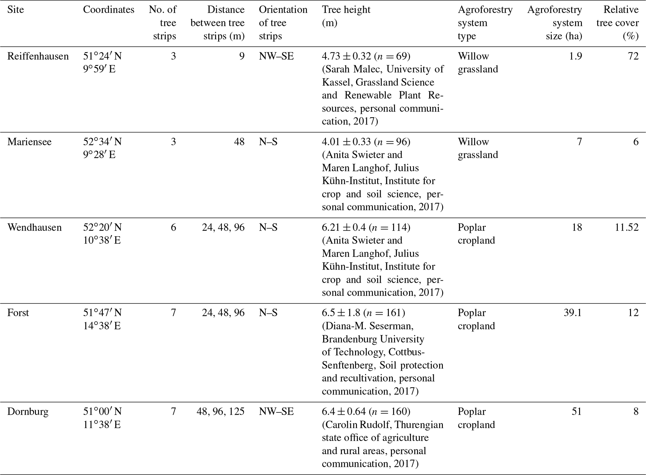
This study was carried out as part of the sustainable intensification of agriculture through agroforestry (SIGNAL) project (http://signal.uni-goettingen.de/, last access: 19 January 2020), to investigate the sustainability of AF systems in Germany. We performed measurements at five sites across northern Germany (Fig. 1, left). Each site consisted of one AF system and one monoculture (MC) system (see Fig. 1 for an aerial photograph of the Dornburg, Forst, Mariensee, Reiffenhausen, and Wendhausen sites with AF and MC selected). The AF systems are of a short rotation alley cropping type, with fast-growing trees interleaved by either crops (see Fig. 1 for images of the cropland AF systems in Dornburg, Forst, and Wendhausen) or perennial grasslands (see Fig. 1 for images of the grassland AF systems in Mariensee and Reiffenhausen). The crops and grasses at the monoculture systems undergo the same tillage and fertilisation as the crops and grasses cultivated between the tree strips. The MC system serves as a reference to the AF system. Table 1 specifies the site locations and the AF geometry.

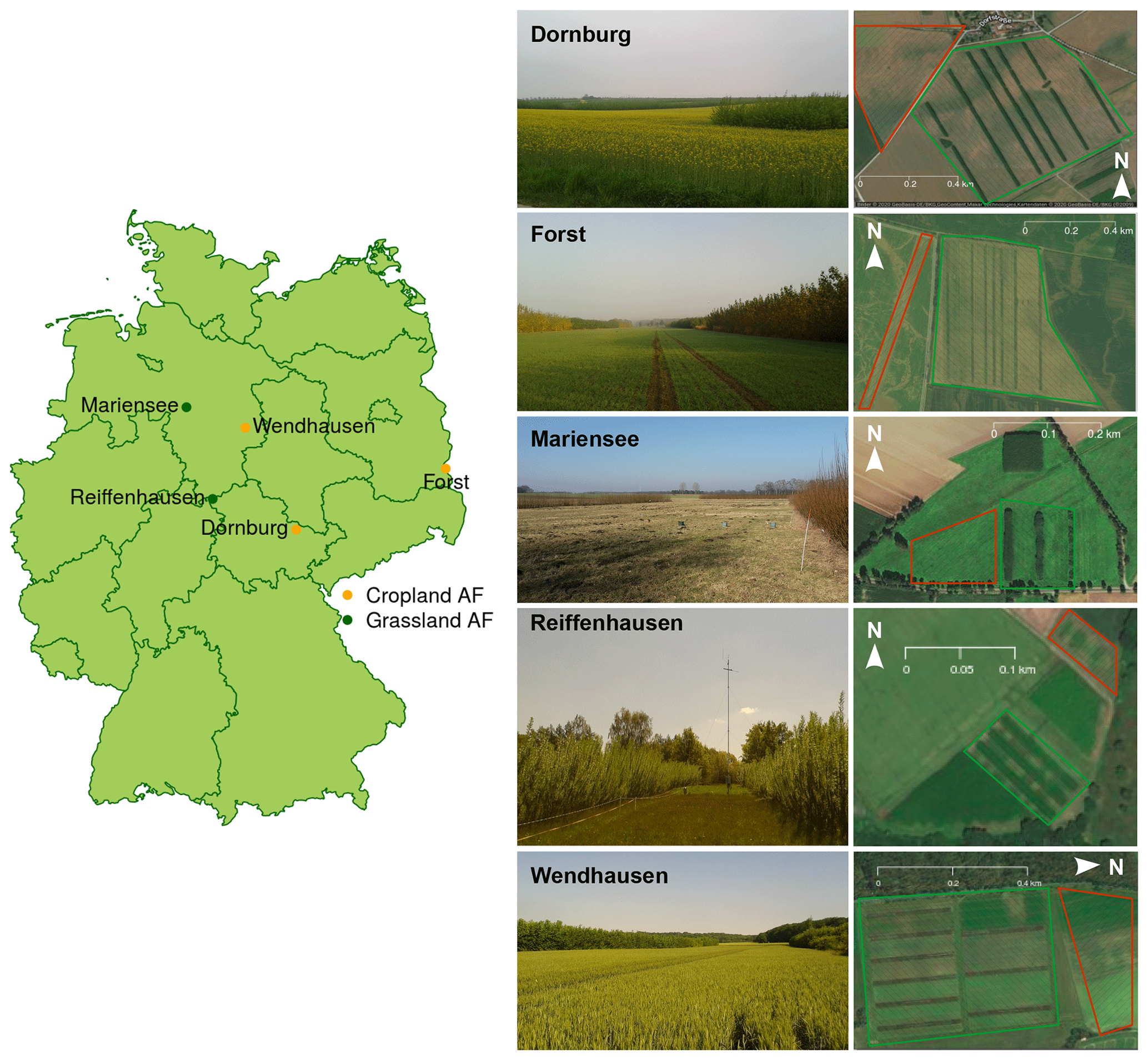
Figure 1 Map of the SIGNAL sites, with the respective agroforestry (AF) system type of either cropland or grassland AF, and an image and aerial photograph of the AF systems. Green hatched areas in the aerial photographs correspond to the area of the AF system, and red hatched areas correspond to the area of the MC system. Site images are our own photographs, and the aerial photographs originate from Google Maps and Google Earth. © Google 2020.

Table 1 Site locations and agroforestry (AF) system geometry.

2.2 Measurements

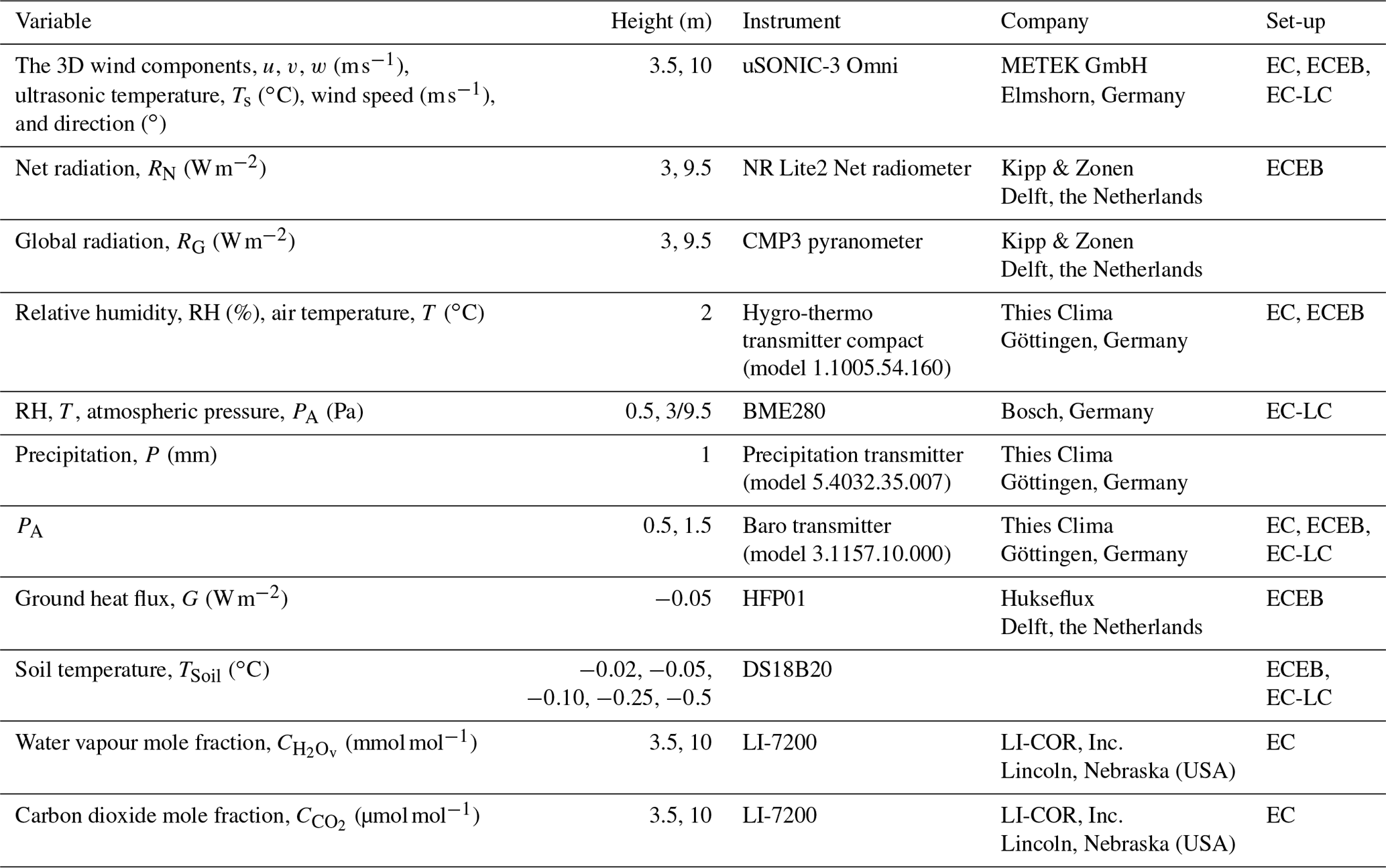
Measurements of meteorological and micrometeorological variables have been performed since March 2016. At each AF system we installed an eddy covariance mast with a height of 10 m, and at each MC system an eddy covariance mast with a height of 3.5 m was installed. Each mast was equipped with the same meteorological and micrometeorological instrumentation. The standard set-up consisted of instruments measuring wind speed, wind direction, sensible heat flux, net radiation, global radiation, air temperature, relative humidity, precipitation, and ground heat flux. An overview of the installed instruments and the respective variables used for the presented set-ups is given in Table 2.

Gaps in precipitation measurements at all sites were filled by precipitation data collected at nearby weather stations operated by the German weather service (DWD). We used the R package of rdwd (Boessenkool, 2019) for data downloads from the ftp server maintained by the DWD. We replaced gaps in precipitation measurements with DWD data if more than 25 % of the precipitation data per day were missing. We used precipitation data from the weather stations at Erfurt–Weimar airport, Cottbus, Hannover–Herrenhausen, and Braunschweig to fill data gaps in precipitation at Dornburg, Forst, Mariensee, and Wendhausen, respectively. In Reiffenhausen we used the precipitation records of a station placed at the same site and operated by the soil hydrology group at the University of Göttingen. As the precipitation transmitter was placed inside or next to the tree strips at the majority of the AF systems, the measurements were affected by interception and were lower than at the MC system. Therefore, we used the precipitation measurements from the MC system to compute ratios of annually summed actual ET and net radiation to precipitation at both AF and MC systems. We assume that the annual sum of precipitation at the AF and the MC systems do not differ due to the relatively small size of the AF systems and no expected local effects of the AF systems on the precipitation formation.

In the following sections, we briefly describe the concepts of the used set-ups, eddy covariance (EC), eddy covariance energy balance (ECEB) and low-cost eddy covariance (EC-LC). Throughout the paper we used the respective abbreviations.

Table 2 Instrumentation for flux and meteorological measurements used at all five AF and MC systems. Set-up corresponds to eddy covariance (EC), low-cost eddy covariance (EC-LC), and eddy covariance energy balance (ECEB).

2.2.1 Eddy covariance (EC)

Sensible heat and momentum fluxes have been measured continuously with ultrasonic anemometers since 2016. The water vapour and CO₂ mole fraction were measured during field campaigns during the vegetation periods of 2016 and 2017 (Table B1). During the field campaigns, the standard set-up was extended by an enclosed-path infrared gas analyser (LI-7200; LI-COR Inc., Lincoln, Nebraska, USA). In 2016, the campaigns were conducted separately at the AF and MC systems with one available gas analyser, whilst in 2017 both systems were sampled simultaneously with two available gas analysers. Data processing and the analysis procedure is described in more detail in Markwitz and Siebicke (2019).

2.2.2 Eddy covariance energy balance (ECEB)

The energy balance at the surface is as follows:

$$\begin{array}{}\text{(1)}& {\displaystyle }{R}_{\mathrm{N}}-G{\displaystyle }=H+\mathrm{LE}+S,\end{array}$$

with net radiation (R_N; W m⁻²), ground heat flux (G; W m⁻²), sensible heat flux (H; W m⁻²), latent heat flux (LE; W m⁻²), and soil storage flux (S; W m⁻²). By convention, a turbulent flux towards the atmosphere is defined as positive and a turbulent flux towards the surface is defined as negative. A positive net radiation corresponds to a surplus of radiative energy at the surface and a positive ground heat flux describes a heat transport into the soil.

LE from ECEB (LE_ECEB) was calculated as the residual of the net radiation, with the ground and sensible heat flux, and the soil storage flux according to Eq. (1) as follows:

$$\begin{array}{}\text{(2)}& {\displaystyle }{\mathrm{LE}}_{\mathrm{ECEB}}{\displaystyle }=R_{\mathrm{N}}-G-H-S,\end{array}$$

assuming a fully closed surface energy balance. The conversion of LE into ET and the derivation of the soil storage flux are given in Sect. A1.

The energy balance residual (Res) per half-hour interval was calculated from Eq. (1) as follows:

$$\begin{array}{}\text{(3)}& {\displaystyle }\mathrm{Res}{\displaystyle }=R_{\mathrm{N}}-\mathrm{LE}-G-H-S,\end{array}$$

with LE from either EC or EC-LC (LE_EC and LE_EC-LC, respectively) and H from EC.

2.2.3 Low-cost eddy covariance (EC-LC)

The EC-LC set-ups comprised the same ultrasonic anemometer uSONIC-3 Omni as used for the EC and ECEB set-ups plus a compact, low-cost relative humidity, air temperature, and pressure sensor (BME280; Bosch, Germany; see Table 2). Water vapour mole fraction was calculated using measurements of relative humidity, air temperature, and air pressure from the low-cost thermohygrometer. A derivation of the water vapour mole fraction from the low-cost thermohygrometer is given in Sect. A2. The turbulent water vapour fluxes were calculated as the covariance between the vertical wind velocity and the water vapour mole fraction from EC-LC, as per the principle of the eddy covariance method (Baldocchi, 2014). The cheaper but slower thermohygrometer had inferior spectral response characteristics compared to a gas analyser with a fast response. The mean spectral correction factor of the thermohygrometer was 42 % larger than for the LI-7200 fast response gas analyser for reference, with a 78 % larger mean time constant of the thermohygrometer compared to the LI-7200. The mean time constant of the thermohygrometer and the LI-7200 was 2.8±1 and 0.6±0.3 s, respectively (Markwitz and Siebicke, 2019). Spectral losses in the high-frequency range of the energy spectrum of the thermohygrometer were corrected by the fully analytical correction method of Moncrieff et al. (1997), which was explicitly recommended for either open-path sensors or closed-path sensors of heated and very short sampling lines. A detailed description and application of the EC-LC set-up for evapotranspiration measurements over AF and MC is given in Markwitz and Siebicke (2019). Evapotranspiration from EC-LC was neither gap-filled for the methodological comparison nor for the analysis of the energy balance closure due to the risk of new errors and artefacts from the respective gap-filling method.

2.3 Gap-filling and energy balance closure adjustment

For the comparison of ET_EC, ET_ECEB, and ET_EC-LC and the estimation of the energy balance closure during the campaigns, we neither gap-filled the data nor corrected the data for the energy balance non-closure. For the calculation of annual sums of ET_ECEB and ET_EC-LC, data gaps were filled and corrected for the energy balance non-closure by distributing the residual equally to H and LE. The residual was estimated by machine learning for times when no data were available. In the following subsections, we describe the gap-filling and energy balance closure adjustment procedures for the ECEB and EC-LC set-ups in more detail.

2.3.1 ECEB

For the calculation of annual sums of ET_ECEB, gaps were filled with the online eddy covariance gap-filling and flux-partitioning tool, REddyProc, developed at the Max Planck Institute for Biogeochemistry in Jena, Germany (https://www.bgc-jena.mpg.de/bgi/index.php/Services/REddyProcWeb, last access: 19 January 2020). The methods used therein are based on Falge et al. (2001) and Reichstein et al. (2005). We corrected ET_ECEB for the average energy balance non-closure, which we estimated from direct LE measurements by EC during measurement campaigns of a minimum of 4 weeks in duration. In the current study we found that considering the energy balance residual reduces ET_ECEB. We used machine learning to estimate the energy balance residuals (Eq. 3) during times when no campaigns took place. We used the machine learning technique of extreme gradient boosting (Chen and Guestrin, 2016; Chen et al., 2019) and predicted the residual energy for both years, 2016 and 2017, at all sites with the R package of XGBoost (Chen et al., 2019).

The calculated residual was treated as the dependent variable, whereas the net radiation, the ground heat flux, and the sensible heat flux were treated as the independent variables. The model was tested with the data gathered during the campaigns and divided into a training period and a testing period. At a ratio of two-thirds of training to testing data, we achieved a Pearson correlation coefficient between the testing and predicted data of 0.66. The trained model was then applied to both years with the net radiation, the ground heat flux, and sensible heat flux as input parameters. As a last step, the predicted residual was subtracted from half-hourly ET. We assumed that the residual distributes equally to the LE and H, and thus we subtracted only half of the residual from ET. Commonly, the residual energy is partitioned according to the Bowen ratio (Twine et al., 2000), which requires direct and continuous measurements of H and LE by EC. We decided on an equal separation of the residual energy because direct LE measurements by EC were not continuously available at our sites. This assumption may cause an overestimation of LE during dry ambient conditions when the Bowen ratio is high. In contrast, LE is expected to be underestimated during moist ambient conditions when the Bowen ratio is small. As no campaign on the energy balance closure was conducted at the monoculture system of Reiffenhausen, we used the data gathered during the campaign at the AF system of Reiffenhausen to train the model and to predict the residual at the MC system.

2.3.2 EC-LC

Unlike for the methodological comparison and energy balance analysis, a gap-filling of ET_EC-LC could not be avoided for the calculation of annual sums of ET. Therefore, for these analyses we gap-filled the half-hourly ET_EC-LC with half-hourly ET_ECEB and corrected both ET_EC-LC and ET_ECEB for the surface energy balance closure as follows:

1. The residual energy was estimated from all available data in 2016 and 2017, following Eq. (3).

2. We trained the same machine learning tool as used for the ECEB set-up to predict the residual energy with the residual treated as the dependent variable and net radiation, ground heat flux, and sensible heat flux the independent variables.

3. The residual was predicted by the trained model; data gaps in the residuals, originating mainly from missing LE caused by data quality checks, were filled with the predicted values.

4. Subsequently, we distributed the residual to ET_EC-LC (${\mathrm{LE}}_{\text{EC-LC}}^{\mathrm{cor}}$) and to ET_ECEB, used for gap-filling (${\mathrm{LE}}_{\mathrm{ECEB}}^{\mathrm{gf}}$) as follows:

   $$\begin{array}{}\text{(4)}& {\displaystyle }& {\displaystyle }\mathit{\alpha }=\mathrm{0.5}\text{(5)}& {\displaystyle }& {\displaystyle }{\mathrm{LE}}_{\mathrm{EC}-\mathrm{LC}}^{\mathrm{cor}}={\mathrm{LE}}_{\mathrm{EC}-\mathrm{LC}}+\mathrm{Res}\cdot \mathit{\alpha }\text{(6)}& {\displaystyle }& {\displaystyle }{\mathrm{LE}}_{\mathrm{ECEB}}^{\mathrm{gf}}={\mathrm{LE}}_{\mathrm{ECEB}}^{\mathrm{gf}}-\mathrm{Res}\cdot \mathit{\alpha }.\end{array}$$

2.4 Energy balance closure estimation

The energy balance closure (EBC) was quantified in two ways:

1. First, as the linear regression between the sum of the turbulent flux components (LE+H) and the available energy ($R_{\mathrm{N}}-G-S$). We applied the major axis linear regression (Webster, 1997), which assumes equally distributed errors in both time series. We interpreted the slope between the sum of the turbulent fluxes and the available energy as the closure of the surface energy balance. A slope of one and an intercept of zero corresponds to perfect energy balance closure. In the present study, both the slope and the intercept were considered as variable.

2. Second, as the energy balance ratio (EBR), also called the “instantaneous energy balance closure” (Stoy et al., 2013). Thus, the closure per half-hour is as follows:

   $$\begin{array}{}\text{(7)}& {\displaystyle }\mathrm{EBR}{\displaystyle }={\displaystyle \frac{\mathrm{LE}+H}{R_{\mathrm{N}}-G-S}},\end{array}$$

with either LE_EC or LE_EC-LC.

2.5 Flux footprint analysis

The spatial coverage and the position of the source area of turbulent sensible and latent heat fluxes and momentum at a specific point in time is defined by the flux footprint (Schmid, 2002; Kljun et al., 2015). In the present study, a flux footprint climatology was calculated with the flux footprint prediction online data-processing tool developed by Kljun et al. (2015) (http://footprint.kljun.net/, last access: 19 January 2020). The analyses were performed separately for the respective campaign periods (see Table B1 in Appendix B for dates) and for both years at each site. We selected only daytime data, according to a global radiation R_G > 20 W m⁻².

2.6 Canopy resistance

The effects of structural differences between AF and MC on ET were studied in terms of the relationship between half-hourly ET and the aerodynamic and canopy resistances (s m⁻¹). The canopy resistance was calculated from the rearranged Penman–Monteith equation (see Eq. A12 in Appendix A3) for evapotranspiration, which depends on the canopy resistance ($r_{\mathrm{c}}=\mathrm{1}/g_{\mathrm{c}}$; s m⁻¹) and the aerodynamic resistance for heat ($r_{\mathrm{ah}}=\mathrm{1}/g_{\mathrm{ah}}$; s m⁻¹). The canopy resistance follows the big leaf assumption, which assumes that the whole canopy response to environmental changes equals the response of a single leaf. This assumption is valid for the monoculture system with a single crop type of similar height. For the AF systems, this assumption might be violated due to the heterogeneity of the AF systems with different plant species (trees and crops) of different heights. In the lee of the tree strips, the reduced wind speed and incident radiation might lead to reduced ET due to a different leaf stomata regulation of sunlit and shaded leaves. In the windward site of the tree strips, trees and crops are affected by increased wind velocities and varying incident radiation; thus, the opposite conditions, compared to the lee of the tree strips, are found. However, we assume that the meteorological data from the flux tower represent the mean state of the meteorological conditions within the AF system. Therefore, we are confident that the big leaf assumption also holds for AF systems.

We studied the relationship between ET and canopy resistance and aerodynamic resistance for idealised ambient conditions with global radiation (R_G≥400 W m⁻²), horizontal wind speed (u≥1 m s⁻¹), and vapour pressure deficit ($D=\mathrm{1}\pm \mathrm{0.3}$ kPa; Schmidt-Walter et al., 2014). A derivation of the canopy resistance is given in Sect. A3.

3 Results and discussion

3.1 Meteorological conditions during the campaigns

For the meteorological conditions during the campaigns, we refer to the time series of the relevant meteorological parameter in Fig. 2 and mean values in Table 3.

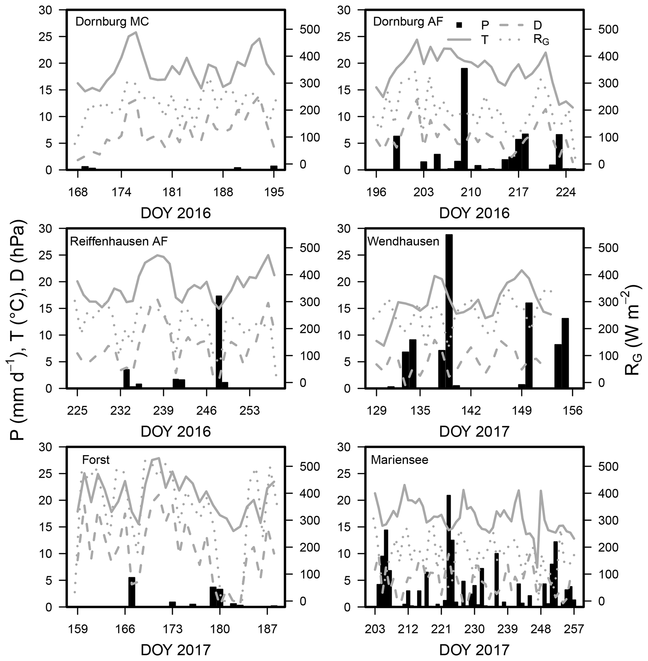
Figure 2 Time series of daily mean air temperature (T; ^∘C), vapour pressure deficit (D; hPa), daily summed precipitation (mm d⁻¹; left y axis), and daily mean global radiation (R_G; W m⁻²; right y axis) for all sites. The data for AF and MC of the respective sites of Forst, Mariensee, and Wendhausen were averaged. The field campaigns at the AF and MC systems were conducted during the same time, and we assumed similar weather conditions due to the small distance between the AF and MC system.

Table 3 Mean air temperature (T; ^∘C), vapour pressure deficit (D; hPa), global radiation (R_G; W m⁻²), and the cumulative precipitation (P; mm d⁻¹) for the respective site and campaign period. Data for Reiffenhausen MC are missing due to the unavailability of a campaign.

3.2 Flux footprint climatology

The flux footprint analyses showed that the measured turbulent fluxes were representative of the larger AF systems and their respective MC systems during the time of the experiments (e.g. Dornburg, Forst and Wendhausen, Fig. 3). At the AF and MC systems of Dornburg, 80 % of the flux magnitude originated from the respective system. The 90 % flux magnitude contribution line at the AF system overlapped with the 90 % flux magnitude contribution line at the MC system to the west. The overlapping footprint was also found for the annual footprint analyses (see Fig. C3 in Appendix C).

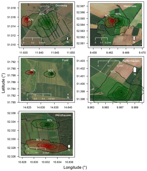
Figure 3 Flux footprint climatologies for all sites for the respective campaign period. Green shaded footprints correspond to the AF system, and red shaded footprints correspond to the MC system. For the analysis only daytime data were used (R_G>20 W m⁻²). Isolines correspond to a 10 % to 90 % flux magnitude contribution in 10 % steps, with the 90 % isoline labelled in the system. The flux footprint climatology for Reiffenhausen MC is missing due to the unavailability of a campaign. Aerial photographs originate from Google Maps and Google Earth. © Google 2020.

At the AF and the MC system of Wendhausen, we observed a 80 % flux magnitude contribution from both land uses to the total turbulent flux (Fig. 3). A 10 % flux magnitude contribution originated from the forest around 200 m east of the flux tower. Easterly winds are most likely during stable atmospheric stratification in winter or summer. During the time of the experiment, the wind mainly originated from a westerly direction (not shown).

A total of 70 % of the area of the AF and MC grassland systems of Mariensee contributed to the measured fluxes, respectively (Fig. 3). The remaining 20 % of the area contributing to the measured flux originated from surrounding crops and the AF and MC grassland systems. There was an overlap of the two footprints at the AF and the MC grassland system, which was expected as both flux towers are separated by a distance of about 200 m.

The fluxes measured at the smallest AF system in Reiffenhausen were influenced by fluxes originating from the nearby forests and crop fields at about a 400 m distance from the flux tower in a northerly direction and about 200 m distance in a southerly direction (Fig. 3). Only 60 % of the fluxes originated from the willow–grassland AF system and the short rotation willow plantation in the west. The terrain at the AF system of Reiffenhausen is sloped towards the northwest. The main wind direction at the site was north-northwest in the direction of the sloped terrain.

3.3 Diel evapotranspiration

The diel variation of ET for all three set-ups at all sites is depicted in time series plots for an exemplary time period in Fig. 4.

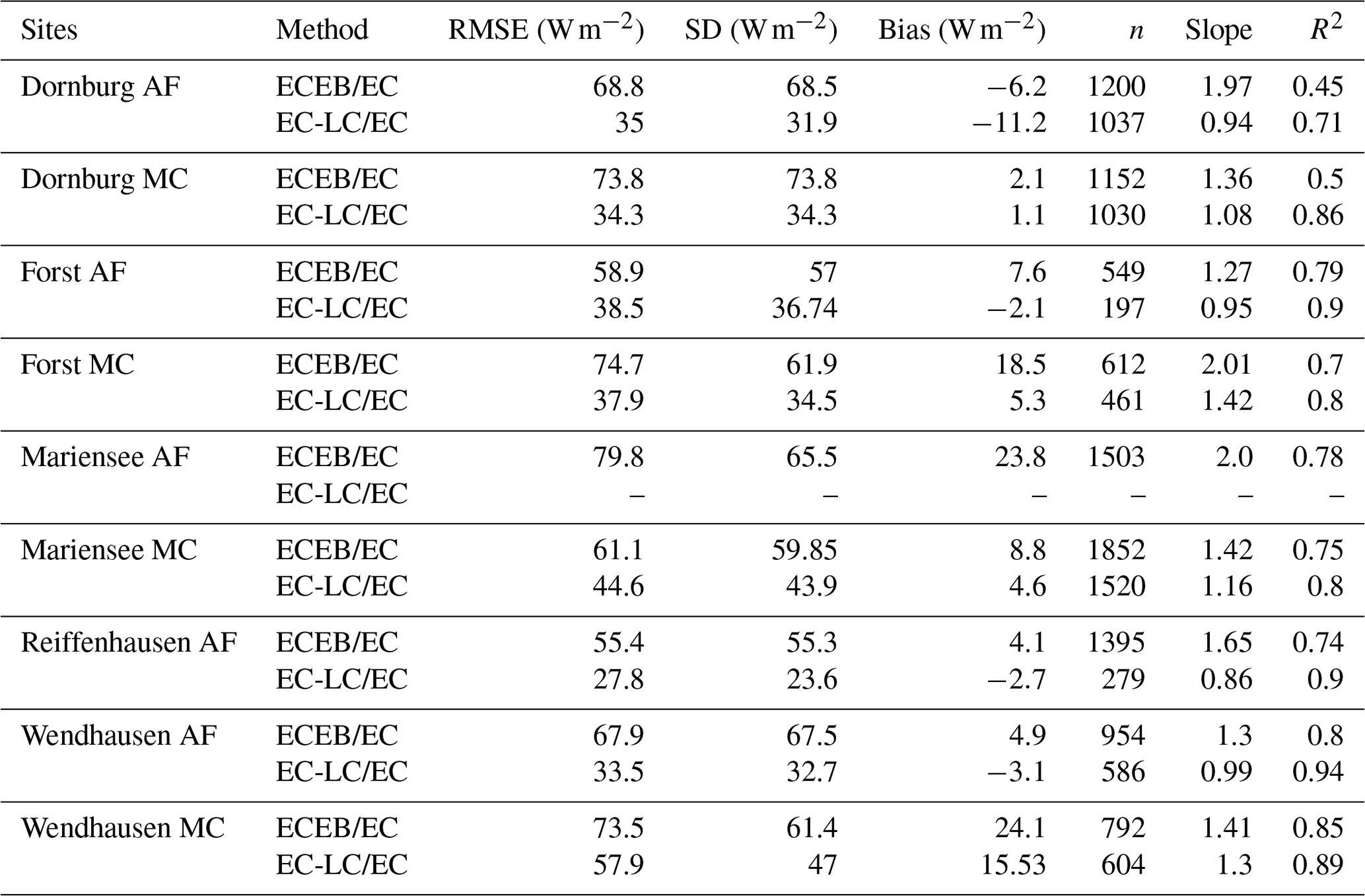
The EC-LC set-up showed the best performance relative to direct EC measurements, with coefficients of determination between a minimum of 71 % and a maximum of 94 %. The EC-LC set-up captured the temporal variability of ET and the flux response to changing ambient conditions as well as the direct EC measurements. The slopes from a linear regression analysis of LE_EC-LC vs. LE_EC showed an agreement between 86 % and 99 % across four AF systems and between 108 % and 142 % across four monoculture agriculture systems (see Table 4 and Fig. C2).

At the MC systems of Forst and Wendhausen (Fig. 4), we observed comparably high ET_EC-LC relative to direct EC measurements, while attaining high coefficients of determination. We suspect that the laser source of the LI-7200 gas analyser did not work as expected as indicated by the spectral analysis (data not shown). Only low-frequency fluctuations were sampled, whereas the high-frequency fluctuations were attenuated. The spectral response characteristics of the gas analyser and the thermohygrometer set-up were similar. Therefore, the correction of high-frequency losses is expected to be higher for the compromised gas analyser at the respective MC systems than for a fully functional gas analyser.

ET_ECEB also captured the diel cycle of ET and gave an indication of the ecosystem response to changing meteorological drivers (Fig. 4). ET_ECEB overestimated ET_EC across all sites. A minimum overestimation of 27 % was observed at the AF system of Forst, and a maximum overestimation of 101 % was observed at the MC system of Forst at a half-hourly timescale (see Table 4 and Fig. C1). Differences between ET_ECEB and ET_EC were attributed to the assumption of a fully closed energy balance at the surface (Foken et al., 2006). ET_ECEB was calculated as the residual of net radiation, sensible heat flux, ground heat flux, and soil storage. In this analysis, we did not account for the commonly observed non-closure of the energy balance and added the surface energy balance residual completely to LE.

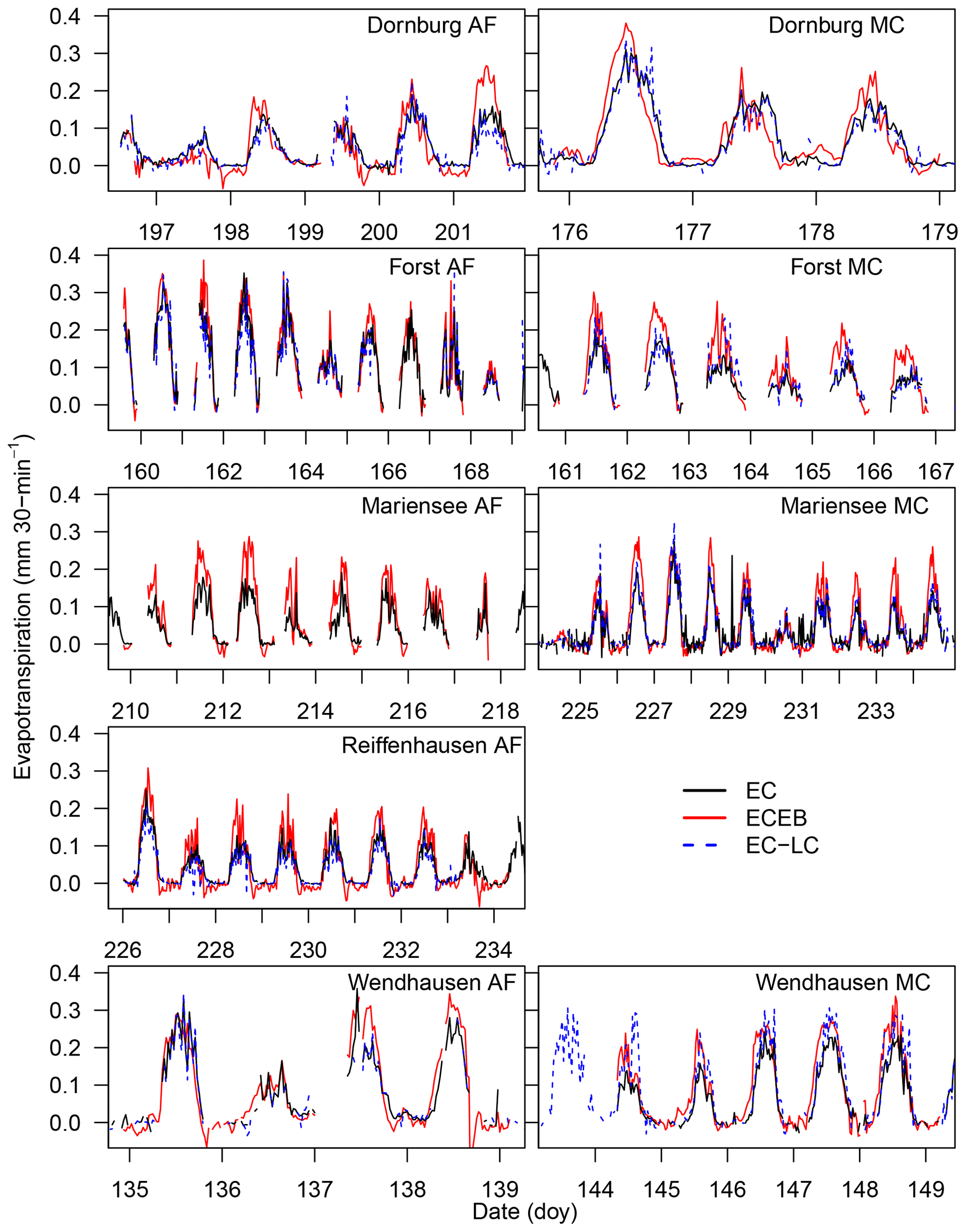
Figure 4 Time series of half-hourly evapotranspiration rates of an exemplary time period for ECEB, EC-LC, and EC as a reference for all sites. Time series of half-hourly ET rates for Reiffenhausen MC are missing due to the unavailability of a campaign, and ET_EC-LC at Mariensee AF are missing due to technical problems with the sensor during the campaign. The presented time series were not corrected for the energy balance non-closure. Gaps in nocturnal data are due to the limited power availability from the solar power supply.

Table 4 Statistical analysis results for a linear regression of LE_EC-LC vs. LE_EC and LE_ECEB vs. LE_EC. Shown here are the root mean square error (RMSE), the standard deviation of the differences between both set-ups (SD), the bias (Bias), the number of points used for the analysis (n), the slope for a linear regression of LE_EC-LC vs. LE_EC and LE_ECEB vs. LE_EC, and the coefficient of determination of the linear regression (R²). Data for LE_EC-LC at Mariensee AF are missing due to technical problems with the sensor during the campaign, and data for Reiffenhausen MC are missing due to the unavailability of a campaign.

3.4 Energy balance closure (EBC)

3.4.1 EBC from EC and EC-LC

The mean EBC was 79.4±8.5 % and 79.25±6 % across the five AF systems and four MC systems for LE_EC (see Fig. 5 and Table 5). The coefficient of determination, R², was a minimum of 0.77 and a maximum of 0.92 across sites (Table 5).

The EBC for LE_EC at the AF and the MC systems were comparable to agricultural systems as reported by Stoy et al. (2013), who found a mean EBC of 84±20 % across 173 FLUXNET sites, a mean EBC of 91 % to 94 % for evergreen broadleaf forests and savannas, and a mean EBC of 70 % to 78 % for crops, deciduous broadleaf forests, mixed forests, and wetlands. Imukova et al. (2016) found an EBC of 71 % and 64 % for two consecutive growing seasons over a winter wheat stand in Germany. Studying a belt and alley system in Australia, Ward et al. (2012) found an EBC between 67 % and 80 % over the time period of 6 months. Fischer et al. (2018) reported on the water requirements of three short rotation poplar stands and found a mean long-term energy balance closure of 82 % at a site in Italy, an EBC of 91 % or 95 % at a site in the Czech Republic, and an EBC of 69 % at a site in Belgium.

The EBC for LE_EC-LC was slightly lower at the AF systems with a mean EBC of 79±5.3 % compared to the MC systems with a mean EBC of 82±11.8 % for five sites. The differentiation into lower EBC at the AF and higher EBC at MC systems observed for the two different set-ups is in agreement with the linear regression results presented in Sect. 3.3. At the AF systems, LE_EC-LC was lower than LE_EC. In the calculation of the energy balance closure only LE was changed, and the other energy balance components were held constant. Therefore, increased LE led to a decreased residual energy and, subsequently, to a better fit of the energy balance closure.

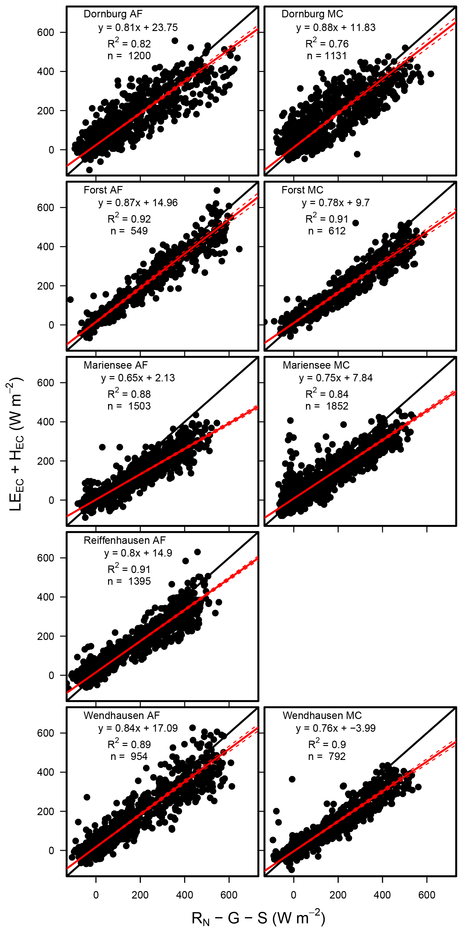
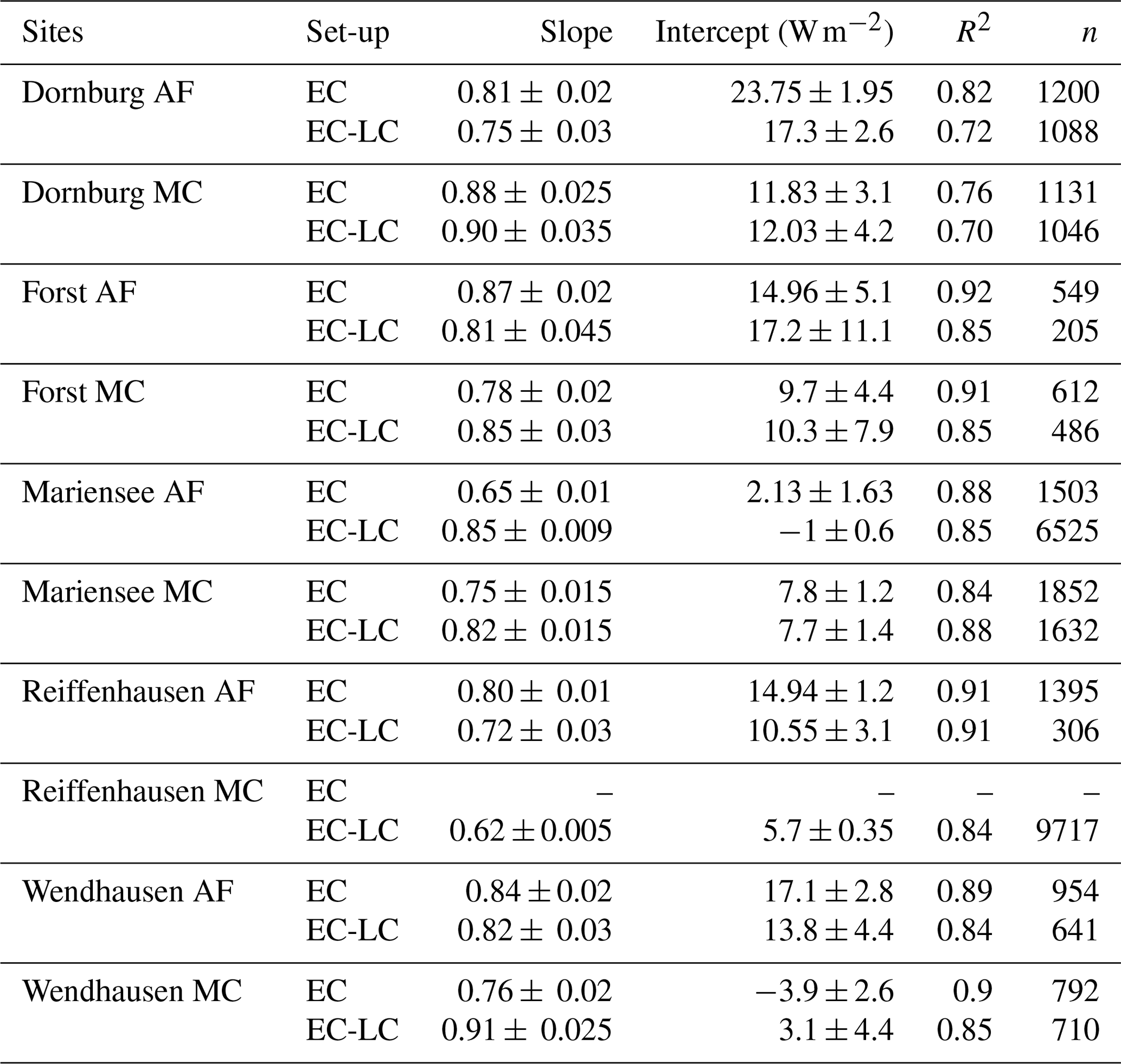
Figure 5 Scatterplot of the sum of the turbulent fluxes (LE_EC+H_EC) vs. the sum of the available energy ($R_{\mathrm{N}}-G-S$) for all sites. Each plot contains the linear regression equation, the coefficient of determination (R²), and the number of data points used for the analysis (n). Data for Reiffenhausen MC are missing due to the unavailability of a campaign.

Table 5 Statistical analysis results of the linear regression between the sum of the turbulent fluxes and the available energy, namely the sites, the set-up used, the slope (±5 % confidence interval), the intercept, the coefficient of determination of the linear regression (R²), and the number of points used for the analysis (n). The energy balance closure determined by EC-LC at Mariensee AF is based on data collected from 23 March to 20 November 2016, and at Reiffenhausen MC, the analyses are based on data collected from 7 April to 31 December 2016 due to the unavailability of data during the campaigns. The energy balance closure determined by EC for Reiffenhausen MC is missing due to the unavailability of a campaign.

3.4.2 Diel cycles of the energy balance ratio and the energy balance residual

The diel cycle of the energy balance ratio from LE_EC at the sites can be classified into two different patterns. The diel cycle of the EBR for Dornburg (Fig 6) shows a strong increase between 06:00 and 08:00 local time (LT), followed by a positive slope between 08:00 and 14:00, and a strong increase thereafter until 18:00. The EBR is a minimum of 0 at 06:00 and a maximum of 1.8 at 18:00. The diel cycle of the EBR at the remaining sites (Forst, Mariensee, Reiffenhausen, and Wendhausen; Fig. 6) is the lowest at 06:00 and 18:00 with an EBR of 0.5, whereas between 08:00 and 16:00 the EBR is fairly constant and at a similar range as the EBC estimated for all sites and the whole campaign (Table 5).

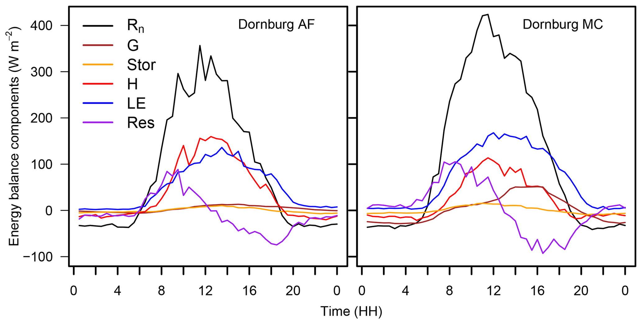
The Dornburg site might be affected by the horizontal advection of moisture and heat. Oncley et al. (2007) reported that the advection of moisture had the highest contribution to the unclosed energy balance compared to the other components. The maximum peak of the horizontal moisture advection term was in the afternoon, as energy was accumulated during the day and released in the afternoon. We suspect that this is also the case for the Dornburg site. The sensible heat flux follows the diurnal cycle of available energy, with the maximum peak at midday at the agroforestry and the monoculture system (Fig. 7). In contrast, the median of the latent heat flux had its maximum in the afternoon at around 14:00 and was positive even after the available energy changed its sign.

In addition to advective transport, the unclosed surface energy balance could be related to energy storage terms such as biomass, the air, or photosynthesis (Jacobs et al., 2008), which have not been considered previously. The pattern seen at Dornburg may be attributed to a release of energy during the afternoon, which corresponds to a surplus of energy and a better closure of the energy balance. In the morning hours, the storage terms have an opposite sign, which corresponds to a lack of energy and a subsequent poorer energy balance closure. Considering the storage terms would lead to a reduction in the residual energy and a better closure of the energy balance.

Interestingly, the diel pattern of the EBR from LE_EC at both land uses at all sites are equal. Additionally, the differences between the median diel cycle EBRs (between 06:00 and 18:00) at the AF and the MC system were small, with differences of a minimum of −0.09 and a maximum of 0.13 across sites. As both flux towers located at the AF and the MC system at one site are separated by approximately 100 to 500 m and the diel patterns look similar, we suspect that the non-closed surface energy balance at one site is caused by local effects of a longer wavelength than the commonly applied averaging period of 30 min and is thus beyond the individual site level.

The diel cycles of the EBRs and the residuals were similar for both EC-LC and EC set-ups (Fig. C4). This is promising, as it indicates, first, a performance of EC-LC comparable to EC, and, second, the capability of the EC-LC set-up to capture site-specific effects. Nevertheless, the observed differences between EBRs and residuals at the AF and MC at one site were mostly attributed to differences in LE. Higher LE_EC-LC than LE_EC led to higher EBRs.

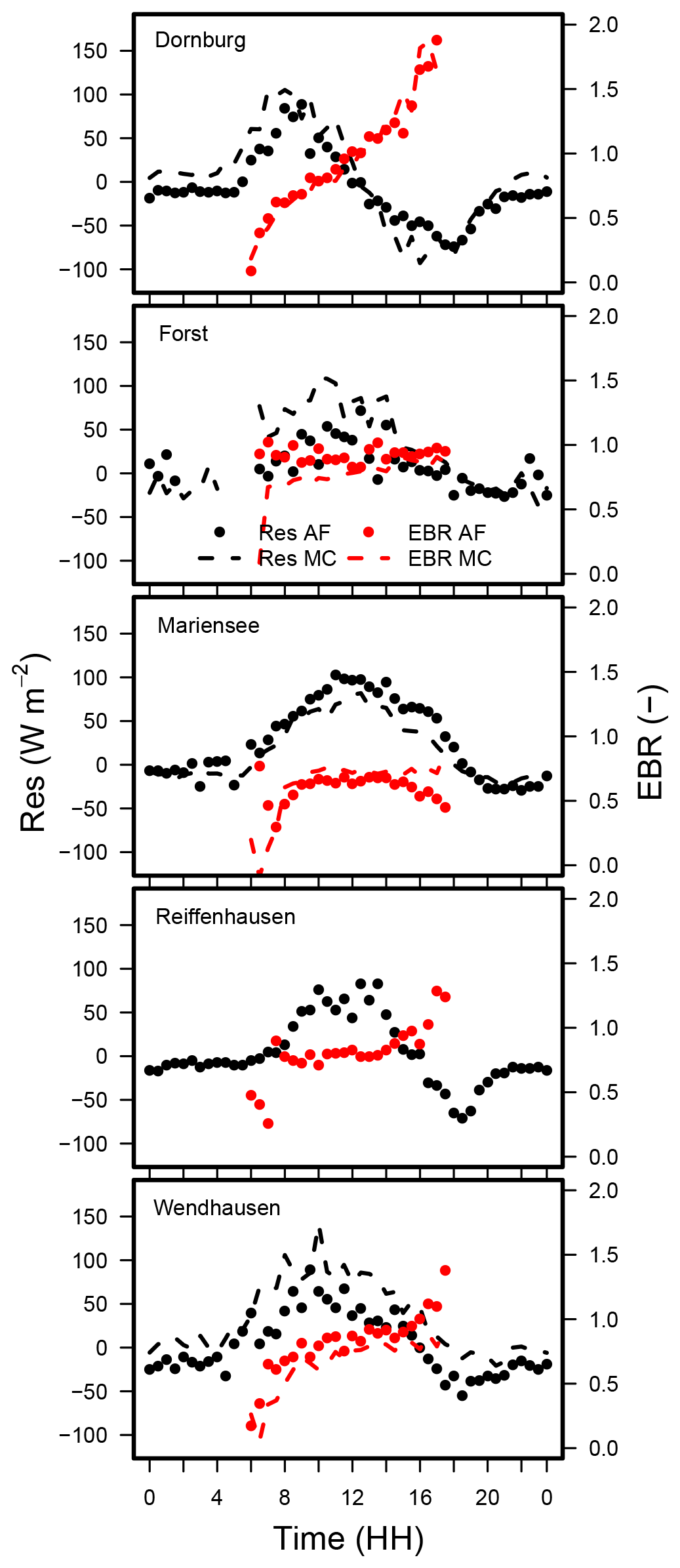
Figure 6 Median diel cycle of the energy balance ratio (EBR) and diurnal cycle of the residual energy for the AF and the MC systems at all sites. LE and H were obtained by EC. Data from Reiffenhausen MC are missing due to the unavailability of a campaign.

Figure 7 Median diurnal cycle of the energy balance components for Dornburg AF and MC for the campaign times (see Table B1).

3.5 Evapotranspiration over agroforestry

3.5.1 Sums of evapotranspiration during the campaigns

Sums of evapotranspiration for all three methods, all sites, and campaign periods indicate higher sums of ET_ECEB relative to ET_EC, except for Dornburg AF (Fig. 8). The difference between sums of ET_ECEB and ET_EC reflects the unaccounted correction of ET_EC and ET_ECEB for the energy balance non-closure. The large difference between sums of ET_ECEB and ET_EC at Mariensee AF correspond to the low energy balance closure of 65 % at the site. Differences between sums of ET_EC-LC and ET_EC correspond to lower ET_EC-LC than ET_EC over the AF systems and higher ET_EC-LC than ET_EC over the MC systems. This is indicated by slopes smaller and higher than one of a linear regression analysis between ET_EC-LC and ET_EC (Table 4).

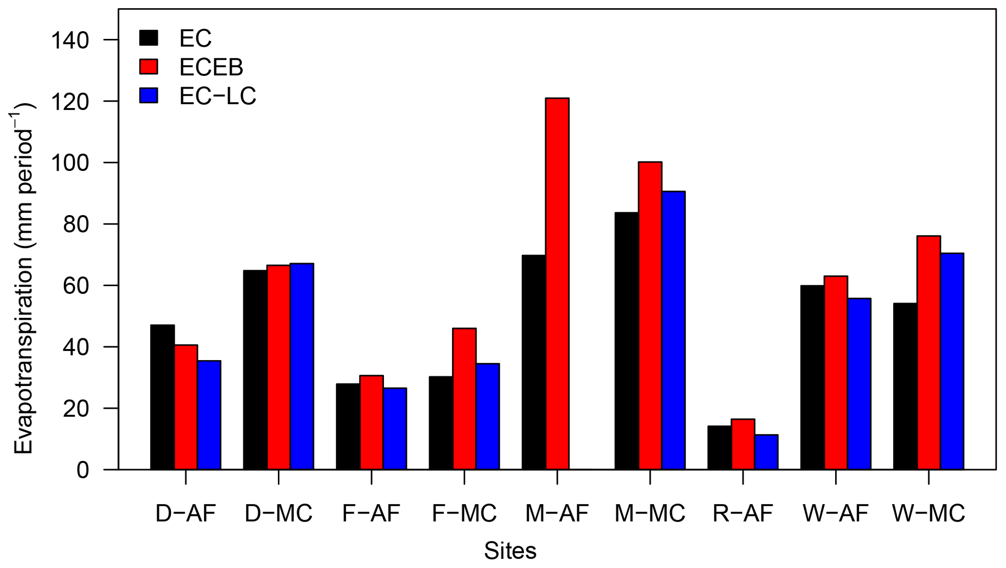
Figure 8 Sums of uncorrected and not gap-filled half-hourly evapotranspiration for all three methods and all sites during the campaign periods. Sites are abbreviated by their first letter and are identified as being either AF (agroforestry) or MC (monoculture). Incomplete records with ET_EC, ET_ECEB, or ET_EC-LC missing were omitted. Data for ET_EC-LC at Mariensee AF are missing due to technical problems with the sensor during the campaign, and all data for Reiffenhausen MC are missing due to the unavailability of a campaign.

3.5.2 Weekly sums of evapotranspiration

The annual cycle of evapotranspiration across all sites and for the years 2016 and 2017 depicts the typical seasonal cycle of the highest ET during summer and the lowest ET during winter (Fig. 9). We found small differences between the weekly sums of ET at the AF and the MC systems during the main growing period of the crops. After the ripening of the crops, we found higher weekly sums of ET at the AF systems compared to the MC systems at the cropland sites of Dornburg, Forst, and Wendhausen (Fig. 9). We assume that, after the ripening of the crops, evaporation contributed the most to the measured ET at the MC system, whereas at the AF system both evaporation from the crop fields between the tree strips and transpiration from the trees contributed to the measured flux. At the grassland sites of Mariensee and Reiffenhausen (Fig. 9), differences in the weekly sums of ET between both land uses were small, with a tendency towards higher ET rates at the MC system compared to the AF system.

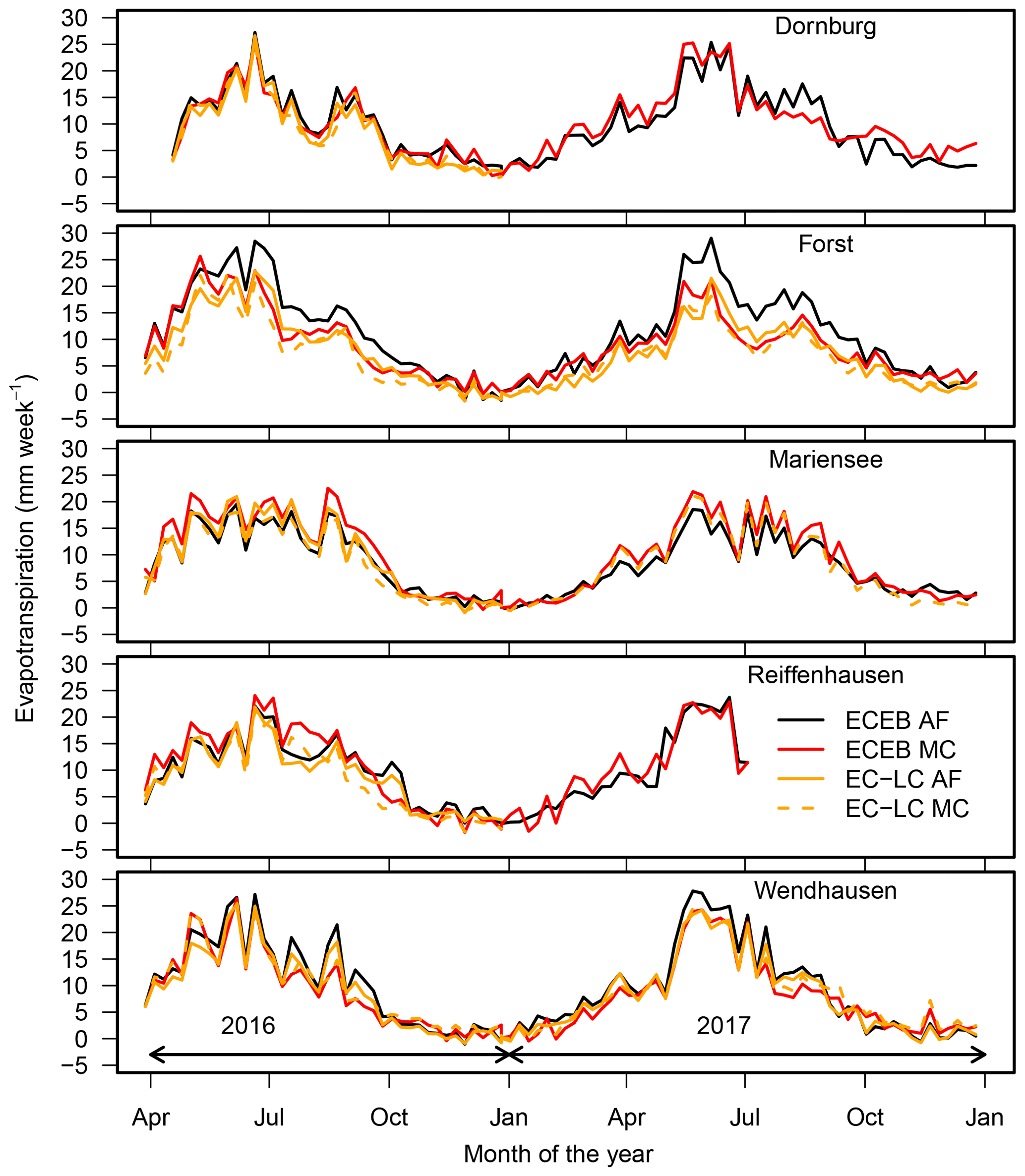
Figure 9 Weekly sum of half-hourly ET_ECEB (black and red solid lines for AF and MC, respectively) and ET_EC-LC (orange solid and dashed lines for AF and MC, respectively) for all sites. In 2017, data in Reiffenhausen AF and MC were only available until the end of July due to station failure.

3.5.3 Annual sums of evapotranspiration

Differences between the annual sums of ET for the two land uses, AF and MC, were in the range of a maximum of +31 % and a minimum of −16 % (see Fig. 10 and Table 6) across sites and methods. We wanted to understand where differences between annual sums of ET come from. Therefore, we investigated differences between ET according to (1) the effect of the different land uses, i.e. AF and MC, (2) the effect of different methods, i.e. EC-LC and ECEB, and (3) the effect of different years, i.e. 2016 and 2017, with different precipitation inputs.

For this purpose, we used the relationship between the evapotranspiration index ($\sum \mathrm{ET}/\sum P$) and the radiative dryness index (R_N∕λP) proposed by Budyko (Budyko, 1974). Figure 11a shows the ET index as a function of the radiative dryness index for all sites, both set-ups, and both years.

The figure indicates, first, that plots with an ET index larger than one were water limited, corresponding to an radiative dryness index $R_{\mathrm{N}}/\mathit{\lambda }P>\mathrm{1}$. Second, the figure shows a separation between the sites with an energy limitation ($R_{\mathrm{N}}/\mathit{\lambda }P<\mathrm{1}$) and water limitation ($R_{\mathrm{N}}/\mathit{\lambda }P>\mathrm{1}$) for the years 2016 and 2017, respectively.

With regards to the first finding, in 2016 the grassland site of Mariensee MC and Reiffenhausen AF and MC had an ET index larger than one. At those sites, the annual sum of ET was generally high relative to the annual sum of precipitation (Fig. C5a). This finding seems to be typical for grasslands. Williams et al. (2012) reported that there was on average a 9 % higher transformation of precipitation into evapotranspiration at grasslands compared to forests across 167 sites as part of FLUXNET, the global flux measurement network. They concluded, first, that higher ET of grasslands may have been caused by the less conservative water use compared to trees, and second, that it could indicate that grasses have an extensive, well-developed root system similar to trees. Nevertheless, considering the water balance equation with precipitation equalling the sum of evapotranspiration and water runoff, an ET index larger than one indicates water losses via ET and no runoff. An ET index larger than one is only to be expected under groundwater access, irrigation, or the impact of a nearby stream. At the grassland site of Mariensee it is likely that the trees and grasses had groundwater access, as the groundwater table was at about a 1.5–2 m depth.

The AF system in Reiffenhausen is located on a gentle slope with no groundwater access, which we expect should promote run-off, contrary to the high ET index observed. But the ET measurements are affected by a poplar and willow SRC in the south-southeast and north-northwest directly within the flux footprint (see Sect. 3.2 and Fig. 3). And with respect to the overall area of the AF system, the area covered by trees amounts to 72 % and is much higher compared to the other sites (Table 1). In both cases, a radiative dryness index larger than one is also possible, despite this indicating a water limitation at the particular sites. Additionally this also indicates a surplus of radiative energy, which promotes photosynthesis and higher transpiration, assuming that soil water is not limited. In contrast, the Mariensee and Wendhausen sites had evapotranspiration and radiative dryness indices of approximately 0.5 and 0.6 in 2017. Those sites were affected by exceptionally high annual precipitation events, but annual sums of ET were comparable to 2016 (Table 6).

The second finding gives evidence of a dependency of ET on the local climate. The years 2016 and 2017 correspond to a dry and a wet year, respectively. In Fig. 11a and b, arrows indicate the difference between mean evapotranspiration indices and mean radiative dryness indices grouped by year, method, and land use. The length of the arrows corresponds to the overall difference. The ET index averaged over all annual sums of ET for the years 2016, and 2017 showed the largest difference, with a trend from a water-limited (2016) regime to an energy-limited (2017) regime. Higher available energy and lower precipitation than normal in 2016 led to a higher radiative dryness index, whereas lower available energy and higher precipitation led to a smaller radiative dryness index in 2017. Differences between mean ET indices from the two methods had the second largest impact on annual sums, with a trend of a higher mean ET index of ET_ECEB compared to ET_EC-LC. The land use type had the least impact on differences between the ET indices, with a small trend of higher ET∕P over AF than over MC.

However, our results indicate that the effect of agroforestry on ET is small compared to differences between methods and differences between years with different precipitation regimes. We therefore reject the initial hypothesis that short rotation alley cropping agroforestry systems lead to higher water losses to the atmosphere via ET, compared to monoculture agriculture without trees.

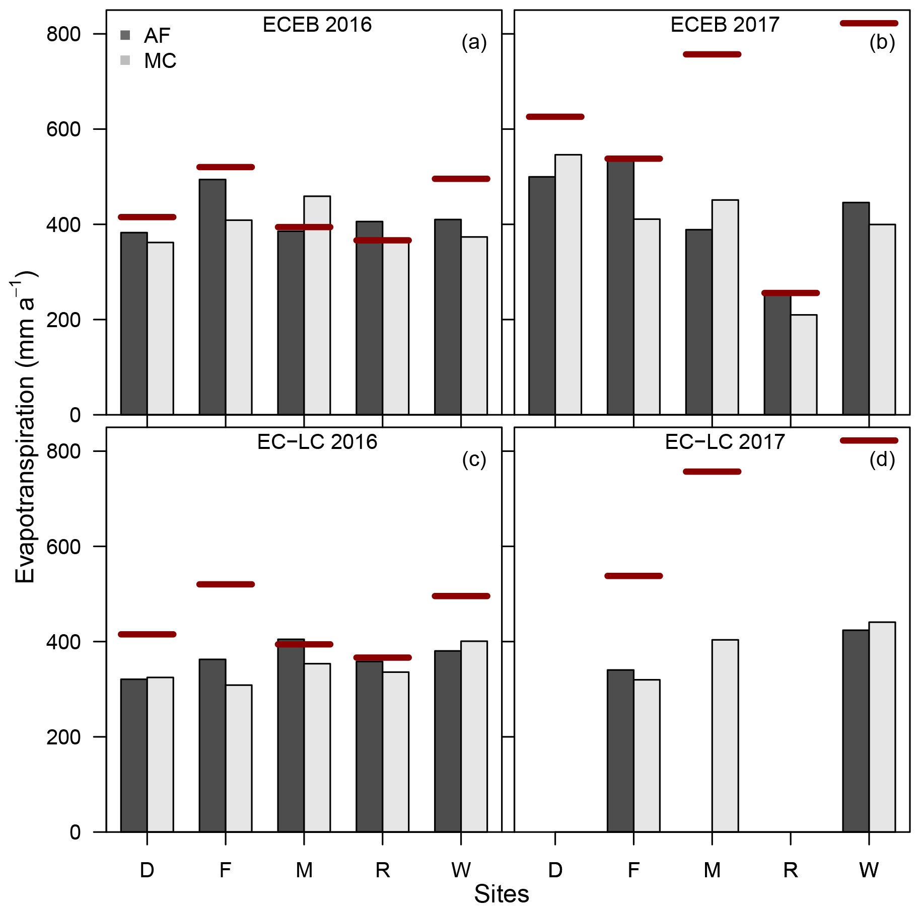
Figure 10 Annual sums of ET_ECEB in 2016 (a) and 2017 (b) and ET_EC-LC in 2016 (c) and 2017 (d) for Dornburg (D), Forst (F), Mariensee (M), Reiffenhausen (R), and Wendhausen (W). The red solid lines correspond to the annual sum of precipitation from the monoculture system of the respective site. The annual sums of evapotranspiration at Reiffenhausen AF and Reiffenhausen MC in 2017 contain only data from 1 January to 9 July 2017 due to station failure. Annual sums of ET_EC-LC for Dornburg AF and MC, Mariensee AF, and Reiffenhausen AF and MC in 2017 are missing due to instrument malfunctions.

Table 6 Annual sums of energy balance closure corrected actual evapotranspiration, ET (mm a⁻¹), and precipitation, P (mm a⁻¹) for all sites, both set-ups (ECEB and EC-LC), and both years (April to December 2016; January to December 2017). The annual sums of ET_ECEB and precipitation at Reiffenhausen AF and MC in 2017 contain data from 1 January to 1 July 2017 due to the destruction of the station. Annual sums of ET_EC-LC for Dornburg AF and MC, Mariensee AF, and Reiffenhausen AF and MC in 2017 are missing due to instrument malfunctions.

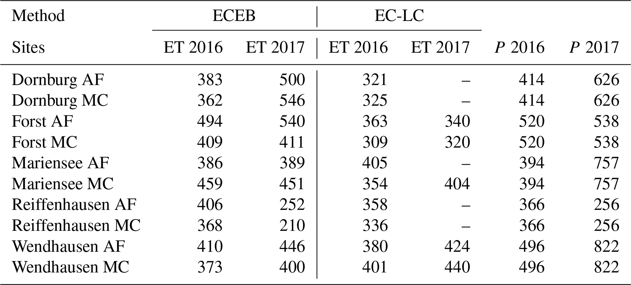
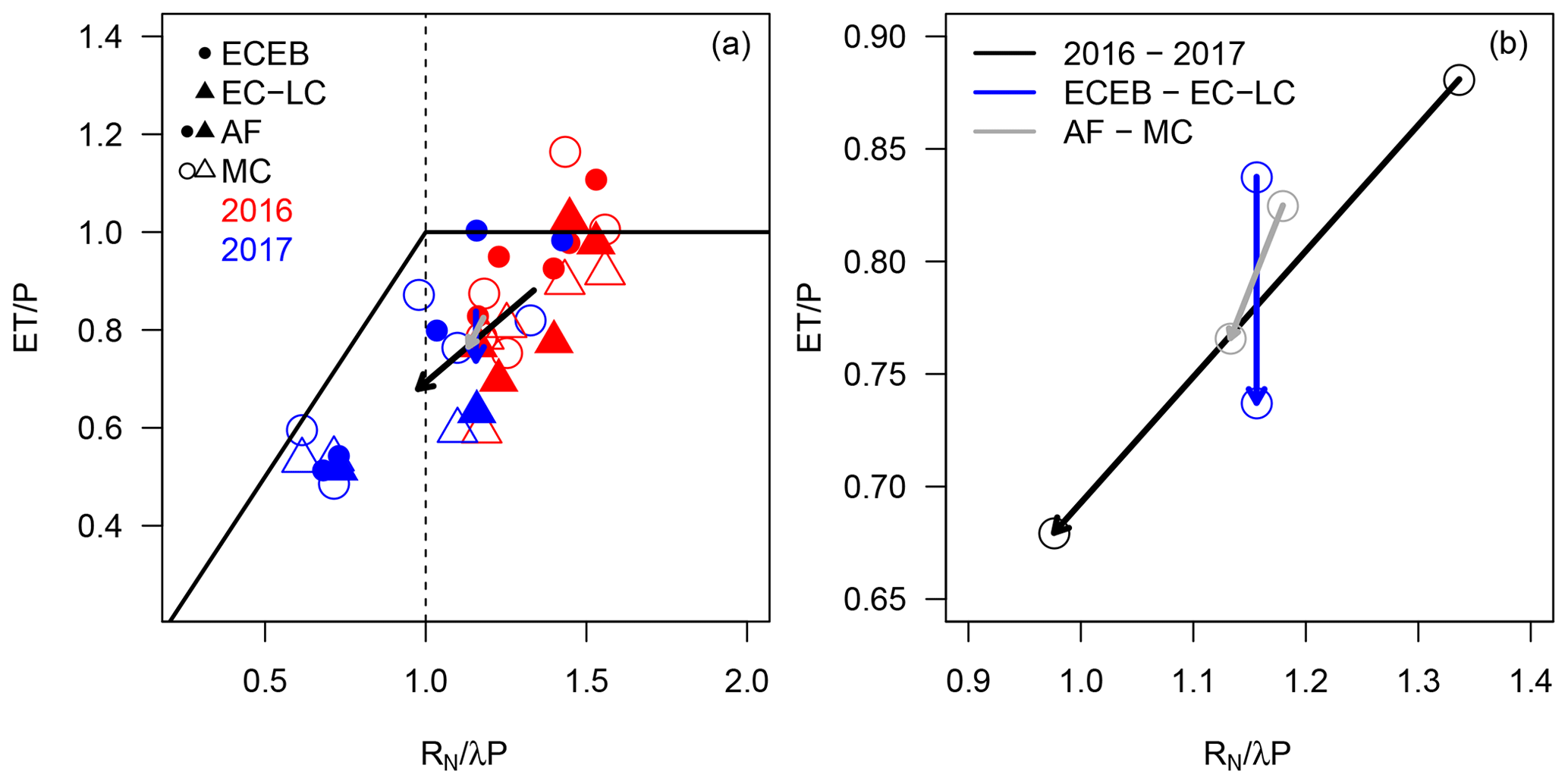
Figure 11 (a) Evapotranspiration index (ET∕P) vs. the radiative dryness index (R_N∕λP) for both land uses (AF – filled triangles and dots; MC – empty triangles and dots), both set-ups (ECEB – dots; EC-LC – triangles), and both years (2016 – red; 2017 – blue). The bold black line describes the regions of an energy limitation ($R_{\mathrm{N}}/\mathit{\lambda }P<\mathrm{1}$) and a water limitation ($R_{\mathrm{N}}/\mathit{\lambda }P>\mathrm{1}$). The arrows indicate the mean trends of ET for the effect of different years (black arrow), different methods (blue arrow), and different land uses (grey arrow). (b) Trends of the mean evapotranspiration index (ET∕P) vs. the mean radiative dryness index (R_N∕λP) for the effect of different years (black), different methods (blue), and different land uses (grey) extracted from (a).

3.5.4 Effect of agroforestry on ET as explained by aerodynamic and canopy resistance

We wanted to understand if the heterogeneity of the AF systems can explain the differences between half-hourly ET rates from AF relative to MC systems. We quantified the effect of surface heterogeneity on ET as per the relationship between half-hourly ET rates and aerodynamic and canopy resistances. Tree strips orientated perpendicularly to the prevailing wind direction significantly reduce the wind speed (Böhm et al., 2014) and the aerodynamic resistance (Lindroth, 1993). The canopy resistance depends linearly on the aerodynamic resistance and is part of the first term of Eq. (A14). If the first term on the right-hand side of Eq. (A14) is high, the canopy resistance is high, and evapotranspiration is controlled by atmospheric processes. Whereas if the aerodynamic resistance is low, the second term on the right-hand side of Eq. (A14) dominates, i.e. ET is mainly controlled by the plant's physiology.

Mean aerodynamic resistances (r_ah) were lower at the AF systems compared to the MC systems (Fig. 12). We interpret this as an effect of the higher roughness incurred by the higher tree alleys compared to the MC system. As an example, we derived an aerodynamic resistance for two different canopy heights of 1 and 5 m. We assumed a constant wind speed (u=2 m s⁻¹), universal constants for momentum (ψ_m=0.9) and heat (ψ_h=0.4), a measurement height (z) of 10 m, and a displacement height (d) of 0.7 and 3.5 m for a canopy height of 1 and 5 m, respectively. We derived a roughness length for momentum and heat of 0.1 and 0.01 m for a canopy height of 1 m and of 0.5 and 0.05 m for a canopy height of 5 m. Subsequently, we arrived at an aerodynamic resistance of 41.5 s m⁻¹ for a canopy height of 1 m and of 10.3 s m⁻¹ for a canopy height of 5 m. Thus, an increase in canopy height of 4 m led to a decrease in aerodynamic resistance of 75.2 %.

The relationship between half-hourly evapotranspiration rates and the canopy resistance at the sites followed an exponential function (Fig. 12). The differences between the mean canopy resistances at the AF and MC systems were much smaller than the differences in mean aerodynamic resistances at the AF and MC systems. This suggests that the AF and MC systems behave in a similar way, from a plant's physiological point of view, regarding the stomatal control of both the trees and crops.

In the current study, the differences between the annual sums of ET over AF and MC were small. Effects of AF on evapotranspiration rates are mostly attributed to a small region next to the tree strips (Kanzler et al., 2018), i.e. the quiet zone. There, the reduction in wind velocity and incident radiation is strongest, and this causes a reduction in evapotranspiration. The quiet zone extends to roughly 4 to 12 times the tree height (Nuberg, 1998). The quiet zone changes to the wake zone, where the wind velocity increases and light is no longer limited; hence, evapotranspiration increases towards the centre between tree strips (Kanzler et al., 2018). As a result, lower ET in the quiet zone and higher ET in the wake zone might compensate each other on a system scale, leading to ET over AF comparable to ET over MC. A similar effect occurs when ET is measured over a whole AF system with, for example, the EC method (Baldocchi, 2003). EC measurements integrate over a larger area, and small-scale differences in between tree strips cannot be detected.

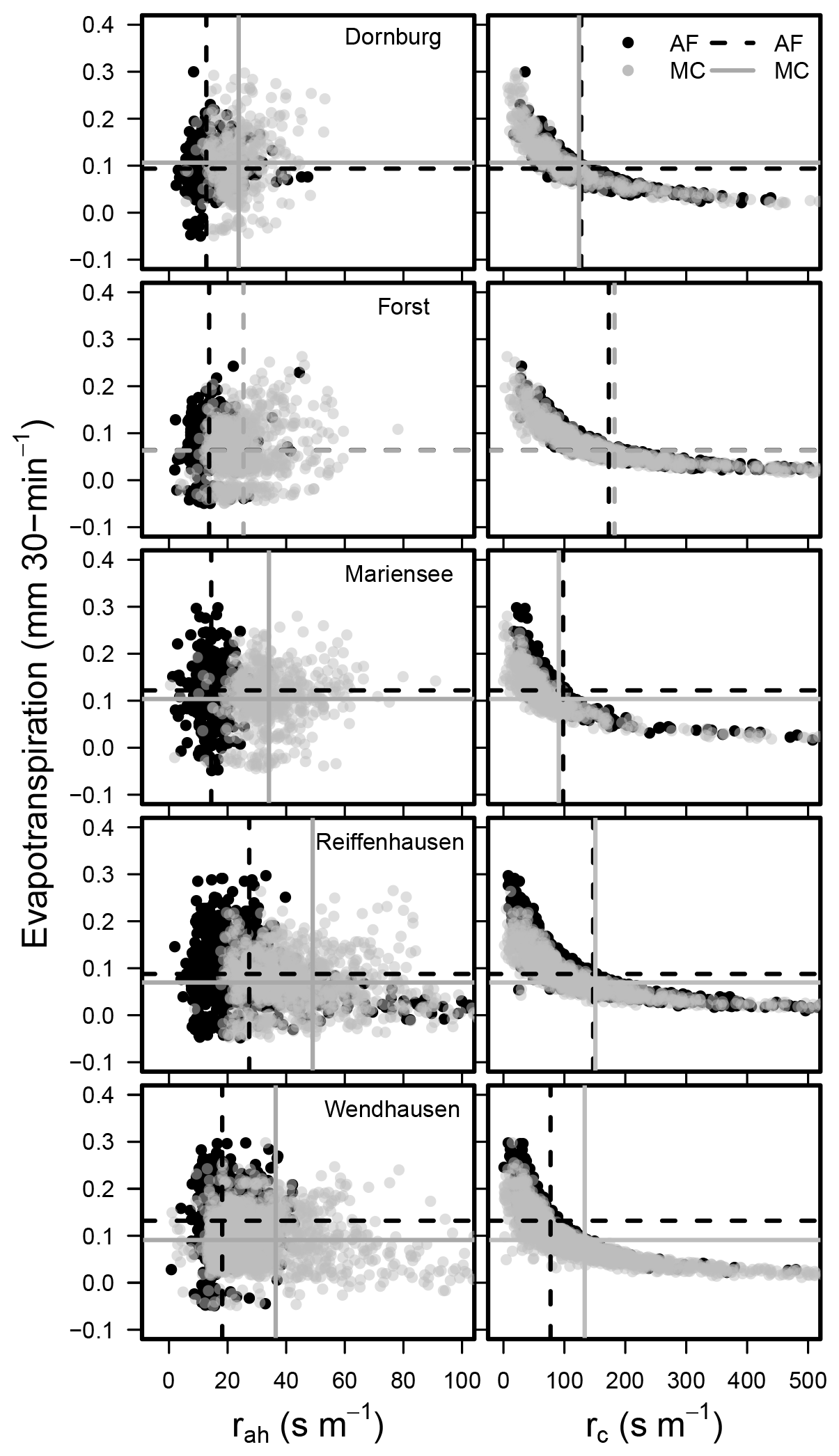
Figure 12 Half-hourly ET_EC-LC vs. aerodynamic resistance (r_ah; left) and canopy resistance (r_c; right) for all sites. The dashed grey line corresponds to the mean aerodynamic and canopy resistance and evapotranspiration at the AF system, and the dashed black line corresponds to the mean aerodynamic and canopy resistance and evapotranspiration at the MC system at the specific site. Only data corresponding to ideal ambient conditions are shown, e.g. global radiation (R_G≥400 W m⁻²), wind speed (u≥1 m s⁻¹), and vapour pressure deficit ($D=\mathrm{1}\pm \mathrm{0.3}$ kPa; Schmidt-Walter et al., 2014).

3.6 Uncertainty and limitations of ET measurements over AF

As outlined in the previous section, differences in annual sums of ET between the different land uses were small. Besides the discussed ecological reasons, we are aware of measurement errors due to the heterogeneous terrain (Foken, 2008b). The most critical assumptions of the eddy covariance method are horizontally homogeneous terrain and steady state ambient conditions (Foken et al., 2006; Foken, 2008b). It is assumed that the heterogeneities generate turbulent motions of a longer timescale than the commonly applied averaging period of half an hour. This is also strongly connected to horizontal advection, which is commonly not properly represented in eddy covariance flux measurements. Foken et al. (2006) noted that the eddy covariance method is the most accurate method, with errors between 5 % and 10 %, depending on the turbulent conditions. The errors are higher during the nighttime due to limited turbulent conditions, causing a common flux underestimation (Aubinet et al., 2010). But during the night especially ET is small, and the effect of high errors is small compared to the daytime conditions when ET is high.

For the low-cost eddy covariance set-up we anticipate higher errors compared to direct EC due to the limited time response of the thermohygrometer and, subsequently, higher spectral correction factors (Markwitz and Siebicke, 2019). We found that the effect of heterogeneity on ET is less important for EC-LC than the effect of different measurement heights (Markwitz and Siebicke, 2019). For a measurement height of 3.5 m, we found a latent heat flux underestimation compared to direct EC, and for a measurement height of 10 m, we found a slight latent heat flux overestimation (Table 4). At a lower height the contribution of small and high-frequency fluctuations to the energy spectrum is higher. Due to the limited time response of the thermohygrometer between 1.9 and 3.5 s (Markwitz and Siebicke, 2019), the high-frequency eddies cannot be adequately detected, and the signal losses are higher.

In contrast, ET_ECEB might be affected by greater errors than ET_EC-LC due to multiple error sources inferred from each of the energy balance components, the assumption of a fully closed energy balance, and resulting inaccuracies from the energy balance residual partitioning. For the ECEB set-up the heterogeneity of the landscape has a larger impact than for the EC-LC set-up, such as net radiation and ground heat flux measurements are not representative for the whole landscape.

Although errors for ET measurements with the respective set-ups can be large on a half-hourly timescale, for annual sums of ET the errors often compensate each other and are small relative to the measured signal (Hollinger and Richardson, 2005). As an example, we calculated the random error uncertainty after Hollinger and Richardson (2005) for the latent heat fluxes (LE_ECEB) from Dornburg AF for 2016. The larger the integration time (hourly, daily, and monthly), the smaller the random error. The magnitude of the random error was about 2.3 % (median over n=9) of the flux magnitude for monthly averages, 11.55 % (n=254) for daily averages, and 34.5 % (n = 12 191) for hourly averages. Hence, the random error for annual sums would be even smaller.

4 Conclusions

The main objective of the current work was to investigate the effect of AF on evapotranspiration in comparison to monoculture agriculture without trees. We performed evapotranspiration measurements at multiple sites, for 2 consecutive years, with a low-cost eddy covariance set-up and an eddy covariance energy balance set-up.

In the first part of this paper, we investigated the performance of the measurement set-ups. In comparison with direct eddy covariance measurements, the low-cost eddy covariance set-up captured the temporal variability in half-hourly ET rates with high coefficients of determination during a comparison measuring campaign. The ECEB set-up also represented the diel cycle of ET but was characterised by more scatter. We therefore conclude that the EC-LC set-up is a viable alternative compared to conventional eddy covariance set-ups, as this set-up represents the ET of the underlying ecosystem more accurately than the ECEB set-up.

In the second part of the paper, we focused on the question of whether AF systems have higher water losses to the atmosphere via ET compared to monoculture systems. Our results showed that differences in ET between AF and MC were small. Instead, we found higher evapotranspiration indices during a drier than normal year compared to a wet year across sites and methods. This shows that the potentially small effect from the trees on ET was overlaid by the effect of local climatic conditions. In addition, we found a similar plant physiological response to the AF and the MC systems which is characterised by small differences between canopy resistances.

Overall, we conclude that the inclusion of tree strips into the agricultural landscape has not resulted in higher water losses to the atmosphere via ET, and agroforestry can be a land use alternative to monoculture agriculture without trees.

Appendix A: Derivations

A1 Half-hourly ET rates and soil storage flux

Half-hourly evapotranspiration rates in units of mm 30 min⁻¹ were calculated from LE as follows:

$$\begin{array}{}\text{(A1)}& \begin{array}{rl}\mathrm{ET}& ={\displaystyle \frac{{\mathrm{LE}}_{\mathrm{ECEB}}\left(\mathrm{J}{\mathrm{kg}}^{-\mathrm{1}}{\mathrm{s}}^{-\mathrm{1}}\right)}{L\left(\mathrm{J}{\mathrm{kg}}^{-\mathrm{1}}\right)}}\cdot \mathrm{1800}\left(\mathrm{s}\mathrm{30}{\min }^{-\mathrm{1}}\right)\\ & \cdot {\displaystyle \frac{\mathrm{1}}{{\mathit{\rho }}_{{\mathrm{H}}_{\mathrm{2}}\mathrm{O}}}}\left({\mathrm{m}}^{\mathrm{3}}{\mathrm{kg}}^{-\mathrm{1}}\right)\cdot \mathrm{1000}\mathrm{mm}{\mathrm{m}}^{-\mathrm{1}},\end{array}\end{array}$$

with L (J kg⁻¹), the latent heat of vaporisation (Dake, 1972), depending on air temperature T (^∘C), as follows:

$$\begin{array}{}\text{(A2)}& {\displaystyle }L{\displaystyle }=(\mathrm{2.501}-\mathrm{0.00237}T)\times {\mathrm{10}}^{\mathrm{6}},\end{array}$$

and ${\mathit{\rho }}_{{\mathrm{H}}_{\mathrm{2}}\mathrm{O}}=\mathrm{1000}$ kg m⁻³ the density of liquid water.

The soil heat storage term has a major contribution to the unclosed energy balance (Foken, 2008a), and the magnitude of the soil heat storage is comparably larger than the other storage terms, i.e. the photosynthesis flux, the crop enthalpy change, the air enthalpy change, the canopy dew water enthalpy change, and the atmospheric moisture change (Jacobs et al., 2008). We used the ground heat flux (G) from the ground heat flux measurements, G_HFP (W m⁻²), at the sites and calculated the soil heat storage between the soil heat flux plate and the soil layer above, following Liebethal and Foken (2007) as follows:

$$\begin{array}{}\text{(A3)}& G=G_{\mathrm{HFP}}+\underset{z=-\mathrm{0.05}\mathrm{m}}{\overset{\mathrm{0}\mathrm{m}}{\int }}{c}_{\mathrm{v}}{\displaystyle \frac{\partial T}{\partial t}}\mathrm{d}z.\end{array}$$

The soil heat storage (second term on the right-hand side of Eq. A3) consists of the vertical integral of the change in temperature over time at depth z=0.02 m. c_v is the volumetric heat capacity of the soil, calculated from the soil components, i.e. organic, mineral, and water and their respective heat capacities. Soil texture and bulk densities are summarised in Table B2 and were provided by Göbel et al. (2018) and Marcus Schmidt (personal communication, Georg August University of Göttingen, Buesgen Institute, Soil Science of Tropical and Subtropical Ecosystems, 2018). Gaps in soil storage data were filled according to a multiple linear regression with soil storage vs. net radiation and ground heat flux. The multiple linear regression fitting parameters were derived from records when the soil storage, the net radiation, and the ground heat flux were available at the same time.

A2 Water vapour mole fraction $C_{{{\mathrm{H}}_{\mathrm{2}}\mathrm{O}}_{\mathrm{v}}}$ from the thermohygrometer

The derivation of the water vapour mole fraction ($C_{{{\mathrm{H}}_{\mathrm{2}}\mathrm{O}}_{\mathrm{v}}}$) from relative humidity, air temperature, and air pressure from the low-cost thermohygrometer was also presented in Markwitz and Siebicke (2019) and is given in this section.

The water vapour mole fraction was derived from the definition of the specific humidity (q) as being the quantity of water vapour per quantity of moist air. The latter two quantities were expressed as the density of water vapour (${\mathit{\rho }}_{{{\mathrm{H}}_{\mathrm{2}}\mathrm{O}}_{\mathrm{v}}}$) and moist air (ρ_m), respectively. The density of moist air is defined as the sum of the density of dry air (ρ_d) and the density of water vapour.

$$\begin{array}{}\text{(A4)}& \begin{array}{rl}q& ={\displaystyle \frac{{\mathit{\rho }}_{{{\mathrm{H}}_{\mathrm{2}}\mathrm{O}}_{\mathrm{v}}}}{{\mathit{\rho }}_{\mathrm{m}}}}\\ & ={\displaystyle \frac{{\mathit{\rho }}_{{{\mathrm{H}}_{\mathrm{2}}\mathrm{O}}_{\mathrm{v}}}}{{\mathit{\rho }}_{\mathrm{d}}+{\mathit{\rho }}_{{{\mathrm{H}}_{\mathrm{2}}\mathrm{O}}_{\mathrm{v}}}}}.\end{array}\end{array}$$

We then replaced the density of water vapour and the density of dry air in Eq. (A4) as per Eqs. (A5) and (A6), respectively, as follows:

$$\begin{array}{}\text{(A5)}& {\displaystyle }& {\displaystyle }{\mathit{\rho }}_{{{\mathrm{H}}_{\mathrm{2}}\mathrm{O}}_{\mathrm{v}}}={\displaystyle \frac{C_{{{\mathrm{H}}_{\mathrm{2}}\mathrm{O}}_{\mathrm{v}}}\cdot M_{{{\mathrm{H}}_{\mathrm{2}}\mathrm{O}}_{\mathrm{v}}}}{V_{\mathrm{m}}}}\text{(A6)}& {\displaystyle }& {\displaystyle }{\mathit{\rho }}_{\mathrm{d}}={\displaystyle \frac{p-e_{\mathrm{a}}}{R_{\mathrm{d}}\cdot T}},\end{array}$$

with the molar mass of water vapour, $M_{{{\mathrm{H}}_{\mathrm{2}}\mathrm{O}}_{\mathrm{v}}}=\mathrm{18.02}$ g mol⁻¹, and the molar volume of air, as follows:

$$\begin{array}{}\text{(A7)}& V_{\mathrm{m}}={\displaystyle \frac{\mathfrak{R}\cdot T}{p}}\left({\mathrm{m}}^{\mathrm{3}}{\mathrm{mol}}^{-\mathrm{1}}\right),\end{array}$$

the universal gas constant (ℜ=8.314 $\mathrm{J}{\mathrm{mol}}^{-\mathrm{1}}{\mathrm{K}}^{-\mathrm{1}}$) and the specific gas constant of dry air (R_d=287.058 $\mathrm{J}{\mathrm{kg}}^{-\mathrm{1}}{\mathrm{K}}^{-\mathrm{1}}$).

Solving Eq. (A4) for $C_{{{\mathrm{H}}_{\mathrm{2}}\mathrm{O}}_{\mathrm{v}}}$ leads to the water vapour mole fraction as follows:

$$\begin{array}{}\text{(A8)}& C_{{{\mathrm{H}}_{\mathrm{2}}\mathrm{O}}_{\mathrm{v}}}={\displaystyle \frac{q\mathfrak{R}(p-e_{\mathrm{a}})}{p{M}_{{{\mathrm{H}}_{\mathrm{2}}\mathrm{O}}_{\mathrm{v}}}{R}_{\mathrm{d}}(\mathrm{1}-q)}}.\end{array}$$

The specific humidity in Eq. (A8) was calculated as a function of relative humidity, temperature, and air pressure measurements from the thermohygrometer as follows:

$$\begin{array}{}\text{(A9)}& q=\mathrm{0.622}\cdot {\displaystyle \frac{e_{\mathrm{a}}}{p}}.\end{array}$$

The actual vapour pressure (e_a; kPa) in Eq. (A9) was calculated from an approximation of the saturation vapour pressure (e_*(T); Stull, 1989) and from relative humidity (RH) as follows:

$$\begin{array}{}\text{(A10)}& {\displaystyle }e& {\displaystyle }={\displaystyle \frac{\mathrm{RH}\cdot e_{*}\left(T\right)}{\mathrm{100}}}\text{(A11)}& {\displaystyle }{e}_{*}\left(T\right)& {\displaystyle }=\mathrm{0.6112}\exp \left({\displaystyle \frac{\mathrm{17.67}T}{(T+\mathrm{273.15})-\mathrm{29.66}}}\right).\end{array}$$

A3 Canopy resistance

The Penman–Monteith equation for the latent heat flux of a canopy (Monteith, 1965) is as follows:

$$\begin{array}{}\text{(A12)}& {\displaystyle }\mathrm{LE}{\displaystyle }={\displaystyle \frac{s(R_{\mathrm{N}}-G)+c_{\mathrm{p}}D{g}_{\mathrm{ah}}}{s+\mathit{\gamma }(\mathrm{1}+g_{\mathrm{ah}}/g_{\mathrm{c}})}},\end{array}$$

with the vapour pressure deficit ($D=e_{*}\left(T\right)-e_{\mathrm{a}}$; hPa), the heat capacity at constant pressure (c_p=1005 J (kg K)⁻¹), and the psychrometer constant ($\mathit{\gamma }=\left(c_{\mathrm{p}}{P}_{\mathrm{A}}\right)/\left(L\mathrm{0.622}\right)$).

The slope of the saturation vapour pressure curve (s) is as follows:

$$\begin{array}{}\text{(A13)}& s={\displaystyle \frac{\mathit{\epsilon }L{q}_{\mathrm{sat}}}{R_{\mathrm{v}}T}},\end{array}$$

with ε=0.622 and the specific humidity at saturation ($q_{\mathrm{sat}}=\mathit{\epsilon }{e}_{*}\left(T\right)/P_{\mathrm{A}}$) as a function of temperature.

Rearranging Eq. (A12) yields the canopy resistance (r_c; s m⁻¹) as follows:

$$\begin{array}{}\text{(A14)}& r_{\mathrm{c}}={\displaystyle \frac{\mathrm{1}}{g_{\mathrm{c}}}}={\displaystyle \frac{s/\mathit{\gamma }+\mathrm{1}}{g_{\mathrm{ah}}}}[{\displaystyle \frac{s/\mathit{\gamma }(R_{\mathrm{N}}-G)}{(s/\mathit{\gamma }+\mathrm{1})\mathrm{LE}}}-\mathrm{1}]+{\displaystyle \frac{c_{\mathrm{p}}D}{\mathit{\gamma }\mathrm{LE}}}.\end{array}$$

The aerodynamic conductance for heat is as follows:

$$\begin{array}{}\text{(A15)}& \begin{array}{rl}{g}_{\mathrm{ah}}& ={\displaystyle \frac{\mathrm{1}}{r_{\mathrm{ah}}}}\\ & ={\displaystyle \frac{{\mathit{\kappa }}^{\mathrm{2}}u}{\left(\ln \right(\frac{z-d}{z_{\mathrm{0}\mathrm{m}}})-{\mathit{\psi }}_{\mathrm{m}}(\mathit{\zeta }\left)\right)\left(\ln \right(\frac{z-d}{z_{\mathrm{0}\mathrm{h}}})-{\mathit{\psi }}_{\mathrm{h}}(\mathit{\zeta }\left)\right)}},\end{array}\end{array}$$

with the von Kármán constant (κ=0.4), the horizontal wind velocity (u; m s⁻¹), the measurement height (z; m) and the displacement height (d; m), estimated as 70 % of the canopy height, and the roughness length for momentum transport (z_0m), estimated as 10 % of the canopy height and the roughness length for heat transport (z_0h), estimated as 10 % of z_0m. ψ_m(ζ) is the universal function for momentum, and ψ_h(ζ) is the universal function for heat. ψ_m(ζ) and ψ_h(ζ) depend on atmospheric stability with the stability parameter $\mathit{\zeta }=(z-d)/L$, including the Monin–Obukhov length (L). ψ_m and ψ_h were calculated as follows:

$$\begin{array}{}\text{(A16)}& {\displaystyle }{\mathit{\psi }}_{\mathrm{m}}\left(\mathit{\zeta }\right)=\left\{\begin{array}{ll}\mathrm{2}\ln \left[\right(\mathrm{1}+x)/\mathrm{2}]+\ln \left[\right(\mathrm{1}+x^{\mathrm{2}})/\mathrm{2}]& \text{for }\mathit{\zeta }<\mathrm{0}\\ -\mathrm{2}\arctan \left(x\right)+\mathit{\pi }/\mathrm{2}& \\ \\ -\mathrm{5}\mathit{\zeta }& \text{for }\mathit{\zeta }\ge \mathrm{0}\end{array}\right.\text{(A17)}& {\displaystyle }{\mathit{\psi }}_{\mathrm{h}}\left(\mathit{\zeta }\right)=\left\{\begin{array}{ll}\mathrm{2}\ln \left[\right(\mathrm{1}+x^{\mathrm{2}})/\mathrm{2}]& \text{for }\mathit{\zeta }<\mathrm{0}\\ -\mathrm{5}\mathit{\zeta }& \text{for }\mathit{\zeta }\ge \mathrm{0},\end{array}\right.\end{array}$$

with x = $(\mathrm{1}-\mathrm{16}\mathit{\zeta }{)}^{\mathrm{1}/\mathrm{4}}$ (Bonan, 2016; Businger et al., 1971; Stull, 1989).

Appendix B: Tables

Table B1 Temporal extent of the EC measurement campaigns.

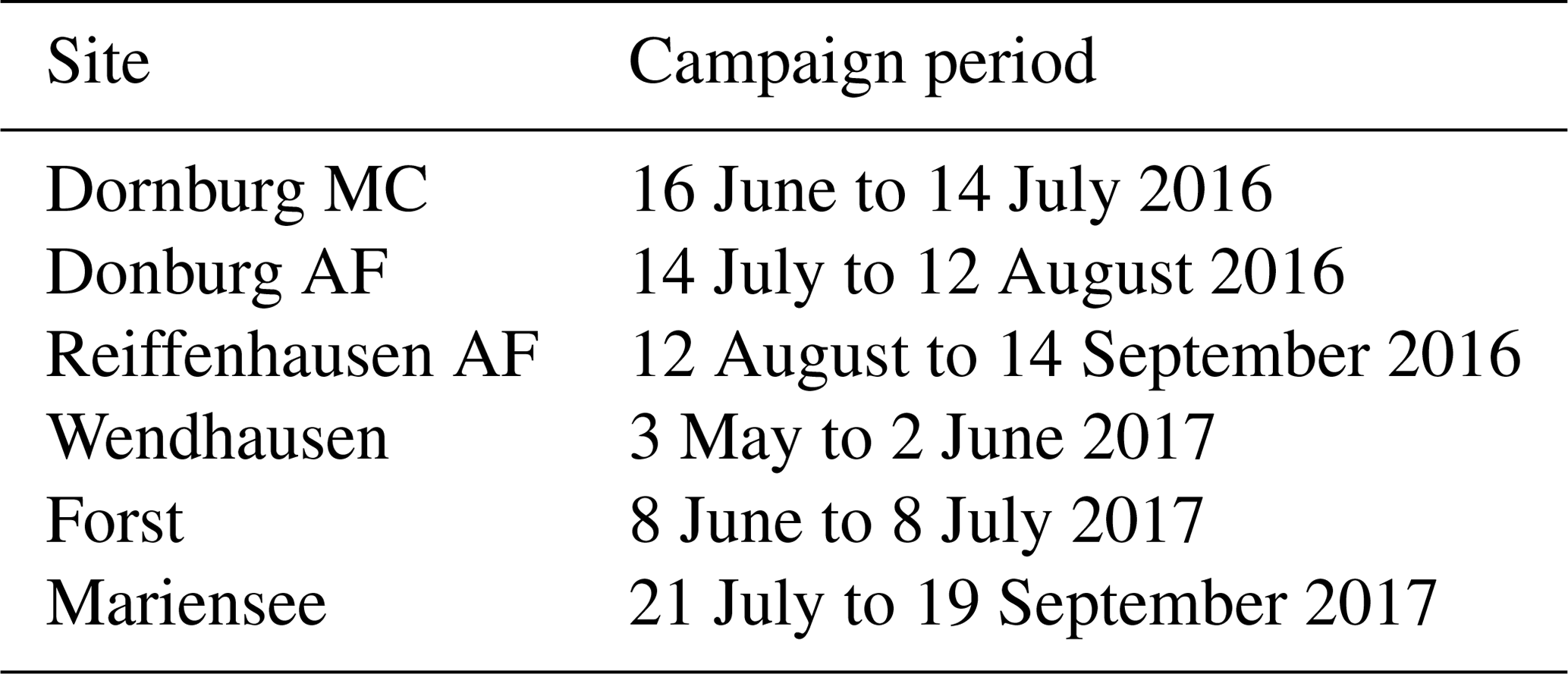
Table B2 Site-specific soil characteristics, with the soil texture being representative for the top soil column of 0.3 m. The bulk density is representative for the top soil column of 0.05 m. Data provided by Göbel et al. (2018) and Marcus Schmidt (personal communication, Georg August University of Göttingen, Buesgen Institute, Soil Science of Tropical and Subtropical Ecosystems, 2018).

Appendix C: Figures

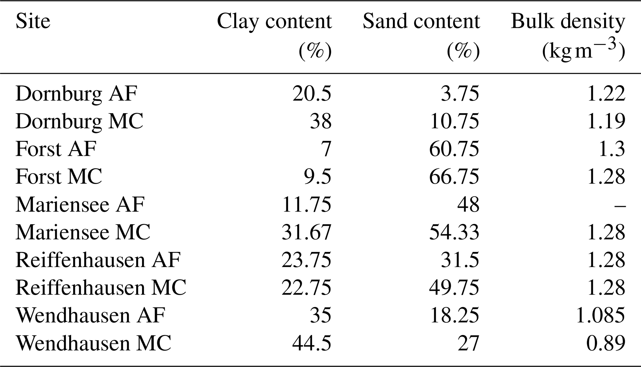
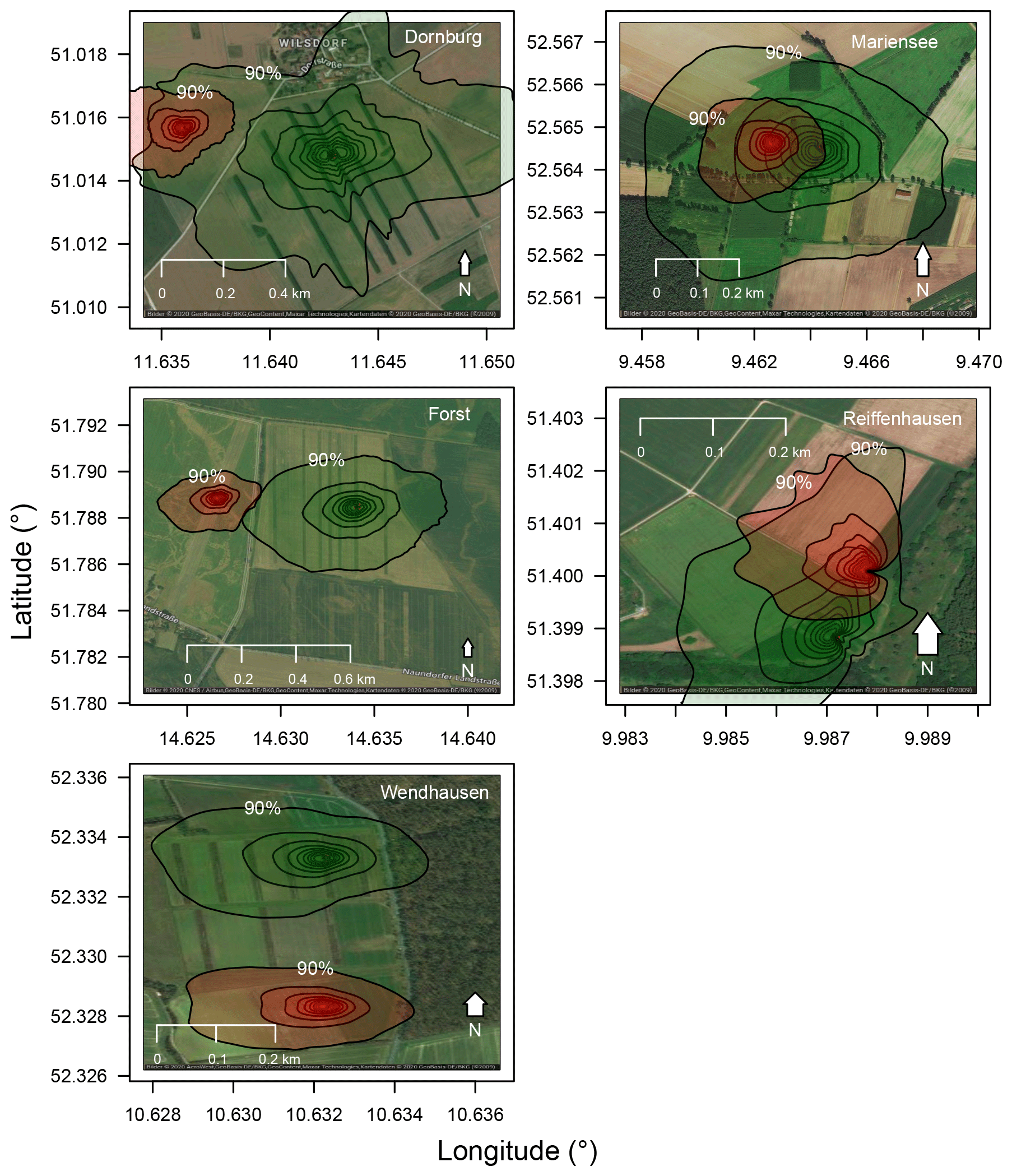
Figure C1 Flux footprint climatology for all sites and all available data during the years 2016 and 2017. Green shaded footprints correspond to the agroforestry system, and red shaded footprints correspond to the monoculture system. For the analysis only daytime data were used (R_G>20 W m⁻²). Aerial photographs originate from Google Maps and Google Earth. © Google 2020.

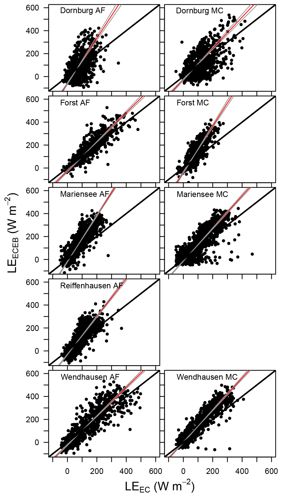
Figure C2 Scatter plot of LE_ECEB vs. LE_EC for all sites. The red line denotes the best fit line, with grey lines as the ±2.5 % confidence interval lines, and the solid black lines corresponding to the 1 : 1 line. Data from Reiffenhausen MC are missing due to the unavailability of a campaign.

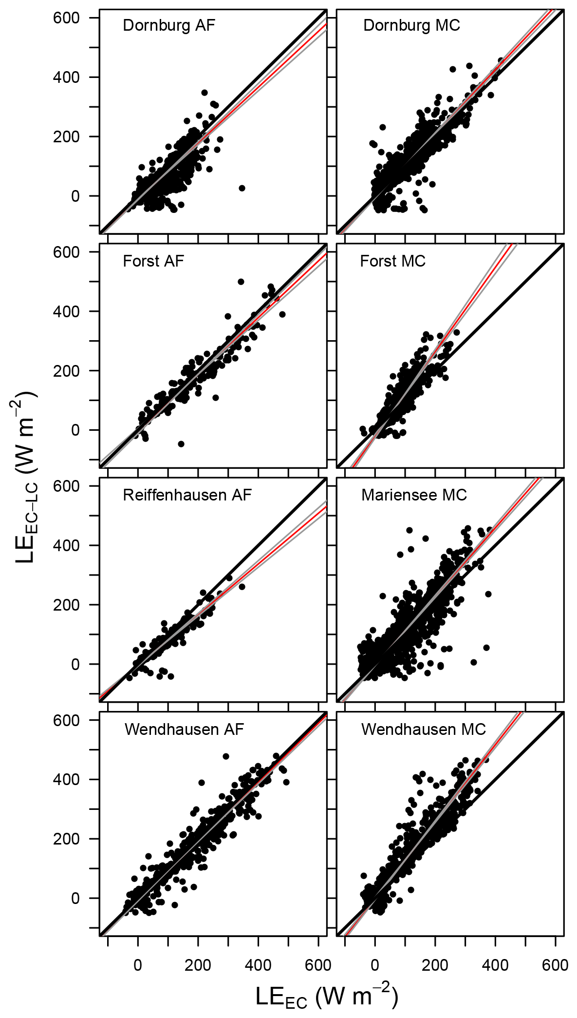
Figure C3 Scatter plot of LE_EC-LC vs. LE_EC for all sites. The red line denotes the best fit line, with grey lines as the ±2.5 % confidence interval lines, and the solid black lines corresponding to the 1 : 1 line. Data from Reiffenhausen MC are missing due to the unavailability of a campaign, and LE_EC-LC from Mariensee AF is missing due to sensor malfunctions.

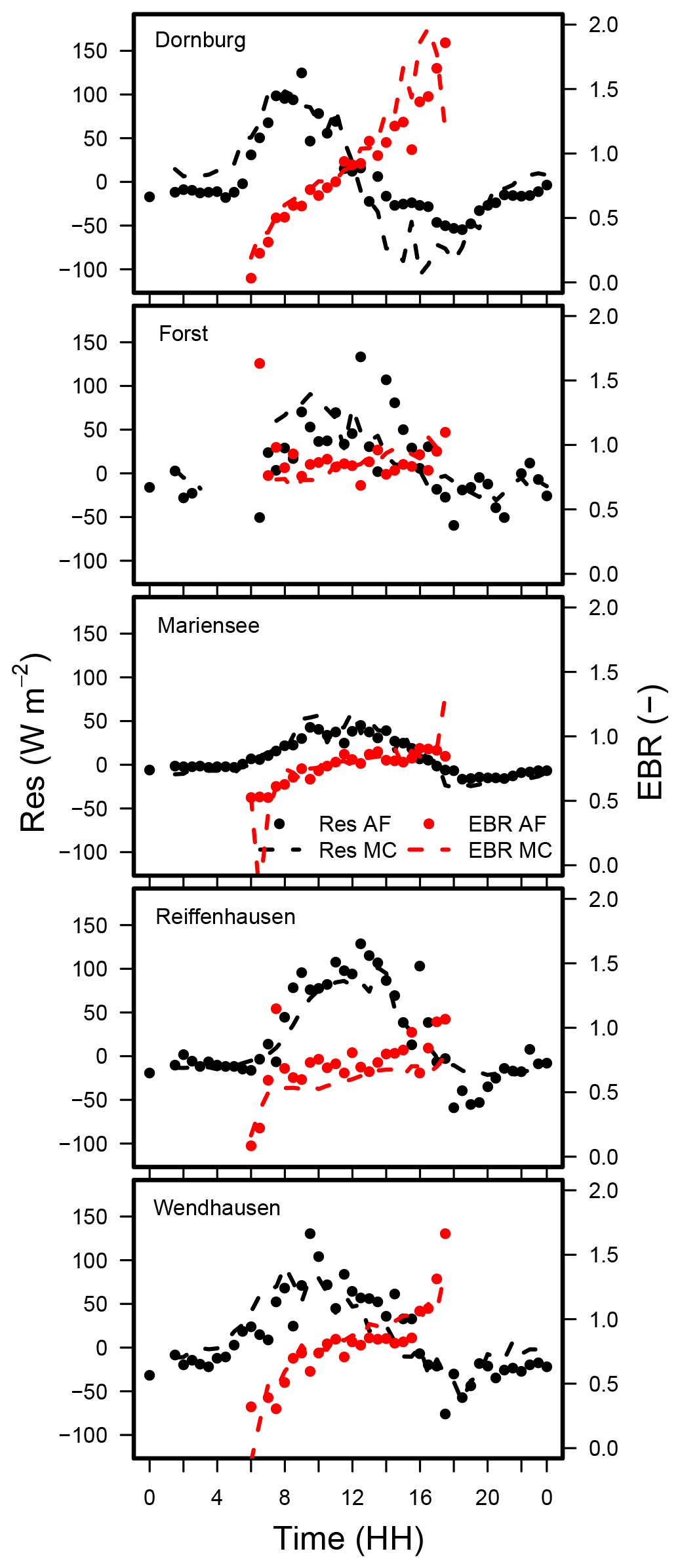
Figure C4 Median diel cycle of the energy balance ratio (EBR), and the diurnal cycle of the residual energy for the AF and the MC systems at all sites. LE was obtained by EC-LC. Data from Mariensee AF are from 23 March to 20 November 2016, and at Reiffenhausen MC the analyses are based on data collected from 7 April to 31 December 2016 because no data were available during the campaigns.

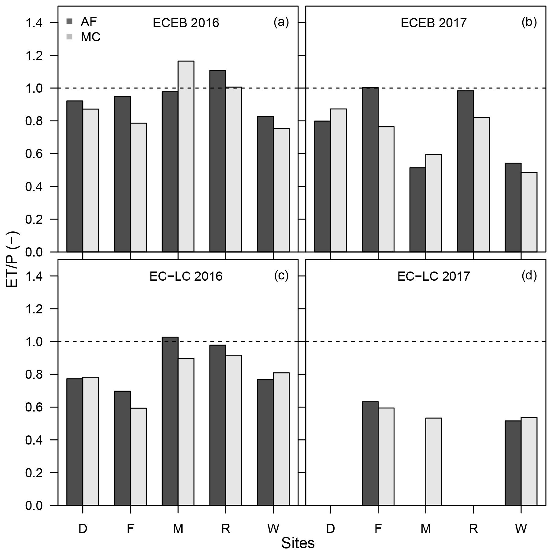
Figure C5 Bar plot of the evapotranspiration index for the ECEB method for the years 2016 (a) and 2017 (b) and for the EC-LC method for 2016 (c) and 2017 (d) for the sites, e.g. Dornburg (D), Forst (F), Mariensee (M), Reiffenhausen (R), and Wendhausen (W). The dashed line indicates an evapotranspiration index of one. Evapotranspiration indices for Dornburg AF and MC, Mariensee AF, and Reiffenhausen AF and MC in 2017 are missing due to instrument malfunctions.