Technical note: Seamless gas measurements across the land–ocean aquatic continuum – corrections and evaluation of sensor data for CO₂, CH₄ and O₂ from field deployments in contrasting environments

The ocean and inland waters are two separate regimes, with concentrations in greenhouse gases differing on orders of magnitude between them. Together, they create the land–ocean aquatic continuum (LOAC), which comprises itself largely of areas with little to no data with regards to understanding the global carbon system. Reasons for this include remote and inaccessible sample locations, often tedious methods that require collection of water samples and subsequent analysis in the lab, and the complex interplay of biological, physical and chemical processes. This has led to large inconsistencies, increasing errors and has inevitably lead to potentially false upscaling. A set-up of multiple pre-existing oceanographic sensors allowing for highly detailed and accurate measurements was successfully deployed in oceanic to remote inland regions over extreme concentration ranges. The set-up consists of four sensors simultaneously measuring pCO₂, pCH₄ (both flow-through, membrane-based non-dispersive infrared (NDIR) or tunable diode laser absorption spectroscopy (TDLAS) sensors), O₂ and a thermosalinograph at high resolution from the same water source. The flexibility of the system allowed for deployment from freshwater to open ocean conditions on varying vessel sizes, where we managed to capture day–night cycles, repeat transects and also delineate small-scale variability. Our work demonstrates the need for increased spatiotemporal monitoring and shows a way of homogenizing methods and data streams in the ocean and limnic realms.

1 Introduction

Both carbon dioxide (CO₂) and methane (CH₄) are significant players in the Earth's climate system, with 2016 being the first full year in which atmospheric CO₂ rose above 400 parts per million (ppm), with an average of 402.8 ± 0.1 ppm (Le Quéré et al., 2018). Since 1750, it has risen from 277 ppm. A similar trend has been seen with CH₄, which has increased by 150 % in the atmosphere to 1803 parts per billion (ppb) between 1750 and 2011 (Ciais et al., 2013), with an acceleration in recent years to 1850 ppb in 2017 (Nisbet et al., 2019). With the oceans being a sink for an estimated ∼ 24 % of anthropogenic CO₂ emissions (Friedlingstein et al., 2019), they have been under continuous observation and study, resulting in the collection of large global databases (e.g., Takahashi et al., 2009; Bakker et al., 2016). Such observations have shown both regional and/or temporal variabilities between a source and sink for CO₂, yet it is typically a low to moderate CH₄ source (∼ 0.4–1.8 Tg CH₄ yr⁻¹; Bates et al., 1996; Borges et al., 2018; Rhee 2009), increasing in coastal regions (Bange, 2006). Inland waters, however, are a different story, and although it has been known for over 50 years that they are mostly supersaturated with CO₂ (Park, 1969), up until recently their budgets have been of relatively little focus. Although regions such as lakes, rivers and reservoirs have been recognized as significant players in the carbon budget over the past couple of decades (see Carpenter et al., 1995; Cole and Caraco, 1998; Caraco, 2001 with updates and reviews from Tranvik et al., 2009; Raymond et al., 2013 and Regnier et al., 2013), compared to the ocean data sets, having quantified and consistent data and consensus within these regions is still in the relatively early stages. Global CO₂ and CH₄ emissions from inland waters are estimated at 2.1 Pg C yr⁻¹ (Raymond et al., 2013) and 0.7 Pg C yr⁻¹ (Bastviken et al., 2011), respectively. Mixing regimes (e.g. deltas and estuaries) and streams and smaller bodies of water are known to be overly important within these inland systems (Holgerson and Raymond, 2016; Natchimuthu et al., 2017; Grinham et al., 2018), yet there is very little data coverage with respect to both of these parameters (Borges et al., 2018) – even more so when they are evaluated together. Therefore, a specific need exists for high-resolution spatiotemporal measurements in regimes of highly dynamic, varying pCO₂ concentrations (Yoon et al., 2016; Paulsen et al., 2018; Friedlingstein et al., 2019).

One issue leading to little data coverage is that the combination of both inland waters and the ocean, i.e. the land–ocean aquatic continuum (LOAC), is usually not studied continuously but rather split between oceanographers and limnologists. Although significant progress has been made in recognizing the importance of the LOAC as a whole system (e.g. Raymond et al., 2013; Regnier et al., 2013; Downing 2014; Palmer et al., 2015; Xenopoulos et al., 2017), huge knowledge gaps are still present, particularly related to limited field data availability (Meinson et al., 2016). Often, this is due to different measuring techniques and protocols, both with respect to in situ/autonomous observations and the collection of discrete data. This has been previously noted, through blind or spot sampling having large effects on the overall measured results, potentially leading to under-/overestimations in concentrations and fluxes (Richey et al., 2002; Abril et al., 2014; Canning et al., 2020b). Furthermore, this is further complicated by pCO₂, pCH₄ and dissolved O₂ being controlled by several factors, including biological effects, vertical and lateral mixing and temperature-dependent thermodynamic effects (Bai et al., 2015). These effects are exacerbated within inland waters where variability is far higher due to variations in environmental conditions and the magnitude of biological processes and anthropogenic influences (Cole et al., 2007). The high spatial and temporal variability within the inland/mixing waters (Wehrli, 2013) only increases these difficulties, ultimately leading to the interface between the ocean and inland to be considered one of the hardest systems to observe accurately and adequately. This has led to limitations and lack of verifications, leading to errors, discrepancies and uncertainties involved in scaling up the data. Inland waters tend to exhibit extreme ranges of CO₂ partial pressure (pCO₂, <100 to >10 000 µatm; this study; Abril et al., 2015; Ribas-Ribas et al., 2011) in comparison to oceanic waters (∼ 100–700 µatm; Valsala and Maksyutov, 2010), while also showing extreme variabilities for both O₂ and CH₄. Given the much smaller concentration changes and gradients, oceanic sensors and methods have been specifically tailored to assure high accuracy over oceanic concentration ranges, in comparison to inland waters.

One way of tackling these limitations and measurement technique differences is through sensors, ensuring a unified way of measuring with well-constrained accuracy and precision. In specific regions, this has become more widespread and reviewed numerous times within the coastal and open ocean (see Atamanchuk et al., 2015; Clarke et al., 2017). Multiple seagoing methods have been applied since the 1960s (see examples in Takahashi, 1961; DeGrandpre et al., 1995; Waugh et al., 2006; Pierrot et al., 2009; Schuster and Körtzinger, 2009; Becker et al., 2012) to measure and estimate greenhouse gases, such as CO₂, across a variety of aquatic regions. Inland water investigations have also seen clear progress with the development of continuous, autonomous measurement techniques (e.g. DeGrandpre et al., 1995; Baehr and DeGrandpre, 2004; Crawford et al., 2014; Meinson et al., 2016; Brandt et al., 2017). Yet, only few studies have employed membrane-based equilibration sensors with non-dispersive infrared spectrometry (NDIR) detection (e.g. Johnson et al., 2009; Bodmer et al., 2016; Yoon et al., 2016; Hunt et al., 2017), with some adapting atmospheric sensors (see Bastviken et al., 2015). These methods often focus on only one gas (usually CO₂), and none of these methods mentioned cover both water regimes (ocean to inland), potentially leading to missed mixing regime regions. On top of this, spatiotemporal data coverage has been noted to be sparse (Yoon et al., 2016) and is needed to advance our budget accuracies and understanding.

Given the biological and physical parameters of inland waters, multi-gas analyses is the way forward, which was previously noted in the work of Brennwald et al. (2016), where they worked on the development of the membrane inlet mass spectrometry (MIMS) known as miniRuedi. This system measured as a nearly fully autonomous multi-gas mass spectrometer; however, despite advances in both inert and reactive gas measurements, the need for a filter and gas standards for extreme gradients gives this set-up a disadvantage in highly diverse inland waters. This highlights one issue with extremely variable environments and shows that there is need to develop a robust, fully autonomous sensor system that is portable enough for small and simple platforms. The development needs to be able to measure a full range of concentrations accurately and precisely, which is usually out of the specifications of sensors designed for one region. It needs to have the potential to measure multiple gases and ancillary parameters in unison across salinity and regional boundaries (including extreme concentrations), enabling us to measure throughout the LOAC. These efforts would hopefully bridge the ocean–limnic gap both technically and by reducing discrepancies and errors while having high-resolution, real-time measurements. To be accepted within both inland waters and the ocean, it needs to be within oceanic specifications while being able to handle larger concentration ranges. This is essential for improved monitoring, potentially avoiding spot sampling bias, providing in-need high-quality spatiotemporal variability data, tracking the global carbon budget (Le Quéré et al., 2018) and potentially applying it in areas of the highest uncertainties with potentially high anthropogenic input (Schimel et al., 2016).

Here we used state-of-the-art, membrane-based equilibrator non-dispersive infrared (NDIR) and tunable diode laser absorption spectroscopy (TDLAS) sensors for pCO₂ and pCH₄, respectively, which uses an oxygen optode and a thermosalinograph to create a set-up allowing measurements in a continuous flow-through system. To assess the versatility, performance, portability and measurement quality of the set-up, it was deployed across the three main aquatic environments, namely oceanic, brackish and limnic. We present the technical findings from the campaigns, showing the need for such high-resolution combined gas data on a larger spatiotemporal scale; however, biogeochemical implications will not be further investigated. The primary objective of the work presented here was, with the use of oceanic, state-of-the-art tested sensors, to realize a fully versatile, portable and robust flow-through system to accurately, autonomously and simultaneously measure multiple dissolved gases (CO₂, CH₄ and O₂) and ancillary parameters (temperature and salinity) across the full range of salinities. The second was to assess the potential for high-quality spatiotemporal data extraction. The set-up was subsequently deployed in each region of selected salinities (ocean, brackish and limnic waters) to allow for both spatial and temporal measurements. Extensive post-campaign corrections were assessed to see the need for their adaptation over all the regions, and for the more precise corrections, small-scale variability was used. Discrete samples were collected, and reference systems were deployed alongside to provide quality assessment of the performance of the flow-through set-up.

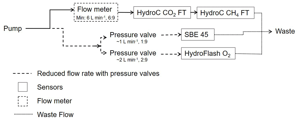
Figure 1 Flow schematic of the set-up, including minimal flow ratios. The flow rate was measured only for the main flow. For the side flows, the rate was adjusted, by pressure valves, to be a fraction (i.e. 1:9 and 2:9 for L min⁻¹) of the total flow.

2 Material and methods

2.1 Sensors and ranges

The set-up featured four separate sensors measuring three dissolved gases and standard hydrographic parameters (Table 1).

The CONTROS HydroC^® CO₂ FT (HC–CO₂) and CONTROS HydroC^® CH₄ FT (HC–CH₄) (formerly Kongsberg Maritime Contros GmbH, Kiel, Germany; now -4H- JENA Engineering GmbH, Jena, Germany, and hereinafter -4H- JENA) are both commercially manufactured sensors which use membrane-based equilibrators combined with NDIR and TDLAS gas detectors, respectively. Both sensors are of the flow-through type in which water is pumped through a plenum, with a planar semi-permeable membrane, across which dissolved gas partial pressure equilibrium is established with the headspace behind, as described by Fietzek et al. (2014). The sensors were factory calibrated before and after each cruise (Romanian campaigns all together), and the calibration polynomials were provided (in case of the pCO₂ sensor) by the manufacturer.

The CONTROS HydroFlash^® O₂ (formerly Kongsberg Maritime Contros GmbH, Kiel, Germany; hereinafter KMCON) was an optical sensor (optode) based on the principle of fluorescence quenching (see Bittig et al., 2018b, for an optode technology review). As the sensor was only available as a submersible type, a flow-through cell was built around the sensor head for integration into the flow-through system.

The SBE 45 micro thermosalinograph (Sea-Bird Scientific, Bellevue, WA, USA) was used to measure temperature and conductivity to calculate salinity. All sensor frequencies depended on cruise type and were set between one reading output per minute to one reading per second (oceanic to inland waters).

Table 1 Sensors and their manufacturer specifications, along with calibration range (for the CONTROS HydroC^® CO₂ FT and CH₄ FT, factory calibration ranges were specific to the campaigns).

^a -4H- JENA Engineering GmbH, Jena, Germany (formerly Kongsberg Maritime Contros GmbH, Kiel, Germany). ^b Formerly Kongsberg Maritime Contros GmbH, Kiel, Germany.
^c Flow through. ^d Sea-Bird Scientific, Bellevue, WA, USA.

2.2 Initial procedures and background

Initial experiments were conducted within the laboratory at GEOMAR, Kiel, Germany, and during short sea trials on board research vessel (RV) Littorina in 2016 to ensure the optimal performance of all sensors (data not shown here). HC–CO₂ was placed within the set-up upstream of HC–CH₄ due to higher sensitivity and the dependence of the parameter pCO₂ on temperature changes. The water flow was split between sensors, due to differing flow range requirements. A flow meter and pressure valves were installed to provide optimal flow speeds, as shown in the schematic of the overall set-up (Fig. 1).

Depending on the vessel type and the location of the measurement system contained therein, the pump was placed either in the moon pool of the ship or at the front of the boat (limnic cruises; see Table 2). The total flow was regulated by multiple pressure valves to a pump rate of approximately 9–10 L min⁻¹. The HC–CO₂ and HC–CH₄ show a distinct dependence on their response time (RT) and on the water flow rate, with the demand for the HC–CO₂ flow rates ranging from 2–16 L min⁻¹ (manufacturer recommendation is 5 L min⁻¹) and flow rates for the HC–CH₄ ranging from 6–16 L min⁻¹. Based on this information, combined with preliminary testing and power accessibility considerations across all regions, 6 L min⁻¹ was used as the target flow rate for the HC–CO₂ and HC–CH₄. Data acquired with any flow rate below 5 L min⁻¹ were flagged as being questionable as they may have contributed to increased errors.

The data were logged on an internal logger for the HC–CO₂ and HC–CH₄ in unison and displayed live using the CONTROS DETECT software. The SBE thermosalinograph and HydroFlash O₂ were logged on SeatermV2 software and a terminal programme (Tera Term), respectively. The sensors have the ability to set the timestamps for logged data, allowing alignment among all sensor systems and/or local time for discrete sample collection. Water flow was measured using LabJack software, and any power cuts (or other circumstances such as boats passing near to the house boat during the limnic cruises) were logged manually to ensure the best-quality outcome from the data processing which is described in the next sections.

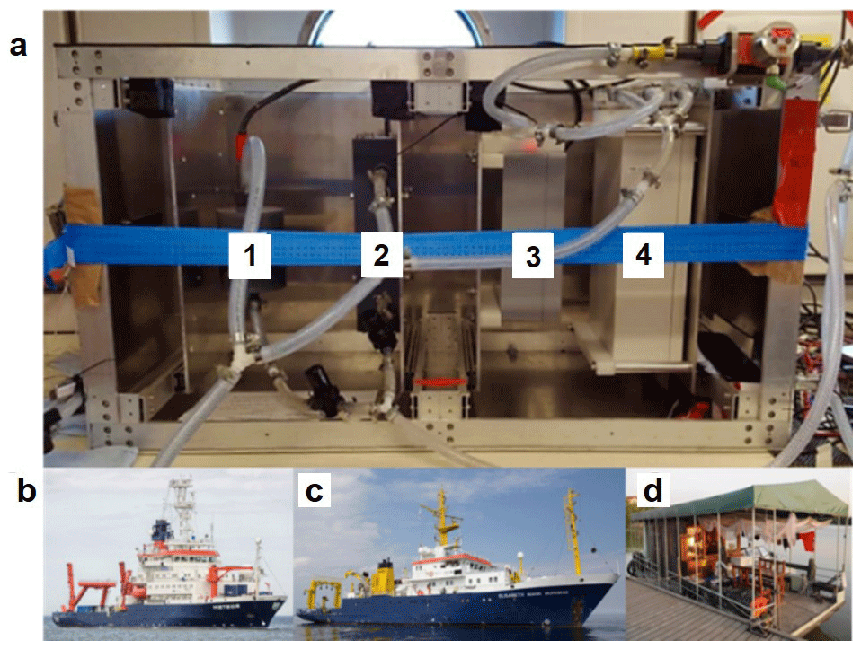
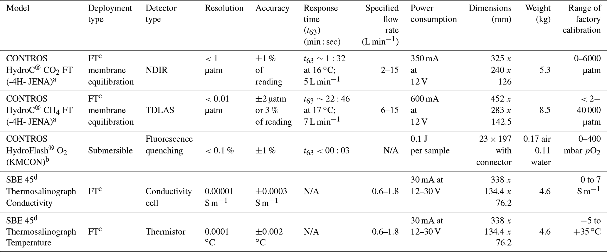
Figure 2 Complete flow-through set-up (a) in operation on board RV Meteor, indicating the easily accessible sensors for O₂ (1), T and S (2), and pCO₂ (3) and CH₄ (4). Besides the operation on RV Meteor, M133, (b) across the Atlantic, the set-up was also deployed on RV Elisabeth Mann Borgese, EMB 142, (c) within the Baltic Sea and on a houseboat in the Danube Delta (d), Romania, for spring (Rom1), summer (Rom2) and autumn (Rom3).

The set-up was tested in the following three different locations: the South Atlantic Ocean (oceanic), western Baltic Sea (brackish) and the Danube river delta, Romania, (limnic) between 2016 and 2017 (Figs. 2 and 3). Although, in brackish water regions like the Baltic Sea, the same measurement techniques for many instruments and sampling methods as those within the ocean are used, certain techniques (e.g. alkalinity titration) generally need special adaption for the low-salinity range. The different deployments ensured the sensors were tested in the field across the full salinity range, from freshwater to seawater, from moderate to tropical temperatures and from low concentrations near atmospheric equilibrium to extreme cases of supersaturation (CH₄ and CO₂) or undersaturation (CO₂ and O₂). The choice of cruises also allowed testing of the versatility of the set-up by deploying it on a range of vessel types (see Fig. 2, Table 2 and Sect. 2.3).

2.3 Campaigns

2.3.1 Meteor cruise M133 to the South Atlantic (oceanic)

The system was set up on the RV Meteor (cruise M133) during the South Atlantic Crossing (SACROSS) campaign, from Cape Town, South Africa, to Islas Malvinas, Argentina, between 15 December 2016 and 13 January 2017 (open to shelf oceanic waters). Discrete samples were collected throughout the cruise for total alkalinity (TA), dissolved inorganic carbon (DIC), CH₄ and O₂. The water was pumped up by means of a submersible pump installed in the ship's moon pool at about 5.7 m depth. The system logged once every minute, which was deemed sufficient until the Patagonian Shelf was reached, where the measurement frequency was increased to 1 Hz. Sea surface temperature data were measured with a temperature sensor (SBE 38; Sea-Bird Scientific, Bellevue, WA, USA) installed at the seawater intake in the moon pool, which was used for temperature correction of the flow-through system data. Sea surface salinity was taken from the ship's thermosalinograph (SBE 21; SeaCAT thermosalinograph (TSG); Sea-Bird Scientific, Bellevue, WA, USA) located within the mess room, and the water inlet was located on the bulbous bow. These salinity data were used for the carbonate system calculations related to the discrete reference. CH₄ data collected during this cruise were not used due to an internal issue of the detector related to absorption peak identification. These data were automatically flagged within the sensor diagnostic values and subsequently excluded. This issue was fixed for the limnic campaigns by the installation of a reference gas cell in the absorption path of the detector.

2.3.2 Elisabeth Mann Borgese cruise EMB 142 to the western Baltic Sea (brackish)

The sensor package was run on board the RV Elisabeth Mann Borgese (EMB 142) during a cruise to the western Baltic Sea between 15 and 22 October 2016 (brackish waters). The cruise was one of the main field activities of the Scientific Committee on Oceanic Research (SCOR) working group 142 (under the project titled “Dissolved N₂O and CH₄ measurements: Working towards a global network of ocean time series measurements of N₂O and CH₄”) and was entirely dedicated to the inter-comparison of continuous and discrete N₂O and CH₄ measurement techniques (see Wilson et al., 2018), but some of the systems also measured pCO₂ continuously. Discrete samples were collected for validation of the CO₂ and CH₄ sensors. All analysers and the discrete sampling line were connected to the same water supply from a submersible pump system installed in the ship's moon pool (depth 3 m), ensuring that the same water was used by all groups. A back-pressure regulation system assured the independent flow assurance of the individual set-ups. The sensors logged continuously at a rate of between once per second and once per minute, depending on local variability. During this cruise, only half the CH₄ data were used due the same technical reason as stated for the oceanic cruise.

Figure 3 Transects for all test sites. (a) Oceanic – South Atlantic; RV Meteor, cruise M133; ocean (Cape Town, South Africa, to Stanley, Islas Malvinas). (b) Brackish – RV Elisabeth Mann Borgese, cruise EMB 142; western Baltic Sea. (c) Limnic – Rom1–3; Danube Delta, Romania. Orange circles, labelled 1 through 4, show the stations of stationary overnight stops (see Fig. 11). For further information, see Table 2.

2.3.3 Romania 1–3 cruises in the Danube river delta, Romania (limnic)

Campaigns over three consecutive seasons were conducted during three field campaigns throughout the Danube Delta in Romania (limnic) in 2017, namely during spring (Rom1 – 17–26 June 2017), summer (Rom2 – 3–12 August 2017) and autumn (Rom3 – 13–23 October 2017). The Danube Delta is situated at the border of Romania and Ukraine on the edge of the Black Sea. It is the second-largest river delta in Europe with a diverse wetland area of about 3000 km², with a variety of lakes, rivers and channels. The equipment was set up on board a small houseboat, giving access to smaller channels and hard to reach areas. A small power generator or car batteries were used to power the system. With an 11–24 V power source, the set-up can take readings at up to 1 Hz. In combination with the flow-through set-up, discrete samples were collected using the same water inlet as the sensors prior to the sensor inlet, with little disruption to the overall water flow. Data acquisition was only interrupted when there were unexpected rainstorms or problems with the power supply, i.e. power cuts due to lack of fuel. Bilge pumps were deployed from the bow of the house boat to reduce water body perturbations caused by the boat that would affect the flow-through measurements. The excess water was discarded over the side, away from the pump location. A few times during the deployment, there were no SBE data since the data logging did not automatically restart after a re-powering of the system. During these times, temperature data from the optode (mean offset from the SBE for all cruises 0.16 ± 0.10 ^∘C) were used instead.

2.4 Method validation

To validate the sensor measurements, discrete samples were collected simultaneously from the same water source (vessel dependent) using tubing connected to the manifold that was connected to the sensors.

TA and DIC samples were collected in 500 mL Duran glass bottles (100 mL borosilicate glass bottles for inland waters) following the standard operating procedure for water sampling for the parameters of the oceanic carbon dioxide system (SOP 1; Dickson et al., 2007), with 87, 8 and 68 discrete samples from the oceanic, brackish and inland water cruises, respectively. The samples were poisoned with 100 µL (20 µL inland) of saturated HgCl₂ solution to stop biological activity from altering the carbon distributions in the sample container before analysis, a procedure not typically performed in limnic research. A headspace of approximately 1 % of the bottle volume was left to allow for water expansion. A greased stopper was put in place and secured in an airtight manner, using an elastic strap. The samples were then stored in a dark, cool place until measured. The versatile instrument for the determination of titration alkalinity (VINDTA; Marianda Marine Analytics and Data, Kiel, Germany) and single-operator multiparameter metabolic analyser (SOMMA; University of Rhode Island, Narragansett Bay, MA, USA) were used to measure TA (Mintrop et al., 2000) and DIC (Johnson et al., 1987) in the brackish and seawater samples. Freshwater samples were measured using a total alkalinity titrator (model AS-ALK2; Apollo SciTech, LLC., Newark, USA) and a DIC analyser (model AS-C3; Apollo SciTech, LLC., Newark, USA). Measurements were calibrated with certified reference material (CRM) provided by Andrew Dickson (University of California, San Diego, CA, USA), with a determined precision of ±1.64 and ±1.15 µmol kg⁻¹, respectively, for DIC and TA, and freshwater precision from duplicates was ±1.29 and ±2.90 µmol kg⁻¹ for DIC and TA, respectively.

TA and DIC were then used to compute pCO₂, using the open-access CO2SYS software (Lewis et al., 1998), employing the Millero (2010), Millero et al. (2006) and Millero (1979) carbonic acid dissociation constants (K1 and K2) for seawater, brackish and freshwater samples, respectively. For the pH scale and KSO₄ dissociation constants, seawater and Dickson and Riley (1979), were used.

CH₄ samples were collected in 20 mL bottles, poisoned with 50 µL of saturated solution HgCl₂ and crimp sealed. The samples were then stored until measurement. CH₄ in these water samples was measured with a gas chromatographic method, following a procedure described by Weiss and Price (1980) and Annette Kock (unpublished data), with an average standard deviation of the mean CH₄ concentration of 2.7 % calculated following Annette Kock (unpublished data) and David (1951). During transportation and storage, some CH₄ samples developed air bubbles due to warming causing some of the gases (e.g. nitrogen and oxygen) to become supersaturated and eventually outgas; these samples were discarded.

During the brackish water cruise, the mobile equilibrator sensor system (MESS; Leibniz Institute for Baltic Sea Research) was used as a reference system. The system consists of an open, mixed showerhead bubble-type equilibrator, with an auxiliary equilibrator attached to the main exchange vessel. Water flow was adjusted to approximately 6 L min⁻¹ during the cruise. A total of three cavity-enhanced absorption spectrometers (CEAS) were attached in parallel and from which only the results of the greenhouse gas (GHG) analyser (Los Gatos Research (LGR), San Jose, CA, USA) determining xCO₂ and xCH₄ were used for comparison purposes in this study. Total airflow through the pumps of the sensors, and an additional air pump, was set to approximately 1 L min⁻¹. A set of calibration gas runs covered a range from 1806 to 24 944 ppb for methane and 201.3 to 1001.5 ppm for CO₂. The source of the calibration gases was the central calibration facility of the European Integrated Carbon Observation Research Infrastructure (ICOS Central Analytical Laboratories – CAL). The high standard was produced by the National Oceanic and Atmospheric Administration (NOAA) as an initiative of the SCOR working group 143. The response times for methane and CO₂ for the chosen flow rates were determined prior to the cruise to be approximately ∼ 330 and ∼ 35 s, respectively, at roughly 6 L min⁻¹, with a gas flow of 4.7 L min⁻¹. Similar system operations and details of the post-processing of the data are given in Gülzow et al. (2011), which is installed on a voluntary observing ship (VOS) line and regularly reports the data to the Surface Ocean CO₂ ATlas (SOCAT) database (Bakker et al., 2016).

Oxygen was sampled in 100 mL borosilicate glass bottles with a precisely known volume and titrated using the Winkler method (Winkler, 1888) on the oceanic cruise. The precision of the Winkler-titrated oxygen measurements was 0.29 µmol L⁻¹ and based on 120 duplicates from the mathematical average of standard deviations per replicate. Samples containing any air bubbles were discarded.

2.5 Sensor data processing

The corrections on the raw pCO₂ output from the HC–CO₂ sensor were for sensor drift (Sect. 2.5.1; both zero and span), any observed warming of the sampled water at the sensor with respect to the seawater intake temperature (Sect. 2.5.2), extended calibrations (Sect. 2.5.3; over 6000 ppm, i.e. the upper limit of manufacturer calibration range; although calibrated with xCO₂, the final data by the sensors were converted to pCO₂) and the effect of the sensor response time (RT; Sect. 2.5.4).

2.5.1 Sensor drift

Sensor drift for the HC–CO₂ was corrected on the basis of pre- and post-deployment calibrations and the regular in situ zeroings, using the sensor's auto-zero function, in which CO₂ is scrubbed from the measured gas stream using a soda lime cartridge. This zero measurement is then used in post-processing to correct for the drift over the deployment, details of which are described in Fietzek et al. (2014). The zeroings were carried out at regular intervals of 4 to 12 h in the various field campaigns, and for correction during processing, we considered the temporal change in the concentration-dependent response of the sensor between pre- and the post-cruise factory calibration, i.e. span drift, to be linear to the sensor's runtime.

2.5.2 Temperature correction

The temperature correction was applied for all pCO₂ data to correct for any temperature difference between measurement in the flow-through set-up and in situ temperature. After a time lag correction due to an in situ temperature and equilibrium temperature mismatch resulting from the travelling time of the water from intake to sensor spot (Takahashi et al., 1993), the temperature correction was used for pCO₂ as follows:

$$\begin{array}{}\text{(1)}& p{\mathrm{CO}}_{\mathrm{2}}\left(T_{\mathrm{in}\mathrm{situ}}\right)=p{\mathrm{CO}}_{\mathrm{2}}\left(T_{\mathrm{equ}}\right)\cdot \exp [\mathrm{0.0423}\cdot (T_{\mathrm{in}\mathrm{situ}}-T_{\mathrm{equ}}\left)\right],\end{array}$$

where T_in situ is the in situ temperature (i.e. sea surface temperature, SST, from inlet), and T_equ is the equilibration temperature. For CH₄, the correction, following Gülzow et al. (2011), was applied as follows:

$$\begin{array}{}\text{(2)}& p{\mathrm{CH}}_{\mathrm{4}}=p{\mathrm{CH}}_{\mathrm{4},\mathrm{equ}}\cdot \left({\displaystyle \frac{{\mathrm{CH}}_{\mathrm{4},\mathrm{sol},\mathrm{equ}}}{{\mathrm{CH}}_{\mathrm{4},\mathrm{sol},\mathrm{in}\mathrm{situ}}}}\right),\end{array}$$

where pCH₄ is the final pCH₄ (atmosphere – atm), pCH_4,equ is the pCH₄ (atm) at equilibrium, CH${}_{\mathrm{4},\mathrm{sol},\mathrm{equ}}$ is the solubility (mol (L atm)⁻¹) of CH₄ at equilibrium temperature and CH${}_{\mathrm{4},\mathrm{sol},\mathrm{insitu}}$ is the solubility (mol (L atm)⁻¹) at the in situ temperature.

2.5.3 Extended calibrations

During the Danube river field campaigns, CO₂ data sometimes exceeded 6000 ppm, i.e. the upper limit of the factory calibration range. NDIR detectors, such as the one used in the HC–CO₂ sensor, show a non-linear signal response; therefore, extrapolation over the factory-calibrated range could not be done safely, and an extended calibration was conducted. Prior to the extended calibrations, a further post-processing calibration was conducted by the manufacturer. The polynomial was compared to that of the initial post calibration from Rom2, revealing an average offset between the two of $-\mathrm{0.766}\pm \mathrm{0.94}$ (± SD) ppm. This proved that the HC–CO₂ had shown little change over the period, ensuring the extended calibration was still applicable and could be applied to this campaign. The extended lab calibration was performed on manually produced gas mixtures. The xCO₂ of these mixtures was calculated considering the precisely measured flow ratios of the mixed gases N₂ and CO₂. The prepared calibration gas was wetted and routed to the HC–CO₂ membrane equilibrator. An extended calibration curve was then estimated to reduce the measurement uncertainty over an extended range of 5000–30 000 parts per million by volume (ppmv). Still, the measurement error at this range of approximately 3 % is larger than the ±1 % accuracy for measurements within the regular factory calibration range. This was due to larger uncertainties in the calibration reference (N₂ and CO₂; Air Liquide, Düsseldorf, Germany; 99.999 % and 99.995 % accuracy, respectively), the flow error of the mass flow controllers and the smaller sensor sensitivities at higher partial pressures. Although calibrated with xCO₂, final data by the sensors were converted to pCO₂ in µatm.

2.5.4 Response time

The HC–CO₂ sensor response time (RT) for the corresponding flow rate and temperature was estimated from the signal recovery after each zeroing interval by fitting an exponential function to the signal increase following the zeroing. Sensor response time is typically denoted as t₆₃, which represents the e-folding timescale of the sensor, i.e. the time over which, following a stepwise change in the measured property, the sensor signal has accommodated 63 % of the step's amplitude (Miloshevich et al., 2004). This correction was carried out by following a RT correction (RT-Corr) routine by Fiedler et al. (2013). However, the conditions within the limnic regions were simply too variable compared to the available in situ RT determinations and the in situ RT dependencies that could be derived from the in situ measurements. Therefore, prior to the first campaigns, experiments were conducted within temperature-controlled culture rooms to see how the e-folding time of the HC–CO₂ flow-through sensor was affected by flow and temperature. These characterizations were used as the basis for the HC–CO₂ RT-Corr for the limnic cruises, as described below for HC–CH₄. Procedures for RT-Corr are further described by Fiedler et al. (2013) and Miloshevich et al. (2004).

Due to the HC–CH₄ using a TDLAS detector, drift correction was not needed as it produces a derivative signal that is directly proportional to CH₄, eliminating offsets in a zero baseline technique along with a narrow band detection, therefore reducing signal noise (Werle, 2004). However, compared to the HC–CO₂, the HC–CH₄ sensor has an approximately 15 times longer RT due multiple combined reasons, namely lower solubility, lower CH₄ permeability of the membrane material and the comparatively larger internal gas volume. To enable a meaningful analysis of all the dissolved gas sensor signals, the CH₄ data therefore needed a RT-Corr. This was derived in a different way to the HC–CO₂, as no zeroing process within the HC–CH₄ allowed regular phenomenological estimation of the in situ RT during measuring. To quantify the CH₄ sensor's t₆₃, laboratory experiments with a modified sensor unit were conducted at different flow rates (5.7, 6.5 and 7 L min⁻¹) and temperatures (11.06, 15.05 and 18.04 ^∘C) to determine the RT as a function of these parameters. The HC–CH₄ used for the RT determination experiments was modified by the installation of two additional valves in the internal gas circuit (see the sensor schematic in the Fietzek et al., 2014). Switching these valves enables the bypassing of the membrane equilibrator and causes, for example, equilibrated, low pCH₄ gas to be continuously circulated through the detector. Then, the pCH₄ in the calibration tank could be increased. As soon as a stable pCH₄ level was reached in the tank, the valves within the HydroC were switched back and the gas passed the membrane equilibrator again. From the resulting signal increase, the time constant for the equilibration process, i.e. the sensor RT, could be determined.

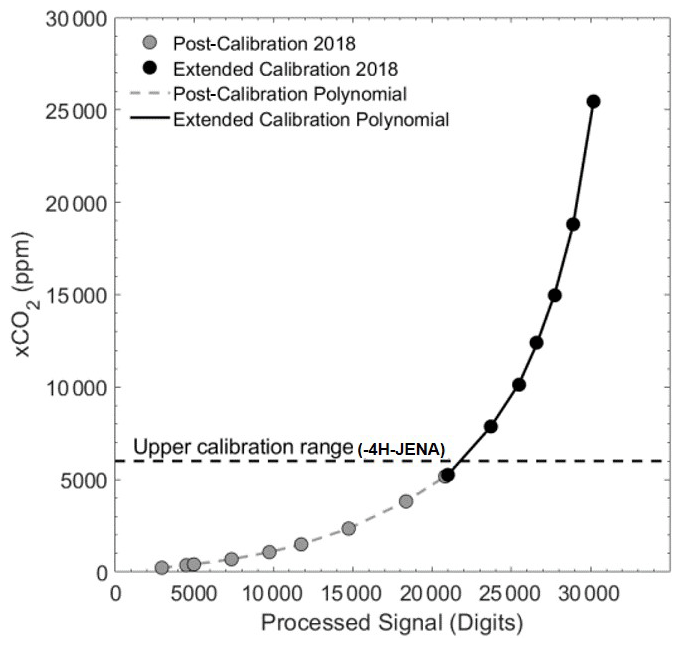
Figure 4 Calibration polynomial from the post-cruise manufacturer calibration (grey dots; KMCON) and the manual extended calibration curve (black dots), with the top range of the KMCON calibration range indicated (dashed line) above which the non-linear behaviour of the non-dispersive infrared (NDIR) spectrometry sensor becomes stronger. The processed signal was calculated from the raw and reference signal data during processing.

These modifications only affected the internal gas volume and flow properties to a small extent. An effect on the determined RT, compared to the RT of a standard HC–CH₄, is therefore considered negligible. This information was then applied to the raw HC–CH₄ field data, considering the measured flow rate and temperature and the method of (Fiedler et al., 2013).

Post-processing of the HC–O₂ followed the SOP provided by KMCON, using Garcia and Gordon (1992) combined fit constants. Further processing to convert the output into gravimetric (µmol kg⁻¹) and volumetric units (µmol L⁻¹) for comparison with other sensors and the discrete samples is described in the SCOR WG142 recommendations on O₂ quantity conversions (Bittig et al., 2018a). During the oceanic cruise, an average offset of $-\mathrm{19.04}\pm \mathrm{2.26}$ (± root mean square error – RMSE) µmol L⁻¹ and $-\mathrm{29.78}\pm \mathrm{5.04}$ (± RMSE) µmol L⁻¹ was also found within the open ocean and shelf, respectively, to discrete oxygen data. Two separate linear offset corrections were applied throughout all oceanic data. Significant optode sensor drift, particularly when the sensor is not in the water, is a well-documented phenomenon (Bittig et al., 2018b).

The output from the factory-calibrated SBE 45 thermosalinograph had no need for post-processing. All accuracies of the sensors are shown in Table 1.

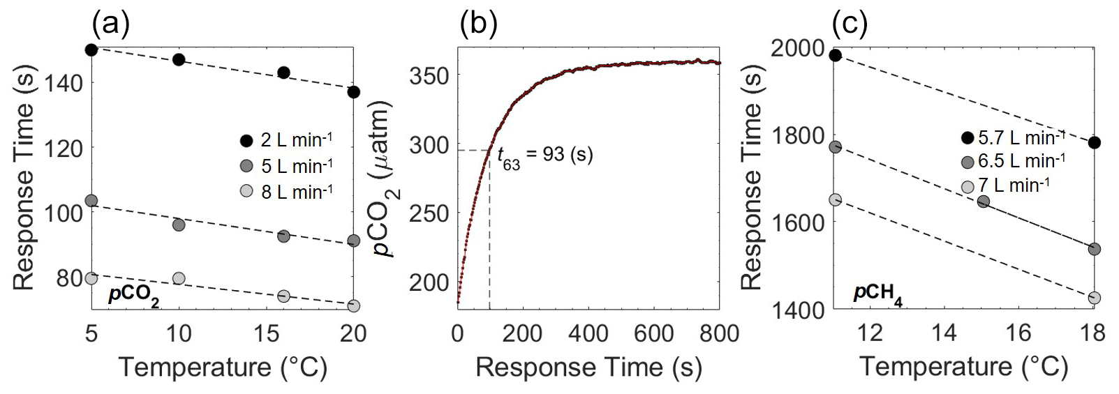
Figure 5 Response time (s) of the HC–CO₂ determined at four temperatures within controlled laboratory conditions for different water flow rates (2, 5 and 8 L min⁻¹) with errors too small to see (a). An example of the output (b) shows how t₆₃ is retrieved after a zeroing interval, with t₆₃ determined by the model's fit (line in red). Response time (RT) for pCH₄ is also shown (c) for flow rates of 5.7, 6.5 and 7 L min⁻¹ conducted in controlled conditions at KMCON.

3 Results

The set-up was easily adapted to each power source, managing to measure across the range of salinities and concentrations (Table 2). The results of the corrections are shown in the following sections.

Table 2 Cruise table for all field campaigns in 2016 and 2017, with cruise/ship names (cruise ID in italic), areas and observed maximum to minimum values for all measured parameters (in italic). For pCO₂, the sensor is only factory calibrated up to 6000 ppm; therefore, this was deemed as being the maximum in these circumstances.

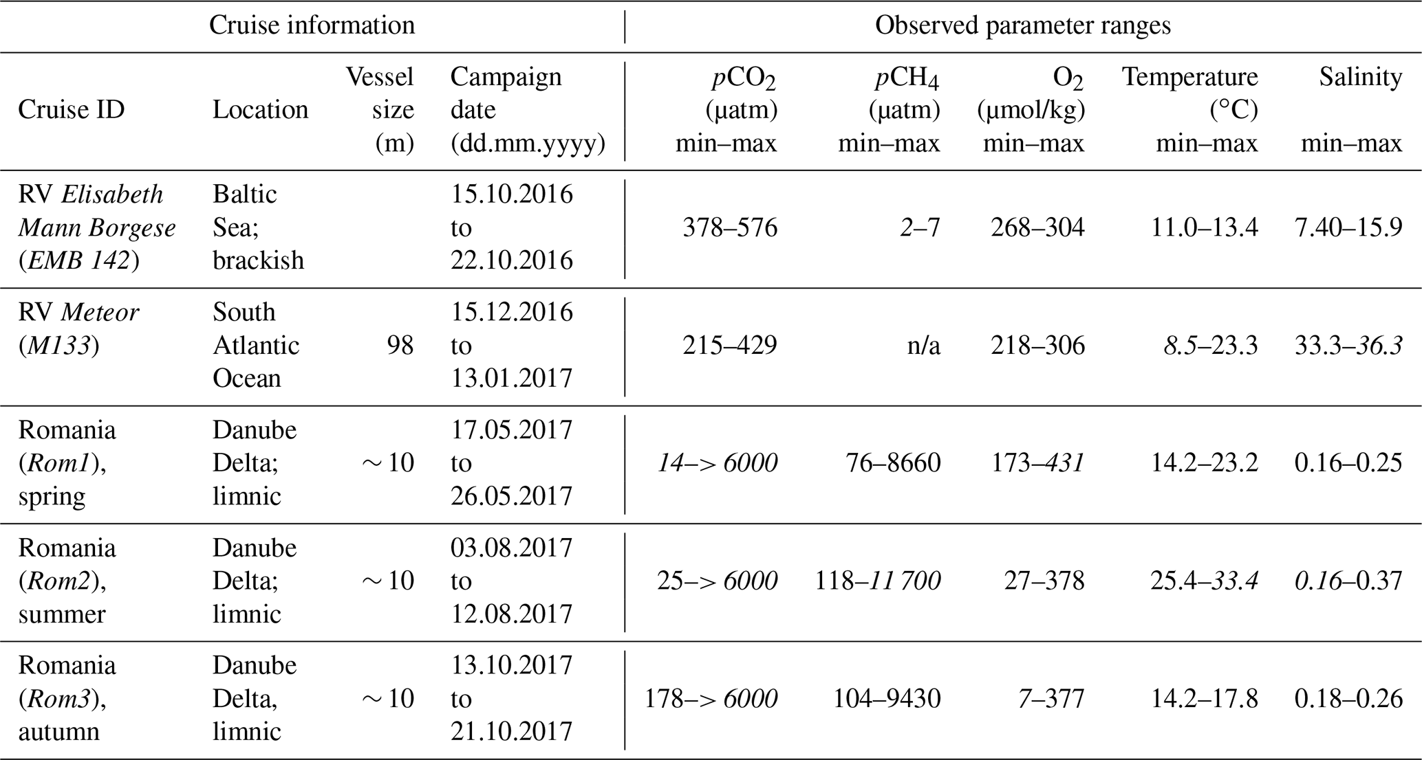
n/a: not applicable.

Figure 6 Section of a 24 h cycle of data from the autumn limnic cruise (Rom3), showing raw (black dashed line) and RT-Corr (black solid line) pCH₄ µatm measured by the HC–CH₄ with inverted pO₂ mbar (grey line) as a technically independent, yet parameter-wise, linked reference for real-time spatiotemporal variability, i.e. RT O₂ sensor ≪ RT CH₄ sensor.

3.1 Extended calibration

Compared with the prior calibration curve from the conducted calibration at KMCON, the final extended 5^∘ polynomial had to be shifted slightly (690 ppm). This was expected due to slightly different calibration methods and was done so that both polynomials matched at the top of the calibration range from KMCON (∼ 6000 ppm). The sensor was able to reach values of nearly 30 000 ppm before starting to reach saturation (Fig. 4). Given that this range was of similar magnitude to discrete samples and previous pCO₂ data from the Danube Delta (Marie-Sophie Maier, unpublished data; reaching values of up to and over 20 000 ppm), the correction was applied to all data above 6000 ppm. However, note that the general uncertainty of the sensor at this range is larger than that at company operational values, and due to the longer time period between deployments, spring and summer campaigns have an unquantified increased error. We assume 3 % as a conservative estimate of the overall accuracy of the xCO₂ measurements in the extended range (> 6000 ppm). From the noise of the signal during the calibrations, the estimated precision is ±1 % of the CO₂ reading, and we think that, even at this reduced accuracy, the observations in the high pCO₂ range are of significant scientific value.

3.2 RT correction analysis

The HC–CO₂ response time correction (RT-Corr) laboratory experiments quantitatively show the effect of temperature and flow and point to the importance of recording the flow data (Fig. 5). As stated before, due to varying flow and temperature, the HC–CO₂ RT was determined by the laboratory experiments shown in Fig. 5a. An example of the estimation of t₆₃ is given in Fig. 5b, which shows the signal recovery following a zeroing procedure, with t₆₃ = 93 s. Both increased flow rate and temperature reduce the RT of the sensor significantly.

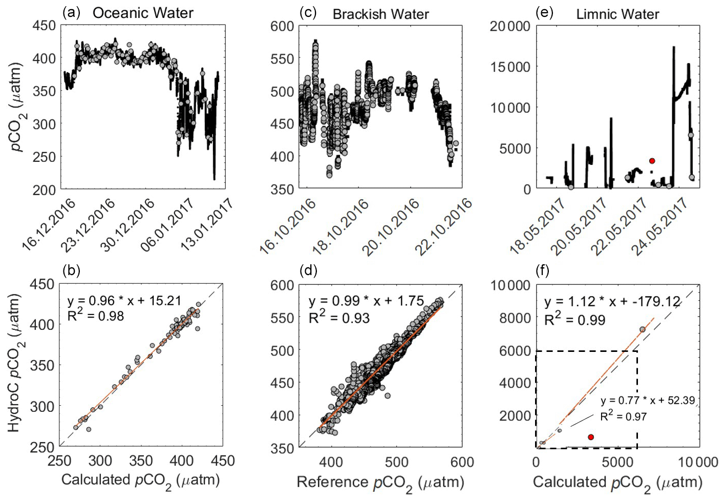
Figure 7 pCO₂ (µatm) from the HC–CO₂ within the following three regions: oceanic (a and b, including the open ocean and the Patagonian Shelf), brackish (c, d) and limnic waters (e, f) with the reference data used. The top graphs show the overall transects, with HC–CO₂ data as a black line and the reference data as grey dots (date presented as dd.mm.yyyy). The lower graphs are property–property plots showing the 1:1 line (dashed) and the line of the best linear fit (orange). For the validation of our system, we used the calculated pCO₂ from TA and DIC, using CO₂SYS for both oceanic and limnic waters, whereas a reference system was used for the brackish waters, as described above. During the Rom1 (limnic cruise), n=7 with the outlier in red (sample with an unclear match to flow-through data excluded from fit), with the box (dashed line) indicating the 6000 ppm company calibration limit.

The RT of the HC–CH₄ was far higher than for CO₂ and varied between 1425 and 1980 s (Fig. 5c), depending on temperature and flow, with both higher temperature and flow rate yielding shorter RT (for comparison, t₉₀ for the HC–CO₂ and HC–CH₄ was 212 and 3145 s, respectively). This was then applied to the raw HC–CH₄ data and compared with the pO₂, which has a RT of <3 s (KMCON; HydroFlash user manual) and therefore does not require an RT correction, to qualitatively assess the suitability of the correction, which can be seen from the near-perfect qualitative match between pCH₄ and pO₂ (Fig. 6). Note the inverted pO₂ due to typically having an inverse relationship with pCH₄.

3.3 Verification by discrete sample comparison

3.3.1 CO₂

Discrete pCO₂ was calculated from TA and DIC measurements that had an average precision from replicates of 1.48 µmol kg⁻¹ (TA) and 1.04 µmol kg⁻¹ (DIC) after the removal of one outlier sample. During the oceanic cruise, this provided a mean difference within the open ocean of $-\mathrm{0.13}\pm \mathrm{5.25}$ µatm (± SD) to the data measured by the HC–CO₂ flow-through system (HC–CO₂ pCO₂ – calculated pCO₂; DIC and TA). This mean increased within the productive waters along the Patagonia Shelf to up to 2.56±6.21 µatm (± SD). A comparison between the performances of the HC–CO₂ is shown in Fig. 7, where each region has been separated. The comparison for the brackish water is against the calibrated data from the state-of-the-art equilibrator set-up, using an LGR off-axis ICOS (Gülzow et al., 2011) showing an offset of $-\mathrm{2.87}\pm \mathrm{7.71}$ (± SD) µatm (HC–CO₂ – reference pCO₂). Note the change in pCO₂ for each region, varying from undersaturated (mainly oceanic waters) to supersaturated (brackish waters) and almost 20 000 µatm within the limnic waters during Rom1 (Fig. 7).

The limnic measurements of TA and DIC had an average precision based on replicates of 1.03 and 0.27 µmol kg⁻¹ for TA and DIC, respectively.

3.3.2 CH₄

The average offset of the reference system to the HC–CH₄ during the first half of the brackish cruise was $-\mathrm{0.95}\pm \mathrm{0.19}$ (± SD) µatm for the RT-Corr pCH₄ data (Fig. 8). This gave an average offset within the manufacturer accuracy specification range of ± 2 µatm, with a mean offset of 0.79±0.64 (± SD) µatm. Both sensors showed the same variability and magnitude to one another, even with the offset (Fig. 8).

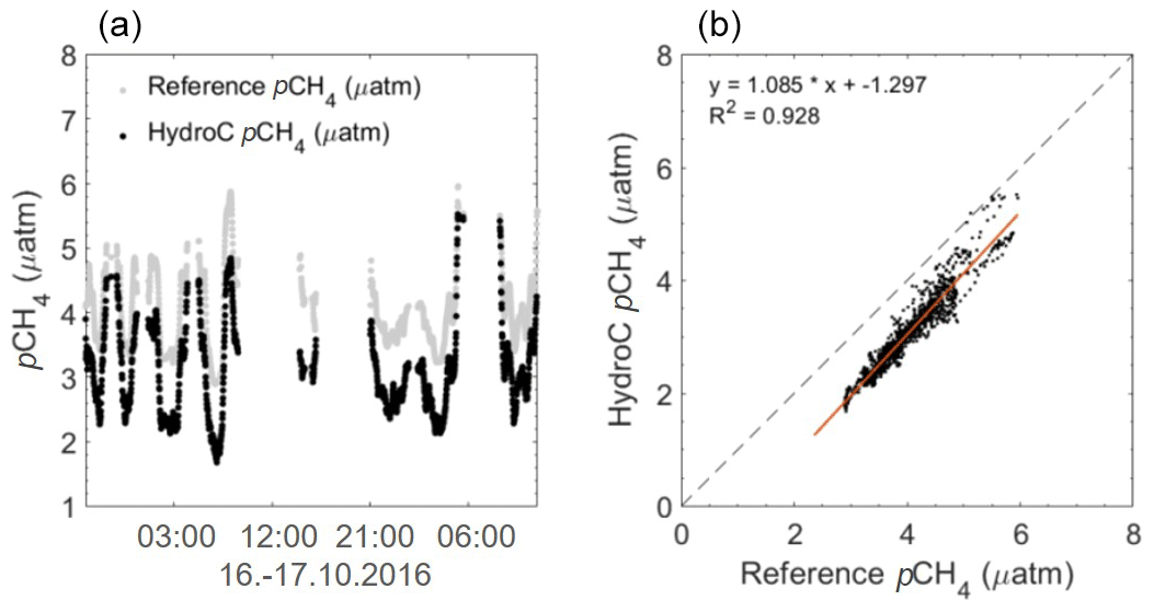
Figure 8 pCH₄ µatm data from the HC–CH₄ during the brackish cruise (EMB 142; RV Elisabeth Mann Borgese) expedition in the western Baltic Sea, with the reference system over the first half of the cruise. Panel (a) shows the HC–CH₄ data with a negative offset, resulting in lower concentrations compared to that of the reference data. Panel (b) shows a 1:1 plot, with a regression line (R²=0.928) illustrating the constant offset, but with a similar slope of data. Within the brackish waters, the offset was within the specifications from KMCON, yet both values (reference and HC–CH₄) were in the range of that previously found within the region (Gülzow et al., 2013).

Given the previous evaluation of the RT-Corr, this improved the accuracy of the HC–CH₄ within the limnic system of Romania (HC–CH₄ – measured pCH₄; Rom1 – from $-\mathrm{164.3}\pm \mathrm{1117.3}$ (± SD) µatm to 182.6±591.3 (± SD) µatm; Rom2 – from 609.3±1065 (± SD) µatm to 537.9 ± 1145 (± SD) µatm; Rom3 – from 466.5 ± 383 (± SD) µatm to 457.1 ± 376 (± SD) µatm; Rom1 is shown in Fig. 9). Matching discrete sample data with continuous sensor data that have a long RT becomes very complicated in highly variable situations. The effect of variable situations was also noticeable within the triplicates of the discrete samples, with some varying by over 400 µatm (with an average variability between repeated samples at 122.6 ± 100.9 (± SD) µatm), leading to the offset with the HC–CH₄ seeming reasonable. The agreement between sensor data and discrete samples increased significantly with the RT-Corr, as shown in Fig. 9, with the R² improving from 0.33 to 0.93 and the slope from 0.36 to 1.25. Peaks within the data are also observed within the discrete measurements (Fig. 9c) in combination with the sensor data, e.g. Fig. 9c between 20.05 and 21.05. It has to be noted that the determination of dissolved CH₄ concentrations from discrete samples is also not fully mature and shows significant inter-laboratory offsets (Wilson et al., 2018), and thus, the observed discrepancy is likely not to be entirely caused by our sensor-based measurements.

3.3.3 O₂

During the oceanic cruise, after the post-offset correction (stated above), O₂ µmol L⁻¹ had an average offset of −0.1 ± 3.4 (± SD) µmol L⁻¹ (HydroFlash O₂ – discrete samples O₂) over the whole transect (Fig. 10). Although stable and matching the variability throughout (Fig. 10a), note the increased offset observed when entering the Patagonian Shelf (Fig. 10b).

4 Discussion

We have presented a portable, easily accessible, quick to set up multi-gas measurement system that can autonomously measure across the entire LOAC. The operational boundaries of these sensors were tested over various deployment durations (∼ 1 month to hours), small spatial scales and under a wide range of operational environmental conditions.

Oceanic pCO₂ sensors are needed to operate with an overall accuracy of ± 2 µatm (Pierrot et al., 2009); therefore, this sensor performance throughout the open ocean was considered to be very good (Sect. 3.3.1). The offset found during the oceanic campaign, when entering the Patagonian Shelf (5.26 ± 4.33 µatm), is potentially due to biofouling within the tubing from the pump to the sensors. The offset observed by the optode for O₂ increased during the Patagonian Shelf waters due to the higher concentration ranges and gradients found along the shelf, possibly indicating an emerging biofouling issue of the sensor or within the casing surrounding the sensor. This demonstrated the overall relatively long-term stability and reliability of the O₂ optode even in an area with such extreme hydrographic variability. This was expected due to optodes being used widely in multiple environments (see Bittig et al., 2018b, Kokic et al., 2016, and Wikner et al., 2013, for oceanic, coastal and fresh water examples).

In the brackish water campaign, the HC–CO₂ and HC–CH₄ showed good agreement with the reference systems within the manufacturer's specifications. The data from the HC–CH₄, although having an internal issue as stated in Sect. 2.3.1, showed the same magnitude and variability as the reference system (Fig. 8). With little noise from both systems, natural variability was witnessed by both to further assure us that the system was running efficiently.

Figure 9 (a) Rom1 pCH₄ µatm data versus measured discrete samples of pCH₄ µatm, with both raw HC–CH₄ data and response time corrected (RT-Corr) data over the full range of concentrations. (b) A close-up view of the lower 800 µatm, with errors for the measured samples against the HC–CH₄ data. The grey line signals the line of best fit for the raw pCH₄, and the black line signals the RT-Corr pCH₄ µatm. (c) The full transect with discrete pCH₄ µatm samples for the spring cruise over time (date in dd.mm), but some error bars are too small to see.

The limnic campaigns were ideally suited to test the flexibility of these sensors, with concentration ranges reaching almost 30 000 µatm for pCO₂, over 10 000 µatm for pCH₄ and O₂ ranging from supersaturated to suboxic. Direct comparisons with the CH₄ and CO₂ concentrations show relatively similar variations to previous measurements within the Danube Delta lakes (Durisch-Kaiser et al., 2008; Pavel et al., 2009). Due to the design, physical placement and high flow speed, no biofouling of the membranes of the HC–CO₂ and HC–CH₄ occurred even within particle-rich environments, with very little settlement during our campaigns. However, our campaigns consisted of continuous movement through varying regions, and therefore, long-term stationary deployment in highly particulate waters may potentially lead to settlement. Overall, the set-up showed a good performance with continuous data collection, providing values within the expected ranges for pCO₂ across different salinity areas and when split into lakes rivers and channels (Hope et al., 1996; Bouillon et al., 2007; Lynch et al., 2010). However, in comparison to rivers and streams of a similar size, pCH₄ determined in this study generally had higher overall concentrations (Wang et al., 2009; Crawford et al., 2017) and higher overall medians (Stanley et al., 2016). Yet, they are within the range found for other freshwater systems and on a similar scale with other regions, showing large increases in CH₄ concentrations (Bange et al., 2019). When focusing on the discrete sample comparison between the calculated pCO₂ (from TA and DIC) and measured pCO₂ (HC–CO₂) in the limnic cruise (Sect. 3.3.1), the deviation was not unexpected due to the likely presence of organic alkalinity that causes an unknown TA bias leading to an offset in the calculated pCO₂ (Abril et al., 2015).

Having the combination of all these sensors, especially with CH₄, makes this set-up more unique for measurements across the LOAC. Due to the high accuracy needed for oceanic pCO₂ measurements, optimization and continuous improvements of these measurements has been occurring for decades (Körtzinger et al., 1996; Dickson et al., 2007; Pierrot et al., 2009) yet for a comparatively narrow range of oceanic conditions. Sensors have undergone multiple developments and improvements over these years, with the focus on measurements within these water bodies with high accuracy for a relatively small concentration range. In the market, there are currently few oceanic pCO₂ sensors capable of measuring under environmental conditions that cross the boundaries from limnic to oceanic, including the SAMI-CO₂ ocean CO₂ sensor (Sunburst Sensors, LLC, Missoula, MT, USA; see DeGranpre et al., 1995; Baehr and DeGrandpre, 2004; and Phillips et al., 2015). However, with similar accuracies in the ocean, one advantage of the continuous NDIR/TDLAS-based instruments used here is that no chemical consumables are required for the measurements (refer to the review papers for a discussion of different sensors, i.e. Clarke et al., 2017, and Martz et al., 2015, and for current technological updates on carbonate chemistry instrumentation, refer to the International Ocean Carbon Coordination Project, IOCCP, at http://www.ioccp.org/, last access: 30 October 2020). Traditional flow-through systems, on the other hand, such as the commonly used GO system (General Oceanics, Miami, FL, USA), are generally larger, more complex and built from more components. They also require more maintenance (see reference gases), and the data acquisition is therefore more labour-intensive, also increasing the probability of human error. Sensors designed for inland water bodies tend to be on the lower price range for various reasons, which unfortunately leads to lower accuracies and greater inconsistencies (Meinson et al., 2016; Friedlingstein et al., 2019; Canning, 2020). Measurements across the LOAC need high-accuracy sensors as the concentrations and dynamic ranges usually decrease from inland waters to the ocean and, thus, have to match with the oceanic standards, and the set-up presented here was designed to fulfil these requirements.

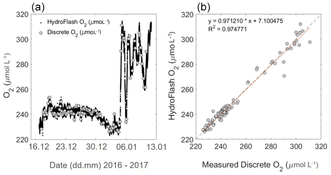
Figure 10 Oxygen concentration during cruise M133 from recalibrated continuous optode and discrete Winkler titration measurements (a) and a property–property plot (b). For the open ocean and shelf waters, the mean offset is −0.08 ± 1.89 (± SD) µmol L⁻¹ and −0.15 ± 6.49 (± SD) µmol L⁻¹, respectively. Higher variability towards the end of the transect is due to entering the productive Patagonian Shelf (06.01.2017–13.01.2017), which is also seen in higher concentrations of O₂.

Due to the higher quantity and quality of temporal and spatial measurements needed (Natchimuthu et al., 2017), below we present data examples from our various field campaigns to illustrate the utility and observational power of our approach to resolving both spatial and temporal variability in parallel for all measured quantities and at a very high resolution.

4.1 Temporal variability

In the Danube Delta, the portability of the set-up allowed us to focus on temporal variability for specific regions over three seasons. Due to the low power consumption, the small generator and car batteries were sufficient to easily run the entire set-up, allowing for high-resolution (up to 1 Hz), continuous measurements to extract diel cycles in the same way over the three seasons. Figure 11 displays data from a 2-week field campaign (Rom3), with areas of stationary measurements over extended time periods (grey shading in Fig. 11; see Fig. 3c for locations). Data were continuously logged for all parameters throughout the campaigns, with interruptions only when the houseboat docked. During each campaign, temporal variability showed differences between the regions (lakes, rivers and channels). The stationary phase of the first campaign was in a channel next to Lake Isaac (Fig. 11; grey box on 16.10.; duration 15 h:26 min; Fig. 3c1). An instant peak in CO₂ and CH₄ can be seen when entering the channel from the lake, coinciding with a drop in O₂. Over this diel cycle, CO₂ and O₂ are apparently governed by production and respiration, as expected (Nimick et al., 2011), yet with relatively constant and high CH₄ concentrations. However, during the second stationary zone measurements (Figs. 11; 3c2; 19.10.) conducted within a lake, pCO₂ is shown to increase steadily during the station, while always remaining far lower than within the channel. The same diel pattern is shown in the final station's stationary phase (Figs. 11; 3c4; 23.10.), which is located in one of the northern channels, far from any lake. These comparisons (from channel to lake variabilities) throughout the transects show the temporal variabilities within regions adjacent to, or within close proximity to, one another and differ vastly in both magnitude and diel pattern, even when comparing the same region (channel next to a lake – 16.10.; a further northern channel – 23.10.; Figs. 11; 3c4).

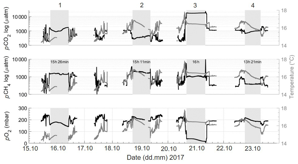
Figure 11 Sections acquired during the autumn limnic cruise. Rom3, showing pCO₂ (µatm; logarithmic scale), pCH₄ (µatm; logarithmic scale) and pO₂ (in mbar) and temperature (in ^∘C; grey) from the SBE across the entire deployment. Temperature is kept constant on the right y axis for direct changes to be noticed within each gas. Shaded areas and numbers (1–4) indicate periods of stationary observations when anchored in one location (see Fig. 3c1–4), with the station keeping durations in hours and minutes (shown in the middle row). Gaps in data collection refer to times when the systems were switched off.

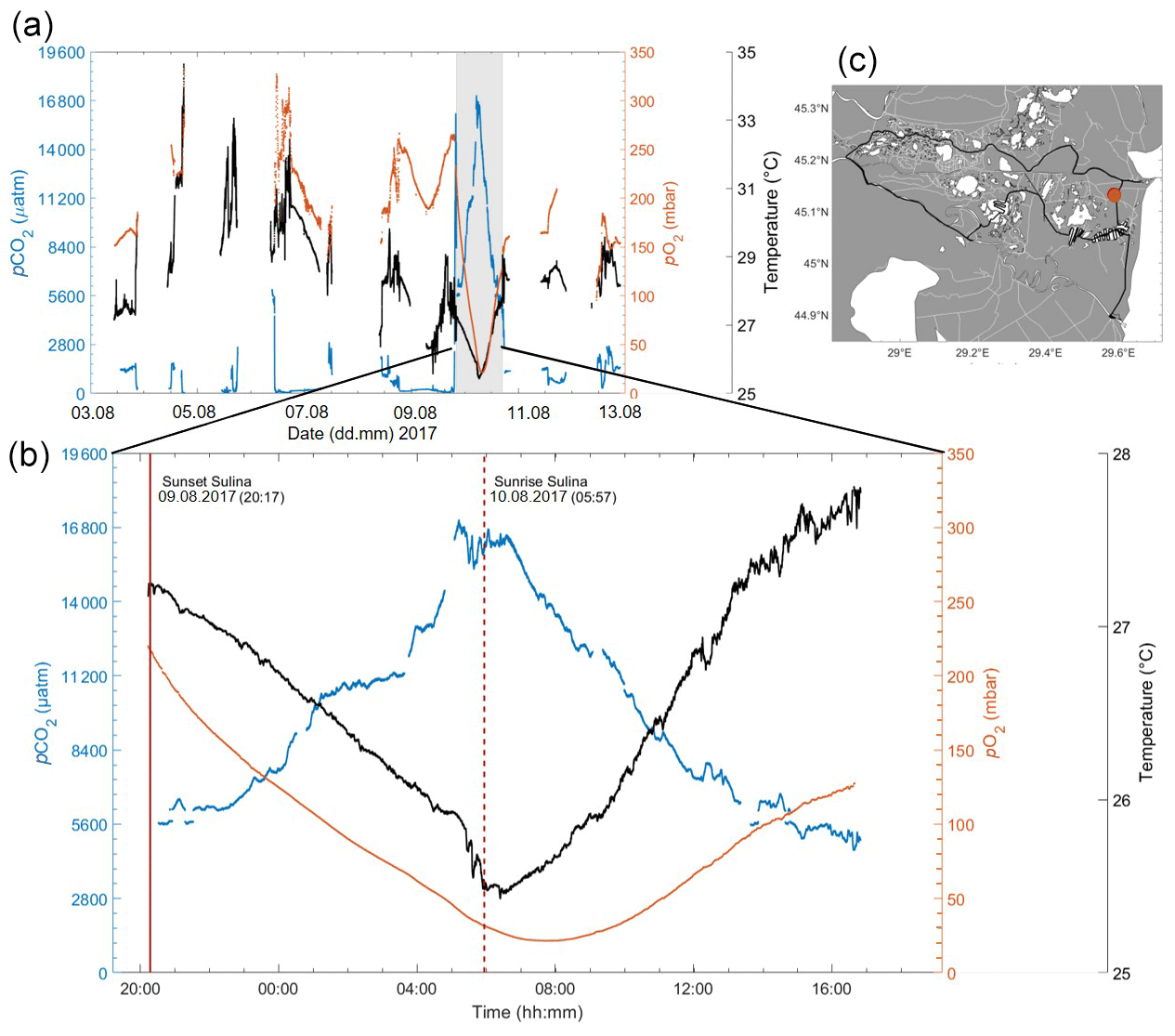
Figure 12 (a) Measurements of pCO₂ (in µatm; blue), pO₂ (in mbar; orange) and temperature (in ^∘C; black), during the Danube river campaign, Rom2, in summer 2017. The grey rectangle highlights a 24 h cycle acquired at a fixed location in a channel. (b) Close up of this 24 h cycle, with sunset (solid red) and sunrise (dashed line red) indicated, showing extreme variability in the diel cycle timescale. (c) Cruise track of the campaign, with the red dot indicating the position of the 24 h stationary data acquisition.

Looking closer into specific temporal variabilities, Fig. 12 shows an exemplary 24 h cycle within a small channel. This location was marked as a hotspot within our transect, showing drastic concentration changes with clear coupling between O₂, pCO₂ and temperature. The pCO₂ increases from 5000 µatm to nearly 17 000 µatm during the night, then decreases back to initial levels during the day, coinciding with sunrise and sunset, while the opposite trend for both temperature and pO₂ was observed. Timing and amplitude of these diel trends could have been lost with discrete sampling alone. Due to the same diel variation observed from this location over 2 of the 3 months (Rom1–2), uncertainties behind this variation, such as passing of water parcels anomalies or wind-driven variation as suggested before (Serra and Colomer, 2007; Van de Bogert et al., 2012), can be ruled out as possible explanations. Although diel cycles in inland waters have been investigated (for channels, estuarine, lakes and pond investigations, respectively; see Nimick et al., 2011; Maher et al., 2015; Andersen et al., 2017; van Bergen et al., 2019; Canning et al., 2020b), they are generally left out when it comes to average concentrations and corresponding fluxes. Evaluating our data gives evidence that such practices have to be critically evaluated, especially given the abundance and magnitude of diel cycles observed in these regions. Furthermore, allowing for multiple gases to be measured simultaneously enables extreme observations, such as this, to shed some light on the processes involved (Canning et al., 2020b). Therefore, any study aiming to measure representative concentrations and fluxes for limnic systems with significant diel variability will have to address this. Adequate sampling/observation schemes should be implemented to avoid strong biases (e.g. by both day–night sampling or by convoluting spatial and temporal variability in 24 h non-stationary mapping exercises).

4.2 Spatial variability

During the limnic campaigns, CH₄ showed extreme spatial and temporal differences, which highlight the need for high spatiotempral coverage. Although RT-Corr is not a new method within the ocean/brackish waters (see e.g. Fiedler et al., 2013; Gülzow et al., 2011; Miloshevich et al., 2004), the results of both the HC–CO₂ and HC–CH₄ corrections show high promise and an absolute need for such sensors in freshwaters that measure in highly spatially diverse regions. Both system stability and sensitivity could be demonstrated during the oceanic cruise (15 December 2016–13 January 2017; Fig. 13). A little spatial variability was expected over the large distance when crossing the open ocean waters of the South Atlantic Gyre. The fact that even these small variations in pCO₂, O₂ and temperature still show clear correlations points at the very low noise level of the measurements. The Brazil and Malvinas currents merge when entering the Patagonian Shelf, creating upwelling with fresh nutrients and, therefore, strongly increased primary production (Matano et al., 2010). These waters are characterized by high productivity with higher pO₂ and lower pCO₂ (Fig. 13) and increased overall variability compared to the open ocean. Some of these variabilities show the dynamic mixing between the contrasting water masses of the confluent surface currents. This region is one of the most productive and energetic regions throughout the ocean and is generally poorly described within models due to such dynamics (Arruda et al., 2015). The area is therefore an ideal location for demonstrating the high spatiotemporal resolution of our continuous, automatic multi-parameter approach.

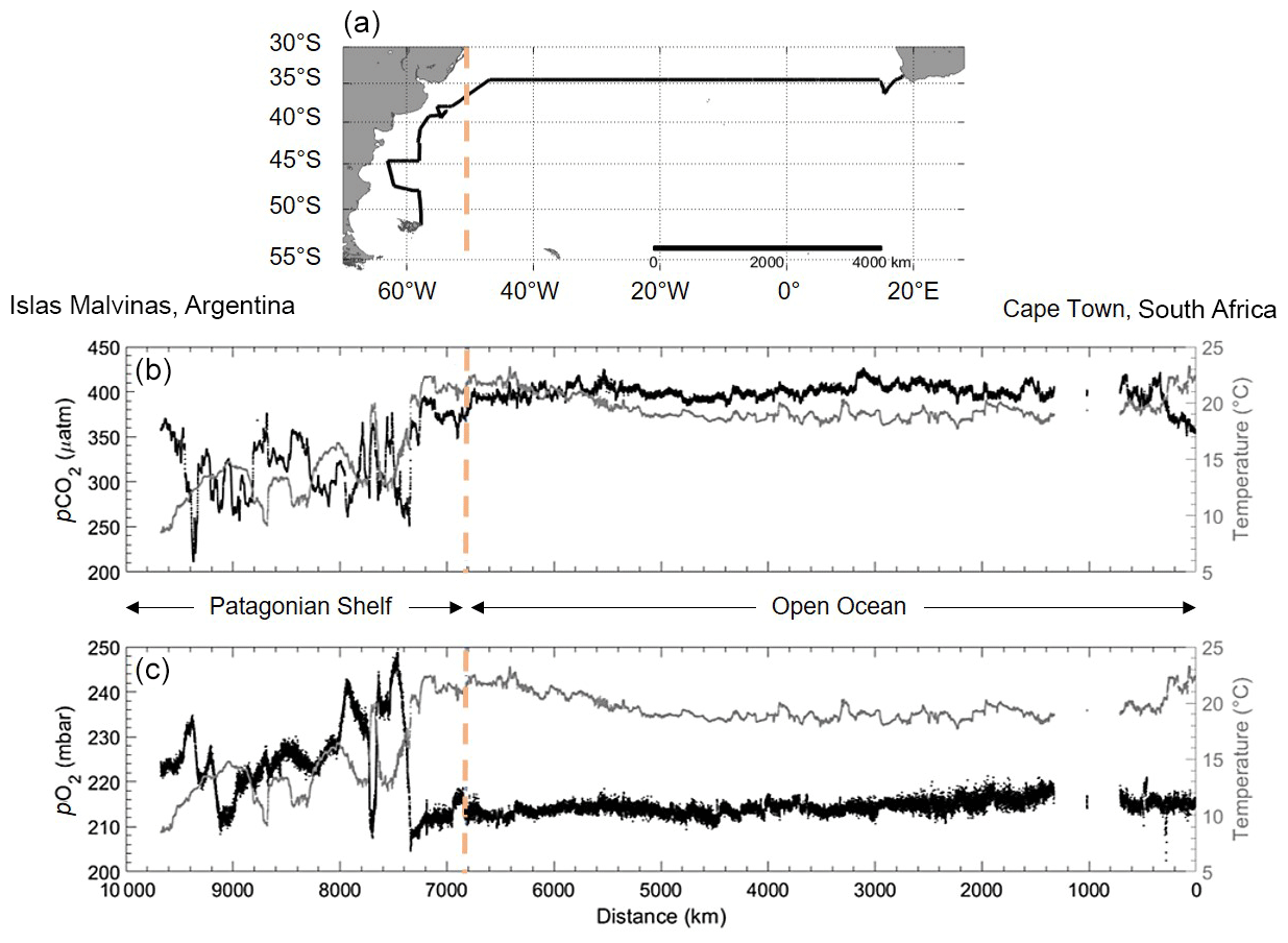
Figure 13 Data from the RV Meteor cruise M133 across the Atlantic Ocean (Cape Town, South Africa, to Islas Malvinas, Argentina). (a) Map of the cruise track (black line) across the Atlantic Ocean. The orange line shows the start of the cruise track entering the Patagonian Shelf. (b) pCO₂ (in µatm; black points) and (c) pO₂ (in mbar; black points), with water temperature (in ^∘C; grey line). Note the inverted x axis that coincides with the direction on the map. The Patagonian Shelf area (left of the orange dashed line) and open ocean (right of the orange dashed line) are also indicated.

In contrast to the utility for reliably mapping vast ocean regions, Rom1–3 enabled us to observe very small-scale spatial variability. Channels were noticeably playing a part in the spatial distribution of high pCO₂ and pCH₄ throughout the Danube Delta, as was true for most freshwater areas (Crawford et al., 2017). This is clearly observed during mapping of the St George river branch (Fig. 14). Although the variability in pCO₂ is relatively small (∼ ± 60 µatm), the higher concentrations are still picked up and seen to originate from a side channel, dispersing down the river branch. Although expected, due to the real-time measurement visualization by the CONTROS DETECT software, spatial impacts from the channels within more sensitive regions were immediately noticed, allowing for data-guided mapping. The versatility enabled us to complete small spatial-scale transects, with repetitions over time to ensure the concentration changes were primarily due to spatial and not temporal variability (see multiple transects in Fig. 14). This enables spatial dispersion distances to be measured on such small scales.

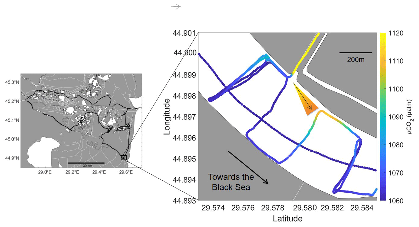
Figure 14 Small-scale spatial variability in pCO₂ (µatm) recorded in the Danube Delta from our river transects next to the entrance of a channel near St George. The direction of the water flow was visible, even with small changes in concentrations (arrow and interpretation of concentration gradient and flow direction is indicated to support the interpretation).

In more extreme cases, small-scale spatial changes were observed in areas of channels joining during Rom3, where the pCO₂ values decreased from 14 722 to 1623 µatm in just over 4 min (Fig. 15). With the houseboat travelling between 2–3 knots, this corresponds to a distance of about 400 m (Fig. 15). This change was detected within an artificial channel joining Lake Roşulette towards the Sulina river branch, arriving from the highest pCO₂ and pCH₄, along with the lowest O₂, throughout the delta transect (pCO₂ indicated on the map in Fig. 15). Also shown in Fig. 15 is the processed and the raw output from the HC–CO₂ (orange dashed), exemplifying the need for all corrections and post-processing steps described above to fully reveal the true spatial distribution. Hotspots and areas of spatially extreme dynamics could be easily passed over with discrete or intermediate sampling. Therefore, this ability to gather such data allows for better classification of individual systems.

Although not shown here, even concentration fluctuations due to vessels passing by were picked up immediately within the data, usually leading to increasing CO₂ and CH₄ concentrations. With recreational activities and boat usage within some regimes increasing, this should be considered when measuring both fluxes and overall concentrations.

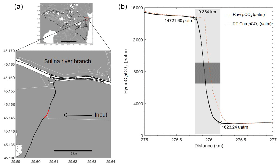
Figure 15 Extreme pCO₂ concentration gradient over a short time period (∼ 4 min indicated by the red line on the map in panel a and a light grey box on the graph in panel b) during Rom3. Raw pCO₂ (orange dashed line), compared with post-processed, response-time-corrected (RT-Corr) pCO₂ data (black), improving the spatial allocation of the gradient region by ∼ 100 m. The gradient occurred over a distance of about 400 m due to another channel providing a different water source (white lines indicating the channel). The dark grey box symbolizes the area over the concentration change in which the houseboat passed the entrance of the entering channel.

4.3 Limitations and benefits

As we have shown, this set-up can be used in the most variable of environments, picking up small variabilities and allowing for meter by meter readings. The benefit of the system being built for oceanic precision on the lower concentrations allows for the system to be continuously used over the boundaries of the LOAC. However, limitations of the system, such as the potential power supply for certain deployments and the long response time (which has been shown to be overcome by the application of the RT correction), are outweighed by the benefits of such a system, i.e. relatively long-term stability, reduced demand of human effort required compared to other systems and being able to pick up small variabilities with the response time correction (see Sect. 3.2). The system allows continuous measurements in combination with other parameters across all salinities and has a precision and accuracy acceptable for measurements in oceanic waters.

5 Conclusions

As one of the few studies to combine a sensor package across the entire LOAC for CO₂, CH₄ and O₂ measurements, the importance of seamless observations across the entire LOAC is becoming more apparent. Enabling and openly assessing a variety of techniques across all water types is essential for improving our understanding of carbon budgets and processes, especially within the inland regions. We have therefore tried to introduce oceanic precision and attention to detail into the field observations in inland water regions to potentially allow for measurements in regions of little to no data with a relatively cheap, fully enclosed sensor package with oceanic accuracy.

The results clearly demonstrate the observational power this technology can provide but, at the same time, illustrate the need for dedicated data processing addressing sensor issues (e.g. drift, calibration range and time constants) for the achievement of high data quality. Although all corrections were important, the RT-Corr for pCH₄ was viewed as vital when measuring in such a diverse regime (in inland waters), and therefore, such practices should be applied. The extended calibration laboratory experiments showed the ability to access higher concentration data values. Despite a slight increase in the error margin, these methods allow access to such high values with these sensors while keeping the precision of the lower concentrations. The results from the suite of campaigns presented here provide further evidence that techniques and sensors designed for specific regimes can be adapted and, when carefully assessed, provide precise measurements across boundaries and through highly diverse regions. This proves that oceanic sensors can be used across salinities in a portable way, with little attention needed during operation.

Improvements can be made in terms of size, individual placement of the sensors and accessibility; however, this set-up and data readings show the vitality of having high spatiotemporal resolution multi-gas data for mapping and diel cycle extraction, which can further assist with modelling efforts and assessing concentrations and fluxes (Canning et al., 2020b). Given that there is much need for both high spatial data coverage and accurate concentrations for inland CO₂ and CH₄ measurements (Crawford et al., 2014; Meinson et al., 2016; Yoon et al., 2016; Natchimuthu et al., 2017; Grinham et al., 2018), this type of data can help fill the gap in this specific region and/or mixing regimes. This can enable better classification of regions, thus furthering monitoring activities and overall carbon budget investigations which benefit from enhanced data acquisitions on higher spatial and temporal resolutions.

The main use of this continuous, high-resolution data can be split into the following four main sections: (a) large-scale monitoring and mapping efforts, (b) temporal variability observations (i.e., with observations in a fixed location or in Lagrangian perspective), (c) spatial variability observation (with a moving platform, often resulting in a convolution of spatial and temporal variability) and (d) the assessment of the coupling between the different continuously observed parameters. The use of separate techniques, from oceanography to limnology, is slowly becoming unnecessary, but there is a definite need for standardized corrections and post-processing in limnology, such as in the ocean.