the Creative Commons Attribution 4.0 License.
the Creative Commons Attribution 4.0 License.
 | 02 Mar 2021
Are there memory effects on greenhouse gas emissions (CO2, N2O and CH4) following grassland restoration?
Charlotte Decock
Werner Eugster
Kathrin Fuchs
Benjamin Wolf
Nina Buchmann
Lukas Hörtnagl
A 5-year greenhouse gas (GHG) exchange study of the three major gas species (CO2, CH4 and N2O) from an intensively managed permanent grassland in Switzerland is presented. Measurements comprise 2 years (2010 and 2011) of manual static chamber measurements of CH4 and N2O, 5 years of continuous eddy covariance (EC) measurements (CO2–H2O – 2010–2014), and 3 years (2012–2014) of EC measurement of CH4 and N2O. Intensive grassland management included both regular and sporadic management activities. Regular management practices encompassed mowing (three to five cuts per year) with subsequent organic fertilizer amendments and occasional grazing, whereas sporadic management activities comprised grazing or similar activities. The primary objective of our measurements was to compare pre-plowing to post-plowing GHG exchange and to identify potential memory effects of such a substantial disturbance on GHG exchange and carbon (C) and nitrogen (N) gains and losses. In order to include measurements carried out with different observation techniques, we tested two different measurement techniques jointly in 2013, namely the manual static chamber approach and the eddy covariance technique for N2O, to quantify the GHG exchange from the observed grassland site.
Our results showed that there were no memory effects on N2O and CH4 emissions after plowing, whereas the CO2 uptake of the site considerably increased when compared to pre-restoration years. In detail, we observed large losses of CO2 and N2O during the year of restoration. In contrast, the grassland acted as a carbon sink under usual management, i.e., the time periods 2010–2011 and 2013–2014. Enhanced emissions and emission peaks of N2O (defined as exceeding background emissions 0.21 ± 0.55 nmol m−2 s−1 (SE = 0.02) for at least 2 sequential days and the 7 d moving average exceeding background emissions) were observed for almost 7 continuous months after restoration as well as following organic fertilizer applications during all years. Net ecosystem exchange of CO2 (NEE) showed a common pattern of increased uptake of CO2 in spring and reduced uptake in late fall. NEE dropped to zero and became positive after each harvest event. Methane (CH4) exchange fluctuated around zero during all years. Overall, CH4 exchange was of negligible importance for both the GHG budget and the carbon budget of the site.
Our results stress the inclusion of grassland restoration events when providing cumulative sums of C sequestration potential and/or global warming potential (GWP). Consequently, this study further highlights the need for continuous long-term GHG exchange observations as well as for the implementation of our findings into biogeochemical process models to track potential GHG mitigation objectives as well as to predict future GHG emission scenarios reliably.
- Article
(2742 KB) - Full-text XML
-
Supplement
(202 KB) - BibTeX
- EndNote


Grassland ecosystems are commonly known for their provisioning of forage, either directly via grazing of animals on-site or indirectly by regular biomass harvest and preparation of silage or hay. Simultaneously, grasslands have further been acknowledged for their greenhouse gas (GHG) mitigation and soil carbon sequestration potential (Lal, 2004; Smith et al., 2008). However, greenhouse gas emissions from grasslands, particularly N2O and CH4, have been shown to offset net carbon dioxide equivalent (CO2 eq.) gains (Ammann et al., 2020; Dengel et al., 2011; Hörtnagl et al., 2018; Hörtnagl and Wohlfahrt, 2014; Merbold et al., 2014; Schulze et al., 2009). Still, datasets containing continuous measurements of all three major GHGs (CO2, CH4 and N2O) in grassland ecosystems remain limited (Hörtnagl et al., 2018), include a single GHG only, or focus on specific management activities (Fuchs et al., 2018; Krol et al., 2016). At the same time such datasets are extremely valuable by providing key training datasets for biogeochemical process models (Fuchs et al., 2020).
Here we investigate the GHG exchange of the three major trace gases (CO2, CH4 and N2O) over 5 consecutive years in a typical managed grassland on the Swiss plateau. Our study includes the application of traditional GHG chamber measurements and state-of-the-art GHG concentration measurements with a quantum cascade laser absorption spectrometer and a sonic anemometer in an eddy covariance setup (Eugster and Merbold, 2015). Prior to our measurements we hypothesized short-term losses of CO2 and more continuous losses of primarily N2O following dramatic managements events such as plowing occurring at irregular time intervals. We further hypothesized an increased carbon uptake strength compared to the pre-plowing years. Methane emissions were hypothesized to be of minor importance due to the limited time of grazing animals on-site (Merbold et al., 2014).
To date the majority of greenhouse gas exchange research has focused on CO2, with less focus on the other two important GHGs, N2O and CH4, even though an increased interest in these other gas species has become visible in recent years (Ammann et al., 2020; Ball et al., 1999; Cowan et al., 2016; Krol et al., 2016; Kroon et al., 2007, 2010; Necpálová et al., 2013; Rutledge et al., 2017). The existing exceptions are often referred to as “high-flux” ecosystems, namely wetlands and livestock production systems in terms of CH4 (Baldocchi et al., 2012; Felber et al., 2015; Laubach et al., 2016; Teh et al., 2011) and agricultural ecosystems such as bioenergy systems with considerable N2O emissions (Cowan et al., 2016; Fuchs et al., 2018; Krol et al., 2016; Skiba et al., 1996, 2013; Wecking et al., 2020; Zenone et al., 2016; Zona et al., 2013). Agricultural ecosystems and specifically grazed systems are characterized by GHG emissions caused through anthropogenic activities. These activities lead to changes in GHG emission patterns and include harvests; amendments of fertilizer and/or pesticides; and less frequently occurring plowing, harrowing and re-sowing events. While plowing has been shown to lead to considerable short-term emissions of CO2 and N2O (Buchen et al., 2017; Cowan et al., 2016; Hörtnagl et al., 2018; MacKenzie et al., 1997; Merbold et al., 2014; Rutledge et al., 2017; Vellinga et al., 2004), regular harvests have been shown to lead to increased CO2 uptake (Zeeman et al., 2010) and grazing leads to large CH4 emissions (Dengel et al., 2011; Felber et al., 2015). Other studies showed contrary results with reduced N2O emissions following plowing of a drained grassland when compared to a fallow in Canada (MacDonald et al., 2011).
Still, the full range of management activities occurring in intensively managed grasslands and their respective impact on GHG exchange has not been investigated in detail. In a recent synthesis including grasslands located along an altitudinal gradient in central Europe, Hörtnagl et al. (2018) highlighted the most important abiotic drivers of CO2 (light, water availability and temperature), CH4 (soil water content, temperature and grazing) and N2O (water-filled pore space and soil temperature) exchange. The study by Hörtnagl et al. (2018) further elaborated the variation in management intensity and related variations in GHG exchange across sites, stressing the need for more case studies based on continuous GHG observations to improve existing knowledge and close remaining knowledge gaps. To complete the picture on factors driving ecosystem GHG exchange, irregularly occurring events such as dry spells or extraordinary wet periods can further lead to enhanced or reduced GHG emissions (Chen et al., 2016; Hartmann and Niklaus, 2012; Hopkins and Del Prado, 2007; Mudge et al., 2011; Wolf et al., 2013).
While drought has been shown to reduce CO2 uptake in forests (Ciais et al., 2005) and dry spells have been shown to not affect CO2 uptake in grasslands (Wolf et al., 2013), flooding leads primarily to enhanced CH4 emissions (Knox et al., 2015) and large precipitation events can lead to plumes of N2O (Fuchs et al., 2018; Zona et al., 2013) similar to freeze–thaw events (Butterbach-Bahl et al., 2011; Matzner and Borken, 2008) to name only some examples. Consequently, understanding both anthropogenic impacts, such as management, and environmental impacts on ecosystem GHG exchange is crucially important to suggesting appropriate climate change mitigation as well as adaptation strategies for future land management with ongoing climate change.
Different measurement techniques to quantify the net GHG exchange in ecosystems are known, and the most common approach is either GHG chamber measurements or the eddy covariance (EC) technique. Static manual chamber measurements have been used for more than a century to quantify CO2 emissions (Lundegardh, 1927), and their application has been further expanded during the last few decades to quantify losses of the three major GHGs, CO2, N2O and CH4, from soils (Imer et al., 2013; Pavelka et al., 2018; Pumpanen et al., 2004; Rochette et al., 1997). Even though more complex in terms of technology and assumptions made before carrying out measurements, the eddy covariance (EC) technique has become a valuable tool to derive ecosystem-integrated CO2 and H2Ovapor exchange across the globe (Baldocchi, 2014; Eugster and Merbold, 2015). The technique has been further extended to continuous measurements of CH4 and N2O with the development of easy field-deployable fast-response analyzers during the last decade (Brümmer et al., 2017; Felber et al., 2015; Kroon et al., 2007; Nemitz et al., 2018; Wecking et al., 2020). Each of the two approaches has its strengths and weaknesses, and it is beyond the scope of this study to discuss each of them in detail. However, we refer to a set of reference papers highlighting the advantages and disadvantages of each technique separately: for chambers, see Ambus et al. (1993), Brümmer et al. (2017) and Pavelka et al. (2018); for eddy covariance, see Baldocchi (2014), Denmead (2008), Eugster and Merbold (2015), and Nemitz et al. (2018).
The overall objective of this study was to investigate the net GHG exchange (CO2, CH4 and N2O) before and after grassland restoration and thus fill existing knowledge gaps caused by limited numbers of available GHG exchange data from intensively managed grasslands. The specific goals were (i) to assess pre- and post-plowing GHG exchange in a permanent grassland in central Switzerland accounting for changes in GHG exchange following frequent management activities; (ii) to compare two different measurement techniques, namely eddy covariance and static greenhouse gas flux chambers, to quantify the GHG exchange in a business-as-usual year; and (iii) to provide a 5-year GHG budget of the site and quantify losses and gains of C and N. Based on our results we provide suggestions for future research approaches to further understand ecosystem GHG exchange, to mitigate GHG emissions and to ensure nutrient retention at the site for sustainable production from permanent grasslands in the future.
2.1 Study site
The Chamau grassland site (FLUXNET identifier – CH-Cha) is located in the pre-alpine lowlands of Switzerland at an altitude of 400 m a.s.l. (47∘12′37′′ N, 8∘24′38′′ E) and characterized by intensive management (Zeeman et al., 2010). The site is divided into two parcels (parcels A and B) with occasionally slightly different management regimes (see also Fuchs et al., 2018). Mean annual temperature (MAT) is 9.1 ∘C, and mean annual precipitation (MAP) is 1151 mm. The soil type is a Cambisol with a pH ranging between 5 and 6, a bulk density between 0.9 and 1.3 kg m−3, and a carbon stock of 55.5–69.4 t C ha−1 in the upper 20 cm of the soil. The common species composition consists of Italian ryegrass (Lolium multiflorum) and white clover (Trifolium repens L.). For more details of the site we refer to Zeeman et al. (2010).
CH-Cha is intensively managed, with activities being either recurrent – referred to as usual or regular – or sporadic. Usual management refers to regular mowing and subsequent organic fertilizer application in the form of liquid slurry (up to seven times per year). In addition, the site is occasionally grazed by sheep and cattle for a few days in early spring and/or fall (Hans-Rudolf Wettstein, personal communication, 2015, Table S1). Sporadic activities aim at maintaining the typical fodder species composition and comprise reseeding, herbicide and pesticide application, or irregular plowing and harrowing on an approximately decadal timescale (Merbold et al., 2014). By such activity, mice are eradicated and a high-quality sward for fodder production is re-established following weed contamination. Specific information on management activity (timing, type of management, amount of biomass harvested) was reported by the farmers on-site (Table S1). Additionally, representative samples of organic fertilizer were collected shortly before fertilizer application events and sent to a central laboratory for nutrient content analysis (Labor für Boden- und Umweltanalytik, Eric Schweizer AG, Thun, Switzerland). Harvest estimates were compared to estimates based on destructive sampling of randomly chosen plots (n = 10) in the years 2010, 2011, 2013 and 2014. The amount of harvested biomass in the year 2012 was based on a calibration of the values presented by the farmer in comparison to the on-site destructive harvests in previous and following years (Table S1).
2.2 Eddy covariance flux measurements
2.2.1 Eddy covariance setup
The specific site characteristics with two prevailing wind directions (north-northwest and south-southeast) allow continuous observations of both management parcels. It is noteworthy that the separation of the two parcels is made exactly at the location of the tower. See Zeeman et al. (2010) and Fuchs et al. (2018) for further details. The eddy covariance setup consisted of a three-dimensional sonic anemometer (2.4 m height; Solent R3, Gill Instruments, Lymington, UK), an open-path infrared gas analyzer (IRGA; LI-7500A, Li-Cor Biosciences, Lincoln, NE, USA) to measure the concentrations of CO2 and H2Ovapor, and a recently developed continuous-wave quantum cascade laser absorption spectrometer (mini QCLAS; CH4, N2O, H2O configuration; Aerodyne Research Inc., Billerica, MA, USA) to measure the concentrations of CH4, N2O and H2Ovapor. Three-dimensional wind components (u, v, w) and CO2 and H2Ovapor concentration data from the IRGA were collected at a 20 Hz time interval, whereas concentrations of CH4 and N2O were collected at a 10 Hz rate from the QCLAS. The QCLAS provided the dry mole fraction for both trace gases (CH4 and N2O), and data were transferred to the data acquisition system (Moxa embedded Linux computer; Moxa, Brea, CA, USA) via an RS-232 serial data link and merged with the sonic anemometer and IRGA data streams in near real time (Eugster and Plüss, 2010). Important to note is that the QCLAS was stored in a temperature-controlled box (temperature variation during the course of a single day was reduced to <2 K) and located approximately 4 m away from the EC tower to avoid long tubing. The total tube length from the inlet near the sonic anemometer to the measurement cell was 6.5 m. The inlet consisted of a coarse sinter filter (common fuel filter used in model cars) and a fine vortex filter (mesh size 0.3 µm and a water trap) installed directly in front of the QCLAS. Filters were changed monthly or if the cell pressure in the laser dropped by more than 2 Torr (266.6 Pa). A flow rate of approximately 15 L min−1 was achieved with a large vacuum pump (BOC Edwards XDS-35i, USA, and TriScroll 600, Varian Inc., USA – the latter was used during maintenance of the Edwards pump). The pumps were maintained annually and replaced twice due to malfunction during the observation period. The infrared gas analyzer was calibrated to known concentrations of CO2 and H2O each year. The QCLAS did not need calibration due to its operating principles, and an internal reference cell (mini-QCL manual, Aerodyne Research Inc., Billerica, MA, USA) eased finding the absorption spectra after each restart of the analyzer.
2.2.2 Eddy covariance flux processing, post-processing and quality control
Raw fluxes of CO2, CH4 and N2O (FGHG; µmol m−2 s−1) were calculated as the covariance between turbulent fluctuations in the vertical wind speed and the trace gas species mixing ratio, respectively (Baldocchi, 2003; Eugster and Merbold, 2015). Open-path infrared gas analyzer (IRGA) CO2 measurements were corrected for water vapor transfer effects (Webb et al., 1980). A two-dimensional coordinate rotation was performed to align the coordinate system with the mean wind streamlines so that the vertical wind vector w=0. Turbulent departures were calculated by Reynolds (block) averaging of 30 min data blocks. Frequency response corrections were applied to raw fluxes, accounting for high-pass and low-pass filtering for the CO2 signal based on the open-path IRGA as well as for the closed-path CH4 and N2O data (Fratini et al., 2014). All fluxes were calculated using the software EddyPro (version 6.0, Li-Cor Biosciences, Lincoln, NE, USA) (Fratini and Mauder, 2014).
The quality of half-hourly raw time series was assessed during flux calculations following Vickers and Mahrt (1997). Raw data were rejected if (a) spikes accounted for more than 1 % of the time series, (b) more than 10 % of available data points were significantly different from the overall trend in the 30 min time period, (c) raw data values were outside a plausible range (± 50 µmol m−2 s−1 for CO2, ± 300 nmol m−2 s−1 for N2O and ± 1 µmol m−2 s−1 for CH4) and (d) window dirtiness of the IRGA sensor exceeded 80 %. Only raw data that passed all quality tests were used for flux calculations.
Half-hourly flux data were rejected if (e) fluxes were outside a physically plausible range (i.e., ± 50 µmol m−2 s−1 for CO2), (f) the steady-state test exceeded 30 % and (g) the developed turbulent conditions test exceeded 30 % (Foken et al., 2004). Between 1 January 2010 and 31 December 2014 64 572 (88 % of all possible data) 30 min flux values were calculated for CO2, of which 42 865 (57.8 %) passed all quality tests and were used for analyses in the present study (Table 1). The number of available flux values for N2O and CH4 were fewer, since we were only capable to continuously measure both gases from 2012 onwards (Table 1). Flux values in this paper are given as number of moles of matter or mass per ground surface area and unit of time. Negative fluxes represent a flux of a specific gas species from the atmosphere into the ecosystem, whereas positive fluxes represent a net loss from the system.
Table 1Data availability of GHG fluxes measured over the 5-year observation period. Values are given as all data possible, raw processed values and high-quality (HQ) data for the chamber flux data if above the detection limit, which were then used in the analysis. Bold font values represent the time period when both methods (EC and static chambers) were used simultaneously to estimate . Static chamber flux data are further marked in italic font.
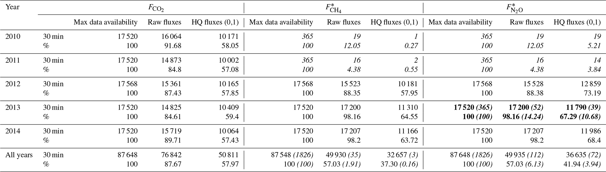
* Data availability in parentheses is based on static manual chambers (2010 and 2011, approx. biweekly measurements (n is 19 and 16, respectively; Imer et al., 2013), as well as during summer 2013 (n = 52)). High-quality data were only the data points that were above the minimum detection limits calculated. For further information see Sects. 2.3 and 4.1.
2.3 Static greenhouse gas flux chambers
2.3.1 Manual static GHG chamber setup
Static manual opaque GHG chambers were installed within the footprint of the site to measure soil fluxes in 2010 and 2011 (n = 16) as well as during summer 2013 (n = 10). The chambers were made of polyvinyl chloride tubes with a diameter of 0.3 m (Imer et al., 2013). The average headspace height was 0.136 m ± 0.015 m, and average insertion depth of the collars into the soil was 0.08 m ± 0.05 m. During sampling days with vegetation larger than 0.3 m inside the chamber, collar extensions (0.45 m) were used (2013 only). Chamber lids were equipped with reflective aluminum foil to minimize heating inside the chamber during the period of actual measurement. Spacing between the chambers was approximately 7 m, and an equal number of chambers were installed in each parcel. For further details we refer to Imer et al. (2013). Chamber measurements were carried out on a weekly basis during the growing season in all 3 years (2010, 2011 and 2013) and at least once a month during the winter season in 2010 and 2011. More frequent measurements of N2O emissions (every day) were performed following fertilization events in 2013 for 7 consecutive days after each event. Besides this, an intensive measurement campaign lasting 48 h (2 h measurement interval) was carried out in September 2010.
2.3.2 GHG concentrations measurements
During each chamber closure, four gas samples were taken, one immediately after closure and then in approximately 10 min time increments. With this approach, we guaranteed that the chambers were closed for no longer than 40 min to avoid potential saturation effects. Syringes (60 mL volume) were inserted into the chambers' lid septa to take the gas samples. The collected air sample was injected into pre-evacuated 12 mL vials (Labco Limited, Buckinghamshire, UK) in the next step. Prior to the second, third and fourth sampling of each chamber, the air in the chamber headspace was circulated with the syringe volume of air from the chamber headspace to minimize effects of built-up concentration gradients inside the chamber.
Gas samples were analyzed for their respective CO2, CH4 and N2O concentrations in the laboratory as soon as possible after sample collection and not stored for more than a few days. Gas sample analysis was performed with a gas chromatograph (Agilent 6890 equipped with a flame ionization detector, a methanizer – Agilent Technologies Inc., Santa Clara, USA – and an electron capture detector – SRI Instruments Europe GmbH, 53604 Bad Honnef, Germany) as described by Hartmann and Niklaus (2012).
2.3.3 GHG chamber flux calculations and quality control
GHG fluxes were calculated based on the rate of gas concentration change inside the chamber headspace. Data processing, which included flux calculation and quality checks, was carried out with the statistical software R (R Development Core Team, 2013). Thereby the rate of change was calculated by the slope of the linear regression of gas concentration over time. Flux calculation was based on the common equation containing GHG concentration (c in nmol mol−1 for CH4 and N2O), time (t in seconds), atmospheric pressure (p in Pa), the headspace volume (V in m−3), the universal gas constant (R = 8.3145 m−3 Pa K−1 mol−1), ambient air temperature (Ta in K) and the surface area enclosed by the chamber (A in m−2) (Eq. 1 in Imer et al., 2013).
Flux quality criteria were based on the fit of the linear regression. If the correlation coefficient of the linear regression (r2) was <0.8, the actual flux value was rejected from the subsequent data analysis (see Imer et al., 2013, and Table 1 for further details on data quality control). Furthermore, if the slope between the first and second GHG concentration measurement deviated considerably from the following concentrations, we omitted the first value and calculated the flux based on three instead of four samples. Mean chamber GHG fluxes were then calculated as the arithmetic mean of all available individual chamber fluxes for each date. A total of 35 GHG flux calculations (CH4 and N2O) were available for the years 2010 and 2011. Another 52 N2O flux values were available for the 5-month peak growing season in 2013.
2.4 Gap filling and annual sums of CO2, CH4 and N2O
To date a common strategy to fill gaps in EC data of CH4 and N2O has not been agreed on. The commonly used methods are simple linear approaches (Mishurov and Kiely, 2011) or the application of more sophisticated tools such as artificial neural networks (Dengel et al., 2011). The difficulty of finding an adequate gap-filling strategy results from the fact that emission pulses of either N2O or CH4 remain challenging to predict. Similarly, different measurement approaches – i.e., low-temporal-resolution manual GHG chambers compared to high-temporal-resolution eddy covariance measurements – need different gap-filling approaches (Mishurov and Kiely, 2011; Nemitz et al., 2018). In order to keep the gap-filling methods as simple and reliable as possible, we used a running median (30 and 60 d for eddy-covariance-based and chamber N2O fluxes, respectively). A similar approach was recently chosen by Hörtnagl et al. (2018) due to its reduced sensitivity to peaks in the N2O exchange data. The approach was particularly chosen as it minimizes the bias occurring from linear gap filling or simply using an overall average value. While the gap-filling approach may be of less importance for EC flux measurements with its high temporal data availability, it is the more important one for less frequently available GHG fluxes derived via manual chambers. Given the occurrence of sporadic N2O peaks which occur mostly in relation to management activities and last for a few hours or days only as well as the labor needed to carry out GHG chamber measurements, researchers commonly aim at having weekly or biweekly flux data (i.e., Imer et al., 2013). The respective sampling design is commonly designed to capture potential N2O flux peaks as well as some background values (Mishurov and Kiely, 2011). If one then uses either a linear interpolation or an overall average value, one can derive a budget which is than a likely overestimation of the annual flux budget caused by the few flux peaks observed in such managed systems. The same bias is likely to occur if just flux averages are used since few very high emission peaks will affect such an average. For this reason and in order to simulate N2O emission peaks more reliably, we have chosen the approach taken by Hörtnagl et al. (2018).
In contrast to CH4 and N2O, various well-established approaches to fill CO2 flux data gaps exist (Moffat et al., 2007). Here, we filled gaps in CO2 exchange data following the marginal-distribution sampling method (Reichstein et al., 2005) which was implemented in the R package REddyProc (https://r-forge.r-project.org/projects/reddyproc/, last access: 16 March 2016).
Calculation of the global warming potential (GWP) given in CO2 equivalents followed the recommendations given in the Fifth Assessment Report of the Intergovernmental Panel on Climate Change (IPCC), with CH4 having a 28 and N2O a 265 times greater GWP than CO2 on a per mass basis over a time horizon of 100 years (Stocker et al., 2013).
2.5 Meteorological and phenological data
Flux measurements were accompanied by standard meteorological measurements. These included observations of soil temperature (depths of 0.01, 0.02, 0.05, 0.10 and 0.15 m; TL107 sensors, Markasub AG, Olten, Switzerland), soil moisture (depths of 0.02 and 0.15 m; ML2x sensors, Delta-T Devices Ltd., Cambridge, UK) and air temperature (2 m height; HygroClip S3 sensor, Rotronic AG, Switzerland). Furthermore, we measured the radiation balance including shortwave incoming and outgoing radiation and longwave incoming and outgoing radiation (CNR1 sensor with ventilated Markasub housing, Kipp & Zonen, Delft, the Netherlands) as well as photosynthetically active radiation at 2 m height (PAR Lite sensor, Kipp & Zonen, Delft, the Netherlands). All data were stored as 30 min averages on a data logger in a climate-controlled box on-site (CR10X, Campbell Scientific, Logan, UT, USA).
3.1 General site conditions
The Chamau study site (CH-Cha) experienced meteorological conditions typical of the site during the 5-year observation period. Summer precipitation commonly exceeded winter precipitation (Fig. 1a). A spring drought was recorded from March till May 2011 (Wolf et al., 2013), leading to considerably lower soil water content than in previous and following years (Fig. 1a). Average daily air temperatures rose up to 26.7 ∘C (27 July 2013) during summer, and average daily temperature in winter dropped as low as −12.7 ∘C (6 February 2012, Fig. 1b) with soil temperature following in a dampened pattern (Fig. 1b). Average daily photosynthetic photon flux density did not differ considerably over the 5-year observation period (Fig. 1c). The site rarely experienced snow cover during winter (Fig. 1b).
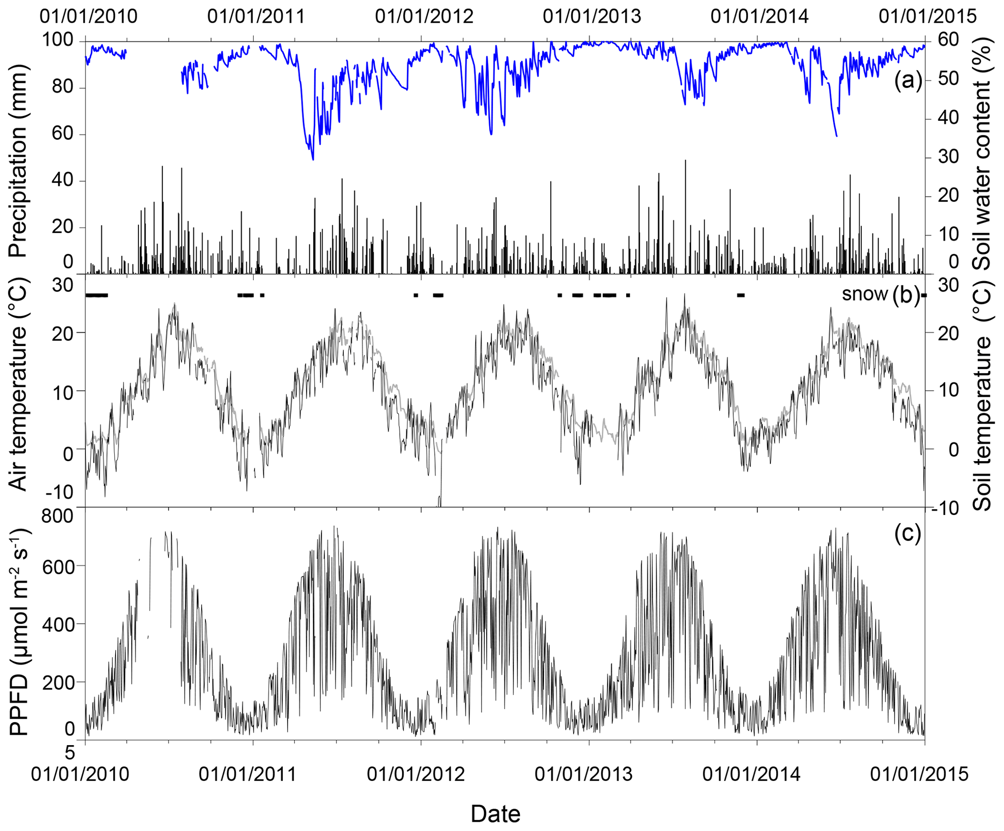
Figure 1Weather conditions during the years 2010–2014. Weather data were measured with our meteorological sensors installed on-site. (a) Daily sum of precipitation (mm) and soil water content (SWC, blue line, m3 m−3) measured at 5 cm soil depth; (b) daily averaged air temperature (∘C), daily averaged soil temperature (grey line, ∘C) and days with snow cover (horizontal bars); (c) daily averaged photosynthetic photon flux density (PPFD; µmol m−2 s−1). Days with snow cover were identified with albedo calculations. Days with albedo >0.45 were identified as days with either snow or hoarfrost cover.
The complexity in management activities becomes apparent when comparing business-as-usual years (e.g., 2011) with the restoration year (2012, Fig. 2a and b), highlighting the importance of grassland restoration to maintain productivity yields. Prior to 2012 an obvious decline in productivity with larger C and N inputs was found compared to the outputs in the years after restoration (2013 and 2014, Fig. 2a and b).

Figure 2Management activities for both parcels (A and B in panels a and b, respectively) on the CH-Cha site. Overall management varied particularly in 2010 between both parcels, whereas similar management took place between 2011 and 2014. Arrow direction indicates whether carbon (C in kg ha−1) and/or nitrogen (N in kg ha−1) was amended to or exported from the site (Fo and Fo∗ – organic fertilizers, slurry and manure (red); Fm – mineral fertilizer (light orange); H - harvest (light blue); Gs and Gc – grazing with sheep and cows, respectively (light and dark brown)). Other colored arrows visualize any other management activities such as pesticide application (Ph – herbicide (light pink); Pm – molluscicide (dark pink); T – tillage (black), R – rolling (light grey) and S – sowing (dark grey)) which occurred predominantly in 2010 (parcel B) and 2012 (parcels A and B). Carbon imports and exports are indicated by black and grey bars. Thereof black indicates the start of the specific management activities and grey the duration (e.g., during grazing, Gs). Green colors indicate nitrogen amendments or losses, with dark green visualizing the start of the activity and light green colors indicating the duration. Sign convention: positive values denote export or release and negative values import or uptake.
3.2 EC N2O fluxes vs. chamber-derived N2O fluxes
In 2013, we had the chance of comparing N2O fluxes measured with two considerably different GHG measurement techniques, namely eddy covariance and static chambers. The chambers (n = 10) were installed within the EC footprint. Our results reveal a similar temporal pattern, with increased N2O losses being captured by both methodologies following fertilizer application. However, we could not identify a consistent bias of either technique (Fig. 3a). Direct comparison of both measurements revealed a reasonable correlation (slope m= 0.61, r2=0.4) and larger variation between both techniques with increasing flux values (Fig. 3b).

Figure 3(a) Temporal dynamics of N2O fluxes measured with the eddy covariance (white circles) and manual greenhouse gas chambers (black circles measured in 2013) – grey lines indicate standard deviation. Arrows indicate management events (H – harvest, Fo – organic fertilizer application (slurry), Ph – pesticide (herbicide) application). (b) A 1:1 comparison between chamber-based and eddy-covariance-based N2O fluxes in 2013. The dashed line represents the 1:1 line (; r2=0.4; m=0.61; c=0.17; p<0.0001). Sign convention: positive values denote export or release and negative values import or uptake.
3.3 Temporal variation in GHG exchange
Fluxes of CO2 and N2O showed considerable variation between and within years. This variation primarily occurs due to management activities and seasonal changes in meteorological variables (Figs. 1 and 4). In contrast, methane fluxes did not show a distinct seasonal pattern.
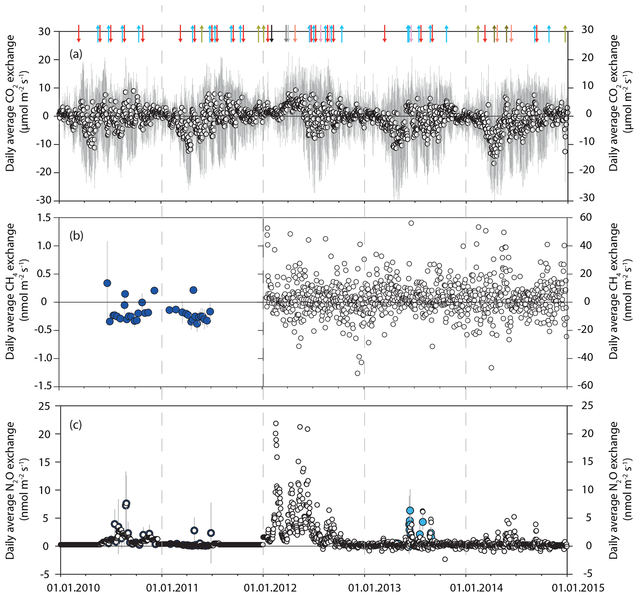
Figure 4Temporal dynamics of gap-filled (except methane in 2010–2011) daily averaged greenhouse gas (GHG) fluxes (white circles): (a) CO2 exchange in µmol m−2 s−1, (b) CH4 exchange in nmol m−2 s−1 and (c) N2O exchange in nmol m−2 s−1. Colored circles indicate manual chamber measurements. While both GHGs CH4 and N2O were measured in 2010 and 2011 (dark blue circles), only N2O was measured in 2013 (light blue circles). The dashed grey lines indicate the beginning of a new year. The same color coding as used in Fig. 3a is used to highlight management activities. Sign convention: positive values denote export or release and negative values import or uptake. Grey lines behind the circles indicate standard deviation.
3.3.1 CO2 exchange
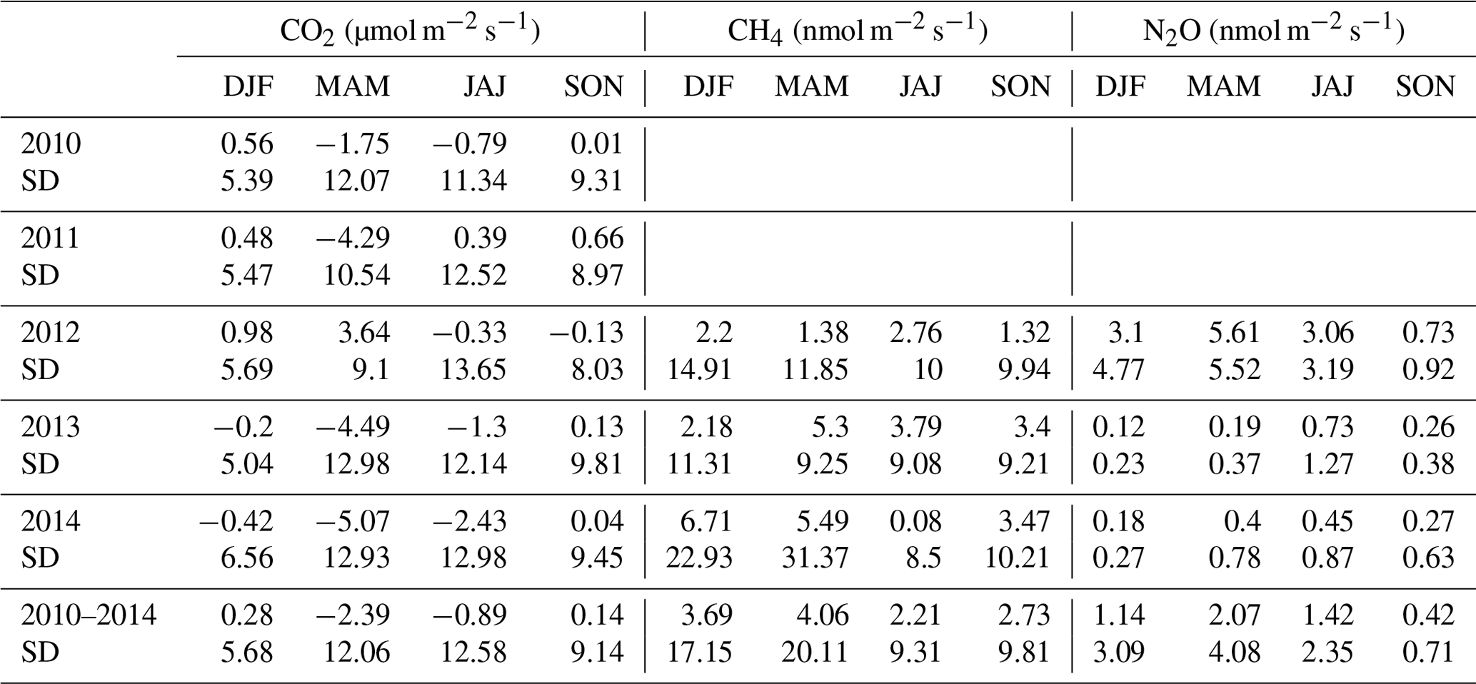
In pre-plowing years (2010 and 2011), the Chamau site showed 60 % lower CO2 uptake compared to the post-plowing years (2013 and 2014, Table 2). All 4 non-plowing years revealed the largest CO2 uptake rates in late spring (daily averaged peak uptake rates were >10 µmol CO2 m−2 s−1, March and April, Fig. 4a). Besides the seasonal effects a clear impact of harvest events could be identified, with abrupt changes from net uptake of CO2 to either reduced uptake or net loss of CO2 (light blue arrows indicate harvest event, Fig. 4a). A similar but less pronounced effect was found following grazing periods (light and dark brown arrows, Fig. 4a). A complete switch from net uptake to net CO2 release was observed during the first 3 months of 2012, after plowing and during re-cultivation of the grassland. In this specific year, the site only experienced snow cover for a few days (Fig. 1c) and temperatures below 5 ∘C occurred more regularly than in all other years (Fig. 1b). Seasonal CO2 exchange was characterized by net release of CO2 in winter (DJF), the highest CO2 uptake rates in spring (MAM), constant uptake rates during summer (JJA) which however were lower than those measured in spring, and very low net release of CO2 in fall (Table 3). Average winter CO2 exchange for the 5-year observation period (gap-filled 30 min data) was 0.28 ± 5.68 µmol CO2 m−2 s−1 (SE = 0.04, Table 3). The restoration year 2012 showed a slightly different pattern with relatively large CO2 release in winter and spring and considerably lower uptake rates in summer. The years before the restoration (2010 and 2011) were characterized by smaller net uptake rates during spring and summer when compared to the post-plowing years (2013 and 2014). Additionally, winter fluxes in 2010 and 2011 were positive (net release of CO2), while winter fluxes in the years 2013 and 2014 showed a small but consistent net uptake of CO2 (Fig. 4a, Table 3).
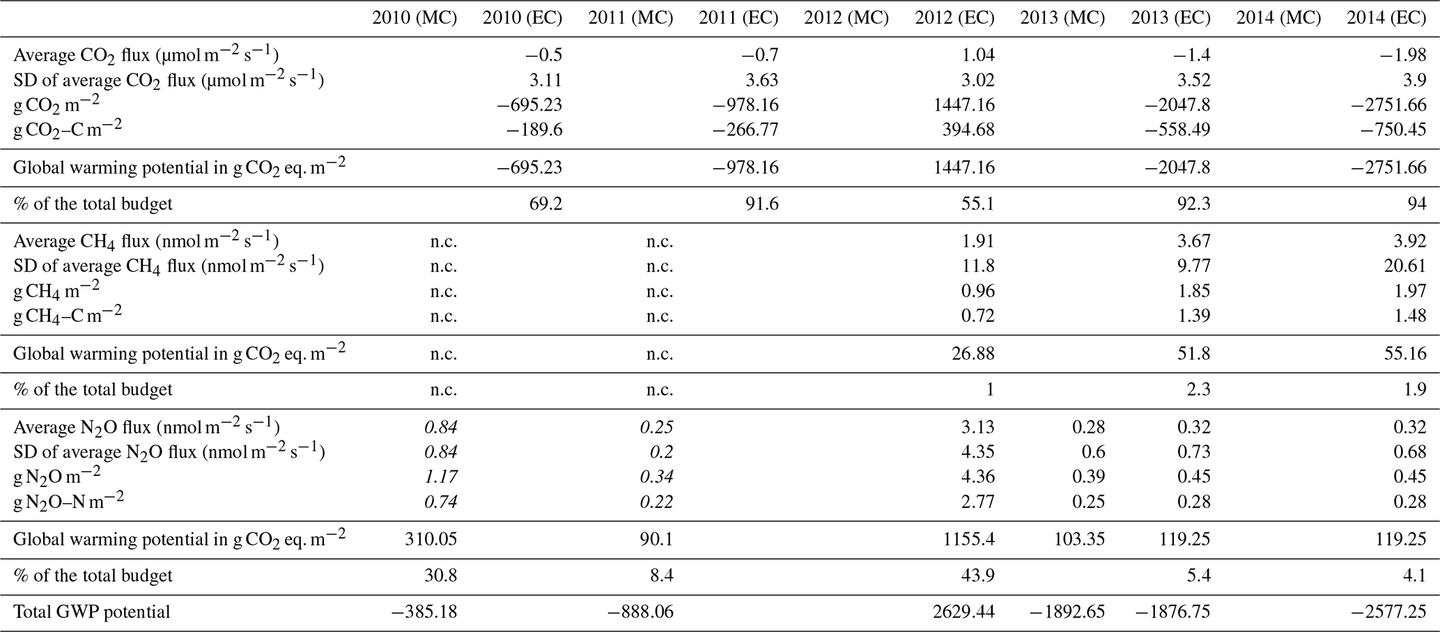
Table 2Annual average CO2, CH4 and N2O fluxes and annual sums for the three GHGs as well as carbon and nitrogen gain and losses per gas species. GWP was calculated for a 100-year time horizon and based on the most recent numbers provided by the IPCC (Stocker et al., 2013). Annual budgets were derived from either gap-filled manual chamber (MC) or eddy covariance (EC) measurements. The term n.c. stands for not calculated. Numbers in italics for N2O in the years 2010 and 2011 are likely incomplete due to limited data availability. Sign convention: positive values denote export or release and negative values import or uptake.
3.3.2 CH4 exchange
The individual static chamber measurements (2011 and 2011) were often below the detection limit and fluctuated around zero similarly to the eddy covariance measurements (Fig. 4b). Any methane peaks expected due to freezing and thawing in late winter and early spring were not observed. Also, commonly reported net emissions of methane during grazing of animals were not seen (Fig. 4b). Seasonal differences in methane exchange did not show a clear pattern (Table 3). A comparison of methane fluxes obtained by both static GHG chambers and EC measurements as made for N2O (see next paragraph) could not be performed due to a malfunction of the respective detector in the gas chromatograph.
3.3.3 N2O exchange
N2O exchange was low during the majority of the days over the 5-year observation period, fluctuating around zero (Fig. 4c). However, clear peaks in N2O emissions were observed following fertilization events or periods with high rainfall after a dry period in summer (i.e., summer 2013 and 2014, Figs. 3a and 4c). While event-driven N2O emissions were commonly on the order of 4 to 8 nmol N2O m−2 s−1 (Fig. 4c), N2O emissions following plowing and subsequent re-sowing of the grassland in 2012 lead to up to 3 times as high N2O emissions (Fig. 4c, year 2012; see also Merbold et al., 2014). Similarly to methane, enhanced N2O emissions in late winter or early spring as reported by other studies could not be identified (Fig. 4c).
Background N2O fluxes were estimated by analyzing all high-temporal-resolution flux data but excluding the restoration year 2012 and all values 1 week after a management event. Daily average background fluxes were 0.21 ± 0.55 nmol m−2 s−1 (SE = 0.02). Differences in N2O exchange over the course of individual years became obvious when splitting the dataset into the four seasons (winter – DJF, spring – MAM, summer – JJA and fall – SON). In contrast to CO2 exchange that showed large net uptake rates in spring, N2O emissions were largest during summer (JJA) and lowest in winter (DJF). As highlighted for the other gases, the year of grassland restoration showed a completely different picture (Table 3).
3.4 Annual sums and global warming potential (GWP) of CO2, CH4 and N2O
Annual sums showed a net uptake of CO2 during the 2 pre-plowing years (−695 g CO2 and −978 g CO2 m−2 yr−1 in 2010 and 2011, respectively). Up to 3 times this net uptake was reached in 2013 and 2014, the 2 post-plowing years (−2046 g CO2 and −2751 g CO2 m−2 yr−1, Table 2). In contrast, the plowing year 2011 was characterized by a net release of CO2 (1447 g CO2 m−2 yr−1).
Methane budgets for the years 2010 and 2011 were not calculated as many of the available measurements were below the limit of detection. For the years 2012–2014, the annual methane budget showed a minor release of 26.8–55.2 g CH4 m−2 yr−1.
Table 3Average GHG flux rates per season: winter (DJF), spring (MAM), summer (JJA) and fall (SON). Values are based on gap-filled data to avoid bias from missing nighttime data (predominantly relevant for CO2). Data are only presented when continuous measurements (eddy covariance data) were available. Sign convention: positive values denote export or release and negative values import or uptake.
The Chamau site was characterized by a net release of nitrous oxide over the 5-year study period. While annual average N2O emissions ranged between 0.34 and 1.17 g N2O m−2 yr−1 in the non-plowing years, the site emitted 4.36 g N2O m−2 yr−1 in 2012. As an important note, due to the limited data availability for the years 2010 and 2011, the budgets of those years are likely incomplete.
The global warming potential (GWP), expressed as the yearly cumulative sum of all gases after their conversion to CO2 equivalents, was negative during all years (between −387 and −2577 CO2 eq. m−2) except for the plowing year 2012 (+2629 CO2 eq. m−2).
Overall, CO2 exchange contributed more than 90 % to the total GHG balance in 2011, 2013 and 2014. Clearly, CH4 exchange was of minimal importance for the GHG budget (Table 2). In 2010, the contribution of CO2 to the site's GHG budget was almost 70 % and N2O contributed about 30 %. Only in 2012, the year of restoration, did CO2 and N2O exchange contribute almost equally to the site's overall GHG budget (55.1 % and 43.9 %, respectively).
3.5 Carbon gains and losses of the Chamau site between 2010 and 2014
The Chamau site assimilated on average −441 ± 260 g CO2–C m−2 yr−1 (4410 kg C ha−1 yr−1) during the “business-as-usual” years (2010 and 2011 as well as 2013 and 2014). During the restoration year the site lost 395 g CO2–C m−2 (3950 kg C ha−1) (Table 2). Carbon losses (and/or gains) from methane were <1 g CH4–C m−2 during all 5 years.
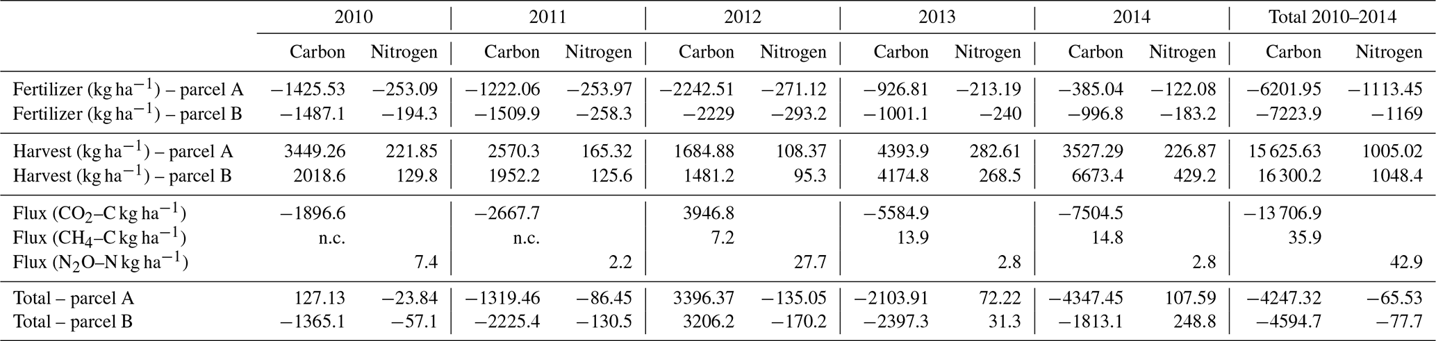
Carbon was gained in both parcels during the pre-plowing years (Table 4). Considerable net losses of carbon were calculated for the plowing year. In contrast, the post-plowing years were again recognized as years with large net gains in carbon. Over the observation period of 5 years, the Chamau grassland gained approximately 4 t C ha−1, excluding losses via leaching and deposition of C in the form of dust.
Table 4Carbon and nitrogen gains and losses through fertilization, harvest and GHGs for the Chamau (CH-Cha) site in 2010–2014. Values are given in kg ha−1. Gains are indicated with “−”, and losses or exports are indicated without “−”. While management information was available for both parcels (A and B), flux measurements represent both parcels. The term n.c. denotes not calculated.
The 5-year measurement period is representative of other similarly managed grassland ecosystems in Switzerland. Climate conditions were similar to the long-term average as described in Wolf et al. (2013). Management activities, such as harvests and subsequent fertilizer applications, were driven by overall weather conditions (i.e., 2013 late spring, Fig. 2a and b).
4.1 Technical and methodological aspects of the study
Different techniques are currently applied to measure GHG fluxes in a variety of ecosystems (Denmead, 2008), each having its advantages and disadvantages or being chosen for a specific purpose or reason. A common approach to study individual processes or time periods contributing to specific greenhouse gas emissions is to measure with GHG chambers on the plot scale (Pavelka et al., 2018). Chamber methods have been widely used to derive annual GHG and nutrient budgets (Barton et al., 2015; Butterbach-Bahl et al., 2013). Critical assessments of the suitability of and associated uncertainty in chamber-derived GHG budgets in relation to sampling frequency have been published by Barton et al. (2015). Existing studies have not only compared the two measurement techniques employed in this study (manual chambers and eddy covariance) in grasslands before but also estimated annual emissions based on differing methodologies (Flechard et al., 2007; Jones et al., 2017). Additional confidence in our approach was obtained from the N2O emissions during the summer period 2013, where both measurement techniques ran in parallel (Fig. 3a and b). Annual budgets derived by applying similar gap-filling approaches to the individual datasets led to comparable results (Table 2).
We calculated detection limits for the individual GHGs from our manual chambers following Parkin et al. (2012). Detection limits were 0.34 ± 0.26 and 0.05 ± 0.02 nmol m−2 s−1 and 0.06 ± 0.06 µmol m−2 s−1 for CH4, N2O and CO2, respectively. Following this, methane flux measurements were frequently below this limit of detection; hence we did not calculate methane budgets for 2010 and 2011. The flux values measured with the EC technique between 2012 and 2014 compare well to similar measurements made by Felber et al. (2016) in an intensively managed grassland in western Switzerland. The observed values have been identified to represent the soil methane exchange in EC measured fluxes (Felber et al., 2016).
N2O fluxes in contrast were much better constrained by both methods due to clear N2O sources (i.e., fertilizer amendments) and better sensitivity of the instruments used by both techniques for N2O as compared to CH4. Background N2O emissions as observed in this study (0.21 ± 0.55 nmol m−2 s−1 (SE = 0.02)) compare well to estimates suggested by Rafique et al. (2011), who suggest an annual background N2O loss of 1.8 kg N2O–N for a grazed pasture (i.e., 0.20 nmol m−2 s−1).
4.2 Annual GHG and C and N gains and losses
Net carbon losses and gains estimated for the CH-Cha site between 2010 and 2015 were in general within the range of values estimated by Zeeman et al. (2010) for the years 2006 and 2007. The slightly higher losses observed prior to plowing may result from reduced productivity of the sward. This becomes particularly visible when compared to the net ecosystem exchange (NEE) of CO2 values for the years after restoration. Losses via leaching have previously been estimated to be of minor importance at this site (Zeeman et al., 2010) and were therefore not considered in this study. Considerably higher C gains during post-plowing years were caused be enhanced plant growth in spring and summer. Restoration is primarily performed to eradicate weeds and rodents, favoring biomass productivity of the fodder grass composition. Other grasslands in central Europe, i.e., sites in Austria, France and Germany, showed similar values for net ecosystem exchange (Hörtnagl et al., 2018). Still, total C budgets as presented here are subject to considerable uncertainty which is strongly dependent on assumptions made for, e.g., gap filling (Foken et al., 2004). Nevertheless, the values reported here show the overall trend in C uptake and release of the site and clearly exceed the uncertainty of ± 50 g C per year for eddy covariance studies as suggested by Baldocchi (2003).
Table 5Existing studies investigating the GHG exchange over pastures following plowing. Results presented show the flux magnitude following plowing and are rounded values of the individual values presented in the papers. Values were converted to similar units (mg CO2–C, µg CH4–C and µg N2O–N m−2 h−1). This is based on a Web of Knowledge (now called Web of Science) search on 15 July 2017 with the search terms “grassland”, “pasture”, “greenhouse gas”, “plowing” and/or “tillage”. Only two studies representing conversion from pasture to cropland or other systems are included in this table.
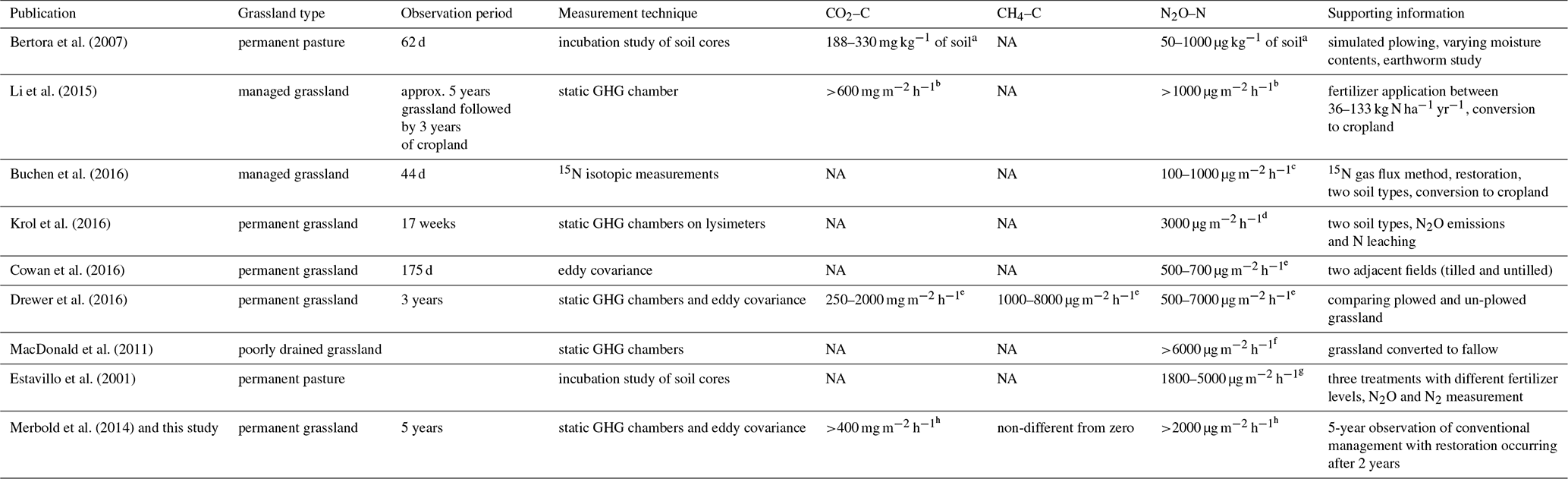
a Cumulative fluxes over 62 d. b Conversion from grassland to cropland. c Approximate value recalculated from figure in the paper. d Approximate peak emission following restoration calculated from figure in the paper. e Approximate value recalculated from figures presented in both papers. f Approximate value recalculated from figure in the paper. g Approximate value presented in Fig. 3 in the publication. h Peak emissions following plowing. NA: not available.
Methane was of negligible importance for the C budget of this site. We did not observe distinct peaks in CH4 emissions in relation to grazing which is primarily due to the low grazing pressure at CH-Cha. Studies carried out on pastures in Scotland, Mongolia, France and western Switzerland have shown that grazing can largely contribute to ecosystem-scale methane fluxes, in particular if ruminants such as cattle populate the EC footprint (Dengel et al., 2011; Felber et al., 2015; Schönbach et al., 2012). If we included an approximation of methane emissions of cattle which we may have missed in the EC flux measurements, we would have to add 3.67 g CH4–C m−2 yr−1 to the current value of 1.48 g CH4–C m−2 in 2014 (Table 2). This value is based on the average methane emissions of 404 g CH4 per head per day stated in Felber et al. (2016) and linked to the average stocking density (4.04 head ha−1) on the Chamau site and the stocking duration (30 d in 2014). Still, the GHG budget as well as the C budget of the site would not be altered.
The nitrous oxide budget reported for the years without plowing in this study coincides with values reported for other grasslands in Europe (Table 5), ranging from moist to dry climates and lower to higher elevations in Austria and Switzerland (Cowan et al., 2016; Hörtnagl et al., 2018; Imer et al., 2013; Skiba et al., 2013).
Nitrogen inputs and losses via N2O varied largely between the years before and after plowing. While the site was characterized by large N amendments prior to plowing and with reduced harvest, the picture was completely the opposite during the years after plowing, with considerably fewer N inputs compared to the nitrogen removed from the field via harvests. Farmers aim at having a balanced N budget every year (fertilizer inputs equal to nutrients removed from the field). Pasture degradation is the main motivation for enhanced fertilizer inputs in order to stabilize forage productivity. Similarly, regular restoration of permanent pastures is absolutely necessary (Cowan et al., 2016). So far, we have identified only one study that investigated the net effects on the overall GHG exchange following grassland restoration (Drewer et al., 2017).
This study in combination with an overview of available datasets on grassland restoration and their consequences for GHG budgets highlights the overall need for additional observational data. While restoration changed the previous C sink to a C source at the Chamau site, the wider implication in terms of the GWP of the site when including other GHGs have long-term consequences (i.e., in mitigation assessments). Furthermore, this study showed the large variations in N inputs and N outputs from this grassland and the difficulty farmers face when aiming for balanced N budgets in the field. Still, the current study focused on GHGs only and can thus not constrain the N budget but assess the losses of N via N2O. Losses in the form of NH3, N2 and NOx will have to be quantified to fully assess N budgets besides the overall fact that GHG data following grassland restoration remain largely limited for investigating long-term consequences. Fortunately, these are likely to become available in the near future by the establishment of environmental research infrastructures (i.e., ICOS in Europe, NEON in the USA or TERN in Australia) that aim at achieving standardized, high-quality and high-temporal-resolution trace gas observation of major ecosystems, including permanent grasslands. With these additional data, another major constraint of producing defensible GHG and nutrient budgets, namely gap-filling procedures, will likely be overcome. New and existing data can be used to derive reliable functional relations and artificial neural networks (ANNs) at a field to ecosystem scale that are capable of reproducing data measured in situ. Once this step is achieved, both the available data and the functional relations can be used to improve, train and validate existing biogeochemical process models (Fuchs et al., 2020). Subsequently, reliable projections of both nutrient and GHG budgets at the ecosystem scale that are driven by anthropogenic management as well as climatic variability can become reality.
The study stresses the necessity of including management activities occurring at a low frequency such as plowing in GHG and nutrient budget estimates. Only then can the effect of potential best-bet climate change mitigation options be thoroughly quantified. The next steps in GHG observations from grassland must not only focus on observing business-as-usual activities but also aim at testing the just-mentioned best-bet mitigation options jointly in the field while simultaneously in combination with existing biogeochemical process models.
All flux and metadata are openly available via FLUXNET. The flux processing code is available via the Grassland Sciences Group at ETH Zurich. Greenhouse gas chamber data are available via Imer et al. (2013).
The supplement related to this article is available online at: https://doi.org/10.5194/bg-18-1481-2021-supplement.
LM and LH designed the study and wrote the first manuscript version. LM, CD, WE, KF and BW collected the data in the field. LH further provided the code for flux processing. All authors revised and commented on the manuscript.
The authors declare that they have no conflict of interest..
Funding for this study is gratefully acknowledged and was provided by the following projects: Models4Pastures (FACCE-JPI project, SNSF-funded contract 40FA40_154245/1), GHG-Europe (FP7, EU contract no. 244122), COST-ES0804 ABBA and SNF R'Equip (206021_133763). We are specifically thankful to Hans-Rudolf Wettstein, Ivo Widmer and Tina Stiefel for providing crucial management data and support in the field. Further, this project could not have been accomplished without the help from the technical team, specifically Peter Plüss, Thomas Baur, Florian Käslin, Philip Meier and Patrick Flütsch. We greatly acknowledge their help during the planning stage and their endurance during the setup of the new QCLAS system as well as their regular troubleshooting of the Swiss FluxNet Chamau (CH-Cha) research site.
This research has been supported by the Swiss National Science Foundation (SNSF; contract number 40FA40_154245) as well as by the European Union Seventh Framework Programme (FP7, 2007–2013) under grant greement no. 244122 (GHG-Europe).
This paper was edited by Sara Vicca and reviewed by two anonymous referees.
Ambus, P., Clayton, H., Arah, J. R. M., Smith, K. A., and Christensen, S.: Similar N2O flux from soil measured with different chamber techniques, Atmos. Environ. A-Gen., 27, 121–123, https://doi.org/10.1016/0960-1686(93)90078-D, 1993.
Ammann, C., Neftel, A., Jocher, M., Fuhrer, J., and Leifeld, J.: Effect of management and weather variations on the greenhouse gas budget of two grasslands during a 10-year experiment, Agr. Ecosyst. Environ., 292, 106814, https://doi.org/10.1016/j.agee.2019.106814, 2020.
Baldocchi, D.: Measuring fluxes of trace gases and energy between ecosystems and the atmosphere – the state and future of the eddy covariance method, Global Change Biol., 20, 3600–3609, https://doi.org/10.1111/gcb.12649, 2014.
Baldocchi, D., Detto, M., Sonnentag, O., Verfaillie, J., Teh, Y. A., Silver, W., and Kelly, N. M.: The challenges of measuring methane fluxes and concentrations over a peatland pasture, Agr. Forest Meteorol., 153, 177–187, https://doi.org/10.1016/j.agrformet.2011.04.013, 2012.
Baldocchi, D. D.: Assessing the eddy covariance technique for evaluating carbon dioxide exchange rates of ecosystems: Past, present and future, Global Change Biol., 9, 479–492, https://doi.org/10.1046/j.1365-2486.2003.00629.x, 2003.
Ball, B. C., Scott, A., and Parker, J. P.: Field N2O, CO2 and CH4 fluxes in relation to tillage, compaction and soil quality in Scotland, Soil Till. Res., 53, 29–39, https://doi.org/10.1016/S0167-1987(99)00074-4, 1999.
Barton, L., Wolf, B., Rowlings, D., Scheer, C., Kiese, R., Grace, P., Stefanova, K., and Butterbach-Bahl, K.: Sampling frequency affects estimates of annual nitrous oxide fluxes, Sci. Rep.-UK, 5, 15912, https://doi.org/10.1038/srep15912, 2015.
Brümmer, C., Lyshede, B., Lempio, D., Delorme, J.-P., Rüffer, J. J., Fuß, R., Moffat, A. M., Hurkuck, M., Ibrom, A., Ambus, P., Flessa, H., and Kutsch, W. L.: Gas chromatography vs. quantum cascade laser-based N2O flux measurements using a novel chamber design, Biogeosciences, 14, 1365–1381, https://doi.org/10.5194/bg-14-1365-2017, 2017.
Buchen, C., Well, R., Helfrich, M., Fuß, R., Kayser, M., Gensior, A., Benke, M., and Flessa, H.: Soil mineral N dynamics and N2O emissions following grassland renewal, Agr. Ecosyst. Environ., 246, 325–342, https://doi.org/10.1016/j.agee.2017.06.013, 2017.
Butterbach-Bahl, K., Kiese, R., and Liu, C.: Measurements of biosphere atmosphere exchange of CH4 in terrestrial ecosystems, Method. Enzymol., 495, 271–287, 2011.
Butterbach-Bahl, K., Baggs, E. M., Dannenmann, M., Kiese, R., and Zechmeister-Boltenstern, S.: Nitrous oxide emissions from soils: How well do we understand the processes and their controls?, Philos. T. Roy. Soc. B, 368, 20130122, https://doi.org/10.1098/rstb.2013.0122, 2013.
Chen, Z., Ding, W., Xu, Y., Müller, C., Yu, H., and Fan, J.: Increased N2O emissions during soil drying after waterlogging and spring thaw in a record wet year, Soil Biol. Biochem., 101, 152–164, https://doi.org/10.1016/j.soilbio.2016.07.016, 2016.
Ciais, P., Reichstein, M., Viovy, N., Granier, A., Ogée, J., Allard, V., Aubinet, M., Buchmann, N., Bernhofer, C., Carrara, A., Chevallier, F., De Noblet, N., Friend, A. D., Friedlingstein, P., Grünwald, T., Heinesch, B., Keronen, P., Knohl, A., Krinner, G., Loustau, D., Manca, G., Matteucci, G., Miglietta, F., Ourcival, J. M., Papale, D., Pilegaard, K., Rambal, S., Seufert, G., Soussana, J. F., Sanz, M. J., Schulze, E. D., Vesala, T., and Valentini, R.: Europe-wide reduction in primary productivity caused by the heat and drought in 2003, Nature, 437, 529–533, https://doi.org/10.1038/nature03972, 2005.
Cowan, N. J., Levy, P. E., Famulari, D., Anderson, M., Drewer, J., Carozzi, M., Reay, D. S., and Skiba, U. M.: The influence of tillage on N2O fluxes from an intensively managed grazed grassland in Scotland, Biogeosciences, 13, 4811–4821, https://doi.org/10.5194/bg-13-4811-2016, 2016.
Dengel, S., Levy, P. E., Grace, J., Jones, S. K., and Skiba, U. M.: Methane emissions from sheep pasture, measured with an open-path eddy covariance system, Global Change Biol., 17, 3524–3533, https://doi.org/10.1111/j.1365-2486.2011.02466.x, 2011.
Denmead, O. T.: Approaches to measuring fluxes of methane and nitrous oxide between landscapes and the atmosphere, Plant Soil, 309, 5–24, https://doi.org/10.1007/s11104-008-9599-z, 2008.
Drewer, J., Anderson, M., Levy, P. E., Scholtes, B., Helfter, C., Parker, J., Rees, R. M., and Skiba, U. M.: The impact of ploughing intensively managed temperate grasslands on N2O, CH4 and CO2 fluxes, Plant Soil, 411, 193–208, https://doi.org/10.1007/s11104-016-3023-x, 2017.
Eugster, W. and Plüss, P.: A fault-tolerant eddy covariance system for measuring CH4 fluxes, Agr. Forest Meteorol., 150, 841–851, https://doi.org/10.1016/j.agrformet.2009.12.008, 2010.
Eugster, W. and Merbold, L.: Eddy covariance for quantifying trace gas fluxes from soils, SOIL, 1, 187–205, https://doi.org/10.5194/soil-1-187-2015, 2015.
Felber, R., Münger, A., Neftel, A., and Ammann, C.: Eddy covariance methane flux measurements over a grazed pasture: effect of cows as moving point sources, Biogeosciences, 12, 3925–3940, https://doi.org/10.5194/bg-12-3925-2015, 2015.
Felber, R., Bretscher, D., Münger, A., Neftel, A., and Ammann, C.: Determination of the carbon budget of a pasture: effect of system boundaries and flux uncertainties, Biogeosciences, 13, 2959–2969, https://doi.org/10.5194/bg-13-2959-2016, 2016.
Flechard, C. R., Ambus, P., Skiba, U., Rees, R. M., Hensen, A., van Amstel, A., van den Pol-van Dasselaar, A., Soussana, J. F., Jones, M., Clifton-Brown, J., Raschi, A., Horvath, L., Neftel, A., Jocher, M., Ammann, C., Leifeld, J., Fuhrer, J., Calanca, P., Thalman, E., Pilegaard, K., Di Marco, C., Campbell, C., Nemitz, E., Hargreaves, K. J., Levy, P. E., Ball, B. C., Jones, S. K., van de Bulk, W. C. M., Groot, T., Blom, M., Domingues, R., Kasper, G., Allard, V., Ceschia, E., Cellier, P., Laville, P., Henault, C., Bizouard, F., Abdalla, M., Williams, M., Baronti, S., Berretti, F., and Grosz, B.: Effects of climate and management intensity on nitrous oxide emissions in grassland systems across Europe, Agr. Ecosyst. Environ., 121, 135–152, https://doi.org/10.1016/j.agee.2006.12.024, 2007.
Foken, T., Gockede, M., Mauder, M., Mahrt, L., Amiro, B., and Munger, W.: Post-Field Data Quality Control, in: Handbook of Micrometeorology, edited by: Lee, X., Massman, W., and Law, B., Atmospheric and Oceanographic Sciences Library, Vol. 29, Springer, Dordrecht, https://doi.org/10.1007/1-4020-2265-4_9, 2004.
Fratini, G. and Mauder, M.: Towards a consistent eddy-covariance processing: an intercomparison of EddyPro and TK3, Atmos. Meas. Tech., 7, 2273–2281, https://doi.org/10.5194/amt-7-2273-2014, 2014.
Fratini, G., McDermitt, D. K., and Papale, D.: Eddy-covariance flux errors due to biases in gas concentration measurements: origins, quantification and correction, Biogeosciences, 11, 1037–1051, https://doi.org/10.5194/bg-11-1037-2014, 2014.
Fuchs, K., Hörtnagl, L., Buchmann, N., Eugster, W., Snow, V., and Merbold, L.: Management matters: testing a mitigation strategy for nitrous oxide emissions using legumes on intensively managed grassland, Biogeosciences, 15, 5519–5543, https://doi.org/10.5194/bg-15-5519-2018, 2018.
Fuchs, K., Merbold, L., Buchmann, N., Bretscher, D., Brilli, L., Fitton, N., Topp, C. F. E., Klumpp, K., Lieffering, M., Martin, R., Newton, P. C. D., Rees, R. M., Rolinski, S., Smith, P. and Snow, V.: Multimodel Evaluation of Nitrous Oxide Emissions From an Intensively Managed Grassland, J. Geophys. Res.-Biogeo., 125, e2019JG005261, https://doi.org/10.1029/2019JG005261, 2020.
Hartmann, A. A. and Niklaus, P. A.: Effects of simulated drought and nitrogen fertilizer on plant productivity and nitrous oxide (N2O) emissions of two pastures, Plant Soil, 361, 411–426, https://doi.org/10.1007/s11104-012-1248-x, 2012.
Hopkins, A. and Del Prado, A.: Implications of climate change for grassland in Europe: Impacts, adaptations and mitigation options: A review, Grass Forage Sci., 62, 118–126, https://doi.org/10.1111/j.1365-2494.2007.00575.x, 2007.
Hörtnagl, L. and Wohlfahrt, G.: Methane and nitrous oxide exchange over a managed hay meadow, Biogeosciences, 11, 7219–7236, https://doi.org/10.5194/bg-11-7219-2014, 2014.
Hörtnagl, L., Barthel, M., Buchmann, N., Eugster, W., Butterbach-Bahl, K., Díaz-Pinés, E., Zeeman, M., Klumpp, K., Kiese, R., Bahn, M., Hammerle, A., Lu, H., Ladreiter-Knauss, T., Burri, S., and Merbold, L.: Greenhouse gas fluxes over managed grasslands in Central Europe, Global Change Biol., 24, 1843–1872, https://doi.org/10.1111/gcb.14079, 2018.
Imer, D., Merbold, L., Eugster, W., and Buchmann, N.: Temporal and spatial variations of soil CO2, CH4 and N2O fluxes at three differently managed grasslands, Biogeosciences, 10, 5931–5945, https://doi.org/10.5194/bg-10-5931-2013, 2013.
IPCC: Climate Change 2013: The Physical Science Basis, Contribution of Working Group I to the Fifth Assessment Report of the Intergovern-mental Panel on Climate Change, edited by: Stocker, T. F., Qin, D., Plattner, G.-K., Tignor, M., Allen, S. K., Boschung, J., Nauels, A., Xia, Y., Bex, V., and Midgley, P. M., Cambridge University Press, Cambridge, United Kingdom and New York, NY, USA, 1535 pp., 2013.
Jones, S. K., Helfter, C., Anderson, M., Coyle, M., Campbell, C., Famulari, D., Di Marco, C., van Dijk, N., Tang, Y. S., Topp, C. F. E., Kiese, R., Kindler, R., Siemens, J., Schrumpf, M., Kaiser, K., Nemitz, E., Levy, P. E., Rees, R. M., Sutton, M. A., and Skiba, U. M.: The nitrogen, carbon and greenhouse gas budget of a grazed, cut and fertilised temperate grassland, Biogeosciences, 14, 2069–2088, https://doi.org/10.5194/bg-14-2069-2017, 2017.
Knox, S. H., Sturtevant, C., Matthes, J. H., Koteen, L., Verfaillie, J., and Baldocchi, D.: Agricultural peatland restoration: Effects of land-use change on greenhouse gas (CO2 and CH4) fluxes in the Sacramento-San Joaquin Delta, Global Change Biol., 21, 750–765, https://doi.org/10.1111/gcb.12745, 2015.
Krol, D. J., Jones, M. B., Williams, M., Richards, K. G., Bourdin, F., and Lanigan, G. J.: The effect of renovation of long-term temperate grassland on N2O emissions and N leaching from contrasting soils, Sci. Total Environ., 1, 233–240, https://doi.org/10.1016/j.scitotenv.2016.04.052, 2016.
Kroon, P. S., Hensen, A., Jonker, H. J. J., Zahniser, M. S., van't Veen, W. H., and Vermeulen, A. T.: Suitability of quantum cascade laser spectroscopy for CH4 and N2O eddy covariance flux measurements, Biogeosciences, 4, 715–728, https://doi.org/10.5194/bg-4-715-2007, 2007.
Kroon, P. S., Vesala, T., and Grace, J.: Flux measurements of CH4 and N2O exchanges, Agr. Forest Meteorol., 150, 745–747, https://doi.org/10.1016/j.agrformet.2009.11.017, 2010.
Lal, R.: Soil carbon sequestration impacts on global climate change and food security, Science, 304, 1623–1627, https://doi.org/10.1126/science.1097396, 2004.
Laubach, J., Barthel, M., Fraser, A., Hunt, J. E., and Griffith, D. W. T.: Combining two complementary micrometeorological methods to measure CH4 and N2O fluxes over pasture, Biogeosciences, 13, 1309–1327, https://doi.org/10.5194/bg-13-1309-2016, 2016.
Lundegardh, H.: Carbon dioxide evolution of soil and crop growth, Soil Sci., 23, 417–453, https://doi.org/10.1097/00010694-192706000-00001, 1927.
MacDonald, J. D., Rochette, P., Chantigny, M. H., Angers, D. A., Royer, I., and Gasser, M. O.: Ploughing a poorly drained grassland reduced N2O emissions compared to chemical fallow, Soil Till. Res., 111, 123–132, https://doi.org/10.1016/j.still.2010.09.005, 2011.
MacKenzie, A. F., Fan, M. X., and Cadrin, F.: Nitrous oxide emission as affected by tillage, corn-soybean-alfalfa rotations and nitrogen fertilization, Can. J. Soil. Sci., 77, 145–152, 1997.
Matzner, E. and Borken, W.: Do freeze-thaw events enhance C and N losses from soils of different ecosystems? A review, Eur. J. Soil Sci., 59, 274–284, https://doi.org/10.1111/j.1365-2389.2007.00992.x, 2008.
Merbold, L., Eugster, W., Stieger, J., Zahniser, M., Nelson, D., and Buchmann, N.: Greenhouse gas budget (CO2, CH4 and N2O) of intensively managed grassland following restoration, Global Change Biol., 20, 1913–1928, https://doi.org/10.1111/gcb.12518, 2014.
Mishurov, M. and Kiely, G.: Gap-filling techniques for the annual sums of nitrous oxide fluxes, Agr. Forest Meteorol., 151, 1763–1767, https://doi.org/10.1016/j.agrformet.2011.07.014, 2011.
Moffat, A. M., Papale, D., Reichstein, M., Hollinger, D. Y., Richardson, A. D., Barr, A. G., Beckstein, C., Braswell, B. H., Churkina, G., Desai, A. R., Falge, E., Gove, J. H., Heimann, M., Hui, D., Jarvis, A. J., Kattge, J., Noormets, A., and Stauch, V. J.: Comprehensive comparison of gap-filling techniques for eddy covariance net carbon fluxes, Agr. Forest Meteorol., 147, 209–232, https://doi.org/10.1016/j.agrformet.2007.08.011, 2007.
Mudge, P. L., Wallace, D. F., Rutledge, S., Campbell, D. I., Schipper, L. A., and Hosking, C. L.: Carbon balance of an intensively grazed temperate pasture in two climatically: Contrasting years, Agr. Ecosyst. Environ., 144, 271–280, https://doi.org/10.1016/j.agee.2011.09.003, 2011.
Necpálová, M., Casey, I., and Humphreys, J.: Effect of ploughing and reseeding of permanent grassland on soil N, N leaching and nitrous oxide emissions from a clay-loam soil, Nutr. Cycl. Agroecosys., 95, 305–317, https://doi.org/10.1007/s10705-013-9564-y, 2013.
Nemitz, E., Mammarella, I., Ibrom, A., Aurela, M., Burba, G. G., Dengel, S., Gielen, B., Grelle, A., Heinesch, B., Herbst, M., Hörtnagl, L., Klemedtsson, L., Lindroth, A., Lohila, A., McDermitt, D. K., Meier, P., Merbold, L., Nelson, D., Nicolini, G., Nilsson, M. B., Peltola, O., Rinne, J., and Zahniser, M.: Standardisation of eddy-covariance flux measurements of methane and nitrous oxide, Int. Agrophys., 32, 517–549, https://doi.org/10.1515/intag-2017-0042, 2018.
Parkin, T. B., Venterea, R. T., and Hargreaves, S. K.: Calculating the Detection Limits of Chamber-based Soil Greenhouse Gas Flux Measurements, J. Environ. Qual., 41, 705–715, https://doi.org/10.2134/jeq2011.0394, 2012.
Pavelka, M., Acosta, M., Kiese, R., Altimir, N., Brümmer, C., Crill, P., Darenova, E., Fuß, R., Gielen, B., Graf, A., Klemedtsson, L., Lohila, A., Longdoz, B., Lindroth, A., Nilsson, M., Jiménez, S. M., Merbold, L., Montagnani, L., Peichl, M., Pihlatie, M., Pumpanen, J., Ortiz, P. S., Silvennoinen, H., Skiba, U., Vestin, P., Weslien, P., Janous, D., and Kutsch, W.: Standardisation of chamber technique for CO2, N2O and CH4 fluxes measurements from terrestrial ecosystems, Int. Agrophys., 32, 569–587, https://doi.org/10.1515/intag-2017-0045, 2018.
Pumpanen, J., Kolari, P., Ilvesniemi, H., Minkkinen, K., Vesala, T., Niinistö, S., Lohila, A., Larmola, T., Morero, M., Pihlatie, M., Janssens, I., Yuste, J. C., Grünzweig, J. M., Reth, S., Subke, J. A., Savage, K., Kutsch, W., Østreng, G., Ziegler, W., Anthoni, P., Lindroth, A., and Hari, P.: Comparison of different chamber techniques for measuring soil CO2 efflux, Agr. Forest Meteorol., 123, 159–176, https://doi.org/10.1016/j.agrformet.2003.12.001, 2004.
R Core Team: R: A language and environment for statistical computing. R Foundation for Statistical Computing, Vienna, Austria, available at: http://www.R-project.org/ (last access: 28 February 2021), 2013.
Rafique, R., Hennessy, D., and Kiely, G.: Nitrous Oxide Emission from Grazed Grassland Under Different Management Systems, in: Ecosystems, Springer, 14, 563–582, https://doi.org/10.1007/s10021-011-9434-x, 2011.
Reichstein, M., Falge, E., Baldocchi, D., Papale, D., Aubinet, M., Berbigier, P., Bernhofer, C., Buchmann, N., Gilmanov, T., Granier, A., Grünwald, T., Havránková, K., Ilvesniemi, H., Janous, D., Knohl, A., Laurila, T., Lohila, A., Loustau, D., Matteucci, G., Meyers, T., Miglietta, F., Ourcival, J. M., Pumpanen, J., Rambal, S., Rotenberg, E., Sanz, M., Tenhunen, J., Seufert, G., Vaccari, F., Vesala, T., Yakir, D., and Valentini, R.: On the separation of net ecosystem exchange into assimilation and ecosystem respiration: Review and improved algorithm, Global Change Biol., 11, 1424–1439, https://doi.org/10.1111/j.1365-2486.2005.001002.x, 2005.
Rochette, P., Ellert, B., Gregorich, E. G., Desjardins, R. L., Pattey, E., Lessard, R., and Johnson, B. G.: Description of a dynamic closed chamber for measuring soil respiration and its comparison with other techniques, Can. J. Soil. Sci., 77, 195–203, https://doi.org/10.4141/S96-110, 1997.
Rutledge, S., Wall, A. M., Mudge, P. L., Troughton, B., Campbell, D. I., Pronger, J., Joshi, C., and Schipper, L. A.: The carbon balance of temperate grasslands part II: The impact of pasture renewal via direct drilling, Agr. Ecosyst. Environ., 239, 132–142, https://doi.org/10.1016/j.agee.2017.01.013, 2017.
Schönbach, P., Wolf, B., Dickhöfer, U., Wiesmeier, M., Chen, W., Wan, H., Gierus, M., Butterbach-Bahl, K., Kögel-Knabner, I., Susenbeth, A., Zheng, X., and Taube, F.: Grazing effects on the greenhouse gas balance of a temperate steppe ecosystem, Nutr. Cycl. Agroecosys., 93, 357–371, https://doi.org/10.1007/s10705-012-9521-1, 2012.
Schulze, E. D., Luyssaert, S., Ciais, P., Freibauer, A., Janssens, I. A., Soussana, J. F., Smith, P., Grace, J., Levin, I., Thiruchittampalam, B., Heimann, M., Dolman, A. J., Valentini, R., Bousquet, P., Peylin, P., Peters, W., Rödenbeck, C., Etiope, G., Vuichard, N., Wattenbach, M., Nabuurs, G. J., Poussi, Z., Nieschulze, J., and Gash, J. H.: Importance of methane and nitrous oxide for Europe's terrestrial greenhouse-gas balance, Nat. Geosci., 2, 842–850, https://doi.org/10.1038/ngeo686, 2009.
Skiba, U., Hargreaves, K. J., Beverland, I. J., O'Neill, D. H., Fowler, D., and Moncrieff, J. B.: Measurement of field scale N2O emission fluxes from a wheat crop using micrometeorological techniques, Plant Soil, 18, 139–144, https://doi.org/10.1007/BF00011300, 1996.
Skiba, U., Jones, S. K., Drewer, J., Helfter, C., Anderson, M., Dinsmore, K., McKenzie, R., Nemitz, E., and Sutton, M. A.: Comparison of soil greenhouse gas fluxes from extensive and intensive grazing in a temperate maritime climate, Biogeosciences, 10, 1231–1241, https://doi.org/10.5194/bg-10-1231-2013, 2013.
Smith, P., Martino, D., Cai, Z., Gwary, D., Janzen, H., Kumar, P., McCarl, B., Ogle, S., O'Mara, F., Rice, C., Scholes, B., Sirotenko, O., Howden, M., McAllister, T., Pan, G., Romanenkov, V., Schneider, U., Towprayoon, S., Wattenbach, M., and Smith, J.: Greenhouse gas mitigation in agriculture, Philos. T. Roy. Soc. B, 363, 789–813, https://doi.org/10.1098/rstb.2007.2184, 2008.
Teh, Y. A., Silver, W. L., Sonnentag, O., Detto, M., Kelly, M., and Baldocchi, D. D.: Large Greenhouse Gas Emissions from a Temperate Peatland Pasture, Ecosystems, 14, 311–325, https://doi.org/10.1007/s10021-011-9411-4, 2011.
Vellinga, T. V., van den Pol-van Dasselaar, A., and Kuikman, P. J.: The impact of grassland ploughing on CO2 and N2O emissions in the Netherlands, Nutr. Cycl. Agroecosys., 70, 33–45, https://doi.org/10.1023/b:fres.0000045981.56547.db, 2004.
Vickers, D. and Mahrt, L.: Quality control and flux sampling problems for tower and aircraft data, J. Atmos. Ocean. Tech., 14, 512–526, https://doi.org/10.1175/1520-0426, 1997.
Webb, E. K., Pearman, G. I., and Leuning, R.: Correction of flux measurements for density effects due to heat and water vapour transfer, Q. J. Roy. Meteor. Soc., 106, 85–100, https://doi.org/10.1002/qj.49710644707, 1980.
Wecking, A. R., Wall, A. M., Liáng, L. L., Lindsey, S. B., Luo, J., Campbell, D. I., and Schipper, L. A.: Reconciling annual nitrous oxide emissions of an intensively grazed dairy pasture determined by eddy covariance and emission factors, Agr. Ecosyst. Environ., 287, 106646, https://doi.org/10.1016/j.agee.2019.106646, 2020.
Wolf, S., Eugster, W., Ammann, C., Häni, M., Zielis, S., Hiller, R., Stieger, J., Imer, D., Merbold, L., and Buchmann, N.: Contrasting response of grassland versus forest carbon and water fluxes to spring drought in Switzerland, Environ. Res. Lett., 9, 089501, https://doi.org/10.1088/1748-9326/8/3/035007, 2013.
Zeeman, M. J., Hiller, R., Gilgen, A. K., Michna, P., Plüss, P., Buchmann, N., and Eugster, W.: Management and climate impacts on net CO2 fluxes and carbon budgets of three grasslands along an elevational gradient in Switzerland, Agr. Forest Meteorol., 150, 519–530, https://doi.org/10.1016/j.agrformet.2010.01.011, 2010.
Zenone, T., Zona, D., Gelfand, I., Gielen, B., Camino-Serrano, M., and Ceulemans, R.: CO2 uptake is offset by CH4 and N2O emissions in a poplar short-rotation coppice, GCB. Bioenergy, 8, 524–538, https://doi.org/10.1111/gcbb.12269, 2016.
Zona, D., Janssens, I. A., Gioli, B., Jungkunst, H. F., Serrano, M. C., and Ceulemans, R.: N2O fluxes of a bio-energy poplar plantation during a two years rotation period, GCB. Bioenergy, 5, 536–547, https://doi.org/10.1111/gcbb.12019, 2013.