the Creative Commons Attribution 4.0 License.
the Creative Commons Attribution 4.0 License.
 | 01 Apr 2021
Multi-scale assessment of a grassland productivity model
Dawn M. Browning
Grasslands provide many important ecosystem services globally, and projecting grassland productivity in the coming decades will provide valuable information to land managers. Productivity models can be well calibrated at local scales but generally have some maximum spatial scale in which they perform well. Here we evaluate a grassland productivity model to find the optimal spatial scale for parameterization and thus for subsequently applying it in future productivity projections for North America. We also evaluated the model on new vegetation types to ascertain its potential generality. We find the model most suitable when incorporating only grasslands, as opposed to also including agriculture and shrublands, and only in the Great Plains and eastern temperate forest ecoregions of North America. The model was not well suited to grasslands in North American deserts or northwest forest ecoregions. It also performed poorly in agriculture vegetation, likely due to management activities, and shrubland vegetation, likely because the model lacks representation of deep water pools. This work allows us to perform long-term projections in areas where model performance has been verified, with gaps filled in by future modeling efforts.
- Article
(2837 KB) - Full-text XML
-
Supplement
(418 KB) - BibTeX
- EndNote


Grassland systems span nearly 30 % of the global land surface (Adams et al., 1990) and play a prominent role in terrestrial carbon cycles (Parton et al., 2012). Grasslands in North America provide a large proportion of food and fiber agricultural products for the region. Annual productivity of grasslands in central and western North America is driven in large part by precipitation (Sala et al., 2012). Future changes in the amount, intensity, and timing of precipitation will be heterogeneous across North America (Easterling et al., 2017), resulting in heterogeneous changes to grassland productivity. For example, even with consistent shifts in climate, different locations can experience different changes in productivity due to local-scale responses (Zhang et al., 2011; Sala et al., 2012; Knapp et al., 2017). This highlights the need for models which can be resolved at small spatial and temporal scales, thus making long-term grassland productivity projections as informative as possible.
A promising method for this is low-dimensional models, which are process-based models with some simplified components (Choler et al., 2010, 2011). For example, a low-dimensional model might approximate transpiration as a function of potential evapotranspiration, soil available water, and live vegetation cover along with a single parameter. As opposed to a high-dimensional model with multiple functions accounting for leaf area index, stomatal conductance, rooting depth and surface area, etc. (Caylor et al., 2009; Asbjornsen et al., 2011), the low-dimensional model is advantageous since it can generalize across broad regions with relatively few inputs. Yet they are still susceptible to over-fitting to local conditions since parameters or model structure can be tied to specific locations or plant functional groups (Fisher and Koven, 2020). Thus parameterizing low-dimensional models must be done with care such that they are applicable to a broad area while maintaining an acceptable level of accuracy.
Here we evaluate a low-dimensional model with the intention of it driving productivity projections. The PhenoGrass model developed by Hufkens et al. (2016) is a pulse-response productivity model with temperature and precipitation as the primary drivers. The model is parameterized using observations from the PhenoCam network which have a small spatial resolution (footprints of <1 ha), sub-daily sampling, and sites across all major biomes. These attributes make the PhenoGrass model potentially widely applicable. We expand on the evaluation of the original study by using 84 PhenoCam sites, totalling 89 distinct time series with 463 site years of data. Using the original methods and input datasets we test the model's performance with this expanded dataset. We also evaluate the model across different combinations of North American ecoregions and vegetation types to find an optimal spatial scale in which to parameterize and apply the model. Finally, we address where the model performs poorly and how productivity projections for these areas could be implemented or improved.
2.1 PhenoGrass model
The PhenoGrass model is an ecohydrology model which has interacting state variables for soil water, plant available water, and plant fractional cover (Hufkens et al., 2016). Model inputs are daily precipitation, temperature, potential evapotranspiration (derived from the Hargreaves equation; Hargreaves and Samani, 1985), and solar radiation. The primary output is fractional vegetation cover (fCover). The original model form, derived in Choler et al. (2010, 2011), used only temperature and potential evapotranspiration and was parameterized using satellite-derived normalized difference vegetation index (NDVI) data. Hufkens et al. (2016) expanded on the original Choler model by incorporating growth and senescence restraints from temperature and solar radiation, and also included a scaling factor to convert PhenoCam Gcc (green chromatic coordinate) data to a fractional cover estimate (see equations in the Supplement). Hufkens et al. (2016) evaluated the PhenoGrass model using 14 grassland PhenoCam sites across western North America with a total of 34 site years. They found the modeled fractional cover correlated well with annual productivity at both daily and annual timescales. Despite its name the PhenoGrass model can theoretically apply to any vegetation type with a distinct growth signal in response to precipitation, as hypothesized in the original threshold-delay model (Ogle and Reynolds, 2004). Here we evaluate two additional vegetation types, shrubs and agricultural plots, to test how applicable it is beyond grasslands.
2.2 PhenoCam data
The PhenoCam network is a global network of fixed, near-surface cameras capturing true-color images of vegetation throughout the day (Richardson et al., 2018a). Using a ratio of the three RGB bands a greenness metric (green chromatic coordinate, Gcc) is calculated from each image, resulting in a daily-scale time series of canopy greenness. Gcc is a unitless metric which is highly correlated with satellite-derived NDVI (Richardson et al., 2018b) and flux-tower-derived primary productivity (Yan et al., 2019; Toomey et al., 2015). Each PhenoCam image is subset to one of several different plant vegetation types based on the field of view. These regions of interest (ROIs) serve as the basis for the Gcc calculation and subsequent post-processing (Seyednasrollah et al., 2019).
We downloaded all PhenoCam data with ROIs of the grassland (GR), shrubland (SH), and agricultural (AG) vegetation types for the years 2012 to 2018, totalling 89 distinct time series and 463 site years (Fig. 1; Table S2 in the Supplement). As input to the PhenoGrass model, we used the 3 d smoothed Gcc scaled, for each ROI, from 0–1. In the model parameterization each ROI time series is further transformed to fractional vegetation cover (fCover; see Supplement equations) using the local mean annual precipitation (MAP) combined with a scaling factor (Hufkens et al., 2016; Donohue et al., 2013).
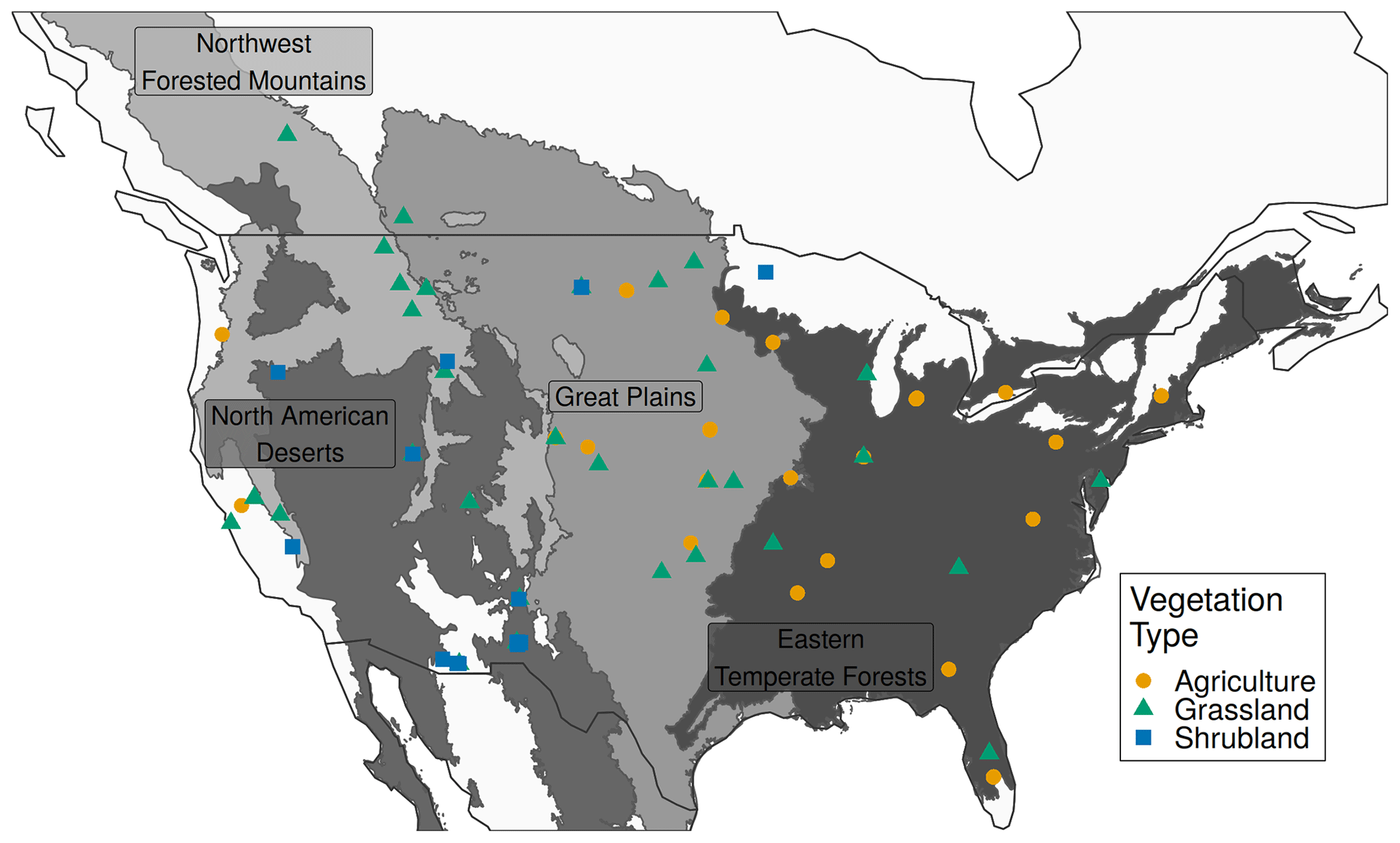
Figure 1Locations of PhenoCam sites. Color indicates the vegetation type represented at each site. Vegetation type is defined by the PhenoCam network. Shading indicates Environmental Protection Agency (EPA) North American level 1 ecoregions.
2.3 Environmental data
For historic precipitation and temperature, we used the 1 km resolution Daymet dataset (Thornton et al., 2018), extracting daily time series for the pixel at each PhenoCam tower location. Daily mean temperature was calculated as the average between the Daymet daily minimum and maximum temperatures and smoothed with a 15 d moving average. Potential evapotranspiration was calculated using the Hargreaves equation (Hargreaves and Samani, 1985). Soil wilting point and field capacity were extracted at each PhenoCam location from a global dataset (Global Soil Data Task Group, 2000). Despite other options being available we chose to use the same climate and soil datasets as those used in Hufkens et al. (2016) so that any differences in results can be attributed to the expanded PhenoCam dataset used here.
2.4 Model evaluation
To find the most appropriate spatial scale, we evaluated the model using three different combinations of ecoregion and vegetation type with 11 total model parameterizations (Fig. 2). Here we use the term “spatial scale” to refer to the combination of ecoregion(s) and vegetation type(s) used within each model. This includes using all sites of one vegetation type within an ecoregion or all sites of a specific vegetation type from several ecoregions (Fig. 2). The largest spatial scale used all PhenoCam locations described above (89 sites). Next were all sites, respectively, within the three vegetation types indicated by the ROI (grasslands, shrublands, and agricultural). Finally, we parameterized models for each vegetation type within each level 1 North American ecoregion (e.g., all grassland sites within the Great Plains ecoregion). All sets of parameterized models were limited to have at least five sites.
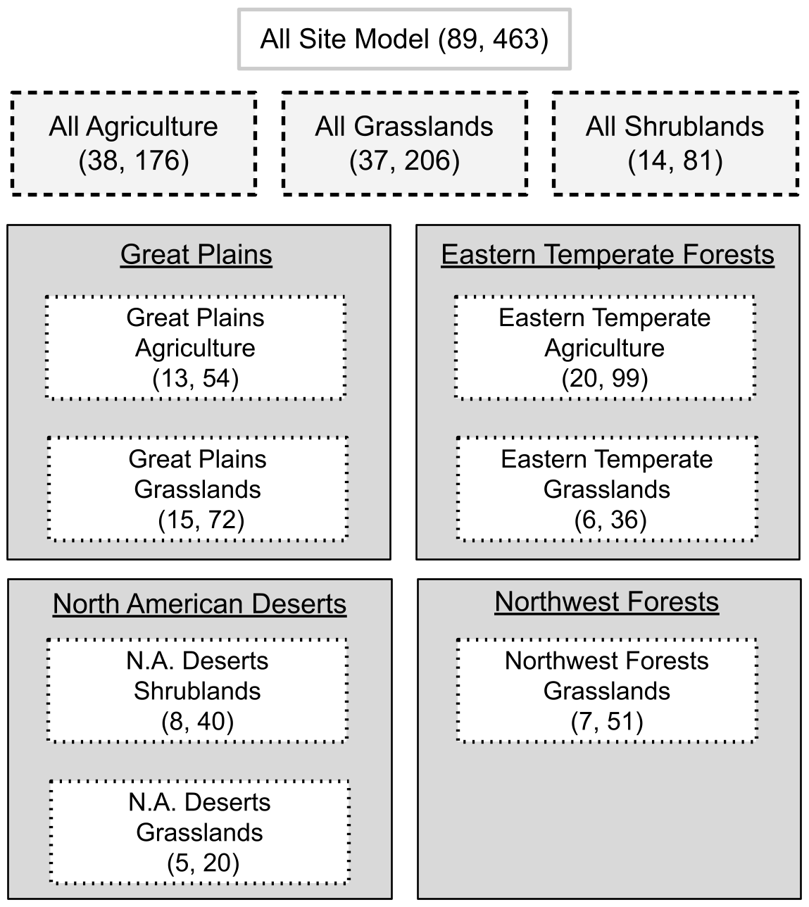
Figure 2Scaling representation of the 11 model parameterizations. Numbers in parentheses represent the number of sites and site years, respectively. Each model uses a different subset of sites ranging from the entire dataset (all site model) to one vegetation type within an ecoregion (e.g., eastern temperate forest grasslands).
We evaluated each of the 11 models using the Nash–Sutcliffe coefficient of efficiency (NSE; Eq. 2), as well as the mean coefficient of variation of the mean absolute error (F, Eq. 3) of the daily fractional cover estimates. NSE was calculated for each site and then averaged across all sites within the respective spatial scale (; Eq. 1). There was no cross-validation using out-of-sample data in the initial fitting as it would have been computationally expensive. Rather, error metrics from these in-sample tests were treated as a best case scenario of what each model parameterization can achieve. From these results we used a threshold to select which models to evaluate further using cross-validation. The threshold value was an of 0.65, which is viewed as “acceptable” for time-series models (Ritter and Muñoz-Carpena, 2013). Parameterization was done using differential evolution, a global optimization algorithm, to minimize F.
N is the number of sites within the spatial scale evaluated, n is the number of daily values at each site, fCoveri,obs and fCoveri,pred are observed and predicted values, respectively, and is the average observed fCover at each site.
Models which exceeded the threshold were subject to further evaluation. For each model we performed a leave-one-out cross-validation, in which the model was re-fit with one PhenoCam site not included in the training data and then evaluated against this left-out site. In this step a scaling coefficient to link mean annual precipitation with PhenoCam Gcc was held constant at the value obtained in the first fitting. The resulting and F are from all modeled sites using their respective out-of-sample test.
All PhenoCam data were downloaded using the PhenoCam R package (Hufkens et al., 2018). Other packages used in the R 3.6 language were dplyr (Wickham et al., 2017), tidyr (Wickham and Henry, 2018), ggplot2 (Wickham, 2016), daymetr (Hufkens et al., 2018), rgdal (Bivand et al., 2019), and sf (Pebesma, 2018). Python 3.7 packages included SciPy (Virtanen et al., 2020), NumPy (van der Walt et al., 2011), pandas (McKinney, 2010), and dask (Team, 2016). All code and data used in the analysis are available in the repository at: https://github.com/sdtaylor/PhenograssReplication (last access: 15 June 2020); the PhenoGrass model is implemented in a Python package https://github.com/sdtaylor/GrasslandModels (last access: 15 June 2020). Both are archived permanently on Zenodo (https://doi.org/10.5281/zenodo.3897319).
At the largest spatial scale in which the PhenoGrass model was parameterized using all 89 sites, the model performed poorly with an value of 0.31 (Table 1; Fig. 3). Models built using all sites of a respective vegetation type performed poorly as well, though they were slightly better than the all site model (Fig. 3). The best model performance was achieved when models were built using a single vegetation type subset for a single ecoregion. Grasslands within the Great Plains and eastern temperate forests ecoregions were the only instances where exceeded the 0.65 threshold, though grasslands within northwestern forests came close (NSE=0.64).
Table 1Average site-level Nash–Sutcliffe coefficient of efficiency () and mean coefficient of variation of the mean absolute error (F) for each model parameterization. Bold indicates when the was greater than the acceptable threshold of 0.65. Values in parentheses represent the or F in the leave-one-out cross-validation.
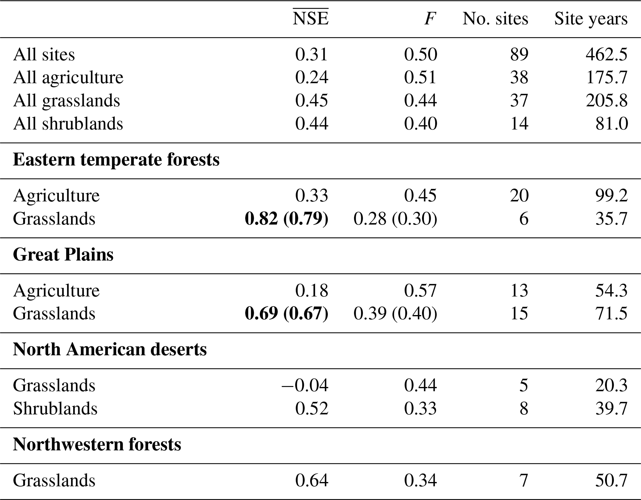
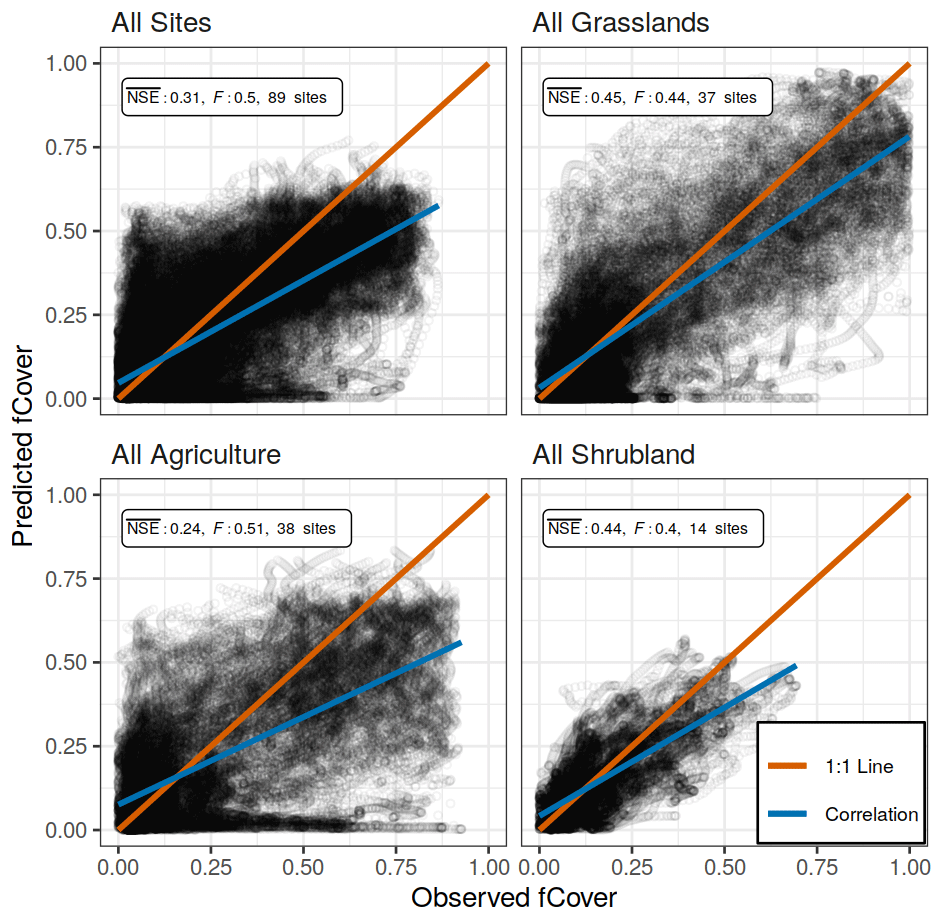
Figure 3Observed and predicted daily fCover values of the all site model and the three vegetation type models, each using all available sites and years with the respective spatial scale. NSE is the average Nash–Sutcliffe coefficient of efficiency among sites, and F is the mean coefficient of variation of the mean absolute error. The correlation line (blue) represents the overall trend in predicted versus observed values, while the 1:1 line (red) represents a perfect fit.
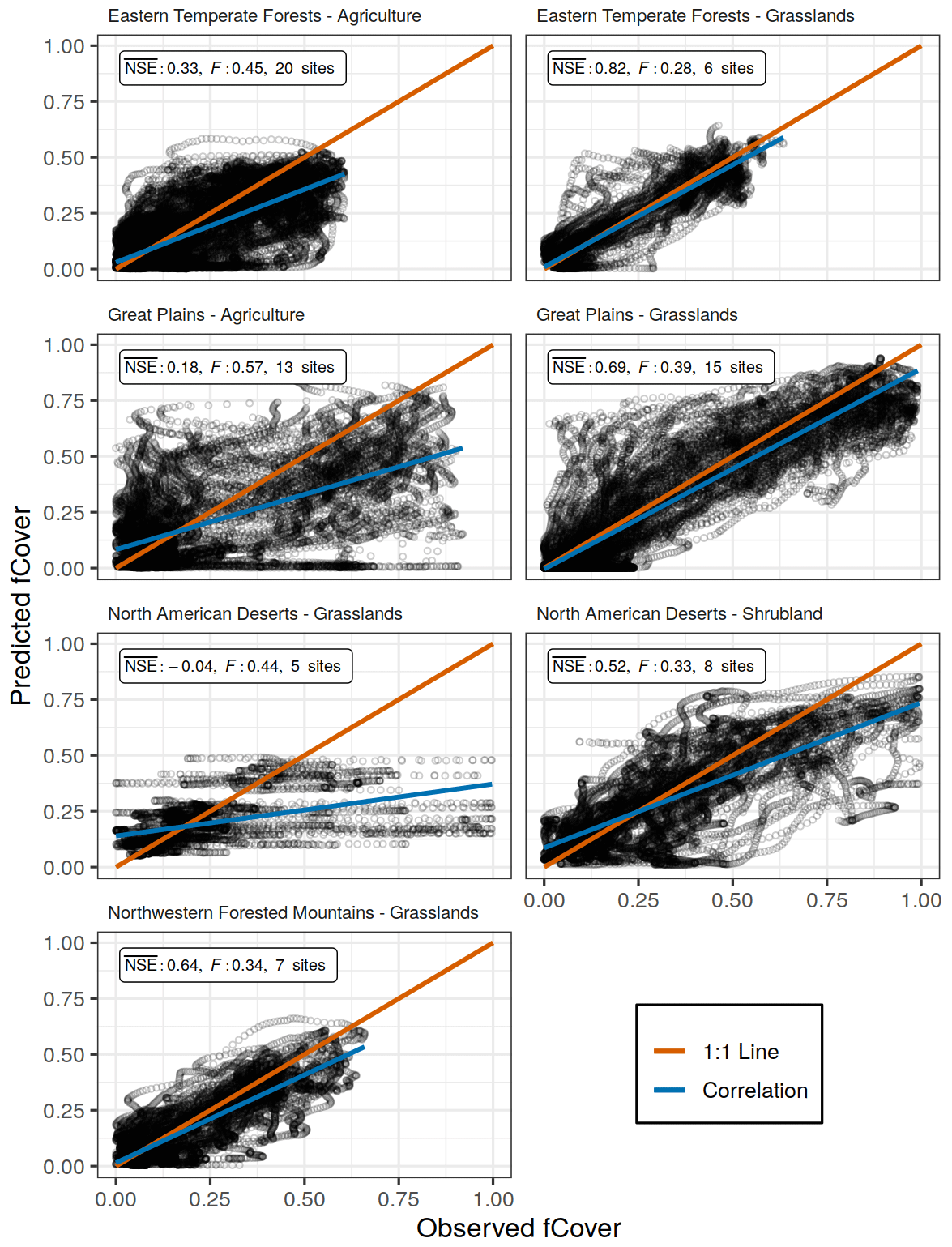
Figure 4Observed and predicted daily fCover values for models from seven spatial scales, for which only specific vegetation types within a single ecoregion were used in model fitting. Each uses all available sites and years with the respective spatial scale. NSE is the average Nash–Sutcliffe coefficient of efficiency among sites, and F is the mean coefficient of variation of the mean absolute error. The correlation line (blue) represents the overall trend in predicted versus observed values, while the 1:1 line (red) represents a perfect fit.
In all 11 models the PhenoGrass model tended to underestimate the highest fCover values and to a lesser degree overpredict the lowest values (Figs. 3 and 4). The best performing models (grasslands in the Great Plains and eastern temperate forests) minimized this effect (Fig. 4). The worst performing models, grasslands in North American deserts, had little variation in predicted fCover values, resulting in the lowest overall.
The grassland vegetation type, subset to specific ecoregions, predominantly outperformed models built with other spatial scales (Table 1). Models built using grasslands within the eastern temperate forest and Great Plains ecoregions had the highest values of 0.82 and 0.69, respectively. Using leave-one-out cross-validation on these two grassland models resulted in similar errors of 0.79 and 0.67 for the eastern temperate forest and Great Plains, respectively. Though northwestern forest grasslands had an in-sample just below the 0.65 threshold, the cross-validation was well below it (0.52). Grasslands in the North American deserts were not modeled well at any spatial scale and had the lowest values in the entire analysis. The observed greenness patterns of these desert grasslands had extremely high variability in their magnitude and timing with short distinct peaks in greenness and numerous off-peak fluctuations. The fitted model, which minimized F among the five sites, was not able to reproduce this high variability and instead produced fCover values that were severely constrained to a narrow range (Fig. S1 in the Supplement).
Agriculture and shrubland sites were poorly modeled at all spatial scales. Performance of agriculture within the eastern temperate forest ecoregion () improved over the all agriculture model () but decreased in the Great Plains ( from 0.24 to 0.18). There was only a single ecoregion with a minimum of five shrubland sites, North American deserts, and it performed only slightly better than the all shrubland model. Shrublands in North American deserts did not have the high variability seen in desert grasslands.
We performed an extensive evaluation of the PhenoGrass model across ecoregions and vegetation types to determine the best spatial scale at which to parameterize and apply the model. We found the model most suitable to grassland vegetation when constrained to the ecoregion level, though it did not perform well in grasslands in the North American desert ecoregion. Shrublands and agriculture were not well represented by the model regardless of the spatial scale. Results from this study will facilitate long-term projections of grassland productivity constrained to an appropriate vegetation type and scale.
The PhenoGrass model performed best in grassland sites embedded within ecoregions. Studies using earlier forms of the model applied it exclusively to grasslands (Choler et al., 2010, 2011; Hufkens et al., 2016), and results here confirm that it performs well in grassland vegetation with two exceptions. The model did not work in the desert grasslands, nor did it generalize well when built using all North American grasslands simultaneously. Grasslands in the North American desert biome coexist with shrubs, resulting in complex water use dynamics described in more detail below. The pulse-response design of PhenoGrass, which makes it well suited in areas with a high cover of perennial grass, is likely not applicable when grasses are interspersed with woody plants.
Shrublands were not well modeled at any spatial scale. Dryland shrubs, representing 8 of the 15 shrubland PhenoCams analyzed here, coexist with grasses by accessing different pools of soil water (Weltzin and McPherson, 2000; Muldavin et al., 2008) and thus have different responses to precipitation and resulting greenness patterns (Browning et al., 2017; Yan et al., 2019). A prior form of the PhenoGrass model was designed to work with dryland shrubs by using two soil water pools (Ogle and Reynolds, 2004), yet here PhenoGrass, with a single soil water pool, was less effective for shrubland vegetation. The single pool of the PhenoGrass model is coupled with fluxes from precipitation and evapotranspiration and thus is not well suited for representing the deeper water pools that shrubs can routinely access (Schenk and Jackson, 2002; Ward et al., 2013). Potential improvements would likely need to incorporate a deep soil water pool, in addition to the shallow pool, which are each utilized by the respective plant functional groups. This has already been implemented in highly parameterized ecohydrology models (Scanlon et al., 2005; Lauenroth et al., 2014) and could potentially be used here to make a more generalized PhenoShrub model to apply across large scales. This approach could also help in modeling North American desert grasslands which coexist among shrubs.
Agriculture areas performed poorly with the PhenoGrass model. Management practices of crops artificially increase productivity beyond what would naturally occur, and planting and harvest result in abrupt changes in greenness metrics (Bégué et al., 2018). While the results were not necessarily surprising, to our knowledge this is the first attempt to use near-surface images to drive a productivity model for agricultural vegetation. We have shown that the PhenoGrass model, designed for natural systems, does not generalize to actively managed agricultural systems. Future work in using PhenoCam data to model agricultural productivity would likely need to incorporate crop-specific parameters and management activity which other cropland modeling systems use (Fritz et al., 2019). The integration of the PhenoCam network within the Long-Term Agroecosystem Research (LTAR) network will likely be beneficial for this as the timing and intensity of management activities or experimental treatments can be incorporated into modeling efforts.
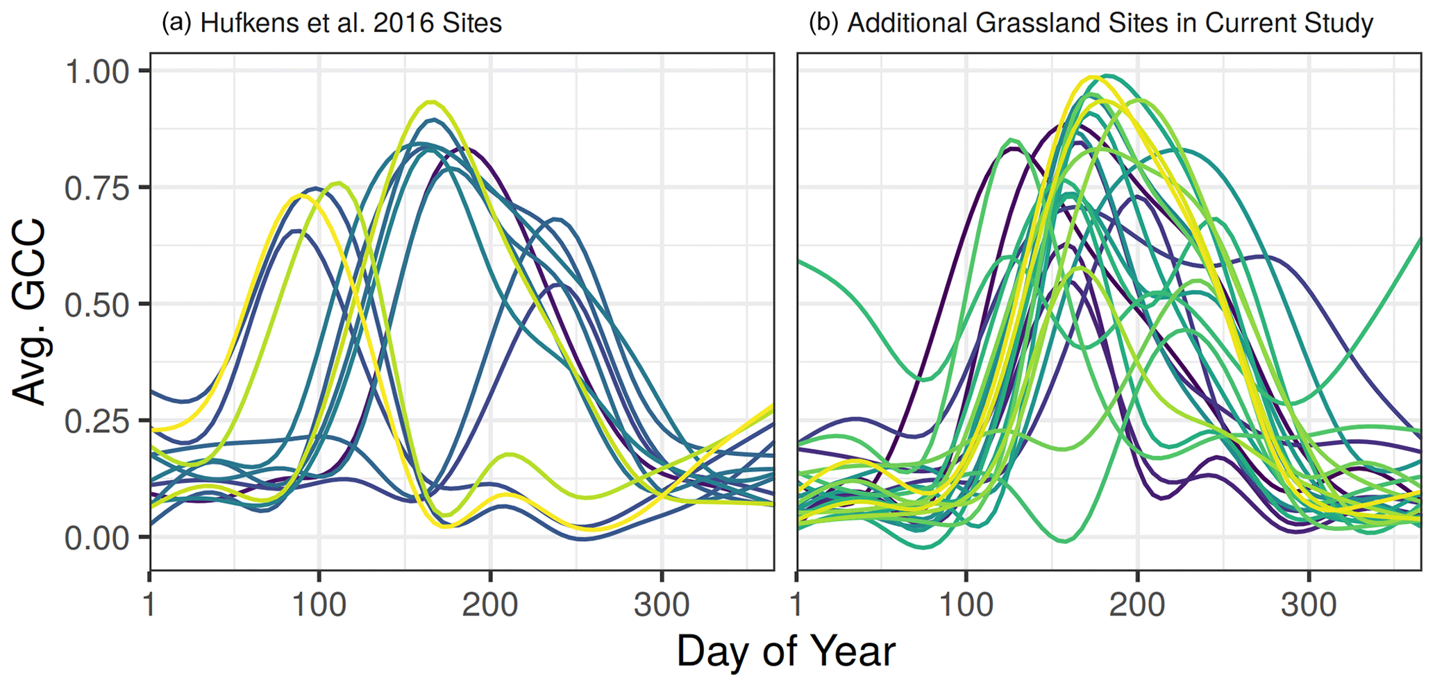
Figure 5Smoothed time series for all 14 grassland sites used in Hufkens et al. (2016) (a) and 24 additional grassland sites added in the current study (b). Each line represents the long-term average green chromatic coordinate of a single site across all available years, smoothed using a GAM model.
Hufkens et al. (2016) originally evaluated the PhenoGrass model using 14 grassland sites distributed among seven North American ecoregions. In their evaluation they had an average NSE of 0.71, while here the model performed poorly when using more than one ecoregion. It is likely that the original 14 grassland sites were ideal locations for the PhenoGrass model since on average they have a single greenup season every year in the spring or summer (Fig. 5a). The additional 24 grassland sites used in the current study have high seasonal variability and elongated growing seasons (Figs. 5b, S1) and were thus more difficult to represent in a single continental-scale grassland model. This highlights the need for longer time series in evaluating low-dimensional models as it may take many years for a single location to experience the full range of variability. As the PhenoCam data archive grows, temporally out-of-sample validation can be done to better evaluate performance in novel conditions. Further work could use the expanded PhenoCam time series to compare with flux-tower-derived productivity, which Hufkens et al. (2016) found was well correlated at the five original locations with available flux data.
Replication is an important step in the scientific process, especially given newly available data. Here we have validated prior modeling work and highlighted its limitations. Newer vegetation models can be validated in the same framework and applied to areas where PhenoGrass performs poorly. This can result in a spatial ensemble where the output for any one location and vegetation type is represented by the most appropriate model. Our current work will allow for long-term projections of grassland productivity for a large fraction of North America.
All code and data used in the analysis are available in the repository at https://github.com/sdtaylor/PhenograssReplication (last access: 15 June 2020), and the PhenoGrass model is implemented in a Python package https://github.com/sdtaylor/GrasslandModels (last access: 15 June 2020). Both are archived permanently on Zenodo (https://doi.org/10.5281/zenodo.3897319, Taylor, 2020).
The supplement related to this article is available online at: https://doi.org/10.5194/bg-18-2213-2021-supplement.
SDT designed the study and executed the modeling and analysis. SDT wrote the manuscript with input and suggestions from DMB throughout the writing process.
The authors declare that they have no conflict of interest.
This research was a contribution from the Long-Term Agroecosystem Research (LTAR) network. LTAR is supported by the United States Department of Agriculture (USDA). The authors acknowledge the USDA Agricultural Research Service (ARS) Big Data Initiative and SCINet high performance computing resources (https://scinet.usda.gov, last access: 15 June 2020) made available for conducting the research reported in this paper.
We thank our many collaborators, including site PIs and technicians, for their efforts in support of PhenoCam. The development of PhenoCam has been funded by the Northeastern States Research Cooperative, NSF's Macrosystems Biology program (awards EF-1065029 and EF-1702697), and DOE's Regional and Global Climate Modeling program (award DE-SC0016011).
This paper was edited by Ben Bond-Lamberty and reviewed by two anonymous referees.
Adams, J. M., Faure, H., Faure-Denard, L., McGlade, J. M., and Woodward, F. I.: Increases in terrestrial carbon storage from the Last Glacial Maximum to the present, Nature, 348, 711–714, https://doi.org/10.1038/348711a0, 1990. a
Asbjornsen, H., Goldsmith, G. R., Alvarado-Barrientos, M. S., Rebel, K., Van Osch, F. P., Rietkerk, M., Chen, J., Gotsch, S., Tobon, C., Geissert, D. R., Gomez-Tagle, A., Vache, K., and Dawson, T. E.: Ecohydrological advances and applications in plant-water relations research: a review, J. Plant Ecol., 4, 3–22, https://doi.org/10.1093/jpe/rtr005, https://doi.org/10.1093/jpe/rtr005, 2011. a
Bégué, A., Arvor, D., Bellon, B., Betbeder, J., de Abelleyra, D., P. D. Ferraz, R., Lebourgeois, V., Lelong, C., Simões, M., and R. Verón, S.: Remote Sensing and Cropping Practices: A Review, Remote Sens., 10, 99, https://doi.org/10.3390/rs10010099, 2018. a
Bivand, R., Keitt, T., and Rowlingson, B.: rgdal: Bindings for the “Geospatial” Data Abstraction Library, available at: https://cran.r-project.org/package=rgdal (last access: 15 June 2020), 2019. a
Browning, D. M., Maynard, J. J., Karl, J. W., and Peters, D. C.: Breaks in MODIS time series portend vegetation change: verification using long-term data in an arid grassland ecosystem, Ecol. Appl., 27, 1677–1693, https://doi.org/10.1002/eap.1561, 2017. a
Caylor, K. K., Scanlon, T. M., and Rodriguez-Iturbe, I.: Ecohydrological optimization of pattern and processes in water-limited ecosystems: A trade-off-based hypothesis, Water Resour. Res., 45, 1–15, https://doi.org/10.1029/2008WR007230, https://doi.org/10.1029/2008WR007230, 2009. a
Choler, P., Sea, W., Briggs, P., Raupach, M., and Leuning, R.: A simple ecohydrological model captures essentials of seasonal leaf dynamics in semi-arid tropical grasslands, Biogeosciences, 7, 907–920, https://doi.org/10.5194/bg-7-907-2010, 2010. a, b
Choler, P., Sea, W., and Leuning, R.: A Benchmark Test for Ecohydrological Models of Interannual Variability of NDVI in Semi-arid Tropical Grasslands, Ecosystems, 14, 183–197, https://doi.org/10.1007/s10021-010-9403-9, 2011. a, b
Donohue, R. J., Roderick, M. L., McVicar, T. R., and Farquhar, G. D.: Impact of CO2 fertilization on maximum foliage cover across the globe's warm, arid environments, Geophys. Res. Lett., 40, 3031–3035, https://doi.org/10.1002/grl.50563, 2013. a
Easterling, D. R., Kunkel, K., Arnold, J., Knutson, T. R., LeGrande, A., Leung, L., Vose, R. S., Waliser, D., and Wehner, M.: Precipitation change in the United States, in: Climate Science Special Report: Fourth National Climate Assessment, vol. I, 207–230, US Global Change Research Program, Washington, D.C., USA, https://doi.org/10.7930/J0H993CC, 2017. a
Fisher, R. A. and Koven, C. D.: Perspectives on the future of Land Surface Models and the challenges of representing complex terrestrial systems, J. Adv. Model. Earth Syst., 12, 0–3, https://doi.org/10.1029/2018ms001453, 2020. a
Fritz, S., See, L., Bayas, J. C. L., Waldner, F., Jacques, D., Becker-Reshef, I., Whitcraft, A., Baruth, B., Bonifacio, R., Crutchfield, J., Rembold, F., Rojas, O., Schucknecht, A., Van der Velde, M., Verdin, J., Wu, B., Yan, N., You, L., Gilliams, S., Mücher, S., Tetrault, R., Moorthy, I., and McCallum, I.: A comparison of global agricultural monitoring systems and current gaps, Agric. Syst., 168, 258–272, https://doi.org/10.1016/j.agsy.2018.05.010, 2019. a
Global Soil Data Task Group: Global Gridded Surfaces of Selected Soil Characteristics (IGBP-DIS), ORNL DAAC, Oak Ridge, Tennessee, USA, https://doi.org/10.3334/ORNLDAAC/569, 2000. a
Hargreaves, G. H. and Samani, Z. A.: Reference Crop Evapotranspiration from Temperature, Appl. Eng. Agric., 1, 96–99, https://doi.org/10.13031/2013.26773, 1985. a, b
Hufkens, K., Keenan, T. F., Flanagan, L. B., Scott, R. L., Bernacchi, C. J., Joo, E., Brunsell, N. A., Verfaillie, J., and Richardson, A. D.: Productivity of North American grasslands is increased under future climate scenarios despite rising aridity, Nat. Clim. Change, 6, 710–714, https://doi.org/10.1038/nclimate2942, 2016. a, b, c, d, e, f, g, h, i
Hufkens, K., Basler, D., Milliman, T., Melaas, E. K., and Richardson, A. D.: An integrated phenology modelling framework in R, Methods Ecol. Evol., 9, 1276–1285, https://doi.org/10.1111/2041-210X.12970, 2018. a, b
Knapp, A. K., Ciais, P., and Smith, M. D.: Reconciling inconsistencies in precipitation-productivity relationships: implications for climate change, New Phytol., 214, 41–47, https://doi.org/10.1111/nph.14381, 2017. a
Lauenroth, W. K., Schlaepfer, D. R., and Bradford, J. B.: Ecohydrology of Dry Regions: Storage versus Pulse Soil Water Dynamics, Ecosystems, 17, 1469–1479, https://doi.org/10.1007/s10021-014-9808-y, 2014. a
McKinney, W.: Data Structures for Statistical Computing in Python, in: Proceedings of the 9th Python in Science Conference, 51–56, SciPy, Austin, Texas, USA, https://doi.org/10.25080/Majora-92bf1922-00a, 2010. a
Muldavin, E. H., Moore, D. I., Collins, S. L., Wetherill, K. R., and Lightfoot, D. C.: Aboveground net primary production dynamics in a northern Chihuahuan Desert ecosystem, Oecologia, 155, 123–132, https://doi.org/10.1007/s00442-007-0880-2, 2008. a
Ogle, K. and Reynolds, J. F.: Plant responses to precipitation in desert ecosystems: integrating functional types, pulses, thresholds, and delays, Oecologia, 141, 282–294, https://doi.org/10.1007/s00442-004-1507-5, 2004. a, b
Parton, W., Morgan, J., Smith, D., Del Grosso, S., Prihodko, L., LeCain, D., Kelly, R., and Lutz, S.: Impact of precipitation dynamics on net ecosystem productivity, Glob. Change Biol., 18, 915–927, https://doi.org/10.1111/j.1365-2486.2011.02611.x, 2012. a
Pebesma, E.: Simple Features for R: Standardized Support for Spatial Vector Data, R J., 10, 439–446, https://doi.org/10.32614/RJ-2018-009, 2018. a
Richardson, A. D., Hufkens, K., Milliman, T., Aubrecht, D. M., Chen, M., Gray, J. M., Johnston, M. R., Keenan, T. F., Klosterman, S. T., Kosmala, M., Melaas, E. K., Friedl, M. A., and Frolking, S.: Tracking vegetation phenology across diverse North American biomes using PhenoCam imagery, Sci. Data, 5, 180 028, https://doi.org/10.1038/sdata.2018.28, 2018a. a
Richardson, A. D., Hufkens, K., Milliman, T., and Frolking, S.: Intercomparison of phenological transition dates derived from the PhenoCam Dataset V1.0 and MODIS satellite remote sensing, Sci. Rep., 8, 5679, https://doi.org/10.1038/s41598-018-23804-6, 2018b. a
Ritter, A. and Muñoz-Carpena, R.: Performance evaluation of hydrological models: Statistical significance for reducing subjectivity in goodness-of-fit assessments, J. Hydrol., 480, 33–45, https://doi.org/10.1016/j.jhydrol.2012.12.004, 2013. a
Sala, O. E., Gherardi, L. A., Reichmann, L., Jobbagy, E., and Peters, D.: Legacies of precipitation fluctuations on primary production: theory and data synthesis, Philos. T. Roy. Soc. B, 367, 3135–3144, https://doi.org/10.1098/rstb.2011.0347, 2012. a, b
Scanlon, T. M., Caylor, K. K., Manfreda, S., Levin, S. A., and Rodriguez-Iturbe, I.: Dynamic response of grass cover to rainfall variability: implications for the function and persistence of savanna ecosystems, Adv. Water Resour., 28, 291–302, https://doi.org/10.1016/j.advwatres.2004.10.014, 2005. a
Schenk, H. J. and Jackson, R. B.: Rooting depths, lateral root spreads and below-ground/above-ground allometries of plants in water-limited ecosystems, J. Ecol., 90, 480–494, https://doi.org/10.1046/j.1365-2745.2002.00682.x, 2002. a
Seyednasrollah, B., Young, A. M., Hufkens, K., Milliman, T., Friedl, M. A., Frolking, S., and Richardson, A. D.: Tracking vegetation phenology across diverse biomes using Version 2.0 of the PhenoCam Dataset, Sci. Data, 6, 222, https://doi.org/10.1038/s41597-019-0229-9, 2019. a
Taylor, S. D.: Code and data for: Multi-scale assessment of a grassland productivity model, Zenodo, https://doi.org/10.5281/zenodo.3897319, 2020. a
Team, D. D.: Dask: Library for dynamic task scheduling, available at: https://dask.org (last access: 15 June 2020), 2016. a
Thornton, P. E., Thornton, M. M., Mayer, B. W., Wei, Y., Devarakonda, R., Vose, R., and Cook, R. B.: Daymet: Daily Surface Weather Data on a 1-km Grid for North America, Version 3., Tech. rep., ORNL DAAC, Oak Ridge, Tennessee, USA, https://doi.org/10.3334/ORNLDAAC/1328, 2018. a
Toomey, M., Friedl, M. A., Frolking, S., Hufkens, K., Klosterman, S., Sonnentag, O., Baldocchi, D. D., Bernacchi, C. J., Biraud, S. C., Bohrer, G., Brzostek, E., Burns, S. P., Coursolle, C., Hollinger, D. Y., Margolis, H. A., McCaughey, H., Monson, R. K., Munger, J. W., Pallardy, S., Phillips, R. P., Torn, M. S., Wharton, S., Zeri, M., and Richardson, A. D.: Greenness indices from digital cameras predict the timing and seasonal dynamics of canopy-scale photosynthesis, Ecol. Appl., 25, 99–115, https://doi.org/10.1890/14-0005.1, 2015. a
van der Walt, S., Colbert, S. C., and Varoquaux, G.: The NumPy Array: A Structure for Efficient Numerical Computation, Comput. Sci. Eng., 13, 22–30, https://doi.org/10.1109/MCSE.2011.37, 2011. a
Virtanen, P., Gommers, R., Oliphant, T. E., Haberland, M., Reddy, T., Cournapeau, D., Burovski, E., Peterson, P., Weckesser, W., Bright, J., van der Walt, S. J., Brett, M., Wilson, J., Millman, K. J., Mayorov, N., Nelson, A. R. J., Jones, E., Kern, R., Larson, E., Carey, C. J., Polat, I., Feng, Y., Moore, E. W., VanderPlas, J., Laxalde, D., Perktold, J., Cimrman, R., Henriksen, I., Quintero, E. A., Harris, C. R., Archibald, A. M., Ribeiro, A. H., Pedregosa, F., and van Mulbregt, P.: SciPy 1.0: fundamental algorithms for scientific computing in Python, Nat. Methods, 17, 261–272, https://doi.org/10.1038/s41592-019-0686-2, 2020. a
Ward, D., Wiegand, K., and Getzin, S.: Walter's two-layer hypothesis revisited: back to the roots!, Oecologia, 172, 617–630, https://doi.org/10.1007/s00442-012-2538-y, 2013. a
Weltzin, J. F. and McPherson, G. R.: Implications of precipitation redistribution for shifts in temperate savanna ecotones, Ecology, 81, 1902–1913, 2000. a
Wickham, H.: ggplot2: Elegant Graphics for Data Analysis, Springer-Verlag, New York, available at: https://ggplot2.tidyverse.org/ (last access: 15 June 2020), 2016. a
Wickham, H. and Henry, L.: tidyr: Easily Tidy Data with 'spread()' and 'gather()' Functions, available at: https://cran.r-project.org/package=tidyr (last access: 15 June 2020), 2018. a
Wickham, H., Francois, R., Henry, L., and Müller, K.: dplyr: A Grammar of Data Manipulation, available at: https://cran.r-project.org/package=dplyr (last access: 15 June 2020), 2017. a
Yan, D., Scott, R., Moore, D., Biederman, J., and Smith, W.: Understanding the relationship between vegetation greenness and productivity across dryland ecosystems through the integration of PhenoCam, satellite, and eddy covariance data, Remote Sens. Environ., 223, 50–62, https://doi.org/10.1016/j.rse.2018.12.029, 2019. a, b
Zhang, L., Wylie, B. K., Ji, L., Gilmanov, T. G., Tieszen, L. L., and Howard, D. M.: Upscaling carbon fluxes over the Great Plains grasslands: Sinks and sources, J. Geophys. Res.-Biogeo., 116, 1–13, https://doi.org/10.1029/2010JG001504, 2011. a