Measurement and modelling of the dynamics of NH₃ surface–atmosphere exchange over the Amazonian rainforest

Local and regional modelling of NH₃ surface exchange is required to quantify nitrogen deposition to, and emissions from, the biosphere. However, measurements and model parameterisations for many remote ecosystems – such as tropical rainforest – remain sparse. Using 1 month of hourly measurements of NH₃ fluxes and meteorological parameters over a remote Amazon rainforest site (Amazon Tall Tower Observatory, ATTO), six model parameterisations based on a bidirectional, single-layer canopy compensation point resistance model were developed to simulate observations of NH₃ surface exchange. Canopy resistance was linked to either relative humidity at the canopy level (RH${}_{z_{\mathrm{0}}^{\prime }}$), vapour pressure deficit, or a parameter value based on leaf wetness measurements. The ratio of apoplastic ${\mathrm{NH}}_{\mathrm{4}}^{+}$ to H⁺ concentration, Γ_s, during this campaign was inferred to be 38.5 ± 15.8. The parameterisation that reproduced the observed net exchange of NH₃ most accurately was the model that used a cuticular resistance (R_w) parameterisation based on leaf wetness measurements and a value of Γ_s=50 (Pearson correlation r=0.71). Conversely, the model that performed the worst at replicating measured NH₃ fluxes used an R_w value modelled using RH${}_{z_{\mathrm{0}}^{\prime }}$ and the inferred value of Γ_s=38.5 (r=0.45). The results indicate that a single-layer canopy compensation point model is appropriate for simulating NH₃ fluxes from tropical rainforest during the Amazonian dry season and confirmed that a direct measurement of (a non-binary) leaf wetness parameter improves the ability to estimate R_w. Current inferential methods for determining Γ_s were noted as having difficulties in the humid conditions present at a rainforest site.

1 Introduction

The global cycling of nitrogen is of critical importance to Earth's biogeochemistry. One of the major contributors to the global atmospheric reactive nitrogen (N_r) budget is ammonia (NH₃), which is primarily generated from anthropogenic sources (Galloway et al., 2003). The emission of NH₃ and the subsequent deposition of NH₃ or other forms of reactive nitrogen have impacts on terrestrial and marine ecosystems (Erisman et al., 2013). In particular, forests can be impacted through changes to N input in several ways. Fowler et al. (2013) detail how increased deposition of N can lead to increased vegetation growth rates in forests, leading to potentially greater carbon sequestration rates. This potential positive impact, however, is offset by the effect of N saturation on forests as detailed by Nadelhoffer (2008). Here, the combined impact of disturbance to forest soil microbial systems involved in the nitrification–denitrification cycle (Fowler et al., 2009), and damage to vegetation (Krupa, 2003) leads to a sharp decrease in net primary productivity. Even at deposition rates well below the saturation values, atmospheric N_r deposition can lead to changes in plant species composition, with implication not only on biodiversity but also ecosystem services (Fowler et al., 2013). It is therefore important that exchange models be developed for all major biomes to accurately simulate NH₃ deposition rates to forests to predict potential environmental consequences.

Ammonia is emitted in small quantities from (semi-)natural sources such as wild fires and the excreta of wild animals, from plants as a result of non-zero ${\mathrm{NH}}_{\mathrm{4}}^{+}$ concentrations within the leaf apoplast, and from decomposing leaf litter; both plant sources vary with the N status of the plants. Of further importance for nitrogen modelling is therefore the determination of the extent of potential emissions from forest ecosystems and the role such NH₃ emission might play in the N_r cycle within natural forests. Forests were once considered to be perfect sinks for ammonia (Duyzer et al., 1992), until bidirectional surface exchange of NH₃ – i.e. deposition to and emission from – was recorded in many studies of NH₃ fluxes from forests (Langford and Fehsenfeld, 1992; Neirynck and Ceulemans, 2008; Wyers and Erisman, 1998). Predominantly, this has been observed in forests situated close to sources of agriculturally derived N_r pollution, although Hansen et al. (2015) also observed bidirectional fluxes over a more remote forest site.

The modelling of regional and local surface exchange of NH₃ is based on parameterisations of the exchange, which remain unverified for many biomes of global importance due to the difficulty and cost of making measurements of NH₃ fluxes. Datasets of NH₃ flux measurements have mainly been limited to temperate agricultural and semi-natural ecosystems. Consequently, very little is known about the role of NH₃ in the N cycling in remote ecosystems such as the tropics and their disturbance through anthropogenic activity. Although Flechard et al. (2015) identified the need for NH₃ surface exchange measurements over tropical ecosystems, and over rainforests in particular, such measurements have been limited so far. Here we present recent data from the Amazon Tall Tower Observatory site, situated in remote tropical rainforest, where NH₃ fluxes were measured for 1 month during the dry season of 2017 as part of a suite of species (Ramsay et al., 2020). This provides the data necessary to develop site-specific parameterisations of NH₃ surface exchange, with the potential for upscaling to the regional level. The companion paper (Ramsay et al., 2020) summarises the measured fluxes, including their statistics and average diurnal cycle, and discusses the uncertainties associated with the measurement.

As extensive reviews of NH₃ surface exchange models are available (Flechard et al., 2015; Massad et al., 2010), only a brief overview is provided here. Models of bidirectional NH₃ surface exchange consider the control of fluxes to be analogous to electrical resistances (Baldocchi, 1988; Monteith and Unsworth, 2013). Whether emission occurs from the atmosphere to the canopy or vice versa is dependent upon the relative magnitude of ambient and canopy concentrations, with resistances acting in series or in parallel impeding the exchange. In the simplest model of bidirectional surface exchange, all exchange is approximated to occur via the leaf stomata situated at a single notional mean height (big-leaf approach) and is restricted by two atmospheric resistances in series (the aerodynamic resistance and quasi-laminar boundary layer resistance), in series with a third (stomatal) resistance (stomatal compensation point model) (Sutton et al., 1993).

Increasingly complex models include further pathways of exchange (Kruit et al., 2010), with the most important for the current study being the canopy compensation point model, initially proposed by Sutton et al. (1995), which incorporates two parallel pathways of exchange at the canopy level (Fig. 1). In the first pathway, a stomatal compensation point (χ_s) is introduced, which represents the concentration of NH₃ in the leaf stomata in (temperature-dependent) equilibrium with the ${\mathrm{NH}}_{\mathrm{4}}^{+}$ and pH of the apoplastic fluid. This stomatal compensation point controls the exchange of NH₃ to and from the canopy to the leaf stomata, together with the associated stomatal resistance (R_s). In the parallel pathway, a unidirectional deposition flux is modelled from canopy to the leaf cuticle, with a separate cuticular resistance (R_w) controlling deposition. In a modified version of this model (the cuticular capacitance model), the leaf cuticle is considered to be both a sink and source for NH₃ (Sutton et al., 1998). Here, the ability of water films on the leaf cuticle surface to act as a storage of previously deposited NH₃ is introduced as an analogue of an electrical capacitor, with emission fluxes of NH₃ from the cuticle possible with the evaporation of charged water films. Further models include ones which simulate the potential for soil and leaf litter below canopy to act as emission sources of NH₃ (Nemitz et al., 2000; Sutton et al., 2009).

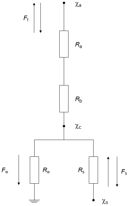
Figure 1 Schematic of the canopy compensation point model of Sutton et al. (1995). F_t, F_s, and F_w are, respectively, the total, stomatal, and cuticular fluxes of NH₃; R_a, R_b, R_w, and R_s are, respectively, the aerodynamic, quasi-laminar boundary layer, cuticular, and stomatal resistances; and χ_a, χ_c, and χ_s are, respectively, the atmospheric concentration of NH₃, the canopy compensation point, and the stomatal compensation point.

Using the static canopy compensation point model of NH₃ surface exchange, in combination with new NH₃ flux and meteorological data measured at a remote, tropical rainforest site, this study aims to present a series of local model formulations for χ_s and R_w which adequately simulate the bidirectional fluxes of NH₃ observed by Ramsay et al. (2020), with a focus on the most suitable control metric for R_w. A statistical comparison between models is conducted, with the aim to determine which parameterisation – and hence which of the factors controlling the formulation of model parameters – is best able to simulate observed fluxes. Discussion includes how meteorological conditions may have influenced model performance and how subsequent studies of NH₃ fluxes over tropical rainforest may be conducted to help improve model performance. We discuss other model frameworks, such as the dynamic CCP model, that could be used to simulate NH₃ bidirectional surface exchange in Sect. 4.1, with a focus on the simplicity and performance of the static canopy compensation point (SCCP) model as justification for not pursuing more complex models further.

2 Methodology

2.1 Field site description

Measurements were conducted on an 80 m walk-up tower located at the Amazon Tall Tower Observatory site (2^∘ 08.637^′ S, 58^∘ 59.992^′ W). The Amazon Tall Tower Observatory (ATTO) site lies on a level plateau 120 m above sea level and is situated within a region of dense, undisturbed terra firme rainforest, with a mean canopy height of 37.5 m (Chor et al., 2017). The nearest large urban centre, Manaus, Brazil, is located 150 km to the south-west. A full description of the ATTO site, its permanent instrumentation, and the floristic composition of the surrounding rainforest is given in Andreae et al. (2015).

The rainforest extends homogenously for many hundreds of kilometres to the north and east but gives way to shrub forest (campina) 5.5 km to the south, where the plateau descends to meet the Uatumã River. The flux fetch requirement for these gradient measurements with a geometric mean height of 50.2 m as determined from the approximation given by Monteith and Unsworth (2013) is 5.2 km. Therefore, NH₃ fluxes can be considered representative of a homogeneous rainforest. During convective daytime conditions, the flux footprint is much shorter, typically < 2 km.

Measurements were made between 6 October and 5 November 2017, during the region's dry season. Lasting typically from August to November, the dry season is characterised by warmer, drier conditions in comparison to the wet season, which lasts from February to May. Air masses that arrive at the site during the dry season typically travel over some urban and agricultural areas located to the south and south-east of the site, which can give rise to periods of elevated black carbon (BC) and carbon monoxide (CO) concentrations (Ramsay et al., 2020; Saturno et al., 2018).

2.2 Measurements of ammonia and meteorological parameters

2.2.1 Ammonia

Ammonia was measured using the Gradient of Aerosols and Gases Online Registration system (GRAEGOR), a semi-autonomous, continuous wet-chemistry instrument (ECN, the Netherlands) (Thomas et al., 2009). The GRAEGOR provides online analysis of a suite of inorganic trace gases (NH₃, HCl, HONO, HNO₃, and SO₂) and their associated water-soluble aerosol counterparts (${\mathrm{NH}}_{\mathrm{4}}^{+}$, Cl⁻, ${\mathrm{NO}}_{\mathrm{2}}^{-}$, ${\mathrm{NO}}_{\mathrm{3}}^{-}$, and ${\mathrm{SO}}_{\mathrm{4}}^{\mathrm{2}}-$) at two heights at hourly resolution. The instrument consists of two sample boxes, which were set at two heights (z₁=42 and z₂=60 m) on the 80 m walk-up tower, with a detector box which is connected to each sample box located in an air-conditioned container at ground level for online analysis of samples.

Each sample box contains a wet annular rotating denuder (WRD) connected in series to a steam jet aerosol collector (SJAC). A short section of high-density polyethylene (HDPE) tubing connects an inlet cone covered with an HDPE insect mesh to the sample boxes of the WRDs, ensuring that losses of NH₃ are minimised. The walls of each WRD are coated in a constantly replenishing sorption solution of 18.2 MΩ double deionised (DDI) water, with 0.6 mL of H₂O₂ (9.8 M) added per 10 L of sorption solution to eliminate potential biological contamination of the WRDs. Air is drawn simultaneously through both WRDs at a rate of 16.7 L min⁻¹, kept constant by a critical orifice downstream of the WRD. Unlike ${\mathrm{NH}}_{\mathrm{4}}^{+}$ aerosol, gaseous NH₃ diffuses through the laminar air flow onto the sorption solution coating the walls of the WRD, and the solution is subsequently transported to the detector box at ground level for analysis.

The detector box contains a flow injection analysis unit (FIA) based on a selective ion membrane to analyse the concentration of NH₃ within the WRD samples. WRD samples are fed to the FIA unit, where NaOH (0.1 M) is first added to the sample to form gaseous NH₃. The gaseous NH₃ then passes through a semi-permeable polytetrafluoroethylene (PTFE) membrane to enter a counterflow of DDI water to re-form ${\mathrm{NH}}_{\mathrm{4}}^{+}$. The temperature-corrected conductivity of ${\mathrm{NH}}_{\mathrm{4}}^{+}$ is then measured in the conductivity cell of the FIA unit, from which the atmospheric concentration of NH₃ at the height from which the sample was drawn can be determined. Through a valve control system within the detector box, the WRD sample from each height is analysed for NH₃ by FIA once per hour, resulting in an hourly-resolved concentration gradient of NH₃. The FIA unit is calibrated autonomously using three liquid ${\mathrm{NH}}_{\mathrm{4}}^{+}$ solutions (0, 50, and 500 ppb ${\mathrm{NH}}_{\mathrm{4}}^{+}$ concentration), with the first calibration conducted 24 h after the GRAEGOR begins measurements and every 72 h afterwards. Fresh standards were prepared prior to each calibration. A total of 10 autonomous calibrations were conducted during this campaign.

2.2.2 Meteorology

Wind speed (u), wind direction (wd), friction velocity (u_*), and sensible heat flux were measured by a Gill WindMaster mounted at 46 m on the 80 m walk-up tower. Relative humidity and air temperature were measured at 22, 36, and 55 m using a series of Campbell HygroVUE™ temperature and relatively humidity sensors. Net radiation and photosynthetically active radiation were measured at 75 m by, respectively, a net radiometer (Kipp and Zonnen NR-LITE2) and a quantum sensor (Kipp and Zonnen PAR LITE). Hourly rainfall was measured using a HS Hyquest TB4-L.

2.3 Modified aerodynamic gradient method

In the constant flux layer over homogeneous surfaces, the flux of a chemical tracer χ can be determined using the aerodynamic method (AGM) if the vertical concentration gradient of χ and its diffusion coefficient are known (Foken, 2008). A modified form of the AGM – based on the vertical concentration difference (Δ_c) between measurements of NH₃ at 42 and 60 m, a series of stability parameters determined from meteorological measurements, and u_* as measured at 46 m by eddy covariance (Flechard, 1998) – was used to determine the flux of NH₃ as

$$\begin{array}{}\text{(1)}& F_x=-u_{*}\mathit{\kappa }{\displaystyle \frac{{\mathrm{\Delta }}_{\mathrm{c}}}{\ln \left(\frac{z_{\mathrm{2}}-d}{z_{\mathrm{1}}-d}\right)-{\mathrm{\Psi }}_{\mathrm{H}}\left(\frac{z_{\mathrm{2}}-d}{L}\right)+{\mathrm{\Psi }}_{\mathrm{H}}\left(\frac{z_{\mathrm{1}}-d}{L}\right)}},\end{array}$$

where κ=0.41 is the von Kármán constant and d is the zero-plane displacement height, determined as 0.9 h_c=33.4 m. The integrated form of the heat stability correction term, Ψ_H, is included to account for deviations from the log-linear wind profile, while the term (z−d) $/$ L is a dimensionless measure of atmospheric stability, where L is the Obukhov length.

The aerodynamic gradient method strictly holds for measurements made within the inertial sublayer. Corrections must be applied to fluxes calculated using the AGM if measurements are made close to the canopy, within the roughness sublayer, as was the case in this study. Fluxes were corrected using a correction factor, γ_F, whose magnitude was determined from the stability conditions present at the time of measurement (Chor et al., 2017). The validity of this correction was confirmed via the flux measurements of HNO₃ and HCl by Ramsay et al. (2020).

2.4 Determination of concentrations and meteorological parameters at the aerodynamic mean canopy height

The aerodynamic resistance R_a and the quasi-laminar boundary layer R_b can be used to determine the temperature and NH₃ concentration at the aerodynamic mean canopy height, $z_{\mathrm{0}}^{\prime }$, if their respective values at a reference height are known (Nemitz et al., 2009):

$$\begin{array}{}\text{(2)}& {\displaystyle }{T}_{z_{\mathrm{0}}^{\prime }}=T(z-d){\displaystyle \frac{H}{\mathit{\rho }{c}_p}}\left(R_{\mathrm{a}}(z-d)+R_{\mathrm{b}}\right),\text{(3)}& {\displaystyle }{\mathit{\chi }}_{z_{\mathrm{0}}^{\prime }}=\mathit{\chi }(z-d)+F_{\mathit{\chi }}\left(R_{\mathrm{a}}(z-d)+R_{\mathrm{b}}\right).\end{array}$$

The relative humidity at $z_{\mathrm{0}}^{\prime }$ can be determined if the saturation pressure at $z_{\mathrm{0}}^{\prime }$ (${\mathit{\epsilon }}_{\mathrm{sat}}(T_{z_{\mathrm{0}}^{\prime }}$)) and the water vapour pressure at $z_{\mathrm{0}}^{\prime }$ (${\mathit{\epsilon }}_{z_{\mathrm{0}}^{\prime }}$) are known. ${\mathit{\epsilon }}_{z_{\mathrm{0}}^{\prime }}$ can be calculated as

$$\begin{array}{}\text{(4)}& {\mathit{\epsilon }}_{z_{\mathrm{0}}^{\prime }}=\mathit{\epsilon }(z-d)+F_{{\mathrm{H}}_{\mathrm{2}}\mathrm{O}}\left(R_{\mathrm{a}}(z-d)+R_{\mathrm{b}}\right),\end{array}$$

where $F_{{\mathrm{H}}_{\mathrm{2}}\mathrm{O}}$ is the measured water vapour flux, as taken at the 80 m tower. RH${}_{z_{\mathrm{0}}^{\prime }}$ is then calculated as

$$\begin{array}{}\text{(5)}& {\mathrm{RH}}_{z_{\mathrm{0}}^{\prime }}={\displaystyle \frac{{\mathit{\epsilon }}_{z_{\mathrm{0}}^{\prime }}}{{\mathit{\epsilon }}_{\mathrm{sat}}\left(T_{z_{\mathrm{0}}^{\prime }}\right)}}\times \mathrm{100}.\end{array}$$

From measurements of $T_{z_{\mathrm{0}}^{\prime }}$ and RH${}_{z_{\mathrm{0}}^{\prime }}$, the vapour pressure deficit (VPD) in kilopascals (kPa) was determined.

2.5 Canopy resistance method

The basic resistance model that describes deposition to a non-perfectly absorbing surface approximates the ability of the surface to regulate NH₃ deposition through a canopy resistance, R_c, which can be calculated from the difference between (a) the total resistance towards deposition (i.e. the inverse of the deposition velocity (V_d) of NH₃ at a reference height) and (b) the sum of the atmospheric aerodynamic resistance, R_a, and the quasi-laminar boundary layer resistance, R_b (Fowler and Unsworth, 1979; Wesely et al., 1985):

$$\begin{array}{}\text{(6)}& R_{\mathrm{c}}={\displaystyle \frac{\mathrm{1}}{V_{\mathrm{d}}(z-d)}}-R_{\mathrm{a}}(z-d)-R_{\mathrm{b}}.\end{array}$$

R_a and R_b can be determined from Eqs. (7) and (8), respectively (Garland, 1977; Ramsay et al., 2020):

$$\begin{array}{}\text{(7)}& R_{\mathrm{a}}(z-d)={\displaystyle \frac{u(z-d)}{u_{*}^{\mathrm{2}}}}-{\displaystyle \frac{{\mathrm{\Psi }}_{\mathrm{H}}\left(\mathit{\zeta }\right)-{\mathrm{\Psi }}_{\mathrm{M}}\left(\mathit{\zeta }\right)}{\mathit{\kappa }{u}_{*}}},\end{array}$$

$$\begin{array}{}\text{(8)}& R_{\mathrm{b}}={\left(B{u}_{*}\right)}^{-\mathrm{1}},\end{array}$$

where B is the sublayer Stanton number (Foken, 2008). However, this canopy resistance approach as outlined in Eq. (6) can only successfully be applied if there is no bidirectional exchange. Since both emission and deposition of NH₃ were observed in this study, a bidirectional exchange model was required to simulate surface atmosphere exchange of NH₃. The simplest bidirectional exchange model for NH₃ is the static canopy compensation point (SCCP) model (Fig. 1) in which the exchange between the canopy and the atmosphere is controlled by a conceptual canopy compensation point (χ_c).

In this SCCP model, the total surface–atmosphere exchange of NH₃ (F_t) is the sum of two constituent fluxes, the unidirectional deposition of NH₃ to the cuticle surface (F_w), and a bidirectional flux of NH₃ through the leaf stomata (F_s) (Sutton et al., 1995):

$$\begin{array}{}\text{(9)}& F_{\mathrm{t}}=F_{\mathrm{w}}+F_{\mathrm{s}},\end{array}$$

where

$$\begin{array}{}\text{(10)}& F_{\mathrm{w}}={\displaystyle \frac{-{\mathit{\chi }}_{\mathrm{c}}}{R_{\mathrm{w}}}}\end{array}$$

and

$$\begin{array}{}\text{(11)}& F_{\mathrm{s}}={\displaystyle \frac{\left({\mathit{\chi }}_{\mathrm{s}}-{\mathit{\chi }}_{\mathrm{c}}\right)}{R_{\mathrm{s}}}}.\end{array}$$

For the stomatal exchange flux, the difference between the notional mean concentration at canopy height (the canopy compensation point concentration (χ_c)) and the stomatal compensation point concentration (χ_s) provides the numerator on the right-hand-side term in Eq. (11). When χ_s exceeds χ_c, an emission occurs. χ_s is proportional to the ratio of dissolved ${\mathrm{NH}}_{\mathrm{4}}^{+}$ to H⁺ in the leaf apoplast (the apoplastic ratio), which represents a dimensionless emission potential (Γ), via a temperature function that describes the combined Henry solubility and dissociation equilibrium (Nemitz et al., 2004):

$$\begin{array}{}\text{(12)}& {\mathit{\chi }}_{\mathrm{s}}={\displaystyle \frac{\mathrm{161}\mathrm{500}}{T}}\exp \left(-{\displaystyle \frac{\mathrm{10380}}{T}}\right){\mathrm{\Gamma }}_{\mathrm{s}}.\end{array}$$

Here, T is the temperature of the canopy in kelvin (K).

The stomatal resistance, R_s, is primarily dependent on global radiation (S_t), with additional potential influences from factors such as temperature, vapour pressure deficit, and leaf and root water potentials. Here the generalised function for bulk stomatal resistance as per Wesely (1989) with the parameters recommended for tropical vegetation is used to calculate the stomatal resistance for NH₃ (R_s(NH₃)):

$$\begin{array}{}\text{(13)}& \begin{array}{rl}{R}_{\mathrm{s}}\left({\mathrm{NH}}_{\mathrm{3}}\right)=& R_i\left\{\mathrm{1}+{\left(\mathrm{200}{\left(S_{\mathrm{t}}+\mathrm{0.1}\right)}^{-\mathrm{1}}\right)}^{\mathrm{2}}\right\}\\ & \left\{\mathrm{400}{\left[T_{z_{\mathrm{0}}^{\prime }}\left(\mathrm{400}-T_{z_{\mathrm{0}}^{\prime }}\right)\right]}^{-\mathrm{1}}\right\},\end{array}\end{array}$$

where R_i represents the minimum bulk resistance stomatal resistance for water vapour (for deciduous forest during summer: R_i=70 s m⁻¹), S_t is the global radiation in watts per square metre (W m⁻²), and $T_{z_{\mathrm{0}}^{\prime }}$ is the temperature in degrees Celsius (^∘C) at the mean canopy height.

The appropriateness of this parameterisation and the choice of parameter R_i was evaluated against the water vapour fluxes that were measured during fairly dry conditions when stomatal evapotranspiration is expected to be the dominant source.

The bulk stomatal resistance (R_sb) for water exchange can be calculated from the measured water vapour flux ($F_{{\mathrm{H}}_{\mathrm{2}}\mathrm{O}}$) as (Nemitz et al., 2009)

$$\begin{array}{}\text{(14)}& R_{\mathrm{sb}}={\displaystyle \frac{{\mathit{\epsilon }}_{\mathrm{sat}}\left(T_{z_{\mathrm{0}}^{\prime }}\right)-{\mathit{\epsilon }}_{z_{\mathrm{0}}^{\prime }}}{F_{{\mathrm{H}}_{\mathrm{2}}\mathrm{O}}}}.\end{array}$$

To avoid periods during which sources other than evapotranspiration contribute to the water flux, we applied a stringent filter criterion to exclude periods during or within 2 h of rainfall or with RH > 80 %. This left fifty-five 30 min values for the assessment. Measurement-derived values of R_sb for H₂O were converted to the equivalent resistance for NH₃, accounting for the differences of the molecular diffusivities of the two gases (e.g. Hanstein et al., 1999), and the comparison was carried out on their reciprocal values (stomatal conductances, G_s and G_sb), because it is the uncertainty in the stomatal conductances that propagates directly into the predicted flux. A linear regression analysis revealed a very high R² value of 0.97 and a slope of 0.95 (using an intercept of 0), suggesting that the modelled resistances were slightly larger but well within the range of the measurement uncertainty of R_sb. Therefore, the parameterisation based on Wesely (1989) is appropriate for this site.

This parallel cuticular pathway in the SCCP model treats the flux to the leaf cuticle (F_w) to be unidirectional to a perfectly absorbing sink, given by the ratio of the canopy compensation point (χ_c) and the cuticular resistance (R_w). R_w has been described successfully by a number of empirically derived parameterisations in various studies as outlined by Massad et al. (2010), with most using either relative humidity or water vapour pressure deficit as proxies for the ability of NH₃ to absorb to the leaf surface. The term R_w is discussed further in Sect. 3.4.

The canopy compensation point (χ_c) is the conceptual mean concentration of NH₃ inside the canopy, at which the stomatal, cuticular, and above-canopy fluxes balance each other. It is therefore dependent upon the ambient concentration of NH₃ (χ_a) and various physical and chemical parameters, both on the surface of the leaf and the surrounding atmosphere, as described by the resistances (stomatal, cuticular, aerodynamic, and quasi-laminar boundary layer) and the stomatal compensation point previously described. In this study, χ_c was calculated as

$$\begin{array}{}\text{(15)}& {\mathit{\chi }}_{\mathrm{c}}={\displaystyle \frac{{\mathit{\chi }}_{\mathrm{s}}\times R_{\mathrm{w}}\times \left(R_{\mathrm{a}}+R_{\mathrm{b}}\right)+{\mathit{\chi }}_{\mathrm{a}}\times R_{\mathrm{w}}\times R_{\mathrm{s}}}{R_{\mathrm{w}}\times R_{\mathrm{s}}+R_{\mathrm{a}}+R_{\mathrm{b}}\times R_{\mathrm{w}}+R_{\mathrm{a}}+R_{\mathrm{b}}\times R_{\mathrm{s}}}}.\end{array}$$

Prompted by the observation of morning emissions of NH₃ which could not be explained by stomatal exchange alone, this model was further extended by Sutton et al. (1998) to account for bidirectional exchange with leaf surfaces, by allowing NH₃ to be absorbed and desorbed to/from leaf water layers. The extended model calculated the NH₃ holding capacity by estimating the leaf water amount in relation to RH. The ammonia holding capacity was implemented into the resistance framework by considering it analogous to an electric capacitor. The charge of this “capacitor” depended dynamically on previously deposited NH₃ and tended to be released as dew dried out in the morning. Similarly, Nemitz et al. (2001) extended the model by a second model layer to describe additional exchange with the ground level or soil.

2.6 Leaf wetness measurements

Leaf surface wetness was measured using a sensor array as described in Sun et al. (2016), which was based on the design by Burkhardt and Eiden (1994). Six sensors arranged in pairs of two, each consisting of gold-plated electrodes arranged as a clip, were each attached to a leaf situated 27 m above ground level and within the canopy surrounding the 80 m walk-up tower. Each clip provided a measurement in millivolts (mV) that was related to the electrical conductivity between the two electrodes. Data were recorded using a Raspberry Pi 2 Model B (Raspberry Pi Foundation, Cambridge) at a temporal resolution of 1 min. The sensor array was checked daily to ensure good contact between the clips and the leaf. Leaf wetness was measured from 6 October to 5 November 2017. Unlike conventional (binary) wetness grid sensors, this approach provides some gradation between fully dry and fully wet canopies.

Raw values from each sensor pair were converted to a leaf wetness parameter value, ranging from 0 to 1, according to the methodology outlined by Klemm et al. (2002). During periods of significant precipitation (≥0.1 mm rainfall per hour), the leaf is considered fully wet and the raw signal from the sensor is at a maximum value. During prolonged dry periods the leaf is considered to be dry, and the lowest recorded conductivity of the sensor pair during these periods is designated as a “zero signal”. The net signal from each sensor pair is determined by subtracting the corresponding zero signal from the raw signal for each period of data considered. The cumulative time period of precipitation is then determined from rainfall measurements. For this study, precipitation occurred during 15 % of the total campaign time. Consequently, the signal percentile for each sensor that represents periods of precipitation was 85 % in this study. Finally, the zero corrected net signals are divided by the value of signal percentile to give a leaf wetness parameter (LWP) whose values range from 0 (dry) to 1 (wet).

3 Results

3.1 Temperature, relative humidity, VPD, and LWP at canopy

The time series of calculations of $T_{z_{\mathrm{0}}^{\prime }}$, RH${}_{z_{\mathrm{0}}^{\prime }}$, and $VP{D}_{z_{\mathrm{0}}^{\prime }}$, together with measurements of the leaf wetness parameter and measured and modelled fluxes of NH₃ (see Sect. 3.2 below), are shown in Fig. 2. The measurements can broadly be split into four distinct periods of warmer, drier conditions and cooler, wetter conditions. Period One, from 6 to 18 October, is typified by an average leaf wetness at the canopy of 0.7, with an average RH of 82 %, suggesting the prevalence of humid, wet conditions. Period Two extends from 19 to 25 October, where leaf wetness at the canopy decreases while VPD increases, which is paired with a drop in average RH. Conditions resume the same pattern as Period One during Period Three, which lasts between 26 October and 1 November but gives way to drier, warmer conditions (Period Four) from 2 November until the end of the campaign.

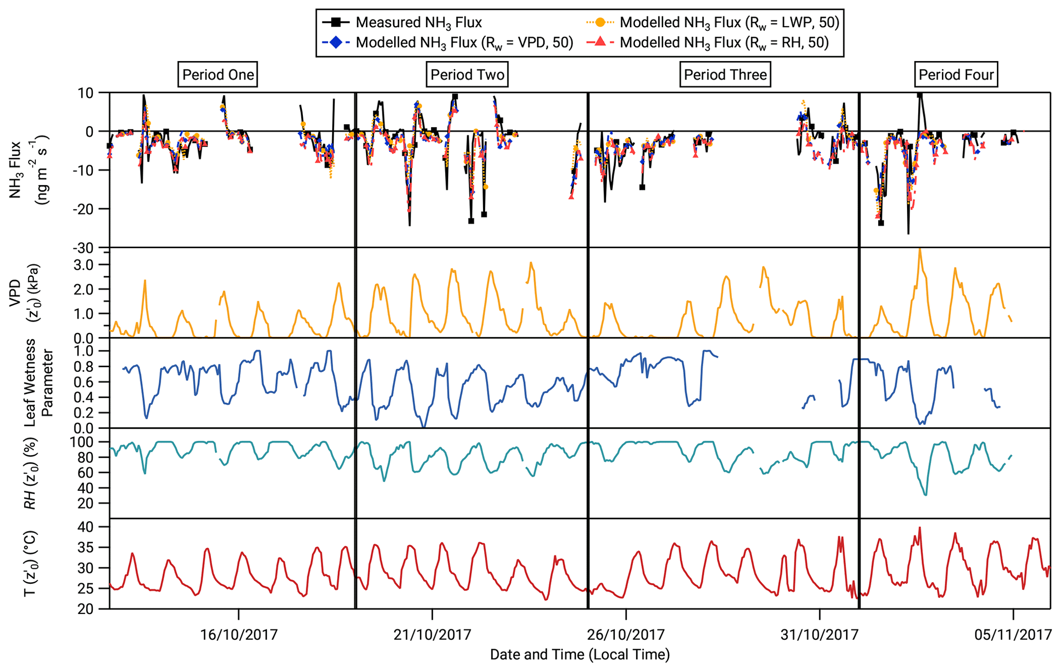
Figure 2 Time series of (from top to bottom) measured and modelled NH₃ fluxes, vapour pressure deficit at $z_{\mathrm{0}}^{\prime }$, leaf wetness parameter, relative humidity at $z_{\mathrm{0}}^{\prime }$, and air temperature at $z_{\mathrm{0}}^{\prime }$ throughout the period of NH₃ flux measurements.

A distinct lag exists between the relative humidity at the canopy level and the leaf wetness measurements, particularly during the drier conditions from 19 to 25 October. RH minima, which occur on average between 11:00 and 13:00 (all times presented in this work are given as local time: Amazon time, UTC−4), are not reflected in leaf wetness measurements until several hours later. Minima leaf wetness measurements during this period are recorded between 13:00 and 16:00.

3.2 Overview of NH₃ measurements

Figure 2 shows the time series of the measured fluxes together with model results (see below). Both (positive) emission and (negative) deposition fluxes were recorded during the campaign, ranging from +9.5 to − 30.2 $\mathrm{ng}{\mathrm{m}}^{-\mathrm{2}}{\mathrm{s}}^{-\mathrm{1}}$. Figure 3 presents calculated NH₃ fluxes as scatter plots for the duration of the campaign against paired canopy values of temperature and relative humidity as well as the leaf wetness parameter. Shaded contour areas – from green to red for low to high density of measurements – are added to the scatter plots to highlight temperature, relative humidity, and leaf wetness conditions where measurements of NH₃ fluxes were particularly concentrated. A statistical summary of linear regression models for calculated NH₃ flux and the respective parameter plotted is given for each subplot in Fig. 3.

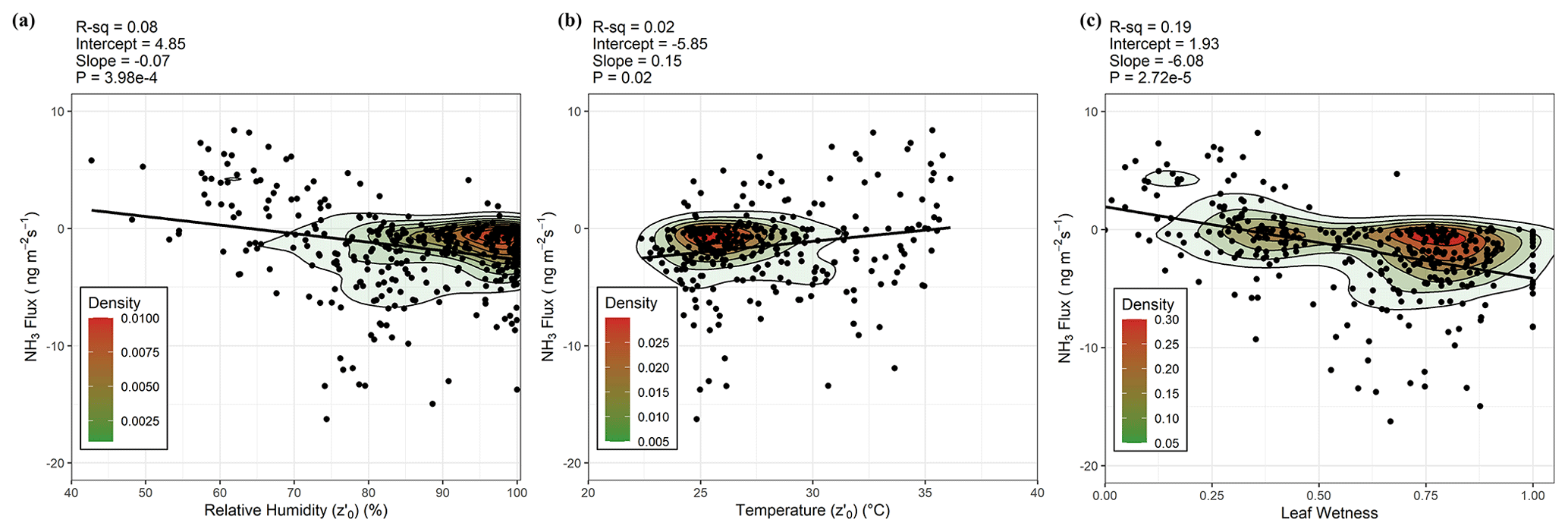
Figure 3 Scatter plots with line of best fit and data density shadings for NH₃ flux against (from a to c) relative humidity at $z_{\mathrm{0}}^{\prime }$, temperature at $z_{\mathrm{0}}^{\prime }$, and leaf wetness parameter.

While emission and deposition occur across the full range of temperatures recorded during the campaign, a weak correlation (R²=0.02; p=0.02) in the linear regression model of NH₃ flux against temperature suggests that emissions were more likely to be observed during warmer conditions. Relative humidity appears to be a somewhat stronger driver of NH₃ surface exchange behaviour (R²=0.08; $p=\mathrm{3.98}\times {\mathrm{10}}^{-\mathrm{4}}$) than temperature. The slope and density contours suggest that emissions are more likely as relative humidity decreases. The strongest predictor of the three meteorological parameters investigated is the leaf wetness parameter (R²=0.19; $p=\mathrm{2.72}\times {\mathrm{10}}^{-\mathrm{5}}$). Emissions predominately occur during periods when leaf wetness parameter values fall below 0.5, with deposition occurring predominately during periods when the leaf surface is wet (> 0.6) or completely saturated 1 (Fig. 2).

3.3 Determination of stomatal compensation points and emission potentials

One of the elements of modelling of NH₃ flux through the static canopy compensation point model is the stomatal flux (F_s), which, from Eq. (11), depends on the canopy concentration of NH₃ (χ_c) and the stomatal compensation point (χ_s). The value of χ_s is determined by the leaf surface temperature (in this study, taken as $T_{z_{\mathrm{0}}^{\prime }}$) and the apoplastic ratio (Γ_s). If Γ_s is known, which varies with vegetation type (Hoffmann et al., 1992; Mattsson et al., 2009), environmental stressors such as drought (Sharp and Davies, 2009), and nitrogen nutrition (Massad et al., 2008), then χ_s and subsequently F_s can be modelled. The fact that emissions at this site regularly occurred during midday (when $T_{z_{\mathrm{0}}^{\prime }}$ is at its maximum) and were related to drier, warmer conditions (Fig. 3) is consistent with the emission flux originating from the stomata.

Γ_s can be inferred from measurements during conditions where the NH₃ surface exchange is judged to be dominated by stomatal exchange, with a negligible contribution from desorption of NH₃ from the leaf surface.

Under conditions where R_w is very large compared with R_s, the ambient NH₃ concentration (χ_a) at which a zero net flux occurs (i.e. when the difference between χ_c and χ_s is 0) is implicitly equal to χ_c and χ_s. Therefore, if NH₃ surface exchange is driven by stomatal exchange, χ_s may be determined from the values of χ_a at which the flux changes from deposition to emission, or vice versa (Nemitz et al., 2004). Figure 4 presents the ambient NH₃ concentrations measured during the campaign at which such flux sign changes occur as a function of $T_{z_{\mathrm{0}}^{\prime }}$ for conditions under which R_w is expected to be fairly large (RH < 60 %).

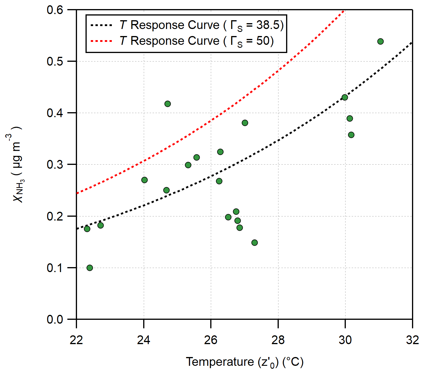
Figure 4 Estimating the stomatal compensation point from the ambient NH₃ concentrations at which the flux changed signs as a function of the temperature at $z_{\mathrm{0}}^{\prime }$. The black dotted line shows the temperature response curve calculated using an apoplastic ratio of 38.5, while the red dotted line shows the temperature response curve calculated using a ratio of 50.

Equation (12) can therefore be rearranged to give an expression for Γ_s that is dependent upon $T_{z_{\mathrm{0}}^{\prime }}$ and χ_s, where χ_s can be substituted with a value of χ_a at which a sign change in the flux of NH₃ occurs:

$$\begin{array}{}\text{(16)}& {\mathrm{\Gamma }}_{\mathrm{s}}={\displaystyle \frac{\mathrm{1}}{\left[\frac{\mathrm{161500}}{T_{z_{\mathrm{0}}^{\prime }+\mathrm{273}}}\exp \left(-\frac{\mathrm{10380}}{T_{z_{\mathrm{0}}^{\prime }+\mathrm{273}}}\right)\left(\frac{\mathrm{1}}{{\mathit{\chi }}_{\mathrm{s}}}\right)\right]}}.\end{array}$$

Using the values of χ_a measured in this campaign that are inferred to be equal to χ_s, the apoplastic ratio applicable to the period of measurement was determined as 38.5 ± 15.8. Also shown in Fig. 4 is the temperature response curve of χ_s consistent with this value of Γ. Consequently, modelled values of χ_s based on a value of Γ_s=38.5 were determined for the campaign period and subsequently used to determine values of χ_c and total modelled flux. As this value resulted in an under-prediction of the peak emissions, an alternative enhanced value of Γ_s=50 was also explored to develop further parameterisations for comparison. By using an enhanced value for Γ_s, all emissions from the leaf surface are implicitly considered to originate from leaf stomata rather than cuticular desorption or other potential sources of NH₃ emissions, such as soil or leaf litter.

3.4 Determination of R_w parameterisations based on three alternative proxies for leaf water volume

Considering the observed drivers for NH₃ surface exchange discussed in Sect. 3.2, three different parameterisations for the cuticular resistance R_w were developed for this study, based upon three alternative proxies of the NH₃ holding capacity of the leaf water layers: RH${}_{z_{\mathrm{0}}^{\prime }}$, $VP{D}_{z_{\mathrm{0}}^{\prime }}$, and leaf wetness. Subsequently, each parameterisation of R_w was used to develop three distinct values for F_w, the unidirectional flux component of the cuticular-resistance-based single-layer model, each describing the surface atmosphere exchange of NH₃ at the ATTO site.

The first parameterisation was based on measurements of RH${}_{z_{\mathrm{0}}^{\prime }}$ using the following equation (Sutton et al., 1993):

$$\begin{array}{}\text{(17)}& R_{\mathrm{w}}=\mathit{\alpha }+\exp \left({\displaystyle \frac{\mathrm{100}-\mathrm{RH}}{{\mathit{\beta }}_{\mathrm{1}}}}\right).\end{array}$$

Here, α determines the minimum cuticular resistance (which is α=1 s m⁻¹), while β₁ is a constant scaling coefficient controlling the increase of R_w with decreasing relative humidity. The coefficients α and β₁ were fitted by least-squares optimisation between total modelled and observed values of NH₃ flux taken during the campaign to arrive at values of α=2 s m⁻¹ and β₁=9, which were used for modelling R_w based on RH${}_{z_{\mathrm{0}}^{\prime }}$ for the entirety of the campaign. The second parameterisation was based on measurements of the vapour pressure deficit, using a formulation for R_w based upon that employed by Flechard et al. (1999):

$$\begin{array}{}\text{(18)}& R_{\mathrm{w}}=\mathit{\alpha }+{\mathit{\beta }}_{\mathrm{2}}\left({\exp }^{{\mathit{\gamma }}_{\mathrm{1}}\left(\mathrm{VPD}\right)}\right).\end{array}$$

As with the parameterisation of R_w in Eq. (17), the coefficient α is the minimum value for R_w at zero VPD, set at 2 s m⁻¹. β₂ and γ₁ are constant scaling coefficients which, respectively, control the scaling of the exponential term and the scaling of the vapour pressure deficit response. Through least-squares optimisation, a value of 5 was chosen for β₂ and 1.7 for γ₁ for the determination of R_w based on Eq. (18) for the entirety of the campaign.

Finally, a novel parameterisation for R_w based upon measurements of leaf wetness was developed for this campaign based on least-squares optimisation:

$$\begin{array}{}\text{(19)}& R_{\mathrm{w}}=\mathit{\alpha }+{\mathit{\beta }}_{\mathrm{3}}\left[{\exp }^{{\mathit{\gamma }}_{\mathrm{2}}(\mathrm{1}-LWP)}-\mathrm{1}\right].\end{array}$$

As with the parameterisations of R_w described in Eqs. (17) and (18), α is the minimum value of R_w at maximum leaf wetness, set at 2 s m⁻¹; β₃ is a scaling coefficient, similar to that of the parameterisation in Eq. (18), set at a value of 5; and γ₂ is a scaling coefficient controlling the increase in R_w with the decrease in leaf wetness, set in this study to 4.8. With this parameterisation, R_w approaches α for a fully wet canopy and is capped at R_w=605 s m⁻¹ for a fully dry canopy.

3.5 Comparison of modelled with observed NH₃ fluxes

Six discrete model runs of NH₃ surface exchange were investigated, via Eqs. (9), (10), and (11), using the two values of the apoplastic ratio (Γ_s=38.5 and Γ_s=50) combined with one of the three parameterisations for R_w (relative humidity, RH; vapour pressure deficit, VPD; and leaf wetness parameter, LWP) described above. These models are

• a.

  R_w= LWP, Γ_s=38.5,

• b.

  R_w= LWP, Γ_s=50,

• c.

  R_w= RH, Γ_s=38.5,

• d.

  R_w= RH, Γ_s=50,

• e.

  R_w= VPD, Γ_s=38.5, and

• f.

  R_w= VPD, Γ_s=50.

Table 1 presents a summary of the model results, with average mean modelled fluxes for the overall campaign, together with day- (06:00–17:00) and night-time (18:00–05:00) average mean values for the four separate periods of the campaign discussed in Sect. 3.1. Also presented are average mean values for calculated fluxes based on NH₃ measurements during the campaign and the percentage of modelled values which agree in flux direction with observed values. Modelled mean values highlighted in bold signify where the model value deviates by more than 25 % from the corresponding observed mean. The models which differ least and most from the observed values are models b and c, respectively. Models which use the calculated apoplastic ratio of 38.5 differ more from the observed values than those which use an apoplastic ratio of 50 (near 1 standard deviation from calculated). Modelled daytime values tend to differ less from their corresponding observed value in comparison to night-time values. Modelled values during Period One have the least divergence from the observed overall (day and night), while the greatest divergence in modelled values occurs during Period Four, particularly at night. For model b, 91 % of values agree with the observed direction of fluxes, and it is the best performing model using this parameter. Conversely, model c values agree with only 83 % of the observed direction of fluxes.

Table 1 Summary of model results, with comparison to measured hourly NH₃ fluxes (in $\mathrm{ng}{\mathrm{m}}^{-\mathrm{2}}{\mathrm{s}}^{-\mathrm{1}}$). Presented are the overall mean average flux for measured and modelled NH₃ fluxes (with associated errors), the correctness of modelled flux direction in comparison to the measured values, and mean average values for modelled and measured NH₃ fluxes during day (06:00–17:00) and night (18:00–05:00) for the four periods of the measurement campaign. Values in bold signify average model values which differ by ± 25 % from corresponding measured average values.

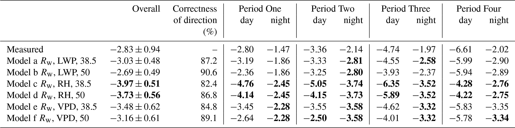
Figure 2 shows the full time series of modelled NH₃ fluxes from models b, d, and f alongside the measured flux. In general, periods of emission and deposition are modelled well by all three models, with two exceptions: the emission period from 12:00 to 16:00 on 30 October, where modelled fluxes suggest an earlier emission from 11:00 which lasts for fewer hours; and from 13:00 to 15:00 on 2 November, where no model predicts an emission, in contrast to the measurements. The magnitude of modelled fluxes generally agrees well with the observed flux, although model d, which uses an R_w parameterisation based on RH, tends to estimate smaller emissions in comparison to model f (R_w= VPD). Model b (R_w= LWP) comes closest to replicating the magnitudes of the measured emissions, although as with the other two models it underestimates the magnitude of the measured deposition.

3.6 Error in observed and simulated fluxes

The errors in the observed fluxes of NH₃ during this campaign are presented in Ramsay et al. (2020). Using a Gaussian error propagation approach, a median percentage error of 33 % was calculated for the observed NH₃ fluxes.

The error in the simulated fluxes can also be determined using an error propagation method. Equation (9) highlights that the total simulated flux (F_t) is the sum of the cuticular flux (F_w) and the stomatal flux (F_s). The total uncertainty in F_t, ${\mathit{\sigma }}_{F_{\mathrm{t}}}$, can therefore be determined by

$$\begin{array}{}\text{(20)}& {\mathit{\sigma }}_{F_{\mathrm{t}}}=\sqrt{{{\mathit{\sigma }}_{F_{\mathrm{w}}}}^{\mathrm{2}}+{{\mathit{\sigma }}_{F_{\mathrm{s}}}}^{\mathrm{2}}},\end{array}$$

where ${\mathit{\sigma }}_{F_{\mathrm{w}}}$ and ${\mathit{\sigma }}_{F_{\mathrm{s}}}$ are the associated errors in, respectively, F_w and F_s. In turn, ${\mathit{\sigma }}_{F_{\mathrm{w}}}$ and ${\mathit{\sigma }}_{F_{\mathrm{s}}}$ can be calculated using a Gaussian error propagation based on Eqs. (10) and (11) respectively, which rely on the errors in R_a, R_b, R_s, and R_w measurements.

While the error in F_s will remain the same for all simulated values of F_t, the error in F_w will vary on the choice of R_w parameterisation. Thus, the error in R_w is the primary variable which governs the differences in the error in F_t between the simulated values.

Using this framework, the error values were calculated for each R_w and Γ_s parameterisation for the simulated total flux. In the overall calculated total flux in Table 1, the associated error, in $\mathrm{ng}{\mathrm{m}}^{-\mathrm{2}}{\mathrm{s}}^{-\mathrm{1}}$, is also shown.

4 Discussion

4.1 Temporal dynamics

The observed bidirectional surface exchange of NH₃ from a remote tropical rainforest site was modelled using a series of canopy compensation point, cuticular-resistance-based models using a variety of different R_w parameterisations and apoplastic ratios.

As highlighted in the Introduction, measurements of NH₃ surface exchange over natural ecosystems such as forests remain sparse. This is particularly true for measurements over remote environments such as tropical vegetation. To our knowledge, there have not been any direct flux measurements over tropical vegetation to date, although Trebs et al. (2004) and Adon et al. (2010, 2013) inferred fluxes from single point concentration measurements. Exchange of NH₃ has been measured previously at temperate forest sites and reported to be bidirectional: for example, Langford and Fehsenfeld (1992) noted daytime emission from a remote forest near Boulder, Colorado; Neirynck and Ceulemans (2008) observed bidirectional NH₃ exchange (with median diel emissions recorded between 12:00 and 16:00) over a Scots pine (Pinus sylvestris) forest in Flanders, Belgium; and Wyers and Erisman (1998) noted daytime emissions from a Douglas fir (Pseudotsuga menziesii) forest at Speuld in the Netherlands. When using models to determine the drivers of surface exchange above forest sites, these studies often stress the importance of cuticular desorption as a further process that dominated in the morning when emission could not have originated from stomatal compensation points. Indeed, in the case of Neirynck and Ceulemans (2008), the static canopy compensation point model (SCCP) was unable to simulate their observed emissions.

At ATTO, there is no indication that the single-layer SCCP model was unable to reproduce the temporal dynamics of the measured NH₃ surface exchange. Indeed, an exploratory application of the dynamic CCP model did not result in an improvement in model performance, and therefore the modelling work here focused on the static model as a simpler approach able to reproduce the measurements. The absence of morning desorption peaks at the ATTO forest is likely due to the small night-time adsorption of NH₃ into leaf water layers associated with the low night-time NH₃ concentrations at this site. Dry deposition of aerosol ammonium nitrate (NH₄NO₃) is another source of volatile ${\mathrm{NH}}_{\mathrm{4}}^{+}$ on leaf surfaces, and concentrations of this compound are again typically very small in Amazonia (Wu et al., 2019). In addition, given the high RH, the water layers may not dry out as rapidly and completely as at other sites. The measured median NH₃ atmospheric concentration at the canopy height during the measurement period was 0.23 µeq m⁻³, with an estimated annual total reactive N dry deposition input of 1.74 kg N ${\mathrm{ha}}^{-\mathrm{1}}{\mathrm{yr}}^{-\mathrm{1}}$ (Ramsay et al., 2020). This is far lower than reported by Neirynck and Ceulemans (2008) and by Wyers and Erisman (1998), both of whose sites were subject to high levels of agricultural pollution. As noted by Massad et al. (2010) and Zhang et al. (2010), higher atmospheric inputs of N to forest systems lead to an increase in the stomatal emission potential. Conversely, with lower atmospheric NH₃ concentrations, the potential for forests to act as a source of NH₃ is increased, as the likelihood of the canopy compensation point exceeding the ambient concentration increases. The low N status of the tropical vegetation may also favour transfer of N absorbed to the cuticle into the leaf, e.g. via liquid films that extend from the cuticle into the stomata (Burkhardt et al., 2012).

In general, the fluxes measured at ATTO could also be reproduced without including a further soil layer, potentially with one exception (see below). Such a layer is needed where night-time emissions are observed that are clearly not under stomatal control (Nemitz et al., 2000; Hansen et al., 2017).

The consistently warmer noon-time conditions at the leaf canopy during measurements at the ATTO site would also favour stomatal-exchange-driven emissions of NH₃. An increase in leaf temperature, with VPD controlled for, has been shown to lead to greater gas exchange through increased stomatal openings (Urban et al., 2017), while alterations to the Henry and dissociation equilibria would lead to a change in the stomatal compensation point favouring increased stomatal emissions. Similarly, the unstable conditions at noon above the canopy over tropical rainforest lead to reductions in R_a, which would increase any emissions occurring at the time that were driven by stomatal exchange (Flechard et al., 2015). In the study of forest NH₃ emissions that is most similar in ambient NH₃ concentrations, canopy compensation points, and apoplast ratios to this study, Hansen et al. (2017) come to a similar conclusion on the observed daytime emissions from a remote, temperate forest in Indiana, USA.

Despite the low N inputs and apoplastic ${\mathrm{NH}}_{\mathrm{4}}^{+}$ $/$ H⁺ ratio, significant emission periods were observed above the ATTO site. One driver is clearly the high daytime leaf temperature. The average flux amounted to a small deposition of − 2.8 $\mathrm{ng}{\mathrm{m}}^{-\mathrm{2}}{\mathrm{s}}^{-\mathrm{1}}$ suggesting that, on average, the site receives more N as NH₃ than it loses. Possible sources include small-scale farming and biomass burning.

4.2 Apoplast ratio

The apoplastic ratio of ${\mathrm{NH}}_{\mathrm{4}}^{+}$ $/$ H⁺ (Γ_s) inferred from the measurements in this study was 38.5 ± 15.8; the models investigated used either a value of 38.5 or 50 (close to 1 standard deviation from inferred value). Both values are significantly lower than the majority of Γ_s values obtained for other forest sites. Wang et al. (2011) give a value of Γ_s=400 for green temperate forest canopies, which is also used by Hansen et al. (2017). Massad et al. (2010) review a range of Γ_s values derived from measurements of NH₃ surface exchange over forest, which range from Γ_s = 27 (as measured directly through bioassay for unfertilised Spruce forest) to Γ=5604 as determined by Wyers and Erisman (1998) for a highly polluted P. menziesii forest. The study by Neirynck and Ceulemans (2008) used a value of 3300 in spring and 1375 in summer for a P. sylvestris forest.

The disparity in the emission potentials (the apoplastic ratios) between other forest sites and the tropical rainforest site at ATTO is again linked to nitrogen input. With larger N inputs where nitrogen is deposited in excess, the stomatal concentration is increased (Schjoerring et al., 1998). Consequently, at polluted areas such as the forest sites studied by Neirynck and Ceulemans (2008), apoplastic ratios are increased, while at sites with lower N input, such as semi-natural vegetation with low ambient NH₃ concentrations, values of Γ_s can be as low as 5–10 (Hanstein et al., 1999). The species of vegetation is also critical (Mattsson et al., 2009). Plants which are reliant on mixed nitrogen sources (ammonium, nitrate, and organic N), and which are more reliant on root rather than shoot assimilation of nitrogen, exhibit lower apoplast ratios than nitrate-reliant, shoot-assimilating species (Hoffmann et al., 1992). The value of 38.5 which was inferred from measurements lies in the range of Γ_s values exhibited by semi-natural vegetation with low N inputs and in the lower range of overall forest values quoted by Massad et al. (2010).

4.3 Model performance with respect to R_w parameterisation

An assessment of the performance of the individual parameterisations against calculated NH₃ fluxes is included in Fig. 5, which displays the results of simple linear regression models for the simulated values of each NH₃ flux model against observed NH₃ fluxes. With regards to the Pearson correlation coefficient (r), the rank of models from most strongly correlated with observed NH₃ fluxes to least correlated is model b, model a, model f, model e, model d, and model c (model descriptions are found in Table 1). The R_w parameterisation was a stronger determinant of model–measurement correlation than the choice of Γ. Correlation with measurements is highest for the models using an R_w based upon LWP, followed by those which use VPD and finally RH. Within each grouping, models using Γ=50 provide simulated values that have a better correlated fit with observed values than Γ=38.5. Overall model performance is in many ways more sensitive to R_w than Γ as is apparent from the Taylor diagram (Fig. 6), which summarises in one diagram the three complementary model–measurement performance statistics of the (i) correlation coefficient (r), (ii) centred root mean squared error (RMSE), and (iii) within-model and within-measurement standard deviations (SD) (Taylor, 2001). The statistical metrics visualised in Fig. 6 are summarised in Table 2.

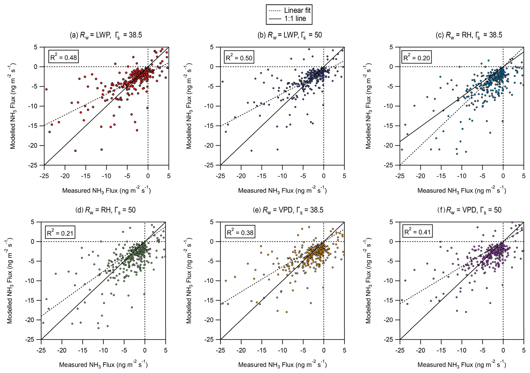
Figure 5 Linear regressions between measured NH₃ fluxes and six models (a–f) of NH₃ fluxes differing in the approach used to derive a value for the cuticular resistance R_w and in the value used for the apoplastic ratio Γ, as noted above each panel.

The standard deviation in the observed flux dataset is 3.65 $\mathrm{ng}{\mathrm{m}}^{-\mathrm{2}}{\mathrm{s}}^{-\mathrm{1}}$. The model that comes closest to replicating this same variability is model b (2.65 $\mathrm{ng}{\mathrm{m}}^{-\mathrm{2}}{\mathrm{s}}^{-\mathrm{1}}$), with model e (2.24 $\mathrm{ng}{\mathrm{m}}^{-\mathrm{2}}{\mathrm{s}}^{-\mathrm{1}}$) replicating observed values least well, although the overall range between model standard deviation is broadly similar. It should be borne in mind, however, that the standard deviation of the measured flux includes measurement uncertainty in addition to real variability, as do the modelled values, which are based on measured parameters. With regards to r, model b simulated values produce the highest correlation with the observed values at r=0.71, in comparison to model c, which performs the worst at r=0.45. Finally, the model with the lowest root mean square error from the observed is model b at 2.79 $\mathrm{ng}{\mathrm{m}}^{-\mathrm{2}}{\mathrm{s}}^{-\mathrm{1}}$, with the highest error found in model c, at 3.31 $\mathrm{ng}{\mathrm{m}}^{-\mathrm{2}}{\mathrm{s}}^{-\mathrm{1}}$. Therefore, from the ability of the parameterisations to reproduce the measured average fluxes as presented in Figs. 5, 6, and (Table 1), it can be concluded that parameterisation b, in which the value R_w is parameterised using leaf wetness parameter values and where the apoplastic ratio is set to 50, is the best performing model in simulating NH₃ surface–atmosphere exchange at the ATTO site, while model c is the worst performing.

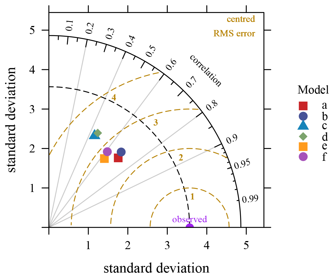
Figure 6 A Taylor diagram summarising the statistical comparisons between the modelled NH₃ fluxes from the six models a–f described in the text and the measured NH₃ fluxes.

Table 2 Summary of model statistical performance (correlation coefficient R, centred root mean square error, and standard deviation) as presented in Fig. 6.

Although the leaf wetness parameter measured with the leaf clip sensors is somewhat empirical, it is not surprising that it appears to reflect the actual leaf water amount more closely than the proxies via VPD and RH. All three parameters should be closely linked. Even after optimisation of the models, however, extensive differences in model output remain, principally between the models using leaf wetness parameter and RH as model inputs. Figure 7 presents a scatter plot of leaf wetness measurements against RH normalised to the canopy height. The relationship between them is best described through a power equation, which suggests that leaf wetness decreases more sharply than RH across the campaign. Indeed, Fig. 2 shows a distinct lag between observed RH (as well as VPD) and the leaf wetness parameter. While RH minima are detected between 11:00 and 13:00, and ranges in a fairly narrow band between 100 % and 80 %, leaf wetness reaches minima between 13:00 and 16:00 and can decrease significantly, particularly during Period Two of the campaign.

Overall, the results indicate that there is significant value for interpreting field measurements in making direct measurements of leaf wetness using leaf wetness clip sensors of the type used here. Although leaf wetness or surface wetness measurements are not typically available for use in chemistry transport models, canopy wetness is often simulated by land surface models (Katata et al., 2010) and within chemical transport models (Campbell et al., 2019). Simulated surface wetness data, as a leaf wetness parameter, could therefore be used to model NH₃ fluxes using the LWP-dependent R_w parameter as described here. Alternatively, VPD-based parameterisations, over RH-based parameterisations, could be employed instead.

4.4 Model performance with respect to the choice of stomatal emission potential

As is visually apparent in Fig. 7, the influence of the apoplastic ratio is relatively minimal for reproducing flux variability in comparison to the effect of R_w parameterisation over the Γ_s range explored (38.5 to 50). However, the choice of Γ does affect the model's ability to reproduce the overall magnitude of the fluxes during daytime (Table 2).

Models that used the Γ_s value of 50 (the upper bound to the inferred values of 38.5 for Γ_s) (b, d, and f) simulated values better in agreement with observations in comparison to their paired R_w models (respectively, a, c, and e) which used the value of 38.5. In particular, the use of 38.5 as a value led to models underestimating the scale of the emissions.

The discrepancy highlights a potential problem with using the method of inferring Γ_s as outlined in Sect. 3.3 in tropical conditions. As outlined by Nemitz et al. (2004), the validity of equating χ_a to χ_c only holds for dry conditions (e.g. RH < 50 %), when R_w can reliably be expected to be large. At higher humidity values, leaf cuticles may start to become a small sink, and χ_c becomes an underestimate of χ_s. At the ATTO site, where median humidity at the canopy level throughout the campaign was 87 %, with only a few occurrences during the drier Period Two and Period Four where it fell below 60 %, this approach of inferring Γ_s from NH₃ measurements was likely affected. However, the impact does not appear to have completely invalidated the use of the method, as the somewhat larger value of 50 that resulted in models with best agreement still lies within 1 standard deviation of the inferred Γ_s value. An accurate determination of apoplastic ratio for tropical rainforest, derived from leaf assays, would improve the accuracy of the model and therefore remains an important area for future investigation. However, its variability across the large plant species diversity would likely provide a challenge in deriving a bottom-up mean value that governs the net exchange.

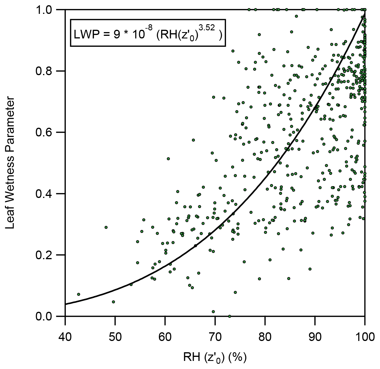
Figure 7 Scatter plot of hourly leaf wetness parameter and relative humidity $z_{\mathrm{0}}^{\prime }$ measurements taken during campaign, with a fitted power relationship.

4.5 Temporal variability in model performance

Modelled values diverge significantly from observations at several points during the campaign. In particular, on 30 October every model predicts an earlier, less sustained emission in comparison to the observation, while on 2 November, no model predicts any emission, contrary to observations, which suggest a strong emission of NH₃ from 13:00 to 15:00. With regards to the divergence in models from the observations on 2 November, the possibility of other sources of NH₃ emission that would not be accounted for using the single-layer model could be considered. For example, from the evening of 31 October to the early morning of 2 November, heavy precipitation periods were recorded, coupled with increased deposition fluxes of NH₃ on 1 November. Increased wet deposition of N through ${\mathrm{NH}}_{\mathrm{4}}^{+}$ in rainwater and washed from the canopy (Nemitz et al., 2000) to the forest floor or the higher soil moisture itself could have led to an increase in soil or leaf litter microbial activity below canopy. Subsequent drying of the soil and leaf litter throughout 2 November might have led to an evaporation of NH₃ from the litter or soil layer from the forest floor (Hansen et al., 2017), leading to observed emissions of NH₃ in the afternoon. This potential scenario would not be modelled with the single-layer canopy resistance model.

Average modelled values for daytime tended to agree better with their corresponding period of observations than night-time values. Overall, the six models tended to overestimate nocturnal NH₃ deposition, particularly during Period Two and Four when all six models overestimated the average deposition by more than 25 % from the corresponding average observations. Of course, the flux measurement itself is not without error, especially during the calmer and more stable night-time conditions.

5 Conclusions

Observations of the bidirectional surface–atmosphere exchange of NH₃ at a tropical rainforest site have been successfully replicated using a static single-layer resistance model. Application of a capacitance model that additionally incorporates the process of cuticular desorption did not lead to improved model results, suggesting that the emission periods were under stomatal control. Models that used a single-layer canopy resistance approach, where the cuticular resistance was governed either by RH, VPD, or a measurement of leaf wetness, were able to replicate the pattern of observed NH₃ deposition with frequent periods of afternoon emissions. Of all the models used, the most successful was a cuticular resistance modelling approach based on using leaf wetness measurements and where modelled χ_c was governed by an apoplast $\mathrm{\Gamma }={\mathrm{NH}}_{\mathrm{4}}^{+}/{\mathrm{H}}^{+}$ ratio of 50, 1 standard deviation above the mean inferred from the measurements.

The periods when the most frequent emissions of NH₃ occurred, and which were most successfully modelled by cuticular resistance models, are typified by conditions that diverge from the overall campaign average, i.e. above-average temperatures and below-average relative humidity. This campaign took place in the dry season, and so comparison with the surface exchange of NH₃ during the wet season would be a necessary first step in determining if stomatal exchange is the principal driver of NH₃ surface exchange throughout the year. Long-term observations would also be required to determine whether the temperature increases, whether drought conditions and elevated ambient NH₃ concentrations that are anticipated from climate change and human development over this region have any impact on NH₃ surface exchange, and whether prolonged reactive nitrogen input from biomass burning activities raise compensation points.

One outcome of this study has been to establish the suitability of leaf wetness measurements, converted to a suitable parameter, as a factor for modelling cuticular resistance in NH₃ surface exchange modelling. Leaf wetness measurements, albeit from wetness grid sensors, have been used previously in NH₃ modelling, but these were first converted to an associated value of RH before being used in RH-based R_w parameterisations. Using leaf contact sensors, this study demonstrates that leaf wetness can be used directly with a R_w parameterisation that here proved to be the most sensitive and accurate in simulating cuticular NH₃ exchange.

A Γ value of 50 led to the best modelling of χ_c values and hence to the best fit with observed values. While within 1 standard deviation from the initially inferred value of 38.5, this did highlight that the method used to infer apoplastic ratio perhaps suffered under the high-humidity conditions present at the rainforest site. An accurate determination of emission potential for this region is required for global-scale modelling, necessitating accurate measurements of the apoplast ratio, i.e. the use of leaf assays to determine Γ_s. Future studies of NH₃ surface exchange above rainforest should therefore seek to incorporate accurate determinations of leaf apoplastic ratio as a necessary part of their methodology.

Some periods of divergence between the models and observed values highlight that other sources of NH₃ surface exchange (such as soil or leaf litter exchange) should be incorporated into future investigation, while also emphasising the difficulty in measuring and modelling NH₃ surface exchange in remote, challenging conditions. A complete understanding of NH₃ surface exchange dynamics at rainforest sites will require a full suite of instruments measurements, incorporating in-canopy measurements of NH₃ concentration gradients, trunk space flux measurements, and characterisation of leaf and soil ${\mathrm{NH}}_{\mathrm{4}}^{+}$ pools.