Coastal processes modify projections of some climate-driven stressors in the California Current System

Global projections for ocean conditions in 2100 predict that the North Pacific will experience some of the largest changes. Coastal processes that drive variability in the region can alter these projected changes but are poorly resolved by global coarse-resolution models. We quantify the degree to which local processes modify biogeochemical changes in the eastern boundary California Current System (CCS) using multi-model regionally downscaled climate projections of multiple climate-associated stressors (temperature, O₂, pH, saturation state (Ω), and CO₂). The downscaled projections predict changes consistent with the directional change from the global projections for the same emissions scenario. However, the magnitude and spatial variability of projected changes are modified in the downscaled projections for carbon variables. Future changes in pCO₂ and surface Ω are amplified, while changes in pH and upper 200 m Ω are dampened relative to the projected change in global models. Surface carbon variable changes are highly correlated to changes in dissolved inorganic carbon (DIC), pCO₂ changes over the upper 200 m are correlated to total alkalinity (TA), and changes at the bottom are correlated to DIC and nutrient changes. The correlations in these latter two regions suggest that future changes in carbon variables are influenced by nutrient cycling, changes in benthic–pelagic coupling, and TA resolved by the downscaled projections. Within the CCS, differences in global and downscaled climate stressors are spatially variable, and the northern CCS experiences the most intense modification. These projected changes are consistent with the continued reduction in source water oxygen; increase in source water nutrients; and, combined with solubility-driven changes, altered future upwelled source waters in the CCS. The results presented here suggest that projections that resolve coastal processes are necessary for adequate representation of the magnitude of projected change in carbon stressors in the CCS.

1 Introduction

Greenhouse gas emissions have imparted large physical and biogeochemical modifications on the world's oceans (Friedlingstein et al., 2019; Gattuso et al., 2015; Le Quéré et al., 2018). The oceans have become warmer, and stratification patterns have been modified (Talley et al., 2016). These changes are occurring in tandem with biogeochemical alterations, including O₂ declines, productivity changes, and increased dissolved inorganic carbon (DIC) content due to the uptake of anthropogenic carbon dioxide (Doney et al., 2009, 2020; Feely et al., 2004, 2009). The ocean uptake of anthropogenic carbon dioxide influences the ocean's buffering capacity; reduces calcium carbonate saturation states (Ω); and lowers pH, causing a shift towards more acidity, commonly termed ocean acidification (Caldeira and Wickett, 2003; Doney et al., 2009; Feely et al., 2004, 2009; Orr et al., 2005; Sabine et al., 2004). These changing ocean conditions are occurring in both open-ocean and coastal environments, where they have the potential to impact marine organisms and ecosystems individually (Doney et al., 2012, 2020; Gattuso et al., 2015) and as interactive multi-stressors (Howard et al., 2020a; Pörtner et al., 2004; Pörtner and Knust, 2007). Big changes are happening in the ocean, but there are reasons to believe that global trends may not accurately represent what happens in coastal regions.

The majority of coastal areas have experienced significant increases in sea-surface temperature (SST) at a rate that exceeds the global average (Hartmann et al., 2013; Lima and Wethey, 2012). In contrast to most other large marine ecosystems, the coastal SST in the California Current System (CCS) has decreased over the past 3 decades (Lima and Wethey, 2012). These results suggest that global projections and trends are poor indicators of future change in SST in the CCS and that spatial variability of that change within the CCS is also possible.

As the oceans warm, they lose O₂ because the solubility of O₂ decreases with increasing temperature. However, direct solubility effects only partially explain the O₂ decline (Bopp et al., 2013; Breitburg et al., 2018). Warming impacts O₂ in other ways, for example by raising organismal metabolic rates and accelerating O₂ consumption and by increasing water column stratification and thus reducing mixing and ventilation (Breitburg et al., 2018; Deutsch et al., 2006). In coastal waters, hypoxic thresholds are more often reached than in the open ocean because of eutrophication and other local processes, such as sediment O₂ demand (Diaz and Rosenberg, 2008; Rabalais et al., 2010; Siedlecki et al., 2015). In the CCS, hypoxia already occurs regularly on the continental shelf (Adams et al., 2013; Connolly et al., 2010; Chan et al., 2008; Grantham et al., 2004), and continental slope water O₂ concentrations have been steadily declining for the past several decades (Bograd et al., 2008; Chavez et al., 2017; Deutsch et al., 2011, 2014; Pierce et al., 2012).

Atmospheric carbon dioxide has increased at a rate of 1–2 ppm yr⁻¹ (Friedlingstein et al., 2019; Le Quéré et al., 2018), and surface waters in the open ocean have effectively kept pace with the rising atmospheric concentrations over the last 30 years. Recently, the partial pressure of carbon dioxide (pCO₂) in coastal shelf waters has been shown in some places to lag the rise in atmospheric CO₂, unlike in the open ocean, which implies a tendency for enhanced shelf uptake of atmospheric CO₂, with substantial regional variability (Laruelle et al., 2018; Cai et al., 2020). One example of regional variability is found in the CCS: over the past 30 years, the CO₂ content of waters off the US west coast near Monterey Bay, CA, has increased at a rate greater than that observed in the open oceans (Chavez et al., 2017). As a result, surface water pH in Monterey Bay is on average 0.01 units lower than surface open-ocean measurements at the Hawaii Ocean Time-series due to the upwelling process and is also declining at a slightly faster rate (Chavez et al., 2017). The enhanced uptake of CO₂ over the CCS shelf amplifies the rate of acidification compared to global rates.

Local processes such as upwelling, freshwater delivery, eutrophication, water column metabolism, and sediment interactions drive biogeochemical variability on regional scales (Cai et al., 2020; Feely et al., 2008, 2016, 2018; Pilcher et al., 2018; Qi et al., 2017; Siedlecki et al., 2017). In the CCS, winds are critical for upwelling variability and are projected to strengthen in response to global warming (Bakun, 1990; Garcia-Reyes et al., 2015; Wang et al., 2015; Rykaczewski et al., 2015; Sydeman et al., 2014). The increased delivery of O₂-depleted, carbon-rich waters with enhanced nutrients and increased productivity has been projected for the CCS with a global simulation (Rykaczewski and Dunne, 2010). High-resolution projections for the CCS reinforced these findings (Dussin et al., 2019; Xiu et al., 2018) but projected that the impact of these altered conditions on productivity varied across the CCS, with an increase in the north and a decrease in the south (Xiu et al., 2018), while productivity was identified as driving the biggest change in hypoxia in the region (Dussin et al., 2019). Howard et al. (2020b) found that, while alongshore winds intensified in the future, the upwelling response was dampened by increased stratification. Global projections have coarse spatial resolution, often having only one or two grid cells for the continental shelf, and thus cannot resolve most of the local processes responsible for these observed coastal differences.

In this paper, we focus on the CCS and its known vulnerabilities to climate change by forcing regional models with the Coupled Model Intercomparison Project 5 (CMIP5; Taylor et al., 2012) simulations. We produce multi-model regionally downscaled climate projections of multiple climate-associated stressors (temperature, O₂, pH, Ω, and CO₂) that resolve coastal processes to create ∼100-year projections at resolutions of 12 and 1.5 km in the northern CCS (N-CCS). First, we quantify the surface-to-200 m depth-averaged, sea surface, and bottom condition changes for the climate stressors projected for 2100 at all resolutions (global, 12 km, and 1.5 km). Next, we use the multi-model ensemble to determine the degree to which climate-associated stressors are modified relative to global model projections of the CCS considering this signal both spatially, where the models overlap, and in different regions of the water column representative of different habitats. Finally, we interpret our results in the context of previous projections for the CCS and suggest drivers of the amplification in the downscaled projections by systematically comparing the projected changes in the winds, source waters, upwelling strengths, and coastal processes in each model system.

2 Materials and methods

2.1 Model descriptions

The downscaled regional modeling frameworks both employ the Regional Ocean Modeling System (ROMS; Shchepetkin and McWilliams, 2005). The regional models are forced with realistic atmospheric and ocean boundary conditions to make hindcast simulations as well as future projections. The model domains are shown in Fig. 1. The downscaled projections are referred to as “resolving coastal processes” because the historical simulations have been shown to represent observed coastal shelf variability. The model evaluation, provided here and available in other sources (Davis et al., 2014; Deutsch et al., 2021; Giddings et al., 2014; Siedlecki et al., 2015), indicates the downscaled models perform better spatially and temporally (seasonal and interannual) than the global models for temperature, oxygen, and carbon variables.

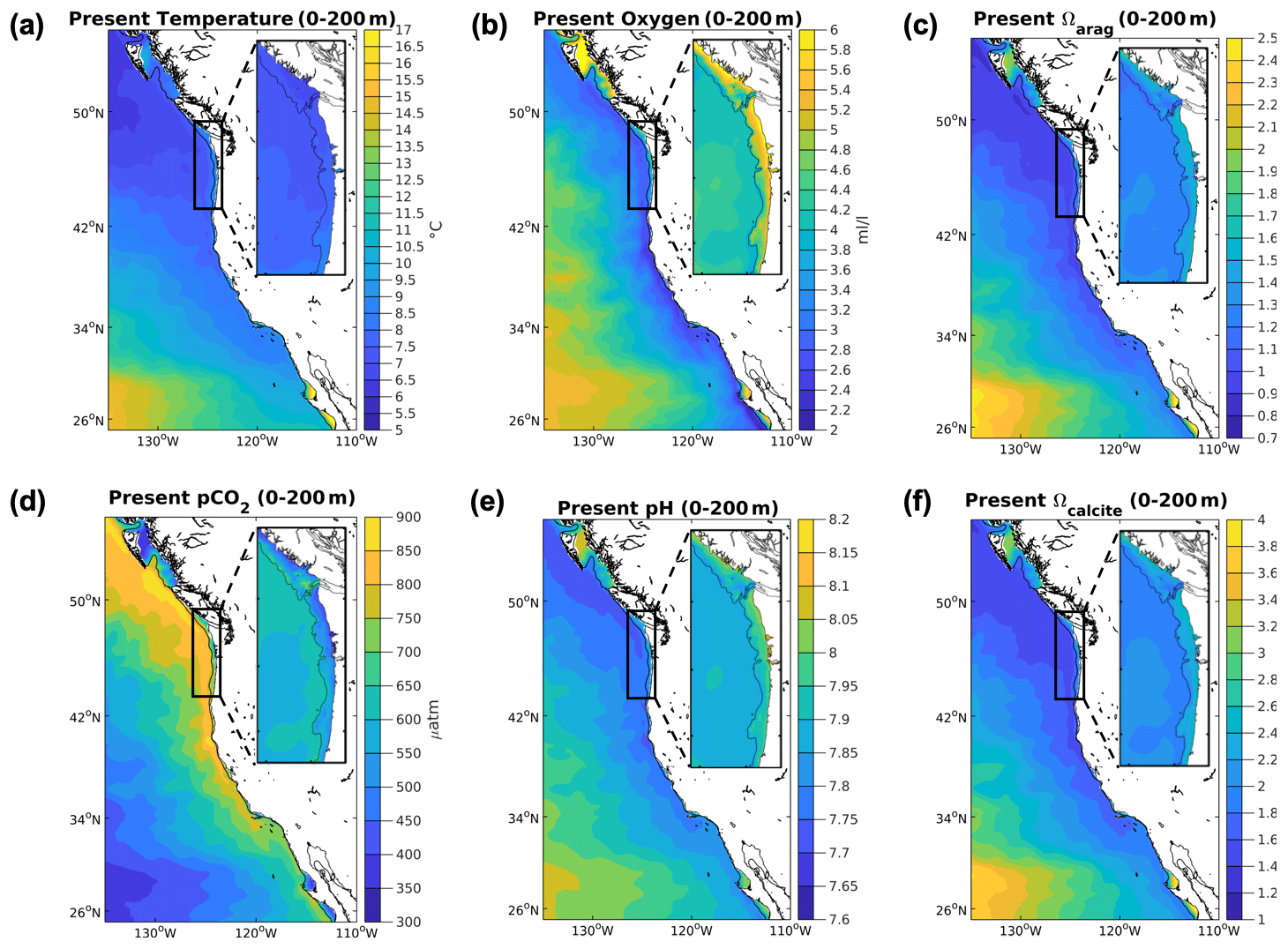
Figure 1 Base state climate stressor variables in the CCS in both domains. Depth-averaged over 200 m values for the climate stressor variables in the base state/present conditions for the 12 km (CCS-wide, full panel) and 1.5 km simulations (N-CCS, inset) for (a) temperature (^∘C), (b) O₂ (mL L⁻¹), (c) Ω_arag, (d) pCO₂ (µatm), (e) pH, and (f) Ω_calcite.

2.1.1 ∼1^∘ models

These include the CMIP model fields/global-scale model. We focus here on only the Representative Concentration Pathway 8.5 (RCP8.5) from the Earth system models (ESMs) that make up the CMIP5 modeling framework. The CMIP5 simulations include biogeochemical components described in Bopp et al. (2013). The CMIP models employed here are further described in Sect. 2.3.

2.1.2 12 km model

The mid-resolution (12 km) ROMS-based simulation of the CCS is configured for a domain that extends along the North American west coast from 25 to 60^∘ N and is described in more detail in Howard et al. (2020b). A curvilinear grid is used in the horizontal with close-to-uniform 12 km horizontal resolution and 33 s-coordinate (terrain-following vertical) levels. Atmospheric conditions including air temperature at the sea surface, precipitation, and downwelling radiation are derived from an uncoupled Weather Research and Forecasting model output (c3.6.1; Skamarock et al., 2008) as in Renault et al. (2016a, 2020), with more information in Howard et al. (2020b). To avoid the computational cost of a fully coupled ocean–atmosphere model, wind and mesoscale current feedbacks are parameterized with a linear function of the surface wind stress as in Renault et al. (2016b). This linear relationship is supported by observations in the CCS (Renault et al., 2017). The biogeochemical model is detailed in Deutsch et al. (2021) and follows Moore et al. (2004). The model has skillfully simulated the recent interannual-to-interdecadal biogeochemical variability in the CCS (Howard et al., 2020b), and a similar model setup forced with data-assimilated forcing skillfully simulated O₂ variability in the CCS over the last 2 decades (Durski et al., 2017).

2.1.3 1.5 km model

The highest-resolution (1.5 km) simulations of the N-CCS rely on a modeling framework developed by the University of Washington Coastal Modeling Group optimized for the Pacific Northwest “Cascadia” region. The Cascadia model domain encompasses the inland waters of the Salish Sea and coastal waters of the N-CCS (Fig. 1), and it includes freshwater and tidal forcing. The grid has a horizontal resolution of 1.5 km on the shelf, 4.5 km far offshore, and 40 s-coordinate (terrain-following vertical) levels, with enhanced bottom and surface resolution. The atmospheric conditions from the 12 km model are used to force the model at this resolution. The Cascadia model does not simulate biogeochemistry within the Salish Sea but yields realistic nitrate outflow from the Strait of Juan de Fuca to the outer coast shelf (Davis et al., 2014). Hindcast experiments from 2004 to 2007 were extensively validated and exhibited skill in all regions of the shelf (Davis et al., 2014; Giddings et al., 2014; Siedlecki et al., 2015).

2.2 Model metrics

Carbon variables (e.g., pH, pCO₂, and Ω) were computed using model output of DIC, total alkalinity (TA), temperature, and salinity and routines based on the standard OCMIP carbonate chemistry adapted from earlier studies (Orr et al., 2005) using CO2SYS (Lewis and Wallace, 1998). The total pH scale is used for pH throughout.

To compute model means and inter-model comparisons, first a climatological year was generated for each model grid cell, using the years 2002–2004 for the 12 and 1.5 km regional models. Then, annual average values for each cell were calculated from the climatology. Finally, spatially weighted means were calculated from the annual average values. For comparisons between model resolutions, the coarser model was interpolated to the higher-resolution model grid. For example, the global values were interpolated onto the 12 km grid prior to averaging the fields within the CCS. Surface conditions were drawn from the surface vertical layer for each simulation. Depth-averaged ocean conditions were calculated over the upper 200 m for all simulations. Where water depth was shallower than 200 m, the entire water column was averaged. For the bottom comparisons, the global simulations have a very different bathymetry than the downscaled simulations because of their coarse resolution; consequently the regional averaging efforts reported here as bottom conditions were isolated to the 0–500 m depth interval only, to ensure that the global model resolved that depth interval. We also report the downscaled values over the shelf only, limiting the determination of metrics out to the 200 m isobath.

To estimate upwelling intensity, several metrics were employed. The first two rely on the intensity of the winds (e.g., cumulative upwelling index, CUI, Schwing and Mendelssohn, 1997; 8 d wind stress, Austin and Barth, 2002); the third and fourth rely on measures in the water column itself and are referred to as the coastal upwelling transport index (CUTI) and biologically effective upwelling transport index (BEUTI) (Jacox et al., 2018). The wind-based metrics, CUI and the 8 d wind stress, are the same for both downscaled simulations, but CUTI and BEUTI are specific to each ocean model as they are calculated based on ocean measures like vertical transport and nitrate concentrations. CUTI and BEUTI were integrated over bins of 0.5^∘ latitude spanning 0–50 km offshore.

2.3 Future forcing

To generate future downscaled projections, the global CMIP5 simulations were used to force regional simulations. The methods employed are outlined below.

The 12 km historical simulation forcing is described in Renault et al. (2021) and the companion paper, Deutsch et al. (2021). The 12 km projection was forced by adding a monthly climatological difference between the CMIP5 RCP8.5 scenario forcing and the historical run forcing, averaged over 2071–2100 and 1971–2000, respectively (Howard et al., 2020b), following the delta method commonly applied in dynamical downscaling and described in Alexander et al. (2020). This is done for all variables that influence the surface energy budget, including net downward shortwave and longwave radiation, 10 m wind speed (u and v component), air temperature, and specific humidity. CMIP5 models are from the Geophysical Fluid Dynamics Laboratory (GFDL) (ESM2M), Institut Pierre Simon Laplace (CM5A-LR), Hadley Centre (HadGEM2-ES), Max-Planck-Institut (MPI-ESM-LR), and National Center for Atmospheric Research (NCAR) (CESM1(BGC)). A total of six RCP8.5 scenario runs were conducted: one for each individual CMIP5 model realization and a final run using the five-member ensemble mean forcing. For this paper, we report the output from this final ensemble-mean-forced scenario. However, the output from the five individual CMIP5 model realizations was used to calculate the standard deviation values across the ensemble spread reported in Table 1. Initial and boundary conditions had the same kind of centennial trend addition for temperature, salinity, and all biogeochemical tracers (O₂, nitrate, phosphate, silica, iron, dissolved inorganic carbon, and alkalinity). More information can be found in Howard et al. (2020b, Table 1).

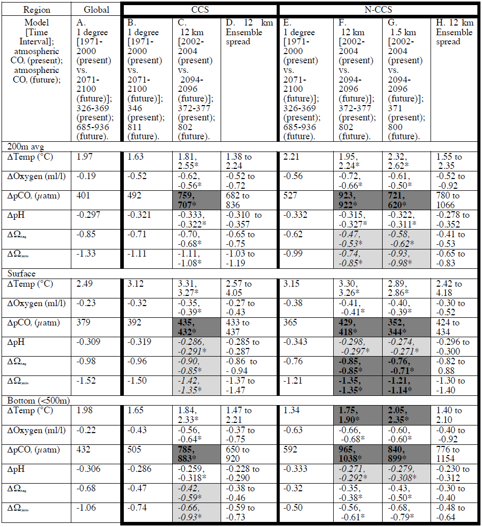
Table 1 Annual average differences between climate stressor variables in the future and the base/present conditions for the global ensemble and 12 and 1.5 km projections over different regions of the water column (200 m averaged, surface, and bottom <500 m). Column A depicts the global average from the ensemble average of CMIP5. Column B includes the global (1^∘) ensemble average difference for the CCS region followed by, in column C, the CCS-wide difference from the 12 km downscaled results. The final CCS column (column D) includes the ensemble spread as the range across the five-member model spread of the results for the 12 km model projections column for the CCS domain. The N-CCS region results span columns E–H in this table. The next three columns detail the differences in the Cascadia domain for the global ensemble average (column E) and the 12 km (column F) and 1.5 km downscaled projections (column G). The final column (column H) includes the ensemble spread as the range across the five-member model spread of the results for the 12 km model projections column for the Cascadia domain. The direction with which each variable described above was amplified/dampened relative to the global models outside the ensemble variability is highlighted using bold text and dark grey (amplified) and italic text with light grey (dampened) shading. Within the downscaled simulation, values are also provided just on the shelf (<200 m isobath) and denoted with an asterisk (*) next to the number.

The 1.5 km projection was forced using the open-ocean boundary conditions and atmospheric forcing from the 12 km regional simulation described above (Howard et al., 2020b). The boundary conditions included biogeochemical fields from the 12 km model. Because the ecosystem model (BEC) in the 12 km parent grid has more variables than the Cascadia simulation, some of the variables were merged. Specifically, the phytoplankton fields were added together, and the nutrients (ammonia and nitrate) were summed into one nitrogen field. To ensure no biogeochemical model drift between the nested 1.5 km simulation and the 12 km simulation, after 1 year of spin-up, a simulation of 2007 was compared against observations from the region (Fig. 2). The 1.5 km biogeochemical model skill was similar to the original model runs previously published (Davis et al., 2014; Giddings et al., 2014; Siedlecki et al., 2015) for 2007 (Fig. 2) without any significant drift in time. Temperature and salinity both experienced a significant bias in the upper 200 m in this configuration, unlike the previously published model runs (Fig. 2; temperature RMSE: 2.43; salinity RMSE: 0.627). As we are focused on differences between the present day and the future and we expect the bias to remain the same, we do not bias-correct the forcing here.

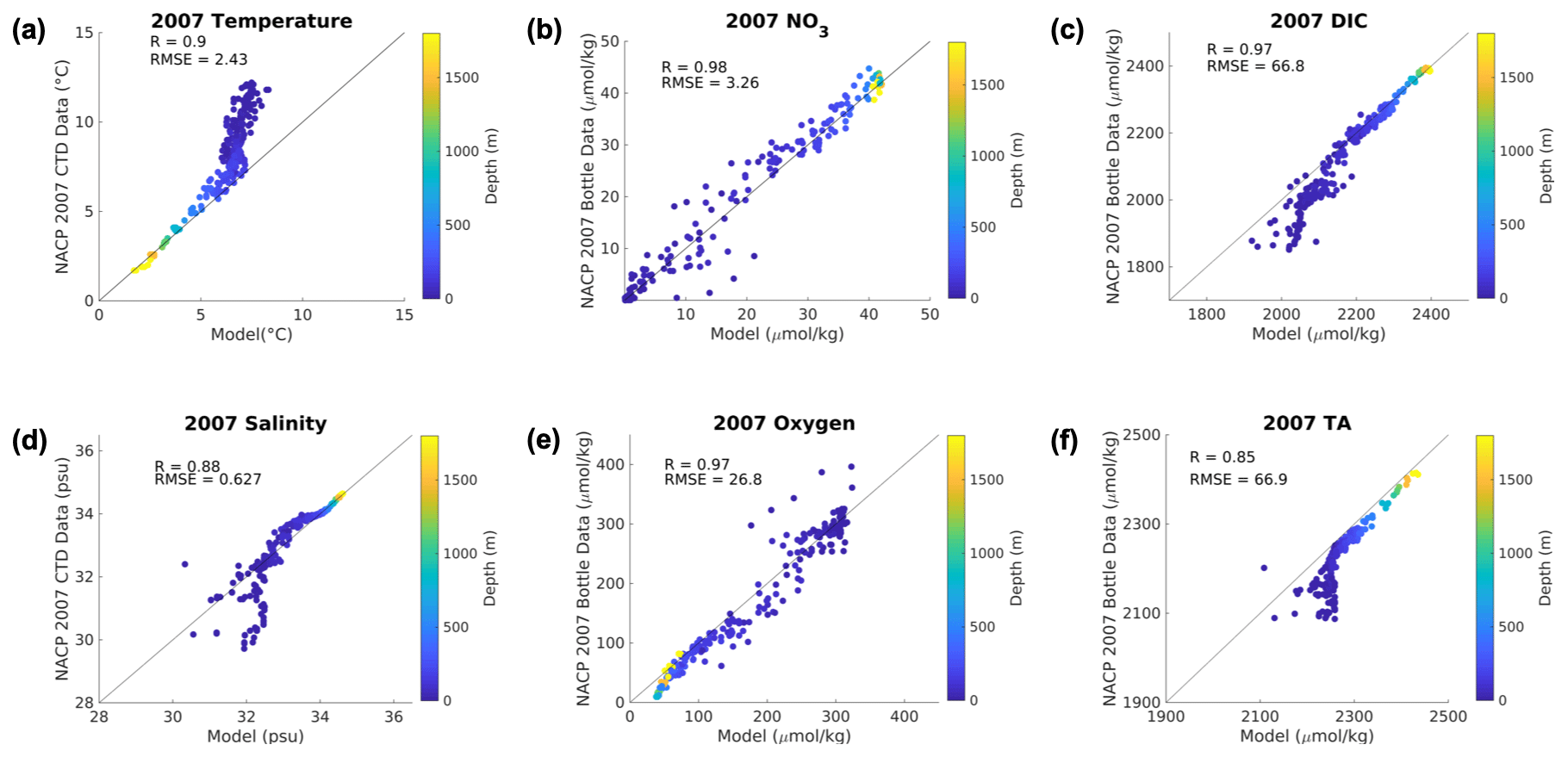
Figure 2 Model evaluation. Comparison between the bottle data from the 2007 cruise detailed in Feely et al. (2008) on the y axes and the simulated parameter (x axis) from the 1.5 km model forced with the 12 km model at the boundaries. Colors indicate the depth where the bottle sample was taken. Correlation coefficient (R) and root mean squared error (RMSE) are reported as well. The units for each variable are labeled on the axes.

For the future conditions, atmospheric CO₂ concentration (800 ppm) and future atmosphere and ocean forcing from the 12 km runs drove the Cascadia simulations. The river forcing was approximated by altering the timing of the freshet of the 2007 forcing earlier in the year by 2 months. This is in line with some historical analyses from the N-CCS region (Riche et al., 2014) as well as some projections of future hydrological conditions for the Fraser River (Morrison et al., 2002). Both of these results suggest that the total precipitation will remain the same, but the increase of rain and decrease in snowpack will shift the freshet earlier (Fig. S2 in the Supplement). The river TA was not altered from historical forcing, but the rivers equilibrate with the future atmospheric CO₂ concentration (800 ppm).

2.4 Future change

For each resolution, simulations were run for a number of years in a base/present state and then compared to a future simulation. The change is the difference between the future and base/present state, representing a ∼100-year anomaly due to climate forcing. The historical/base state for the CMIP5 runs was computed from an ensemble mean spanning 1971–2000. For the 12 km simulation, the base/present state spanned 1994–2007. For the 1.5 km simulation, the model was spun up for 1 year (2001), and then the base/present state spanned 2002–2004. Each level of resolution entails additional computer resource costs, which is part of the appeal of large-scale simulations. The CMIP5 future forcing used here spans a 30-year mean over 2071–2100. The 12 km model is a late-21st-century run spanning 2085–2100. The 1.5 km model is also a late-21st-century run spanning 2094–2096. Results and comparisons for the work presented using both the 12 and 1.5 km resolution simulations were made using the same year span despite runs existing for a broader range of years for the 12 km simulation. The present state was considered as 2002–2004 for both the 12 and 1.5 km simulations, and the future was 2094–2096 (Table 1). The global model ensemble average results represent a 30-year climatology.

2.5 Modification

The range of the five ensemble members which forced the 12 km projections is used to bound the potential futures expected. When the differences provided in Table 1 between the mean downscaled conditions for a region of the CCS (CCS-wide, columns B and C, or Cascadia/N-CCS, columns E–G) and the ensemble spread quantified from the 12 km model projections (columns D and H) both exceed the 1^∘ model projected change (columns B and E), those regions of the CCS are projected to undergo amplified change. The converse is referred to as dampening. The ensemble spread is provided in Table 1 as the range of the five-member model spread of the annual average results for the 12 km model projections (columns D and H). The direction with which each variable described above was amplified relative to the global models is highlighted using dark grey (amplified) and light grey (dampened) shading in Table 1.

3 Results

Model projections of climate-driven stressor variables (temperature, O₂, pH, saturation state (Ω), and CO₂) in each downscaled projection were compiled for the CCS for three depths (200 m averaged, surface, and bottom <500 m; Table 1; Figs. 3–5). The global average changes for many of these variables are different from the 1^∘ model projected values for the CCS region, but in only a few cases does this difference fall outside of the ensemble spread reported in column D and H of Table 1 (i.e., the signal is amplified or dampened). For each variable and depth, the change between the base state and the projected state is described below and evaluated within the context of the ensemble spread.

3.1 Temperature

The surface-to-200 m depth-averaged temperatures at all model resolutions are consistently warmer in the future CCS, both CCS-wide (1.63 and 1.81 ^∘C in the 1^∘ and 12 km models, respectively; columns B and C in Table 1) and within the N-CCS (1.95 to 2.32 ^∘C across the three model resolutions; Fig. 3a, columns E–G in Table 1). The Washington shelf experiences the largest projected differences in the 1.5 km projection (2.32 ^∘C, Fig. 3). The 1^∘ model projected increase for the CCS (1.63 ^∘C) and the N-CCS (2.21 ^∘C) falls within the range of warming from the downscaled projections (CCS: 1.38 to 2.24 ^∘C; N-CCS: 1.55 to 2.35 ^∘C, columns D and H in Table 1). In both regions of the CCS, the differences between the models are smaller than the range of the 12 km ensemble (Table 1).

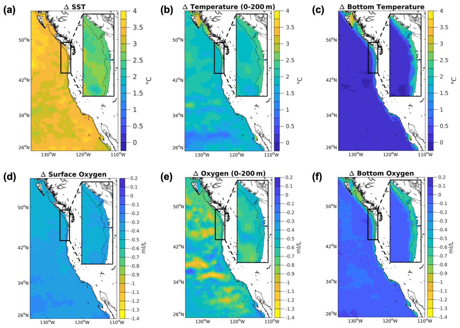
Figure 3 Projected temperature and oxygen changes in the CCS. Differences between climate stressor variables temperature and oxygen in the future and the base/present conditions for the 12 km (CCS-wide, full panel) and 1.5 km (N-CCS, inset) projections for (a) SST (^∘C), (b) depth-averaged temperature over the upper 200 m (^∘C), (c) bottom temperature (^∘C), (d) surface O₂ (mL L⁻¹), (e) depth-averaged O₂ over the upper 200 m (mL L⁻¹), and (f) bottom O₂ (mL L⁻¹). Positive values indicate a change that is greater in the future than the base/present condition, and negative values indicate lower values in the future than the base/present conditions depicted in Fig. 1.

At the surface, the SST is warmer in the future in all projections. Spatially, the SST increases most offshore, and increases least near the coast in all simulations of this eastern boundary upwelling system, as a result of upwelling (Fig. 3b). The 1.5 km model projects slightly smaller increases in SST than the 1^∘ model or the 12 km model. However, the 1^∘ models project SST increases CCS-wide (3.12 ^∘C) and in the N-CCS (3.15 ^∘C), which fall within the range of SST projections from the 12 km ensemble of downscaled projections (CCS: 2.57 to 4.05 ^∘C; N-CCS: 2.42 to 4.18 ^∘C; columns D and H in Table 1).

At the bottom, the temperature increases the most near the coast. The abyssal regions show little to no change in temperature (Fig. 3c). The shallowest regions of the 1.5 km simulation experience the largest warming – nearly 3 ^∘C. In the coastal-process-resolving downscaled projections, the projected bottom temperature change is greater (1.75–1.84 ^∘C, 2.05 ^∘C) than the global projections (1.34–1.65 ^∘C). However, the 1^∘ model projected increases for the whole CCS (1.65 ^∘C) fall within the range of temperature projections from the ensemble of 12 km projections (CCS: 1.47 to 2.21 ^∘C; column D in Table 1), while the N-CCS (1.34 ^∘C) is lower than the range of temperature projections from the ensemble of 12 km projections (N-CCS: 1.40 to 2.10 ^∘C; columns H in Table 1).

3.2 Oxygen

Annual depth-averaged O₂ concentrations at all model resolutions consistently decrease in the future compared with the base state, but the magnitude of the decrease is slightly more severe on average in the downscaled projections (Table 1; Fig. 3). The spatial variability within the CCS region, with more severe declines occurring in the N-CCS, is consistent across models but varies in magnitude. The 1^∘ model projected decrease for the CCS (−0.52 mL L⁻¹) and the N-CCS (−0.56 mL L⁻¹) falls within the range of the ensemble of projections from the 12 km model (Table 1; CCS: −0.52 to −0.72 mL L⁻¹; N-CCS: −0.52 to −0.92 mL L⁻¹; columns D and H in Table 1).

At the surface, O₂ declines in all projections, and the degree of change is similar across resolutions (Table 1; Fig. 3), consistent with the solubility effect from surface temperatures in each simulation. The 1^∘ model projected decline falls within the spread ensemble of projections from the 12 km model for the CCS.

The bottom O₂ concentration declines in all projections near the coast (Table 1; Fig. 3). The range of change in bottom O₂ on the shelf in the 1.5 km projection varies by a factor of 2, with the most extreme changes occurring on the outer shelf and in pockets known to experience persistent hypoxia in the present ocean – e.g., near Cape Elizabeth, south of Heceta Bank, and within the region associated with the Juan de Fuca Eddy (Siedlecki et al., 2015). The 1^∘ model projected decrease for the CCS (−0.43 mL L⁻¹) and the N-CCS (−0.63 mL L⁻¹) falls within the ensemble range of the ensemble of bottom O₂ concentration projections from the 12 km model (CCS: −0.37 to −0.75 mL L⁻¹; N-CCS: −0.40 to −0.92 mL L⁻¹; columns D and H in Table 1). When the bottom is restricted to the shelf in the downscaled simulations (<200 m isobath; values with asterisk (*) in Table 1), this decrease is more severe but still does not fall outside the range from the comparable depth range of the 1^∘ model projection (<500 m).

3.3  pCO₂

All model projections of pCO₂ consistently increase, with larger increases in the downscaled projections than in the global projection (Table 1; Fig. 4). The spatial variability within the CCS region differs across resolutions. All projections show an onshore–offshore gradient in pCO₂ with smaller changes closer to the coast and larger changes offshore. In the coastal-process-resolving downscaled projections, the projected depth-averaged change in pCO₂ increases, and the gradient between the nearshore and offshore intensifies. The 1^∘ model projected increase for the CCS (492 µatm) and the N-CCS (527 µatm) falls below the ensemble range of downscaled pCO₂ projections from the 12 km model (CCS: 682–836 µatm; N-CCS: 780 to 1066 µatm; columns D and H in Table 1).

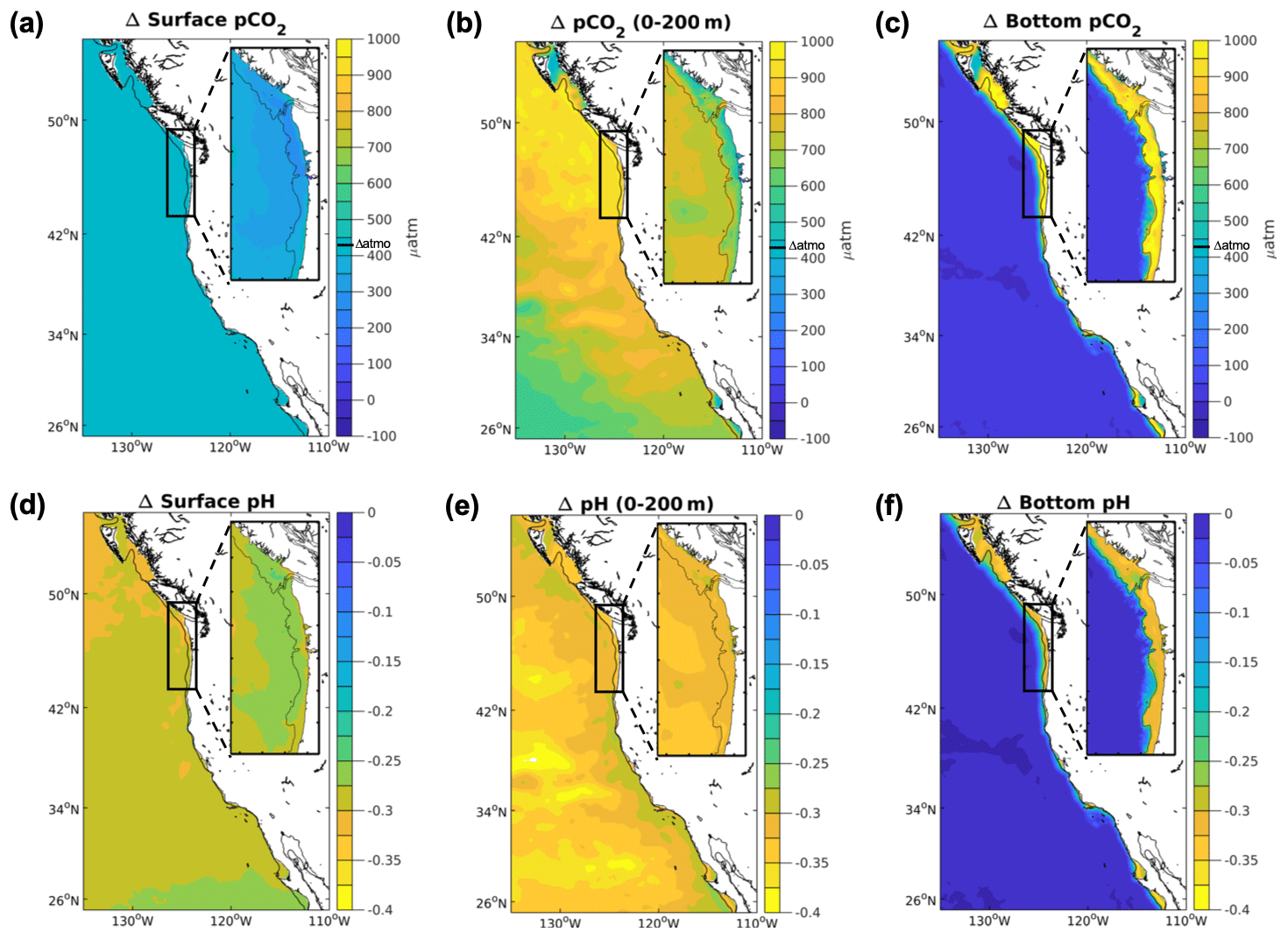
Figure 4 Projected pCO₂ and pH changes in the CCS. Differences between climate stressor variables pCO₂ and pH in the future and the base/present conditions for the 12 km (CCS-wide, full panel) and 1.5 km (N-CCS, inset) projections for (a) surface pCO₂ (µatm), (b) depth-averaged pCO₂ over the upper 200 m (µatm), (c) bottom pCO₂ (µatm), (d) surface pH, (e) depth-averaged pH over the upper 200 m, and (f) bottom pH. Positive values indicate a change that is greater in the future than the base/present condition, and negative values indicate lower values in the future than the base/present condition depicted in Fig. 1.

At the surface, future pCO₂ consistently increases in all projections but varies widely across resolutions (Table 1; Fig. 4). In the downscaled projections, most upwelling areas experience a smaller increase in surface pCO₂ than offshore waters. In the 1.5 km projection, regions near the coast of Oregon show the largest surface pCO₂ differences between the base and future states, while the region associated with the Columbia River plume shows a much smaller change. Overall, the inclusion of coastal processes contributes to the spatial patterns and magnitudes of projected changes. Consistent with the subsurface signal, the 1^∘ model projected increase for the CCS (392 µatm) and the N-CCS (365 µatm) falls below the ensemble range of the downscaled projections from the 12 km model (CCS: 433 to 437 µatm; N-CCS: 424 to 434 µatm).

At the bottom, pCO₂ is consistently higher in all projections, with varying magnitude across the model resolutions (Table 1; Fig. 4). The range of change in bottom pCO₂ on the shelf of the 1.5 km projection varies widely (600–1200 µatm), with the most extreme changes occurring on the outer shelf and in pockets known to experience persistent hypoxia at present. The 1^∘ model projected change for the CCS (505 µatm) and the N-CCS (592 µatm) falls below the ensemble range of projections from the 12 km downscaled model (CCS: 650 to 920 µatm; N-CCS: 776 to 1154 µatm).

3.4 pH

The pH averaged over 200 m depths for all model resolutions consistently decreases, and change is less severe than the global models project for the CCS region (Table 1; Fig. 4). In the 12 km simulation, a slightly smaller pH change (∼ −0.26) is observed in the southern CCS than the entire CCS, within the influence of coastal upwelling. In the 1.5 km simulation, the regions of largest decline are on the outer shelf and patches of the Oregon shelf. In the downscaled projections, the depth-averaged 200 m pH is lower than the 1^∘ model projected change in the north and greater than the global change CCS-wide. The 1^∘ model projected decrease for the CCS (−0.321) and the N-CCS (−0.332) falls within the ensemble range of projections for the downscaled 12 km model (CCS: −0.310 to −0.357; N-CCS: −0.278 to −0.352).

At the surface, the pH consistently decreases in all projections and is less severe a decrease in the downscaled projections than for the same region in the global model (Table 1; Fig. 4). The 1^∘ model projected decrease for the CCS (−0.319) and the N-CCS (−0.343) is larger than the ensemble range of projections for the downscaled 12 km model (CCS: −0.285 to −0.287; N-CCS: −0.296 to −0.300).

At the bottom, the pH decreases on the shelf in all projections (Table 1; Fig. 4). In the 1.5 km resolution model, the projected conditions show spatial variability on the shelf that is not apparent in the coarser models. The most severe changes in bottom pH correspond with regions that experience the largest changes in bottom O₂. The downscaled projections indicate decreases in annual average bottom (< 500 m) pH, but spatial variability exists on the shelves in the coastal-process-resolving simulations. This difference between the 1^∘ and downscaled simulations is even greater on the shelves (indicated as the starred values in Table 1). The 1^∘ model projected decline for the CCS (−0.286) falls within the ensemble range for the downscaled 12 km model (CCS: −0.228 to −0.290), while the N-CCS 1^∘ model projection (−0.333) is larger than the ensemble range of projections (N-CCS: −0.230 to −0.312) for the downscaled 12 km model.

3.5  Ω

Projections of Ω_arag and Ω_calcite averaged over 200 m depths at all model resolutions consistently decrease in the future, but the magnitude of decrease is usually greater in the downscaled projections (Table 1; Fig. 5). The projected difference is greater on the shelf than offshore, but this gradient is weaker in the 1.5 km projection. The 1^∘ model projected decline in Ω_arag for the CCS (−0.71) falls within the ensemble range of projections for the downscaled 12 km model for the CCS (−0.65 to −0.75). The 1^∘ projected decline in Ω_arag for the N-CCS (−0.62) is larger than the ensemble range of projections and larger than the ensemble range of projections for the N-CCS (−0.41 to −0.53) in the downscaled 12 km model. The same patterns are true for the Ω_calcite averaged over 200 m depths (Table 1).

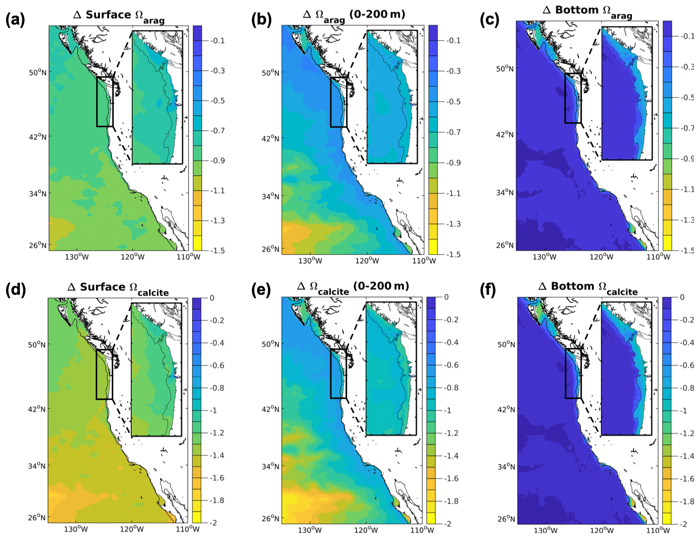
Figure 5 Projected Ω changes in the CCS. Differences between climate stressor variables Ω in the future and the base/present conditions for the 12 km (CCS-wide, full panel) and 1.5 km projections (N-CCS, inset). (a) Surface Ω_arag, (b) depth-averaged Ω_arag over the upper 200 m, (c) bottom Ω_arag, (d) surface Ω_calcite, (e) depth-averaged Ω_calcite over the upper 200 m, and (f) bottom Ω_calcite. Positive values indicate a change that is greater in the future than the base/present condition, and negative values indicate lower values in the future than the base/present condition depicted in Fig. 1.

At the surface, Ω consistently decreases in all projections (Table 1; Fig. 5). Spatially, the 12 km projection shows the largest declines in surface Ω in the southern domain, with little gradient between the shelf and offshore. At the 1.5 km resolution, the N-CCS projected declines are lowest offshore, and the declines are even larger than the 12 km projected changes even when considering the ensemble spread. The 1^∘ projected decrease for the CCS (−0.96) is larger than the range of the ensemble of projections from the downscaled 12 km model (CCS: −0.86 to −0.94). The 1^∘ projected decrease for the N-CCS (−0.76) is smaller or less severe than the range of the ensemble of projections from the downscaled 12 km model (N-CCS: −0.82 to −0.88). The same is true for the surface decline Ω_calcite (Table 1).

At the bottom, Ω decreases in all projections near the coast on the shelves (Table 1; Fig. 5). At the 1.5 km resolution, spatial variability in the magnitude of the projected conditions exists on the shelf. The most severe changes in bottom Ω correspond with regions that experience the largest changes in bottom O₂. In the N-CCS, the 1.5 km projected declines are even larger than the 12 km projected declines even when considering the ensemble range. The 1^∘ model projected decline in Ω_arag for the CCS (−0.47) is more severe than the downscaled ensemble range (CCS: −0.38 to −0.46) for the downscaled 12 km model. In the N-CCS, the 1^∘ model projected decline in Ω_arag for the N-CCS (−0.32) falls within the range of the ensemble of projections from the downscaled 12 km model (−0.30 to −0.40). In the 1.5 km model projections, the decline is greater than the 1^∘ model projects and falls well outside the range of the 12 km projections. This difference between the global and downscaled simulations is even greater on the shelves (indicated as the starred values in Table 1). The same is true for the bottom decline in Ω_calcite (Table 1).

3.6 Themes across projected changes for the CCS

All climate-associated stressor variables agree with the 1^∘ projections in terms of the direction of the trend, but not the magnitude of the change. The 1^∘ model projections for the CCS are largely consistent with the 1^∘ model projected global trends, with some differences in the nearshore upwelling areas (Fig. S1). All carbon variables are sensitive to the inclusion of coastal processes, which both downscaled projections provide. In addition, all of the projections suggest greater change in most variables in northern regions of the CCS and in the upwelling regions.

Nitrate increases over much of the domain in the upper 200 m (Fig. 6, Table S1 in the Supplement) in both the high- and medium-resolution downscaled simulations. Nitrate on average increases in the global simulations, but the magnitude and direction vary widely across the ensemble members, a result consistent with Howard et al. (2020b). In addition to the projected small increase in nutrient concentrations in the upwelling system of the CCS, the winds are slightly more intense (2 % increase in the magnitude of the wind stress) during the upwelling season (April–September) in the future years. The timing of the onset and duration of the upwelling season in the northern CCS remains the same in the future in these projections. Despite these differences from wind-based upwelling metrics, the in-water upwelling metric CUTI indicates no net change in the upwelling intensity of the future N-CCS in the simulations evaluated here. When nitrate is included in the upwelling measure, as in BEUTI, there is a slight decline in the upwelling of nitrate (1–2 %), consistent with a decrease in nitrate at the surface in the N-CCS (Fig. 6). This result is sensitive to the distance offshore (20–75 km) over which the index is calculated. The direction of the trend does not change, but BEUTI, for example, further declines (4 %) as bin boundaries move closer to shore. The further offshore the bin extends, the weaker the signal becomes. Both of these measures suggest that the upwelling is not intensified in our projected future, despite the slight increase in winds. This result is consistent with the results of Howard et al. (2020b), where increased stratification in the future simulations impeded increases in upwelling intensity.

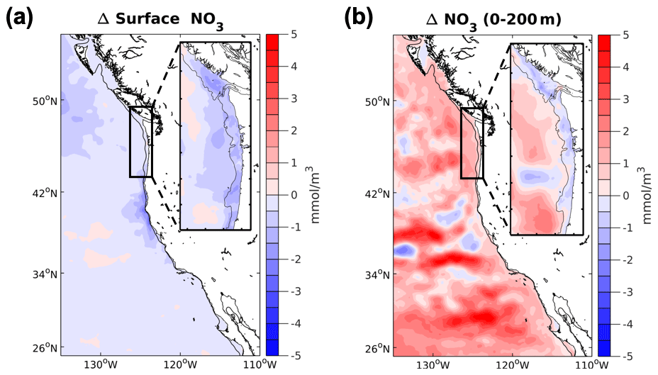
Figure 6 Projected changes in nitrate for the CCS. Differences between the future and the base/present nitrate (NO₃) conditions for the 12 km (CCS-wide, full panel) and 1.5 km (N-CCS, inset) projections (a) at the surface and (b) depth-averaged (0–200 m). Positive values indicate a change that is greater in the future than the base/present condition, and negative values indicate lower values in the future than the base/present condition.

The projected temperature change affects the solubility of the gases, generating a solubility-driven decline, and the increased nutrient content would correspond to a stoichiometric oxygen loss as well. Over the entire CCS, the decrease in oxygen over the upper 200 m was 0.45 mL L⁻¹ or 20.10 mmol m⁻³ (Table 1). The solubility-driven change accounts for most (∼67 %) of this change (13.42 mmol m⁻³ using 1.92 change in temperature from Table 1). The additional nitrate brought into the region from the large-scale models (0.79 mmol m⁻³) corresponds to an additional drawdown of 6.81 mmol m⁻³ of oxygen. In the N-CCS, the change in oxygen is a bit larger than across the entire CCS – 0.69 mL L⁻¹ (30.82 mmol m⁻³, Table 1). The solubility-driven changes contribute a bit less (∼44 %) in the N-CCS than the entire CCS, but the nitrate signal is larger in the N-CCS, corresponding to 11.21 mmol m⁻³ change in oxygen from an increase of 1.3 mmol m⁻³ of nitrate in the upper 200 m of the water column. The result is that the solubility-driven changes combined with the increased supply of nutrients to the upper 200 m of the N-CCS accounts for 80 % of the projected oxygen change in the N-CCS.

Similarly, we would expect carbon content to increase in source waters commensurate with an increase in nutrients and lower oxygen concentrations. The corresponding stoichiometric increase in DIC to the increase in nutrients (5 mmol m⁻³) would only account for a small decline in pH (0.02) or Ω (0.03). The majority of the pH and Ω decline is due to anthropogenic carbon content increase in DIC associated with the RCP8.5 scenario forcing (∼95 mmol m⁻³). Spatial variability in ΔDIC corresponds with variability in the water buffer capacity and Revelle factor, with southern CCS regions of relatively high buffer capacity having the greatest rates of DIC uptake (Fig. 7, Table S1).

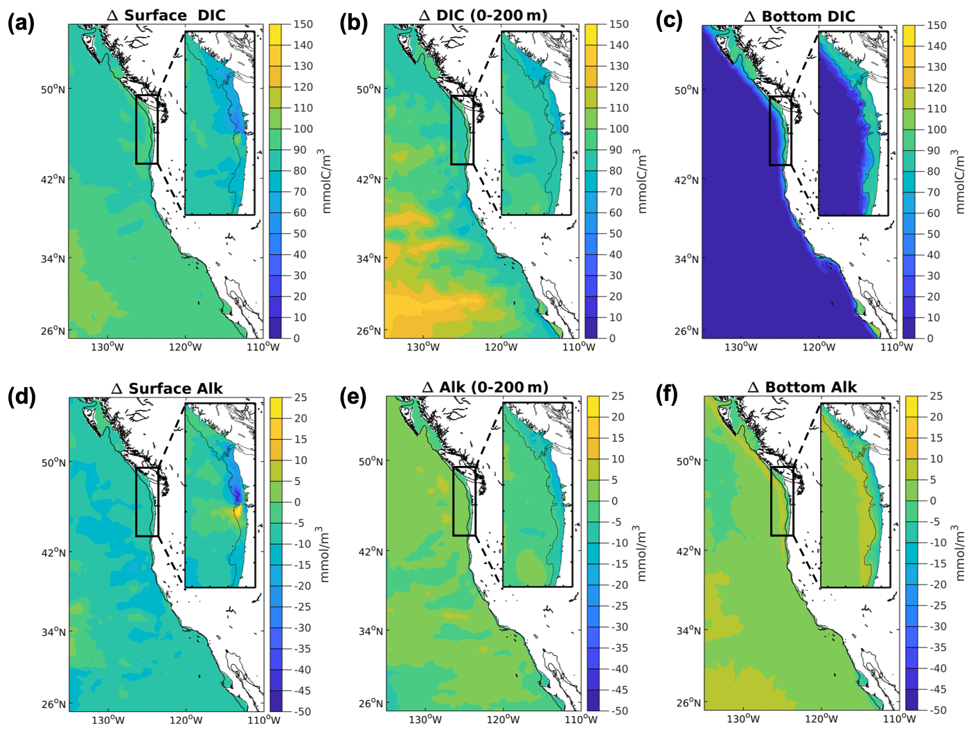
Figure 7 Projected changes for DIC and TA in the CCS. Simulated downscaled changes in annual average DIC and TA (mmol m⁻³) in the future and the base/present conditions for the 12 km (CCS-wide, full panel) and 1.5 km (N-CCS, inset) projections. (a) Surface DIC (b), 200 m depth-averaged DIC, (c) bottom DIC, (d) surface TA, (e) 200 m depth-averaged TA, and (f) bottom TA. Positive values indicate a change that is greater in the future than the base/present condition, and negative values indicate lower values in the future than the base/present condition.

TA increases in the future in the subsurface on the shelves of the CCS and even more so on the upper slope (Fig. 7, Table S1), but it mostly decreases across domains. At the surface, it declines, and these two changes offset each other in the depth-averaged 200 m change. Overall, the decrease in TA in the projections from the downscaled simulations is substantially smaller than the decrease from the 1^∘ models (Table S1). These changes in their corresponding depth ranges contribute to the results for the carbon variables in Table 1, impacting different carbon variables differently; for example, pCO₂ is amplified while pH is not modified over much of the CCS, and Ω is amplified at the bottom and the surface but dampened over the upper water column. These patterns will be examined more closely in Sect. 3.7, which focuses on modification and which follows.

On the shelves of the downscaled simulations, the source waters are further modified by coastal processes, including increased benthic–pelagic coupling, freshwater delivery, and denitrification. The inclusion of these processes causes the bottom waters on the shelf to experience a more severe increase in pCO₂ and declines in oxygen, pH, and Ω than observed in the shallowest regions of the global models (starred values in Table 1). The difference between the bottom estimated changes in the CCS in the depth ranges resolved by the global models and on the downscaled shelves is greatest for the carbon variables.

3.7 Modification

In general, the CCS experiences a greater change for most variables at all resolutions than the global ocean. However, only the carbon variables emerge as amplified or dampened by the downscaled simulations. Across the spread of ensemble members for the entire CCS in the 12 km simulation, the downscaled projected increase for pCO₂ (columns C, F, and G) is amplified relative to the 1^∘ models (columns B and E) in all three depth ranges (Table 1). The N-CCS pCO₂ increase is amplified in both downscaled simulations (12 and 1.5 km) at all depth ranges (Table 1, columns F and G). In the 200 m depth-averaged changes, the pCO₂ change is correlated to the TA changes (Table S2). The changes in pCO₂ are correlated to the temperature at the surface and to DIC, TA, and nutrient changes at the bottom (Table S2).

The downscaled decrease in pH at the surface and the bottom is modified relative to what the 1^∘ models project for the CCS and N-CCS in the downscaled projections. The surface change is less severe than in the 1^∘ model and so is considered dampened relative to global change. At the bottom, pH in the N-CCS is dampened relative to the 1^∘ model. In both downscaled projections (12 and 1.5 km), the surface and bottom pH decrease is dampened in the N-CCS relative to the surface pH decline in the 1^∘ model for that region (column E). While pH is not modified in the 200 m depth-averaged changes, at the surface the pH changes are correlated to the DIC and TA changes (Table S2).

The decrease in Ω over the upper 200 m is less severe than the 1^∘ model projection for the N-CCS and falls outside of the ensemble range, so it is considered dampened relative to global change (Table 1). The N-CCS 200 m depth-averaged Ω decrease is dampened in both downscaled simulations (12 and 1.5 km) and amplified at the surface (Table 1). At the surface, the changes in saturation state are highly correlated to DIC changes. At the bottom, the changes are also correlated to the changes in nutrients (Table S2). In the N-CCS region, more of the water column is modified for the carbon variables.

4 Discussion

Globally, under RCP8.5, the future oceans simulated using CMIP5 are projected on average to be warmer (SST, mean±1SD: 2.73±0.72 ^∘C), higher in pCO₂, lower in O₂ content (RCP8.5: $-\mathrm{3.45}\pm \mathrm{0.44}$ %), and more acidified (surface pH: $-\mathrm{0.33}\pm \mathrm{0.003}$ units) (Gattuso et al., 2015). Regionally, the CMIP5 models project the North Pacific to be one of the regions to experience the most warming, most severe O₂ declines, and largest extents of corrosive conditions (Bopp et al., 2013; Feely et al., 2009; Gattuso et al., 2015; Gruber et al., 2012; Hauri et al., 2013; Long et al., 2016). Here, we present one of the first downscaled multivariable projections of environmental change out to the end of the century in the CCS driven by a suite of CMIP5 forcings instead of a single global model. While the downscaled projections show changes that are similar in direction to those of the global simulation, the magnitude and spatial variability of the change differ in the coastal-process-resolving downscaled projections and to a varying degree depending on the variable, depth range, and subregion of interest.

The CCS experiences a greater change for many variables at all resolutions than the global ocean; however this change is modified in the CCS in both downscaled simulations (12 and 1.5 km) for pCO₂, Ω_arag and Ω_calcite, and pH. Amplification of global trends within the CCS upwelling systems in the future has been shown before for oxygen specifically (Dussin et al., 2019) and was identified through the response of the downscaled model to a series of idealized experiments with perturbations in the source water oxygen and nutrient concentrations. Source water changes in oxygen drove a 2-fold-larger change in oxygen than nutrient supply alone, and both of these drivers were determined to be more important than intensifying winds. In our projections, the more realistic winds were different than in Dussin et al. (2019), with a small intensification of about 2 %. The source waters were lower, but the oxygen decrease in the N-CCS fell within the range of the ensemble members explored here. Dussin et al. (2019) only explored one global model (GFDL) as a driver, and as such the definition of amplification differs from the one we use here. Much like experiments conducted by Liu et al. (2012, 2015) for ocean temperatures and described in Alexander et al. (2020), using a multi-model mean to drive a downscaled ocean model retains the linear component of the climate change forcing only and is not able to assess the range of the response. Fundamentally, our definition of amplification relies on the range of the ocean condition responses. The mechanism of remote biogeochemical redistribution and influence via boundary conditions in the CCS remains influential for the carbon variables that were identified as amplified here. While climate stressor variables have been identified as amplified historically using records spanning several decades or more (Chavez et al., 2017; Osbourne et al., 2020), regional future projections have focused on multi-model mean conditions projected over 100 years into the future.

Although the downscaled model projected a small intensification in the projected upwelling-favorable wind stress of 2 %, which is consistent with prior work on this topic (Bakun, 1990; Garcia-Reyes et al., 2015; Rykaczewski and Dunne, 2010; Rykaczewski et al., 2015), no change was quantified in the upwelling fluxes in the water column using the CUTI, and a slight decline was observed in BEUTI (nutrient flux) measures of upwelling. This is likely due to the compensation from increasing stratification in the future simulations as noted in Howard et al. (2020b). We observe lower oxygen and higher nutrient content in source waters, but this change does not make it to the surface. Within the CCS, solubility-driven oxygen changes are important, which is consistent with oxygen escape from the ocean being increasingly important in future projections (Li et al., 2020). Moving south within the CCS, solubility increasingly outcompetes nutrient-driven changes in oxygen drawdown. However, the projections here indicate that the magnitude of oxygen decrease was within the bounds of the ensemble range and so was not amplified relative to the global models, unlike the carbon variables.

The projected change in pH is consistent with prior pH projections for the CCS downscaled with the same RCP8.5 scenario using a ROMS model (Gruber et al., 2012; Hauri et al., 2013; Marshall et al., 2017; Turi et al., 2018). These projections were performed with different biogeochemical models described in Gruber et al. (2012) and Fennel et al. (2006, 2008) and relied on multi-model means or individual ensemble members for the global models. The pH values we obtained are lower than the projections of Rykaczewski and Dunne (2010) for the CCS. They used GFDL Earth System Model 2.1, a different forcing scenario, and a different biogeochemistry model (Dunne et al., 2007). Despite clear modification of global trends indicated by downscaled projections provided here of pCO₂, Ω, and pH, the biogeochemical model formulations differ across resolutions and may be contributing to the amplified signals. Differences include parameterizations of gas exchange, detritus classes, sinking velocities, and benthic boundary conditions; the latter has been identified in prior work to be important for O₂ models in coastal regions (Moriarty et al., 2018; Siedlecki et al., 2015). Any of these could contribute to the differences observed across model resolutions. CMIP5 results are based on an ensemble average of many models, which all utilize different formulations and complexities for their ecosystem models, further contributing to the uncertainty provided from the biogeochemical boundary conditions. Overall, the projected annual depth-averaged change in pH appears to depend mostly on the anthropogenic forcing scenario, and all the models agree on the direction and relative magnitude despite these differences.

Projected changes in surface and bottom pH, Ω, and pCO₂ are modified by the inclusion of coastal processes when downscaling is employed. The variability of carbon variables is influenced by coastal processes in these regions of the water column. Those processes include the delivery of freshwater and sediment–water interactions. At the surface, pH, Ω, and pCO₂ change differently. TA declines at the surface, while DIC increases. DIC increases due to increased storage of carbon from the increase in carbon in the future atmosphere. The TA changes are driven in part by the altered timing of the freshet in the N-CCS as well as the presence of a river plume in an upwelling regime. Freshwater in the region is known to be corrosive due to naturally low TA, which impacts the buffering capacity of the surface waters. This result can be seen in the surface difference plots for pCO₂ near the Columbia River plume (Fig. 4) and the surface TA change (Fig. 7). The 12 km projections include climatological freshwater fluxes as precipitation along the coastline instead of resolving river plumes like the 1.5 km projections, but, despite these different freshwater parameterizations, both models indicate modification of carbon variables in the N-CCS Cascadia domain with different directions for different variables. While the freshwater amplifies the global rate of change for the surface pCO₂ and Ω, over the entire water column (200 m average), the pH change is dampened as the DIC and TA changes are offset by the temperature changes for that variable.

In our regional downscaled simulations, the changes in temperature and TA act together to offset the increase in the DIC signal in the coastal upwelling regime (Fig. 7), and for pH these changes offset each other in the upper 200 m of the water column. The global models show very little change in TA in the region. While the downscaled bottom TA change is small (20–50 mmol m⁻³, Fig. 7, Table S1), this amounts to an increase in pH of 0.07–0.18 and an increase in Ω of 0.15–0.21 – enough to offset 40–60 % of the reduction in Ω due to increased atmospheric CO₂ concentrations. At the bottom, the increase in TA modifies the projected pH change in the N-CCS by reducing it.

Both biogeochemical models include denitrification at the sediment water interface, which impacts both the nitrogen and TA cycling in the model. Denitrification is a source of TA (Chen, 2002) and has been shown to impact shelf-wide TA in other regions (Fennel et al., 2008). In the CCS, denitrification has been observed on the shelf and slope, peaks on the slope, and is greater off the Washington coast than off Mexico (Hartnett and Devol, 2003). As the source waters become lower in oxygen content, denitrification should increase, providing an additional feedback on the nutrients and carbon variables and dampening the global ocean acidification signal. Bottom Ω is not amplified in Table 1, but if calculated solely over the shelf region (asterisks in Table 1), then bottom Ω changes are amplified in both domains. While this source of alkalinity has not been observed directly in the present-day ocean, a source of TA was identified and interpreted as calcium carbonate dissolution in the CCS (Fassbender et al., 2011). These results suggest future projections should consider salinity and TA forcing feedbacks when performing regional projections as these can alter regional impacts of carbon variables.

Different carbon variables are sensitive to different physical climate forcings, a result that is consistent with recent work suggesting that competing sensitivities may dampen the variability of pH in the future (Jiang et al., 2019; Kwiatkowski and Orr, 2018; Salisbury and Jonsson, 2018; Takahashi et al., 2014). The sensitivities of the various carbon variables to thermal and geochemical (carbon dioxide) forcing were explored in an idealized simulation of future conditions from CMIP5 models in Kwiatkowski and Orr (2018), in the present-day ocean in Takahashi et al. (2014) and Jiang et al. (2019), and in the Gulf of Maine by Salisbury and Jonsson (2018). Kwiatkowski and Orr (2018) determined that the balance between the change in DIC and TA drives the variability of pH, in combination with temperature in mid-to-high latitudes – effects that largely cancel each other out. While the processes that control TA and DIC are similar, the addition of atmospheric CO₂ changes DIC alone, altering the balance between these two reservoirs. In the Gulf of Maine, temperature and salinity anomalies in combination with TA variability offset the long-term ocean acidification trend (Salisbury and Jonsson, 2018). Their analysis indicated that Ω is more sensitive to temperature and salinity variations than pH, and this result was confirmed globally in Jiang et al. (2019). Kwiatkowski and Orr (2018) also found the seasonal amplitude of Ω_arag is expected to strengthen in some regions and attenuate in others due to the high sensitivity of this variable to temperature.

By examining the relationships between the carbon variables and other regional variables, the relative importance of different processes responsible for the modification of carbon variables by coastal systems can be inferred. Themes emerge in the correlations with carbon variables across different regions of the water column: at the surface, DIC changes are important; at the bottom, changes in DIC, TA, and nutrient content changes have the highest correlations with more than one carbon variable. Over the 200 m water column, TA is important. The TA decreases in all the projections but by an order of magnitude less than the 1^∘ models in the downscaled simulations (Table S1). A dampened reduction in TA is consistent with changes in the biological metabolism or benthic–pelagic coupling alongside the sedimentary processes in the region – all of which can act as a source of TA on shelves.

If we take a specific example of Ω, the Ω changes are correlated with nutrient content changes, in addition to the DIC changes that result from the emissions scenario forcing. As a result, bottom Ω on the shelf is modified by the TA generation organic matter remineralization and via sedimentary processes. Consistent with this result, the bottom change in DIC is greater in the downscaled simulations than the 1^∘ models (Table S1). The 1^∘ models do not resolve the shelf bathymetry or, consequently, the sedimentary processes that seem likely to play an important role in this coastal setting.

These results are consistent with the idea that the changes in different regions of the water column are driven by different mechanisms – surface changes in the carbon variables are driven by the RCP and modified by coastal biological cycles, bottom conditions are influenced more by benthic–pelagic coupling and sedimentary processing as suggested by the TA and nutrients correlations, and the water column modification is a combination of all of these.

Spatially, within the CCS, the projections suggest greater change in most variables in northern regions of the CCS and on the shelves in the annual averages. Currently, the N-CCS is the most productive region of the CCS (Davis et al., 2014; Hickey and Banas, 2008) and experiences the most prevalent hypoxia (Connolly et al., 2010; Peterson et al., 2013) and corrosive events (Feely et al., 2018, 2016). One aspect that differentiates the region from the rest of the CCS is that the N-CCS experiences both seasonal upwelling and downwelling currently (Hickey and Banas, 2008), which is not projected to change in 2100 under RCP8.5. During the summer upwelling season in the N-CCS, oxygen declines on the shelf over the season as organic material and respiration increase on the shelf. Coincident with the oxygen decline, carbon parameters are impacted in kind (e.g., pH and Ω decreases and pCO₂ increases; Siedlecki et al., 2016; Feely et al., 2018). The dramatic fall transition on the Washington and Oregon shelves is observed in the present-day ocean (Adams et al., 2013; Connolly et al., 2010; Hales et al., 2006; Siedlecki et al., 2015), fully quantified by an oxygen budget in Siedlecki et al. (2015), and is projected to continue in the future projections examined here. The continued existence of a downwelling season in the future impacts some variables more than others. The projected change for oxygen and carbon variables is different seasonally. The fall transition and winter mixing re-oxygenates shelf waters (Siedlecki et al., 2015), and this pattern continues into the future. Hypoxia will continue to exist in the summer months, but for a longer period of the summer. Corrosive, low-pH conditions, however, will occur year-round. The fraction of the year during which bottom water on the shelf is corrosive (Ω<1) or low in pH (pH<7.65) nearly doubles. This asymmetry has been identified previously in the Salish Sea (Ianson et al., 2016) and exists because of the difference in equilibration timescales at the surface for oxygen and carbon dioxide.

5 Conclusions

We present one of the first multi-model, downscaled multivariable projections of changing temperature, pH, pCO₂, Ω, and O₂ in the CCS. The downscaled projections are driven by the same delta forcing as the global simulation, and projected changes for the CCS are consistent with the directional trends indicated by the global model for scenario RCP8.5 – warmer, more acidified, higher carbon content, and lower oxygen concentration. However, the magnitude and spatial variability of the change differ in the coastal-process-resolving downscaled projections and to a varying degree depending on the variable of interest. Changes in pCO₂ concentrations, Ω, and pH are modified in the downscaled projections relative to the projected global simulation, suggesting downscaled projections are necessary to more accurately project future conditions of these variables. Carbon variables are likely modified by the inclusion of shelf processes including benthic–pelagic coupling and sedimentary processing as suggested by the TA and nutrients correlations. The diversity of these projected changes of future ocean conditions emphasizes the need to improve our understanding of mechanisms by which coastal processes interact with these large-scale drivers of change or properly simulate and capture these feedbacks in projections.