the Creative Commons Attribution 4.0 License.
the Creative Commons Attribution 4.0 License.
 | 20 May 2021
Carbon export and fate beneath a dynamic upwelled filament off the California coast
Hannah L. Bourne
Elizabeth J. Connors
Todd J. Wood
To understand the vertical variations in carbon fluxes in biologically productive waters, four autonomous carbon flux explorers (CFEs), ship-lowered CTD-interfaced particle-sensitive transmissometer and scattering sensors, and surface-drogued sediment traps were deployed in a filament of offshore flowing, recently upwelled water, during the June 2017 California Current Ecosystem – Long Term Ecological Research process study. The Lagrangian CFEs operating at depths from 100–500 m yielded carbon flux and its partitioning with size from 30 µm–1 cm at three intensive study locations within the filament and in waters outside the filament. Size analysis codes intended to enable long-term CFE operations independent of ships are described. Different particle classes (anchovy pellets, copepod pellets, and > 1000 µm aggregates) dominated the 100–150 m fluxes during successive stages of the filament evolution as it progressed offshore. Fluxes were very high at all locations in the filament; below 150 m, flux was invariant or increased with depth at the two locations closer to the coast. Martin curve b factors (± denotes 95 % confidence intervals) for total particulate carbon flux were +0.37 ± 0.59, +0.85 ± 0.31, −0.24 ± 0.68, and −0.45 ± 0.70 at the three successively occupied locations within the plume, and in transitional waters. Interestingly, the flux profiles for all particles < 400 µm were a much closer fit to the canonical Martin profile (b−0.86); however, most (typically > 90 %) of the particle flux was carried by > 1000 µm sized aggregates which increased with depth. Mechanisms to explain the factor of 3 flux increase between 150 and 500 m at the mid-plume location are investigated.
- Article
(17168 KB) - Full-text XML
-
Supplement
(61 KB) - BibTeX
- EndNote


Carbon export driven by the biological carbon pump, the process by which photosynthetically derived biomass is transported out of the surface layer, is an important component of the global carbon cycle. Atmospheric carbon concentrations are in part controlled by the depth at which sinking organic matter is remineralized (Kwon et al., 2009) yet the fate of carbon exported to deeper waters beneath highly productive coastal regions is poorly understood. Current estimates for global carbon export range from 5 to > 12 Pg C yr−1 (Boyd and Trull, 2007; Henson et al., 2011; Li and Cassar, 2016; Dunne et al., 2005; Siegel et al., 2014, 2016; Yao and Schlitzer, 2013). Because coastal upwelling regions are such productive and unique ecosystems with complex current interactions, a question to be asked is as follows: is export of material to depth in these systems different than in open-ocean environments?. If so, knowing the rules governing particulate carbon export and remineralization in these regions will significantly advance carbon cycle simulations of CO2 uptake by the oceans.
While ocean colour satellites provide the temporal and spatial scale of phytoplankton biomass when clouds permit, flux beneath the euphotic zone is much more difficult to observe and therefore not as well known. A number of recent studies have noted discrepancies in reconciling meso- and bathypelagic activity with current euphotic zone flux estimates (Banse, 2013; Burd et al., 2010; Ebersbach et al., 2011; Passow and Carlson, 2012; Stanley et al., 2012). Measurements of new production (NP; Eppley and Peterson, 1979) should balance particle export measured at the same time if gravitational particle sinking dominates export; however, NP often is higher than particle export (Bacon et al., 1996; Estapa et al., 2015; Stukel et al., 2015). Mechanistic understanding of these differences is thus important to food web models.
The strength and efficiency of the biological carbon pump are governed by complex interactions between phytoplankton, zooplankton, and physical mixing. The Martin curve (Eq. 1), an empirical relationship, was derived from surface-tethered sediment trap observations made in the North Pacific during the VERTEX programme (Martin et al., 1987),
where F is flux at depth z, Fref is the flux measured at a reference depth zref (usually near the base of the euphotic zone), and b is a constant. Martin et al. (1987) found the best fits with . The choice of zref does not influence the derived b value.
Bishop (1989) compared the Martin and six other formulations for particle flux at depth in the open ocean and found that the Martin curve for predicting flux was most robust; while many profiles were fit with the classic Martin b factor of −0.86, the study found (in rare cases) b values of −0.3 to −1.5. Subsequent studies in the open ocean have yielded similarly varying b values, and all show the expected flux decrease with depth (Fig. 1) (Buesseler et al., 2007; Lutz et al., 2007; Marsay et al., 2015).
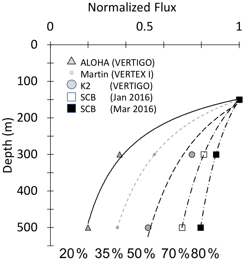
Figure 1Martin curves normalized to 150 m. Representative data from Martin et al. (1987), Buesseler et al. (2007), and Bishop et al. (2016). b values of lines from left to right are −1.33 (Stn. ALOHA), −0.86 (VERTEX I), −0.51 (Stn. K2), −0.19, and −0.3 (March and January 2016, Santa Cruz Basin). Transport efficiencies between 150 and 500 m range from 20 % (ALOHA) to 80 % (Santa Cruz Basin).
If all material sinking to depth is assumed to be gravitationally exported material originating from a stable photosynthetically derived source in the euphotic zone, an increase in material with depth should not occur. However, flux profiles that do not decrease monotonically with depth as predicted by Martin's formula have been observed, especially in regions that are both physically and biologically dynamic (e.g. Bishop et al., 2016, in the Santa Cruz Basin; Giering et al., 2017, in the North Atlantic), suggesting additional mechanisms contributing to particle flux are at play.
The California Current, the eastern boundary current of the North Pacific gyre, flows south from the sub-arctic North Pacific. Beneath it, the subsurface California Undercurrent flows poleward at depths between 200 and 500 m, with strong seasonal variability (Lynn and Simpson, 1987). Along the coast, the complex interactions of filaments, geostrophic flow, wind-driven Ekman transport, and mesoscale eddies distribute coastal waters. This leads to a heterogeneous pattern of productivity in surface waters with some regions (often in the vicinity of headlands) having very high productivity near centres of coastal upwelling, while others have intermediate productivity spurred by wind stress curl upwelling and other low-productivity regimes which reflect the onshore flow of oligotrophic waters (Gruber et al., 2011; Ohman et al., 2013; Siegelman-Charbit et al., 2018). In the summer, winds blowing south along the California coast cause surface waters to divert to the west, which allows deep nutrient-rich cold water to come to the surface. This water coming to the surface moves offshore in filaments which can extend offshore several hundred kilometres.
The California Current Ecosystem Long-Term Ecological Research (CCE-LTER) process study (1 June–2 July 2017; P1706) gave us the opportunity to observe carbon flux profiles beneath a rapidly evolving surface filament over its lifetime and to understand the magnitude, scales, and mechanisms of coastal production and its transport. During the study, we deployed carbon flux explorers (CFEs; Bishop et al., 2016, and Bourne et al., 2019) to depths of 500 m to observe particle flux variability and specifics of particle classes contributing to flux. Figure 2 shows the locations of CFE deployments and other activities during the CCE-LTER study, the Santa Cruz Basin (SCB) study site of Bishop et al. (2016), and the coastal station VERTEX 1 (Martin et al., 1987). The CCE-LTER study combined spatial surveys, three cross-filament CTD transects, and four sequentially numbered multi-day quasi-Lagrangian intensive sampling “cycles” within and outside of the filament. Cycles 1 to 4 correspond to locations 1 to 4 which are referred to as L1 to L4 below. L1, L2, and L4 represent sampling during the early, intermediate, and late stages of filament evolution. The order of occupations of L3 (outside of the filament) and L4 enabled a more complete view of filament evolution.
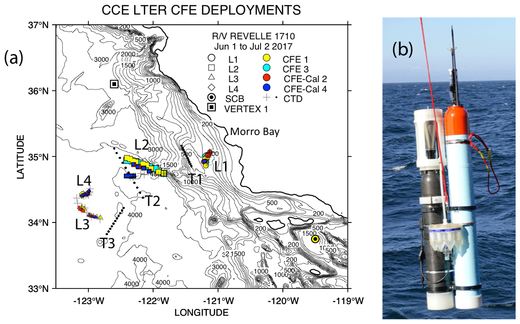
Figure 2(a) CFE and CTD deployments at locations L1 to L4. The CTD stations were close to a drifting surface-drogued productivity array. For the majority of stations, the CTDs and CFEs were close to one another. However, at L2, the CFEs diverged to the west-northwest of the drogued drifters. Dots depict locations of cross-filament CTD particle–optics transects T1, T2, and T3. T1 preceded work at L1; T2 was occupied after completion of sampling at L2. T3 was completed after work at L4. Data from transects shown in Fig. 11. (b) CFE-Cal during recovery.
In this study, we report autonomously measured carbon flux profiles in the mesopelagic zone beneath a filament of upwelled water off the coast of California and the finding at two locations (L1 and L2) that flux was invariant or increasing with depth, while flux decreased more slowly than predicted by the Martin formula at two other locations. We explore mechanisms for these flux profile observations. In the following discussion, we use the term “non-classic” to represent strong departures from the classic () Martin curve.
Study area
The June 2017 CCE-LTER process study aboard R/V Revelle followed a strong filament of upwelled cold, high-salinity westward-flowing water off the coast of California. In late May, cold water upwelled along the coast due to the intensification of upwelling-favourable north to south winds; shortly thereafter a filament developed near Morro Bay (35∘22′ N, 122∘52′ W, Fig. 2) and began propagating westward (Fig. 3a, b). Eventually, the filament extended 250 km offshore (Fig. 3c, d). By mid-June, the westernmost filament waters began to slow and developed into a cyclonic eddy which became pronounced in maps of sea surface height by the end of June (Fig. 4); locations L1–L4 are depicted in the maps.
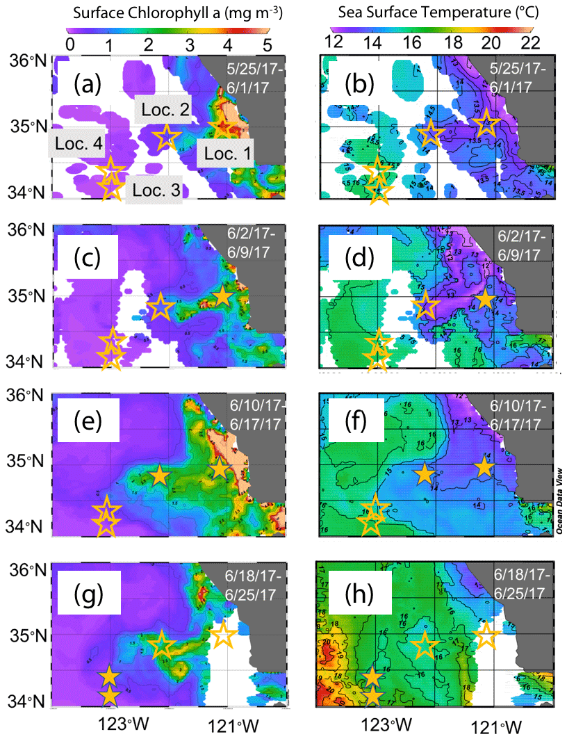
Figure 3Remotely sensed surface chlorophyll (a, c, e, g) and sea surface temperature (SST) (b, d, f, h) maps of the study area from late May to the end of June 2017. All images are from 4 km resolution, 8 d averaged data from VIIRS on the Suomi NPP satellite. The stars represent locations 1 to 4 where CFEs were deployed. Stars are filled in the panels most closely corresponding to the time of observations.
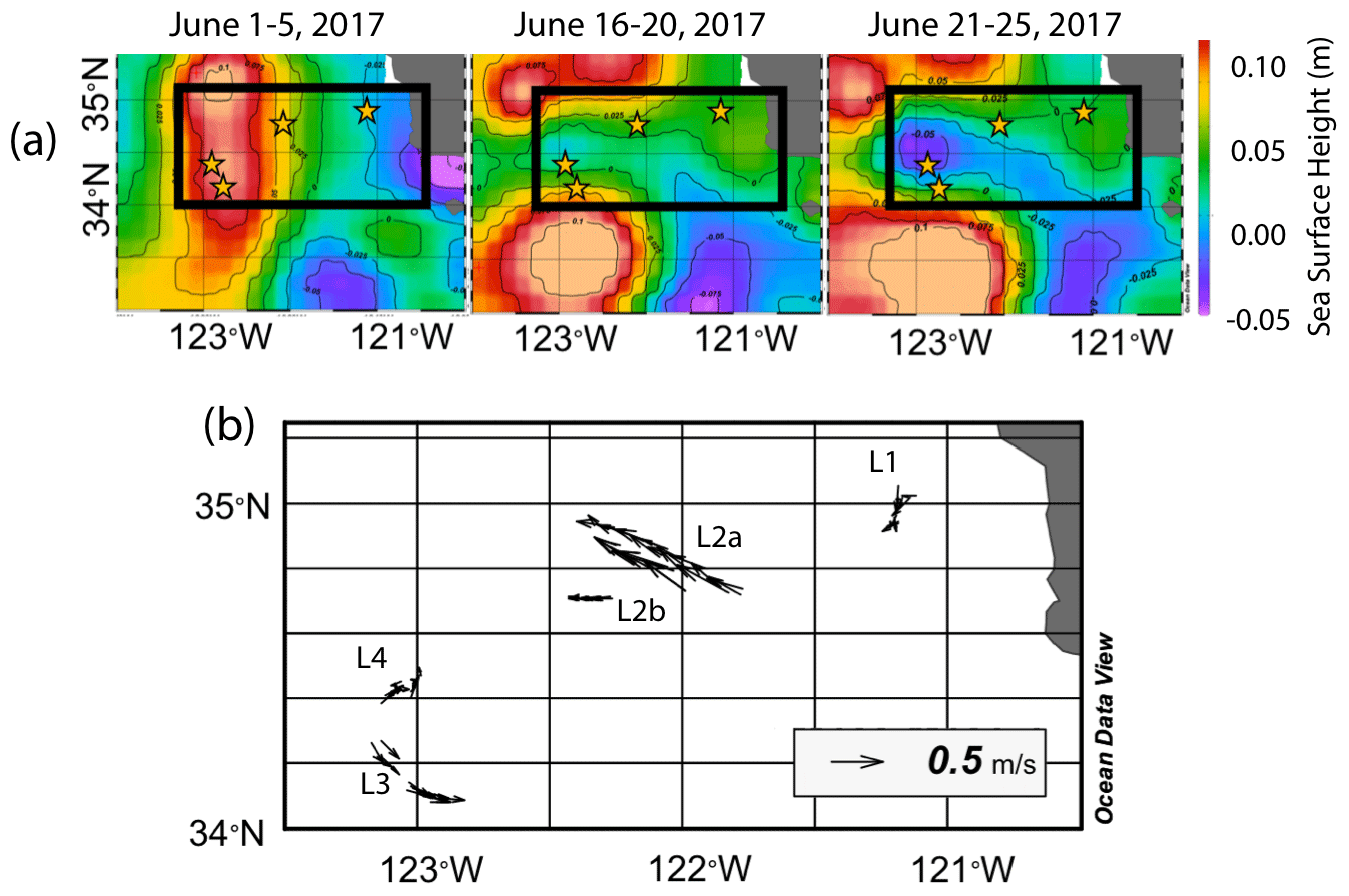
Figure 4(a) Average sea surface height from 1–5, 16–20, and 21–25 June 2017. In the beginning of June, sea surface height was low near the shore due to Ekman transport and higher off the coast. As the filament developed and moved to the west, a sea surface trough formed extending 200 km offshore and was first apparent in the 16–20 June map; it deepens in the 21–25 June map, indicating the formation of a cyclonic eddy. Anti-cyclonic eddies are present to the north and south. Stars represent positions of each location. (b) Velocity vectors for all CFE dives to depths of 500 m. The CFE motions were fastest at locations L2 and L3, where the CFEs were deployed near the edges of the cyclonic eddies and slowest at L1 inshore and at L4 which was located near the centre of the cyclonic eddy.
2.1 Remote sensing data
Satellite retrievals of sea surface temperature (SST), sea surface chlorophyll, and euphotic zone depth at 4 km spatial resolution and averaged at 1 or 8 d temporal resolution from SNPP VIIRS (Visible Infrared Imaging Radiometer Suite) and MODIS Aqua spacecraft were obtained from the NASA ocean colour archive (https://oceancolor.gsfc.nasa.gov/l3/, last access: August 2018). We similarly obtained Coastal Zone Colour Scanner (CZCS) data to provide context for the June 1984 Martin et al. (1987) VERTEX 1 station. Sea surface height (SSH) data (derived from a suite of spacecraft) were downloaded from the NASA Jet Propulsion Laboratory at ∘ and 5 d resolution (https://podaac.jpl.nasa.gov/, last access: August 2018; https://doi.org/10.5067/SLREF-CDRV1). Imagery was used in Figs. 3 and 4 to provide large-scale context for the study. Daily imagery was used to provide location-scale views of CFE, drifter, and sediment trap deployments and CTD casts. Figure 5 depicts the spatial context for observations at L2; contexts for L1, L3, and L4 during successive stages of filament evolution are in Figs. A1, A2, and A3 in Appendix A.
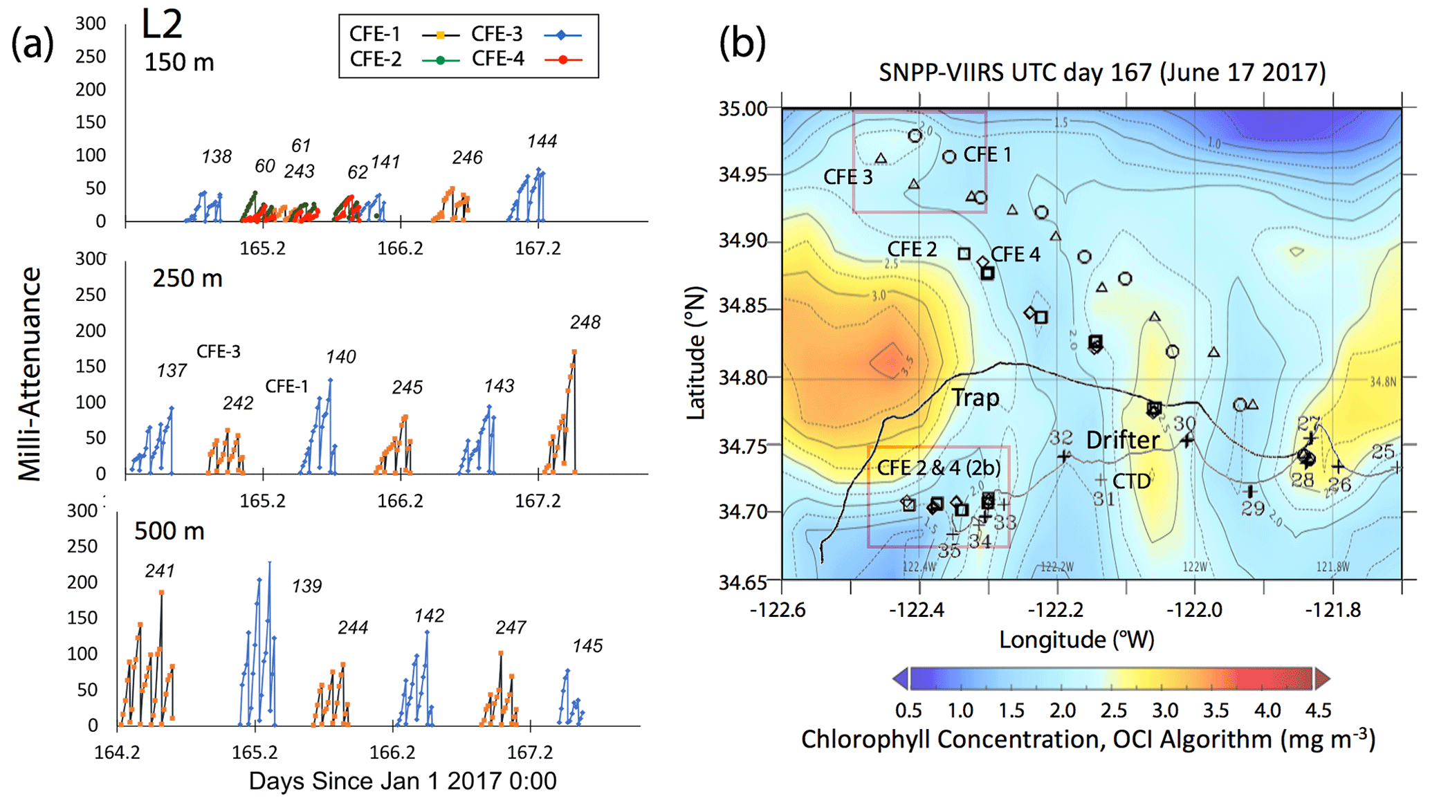
Figure 5(a) Raw attenuance time series for all CFEs deployed at L2. See Fig. 2 for deployment context. Italicized numbers are the dive numbers corresponding to the data. The mATN time series scales with flux as timing is constant. (b) Map showing deployment and trajectories of CFEs, CTD station locations, and tracks of the productivity drifter and sediment trap array during the intensive studies at L2. CFE-1–4 are indicated by circle, square, triangle, and diamond symbols, respectively. The overlay is the SNPP VIIRS chlorophyll field for 17 June 2017 during the later stages of sampling at this location.
2.2 Carbon flux explorer (CFE)
The CFE and the operation of its particle flux sensing optical sedimentation recorder (OSR) have been discussed in detail in Bishop et al. (2016). Briefly, once deployed, the CFE dives below the surface to obtain observations at target depths as it drifts with currents. The OSR wakes once the CFE has reached the target depth. On first wake-up on a given CFE dive, the sample stage is flushed with water, and images of the particle-free stage are obtained. Over time, particles settle through a 1 cm opening hexagonal-celled light baffle into a high-aspect ratio (75∘ slope) funnel assembly before landing on a 2.54 cm diameter glass sample stage. At 25 min intervals, particles are imaged at 13 µm resolution in three lighting modes: dark field, transmitted, and transmitted-cross polarized. Particles build up sequentially during the imaging cycle over 1.8 h, at which time another cleaning occurs and a new reference image set is obtained; the process repeats. After ∼ 6 h at a target depth, the OSR performs a final image set, cleaning cycle, and reference image set, and the CFE surfaces to report GPS position, CTD profile data, and OSR engineering data and then dives again.
Four CFEs were deployed pair-wise at each of the four locations (Figs. 2 and 3; Table 1). Two CFEs, referred to here as CFE-Cals (CFE-2 and CFE-4), were built to collect calibration samples as described in Bourne et al. (2019). These new CFEs were built with SOLO-II floats, with a 3-fold greater buoyancy adjustment capability than the older CFEs (CFE-1, and CFE-3) which could not carry the samplers. CFE-Cals were programmed to drift at 150 m and were typically deployed twice for 20 h at each location. We found that the concave bladder housing of the SOLO-II float trapped air in a way that made it more difficult for the CFE-Cals to attain a stable target depth. This was a particular problem when the CFEs were launched in calm conditions. We found that copious seawater rinsing of the CFE-Cal SOLO II bladder assembly prior to launch and ensuring that the CFE-Cals were horizontal when released solved this problem. The two other CFEs, CFE-1 and CFE-3, were programmed to drift at three depths (CFE-1 and CFE-3 are referred to as profiling CFEs) and did not have depth stability issues. At L1, bottom depth was ∼ 450 m, and we limited CFE dives to shallower than 300 m. At offshore locations L2, L3, and L4 the three target depths were 150, 250, and 500 m. The profiling CFEs (CFE-1 and CFE-3) were deployed at each location for 3 to 4 d. At L3, CFE-3 was attacked violently twice by a large (length greater than the 2.3 m height of the CFE with antennas) short-fin Mako shark as we watched. The first high-velocity charge hit the OSR directly and had no effect on the CFE; the second charge hit the SOLO top cap and antenna assembly and broke the float, causing CFE-3 to sink in seconds. Consequently, only CFE-1 made flux observations deeper than 150 m at L3 and L4. We deployed CFEs 24 times; 21 yielded results reported here (Table 1); two early deployments of CFE-Cals were not useful, and imagery from CFE-3 at L3 was lost due to the shark attack.
Table 1Carbon flux explorer deployments during CCE-LTER process study P1706 2 June–1 July 2017.
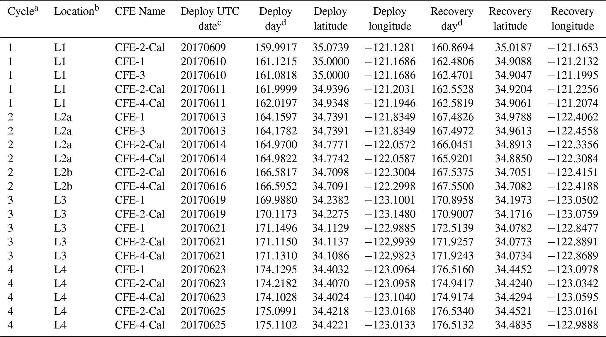
a CCE-LTER cycle number. b Location number used in this paper. c Deploy date (YYYYMMDD). d Day – year days since 1 January 2017 00:00 UTC. 1 January 2017 at 12:00 UTC = 0.5.
2.2.1 Reduction of OSR transmitted light images
Transmitted light colour images were normalized by an in situ composite image of the clean sample stage following Bishop et al. (2016), yielding a map of fractional transmission corrected for inhomogeneities of the light source. Attenuance (ATN) values were then calculated by taking the −log 10 of the normalized image using the green colour plane. Pixels with an attenuance value less than 0.02 were defined to be background. Pixels above the threshold were integrated across the sample stage and then divided by total number of pixels in the sample stage area to yield attenuance (ATN). Figure 5 depicts time series of attenuance (in mATN units) at different depths for the mid-filament location L2; similar data from L1, L3, and L4 are in Figs. A1, A2, and A3, respectively. The sawtooth attenuance trends in Fig. 5 reflect progressive particle accumulation on the imaging stage followed by stage cleaning which brings attenuance back down to baseline. Multiplying attenuance by the sample stage area (5.07 cm2) gives sample volume attenuance (VA, units: mATN-cm2; Bourne et al., 2019). VA can be thought of as the optical volume of particles on the sample stage. In this paper we focus on light attenuance (derived from transmitted light images) as a proxy of carbon flux because the proxy has been calibrated (Bourne et al., 2019).
2.2.2 Conversion of volume attenuance to POC flux
Volume attenuance (VA) has been calibrated in terms of particulate organic carbon and nitrogen (POC and PN) loading (Bourne et al., 2019). VA is converted to volume attenuance flux (VAF) by normalizing VA by deployment time and scaling by the area of the funnel opening. The regression for measured POC flux (mmol C m−2 d−1) against VAF (mATN-cm2 cm−2 d−1) is given by Eq. (2) (Bourne et al., 2019).
VAF is ∼ 4 times more precisely determined than POC flux (Bourne et al., 2019), and thus we use it as the x-axis variable. The regression R2=0.897 and the ± values denote 1 standard deviation of slope and intercept, respectively. For simplicity, we use a conversion factor of 1.0 to scale VAF to POC flux. The intercept is not significantly different from zero and is ignored. The CFE-derived optical proxy for POC flux is referred to as POCATN flux below.
2.2.3 Particle size distributions
Three methods were used to determine particle size distributions in CFE imagery: (1) a computationally efficient code that measures particle area and attenuance (Bourne, 2018), (2) manual identification and counting of particle classes, and (3) a hybrid of image analysis and visual verification of identified particles.
Transmitted light images from the CFEs were processed to attenuance units following Bishop et al. (2016). Results were saved as imagery in attenuance units where counts in each 8-bit (red, green, blue) colour plane are scaled so that 100 counts = 1 attenuance unit. The complete set of 1600 CFE transmitted light images and corresponding attenuance images are available through the Biological and Chemical Oceanography Data Management Office (BCO-DMO) at the Woods Hole Oceanographic Institution (Bishop, 2020a).
For size analysis, the RGB image is converted to an 8-bit grayscale image. The 5 MP SUMIX imager used in the CFE employs a Bayer filter that allocates in a checkerboard pattern 50 % of the pixels to green and 25 % to each of the blue and red colour channels. In the case of transmitted light imagery, we have found little difference in attenuance values from the three colour planes (Bourne et al., 2019); however, this is not true of imagery in dark-field illumination. We choose to set the definition of a “particle” as having 4 contiguous pixels above threshold in order to provide compatibility with interpretation of dark-field imagery, where colour is important. A 4-pixel particle has an area of 676 µm2 or an equivalent circular diameter (ECD) of 29 µm.
Method 1 – threshold variation
Bourne (2018) developed a computationally efficient nearest-neighbour particle detection algorithm to measure attenuance size distributions in CFE images. This was an important first step towards fully autonomous observations as this scheme can run aboard the CFE. Unlike the “stage” integration (Sect. 2.2.1), particle size analysis requires a choice of an attenuance count threshold to distinguish particles and differentiate them from background. Choosing too low of a threshold can increase the false detection of particles due to imperfections of lighting and sensor noise. Bourne (2018) studied thresholds from 0.02 to 0.20 attenuance units. Even at the highest threshold setting, the method failed to separate touching 250 µm ECD ovoid faecal pellets (Fig. 6) which constituted a significant component of particle flux at 150 m at L2. In this method, as well as method 3 (below), particle size distributions were determined in the last image of a cycle before the imaging stage was cleaned. If overlapping particles were present, the previous image in the series would be used instead. This choice was made manually but could be automated. Bourne (2018) used a threshold attenuance of 0.12 to systematically analyse 143 image cycles using this method.

Figure 6(a) Segment of a CFE-2 transmitted light image June 2017 at 19:42 UTC; depth 150 m. (b–e) ImageJ particle outline maps at attenuance thresholds of 0.02, 0.04, 0.12, and 0.20, superimposed on the attenuance image for the sample. Darker greys denote higher attenuance. We found that touching faecal pellets could not be separated even at a threshold of 0.20 ATN. At thresholds >0.06, large low-density aggregates are seen as highly fragmented, and the contribution of smaller particles is reduced. (f) Particle size attenuance count distributions as a function of threshold. (g) Magnified image under dark-field illumination. Olive-coloured faecal pellets are readily distinguished from an unidentified egg. (h) Attenuance map of the same view.
Method 2 – manual counting
CFE images from L2 were manually enumerated for ovoid faecal pellets and > 1000 µm sized aggregates using a combination of transmitted light and dark-field imagery (Connors et al., 2018; Bourne et al., 2019).
Method 3 – ImageJ size analysis and secondary processing
In method 3, the software package ImageJ 1.52 (IJ, National Institutes of Health) was used for particle size analysis. The advantage of ImageJ is that the analysis provides a rich statistical description of the individual particles that can be used to aid in particle class analysis. In this method, we manually inspected the four to five sequential attenuance images taken during each image cycle to determine the point of onset of particle overlap. The attenuance image was subtracted from the preceding attenuance image of the clean sample stage. A threshold of four counts (0.04 ATN) and above was used to define the presence of particles (two counts higher than used for calculation of VA). At this threshold setting, large aggregates were fully detected; however, touching particles – particularly 200–400 µm sized faecal pellets (Fig. 6) were not separable. Each IJ-identified “particle” with multiple identical units was counted, and these counts were assigned to its sequence number. Inspection of the imagery also identified touching large aggregates which were similarly treated. During secondary data processing, the area of each multi-unit “particle” was divided by the number of subunits, and its particle number was changed from 1 to the determined count. Examples of touching ovoid particles are found in Fig. 6. Living organisms rarely appeared in images; when they did appear, we were able to identify pteropods, amphipods, copepods, siphonophores, acantharia, radiolaria, and foraminifera. These “living” particles were removed from the secondary processed data. Total particle attenuance (average particle attenuance times particle area) and particle number were binned into 65 logarithmically spaced size categories from (30 to 20 000 µm). A total of 267 image pairs were analysed; these combined flux results for each of 89 CFE dives are available online through the Biological and Chemical Oceanography Data Management Office (BCO-DMO; Bishop, 2020b). Float CTD results are similarly archived (Bishop, 2020c).
Data from each image cycle were weighted by the total number of images in that cycle; data from the multiple imaging–cleaning cycles during a dive were binned and weighted by the duration of each imaging cycle. The particle attenuance and number-size-binned data were scaled to convert results to flux units (mATN–cm2 cm−2 d−1 and number m−2 d−1). The partitioning of particle flux by size was simplified to five size categories: 30–100, 100–200, 200–400, 400–1000, and > 1000 µm. In the process, ATN and number fluxes at category boundaries were determined by interpolation of the detailed cumulative flux–size distributions. The 200–400 µm bin was primarily populated by the numerous ovoid pellets. The > 1000 µm bin was dominated by aggregates.
Figure 7 displays normalized cumulative size distributions prior to and after secondary processing for all CFE dives at L2. The point of this labour-intensive computer-aided approach was to provide a basis for future code development. The scientific outcome of this analysis is a description of the number and attenuance fluxes of differently sized particles and how these fluxes change down the water column during the CCE-LTER process study.
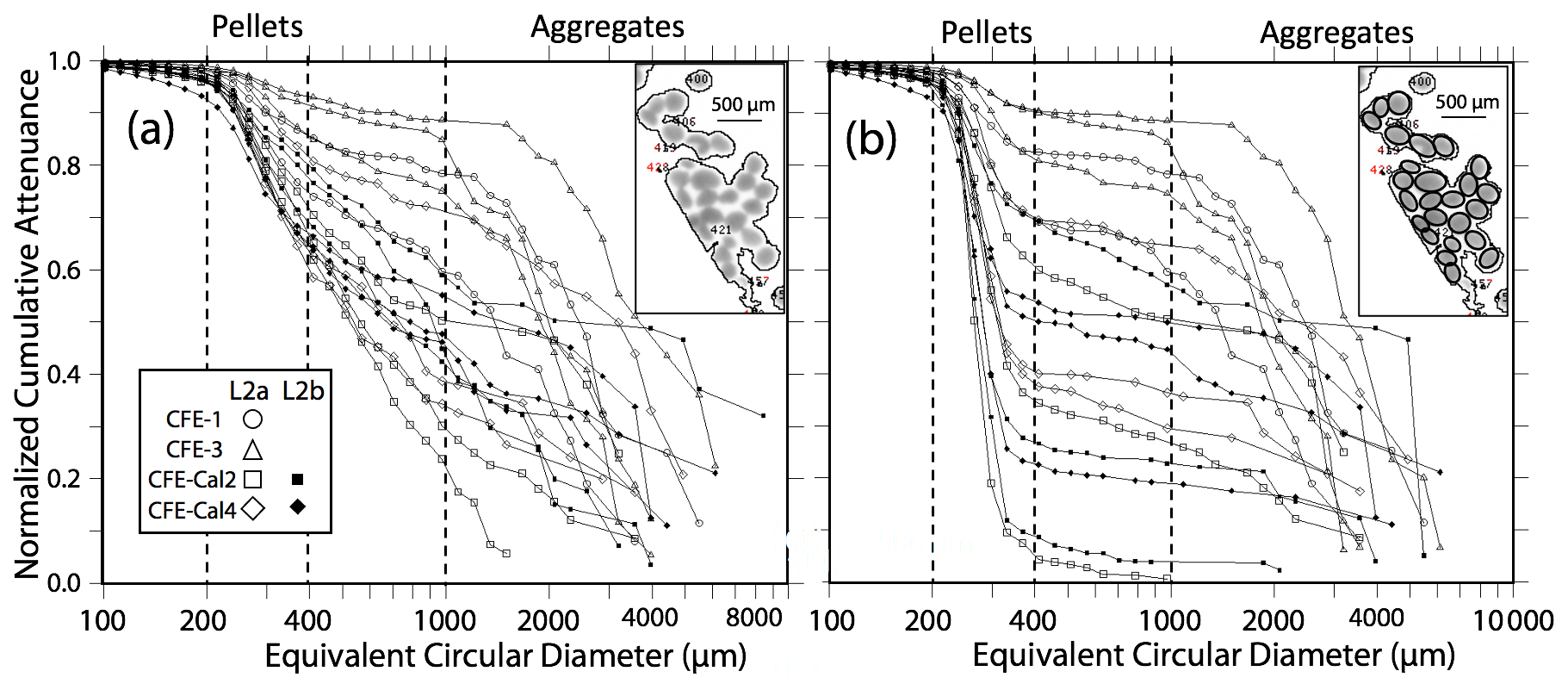
Figure 7Processed size distribution data for CFE-1–4 deployed near 150 m at L2. Normalized cumulative attenuance flux is plotted against equivalent circular diameter (µm). (a) Original cumulative attenuance size distributions from ImageJ and (b) after secondary processing to correct for touching particles (see insets in upper right-hand corners of a and b). Boundaries for reduced size categories are 30–100 (not shown), 100–200, 200–400, 400–1000, and >1000 µm and are indicated in (a) and (b). Open and closed symbols denote data from the first and second deployments of the CFE-Cals at location 2 designated as L2a and L2b, respectively. After correction, the 400–1000 µm size category contributed little to sample attenuance.
Method intercomparison
Figure A4 compares normalized-cumulative-attenuance flux and normalized-cumulative-number flux size distributions from methods 1 and 3 at locations L1–L4. Some differences are attributed to independent choices of which image sets to analyse (137 vs. 267) using the two methods; nevertheless, we found good agreement between the methods for data from 250 m and deeper. The poorer agreement in size distributions from 150 m is due to the high threshold (0.12 attenuance) of method 1 failing to detect large aggregates as whole particles and also the problem of touching faecal pellets, which dominated samples at 150 m at L2 (Fig. 6).
Figure 8 compares profiles of aggregate (> 1000 µm) and pellet (200–400 µm) number fluxes with manually determined counts of these classes at location L2. Although the data were calculated in slightly different ways, method 3 aggregate flux and manually determined aggregate flux closely matched. The method 3 pellet flux agreed closely with manual counts at 150 m but overestimated results at 500 m by a factor of 5. To understand this difference, we graphed particle attenuance for all 150–400 µm sized particles at 150 m at L2. Results showed a cluster of particles > 200 µm in size with attenuance values > 0.25, which suggested that the cluster was due to ovoid faecal pellets. We calculated the ratio of the number of particles > 0.25 attenuance to total particles and used the ratio to correct the method 3 counts. Results brought the method 2 and method 3 counts at L2 into agreement (Appendix A, Table A1). We applied this approach to L1, L3, and L4 data (Fig. 8). L4, in particular, showed high numbers of particles in the 200–400 µm category which originated from the fragmentation of large low attenuance aggregates; only 15 % of particles had attenuance above 0.25 at 250 and 500 m.
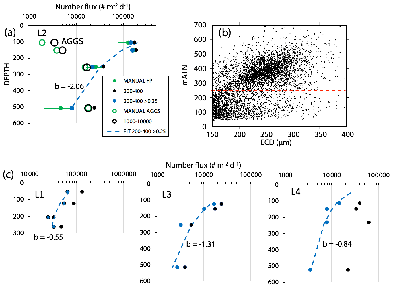
Figure 8(a) Profile of aggregate and pellet number fluxes determined by method 3 and by manual counting at Location L2. The small blue-filled circles represent number flux of 200–400 µm particles with average attenuance >0.25. These data agree closely with manually enumerated pellet counts. Method 3 counted more aggregates in the shallowest samples because the manual method was unable to infer weakly defined boundaries of less dense aggregates. Data are tabulated in Appendix A, Table A1. (b) Plot of average particle attenuance vs. equivalent circular diameter (ECD). The red dashed line denotes the lower boundary of the cluster of >0.25 ATN particles. (c) Profiles of 200–400 µm total particle number fluxes and for >0.25 ATN particles at L1, L3, and L4. Dashed lines are Martin fits to the ovoid pellet class fluxes. In all cases, fluxes of faecal pellets decrease with depth.
2.2.4 Sources of uncertainty of POCATN flux
Calibration studies by Bourne et al. (2019) were restricted to depths near 150 m due to logistical reasons including ship time, the need for replication of results, and the need for comparison of POCATN fluxes with data from surface-drogued sediment traps (Sect. 2.4 below) which were restricted to the upper 150 m. We do not believe that this is a major limitation because samples collected at 150 m covered a wide range of size distribution and particle types that were also found deeper in the water column. Furthermore, large particles sampled by large-volume in situ filtration show little shift in organic carbon percentages from the base of the euphotic zone to 500 m (e.g. Bishop et al., 1986). For these reasons, we assume that the uncertainty of our present calibration is ∼ 9 % (± 1 SD; Eq. 2). More calibration sampling is desired.
During review, we were asked to estimate the contribution of counting statistics to the uncertainty of POCATN flux for the > 1000 µm particle class vs. that for smaller size classes. As we show below that the large aggregate size fraction dominates total POCATN flux, it is also true that this flux is determined by a relatively small number of aggregates arriving during each image cycle. We assume Poisson counting statistics, where the relative standard deviation (RSD) counting error for n particles is , and that the RSD can be applied to both number flux and attenuance flux. Figure A5a shows representation of this error for the 200–400 µm and > 1000 µm categories; two cases are calculated: that for individual dive results and that for the grand average of all dives at four depth horizons at each location. Count-related errors for individual dives for the 200–400 and > 1000 µm categories were typically < 10 % and < 30 %, respectively; similarly, for pooled dive results such errors were typically < 5 % and 20 %. At L3 where fluxes were low, count-related errors for POCATN flux in 200–400 and for > 1000 µm categories were typically 20 % and 40 %, respectively; pooled results gave ∼ 15 % and 30 % errors. Figure A5b illustrates the combined effect of counting error and 9 % calibration uncertainty for individual dives at L2 and L3 (as plotted in Fig. 15a below). These errors are minor compared to the range of POCATN flux values observed. The complete dive-averaged data sets with error estimates are available as supplemental online material. Note n values used for error calculation listed in the supplemental data set are not integers due to number fluxes being based on extrapolations to the boundaries of the five size categories.
We assume for the following discussion that the VAF : POC flux relationship has a 9 % uncertainty and is invariant with depth; furthermore, errors due to the statistical frequency of particles in different size categories are also deemed a minor influence on our interpretations.
2.3 Acoustic Doppler current profiler (ADCP) and other CTD data
Current velocity in u (east positive) and v (north positive) components from the hull-mounted RD instruments 150 kHz narrowband acoustic Doppler current profiler (ADCP) were averaged over 30 min intervals during the times of CFE deployment. The 150 kHz data were limited to the upper 400 m. CFE drift velocities were calculated based on CFE dive locations and times. Combined ADCP and CFE drift results are shown in Fig. 9.

Figure 9The 30 s averaged current velocities in u (east positive) and v (north positive) directions from 150 kHz narrow band ADCP data. CFE depths during flux measurements are shown. Profiles denoted by black asterisks to right of each contour plot are averaged ADCP velocities for the entire time span. Red points represent average CFE velocities over the course of each dive. Shaded boxes denote missing data. Filled blue triangles are the averaged CFE velocities for all dives at a given depth. Panels (a), (b), (c), (d), and (e) Locations 1, 2a, 2b, 3 and 4 respectively.
The hydrographic context for our study was provided by CTD profiles of T, S, potential density anomaly (σθ), photosynthetically active radiation (PAR), chlorophyll fluorescence (Seapoint Sensors Inc.), turbidity at 810 nm (Seapoint Inc.), and transmission at 650 nm (WET Labs, Inc. Philomath, OR). Particle optics were kept clean as detailed in Bishop and Wood (2008). The CTD–rosette casts were usually made in close proximity to a surface-drogued productivity array which served as the Lagrangian reference for studies at each location. Nutrient data from the CTD–rosette samples used in this paper are archived in the CCE-LTER data repository (https://oceaninformatics.ucsd.edu/datazoo/catalogs/ccelter/datasets, last access: July 2018).
Transmissometer-derived beam attenuation coefficient (m−1) multiplied by a factor of 27 is used to calculate particulate organic carbon (POC) concentration (µM; Bishop and Wood, 2008). The Seapoint fluorescence data were offset by subtraction of 0.05 units, and residual values lower than 0.02 were determined to be below detection. The CTD–rosette also carried an underwater vision profiler particle imaging system (UVP5-hd; Hydro-Optic, France) capable of resolving particles > 64 µm in reflected light. Data are archived at https://ecotaxa.obs-vlfr.fr/part/, last access: December 2018, under the project UVP5hd CCELTER 2017. We used the “non-living” particle concentrations averaged over 5 m, which were representative of particles present in ∼ 180 L. We pooled and further depth-averaged all CTD cast data at each location to achieve an equivalent water volume of ∼ 2000 L to improve the statistics of the number concentrations of > 1000 µm aggregates. In this paper we focus on the > 1000 µm fraction, although all size fractions have been treated identically. Further detailed analyses of UVP5 imagery are beyond the scope of the paper.
2.4 New-production-based carbon export (POCNP flux) and particle interceptor trap flux
Euphotic zone new production (NP) measurements at locations L1, L2, L3, and L4 (converted to carbon units) were 189 ± 21, 156 ± 77, 63 ± 33, and 19 ± 3 mmol C m−2 d−1, respectively (Kranz et al., 2020). We refer to these data as POCNP flux. POC fluxes from deployments of surface-drogued particle interceptor traps (PITs) traps deployed to 150 m are from Stukel and Landry (2020). These values are referred to as POCPIT flux.
In this study, CFEs were programmed to dive deeper than 100 m, and POCATN fluxes were lower than POCNP values at all locations except at L4, the last occupation of the filament; in this case POCATN flux exceeded POCNP by a factor of > 2 at 250 m, suggesting a recent decline in carbon export. Nitrate and beam attenuation coefficient (POC) changes (Table 2) allow an estimate POCNP flux for the 9 d interval spanning the occupations of L2 and L4. We have confidence in this calculation since a sediment trap array, deployed late in the study at L2b, tracked the water to L4 (Kranz et al., 2020); furthermore, L2b and L4 salinity profiles were virtually identical (Fig. 10), confirming that the surface water masses encountered at L2 were nearly the same as at L4. Following Johnson et al. (2017), we subtract 0–45 m stocks of dissolved nitrate at L2b from L4 (Table 2) and multiply this change by the molar ratio of photic layer plankton . Johnson et al. (2017) used a ratio of 6.6; we used a of 6.4 (Stukel et al., 2013). We chose 45 m as the integration depth as dissolved nitrate profiles at the two sites converged at this depth (Fig. 10) and also because 45 m was close to the euphotic zone depth at L4. The calculation yielded an averaged POCNP flux = 111.3 ± 32.2 (SD) mmol C m−2 d−1 over 9 d, similar to measured POCNP at L2, but a factor of 6 higher than reported at L4 by Kranz et al. (2020). POC inventory changes (Table 2) from L2b to L4 between the two times implied an average POC loss rate of 33 mmol C m−2 d−1. Crustacean grazers have assimilation efficiencies of 70 %, with the remaining fraction voided as faecal pellets. Export from this POC loss would add ∼ 10 mmol C m−2 d−1. Averaged export from L2b to L4 sums to ∼ 120 mmol C m−2 d−1.
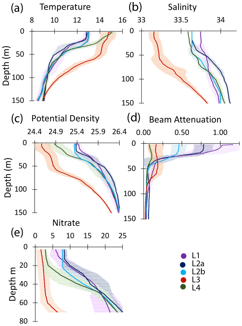
Figure 10Profiles of averaged T, S, potential density, beam attenuation coefficient (650 nm), and nitrate in the upper 150 m at locations L1, L2a, L2b, L3, and L4. Error bars are ± 1 SD.
Table 2Hydrographic and euphotic zone properties at CCE-LTER P1706 study locations.
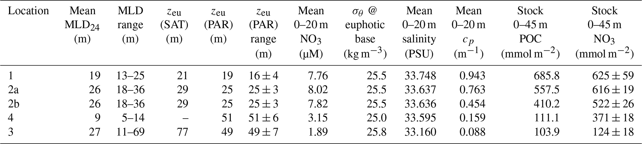
MLD24: daily average mixed-layer depth based on σθ difference = 0.05 kg m−3; zeu: euphotic zone depth based on satellite (SAT) or CTD photosynthetically active radiation (PAR) 1 % light level.
3.1 Spatial context and water column environment
CFE deployment locations and times are summarized in Table 1 (above). Table 2 summarizes mixed-layer and euphotic zone properties for each intensive study location. Figures A1b, 5 (above), A2b, and A3b show satellite-retrieved surface chlorophyll fields from SNPP VIIRS with superimposed locations of CFE surfacing and CTD/optics profiles and tracks of the surface-drogued particle interceptor trap (PIT) array and of the drogued productivity (PROD) array at locations L1–L4, respectively. At locations L1 and L4, the Lagrangian CFEs tracked well with all deployed systems; at L2, there was a divergent behaviour of CFEs, PIT, and drifters with the CFE and PIT arrays remaining closest; at L3, the CFE and PIT arrays maintained a similar track. At all locations, CFE trajectories closely matched ADCP velocities (Fig. 9) and the patterns of flow suggested by sea surface altimetry (Fig. 4).
Figure 11 shows time series depth plots of T, S, potential density (σθ), chlorophyll fluorescence, transmissometer-derived POC, and turbidity at locations L1 through L4. Figure 12 shows time series POC and S versus potential density plots at L1 through L4 as well as spatial transects of POC and salinity versus potential density. We reordered the time axis in these figures to make data from in-filament locations L1, L2, and L4 more logically related and separate from the out-of-filament transitional waters at L3. L2 is split temporally into L2a and L2b for reasons outlined below.
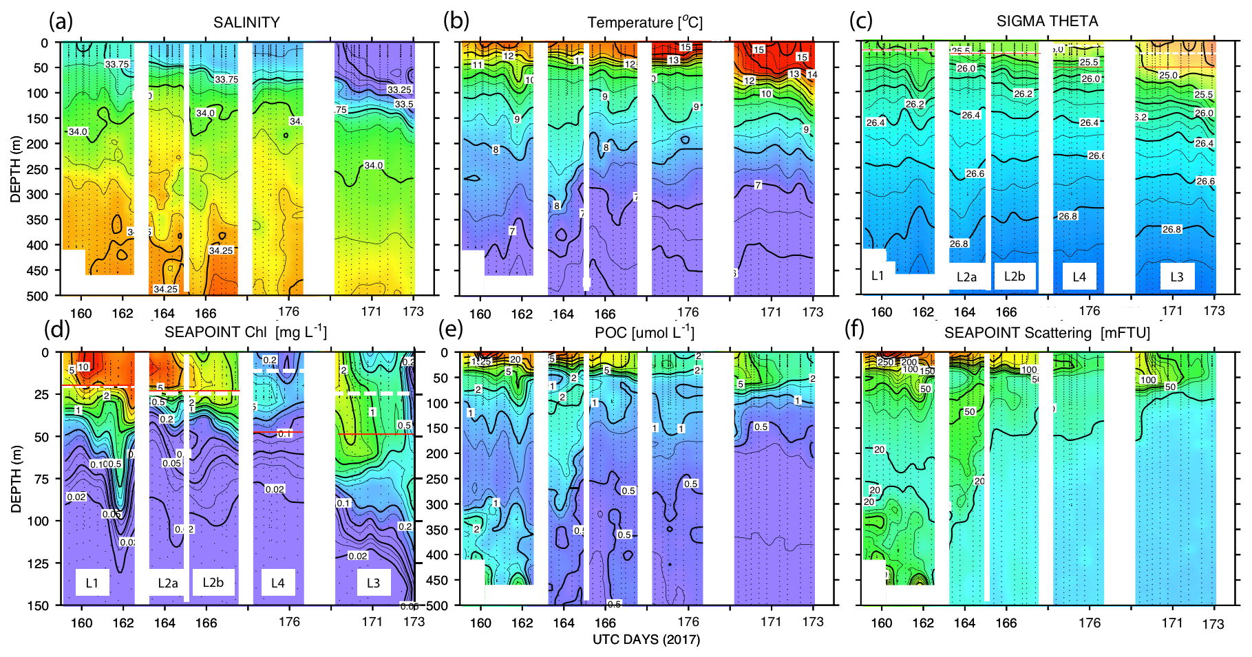
Figure 11(a) Salinity, (b) temperature, (c) sigma theta (σθ), (d) chlorophyll fluorescence, (e) transmissometer-derived POC, and (f) turbidity time series from CTD casts. The time axis (in UTC days since 1 January 00:00 2017) has been reordered so that L1, L2, and L4 are grouped. L3 is shifted to the right side of each panel. The white dashed line and red line (c) and (d) denote averaged 24 h mixed-layer depths and euphotic zone depths, respectively. The chlorophyll fluorescence (d) depth axis is 150 m; the limit of detection was 0.02 units.
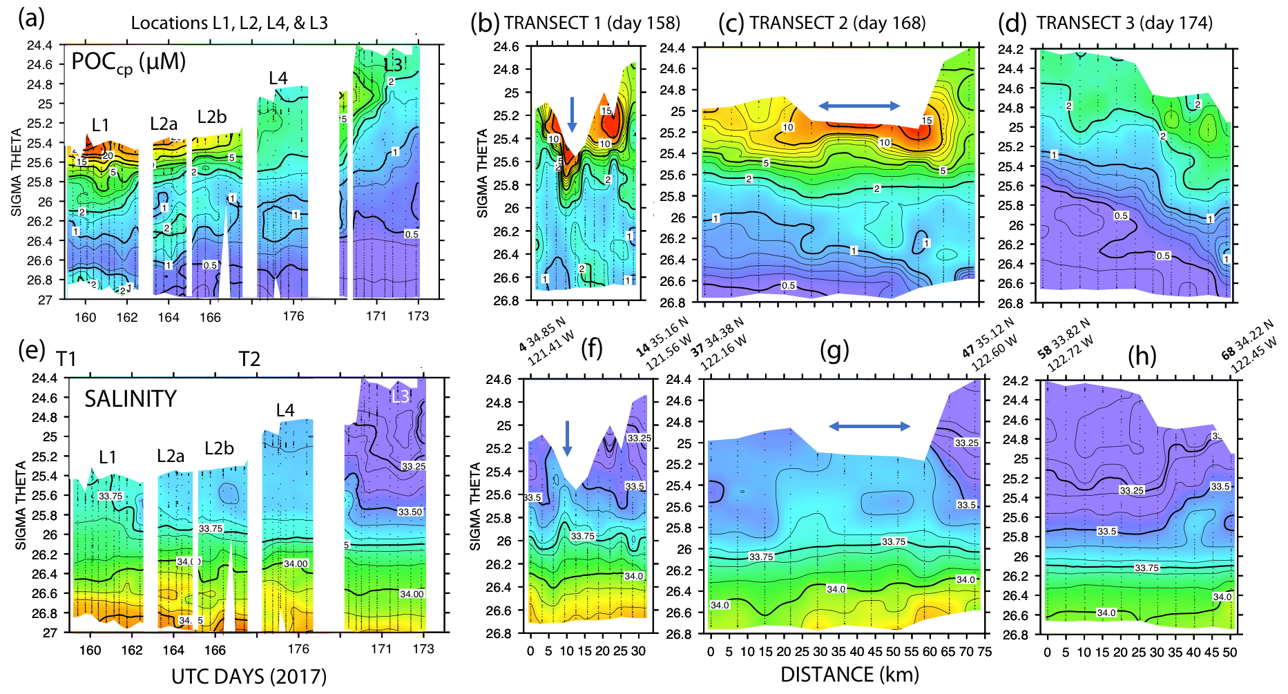
Figure 12(a) Transmissometer particulate organic carbon (POC) and (e) salinity – potential density time series during the intensive studies at L1, L2a, L2b, L4, and L3. Also shown are cross-filament transects T1, T2, and T3 for POC (b, c, d) and salinity (f, g, h). Transect locations are shown in Fig. 2. Transect T1 (UTC day 158) was located between L1 and L2; T2 (day 168) was sited between L2 and L4; and T3 crossed the outer edge of the filament on day 174 after completion of work at L4. Distances are in kilometres. UTC days as defined in Fig. 10. The arrows in (f) and (g) indicate the high-salinity surface water in the filament; its scale was ∼5 km wide at T1 and ∼25 km wide at T2.
3.1.1 Location 1
The study site L1 was located in the middle of a 50 km wide 500 m deep trough (Fig. 2) approximately 25 km offshore of Morro Bay, CA. The SNPP VIIRS chlorophyll (Fig. A1b) shows that early CFE and CFE-Cal deployments took place in close proximity to very-high-chlorophyll waters. Upwelling was active as evidenced by cold, high-salinity surface waters and low stratification (Figs. 10, 12). The 24 h mixed-layer depth (MLD24), defined by a potential density increase of 0.05 kg m−3 relative to surface values (Bishop and Wood, 2009), averaged 19 m (range from 13 to 25 m) and matched euphotic zone depth (16 ± 4 m) (Table 2). Mixed-layer nitrate dropped from 10.2 to 5.4 µM over several days. CFE attenuance time series showed an early high flux event (Fig. A1a). ADCP-derived currents (Fig. 9a) show strong tidal fluctuation; however, there was a net southwest transport of water in the upper 50 m at a velocity of 0.06 m s−1, at 0.02 m s−1 between 100 and 200 m, and at 0.04 m s−1 between 200 and 300 m. Deployed instrument trajectories were consistent with ADCP results.
3.1.2 Location 2
Site L2 was located 110 km offshore. MLD24 averaged 26 m and matched the euphotic zone depth of 25 ± 3 m. The base of the euphotic zone was bounded by the σθ=25.5 kg m−3 isopycnal. The temperature and salinity profiles from CFE-1 and CFE-3 (Bishop, 2020c) were in close agreement with CTD casts 25–30 (locations Fig. 5b), whereas the subsequent CTD cast data and CFE-1 and CFE-3 data diverge. The early CTD casts revealed a stronger halocline and pycnocline, with saltier, denser waters between about 25 and 150 m, indicating upwelling in this part of the time series (Figs. 10 and 11). We thus treat the first six CTD casts as representative of CFE deployment 2a and subsequent casts as 2b. Averaged 0–20 m nitrate was 8.6 and 7.8 µM during 2a and 2b, respectively; salinity values were identical. Chlorophyll fluorescence and transmissometer-derived POC decreased by a factor of 2 during observations at 2a and 2b (Figs. 11d and 12a). During the later stages of CFE observations, SNPP VIIRS surface chlorophyll fields were almost uniform (1.8 to 2.5 mg chl a m−3; Fig. 5b).
CFE-1 and CFE-3 were launched in a fast-moving part of the filament and transported to the WNW (Fig. 5b) and separated from the surface-drogued PIT array and productivity drifter; 20 h later, CFE-Cals 2 and 4 similarly tracked to the WNW on a parallel course to CFE-1 and CFE-3 (Fig. 5b). When redeployed a day later near the drifter, CFE-Cals 2 and 4 advected to the west but at a greatly reduced speed, indicating that the upper 200 m had become decoupled from the faster flow tracked by CFE-1 and CFE-3. During L2a, ADCP data showed a consistent net west-northwest current velocity at 0.17 m s−1 in the upper 50 m, an increase to 0.29 m s−1 between 100 and 200 m, and 0.27 m s−1 between 200 and 300 m (Fig. 9b); CFE motions were used to infer a velocity of 0.15 m s−1 at 500 m. During L2b, the current direction was to the west, but velocities were reduced at all depths (0.04 m s−1 in the upper 50 m, 0.11 m s−1 between 100 and 200 m, and 0.12 m s−1 between 200 and 300 m; Fig. 9c).
3.1.3 Location 3
L3 was located 240 km offshore in transitional waters between the westward-extending filament and the surrounding southerly flowing waters of the California Current. The MLD24 at L3 averaged 27 m (range 11–69 m). The euphotic zone was at least twice as deep as the MLD24 (77 m NASA VIIRS; 49 ± 7 m from PAR profiles, Table 2). The base of the euphotic zone was bounded by the σθ=25.75 kg m−3 isopycnal. CFE-1 and CFE-3 and CFE-Cal-2 were launched but recalled within 24 h for repositioning as CTD cast data indicated a relatively strong influence of the filament. CFE-3 was lost at this time. CFE-1 and CFE-Cals 2 and 4 were redeployed approximately 10 km to the south of the first deployment locations.
Salinity of the upper 50 m at L3 decreased over time from 33.35 to less than 33.2 PSU, indicating an increasing component of the southerly flowing low-salinity California Current water (Schneider et al., 2005). Surface layer nitrate averaged 1.9 µM. CFE flux indicators were low (Fig. A3a). Current flow was to the southeast at L3 with 0.30 m s−1 velocities in the upper 50 m, 0.14 m s−1 between 100 and 200 m, and 0.08 m s−1 between 200 and 300 m (Fig. 9d). CFE drift at 500 m was 0.07 m s−1. CFE trajectories followed the path of the PIT array but at a slower speed.
3.1.4 Location 4
This site (235 km offshore) was located ∼ 35 km north of L3 in the western extension of the filament (Fig. 3g, h). Based on the salinity signature of L2b and L4, the water masses were similar (Table 2, Fig. 10). SNPP VIIRS chlorophyll data (Fig. A3b) show low and nearly uniform chlorophyll (0.25 mg m−3) in the vicinity of observations. Surface nitrate was depleted, and sea surface temperature had increased due to solar heating (Figs. 3h, 10). MLD24 averaged 9 m; euphotic depth was 51 ± 6 m. The euphotic zone base corresponded to the σθ=25.0 isopycnal. ADCP currents were to the northeast at 0.11 m s−1 in the upper 50 m, decreasing to 0.04 m s−1 between 100 and 200 m, and 0.02 m s−1 between 200 and 300 m; at 500 m, a velocity of 0.03 m s−1 was calculated from CFE drift displacements.
A reasonable assumption is that the average salinity of the surface layer (here defined as upper 20 m) at L2 and L4 is a result of binary mixing of recently upwelled L1 water with the California Current water at L3. Using data in Table 2, we calculate that surface waters at L2a were an 81.1 : 18.9 % mixture of L1 and L3 waters; similarly, L2b was 80.9 : 19.1 %, and L4 was 74 : 26 %. As the filament moved over 200 km offshore it remained mostly hydrographically distinct.
3.2 Sinking particle lateral displacements
One of the questions raised in particle flux measurement is as follows: how well are fluxes at depth related to measured surface layer export? As an exercise we consider particles sinking at a hypothetical rate of 100 m d−1 from 50 m to depths of 150, 250, and 500 m and their lateral displacements during sinking at the four locations. Figure 13 visualizes such displacements.

Figure 13Displacements (in kilometres) in the direction of motion of the filament for particles with a hypothetical sinking rate of 100 m d−1 as they sink from 50 m. Extreme displacements were calculated for transitional waters (L3) where sinking particles lagged behind the surface layer by as much as 85 km. Sinking particles would lead the surface layer by 20 km at a depth of 250 m at L2a. Calculated from ADCP velocities in Fig. 9.
CFE positions followed a near-linear trajectory in time at many locations despite drifting at different depths; trajectories were in close agreement with ADCP current velocities (Fig. 9). The linearity of track allows a simple calculation of displacements in the direction of motion. At L1, ADCP velocity data (discussed in Sect. 3.1) indicate that particles sinking at 100 m d−1 would lag behind the surface layer by 7 km as they transited from 50 to 300 m. At L2a, particles leaving 50 m would lead the surface layer by 11 km by the time they arrived at 150 m; they would lead surface waters by a total of 19 km by 250 m; particles would lag the 250 m layer by 4.5 km on reaching 500 m. Taken together, particles sinking from 50 m would have a net displacement of 15 km relative to the surface layer. At L2b, in a weaker current regime, sinking particles would lead the surface layer by 6 km during transit to 150 m and have a total displacement lead of 12.5 km by 250 m. At L3, in transitional waters, particles would lag behind the motion of surface waters by 14 km by 150 m and lag surface waters by 83 km on arrival at 500 m. At L4, particles settling at 100 m d−1 would lag behind the 50 m layer by 3.5 km on reaching 150 m and would have a total displacement of 13 km by 500 m.
In summary, inferred lateral displacements were calculated relative to the direction of flow of surface waters as particles sink from 50 m to deeper waters. The smallest net displacements of sinking particles was found at L1 (7 km, 300 m), L4 (13 km, 500 m), and L2a (14 km, 500 m). Location L3 in the transitional waters had the strongest net displacements (83 km) by 500 m, making a 1D interpretation of particle flux most problematic at this location. An interesting feature of L2 is that particles at depth would lead the surface layer. Displacements of particles sinking at a different velocity, V, would scale by .
Particle flux profiles observed by the CFEs may reflect heterogeneous sources over the scales of displacement. If spatial gradients of particle sources along the axis of the plume are weak, then the vertical lead and lag effects will be in effect smaller. SNPP VIIRS chlorophyll fields provide a measure of mesoscale chlorophyll variability at location L2. Imagery from 14 June during the early stages of sampling show chlorophyll varying over a range of 3 to 1.75 mg chl m−3 along the path of the profiling CFEs. Imagery from 17 June showed a variation of 2.5 to 1.75 mg chl m−3 (Fig. 5b) along the same track. The two images for 14 and 17 June show ranges of 2.25 to 2.75 and 1.75 to 2.25 mg chl m−3, respectively, in the vicinity of the later deployment of CFEs (waters referred to as L2b). If chlorophyll is a metric of particle flux, then spatially variable fluxes would be expected to vary by less than a factor of 2 at L2. Similar maps for L1, L3, and L4 (Figs. A1, A2, and A3) indicate the likelihood of heterogenous fluxes at L1 and L3 but minimal heterogeneity at L4.
3.3 Particle classes and size-dependent POCATN fluxes
Figure 14 shows representative CFE imagery (selected from the 1250 images) taken at the four locations at depths of 70, 125, and 250 m at L1 and at depths of 150, 250, and 500 m at the other locations. The dominant class of particles contributing to export at each location varied. Shallow export flux through 100 m at L1 was dominated by 7–10 mm long optically dense anchovy pellets (Fig. 14); at L2 copepod pellets (Figs. 14, 6g, h, 8a) accounted on average for 50% of the flux (range 10 % to 90 %; Fig. 7b) with > 1000 µm aggregates (Figs. 6, 14) accounting for the rest. At L3 and L4, export was dominated at all depths by > 1000 µm sized aggregates. Large > 1000 µm sized aggregates resembling discarded larvacean houses were common at all sites at depths 250 m and below. We infer their origin based on size and morphology. Such aggregates were also present in samples closer to the surface, though not typically as abundant.
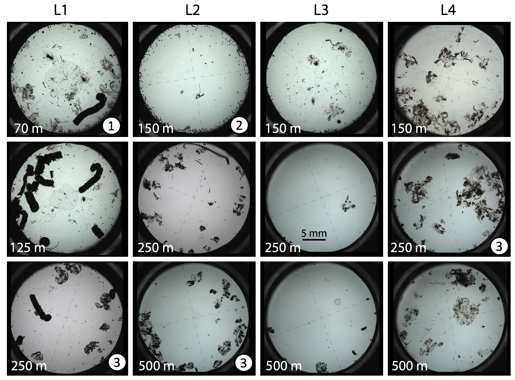
Figure 14Representative transmitted light imagery of particles sampled by the CFEs at locations L1, L2, L3, and L4. The top row of images is for material captured shallower than ∼150 m. The middle row shows particles captured near 250 m (125 m at L1). The bottom row are images of particles captured near 500 m (250 m at L1). Dashes in the images are 1 mm long. Anchovy faecal pellets are the optically dense 7–10 mm long particles seen in images at L1 (1). The 150 m sample at L2 is ringed by several hundred ∼250 µm sized olive faecal pellets (2). The >1000 µm sized aggregate particles dominate deeper samples at all locations and especially so at L4 (3). A closeup of olive-coloured faecal pellets and aggregates is in Fig. 6. All imagery is available online.
Volume attenuance flux was converted to POCATN flux (1 VAF unit = 1 mmol C m−2 d−1, Sect. 2.2.2) and partitioned into 30–100, 100–200, 200–400, 400–1000, and > 1000 µm size categories for 21 CFE deployments at the four locations. Martin curve parameters were derived from linear least-squares fit to the log10 transforms of the data according to Eq. (3):
F is POCATN flux at depth z, b is the Martin power, and zref was set to 50 m at L1 and 100 m at L2, L3, and L4. FRef is calculated from the intercept. It should be noted that Martin b values are independent of the reference depth chosen. As is precisely known, it is chosen as the X variable. Table 3 summarizes Martin fit results for POCATN flux. Table 4 summarizes Martin parameters for PIT-derived carbon flux (POCPIT flux) and to POCPIT flux combined with a new-production-based estimate euphotic zone carbon export (POCNP flux) (Kranz et al., 2020; Stukel and Landry, 2020); zref was set to the euphotic zone depth. Table 5 is a tabulation of Martin fit results for particle number fluxes across the different size categories. Data used for regressions are provided as the Supplement.
Table 3Martin curve fits to attenuance flux (all dives).
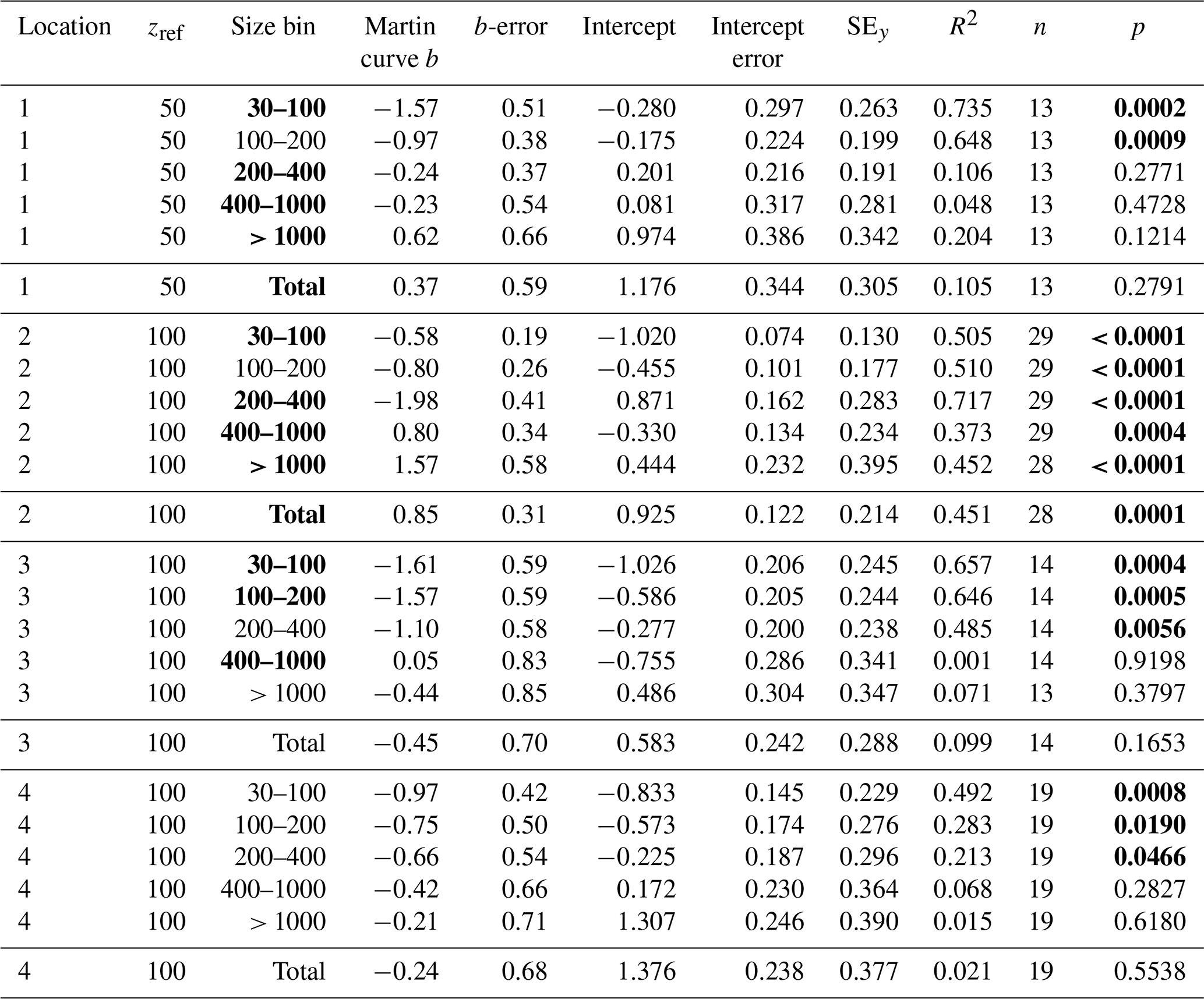
Notes: b and intercept errors are 95 % confidence intervals, and p denotes the probability that slope is zero. Bold: < 0.05.
Table 4Martin curve parameters for PIT trap data (zref: euphotic depth).
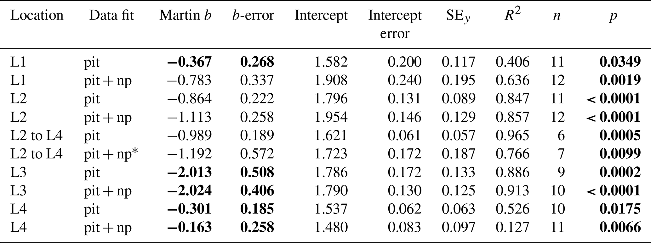
Notes: errors are 95 % confidence intervals. Bold: p < 0.05 or b significantly different from Martin . p denotes the probability that slope is zero. * New-production-based POC export is estimated NO3 inventory change between L2 and L4.
Table 5Martin curve fits to number flux (all dives).

Notes: b and intercept errors are 95 % confidence intervals. p denotes the probability that slope is zero. Bold: < 0.05.
Figure 15a shows POCATN flux for individual dives partitioned by particle size class. Martin fits to the data are also shown (Table 3). Figure 15b shows the fraction of POCATN flux for each size category. Large symbols denote pooled data at four depth horizons. POCATN flux decreases with depth at all locations for particles in the 30–100, 100–200, and 200–400 µm categories, often close to the classic Martin function (Table 3). Our refinement of the 200–400 µm fraction which separated the high-attenuance ovoid faecal pellets from other particles (Fig. 8) also shows that this pellet class consistently decreases down the water column at all locations. The > 1000 µm POCATN fluxes increase with depth at L1 and L2 and show little trend with depth at L4 and a slow decrease with depth at L3. Flux was dominated by > 1000 µm aggregates at all locations except at L2 near 100 m where 200–400 µm material had an equal contribution (Fig. 15b).
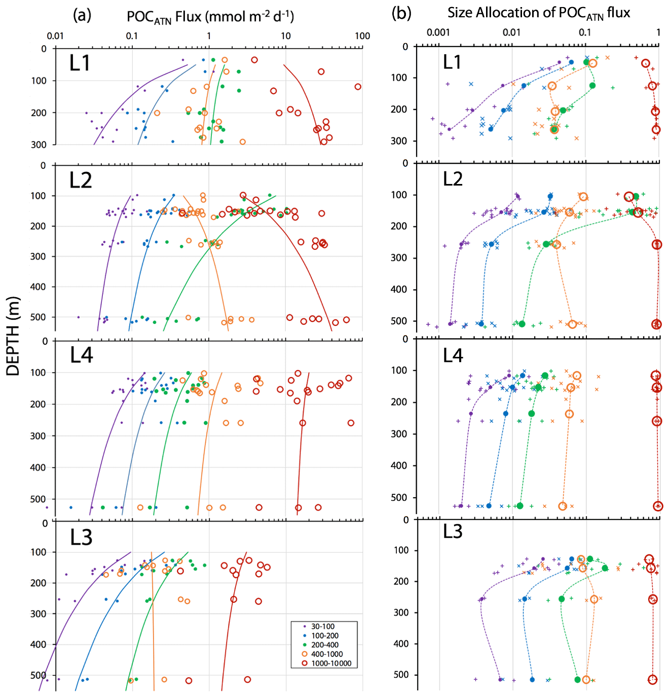
Figure 15(a) POCATN flux in mmol C m−2 d−1 partitioned in 30–100, 100–200, 200–400, 400–1000, and >1000 µm particle size classes for all CFE dives from in-filament locations L1, L2, and L4 and from transitional waters at L3. The curves denote Martin function fits to the data (Table 3). (b) Fraction of POCATN flux allocated to 30–100, 100–200, 200–400, 400–1000, and >1000 µm size fractions. Large symbols connected by dashed curves are averages of pooled data, and small points correspond to individual dives. Aggregates greater than 1000 µm in size dominated flux in all regimes with the exception of the 100 m at L2.
At L1, POCATN flux was high with significant anchovy faecal pellet contributions (Fig. 14). At location L2, the flux at 150 m was dominated by 200–400 µm sized olive-coloured ovoid faecal pellets. Number fluxes were 150 000 m−2 d−1. Evidence suggesting a fast-sinking rate for these particles was that they accumulated at the edges of the sample stage, reflecting the focusing effect of the tapered funnel (Fig. 14, L2 at 150 m); aggregates were more evenly distributed across the sample stage. At this depth, > 1000 µm aggregates accounted for less than 0.5 % of particle number flux but ∼ 40 % of attenuance flux. In deep waters aggregates accounted for 95 % of the flux. At L3, flux was lower overall, but > 1000 µm sized aggregates carried ∼ 70 % of attenuance flux at 150 m, with aggregate contribution increasing to 80 % in deeper waters. At L4 > 1000 µm sized aggregates carried about 85 % of the particle flux at 150 m, increasing to > 90 % in deeper waters (Fig. 15b).
Note on particle size distributions
During review, we were asked whether the funnel of the CFE led to artificial aggregation of particles forming either the ovoid faecal pellets or > 1000 µm aggregates and also whether we can provide further evidence that the ovoid faecal pellets and aggregates were relatively fast sinking.
Did the funnel design used by the CFE lead to biased size distribution results? We have seen no evidence that the polished, electrically neutral, and steeply sloped titanium funnel used in the CFE played any role other than the physical focusing of fast-sinking faecal pellets at the edges of the sample stage. During post-recovery inspections, we have not found any evidence of fouling of the funnel surface. We also note that successive images taken 20 min apart show that the ovoid particles arrived individually (Bishop, 2020a) and that similar pellets and pellet number fluxes were noted in PIT gel–sediment trap samples at L2 (Connors et al., 2018). The answer to the first question is “no”.
Are the particles fast sinking? The model of Komar et al. (1981) when applied to an average-sized ovoid pellet (ECD = 250 µm, length width ratio = 1.5; Figs. 6g and 8b), having an excess density relative to sea water of 0.2 g cm−3, sinking through 10 ∘C water (viscosity = 0.0144 poise) would have a sinking velocity or 350 m d−1; the smallest particle in this category (ECD = 200 µm) would sink 200 m d−1. For aggregates, we used the Bishop et al. (1978) modification of the broad-side sheet settling model of Lerman et al. (1975). An aggregate with an ECD of 1500 µm and net excess density of 0.087 g cm−3 would settle at 300 m d−1 (Bishop et al., 1978). For reasons outlined in Bourne et al. (2019), we believe the aggregate model may overestimate sinking speed, but by no more than a factor of 3; so, 100 m d−1 is a reasonable lower limit. Hansen et al. (1996) measured sinking rates for similarly sized aggregates and discarded larvacean houses to be ∼ 120 m d−1. Further evidence for fast sinking speeds for the particles that contribute to flux comes from time series sediment trap deployments (e.g. 175–300 m d−1 from Wong et al., 1999 (station PAPA), and > 190 m d−1 from Conte et al., 2001, Bermuda time series). The answer is “yes”.
3.4 Total POCATN fluxes
Figure 16 shows total POCATN flux for individual dives and for pooled dive results at four depth horizons. Also shown are the POCNP and POCPIT fluxes. Curves are Martin fits to both individual dives and pooled POCATN fluxes as well as to POCPIT flux and combined POCPIT and POCNP fluxes. Highly variable fluxes were observed at L1, consistent with the temporarily variable contributions of anchovy faecal pellets and with satellite imagery showing strong gradients of surface chlorophyll (Appendix A, Fig. A1). At L2, flux increases with depth. L4 fluxes were as high as those observed at L1. Strongly reduced fluxes were observed in the transitional waters of L3. The POCPIT flux was in close agreement with POCATN flux near 100 and 150 m at L2 and at L4.
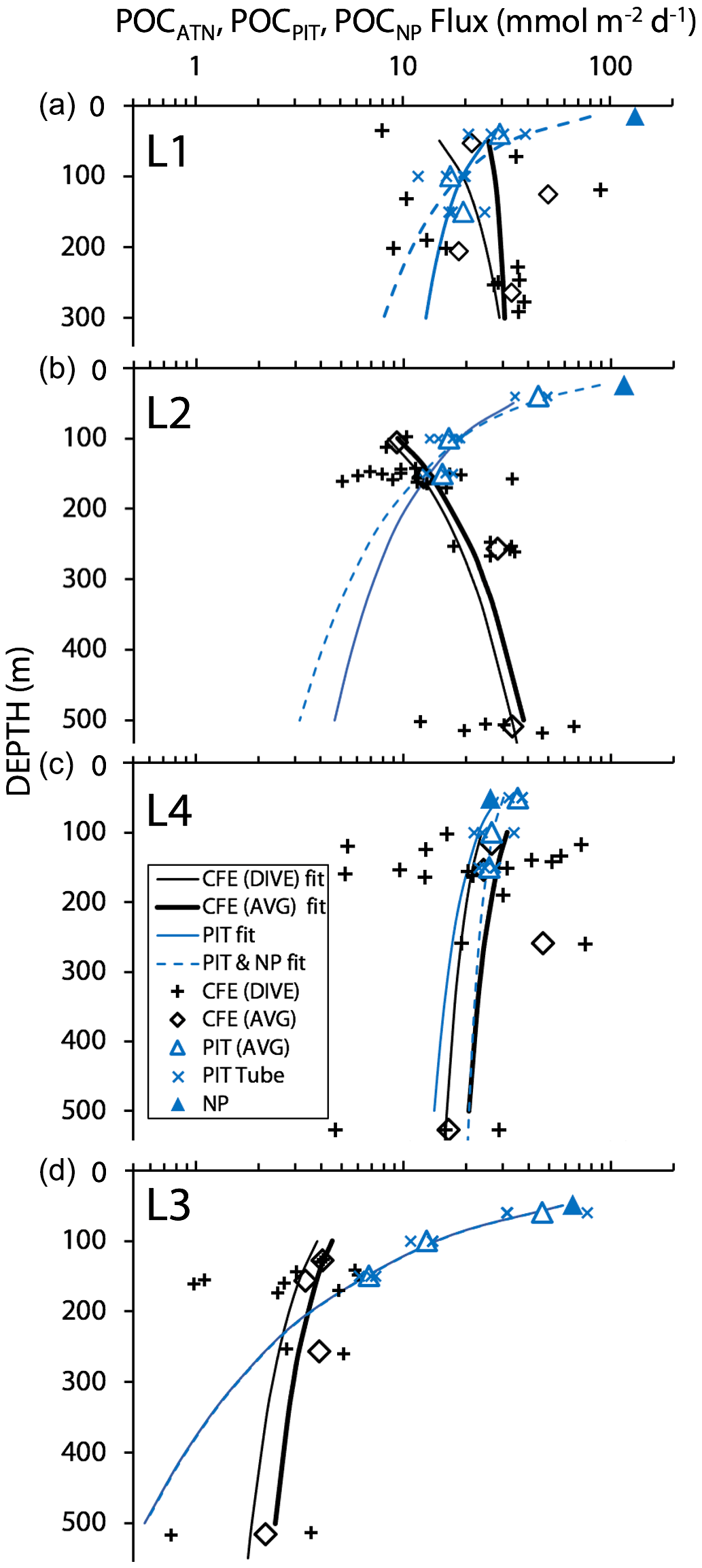
Figure 16Comparison of CFE, PIT and NP POC flux estimates at the three filament locations L1, L2 and L4 and at L3 in transitional waters. The thin and heavy black lines are the “Martin” curve fit for individual CFE dives (data shown by +) and for pooled time-averaged data (diamonds), respectively. The solid and dashed blue lines denote Martin curves based on fits to PIT (particle interceptor trap) results and to combined PIT result and new production (NP, solid triangle) data. At L1, the blue curves underestimate fluxes at 250 m by a factor of 2. At L2, blue curves underestimate flux by a factor of 6 at 500 m. At L4, there was close agreement among methods. At L3 (with sparse data), fluxes were underestimated by a factor of ∼2 at 500 m. POCATN flux was calculated from volume attenuance flux (VAF, mATN cm2 cm−2 d−1), where one VAF unit = 1 mmol C m−2 d−1 (Bourne et al., 2019). PIT and new-production-based carbon flux (mmol C m−2 d−1) are from Kranz et al. (2020). The larger scatter in individual CFE dive data compared to PIT data is attributed to the fact that results are representative of 5 h of observations vs. 3–4 d.
Total POCATN flux increased with depth at L2 from 12.4 mmol C m−2 d−1 at 150 m to 28.3 mmol C m−2 d−1 by 250 m and to 38 mmol C m−2 d−1 by 500 m (Fig. 16). At L3, in transitional waters outside the filament, POCATN flux varied with depth from 3.8 mmol C m−2 d−1 at 150 m to 3.9 mmol C m−2 d−1 at 250 m and 2.4 mmol C m−2 d−1 by 500 m. At L4, flux at 150 m averaged 25 mmol C m−2 d−1 (range 5–72 mmol C m−2 d−1). Interestingly, none of the locations showed a strong decrease in flux with depth as one would expect based on the traditional Martin curve (Fig. 16). POCATN flux at L1 and L2 increased with depth with Martin b values (95 % confidence interval in parentheses) of +0.37 (±0.59) and +0.85 (±0.31), respectively. Trends at L3 and L4 yielded b values of −0.45 (± 0.70) and −0.24 (± 0.68), indicating flux trends that slowly decrease with depth, trends similar to those reported by Bishop et al. (2016).
3.5 Water column POC
Transmissometer beam attenuation coefficient is a strong optical proxy for POC in the upper kilometre of the water column (Bishop, 1999; Bishop and Wood, 2008; Boss et al., 2015). Between 41 % and 89 % of this signal is typically due to beam interaction with relatively small, slowly sinking particles (Chung et al., 1996; Bishop, 1999). Surface layer transmissometer-derived POC ranged from a high of 35 µM at L1 to a low of 2 µM at L4 (Figs. 11 and 12, Table 2).
The integrated standing stock of POC in the water column was highest closest shore at L1 and progressively dropped with distance offshore (and time) in the filament (Fig. 10). At L1, where the sea floor was at 450 m, relatively high POC levels (averaging ∼ 1 µM) were detected in the 300 to 450 m interval, indicative of resuspended particles forming a bottom nepheloid layer. It is important to note that CFEs did not sample in the nepheloid layer.
4.1 Circulation
When considering carbon export dynamics, especially in regions with strong current systems, it is essential to understand the vertical profile in the context of the physical environment. As mentioned previously, by June 20–25, a depression in sea surface height (SSH) roughly 100 km in diameter had developed about 200 km off the coast. Such a SSH depression indicates the formation of a cyclonic eddy as Ekman transport would yield a net transport out of the centre to the edge of the eddy as waters rotate clockwise around the centre. As CFEs are Lagrangian, they drift with currents at depth during deployments, and their positions over time can be used to infer current velocity (Sect. 3.2). The CFE trajectories from dives to 150 and 250 m all reinforce such anticlockwise motion, consistent with ADCP data (Figs. 4 and 9). Waters at L1, located ∼ 20 km from the coast, were strongly influenced by tidal motion but overall flowed offshore to the west. At L2, the water was flowing quickly to the west-northwest. As this westward-flowing water encountered offshore water flowing eastward, a cyclonic eddy formed, with anticyclonic eddies forming to the north and south. L3 was located outside of a developing cyclonic eddy, with water moving quickly to the southeast. L4 was in slow-moving waters close to the centre of the eddy. These large-scale circulation patterns, with consistent directionality of water flow traced by CFEs at all depths, have implications for the flux profiles as discussed in depth below.
4.2 Comparison with other studies
Siegel et al. (2014) estimated carbon fluxes carried by algal aggregates and zooplankton faecal matter at the base of the euphotic zone from a food web model driven by satellite observations including SST, chlorophyll a, net primary productivity, and particle size for monthly climatological conditions. The Siegel et al. (2014) climatological flux for June in our region is shown in Fig. 17a. Recognizing the spatial coarseness of the 1 × 1∘ gridded data set of Siegel et al. (2014), the model predicts a base of euphotic zone flux of about 20 mmol C m−2 d−1 near-shore, with progressively lower fluxes going offshore to values of around 5 mmol C m−2 d−1 at offshore L3. In order to compare CFE flux results at 250 m, these modelled euphotic zone export fluxes were extrapolated to 250 m using Eq. (1) and the Martin b value of −0.83 reported by Martin et al. (1987) for the VERTEX 1 site (Fig. 2). POCATN fluxes at 250 m are plotted in the figure and are higher in all cases except in the transitional waters at L3. The point of this comparison is that filaments appear to make a disproportionately large contribution to carbon transfer to deeper waters and that such filaments need to be included in models.
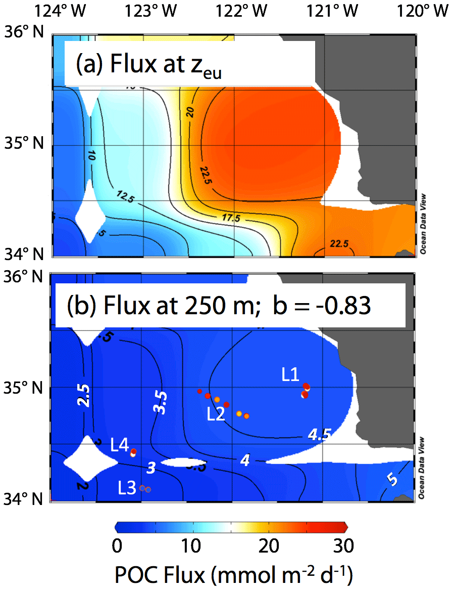
Figure 17(a) Euphotic zone carbon export for climatological averaged June from Siegel et al. (2014). (b) Fluxes calculated for 250 m using Eq. (1) and the b value from VERTEX I (−0.83; Martin et al., 1987). The euphotic zone depth (zeu) used for the calculation was June climatology from NASA VIIRS. Also shown using the same colour scale are POCATN flux values near 250 m. The CFE fluxes are far higher than model predictions at depth at all locations except L3.
One of the closest observations in terms of distance from coast, season, and span of the water column is the VERTEX-1 (V-1; Martin et al., 1987). Martin's station V-1, occupied in June 1984 in intense-upwelling and high-chlorophyll conditions, was located off the coast of Point Sur approximately 100 km north of L2 (Fig. 2). VERTEX deployed surface-tethered particle interceptor (PIT) sediment traps from 50 to 2000 m, similar to those deployed during CCE-LTER. V-1 fluxes at 50 and 100 m were 25 and 19.6 mmol C m−2 d−1. At L1, our CFE fluxes at 50 and 125 m were 21 and 50 mmol C m−2 d−1, respectively. Although V-1 fluxes were similar to our results, the profiles in deeper waters diverged. Flux at L1 was nearly constant or slowly increasing with depth and the flux at L2 increased with depth; in contrast, V-1 data decreased strongly. The comparison with VERTEX results is justified since Point Sur has been identified as an area of frequent filament development (Abbot and Barksdale, 1991; Gangopadhyay et al., 2011); furthermore, chlorophyll fields mapped using the NASA Coastal Zone Colour Scanner in June 1984, although few, confirm a filament structure near V-1 at the time of sampling (Fig. A7).
There are two candidate explanations for why V-1 results and our data taken in similar conditions display such different behaviours. First, L1 was located over a wide 500 m deep “shelf” and L2 offshore was down-current of this feature, whereas V-1, in 3 km deep water, was offshore of a much narrower shelf (Fig. 2a). When high export occurs over a broad shelf, particles can accumulate in a fluff layer near the bottom and be resuspended in a nepheloid layer. Such a layer can clearly be seen at L1 in both transmissometer-derived POC and in water turbidity (Fig. 11), and thus there is a potential source of particles to offshore waters.
The second possible explanation is that many of the > 1000 µm sized aggregates seen in CFE imagery would be excluded from surface-tethered baffled PIT traps due to “baffle bounce” (Bishop et al., 2016), observed when currents relative to the trap are faster than 0.02 m s−1. Stated another way, the size scale of the aggregates relative to the centimetre-scale baffle opening on traps, coupled with a near-horizontal encounter with the trap opening, would cause aggregates to bounce back into the flow and thus not be sampled. This was observed using surface-tethered OSR instruments during quiescent conditions in the Santa Cruz Basin (Bishop et al., 2016). In our observations of the relative behaviour of PITs and CFEs, relative current speeds across the PITs were generally faster than this threshold. While smaller particles at L2 did attenuate with depth, aggregate fluxes increased (Fig. 15a); thus there is support for this hypothesis.
Surface-drogued PIT traps were deployed at 50, 100, and 150 m during the CCE-LTER study (Kranz et al., 2020). At 150 m at L1, L2, and L4, trap-measured flux and CFE-derived fluxes (Fig. 16) were in relatively close agreement. At L3 in transitional waters, PIT trap fluxes at 150 m were 2 times higher than CFE results; however, the strong surface current regime encountered there rapidly separated the two observing systems spatially. Based on the reasonable agreement of results, the second candidate explanation is disfavoured.
In Sect. 2.2.4 we investigated sources of error. We concluded that the 9 % uncertainty in the VAF : POC flux relationship and its assumed constancy with depth are not a factor in the interpretations that follow. The contribution of counting errors to POCATN flux in the 1000–10000 µm size category is small at locations L1, L2, and L4 and does not change our main conclusions below; errors in POCATN flux are illustrated in Fig. A5b.
If trap fluxes from 50, 100, and 150 m are fit with a Martin function, does the extrapolated curve adequately match POCATN fluxes deeper in the water column? Figure 16 depicts POCPIT and POCPIT + POCNP fluxes extrapolated to depth using the Martin regression applied to 50–150 m results (data in Table 4). At L1, L2, L4, and L3 Martin b values (95 % confidence interval in parentheses) were −0.37 (± 0.27), −0.86 (± 0.22), −0.30 (± 0.19), and −2.01 (± 0.51), respectively; three of four regressions are significantly different (at > 95 % confidence) from Martin curves. Fits combining POCPIT and POCNP fluxes yield b values of −0.78 (± 0.34), −1.11 (± 0.26), −0.16 (± 0.26), and −2.02 (± 0.41) for L1, L2, L4, and L3 (respectively). In this case, L3 and L4 remain significantly different from classic Martin curves. At 300 m (L1) and at 500 m (L2 and L3), POCPIT Martin extrapolated fluxes would fall lower than CFE fluxes by factors of 2.1, 6.8, and 4.9. Only at L4 did fluxes agree well. The first takeaway is that Martin b factors are rarely “classic” and often are substantially lower than expected. The second takeaway is that the mismatch (POCPIT extrapolated vs. POCATN observed) indicates that fundamental processes contributing to the flux profile are not accounted for by the Martin relationship in deeper waters.
Considering the two candidate explanations above, we hypothesize that some ecological or physical process linked to a wide–shallow continental margin environment leads to more efficient transfer of POC through the water column in the CCE_LTER study case. More work on the intercomparison of PIT traps and CFEs, particularly particle classes sampled, would resolve any sampling bias issues. While mesoscale (4 km) chlorophyll variability (Sect. 3.1; Fig. 5b) at L2 was small, there is no insight regarding the variability of particle flux from these observations.
4.3 Mechanisms for non-classic Martin behaviour
In the CCE–LTER process study reported here, we do not observe total POCATN flux attenuating with depth deeper than 100 m at any of our locations. At two locations we see flux near constant or increasing with depth. At other locations we observe flux decreases with depth at a rate slower than predicted by the Martin formulation. We explore reasons why the flux profile from the coastal station VERTEX-1 (Martin et al., 1987, Fig. 1), which follows the classic curve, differs from results of this study. In the following discussion, we use the term “non-classic” to represent such behaviour.
Figure 18 depicts four mechanisms which could explain why particle flux profiles may diverge from traditional Martin-like behaviour: (1) non-steady-state flux and/or remineralization (Giering et al., 2017), (2) inputs from migratory organisms at depth (Turner, 2015; Bishop et al., 2016), (3) physical subduction of surface material along isopycnal surfaces (Omand et al., 2015; Stukel et al., 2018), and (4) lateral horizontal transport of resuspended particles from the continental margin followed by aggregation and sinking (Pak et al., 1980; McPhee-Shaw et al., 2004; Chase et al., 2007; Alonso-González et al., 2009).
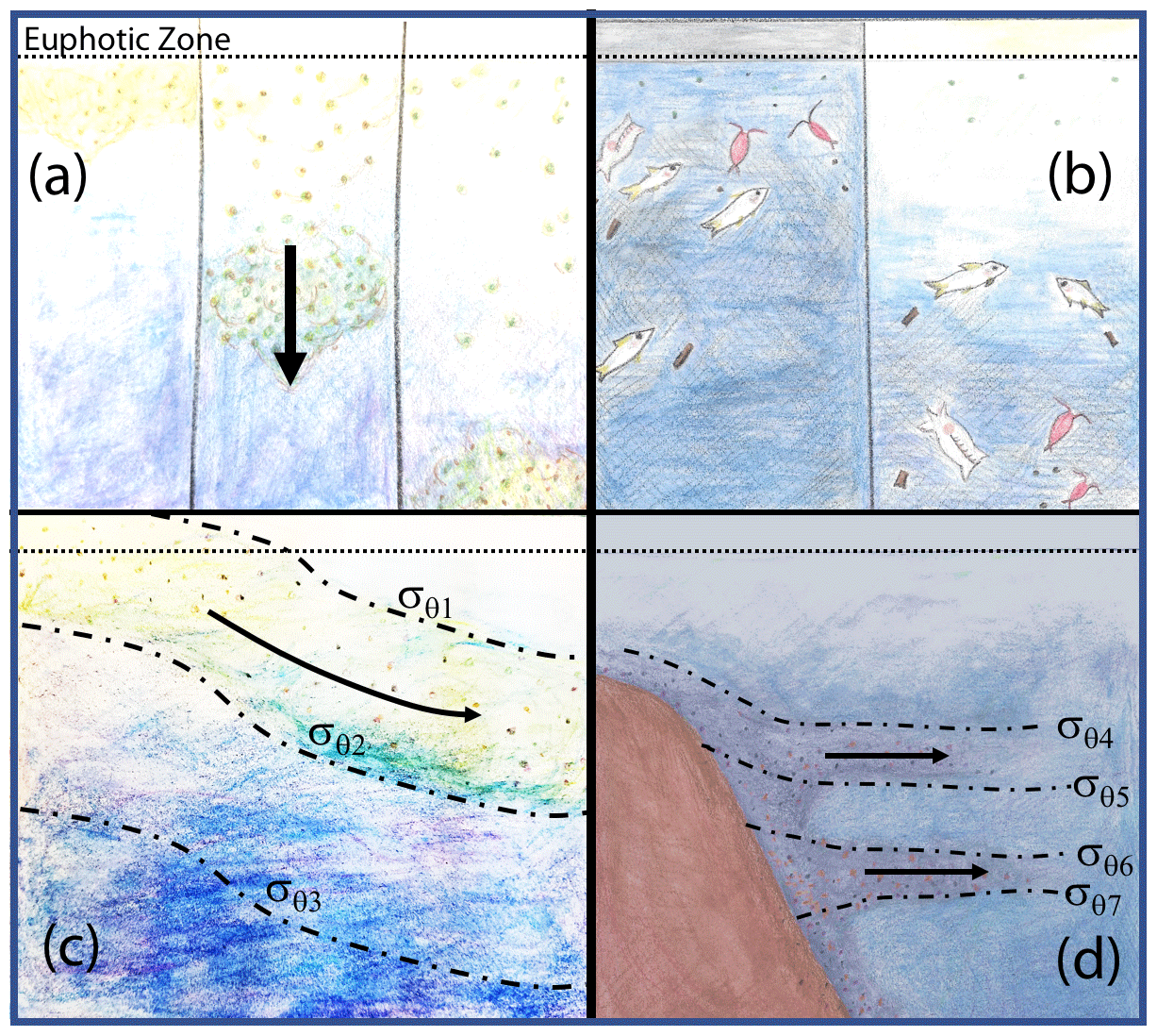
Figure 18Four mechanisms that can lead to non-classical particle flux profiles. (a) Temporal delay (Giering et al., 2017), (b) vertical migration (Turner, 2015; Bishop et al., 2016), (c) physical subduction (Omand et al., 2015; Stukel et al., 2018), and (d) sediment resuspension and lateral advection (Alonso-González et al., 2009; Pak et al., 1980; McPhee-Shaw et al., 2004; Chase et al., 2007).
4.3.1 (M1) non-steady-state flux
The Martin et al. (1987) formula assumes a steady state over the several days required for particles to transit from the base of the euphotic zone to mesopelagic depths (500 m in our case); however, CCE-LTER sampled a rapidly evolving system. Upwelled coastal water can spawn productive filaments and eddies that persist less than a month. Giering et al. (2017) describe cases, especially associated with bloom scenarios, where the water column may not be in steady state. Figure 19 depicts two such scenarios in which export and remineralization are time varying in a way that leads to an apparent non-varying flux with depth or to an increased flux with depth.

Figure 19Scenarios which could lead to flux not systematically decreasing with depth. (a) Depicts constant flux at the reference depth, with time variant values of the Martin b parameter. (b) Depicts a scenario with constant Martin b, but decreasing flux at the reference depth over time (after Giering et al., 2017). Red marks indicate sampling points in both figures, illustrating how temporal delay could lead to observations of increasing flux with depth.
Non-steady-state blooms and time-variable changes of the b factor can lead to inverted flux profiles as there is a temporal lag between peak export from the surface layer and the arrival of particles at depth (Figs. 18a and 19). One indicator of a temporal delay scenario would be finding ungrazed intact phytoplankton from a prior bloom at depth. CTD chlorophyll fluorescence data, however, show no evidence of sinking ungrazed phytoplankton (Figs. 11 and 12). Furthermore, there is also no major trend of flux either increasing or decreasing with time at L2 (Fig. 5). That particle flux at 250 m L4 was 2.5 times higher than measured new production provides some support for the non-steady-state flux mechanism at L4.
4.3.2 (M2) efficiency of grazing community and active transport
Zooplankton are highly important to POC export as their faecal pellets or feeding webs package smaller non-sinking phytoplankton and particles; however, flux due to zooplankton-produced faecal pellets and aggregates is highly dependent upon the zooplankton community present (Turner, 2015; Bishop et al., 1986; Boyd et al., 2019). Furthermore, the community of phytoplankton that develop seasonally and during the course of a bloom can have a great impact on how surface material is exported to the mesopelagic.
High levels of production and biomass do not necessarily imply high export (Bishop et al., 2004, 2016; Lam and Bishop, 2007). In a multi-cruise study in the Santa Cruz Basin south of the CCE-LTER study area, Bishop et al. (2016) found that the highest export levels coincided with the lowest levels of surface chlorophyll. None of the POCATN flux profiles from the cruises (January 2013, March 2013 and May 2012) were traditional Martin curves. High levels of productivity combined with efficient grazing and weak remineralization likely combined to create the conditions of very high flux (but low surface chlorophyll) observed in January 2013 (Bishop et al., 2016).
Vertical migrators can also transport material to depth (Fig. 18b). Diel vertical migrators such as euphausiids, salps, and copepods consume material at the surface during feeding times and then can excrete material when they retreat to depth (Steinberg et al., 2008). Fish can also transport consumed material to depths far below the euphotic zone.
Some heterotrophs produce faecal material that is much more efficient at being exported from the euphotic zone. Organisms such as krill and fish produce large dense faecal pellets which sink very efficiently. At L1, the near-constant flux with depth was due in large part to fast-sinking anchovy pellets. It has been reported that both copepod (Smetacek, 1980; Krause, 1981; Bishop et al., 1986; Bathmann et al., 1987; González et al., 2000) and protozoan (González, 1992; Beaumont et al., 2002) pellets do not have high transfer efficiency on sinking from the euphotic zone. González et al. (2000) found that only 0.1 %–2.5 % of copepod faecal pellets in the upper 100 m Humboldt current reached sediment traps at 300 m. The fast recycling of copepod faecal pellets in the surface has been attributed primarily to coprophagy (Beaumont et al., 2002; Smetacek, 1980). Evidence suggests that the fast recycling of zooplankton pellets in the epipelagic is due to the activities of other zooplankton (Turner, 2015, and references therein). There are a number of zooplankton known to eat faeces (coprophagy) including radiolarians (Gowing, 1989), tunicates (Pomeroy et al., 1984), and copepods (Sasaki et al., 1988).
At L2 at 150 m, 200–400 µm sized ovoid pellets were very abundant and were fast sinking. The ovoid pellet number flux at 150 m was 150 000 m−2 d−1; however, by 500 m, the pellets' flux was reduced by a factor of 20 (Fig. 8a). These trends were confirmed and calibrated by manual particle counts (Connors et al., 2018). The membrane-bound small ovoid pellets were olive coloured (Fig. 6g) and shown in SEM imagery to be full of diatom frustules and fragments as were the anchovy pellets at L1 (Fig. A6). At L3 and L4, the pellet flux decreased from 100 to 500 m by factors of 8 and 5, respectively; at L1 the decrease was 2.5-fold between 50 and 250 m (Fig. 8c).
At L2, as the ovoid pellets decreased with depth, the concentration of aggregates, many of which closely resemble discarded larvacean houses, increased to dominate POCATN flux (Fig. 15b). Larvaceans produce fine mucous feeding webs that concentrate and ingest particles from 0.2 to 30 µm in diameter (Gorsky and Fenaux, 1998). Typically, a larvacean feeds on only a fraction of the material in its web before it discards it due to clogging (Berline et al., 2011); furthermore, some larvaceans create and discard up to 26 feeding webs a day (Sato et al., 2001). They therefore can be major contributors to carbon flux. Larvaceans are found throughout the upper 1000 m (Stemmann et al., 2008), and they are often the most abundant mesozooplankton after copepods (Gorsky and Fenaux, 1998). Larvaceans with intact feeding structures are difficult to study as they are fragile and therefore difficult to capture in plankton nets (Berline et al., 2011; Silver et al., 1998). The larvaceans without houses are captured in net tows; however, newly reported results from Zooglider, an autonomous buoyancy-driven glider with interfaced zooplankton imaging system, showed order-of-magnitude higher abundances of larvaceans compared to simultaneous MOCNESS collections during operations in the vicinity of the La Jolla canyon in March 2019 (Whitmore et al., 2019). It is clear that the full impacts on flux by migratory communities and their modification of sinking particle flux is, as of yet, only partly realized.
Vertical migration likely does contribute export to depth. At L2, we did see evidence of migration to 250 m in preliminary biomass profiles from MOCNESS tows (Mark Ohman, personal communication, July 2020) and in ADCP scattering intensity records. However, the increase in flux with depth cannot solely be explained through transport of material from the surface to depth through vertical migration. For one, vertically migrating crustacean species in the CCE have a gut turnover time of about 30 min; thus in the 1–2 h to swim to depth only 50 % or 25 % of excreted material would be delivered to 250 m, where we see increased flux. The aggregates at depth are clearly not aggregations of faecal pellets. This does not rule out that vertical migrators were important, as gelatinous organisms such as larvaceans and salps have been known to migrate daily. A quantitative analysis of the CCE–LTER MOCNESS speciation and of multifrequency fisheries echo sounder data would help resolve these questions but has yet to be performed.
Does active transport explain the flux increase at L2? At L2, Kranz et al. (2020) report POCNP export flux of 101.6 ± 44.0 mmol C m−2 d−1, in close agreement with our calculated export flux of ∼ 120 mmol C m−2 d−1 for the 9 d period between studies at L2a and L4 (Sect. 2.4). Sinking particles are consumed by particle grazers, and assimilation efficiency can vary by species and food substrate. Previous work has reported that salps have a 61 % assimilation efficiency for carbon (Madin and Purcell, 1992). If exported particles were processed using this efficiency, and if all particles were consumed by vertically migrating organisms and excreted at depth, there would be a flux of 48 mmol C m−2 d−1. The same calculation assuming an assimilation efficiency of 90 % would add ∼ 12 mmol C m−2 d−1 at depth. Flux at 500 m at L2 was 38 mmol C m−2 d−1, which would require dominant migratory inputs. While vertical migrators are likely important contributors to flux, their activities may not fully explain the depth-increasing-flux profiles observed at L2. It is clear that the flux carried by aggregates at depth cannot form from the coprophagy of sinking faecal pellets.
4.3.3 (M3) physical subduction
In most regimes, export of particulate organic carbon (POC) to depth is primarily attributed to sinking particles; however, in dynamic regimes sub-mesoscale eddy-driven flux may be responsible for transporting a significant percentage of living phytoplankton along isopycnal surfaces to depth (Omand et al., 2015; Fig. 18c). The filament we followed produced a cyclonic eddy with divergent surface water flows, which would have led to upwelling, not downwelling. While subduction of ungrazed phytoplankton may also occur at fronts, there is no evidence to support a subduction process connecting the surface layer to 250 m at L2 as chlorophyll fluorescence profiles (Fig. 11) show minimal presence of phytoplankton material deeper than 100 m. Spatial transects across the filament furthermore showed little evidence of fluorescent particles deeper than the σθ=26.0 kg m−3 isopycnal at 100 m (Fig. 12). Our findings are consistent with those of Stukel et al. (2018), who found in targeted study of fronts in the CCE region that subducted particles were completely remineralized by 150 m. Eddy-driven subduction and frontal subduction processes do not play a role in fluxes seen in our data.
4.3.4 (M4) lateral advection
Turbulent currents interacting with continental shelf and upper slope sediments can pick and transport sediment and fluff layer material offshore along isopycnals (Fig. 19d). Along the flow path filter feeding organisms can consume the particles and produce sinking material, adding to vertical flux and thus increasing POC flux at depth. The California Current eastern boundary regime is typical of such conditions. Intermediate nepheloid layers found at several hundred metres depth off the coast of Oregon were tracked to a continental shelf sediment origin (Pak et al., 1980). Similar layers have been observed between 70 and 150 m on the outer continental shelf off northern California (McPhee-Shaw et al., 2004). In a box model study of the Canary Current region, Alonso-González et al. (2009) calculated that lateral suspended POC fluxes of continental shelf origin were up to 3 orders of magnitude greater than vertical fluxes. Their results suggest that laterally sourced POC could be a significant part of the mesopelagic carbon current budget in their study area. If their model is applicable to other eastern boundary current regimes, then laterally sourced POC transport may play a crucial role in global carbon cycle.
Kelly et al. (2018) found an inverse relationship with higher e-ratios (the ratio of export at the euphotic zone base to net primary productivity) in offshore regions and lower e-ratios in the more productive coastal regions over five CCE cruises. Furthermore, a strong correlation between sea surface temperature and export was found, which they determined not to be causal but rather an effect of lateral advection bringing upwelled cold productive waters offshore.
Observed nepheloid layers near L1 might indicate that lateral transport could be a possible factor explaining flux increase with depth at L2 in our study. Support for this comes from the finding of strong offshore currents at L2 (Fig. 9b and c). During the first 2 d of the CFE deployment, transports were to the west–northwest, with velocities averaging 0.2 m s−1 between 100 and 300 m. CFE trajectories during 500 m dives indicate that deeper water was also moving in the same direction (Fig. 9). The offshore flowing currents, if carrying a high concentration of non-sinking POC derived from the shallow continental margin near L1, could supply a substrate for particle gazers at depth. Alternatively, large aggregates sourced shallow in the water column between L1 and L2 could be present in deeper waters at L2a and thus explain the apparent increase in flux with depth at L2.
On the other hand, several points of evidence argue against lateral transport and repackaging of nepheloid or fluff layer material as contributing to POCATN flux at L2. First, the nepheloid layer is seen at L1 in the 300–450 m interval (average POC = 1.4 µM; Fig. 11), and a similar intermediate nepheloid layer found at L2a between 50 and 250 m occurs in waters of very different density; the nepheloid layer at L1 occurs in waters with a σθ range of 26.7–26.92 kg m−3, whereas the L2a layer is found in waters with σθ ranging from 26.1–26.7 kg m−3; the feature is absent at L2b (Fig. 12). Secondly, UVP5-hd data show that the nepheloid layer at L1 is dominated by smaller particles and not > 1000 µm sized aggregates. In fact, in the 100–300 m depth interval there were fewer > 1000 µm aggregates at L1 than at L2, and aggregates had identical concentrations below 300 m (Fig. 20). This rules out a direct connection involving the advection of large aggregates or resuspended small particles from L1.
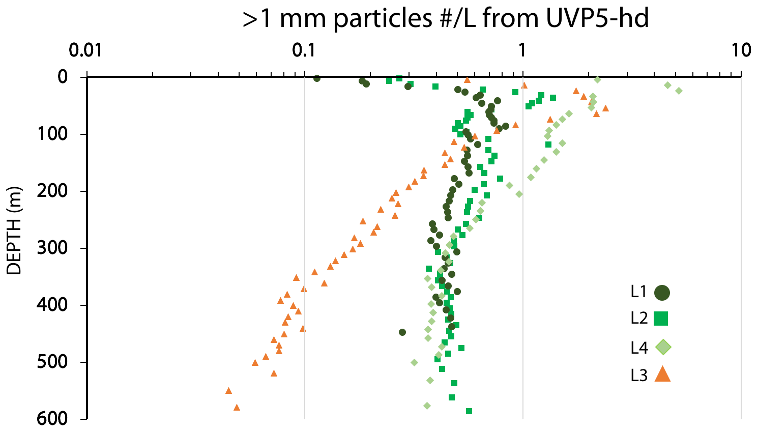
Figure 20Mean non-living particle number concentrations for >1.024 mm sized aggregates from UVP5-hd profiles. Averages were from pooled CTD casts at filament locations L1, L2, and L4 and in transitional waters outside of the filament at L3. Aggregate numbers were more abundant in the waters beneath the filament than in transitional waters below 100 m, consistent with CFE observations.
4.3.5 Recap of flux mechanisms
We are left with a puzzle. All small particle classes smaller than 400 µm exhibit a decrease with depth at all locations consistent with a single origin within the euphotic zone and progressive particle remineralization during sinking. At the same time > 1000 µm aggregate fluxes either increase with depth (L1 and L2) or slowly decrease (L3 and L4); the increased flux cannot be supplied by biologically mediated consumption and repackaging of the smaller-sized sinking particles because the fluxes of < 1000 µm particles are too low. Our strongest candidate mechanism to explain the > 1000 µm POCATN flux profile at L1 and L2 is active transport (M2) or some related process transforming the DOC pool to POC flux at depth. Due to the strong decline in measured new production at L4, non-steady-state export (M1) may have been an additional contributing factor at L4. The subduction (M3) and lateral transport (M4) mechanisms are disfavoured.
4.4 Anchovy faecal pellets: enhancement of carbon and phosphorous transfer efficiency
As noted in Sect. 3.3 above, anchovy pellets were major contributors to flux at L1. Previous research has found that these large and dense faecal pellets sink at 750 m d−1 and are very efficient transporters of organic matter to the deeper ocean (Saba and Steinberg, 2012). SEM imagery of anchovy pellets sampled by CFE-Cal showed that the anchovies were primarily grazing on diatoms (Fig. A6). Another indication of the efficiency of transport comes from the analysis of phosphorus and organic carbon in CFE-Cal samples (Bourne et al., 2019). Anchovy-pellet-dominated samples collected using the CFE-Cal at L1 had an organic carbon-to-phosphorus (C : P) ratio of 60 : 1, much lower than the typical 300 : 1 ratio found in other samples; P is known to be lost rapidly relative to organic carbon from sinking particles (Collier and Edmond, 1984). Not only are anchovies primary grazers and thus potentially strong contributors to flux, they also appear to be enhancing the vertical transfer of phosphorus relative to carbon to the deep sea.
Coastal upwelling regions are disproportionately productive relative to their total surface area due to high levels of available nutrients. Four Lagrangian carbon flux explorers (CFEs) were deployed a total of 24 times during the 2 June through 1 July 2017 California Current Ecosystem – LTER process study of a dynamic filament of productive water as it moved from the coast to the open ocean.
The CFEs provided an unparalleled view of particle flux and particle flux size distribution (30 µm to centimetre scale) within that system. In all environments, flux was dominated by particles > 200 µm in size. At L1, > 1000 µm anchovy pellets dominated. At L2, 200–400 µm sized olive-coloured ovoid pellets contributed on average ∼ 50 % of the flux and at times accounted for 100 % of the flux at 100 to 150 m. At all locations, > 1000 µm sized amorphous aggregates dominated flux at depths greater than 150 m.
We found during the CCE-LTER study that flux does not decrease with depth following a typical Martin power-law () relationship in many instances. Extrapolating POC flux from the euphotic zone to depth using the classic Martin curve in such productive regions strongly underestimates flux. Interestingly, flux profiles for particle classes smaller than 400 µm always had negative b factors which were more closely in agreement with the classic Martin fit.
In this study of particle fluxes from 100 to 500 m, the highest flux was found at L1, where surface chlorophyll initially exceeded > 10 mg m3. However, the magnitude of flux did not always correlate with surface chlorophyll. L4 had nearly the same flux, though surface chlorophyll was 50 times lower than at L1. We confirm the Bishop et al. (2016) conclusion that surface chlorophyll in the California coastal environment is a poor indicator of flux at depth. The efficiency of export was clearly affected by trophic structure as evidenced by the dominant particles contributing most vertical carbon flux. At L1, flux was very efficient as anchovies directly grazed on primary producers and produced dense phosphorus-rich, fast sinking pellets. At L2, though copepods were ubiquitously higher in the water column and their faecal pellets were an important contributor to flux at 150 m, the contribution had largely disappeared by 250 m depth. At all locations the ovoid faecal pellet fluxes decreased as expected with increasing depth (Fig. 8) consistent with their production in or just below the euphotic zone and progressive loss with depth. Their pellets were not significant contributors to carbon flux deeper in the mesopelagic layer.
At L2, and to some extent at L1, there was a shift from faecal pellets near the surface to large aggregates at depth. At L3 and L4, large aggregates dominated POC flux at all depths. These aggregates resembled discarded larvacean feeding webs, although they may have other origins. There was no direct evidence that westward-moving currents laterally transported waters with POC or aggregates from the continental margin.
The flux profiles observed at most locations were unlike the classic Martin curve. As mentioned previously, the VERTEX-1 site in the classic Martin et al. (1987) study was located 100 km north of our L1 and L2 study areas and took place under similar conditions (including active upwelling and the presence of a filament). This study has found high fluxes and transfer efficiencies through the mesopelagic zone, similar to observations in the nearby Santa Cruz Basin (Bishop et al., 2016). Both regions are adjacent to wide shallow shelves, whereas the observations of Martin et al. (1987) took place near a narrow shelf (Fig. 2). Shelf width is implicated in the supply of bioavailable iron to surface water phytoplankton communities (Johnson et al., 1999; Chase et al., 2007; Lam et al., 2006), with narrow continental shelf regimes being more iron limited. We use the analogy to iron supply to raise the question of whether flux profile differences are the result of intrinsic differences in the zooplankton–fish community composition, grazing and migratory behaviour, or food web structure in offshore waters near narrow vs. wide continental shelves.
At the time of writing, we are unable to fully explain the particle flux increase at L2 between 100 and 500 m, and we have not closed the story of the origins of the aggregates that dominate flux in all waters deeper than 150 m. This study shows that there are many new questions pertaining to filament dynamics and POC flux.
Fluxes made with surface-drogued PIT traps were generally in agreement with CFE fluxes near 100 and 150 m, suggesting that discrimination against > 1500 µm aggregates as proposed by Bishop et al. (2016) may not be as important in the strong upwelling and wave conditions encountered during the CCE-LTER study; however, extrapolation of 50 to 150 m PIT fluxes to depth using Martin fits led to significant (factors of 3 to 7) underestimation of flux at the deepest depth horizon sampled by CFEs, again raising the question of how the deep aggregate populations and fluxes are achieved.
Unlike sample-collecting devices (including CTD–rosettes, drifters, surface-drogued sediment traps, and CFE-Cals) that must be ship-deployed, CFEs have a mission capability of 8 months of hourly operations (or 16 months at 2 h) and have been deployed for missions of up to 40 d without compromise; the CFEs have been proven in a wide range of sea states and to depths of 1000 m (Bishop et al., 2016). Due to the complexities of particle size distribution and particle class measurement, which is not yet implemented on the CFE, all deployments have been tended by ships to date. The framework provided by the CCE-LTER process study provided an opportunity to advance towards full CFE autonomy while supporting science. Our hybrid size distribution analysis scheme provided key insights that are an important step towards fully autonomous operations in the global ocean. Both methods 1 and 3 (after modification) would be possible to run on the CFE during deployment.
In coastal regions, carbon export needs to be understood both laterally and vertically. A future expanded scope of autonomous observations during process studies and surveys would provide a 3D view of mechanisms dictating export in these regions and inform the new class of eddy-resolving simulations of biogeochemical processes in the California Current System such as recently described by Deutsch et al. (2021).
Table A1Comparison of pellet and aggregate flues from manual enumeration and from particle analysis method 3.
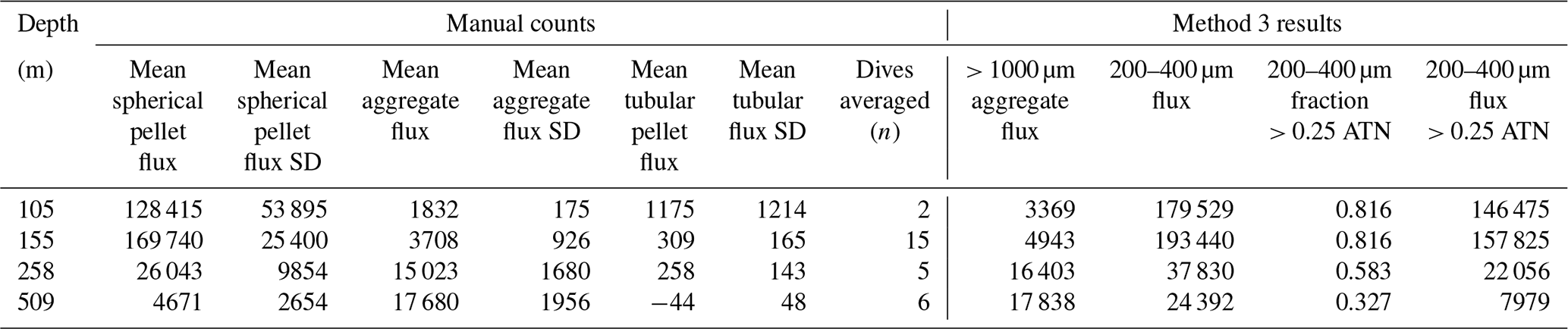
Flux units no. m−2 d−1. Tubular pellet data represent numbers of individually occurring > 1000 µm long euphausiid pellets. These data are plotted in Fig. 8.
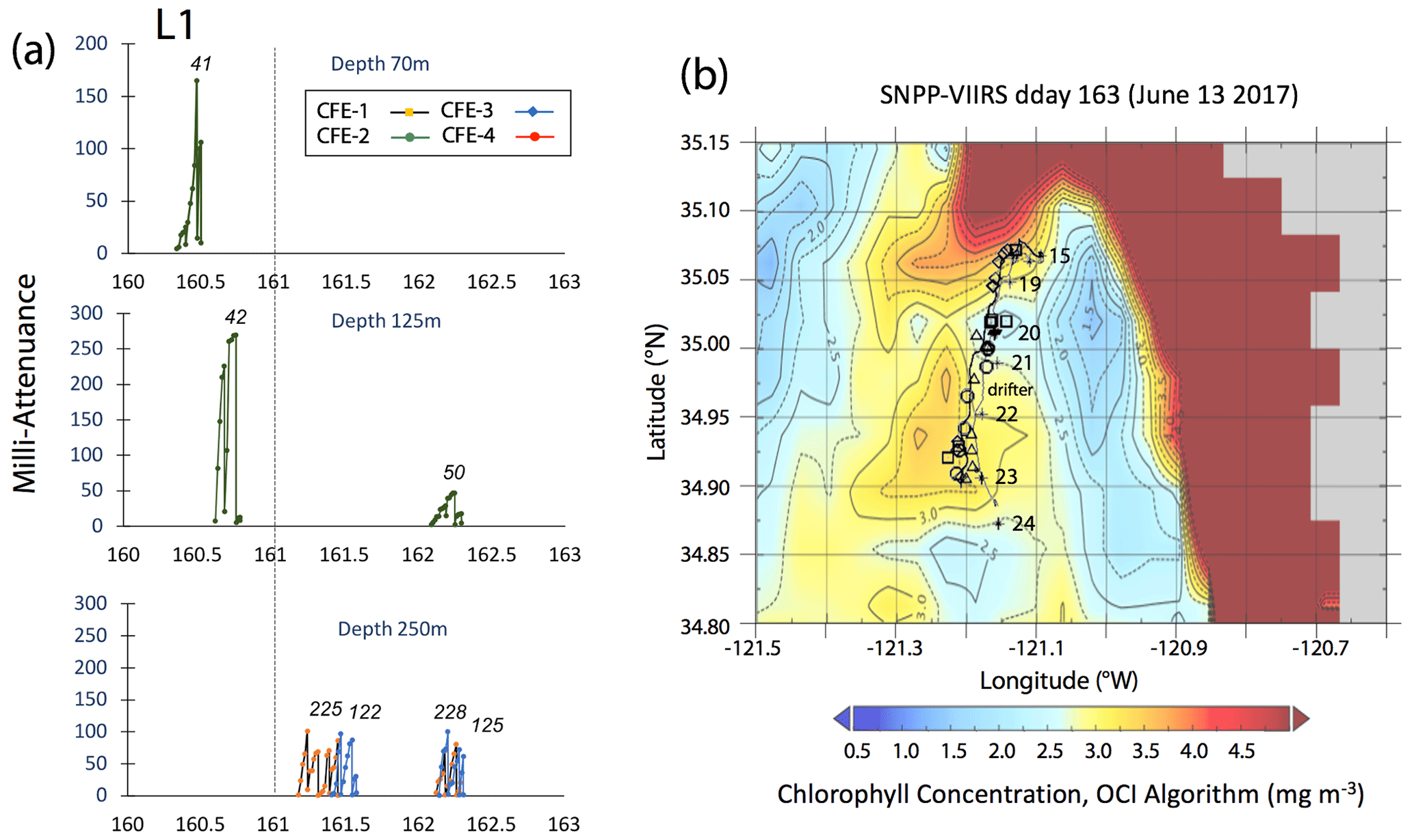
Figure A1(a) Raw attenuance time series for CFEs deployed at L1 (300 m data not shown). See Fig. 2 for deployment context. Italicized numbers are CFE dive numbers. (b) Map showing deployment and trajectories of CFEs, CTD station locations, and tracks of the productivity drifter and sediment trap array during the intensive studies at L1. The overlay is the SNPP VIIRS chlorophyll field for 13 June 2017. CTD cast numbers are shown on the plot.
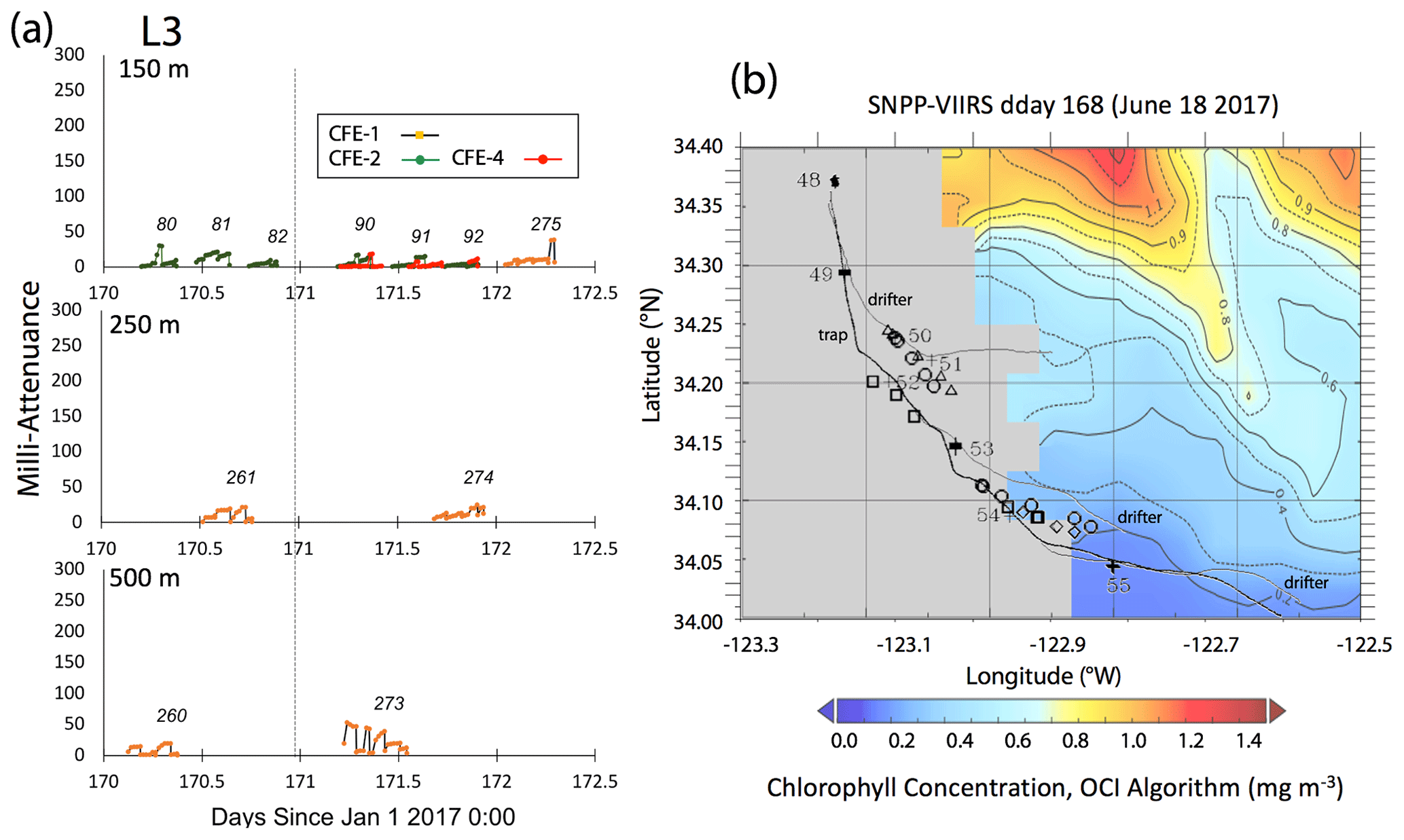
Figure A2(a) Raw attenuance time series for CFEs deployed at L3. See Fig. 2 for deployment context. Italicized numbers are the dive numbers corresponding to the data. (b) Map showing deployment and trajectories of CFEs, CTD station locations, and tracks of the productivity drifter and sediment trap array during the intensive studies at L3. The overlay is the SNPP VIIRS chlorophyll field for 18 June 2017 – prior to deployments. There is no contemporaneous imagery. CTD cast numbers are shown on the plot.
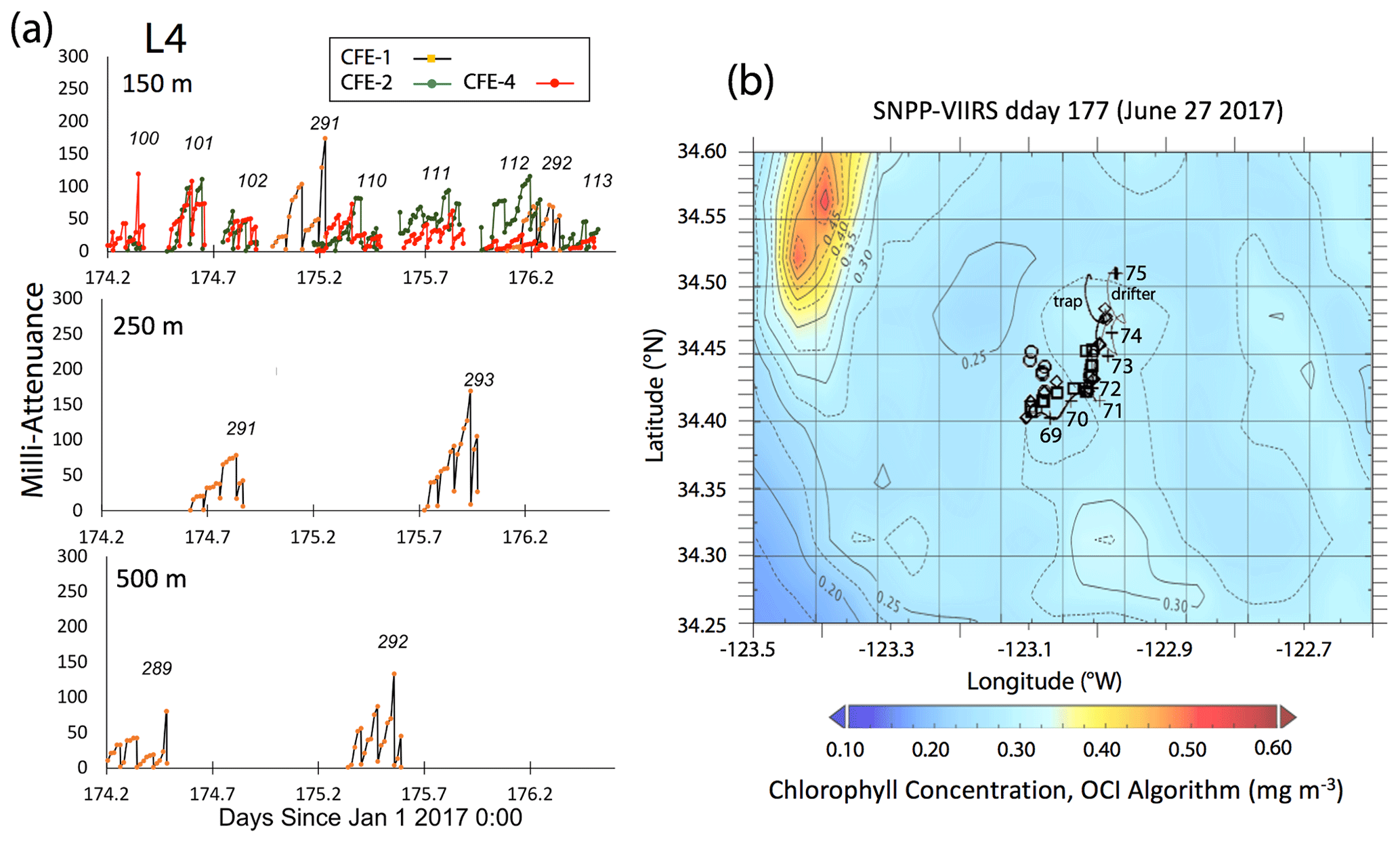
Figure A3(a) Raw attenuance time series for CFEs deployed at L4. See Fig. 2 for deployment context. Italicized numbers are the dive numbers corresponding to the data. (b) Map showing deployment and trajectories of CFEs, CTD station locations, and tracks of the productivity drifter and sediment trap array during the intensive studies at L2. The overlay is the SNPP VIIRS chlorophyll field for 27 June 2017 – at the end of the period. There is no contemporaneous imagery. CTD cast numbers are shown on the plot.
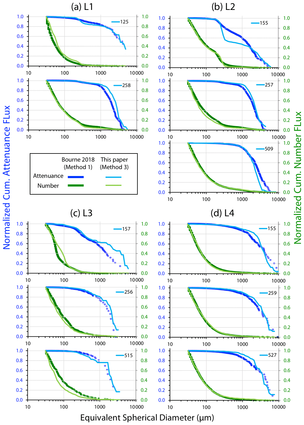
Figure A4Comparison of normalized-cumulative-attenuance flux and normalized-cumulative-number flux size distributions determined using methods 1 (Bourne 2018) and 3 (this paper). The darker thicker lines are results from Method 1. In most cases, the two methods compare well at depths of 250 and 500 m. The 150 m data at L2 reflect touching faecal pellets not resolved by Method 1. The 150 m data at L3 show the effects of Method 1's failure to detect large low-attenuance aggregates.
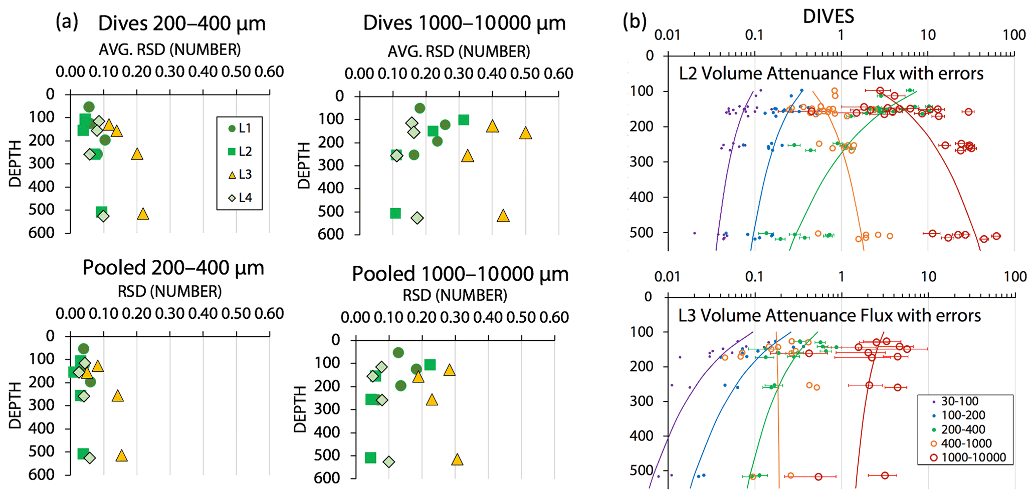
Figure A5(a) Analysis of statistical counting errors for particles in the 200–400 and 1000–10 000 µm size categories. The graphs depict averaged relative standard deviations (RSD) for individual dives and for pooled data at four depth horizons. (b) We illustrate the contribution of statistical counting error and 9 % calibration uncertainty to VAF for the 200–400 and 1000–10 000 µm size categories at L2 and L3. In this case counting errors were based on numbers of particles for each dive. At L2, the contribution of error was a small fraction of the natural variability of >1000 µm VAF results.

Figure A6Scanning electron microscope imagery of an anchovy faecal pellet captured by CFE-Cal at location L1 (see Fig. 14 – L1-125 m). Shown are secondary electron images of the pellet at (a) 244×, (b) 925×, and (c) 2500× magnification. The contents of the pellet are dominated by diatom frustules indicating that anchovies were primary grazers at this location.

Figure A7June 1984 composite of Coastal Zone Colour Scanner retrievals of surface chlorophyll which shows a chlorophyll-rich filament in the vicinity of the VERTEX 1 location. The imagery is sparse by modern standards.
Carbon flux explorer original transmitted light imagery and derived attenuance imagery (∼ 1600 images each) and tabular size analysis results from these images are archived at the Biological and Chemical Oceanography Data Management Office at Woods Hole Oceanographic Institution (https://doi.org/10.26008/1912/bco-dmo.825076.1, Bishop, 2020a; https://doi.org/10.26008/1912/bco-dmo.823408.1, Bishop, 2020b; https://doi.org/10.26008/1912/bco-dmo.825602.1, Bishop, 2020c). The sources of all other data are identified in the text.
The supplement related to this article is available online at: https://doi.org/10.5194/bg-18-3053-2021-supplement.
HLB, as part of her PhD dissertation, played a lead role in precruise laboratory preparation and CFE system assembly and testing. At sea HLB was science lead on deployment and recovery of CFEs. Post cruise HLB led laboratory analysis of samples; she developed fast algorithms capable of running on the CFE in real time and codes that provided physical and hydrographic context for our observations, and she developed the interpretive template for this paper. JKBB served as advisor to HLB during her PhD dissertation and was PI of the project. At sea he maintained CTD-deployed particle concentration sensors and performed all CTD particle optics data reduction. He served as a third hand during CFE deployments and recoveries; post cruise he developed the hybrid particle size analysis codes and analysed remote sensing data sets and worked to bring the paper to publication. TJW was lead on all engineering activities for CFE systems and their precruise ballasting; at sea, he maintained the CFEs and closely worked with HLB on CFE deployments, operations, and recoveries. EJC performed size distribution analysis of aggregates and pellets used to validate the refinement of a pellet classification scheme developed by JKBB.
The authors declare that they have no conflict of interest.
This article is part of the special issue “Biogeochemistry in the BGC-Argo era: from process studies to ecosystem forecasts (BG/OS inter-journal SI)”. It is not associated with a conference.
We would like to thank Mark Ohman (chief scientist), Mike Stukel (USF), members of the science party, and the captain and crew of the R/V Revelle for support during the 2017 CCE-LTER process study. Tim Lowe (LBNL, Engineering – design lead) and Lee-Huang Chen (UC Berkeley, Engineering) contributed substantially to project success. We thank Mark Ohman for inviting us to sea and Mike Stukel for feedback and discussion of this paper. We also thank Alejandro Morales (LBNL) and Mike McLune (SIO – Instrument development group). Many UC Berkeley undergraduates aided in CFE related activities at sea and in the laboratory, in particular we thank Casey Fritz, Xiao Fu, Sylvia Targ, Jessica Kendall-Bar and William Kumler. We thank both reviewers for their contributions. US National Science Foundation grants supported the development of both CFE and CFE-Cal systems, Hannah L. Bourne's thesis research, and seagoing activities and the CCE-LTER project (including ship time).
This research has been supported by the National Science Foundation (grant nos. OCE 1538696 and OCE 1637632).
This paper was edited by Alexandre Mignot and reviewed by Giorgio Dall'Olmo and one anonymous referee.
Abbot, M. R. and Barksdale, B.: Phytoplankton Pigment Patterns and Wind Forcing off Central California, J. Geophys. Res.-Oceans, 96, 14649–14667, https://doi.org/10.1029/91JC01207, 1991.
Alonso-González, I. J., Arístegui, J., Vilas, J. C., and Hernández-Guerra, A.: Lateral POC transport and consumption in surface and deep waters of the Canary Current region: A box model study, Global Biogeochem. Cy., 23, GB2007, https://doi.org/10.1029/2008GB003185, 2009.
Bacon, M. P., Cochran, J. K., Hirschberg, D., Hammar, T. R., and Fleer, A. P.: Export flux of carbon at the equator during the eqpac time-series cruises estimated from 234Th measurements, Deep-Sea Res. Pt. II, 43, 1133–1153, https://doi.org/10.1016/0967-0645(96)00016-1, 1996.
Banse, K.: Reflections About Chance in My Career, and on the Top-Down Regulated World, Annu. Rev. Mar. Sci., 5, 1–19, https://doi.org/10.1146/annurev-marine-121211-172359, 2013.
Bathmann, U. V., Noji, T. T., Voss, M., and Peinert, R.: Copepod fecal pellet: abundance, sedimentation and content at a permanent station in the Norwegian Sea in May/June 1986, Mar. Ecol. Prog. Ser., 38, 45–51, https://doi.org/10.3354/meps038045, 1987.
Beaumont, K. L., Nash, and G. V., Davidson, A. T.: Ultrastructure, morphology and flux of microzoo- plankton faecal pellets in an east Antarctic fjord, Mar. Ecol. Prog. Ser., 245, 133–148, https://doi.org/10.3354/meps245133, 2002.
Berline, O., Stemmann, L., Lombard, F., and Gorsky, G.: Impact of appendicularians on detritus and export fluxes: a model approach at DyFAMed site, J. Plankton Res., 33, 855–872, https://doi.org/10.1093/plankt/fbq163, 2011.
Bishop, J. K. B.: Regional extremes in particulate matter composition and flux: effects on the chemistry of the ocean interior, in: Productivity of the ocean present and past, edited by: Berger, W. H., Smetacek, V. S., and Wefer, G., Dahlem Konferenzen, John Wiley and Sons Ltd., Chichester, UK, 117–137, 1989.
Bishop, J. K. B.: Transmissometer Measurement of POC, Deep-Sea Res. Pt. I, 46, 353–369, https://doi.org/10.1016/S0967-0637(98)00069-7, 1999.
Bishop, J. K. B., Stepien, J. C., and Wiebe, P. H.: Particulate matter distributions, chemistry, and flux in the Panama Basin: Response to environmental forcing, Prog. Oceanogr., 17, 1–59, https://doi.org/10.1016/0079-6611(86)90024-8, 1986.
Bishop, J. K. B.: Original transmitted-light imagery and processed attenuance images of sinking particles observed by autonomous Carbon Flux Explorers deployed 100–500 m in the California Current Regime, during the CCE-LTER process study (P1706) between 2 June and 1 July 2017 [dataset], Version 1, Biological and Chemical Oceanography Data Management Office (BCO-DMO), available at: http://lod.bco-dmo.org/id/dataset/825076 (last access: 17 September 2020) or https://doi.org/10.26008/1912/bco-dmo.825076.1, 2020a.
Bishop, J. K. B.: Size fractionated Particulate Carbon Flux 100–500 m measured by autonomous Carbon Flux Explorers deployed during the CCE-LTER process study (P1706) between 2 June and 1 July 2017 in the California Current Regime [dataset], Version 1, Biological and Chemical Oceanography Data Management Office (BCO-DMO), available at: http://lod.bco-dmo.org/id/dataset/823408 (last access: 16 September 2020) or https://doi.org/10.26008/1912/bco-dmo.823408.1, 2020b.
Bishop, J. K. B.: CTD profile data from Carbon Flux Explorers deployed 100–500 m in the California Current Regime, during the CCE-LTER process study (P1706) between 2 June and 1 July 2017 [dataset], Biological and Chemical Oceanography Data Management Office (BCO-DMO), available at: http://lod.bco-dmo.org/id/dataset/825602 (last access: 30 September 2020) or https://doi.org/10.26008/1912/bco-dmo.825602.1, 2020c.
Bishop, J. K. B. and Wood, T. J.: Particulate matter chemistry and dynamics in the twilightzone at VERTIGO ALOHA and K2 sites, Deep-Sea Res. Pt. I, 55, 1684–1706, https://doi.org/10.1016/j.dsr.2008.07.012, 2008.
Bishop, J. K. B. and Wood, T. J.: Year-round observations of carbon biomass and flux variability in the Southern Ocean, Global Biogeochem. Cy., 23, GB2019, https://doi.org/10.1029/2008GB003206, 2009.
Bishop, J. K. B., Ketten D. R., and Edmond, J. M.: The chemistry, biology and vertical flux of particulate matter from the upper 400 m of the Cape Basin in the S. E. Atlantic Ocean, Deep-Sea Res., 25, 1121–1161, https://doi.org/10.1016/0146-6291(78)90010-3, 1978.
Bishop, J. K. B., Wood, T. J., Davis, R. E., and Sherman, J. T.: Robotic observations of enhanced carbon biomass and export at 55∘ during SOFeX, Science, 304, 417–420, https://doi.org/10.1126/science.1087717, 2004.
Bishop, J. K. B., Fong, M. B., and Wood, T. J.: Robotic observations of high wintertime carbon export in California coastal waters, Biogeosciences, 13, 3109–3129, https://doi.org/10.5194/bg-13-3109-2016, 2016.
Bourne, H. L.: Marine Biogeochemical Cycling of Carbon and Cadmium, Ph.D. dissertation, University of California, Berkeley, California, USA, 121 pp., 2018.
Bourne, H. L., Bishop, J. K. B., Wood, T. J., Loew, T. J., and Liu, Y.: Carbon Flux Explorer optical assessment of C, N and P fluxes, Biogeosciences, 16, 1249–1264, https://doi.org/10.5194/bg-16-1249-2019, 2019.
Boss, E., Guidi, L., Richardson, M. J., Stemman, L., Gardner, W. D., Bishop, J. K. B., Anderson, R. F., and Sherrell, R.: Optical techniques for in-situ characterization of particles pertinent to GEOTRACES, Prog. Oceanogr., 133, 43–54, https://doi.org/10.1016/j.pocean.2014.09.007, 2015.
Boyd, P. W. and Trull, T. W.: Understanding the export of biogenic particles in oceanic waters: Is there consensus?, Prog. Oceanogr., 72, 276–312, https://doi.org/10.1016/j.pocean.2006.10.007, 2007.
Boyd, P. W., Claustre, H., Levy, M., Siegel, D. A., and Weber, T.: Multi-faceted particle pumps drive carbon sequestration in the ocean, Nature, 568, 327–335, https://doi.org/10.1038/s41586-019-1098-2, 2019.
Buesseler, K. O., Lamborg, C. H., Boyd, P. W., Lam, P. J., Trull, T. W., Bidigare, R. R., Bishop, J. K., Casciotti, K. L., Dehairs, F., Elskens, M., Honda, M., Karl, D. M., Siegel, D. A., Silver, M. W., Steinberg, D. K., Valdes, J., Van Mooy, B., and Wilson. S.: Revisiting carbon flux through the ocean's twilight zone, Science, 316, 567–571, https://doi.org/10.1126/science.1137959, 2007.
Burd, A. B., Hansell, D. A., Steinberg, D. K., Anderson, T. R., Arístegui, J., Baltar, F., Eaupré, S. R., Buesseler, K. O., DeHairs, F., Jackson, G. A., Kadko, D. C., Koppelmann, R., Lampitt, R. S., Nagata, T., Reinthaler, T., Robinson, C., Robison, B. H., Tamburini, C., and Tanaka, T.: Assessing the apparent imbalance between geochemical and biochemical indicators of meso- and bathypelagic biological activity: What the @$♯! is wrong with present calculations of carbon budgets?, Deep-Sea Res. Pt. II, 57, 1557–1571, https://doi.org/10.1016/j.dsr2.2010.02.022, 2010.
Chase, Z., Strutton, P. G., and Hales, B.: Iron links river runoff and shelf width to phytoplankton biomass along the U.S. West Coast, Geophys. Res. Lett., 316, 567–571, https://doi.org/10.1029/2006GL028069, 2007.
Chung, S. P., Gardner, W. D., Richardson, M. J., Walsh, I. D., and Landry, M. R.: Beam attenuation and micro-organisms: spatial and temporal variations in small particles along 140∘ W during the 1992 JGOFS EqPac transects, Deep-Sea Res. Pt. II, 43, 1205–1226, https://doi.org/10.1016/0967-0645(96)00030-6, 1996.
Collier, R. and Edmond, J. M.: The trace element geochemistry of marine biogenic particulate matter, Prog. Oceanogr., 13, 113–199, https://doi.org/10.1016/0079-6611(84)90008-9, 1984.
Connors, E. J., Bourne, H. L., and Bishop J. K. B.: Depth and Temporal Variation of Aggregate Export from the Biological Carbon Pump in Upwelling California Coastal Waters, in: AGU/ASLO Ocean Sciences Meeting, Portland, Oregon, USA, 11–16 February 2018, Poster BN14D-1059123, 2018.
Conte, M. H., Ralph, N., and Ross, E. H.: Seasonal and interannual variability in deep ocean particle fluxes at the Oceanic Flux Program (OFP)/Bermuda Atlantic Time Series (BATS) site in the western Sargasso Sea near Bermuda, Deep-Sea Res. Pt. II, 48, 1471–1505, https://doi.org/10.1016/S0967-0645(00)00150-8, 2001.
Deutsch, C., Frenzel, H., McWilliams, J. C., Renault, L., Kessouri, F., Howard, E., Liang, J.-H., Bianchi, D., and Yang, S.: Biogeochemical variability in the California Current System, Prog. Oceanogr., https://doi.org/10.1016/j.pocean.2021.102565, online first, 2021.
Dunne, J. P., Armstrong, R. A., Gnanadesikan, A., and Sarmiento, J. L.: Empirical and mechanistic models for the particle export ratio, Global Biogeochem. Cy., 19, GB4026, https://doi.org/10.1029/2004GB002390, 2005.
Ebersbach, F., Trull, T. W., Davies, D. M., and Bray, S. G.: Controls on mesopelagic particle fluxes in the Sub-Antarctic and Polar Frontal Zones in the Southern Ocean south of Australia in summer-Perspectives from free-drifting sediment traps, Deep-Sea Res. Pt. II, 58, 2260–2276, https://doi.org/10.1016/j.dsr2.2011.05.025, 2011.
Eppley, R. and Peterson, B.: Particulate organic matter flux and planktonic new production in the deep ocean, Nature, 282, 677–680, https://doi.org/10.1038/282677a0, 1979.
Estapa, M. L., Siegel, D. A., Buesseler, K. O., Stanley, R. H. R., Lomas, M. W., and Nelson, N. B.: Decoupling of net community and export production on submesoscales in the Sargasso Sea, Global Biogeochem. Cy., 29, 1266–1282, https://doi.org/10.1002/2014GB004913, 2015.
Gangopadhyay, A., Lermusiaux, P. F. J., Rosenfeld, L., Robinson, A. R., Calado, L., Kim, H. S., Leslie, W. G., and Hawley, P. J.: The California Current System: A multiscale overview and the development of a feature-oriented regional modeling system (FORMS), Dynam. Atmos. Oceans, 52, 131–169, https://doi.org/10.1016/j.dynatmoce.2011.04.003, 2011.
Giering, S. L. C., Sanders, R., Martin, A. P., Henson, S. A., Riley, J. S., Marsay, C. M., and Johns, D. G.: Particle flux in the oceans: Challenging the steady state assumption, Global Biogeochem. Cy., 31, 159–171, https://doi.org/10.1002/2016GB005424, 2017.
González, H. E.: Distribution and abundance of minipellets around the Antarctic peninsula, Implications for protistan feeding behaviour, Mar. Ecol. Prog. Ser., 90, 223–236, https://doi.org/10.3354/meps090223, 1992.
González, H. E., Ortiz, V. C., and Sobarzo, M.: The role of faecal material in the particulate organic carbon flux in the northern Humboldt Current, Chile (23∘ S), before and during the 1997–1998 El Niño, J. Plankton Res., 22, 499–529, https://doi.org/10.1093/plankt/22.3.499, 2000.
Gorsky, G. and Fenaux, R.: The role of appendicularia in marine food webs, in: The Biology of Pelagic Tunicates, Oxford University Press, Oxford, UK, 161–169, 1998.
Gowing, M. M.: Abundance and feeding ecology of Antarctic phaeodarian radiolarians, Mar. Biol., 103, 107–118, https://doi.org/10.1007/BF00391069, 1989.
Gruber, N., Lachkar, Z., Frenzel, H., Marchesiello, P., Münnich, M., McWilliams, J. C., Nagai, T., and Plattner, G.-K.: Eddy-induced reduction of biological production in eastern boundary upwelling systems, Nat. Geosci., 4, 787–792, https://doi.org/10.1038/ngeo1273, 2011.
Hansen, J. L. S., Kiorboe, T., and Alldredge, A. L.: Marine snow derived from abandoned larvacean houses: sinking rates, particle content and mechanisms of aggregate formation, Mar. Ecol.-Prog. Ser., 141, 205–215, https://doi.org/10.3354/meps141205, 1996.
Henson, S. A., Sanders, R., Madsen, E., Morris, P. J., Le Moigne, F., and Quartly, G. D.: A reduced estimate of the strength of the ocean's biological carbon pump, Geophys. Res. Lett., 38, 10–14, https://doi.org/10.1029/2011GL046735, 2011.
Johnson, K., Chavez, F., and Friederich, G.: Continental-shelf sediment as a primary source of iron for coastal phytoplankton, Nature, 398, 697–700, https://doi.org/10.1038/19511, 1999.
Johnson, K. S., Plant, J. N., Dunne, J. P., Talley, L. D., and Sarmiento, J. L.: Annual nitrate drawdown observed by SOCCOM profiling floats and the relationship to annual net community production, J. Geophys. Res.-Oceans, 122, 6668–6683, https://doi.org/10.1002/2017JC012839, 2017.
Kelly, T. B., Goericke, R., Kahru, M., Song, M., and Stukel, M. R.: CCE II: Spatial and interannual variability in export efficiency and the biological pump in an eastern boundary current upwelling system with substantial lateral advection, Deep-Sea Res. Pt. I, 140, 14–25, https://doi.org/10.1016/j.dsr.2018.08.007, 2018.
Komar, P. O., Morse, A. P., Small, L. F., and Fowler, S. W.: An analysis of the sinking rates of copepod and euphausiid fecal pellets, Limnol. Oceanogr., 26, 172–180, https://doi.org/10.4319/lo.1981.26.1.0172, 1981.
Kranz, S. A., Wang, S., Kelly, T. B., Stukel, M. R., Goericke, R., Landry, M. R., and Cassar, N.: Lagrangian studies of marine production: A multimethod assessment of productivity relationships in the California Current Ecosystem upwelling region, J. Geophys. Res.-Oceans, 125, e2019JC015984, https://doi.org/10.1029/2019JC015984, 2020.
Krause, M.: Vertical distributions of fecal pellets during FLEX'76, Helgolander Meeresun., 34, 313–327, https://doi.org/10.1007/BF02074125, 1981.
Kwon, E. Y., Primeau, F., and Sarmiento, J. L.: The impact of remineralization depth on the air-sea carbon balance, Nat. Geosci., 2, 630–635, https://doi.org/10.1038/ngeo612, 2009.
Lam, P. J. and Bishop, J. K. B.: High biomass, low export regimes in the Southern Ocean, Deep-Sea Res. Pt. II, 54, 601–638, https://doi.org/10.1016/j.dsr2.2007.01.013, 2007.
Lam, P. J., Bishop, J. K. B., Henning, C. C., Marcus, M. A., Waychunas, G. A., and Fung, I. Y.: Wintertime phytoplankton bloom in the Subarctic Pacific supported by Continental Shelf Iron, Global Biogeochem. Cy., 20, GB1006, https://doi.org/10.1029/2005GB002557, 2006.
Lerman, A., Lal, D., and Dacey, M. F.: Stokes' settling and chemical reactivity of suspended particles in natural waters, in: Suspended solids in water, edited by: Gibbs, R. J., Plenum Press, New York, https://doi.org/10.1007/978-1-4684-8529-5, 17–47, 1975.
Li, Z. and Cassar, N.: Satellite estimates of net community production based on observations and comparisons to other estimates, Global Biogeochem. Cy., 30, 735–752, https://doi.org/10.1002/2015GB005314, 2016.
Lutz, M., Caldeira, K., Dunbar, R., and Behrenfeld, M.: Seasonal rhythms of net primary production and particulate organic carbon flux to depth describe the efficiency of biological pump in the global ocean, J. Geophys. Res.-Oceans, 112, C10011, https://doi.org/10.1029/2006JC003706, 2007.
Lynn, R. J. and Simpson, J. J.: The California Current System: The Seasonal Variability of its Physical Characteristics, J. Geophys. Res.-Oceans, 92, 12947–12966, https://doi.org/10.1029/JC092iC12p12947, 1987.
Madin, L. P. and Purcell, J. E.: Feeding, metabolism and growth of Cyclosapa Bakeri in the subarctic Pacific, Limnol. Oceanogr., 37, 1236–1251, https://doi.org/10.4319/lo.1992.37.6.1236, 1992.
Marsay, C. M., Sanders, R. J., Henson, S., Pabortsava, K., and Achterberg, E. P.: Attenuation of sinking particulate organic carbon flux through the mesopelagic ocean, P. Natl. Acad. Sci. USA, 112, 1089–1094, https://doi.org/10.1073/pnas.1415311112, 2015.
Martin, J. H., Knauer, G. A., Karl, D. M., and Broenkow, W. W.: VERTEX: carbon cycling in the northeast Pacific, Deep-Sea Res., 34, 267–285, https://doi.org/10.1016/0198-0149(87)90086-0, 1987.
McPhee-Shaw, E. E., Sternberg, R. W., Mullenbach, B., and Ogston, A. S.: Observations of intermediate nepheloid layers on the northern California continental margin, Cont. Shelf Res., 24, 693–720, https://doi.org/10.1016/j.csr.2004.01.004, 2004.
Ohman, M., Barbeau, K., Franks, P., Goericke, R., Landry, M., and Miller, A.: Ecological Transitions in a Coastal Upwelling Ecosystem, Oceanography, 26, 210–219, https://doi.org/10.5670/oceanog.2013.65, 2013.
Omand, M. M., Asaro, E. A., Lee, C. M., Perry, M. J., Briggs, N., Cetinić, I., and Mahadevan, A.: Eddy-driven subduction exports particulate organic carbon from the spring bloom, Science, 348, 222–225, https://doi.org/10.1126/science.1260062, 2015.
Pak, H., Zaneveld, R. V., and Kitchen J.: Intermediate Nepheloid Layers Observed off Oregon and Washington, J. Geophys. Res.-Oceans, 85, 6697–6708, https://doi.org/10.1029/JC085iC11p06697, 1980.
Passow, U. and Carlson, C. A.: The biological pump in a high CO2 world, Mar. Ecol. Prog. Ser., 470, 249–271, https://doi.org/10.3354/meps09985, 2012.
Pomeroy, L. R., Hanson, R. B., McGillivary, P. A., Sherr, B. F., Kirchman, D., and Deibel, D.: Microbiology and chemistry of fecal products of pelagic turnicates: rates and fates, B. Mar. Sci., 35, 426–439, 1984.
Saba, G. K. and Steinberg, D. K.: Abundance, composition, and sinking rates of fish fecal pellets in the santa barbara channel, Sci. Rep.-UK, 2, 716, https://doi.org/10.1038/srep00716, 2012.
Sasaki, H., Hattori, H., and Nishizawa, S.: Downward flux of particulate organic matter and vertical distribution of calanoid copepods in the Oyasio Waters in the summer, Deep-Sea Res., 35, 505–515, https://doi.org/10.1016/0198-0149(88)90128-8, 1988.
Sato, R., Tanaka, Y., and Ishimaru, T.: House Production by Oikopleura dioica (Tunicata, Appendicularia) Under Laboratory Conditions, J. Plankton Res., 23, 415–423, https://doi.org/10.1093/plankt/23.4.415, 2001.
Schneider, N., Lorenzo, E. D., and Niler, P. P.: Salinity Variations in the Southern California Current, J. Phys. Oceanogr., 35, 1421–1436, https://doi.org/10.1175/JPO2759.1, 2005.
Siegel, D. A., Buesseler, K. O., Doney, S. C., Sailley, S. F., Behrenfeld, M. J., and Boyd, P. W.: Global assessment of ocean carbon export by combining satellite observations and food-web models, Global Biogeochem. Cy., 28, 181–196, https://doi.org/10.1002/2013GB004743, 2014.
Siegel, D. A., Buesseler, K. O., Behrenfeld, M. J., Benitez-Nelson, C. R., Boss, E., Brzezinski, M. A., Burd, A., Carlson, C. A., D'Asaro, E. A., Doney, S. C., Perry, M. J., Stanley, R. H. R., and Steinberg, D. K.: Prediction of the Export and Fate of Global Ocean Net Primary Production: The EXPORTS Science Plan, Frontiers in Marine Science, 3, 22, https://doi.org/10.3389/fmars.2016.00022, 2016.
Siegelman-Charbit, L., Koslow, J. A., Jacox, M. G., Hazen, E. L., Bograd, S. J., and Miller, E. F.: Physical forcing on fish abundance in the southern California Current System, Fish. Oceanogr., 27, 475–488, https://doi.org/10.1111/fog.12267, 2018.
Silver, M. W., Coale, S. L., Pilskaln, C. H., and Steinberg, D. R.: Giant aggregates: Importance as microbial centers and agents of material flux in the mesopelagic zone, Limnol. Oceanogr., 43, 498–507, https://doi.org/10.4319/lo.1998.43.3.0498, 1998.
Smetacek, V. S.: Zooplankton standing stock, copepod faecal pellets and particulate detritus in Kiel bight, Estuar. Coast. Mar. Sci., 11, 477–490, https://doi.org/10.1016/S0302-3524(80)80001-6, 1980.
Stanley, R. H. R., Doney, S. C., Jenkins, W. J., and Lott, III, D. E.: Apparent oxygen utilization rates calculated from tritium and helium-3 profiles at the Bermuda Atlantic Time-series Study site, Biogeosciences, 9, 1969–1983, https://doi.org/10.5194/bg-9-1969-2012, 2012.
Steinberg, D. K., Van Mooy, B. A. S., Buesseler, K. O., Boyd, P. W., Kobari, T., and Karl, D. M.: Bacterial vs. zooplankton control of sinking particle flux in the ocean's twilight zone, Limnol. Oceanogr., 53, 1327–1338, https://doi.org/10.4319/lo.2008.53.4.1327, 2008.
Stemmann, L., Prieur, L., Legendre, L., Taupier-Letage, I., Picheral, M., Guidi, L., and Gorsky, G.: Effects of frontal processes on marine aggregate dynamics and fluxes: an interannual study in a permanent geostrophic front (NW Mediterranean), J. Marine Syst., 70, 1–20, https://doi.org/10.1016/j.jmarsys.2007.02.014, 2008.
Stukel, M. and Landry, M.: California Current Ecosystem LTER: Exported particulate carbon and nitrogen measurements from 4-day sediment trap deployments in the CCE region, 2007–2017 (ongoing), version 6, Environmental Data Initiative, available at: https://doi.org/10.6073/pasta/de679918c44266dcebbc5f85a37dcd36, 2020.
Stukel, M. R., Ohman, M. D., Benitez-Nelson, C. R., and Landry, M. R.: Contributions of mesozooplankton to vertical carbon export in a coastal upwelling system, Mar. Ecol. Prog. Ser., 491, 47–65, https://doi.org/10.3354/meps10453, 2013.
Stukel, M. R., Asher, E., Couto, N., Schofield, O., Strebel, S., Tortell, P., and Ducklow, H. W.: The imbalance of new and export production in the western Antarctic Peninsula, a potentially “leaky” ecosystem, Global Biogeochem. Cy., 29, 1400–1420, https://doi.org/10.1002/2015GB005211, 2015.
Stukel, M. R., Song, H., Goericke, R., and Miller, A. J.: The role of subduction and gravitational sinking in particle export, carbon sequestration, and the remineralization length scale in the California Current Ecosystem, Limnol. Oceanogr., 63, 363–383, https://doi.org/10.1002/lno.10636, 2018.
Turner, J. T.: Progress in Oceanography Zooplankton fecal pellets, marine snow, phytodetritus and the ocean's biological pump, Prog. Oceanogr., 130, 205–248, https://doi.org/10.1016/j.pocean.2014.08.005, 2015.
Whitmore, B. M., Nickels, C. F., and Ohman, M. D.: A comparison between Zooglider and shipboard net and acoustic mesozooplankton sensing systems, J. Plankton Res., 41, 521–533 https://doi.org/10.1093/plankt/fbz033, 2019.
Wong, C. S., Whitney, F. A., Crawford, D. W., Iseki, K., Matear, R. J., Johnson, W. K., Page, J. S., and Timothy, D.: Seasonal and interannual variability in particle fluxes of carbon, nitrogen and silicon from time series of sediment traps at Ocean Station P, 1982–1993: relationship to changes in subarctic primary productivity, Deep-Sea Res. Pt. II, 46, 2735–2760, https://doi.org/10.1016/S0967-0645(99)00082-X, 1999.
Yao, X. and Schlitzer, R.: Assimilating water column and satellite data for marine export production estimation, Geosci. Model Dev., 6, 1575–1590, https://doi.org/10.5194/gmd-6-1575-2013, 2013.