the Creative Commons Attribution 4.0 License.
the Creative Commons Attribution 4.0 License.
 | 04 Jun 2021
Recent above-ground biomass changes in central Chukotka (Russian Far East) using field sampling and Landsat satellite data
Ulrike Herzschuh
Birgit Heim
Luise Schulte
Simone Stünzi
Luidmila A. Pestryakova
Evgeniy S. Zakharov
Upscaling plant biomass distribution and dynamics is essential for estimating carbon stocks and carbon balance. In this respect, the Russian Far East is among the least investigated sub-Arctic regions despite its known vegetation sensitivity to ongoing warming. We representatively harvested above-ground biomass (AGB; separated by dominant taxa) at 40 sampling plots in central Chukotka. We used ordination to relate field-based taxa projective cover and Landsat-derived vegetation indices. A general additive model was used to link the ordination scores to AGB. We then mapped AGB for paired Landsat-derived time slices (i.e. 2000/2001/2002 and 2016/2017), in four study regions covering a wide vegetation gradient from closed-canopy larch forests to barren alpine tundra. We provide AGB estimates and changes in AGB that were previously lacking for central Chukotka at a high spatial resolution and a detailed description of taxonomical contributions. Generally, AGB in the study region ranges from 0 to 16 kg m−2, with Cajander larch providing the highest contribution. Comparison of changes in AGB within the investigated period shows that the greatest changes (up to 1.25 kg m−2 yr−1) occurred in the northern taiga and in areas where land cover changed to larch closed-canopy forest. As well as the notable changes, increases in AGB also occur within the land-cover classes. Our estimations indicate a general increase in total AGB throughout the investigated tundra–taiga and northern taiga, whereas the tundra showed no evidence of change in AGB.
- Article
(8098 KB) - Full-text XML
- BibTeX
- EndNote


Estimated global mean surface temperature has increased by 0.87 ∘C since pre-industrial times and continues to rise (IPCC, 2018). The Arctic is warming 2 to 3 times faster than the global annual average. Here, vast amounts of terrestrial carbon are stored in the soil organic matter and living plant biomass (McGuier et al., 2009; ACIA, 2005), and, therefore, changes in the carbon cycle potentially affected by climate change are a central issue. In the course of global warming, positive feedbacks can be observed: for example, encroachment of deep-rooted vegetation due to shrubification can lead to deeper carbon deposition and act as a potential carbon sink (Jobbágy and Jackson, 2000). Therefore, estimation of above-ground biomass (AGB) stocks and detailed knowledge about the individual taxa contributing to it is of prime interest in understanding whether the northernmost forests and tundra also change in biomass in analogy to the widespread observed shrubification. This information is essential for modelling terrestrial carbon cycling in vulnerable high-latitude ecosystems and will help predict future carbon dynamics that may accelerate or slow down future warming.
Detailed (species/taxa level) estimation of AGB can provide more valuable information on an ecosystem's functioning and its development than AGB estimates at a plant functional type (PFT) level. For example, a loss of specific species from one PFT can be replaced by taxa from another PFT in response to climate change even though total AGB production remains similar (Bret-Harte et al., 2008). Thus, the change in AGB between PFTs can be caused by changing species contributions within PFTs. However, many studies of Arctic and sub-Arctic regions present AGB state or change at a PFT level (Räsänen et al., 2018; Berner et al., 2018; Webb et al., 2017; Walker et al., 2003). Some focus only on shrub biomass of one or more species (Vankoughnett and Grogan, 2015; Berner et al., 2018), while others focus on tree biomass (Berner et al., 2012) or on species and PFT AGB of one specific community (e.g. Hudson and Henry, 2009). Occasionally, a study presents results of AGB on a PFT level despite sampling methods that suggest a division by species in the field (Maslov et al., 2016; Chen et al., 2009). Very seldom is AGB presented at a species/taxa level (e.g. Shaver and Chapin, 1991). In consequence, only a few estimations of species or taxon-specific AGB are available to assess species/taxa contributions.
Whereas for some Arctic regions in North America, AGB state and change have been well studied (e.g. Canada in Hudson, 2009), the Russian Far East has received less attention and AGB has never been investigated in the vast areas of central Chukotka, which is our study region. The very few existing circumpolar AGB estimations that also cover these areas (Raynolds et al., 2011; Santoro and Cartus, 2019) have a coarse spatial resolution (1 km and 100 m, respectively) and, therefore, show only the general AGB gradient of the lowest in tundra to the highest in taiga. Similarly, the circumpolar estimation of Epstein et al. (2012) covers AGB change until 2010 and shows only a general zonal pattern of change. In consequence, it remains unknown how the landscape of central Chukotka, with its characteristic treeline formed by needle-leaf deciduous trees, mountainous terrain, and high diversity of vegetation communities, responds to climate warming in terms of terrestrial carbon stocks.
For vegetation and AGB investigations the remote-sensing index – the normalised difference vegetation index (NDVI) – is often used. It incorporates information from red and near-infra-red regions of the light spectrum that reflect plant biomass of various ecological systems (Pettorelli, 2005). In the Arctic and sub-Arctic regions remote-sensing algorithms based on satellite-derived NDVI and field measurements have been used to predict the total and exclusively shrub AGB in Alaska (Epstein et al., 2008; Berner et al., 2018) and for Cajander larch in north-eastern Siberia (Berner et al., 2012). Some studies have used very high spatial resolution imagery (Räsanen et al., 2018) and hyperspectral field spectrometry for AGB investigations in north-western and northern Siberia and Alaska (Bratsch, 2017) that enable spatially restricted studies on estimations of local AGB. However, the NDVI can be affected by water content and tall vegetation shadows, which can influence the spectral signal of vegetated land (Pattison et al., 2015) and decouple it from the biomass relationship. Such decoupling or similar biomass ranges make distinguishing between different plant functional types (PFT) or communities difficult. Furthermore, the NDVI may not capture differences in the understorey of moderately closed forests (Loranty et al., 2018) because the remote-sensing signal comes from the top of the canopy.
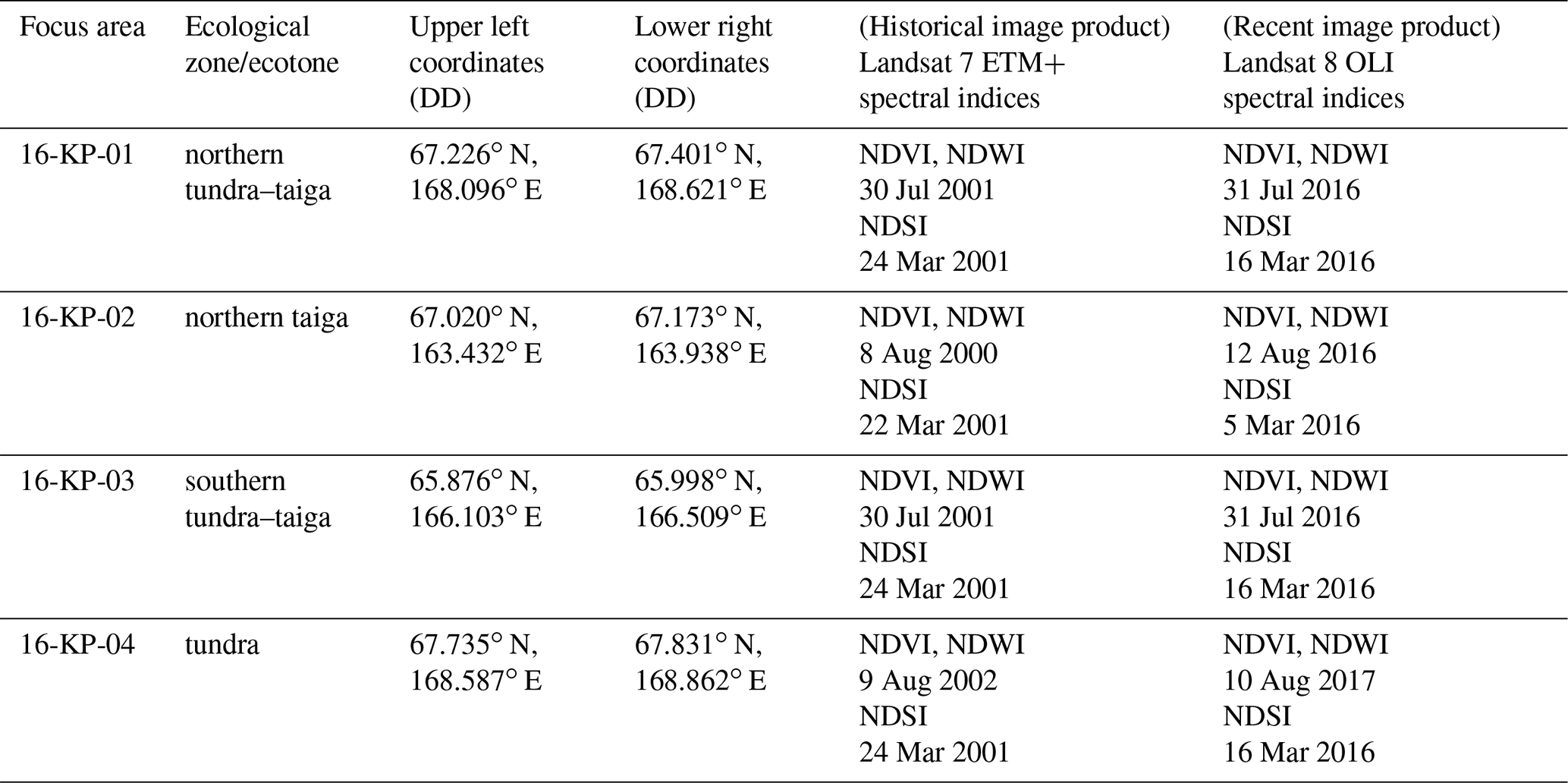
To capture land cover and land-cover change in central Chukotka related to taxa, Shevtsova et al. (2020a) established a redundancy analysis (RDA) model that incorporates the Landsat NDVI, normalised difference water index (NDWI), and normalised difference snow index (NDSI). This model, together with the extensive Landsat satellite data archive, also made it possible to assess the strength and direction of AGB changes in central Chukotka over the last few decades. We used Landsat satellite data and field data from a 2018 expedition in a statistical model for AGB mapping. The aim was to provide an estimation of AGB stocks and their change between paired time points (2000/2001/2002 to 2016/2017) at four focus areas along a tundra–taiga gradient, in central Chukotka. Our first objective was to reconstruct the AGB of each sampling plot using individual plant biomass samples and their corresponding distribution within these plots. The second objective was to upscale AGB in the focus areas for the most recent time covered by Landsat 8 satellite data via statistical modelling. Finally, the third objective was to apply the developed upscaling approach to the oldest available good-quality Landsat 7 acquisitions to investigate AGB changes in the focus areas.
2.1 Study region and field surveys
Our study covers six areas of central Chukotka, Russian Far East (Fig. 1). Four of them (16-KP-01, 16-KP-02, 16-KP-03, 16-KP-04) are our focus areas for biomass mapping and previous vegetation investigations (Shevtsova et al., 2020a); two further areas (18-BIL-01, 18-BIL-02) are supplementary and were investigated for representative AGB sampling. All investigated areas are underlain by continuous permafrost, and all four focus areas are mountainous.
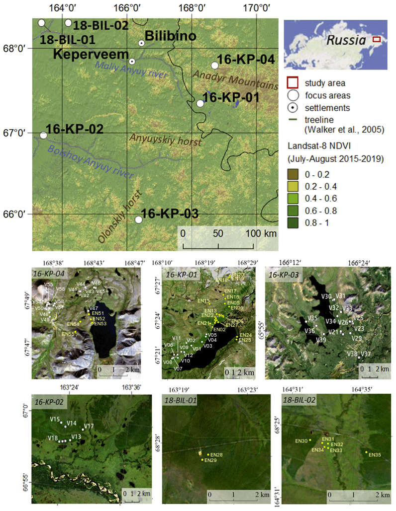
Figure 1Overview of the study region and four focus areas – tundra (16-KP-04), northern tundra–taiga (16-KP-01), southern tundra–taiga (16-KP-03), and northern taiga (16-KP-02) – and two areas with supplementary AGB sampling – 18-BIL-01 and 18-BIL-02 (tundra–taiga to northern taiga). Sample plot names of the 2016 expedition are V01–V58, sample plot names of the 2018 expedition are EN01–EN55 (abbreviated here to EN# rather than EN18#). Overview map modified from Shevtsova et al. (2020a). Base maps of study areas are Landsat 8 RGB composites. Black colour represents no data or water.
During the expedition “Chukotka 2018” in July 2018, we inventoried 40 sample plots (Fig. 1; Biskaborn et al., 2019): 5 sample plots in treeless tundra (16-KP-04), 27 sample plots in the tundra–taiga ecotone (16-KP-01), and 8 sample plots in northern taiga (18-BIL-01, 18-BIL-02). Numbers of plots per habitat are different but align with the concept of stratified random sampling by placing a higher number of plots in the well-represented typical habitats and fewer in the atypical habitats. In the most homogeneous locations, 15 m radius sampling plots were demarcated. Heterogeneity was accommodated by roughly assorting vegetation into two to three vegetation types per sampling plot. Within each area of roughly estimated vegetation types we selected three representative 2 × 2 m subplots for ground-layer foliage projective cover assessment. In these subplots, a 50 × 50 cm area was selected for ground-layer AGB harvesting (major taxa and others), as well as a 10 × 10 cm area for moss and lichen biomass harvesting (Fig. 2). Trees and tall shrubs were sampled directly from the 15 m radius plots. AGB was sampled in 38 sample plots of the 40 inventoried.
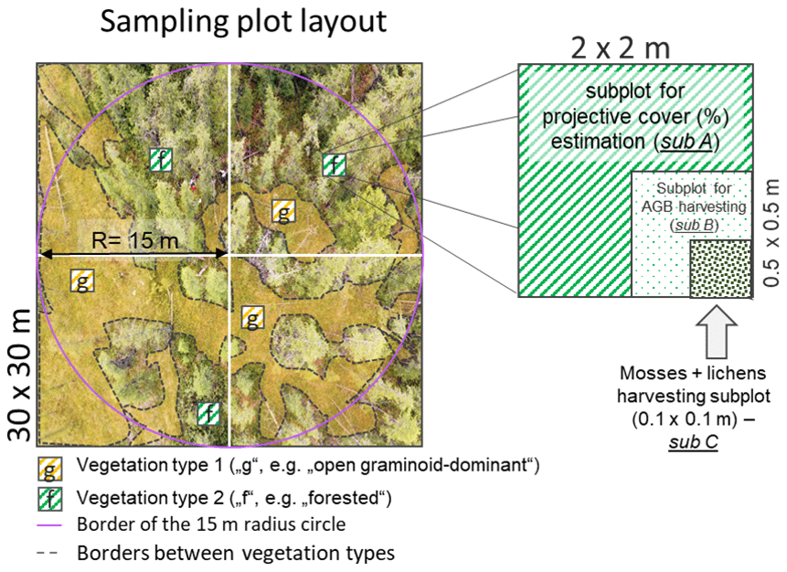
Figure 2Sampling scheme of the 2018 expedition vegetation survey. Projective cover of tall shrubs and trees was estimated on a circular sample plot with a radius of 15 m, while ground-vegetation type cover was estimated on a 30 × 30 m sample plot. To accommodate heterogeneity in the main 30 × 30 m sample plot, two to three dominant vegetation types were identified (e.g. in this example “g” and “f”). Within every vegetation type, three sampling subplots (sub A, 2 × 2 m) were placed for projective cover estimation. Inside one of these, the most representative subplot per vegetation type, we placed a subplot (sub B, 0.5 × 0.5 m) for harvesting above-ground biomass (AGB) from the ground-layer plants, excluding mosses and lichens, which were instead sampled from a representative smaller subplot (sub C, 0.1 × 0.1 m).
All biomass samples were weighed fresh in the field. In general, biomass samples with a weight of more than 15 g were subsampled to reduce the volume of biomass as there were limits to what was logistically possible to transport to the laboratory for drying. All samples were oven dried (60 ∘C, 24 h for ground-layer and moss and lichen samples, 48 h for shrub and tree branch samples, up to 1 week for tree stem discs) and weighed again.
Our 2018 vegetation and biomass sampling plots were consistently placed in similar vegetation communities to those investigated in 2016. In 2016, we investigated only projective cover, whereas in 2018 both projective cover and AGB were estimated. Only tall dense Alnus viridis ssp. fruticosa (Rupr.) Nyman (hereafter Alnus fruticosa) shrub associations were not sampled during the expedition in 2018; this association is a rare type of vegetation community that only occurs in a few places in the area of interest. Additionally, we sampled the vegetation at an old fire scar, mostly consisting of patches of tall non-creeping Salix spp. shrubs with graminoids and dead, upright tree stems of Larix cajanderi Mayr.
The sampling protocols for projective cover and AGB sampling are different for (1) trees (all Larix cajanderi), (2) non-creeping shrubs (Salix spp., Alnus fruticosa, Pinus pumila (Pall.) Regel), and (3) ground-layer plants (including creeping shrubs, herbs, mosses, and lichens).
Tree cover and heights of all trees were visually estimated in the 15 m radius plot after training with a clinometer (Suunto, Finland). Detailed parameters of 10 trees per 15 m radius plot were recorded: height, crown diameter, crown start, stem perimeter at basal and at 1.3 m height, and vitality. We aimed to representatively sample at least three (tall, medium, low) of these trees for AGB. Samples included, if available, needle biomass, one small living branch, one medium-sized living branch, one big living branch, one dead branch, and ideally three stem discs (basal height at 0 cm, breast height at 130 and 260 cm). We estimated the number of branches on each felled tree before felling by eye as follows: (1) number of big branches, (2) number of medium branches on a representative big branch, and (3) number of small branches on a representative medium branch. From the 107 trees sampled, 53 trees were fully sampled, 41 trees were sampled only from the tree trunk, and 13 trees were sampled only from branches and needles. Stem biomass was reconstructed using allometric equations (Appendix A) based on the assumption of a cone-shaped tree form. Using exponential models (Appendix A), we were able to reconstruct total and partial (wood, needle) AGB of all trees (separately for dead and living trees) in each 15 m radius plot. We converted our AGB estimates into averages of kg m−2 for each 15 m radius plot.
Non-creeping shrub cover was estimated in the 15 m radius plot. If present, three representative shrub individuals from each species were sampled for AGB: leaf/needle and branch. The average total and partial AGB from representative shrubs was then converted to kg m−2 for each sample plot (Appendix A).
Ground-layer vegetation cover was estimated in 2 × 2 m representative subplots. AGB of ground-layer plants was estimated by harvesting 50 × 50 cm subplots; AGB of mosses and lichens was estimated by harvesting 10 × 10 cm subplots. By accounting for the vegetation types within each 15 m radius plot, the total average AGB of each sampled taxon was estimated in kg m−2 per sample plot (details in Appendix A).
All AGB estimations (total and per taxon) were analysed in four land-cover classes (1, larch closed-canopy forest; 2, forest tundra and shrub tundra; 3, graminoid tundra; 4, prostrate herb tundra and barren areas; Shevtsova et al., 2020a) and are reported by their median with their interquartile range (IQR) as a measurement of statistical dispersion.
2.2 Above-ground biomass upscaling and change derivation
A redundancy analysis (RDA) model was built with foliage projective cover of 36 taxa from the 2016 expedition sample plots as dependent variables and Landsat spectral indices (normalised difference vegetation index (NDVI), normalised difference water index (NDWI), normalised difference snow index (NDSI)) as predictors (Shevtsova et al., 2020a; Appendix B). We used the RDA model to predict RDA scores for the 40 new sample plots of the 2018 expedition. Foliage projective cover of the new sample plots covered the same taxonomical resolution and was standardised by applying a Hellinger transformation (Legendre and Legendre, 2012). Every position in the ordination space describes a specific vegetation composition with specific coverage, as well as a combination of Landsat spectral indices associated with it. Using the RDA scores, we assigned sample plots from the 2018 expedition to the four established land-cover classes using k-means classification: (1) larch closed-canopy forest, (2) forest tundra and shrub tundra, (3) graminoid tundra, and (4) prostrate herb tundra and barren areas (Shevtsova et al., 2020a).
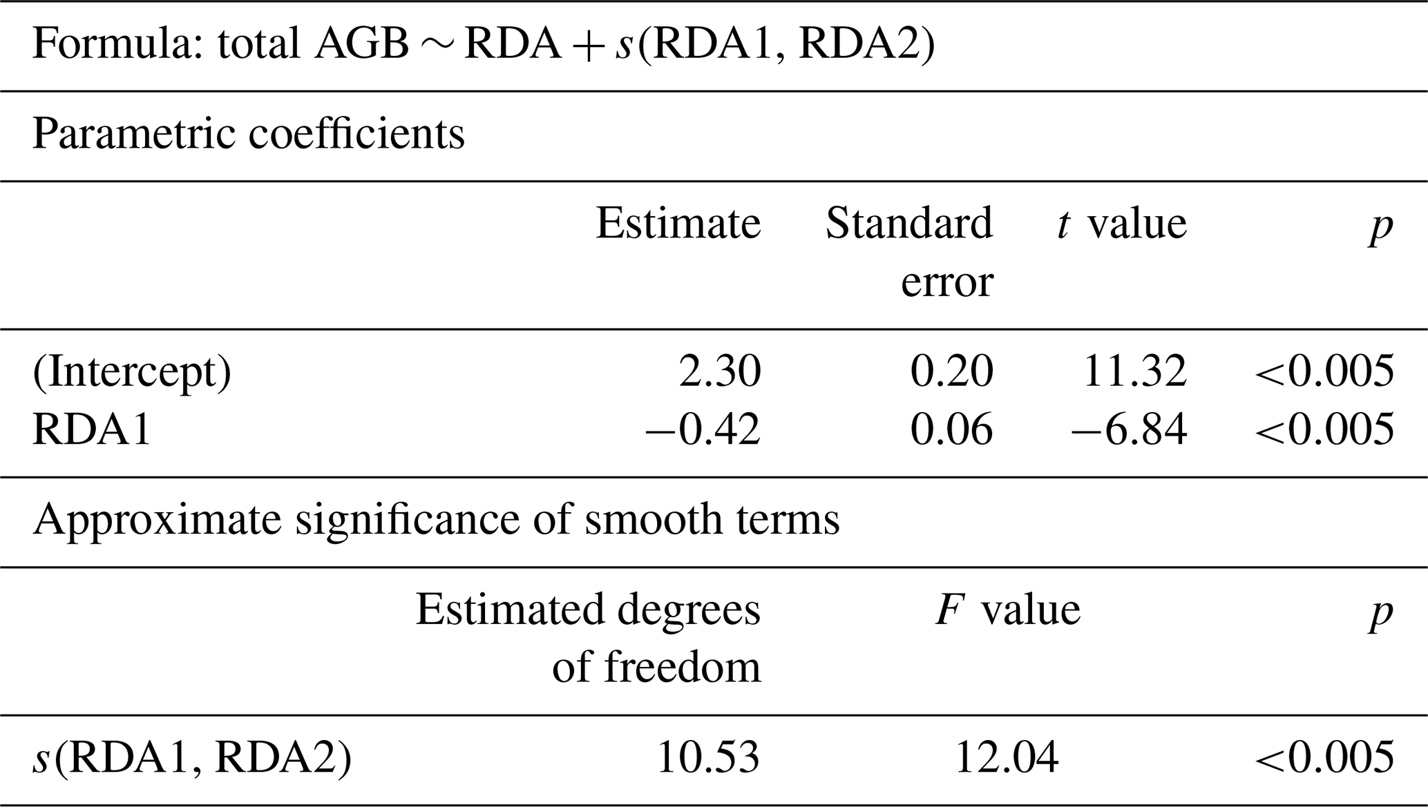
For predicting the total AGB for the 2018 sample plots, the RDA scores of the two first axes were used to build a generalised additive model (GAM; R package “mgcv”) using Eq. (1).
where RDA1 and RDA2 are the ordination scores of the first and second axes, respectively, of the 2018 expedition data from sample plots where AGB was sampled and s is a smooth monotonic function. The parameterised GAM was subsequently used to estimate the total AGB for the four focus areas based on the RDA scores of Landsat spectral indices (Table 1). Specifically, for each focus area the AGB was mapped for each of two time points: recent (2016 or 2017) and historical (2000, 2001, or 2002). From AGB maps with a 15–16 years difference covering the same focus area, AGB change maps were produced. The state of and any change in AGB were estimated within and between land-cover classes for land-cover state and change maps (Shevtsova et al., 2020a). All final estimations of AGB state are presented in kg m−2 as the median with the IQR.
Table 1The four focus areas with corner coordinates (decimal degrees (DD), WGS 84) and acquisition times of the historical and recent Landsat spectral indices (NDVI and NDWI for peak summer, NDSI for snow-covered conditions) used for the redundancy analysis (RDA).
All analyses were performed in R (R Core Team, 2017) using the packages “vegan” version 2.5–4 (Oksanen et al., 2019), “raster” version 2.6–7 (Hijmans, 2017), mgcv (Wood, 2011), “sp” (Pebesma and Bivand, 2005), “factoextra” version 1.0.5.999 (Kassambra and Mundt, 2017), and “ggplot2” (Wickham, 2016).
3.1 Vegetation composition and above-ground biomass
In situ projective cover data of all 2018 expedition vegetation sample plots are described in Shevtsova et al. (2020b). The main vegetation communities of the study region assessed were (1) barren areas, covered only by rock lichens; different vegetation associations of the open tundra such as (2) non-hummock poorly vegetated areas with Dryas octopetala L. and various herbs dominant or (3) hummock tundra with graminoid dominance (Eriophorum vaginatum) and creeping shrubs (Salix spp., Betula nana); (4) high dense Pinus pumila shrub associations; and (5) Larix cajanderi tree stands with different degrees of openness and different understorey compositions.
The predictions of the 40 new sample plots categorised into RDA space assigned 2 sample plots to the class “larch closed-canopy forest”, 17 sample plots to “forest tundra and shrub tundra”, 13 sample plots to “graminoid tundra”, and 7 sample plots to “prostrate herb tundra and barren” (Fig. 3). In situ AGB values for each investigated 2018 expedition vegetation sample plot (Fig. 4) are published in Shevtsova et al. (2020c).
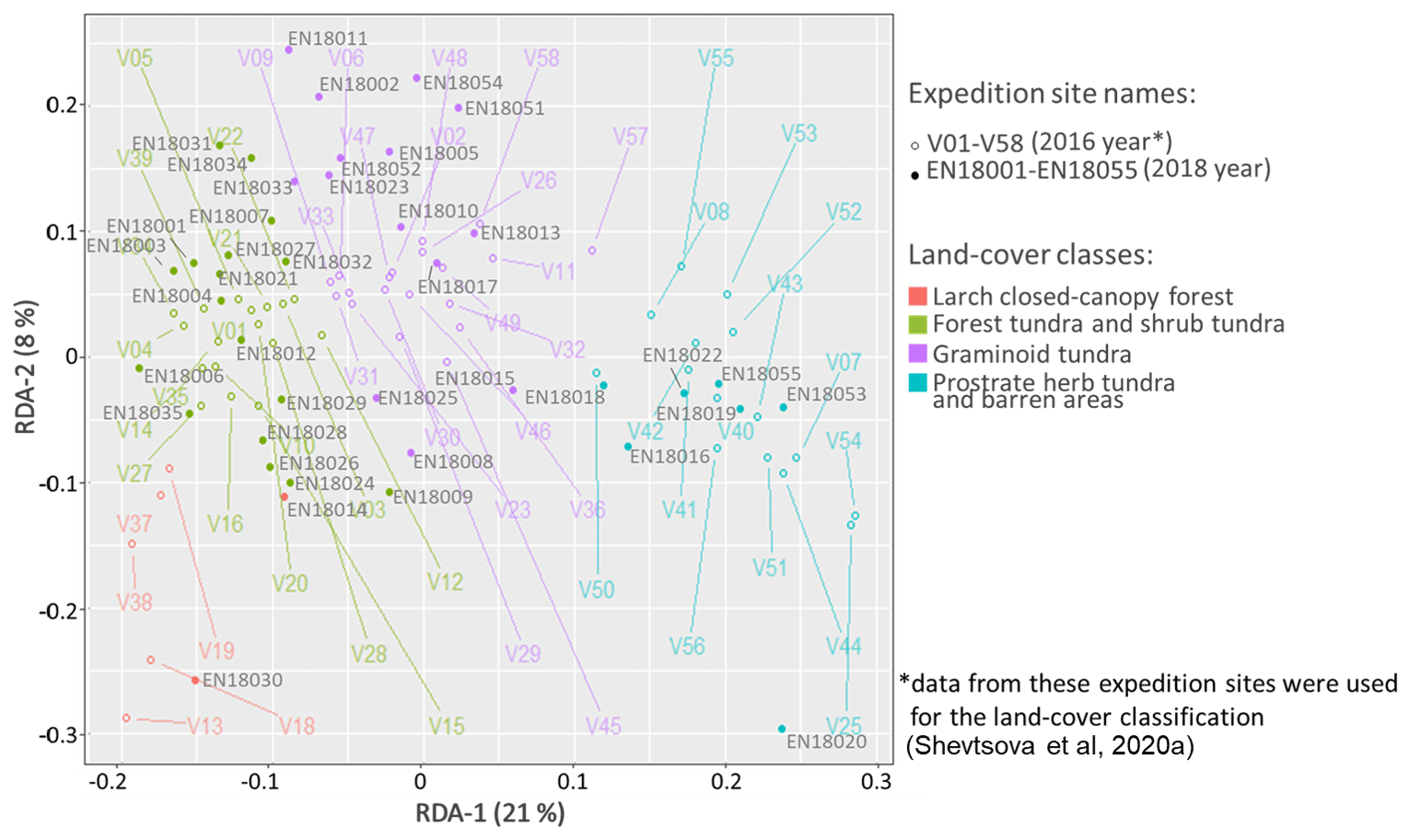
Figure 3Vegetation data of 2018 expedition sorted into RDA space built using the 2016 expedition vegetation data and assigned to four land-cover classes: (1) larch closed-canopy forest, (2) forest tundra and shrub tundra, (3) graminoid tundra, and (4) prostrate herb tundra and barren areas.
In the larch closed-canopy forest L. cajanderi makes the highest contribution to AGB (92 % or 10.20 kg m−2 (IQR = 5.09 kg m−2) on average of the total of 11.04 kg m−2 (IQR = 4.98 kg m−2), Fig. 5). Other major vegetation groups are mosses and lichens (4 %; 0.43 kg m−2 (IQR = 0.004 kg m−2)) and low and dwarf shrubs (4 %; 0.41 kg m−2 (IQR = 0.10 kg m−2)), among them Betula nana ssp. exilis (0.21 kg m−2 (IQR = 0.017 kg m−2)), Ledum palustre L. (0.10 kg m−2 (IQR = 0.019 kg m−2)), Vaccinium vitis-idaea L. (0.08 kg m−2 (IQR = 0.061 kg m−2)), Salix spp. (0.006 kg m−2 (IQR = 0.004 kg m−2)), Empetrum nigrum L. (0.006 kg m−2 (IQR = 0.006 kg m−2)), and V. uliginosum L. (0.003 kg m−2 (IQR = 0.003 kg m−2)).
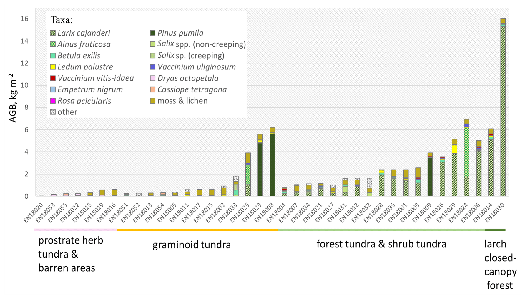
Figure 4In situ above-ground biomass (AGB) in kg m−2 in each investigated sample plot according to the taxa present, ordered by the predicted land-cover class (below names of the sample plots).
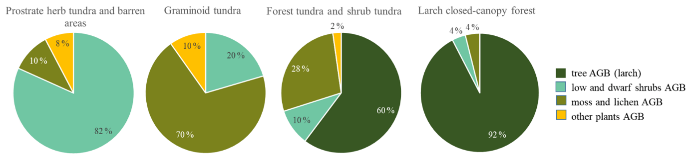
Figure 5Plot-scale average (median) partial AGB in the four vegetation classes. Tall shrubs (Alnus fruticosa, Pinus pumila) were rare and made up less than 1 % of the average plot AGB and are not included here.
In the forest tundra and shrub tundra, 60 % of the average sample plot AGB (1.44 kg m−2 (IQR = 2.40 kg m−2)) is Larix cajanderi which accounts for 0.86 kg m−2 (IQR = 1.45 kg m−2), followed by mosses and lichens (28 %; 0.40 kg m−2 (IQR = 0.19 kg m−2)). Low and dwarf shrubs are 10 % (0.14 kg m−2 (IQR = 0.27 kg m−2) of total sample plot AGB, among them Betula nana (0.05 kg m−2 (IQR = 0.09 kg m−2)), V. vitis-idaea (0.04 kg m−2 (IQR = 0.06 kg m−2)), Ledum palustre (0.03 kg m−2 (IQR = 0.05 kg m−2)), V. uliginosum (0.02 kg m−2 (IQR = 0.06 kg m−2)), Salix spp. (0.003 kg m−2 (IQR = 0.118 kg m−2)), and E. nigrum (0.001 kg m−2 (IQR = 0.010 kg m−2)). The remaining 2 % (0.03 kg m−2 (IQR = 0.01 kg m−2)) are mostly graminoids or other herbs.
In the graminoid tundra, 56 % (0.25 kg m−2 (IQR = 0.32 kg m−2)) of the average sample plot AGB (0.36 kg m−2 (IQR = 1.49 kg m−2)) are mosses and lichens, 20 % (0.07 kg m−2 (IQR = 0.98 kg m−2)) are low and dwarf shrubs, and the remaining 10 % (0.04 kg m−2 (IQR = 0.17 kg m−2)) are other plants (grasses and forbs). Low and dwarf-shrub contributors are B. nana (0.02 kg m−2 (IQR = 0.04 kg m−2)), L. palustre (0.018 kg m−2 (IQR = 0.067 kg m−2)), Salix spp. (0.019 kg m−2 (IQR = 0.03 kg m−2)), V. vitis-idaea (0.013 kg m−2 (IQR = 0.019 kg m−2)), and V. uliginosum (0.008 kg m−2 (IQR = 0.024 kg m−2)).
The average (median) sample plot AGB of the prostrate herb tundra and barren areas is 0.11 kg m−2 (IQR = 0.25 kg m−2), of which 82 % is dwarf-shrub biomass with a dominance of Dryas octopetala (0.07 kg m−2 (IQR = 0.08 kg m−2)) and minor contributions of V. uliginosum (0.006 kg m−2 (IQR = 0.014 kg m−2)), V. vitis-idaea (0.005 kg m−2 (IQR = 0.005 kg m−2)), L. palustre (0.002 kg m−2 (IQR = 0.008 kg m−2)), and Salix spp. (0.001 kg m−2 (IQR = 0.002 kg m−2)). Moss and lichens account for 10 % or 0.11 kg m−2 (IQR = 0.32 kg m−2) of the average sample plot AGB. The other 8 % (0.08 kg m−2 (IQR = 0.08 kg m−2)) of AGB is biomass of different herbs.
Additionally, we analysed the individual partial AGB of four taxa: Larix cajanderi, Alnus fruticosa, Pinus pumila, and non-creeping Salix spp. (Fig. 6). Pinus pumila had a very wide range of needle-to-wood mass ratios, including a ratio indicating a higher weight of needle biomass compared to wood biomass from an individual shrub. For all other investigated species this is not the case. In contrast, deciduous needled larch has the lowest weight ratio of needles to wood when compared to P. pumila, Salix spp., and A. fruticosa. In the different areas of investigation, we observe generally higher leaf (needle)-to-wood mass ratios in the tundra–taiga area (16-KP-01) than in the northern taiga (18-BIL-01, 18-BIL-02).
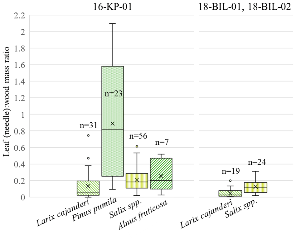
Figure 6Distribution of leaf (needle)-to-wood dry mass ratio among studied species – Larix cajanderi, Pinus pumila, Salix spp. (non-creeping), and Alnus fruticosa – in two ecological regions – tundra–taiga ecotone (16-KP-01) and northern taiga (18-BIL-01, 18-BIL-02); n is number of individuals sampled.
3.2 Upscaling above-ground biomass using GAM
In the GAM, the RDA scores are explanatory variables and total AGB is the dependent variable. The first two RDA axes explain 87 % of the variance in the AGB data (Table 2). Both variables (parametric coefficient RDA1 and the smooth term s(RDA1, RDA2)) are highly significant in the model.
Table 2Estimates and significance values of generalised additive model (GAM) parameters.
We plotted fitted values against residuals for the GAM to visualise residual standard deviations (SDs) for every sample plot used in the modelling (Fig. 7). There is some slight heteroscedasticity, and the SD increases with an increase in absolute AGB values. The RMSE of the model is 1.08 kg.

Figure 7The distribution of residuals of the generalised additive model (GAM) trained for AGB biomass prediction.
Based on the most recent Landsat data acquisitions, the maximum total AGB estimated within our study area is found in the northern taiga in the larch closed-canopy forests (20–24 kg m−2, 16-KP-02, Fig. 8). In the southern tundra–taiga transition (16-KP-03) the maximum AGB reached 12 kg m−2 at places in a river valley that are covered by azonal dense forests. In the northern tundra–taiga (16-KP-01) the maximum AGB is 4–6 kg m−2 in the forest tundra and shrub tundra. In the tundra (16-KP-04) it is 3–4 kg m−2 on the slopes of rivers' valleys.
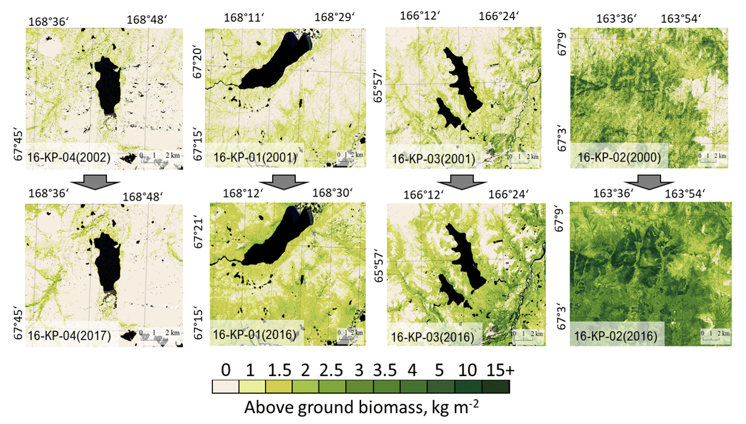
Figure 8Landsat-derived maps of total above-ground biomass (AGB) in historical years (2000, 2001, or 2002) and recent years (2016 or 2017) in four focus areas: treeless tundra (16-KP-04), northern tundra–taiga (16-KP-01), southern tundra–taiga (16-KP-03), and northern taiga (16-KP-770 02).
3.3 Change in above-ground biomass between 2000 and 2017 in the four focus areas
The compiled change maps of recent years (20016/2017) versus 15–16 years earlier (2000/2001/2002) show the rates and spatial patterns of AGB change in the four focus areas (Fig. 9).
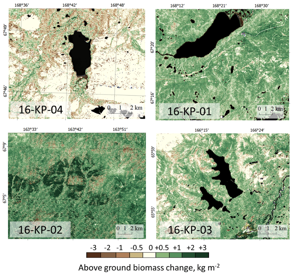
Figure 9Maps of change in Landsat-derived total above-ground biomass (AGB) from historical years (2000/2001/2002) to recent years (20016/2017) in the four focus areas: treeless tundra (16-KP-04), northern tundra–taiga (16-KP-01), southern tundra–taiga (16-KP-03), and northern taiga (16-KP-02). A generally positive trend in AGB change is detected in the tundra–taiga and northern taiga, whereas AGB in the tundra largely remains stable or is decreasing.
Tundra area 16-KP-04, 2002–2017. AGB of prostrate herb tundra vegetation has not changed within the investigated period (0 kg m−2, IQR = 0.12 kg m−2 in 2002 and IQR = 0 kg m−2 in 2017); AGB of graminoid tundra vegetation has slightly decreased (0.69 kg m−2, IQR = 0.83 kg m−2 in 2002; 0.58 kg m−2, IQR = 0.99 kg m−2 in 2017). A change in land-cover class from graminoid tundra to forest tundra and shrub tundra between 2002 and 2017 resulted in AGB increase from 1.42 kg m−2 (IQR = 0.49 kg m−2) to 1.71 kg m−2 (IQR = 0.44 kg m−2), whereas a change from prostrate herb tundra to graminoid tundra resulted in AGB decrease from 0.48 kg m−2 (IQR = 0.87 kg m−2) to 0 kg m−2 (IQR = 0.23 kg m−2).
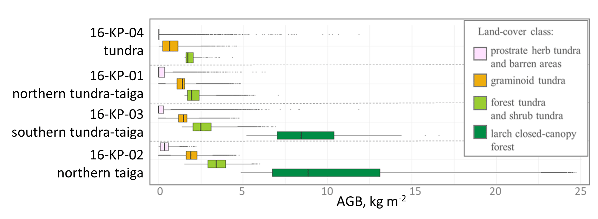
Figure 10Average above-ground biomass (AGB) in recent years (2016/2017) within land-cover classes that have not changed between 2000 and 2017 for four investigated locations, covering a vegetation gradient from tundra (16-KP-04) via tundra–taiga (16-KP-01, 16-KP-03) to northern taiga (16-KP-02).
Northern tundra–taiga area 16-KP-01, 2001–2016. AGB of prostrate herb tundra vegetation stayed stable at 0 kg m−2 (IQR = 0.29 kg m−2 in 2001; IQR = 0.34 kg m−2 in 2016) on average, while the graminoid tundra AGB increased from 0.65 kg m−2 (IQR = 1.04 kg m−2) to 1.40 kg m−2 (IQR = 0.48 kg m−2) and the forest tundra and shrub tundra AGB did not change (1.73 kg m−2, IQR = 0.50 kg m−2 in 2001; 1.70 kg m−2, IQR = 0.32 kg m−2 in 2016). A change in land-cover class from prostrate herb tundra into graminoid tundra resulted in AGB increase from 0 kg m−2 (IQR = 0.24 kg m−2) in 2001 to 0.34 kg m−2 (IQR = 0.67 kg m−2) in 2016, as did a change from graminoid tundra to forest tundra and shrub tundra from 1.27 kg m−2 (IQR = 0.53 kg m−2) in 2001 to 1.69 kg m−2 (IQR = 0.29 kg m2) in 2016.
Southern tundra–taiga area 16-KP-03, 2001–2016. AGB of prostrate herb tundra vegetation did not change and stayed at 0 kg m−2 (IQR = 0.50 kg m−2 in 2001; IQR = 0.31 kg m−2 in 2016) on average, while graminoid tundra AGB increased from 1.00 kg m−2 (IQR = 0.91 kg m−2) in 2001 to 1.50 kg m−2 (IQR = 0.57 kg m−2) in 2016. The forest tundra and shrub tundra AGB only slightly changed (2.00 kg m−2, IQR = 0.99 kg m−2 in 2001; 2.10 kg m−2, IQR = 0.79 kg m−2 in 2016). A change in land-cover class from prostrate herb tundra to graminoid tundra resulted in AGB increase from 0.46 kg m−2 (IQR = 0.82 kg m−2) in 2001 to 0.88 kg m−2 (IQR = 1.03 kg m−2) in 2016, and a change from graminoid tundra to forest tundra and shrub tundra resulted in AGB increase from 1.43 kg m−2 (IQR = 0.48 kg m−2) in 2001 to 2.02 kg m−2 (IQR = 0.66 kg m−2) in 2016. A major AGB change is associated with forest tundra and shrub tundra becoming larch closed-canopy forest resulting in AGB increase from 3.02 kg m−2 (IQR = 1.29 kg m−2) in 2001 to 7.29 kg m−2 (IQR = 2.53 kg m−2) in 2016.
Northern taiga area 16-KP-02, 2000–2016. AGB of prostrate herb tundra vegetation increased from 0 kg m−2 (IQR = 0.09 kg m−2) to 0.60 kg m−2 (IQR = 2.60 kg m−2); graminoid tundra AGB increased from 1.30 kg m−2 (IQR = 0.82 kg m−2) to 1.90 kg m−2 (IQR = 0.69 kg m−2); forest tundra and shrub tundra AGB slightly increased from 2.70 kg m−2 (IQR = 1.33 kg m−2) to 3.10 kg m−2 (IQR = 1.09 kg m−2); and larch closed-canopy forest AGB increased from 7.00 kg m−2 (IQR = 2.49 kg m−2) to 7.50 kg m−2 (IQR = 4.65 kg m−2) within the time studied. A change in land-cover class from prostrate herb tundra into largely graminoid tundra resulted in AGB increase from 0 kg m−2 (IQR = 0.08 kg m−2) in 2000 to 1.45 kg m−2 (IQR = 0.93 kg m−2) in 2016, and a change from graminoid tundra to forest tundra and shrub tundra resulted in AGB increase from 1.44 kg m−2 (IQR = 0.61 kg m−2) in 2000 to 2.78 kg m−2 (IQR = 0.96 kg m−2) in 2016. Some areas classed as forest tundra and shrub tundra became larch closed-canopy forest, which resulted in AGB increase from 3.25 kg m−2 (IQR = 1.49 kg m−2) in 2000 to 7.20 kg m−2 (IQR = 4.12 kg m−2) in 2016.
AGB of land-cover classes that did not change within the investigated period tends to have higher values moving from the tundra to northern taiga (Fig. 10).
We find an increase in AGB for those areas where land-cover class has changed (Table 3). The highest changes in the paired years occurred in the southern tundra–taiga (16-KP-03; +4.30 kg m−2) and the northern taiga (16-KP-02: +4.09 kg m−2) associated with a change in land-cover class from forest tundra and shrub tundra to larch closed-canopy forest. The lowest AGB change rates are associated with a change in land-cover class from graminoid tundra to forest tundra and shrub tundra in the northern taiga (16-KP-02) and southern tundra–taiga (16-KP-03). In general, total AGB in the tundra focus area has not changed over the time studied (0 kg m−2, IQR = 0.2 kg m−2), while in the northern tundra–taiga it has increased by 0.69 kg m−2 (IQR = 0.69 kg m−2) and in the southern tundra–taiga by 0.44 kg m−2 (IQR = 0.91 kg m−2). In the northern taiga total AGB has increased by 1.3 kg m−2 (IQR = 1.4 kg m−2), which is much more than in the other focus areas.
Table 3Above-ground biomass (AGB) change associated with land-cover class change in four focus areas from 2000/2001/2002 to 2016/2017.

4.1 Recent state of above-ground biomass at the field sites
We estimated total and partial dry AGB for the 2018 expedition sample plots, which cover a wide range of vegetation associations (Shevtsova et al., 2020c, d). From these field biomass samples, AGB estimates range from 0 to 15 kg m−2 and, as expected, reflect a gradient of land-cover classes from the least vegetated prostrate herb tundra and barren areas to the larch closed-canopy forests.
As in other subarctic and arctic vegetation studies the taxa found in our study region can be grouped into similar PFTs for a convenient comparison. Thus, deciduous shrubs are largely represented by Betula nana, Vaccinium uliginosum, and Salix sp., which are typical circumpolar subarctic species (Grigoryev, 1946) and are widely found, for example in the tundra in Alaska near Toolik Lake (Shaver and Chapin, 1991). In graminoid tundra, which, by its characteristics, is comparable to tussock tundra in Alaska, deciduous shrubs contribute 33 % to the total AGB (tundra, median = 0.09 kg m−2 and IQR = 0.05 kg m−2) or 9 % (tundra–taiga, median = 0.07 kg m−2 and IQR = 0.05 kg m−2), which is similar to deciduous shrub AGB of Alaskan tussock tundra (0.09 ± 0.02 kg m−2). However, in Alaska, deciduous shrub contribution to the total AGB is 16 %, which is lower than for the central Chukotka graminoid tundra but higher than for the graminoid tundra in the central Chukotkan tundra–taiga. Evergreen shrub taxa are also similar in our study region to those near Toolik Lake, Alaska, being mainly represented by Ledum palustre, Vaccinium vitis-idaea, Dryas octopetala, and Empetrum nigrum, with Pinus pumila in our study region in contrast to Alaska. Evergreen shrubs generally have a lower AGB in the graminoid tundra of our study region (tundra, median = 0.08 and IQR = 0.11; tundra–taiga, median = 0.03 and IQR = 0.10) than in the tussock tundra of Alaska (0.17 ± 0.02 kg m−2), but the percentage of this PFT is slightly higher (31 %) in central Chukotka than in Alaska (24 %). In the graminoid tundra of the central Chukotka tundra–taiga, AGB of evergreen shrubs is poorly represented (4 %). Graminoids in our region were not separately sampled but are included as “other”. However, especially in graminoid tundra, the other class mostly consists of graminoids and other taxa inclusions are rare, so it can be a good approximation of graminoid AGB. The main taxa here, as in Alaska, are Carex sp. and Eriophorum vaginatum. Compared to the tussock tundra in the Toolik Lake vicinity in Alaska, graminoid tundra of both tundra and tundra–taiga areas in central Chukotka has much less graminoid AGB. For the tundra area it is 9 % of total AGB (median = 0.02 kg m−2; IQR = 0.11 kg m−2) and in the tundra–taiga it is 5 % (median = 0.04 kg m−2; IQR = 0.14 kg m−2), whereas in Alaskan tussocks it is 16 % of the total AGB (0.11 ± 0.02 kg m−2). All vascular plant AGB is similar for all compared areas of graminoid/tussock tundra. Graminoid tundra AGB contribution in the tundra area in central Chukotka is 0.25 kg m−2 (median, IQR = 0.04 kg m−2), and in the tundra–taiga area it is 0.34 kg m−2 (median, IQR = 2.46 kg m−2; the high IQR is caused by P. pumila contributions at two sites). This compares to AGB of 0.37 ± 0.03 kg m−2 in the tussock tundra of Alaska. The contribution of vascular plants versus non-vascular plants is much higher in the graminoid tundra of the Chukotka tundra area (96 %) than in Alaska (53 %), whereas for the graminoid tundra of the Chukotka tundra–taiga ecotone their contribution is similar to that in Alaska (42 %). Total AGB of graminoid tundra in central Chukotka is strongly different between tundra (median = 0.26 kg m−2) and tundra–taiga (median = 0.81 kg m−2), with the latter being similar to total AGB of the Alaskan tussock tundra (0.71 kg m−2), while the former is similar to total AGB of open areas and open north-boreal fen in northern Finland (0.30 kg m−2; Räsanen et al., 2018). However, major taxa such as Betula nana, Salix sp., and graminoids have different contributions in these investigated areas. The tundra area in central Chukotka (only graminoid tundra class) has higher AGB from B. nana (median = 0.07 kg m−2; IQR = 0.03 kg m−2) and Salix sp. (median = 0.01 kg m−2; IQR = 0.009 kg m−2) than these taxa in northern Finland (0.02 ± 0.05 and 0.0005 ± 0.008 kg m−2, respectively) but similar AGB of graminoids (0.02 kg m−2, IQR = 0.11 kg m−2 versus 0.03 ± 0.011 kg m−2).
The highest contribution to partial AGB in central Chukotka is from Cajander larch (Larix cajanderi), the only tree species present in the study region. Despite many studies using complex allometric equations, mostly including tree height and stem diameter (e.g. Dong et al., 2020; Alexander et al., 2012; Bjarnadottir et al., 2007) to estimate AGB of an individual tree, we used only tree height because stem diameter measurements (stem perimeter) were not available for all trees. However, where measurements of tree stem diameters were available, these are shown to be highly correlated with height (Appendix A, Fig. A3), which makes it rational to use only height to estimate tree AGB to avoid multicollinearity in the model. Other parameters (crown height, crown width) were also measured on a subset of trees and proved to be insignificant predictors. Thus, using estimated tree height we provide coherent AGB estimation models by accounting for living state (live or dead) and ecological zone (tundra–taiga, northern taiga). We also estimated leaf and wood biomass separately and summed them in the data processing procedure (Appendix A). These established allometric equations can be applied at a broad scale in central Chukotka to a range of tree heights (up to 20 m), as covered by our study.
4.2 Recent state of above-ground biomass upscaled for central Chukotka
The AGB of the studied focus areas of central Chukotka varies along a gradient from <0.5 kg m−2 in the sparsely vegetated areas of the tundra to 25 kg m−2 in the dense larch forests of the northern taiga. When comparing areas in the circumpolar region with a similar vegetation to that of our study region it can be seen that graminoid tundra in central Chukotka generally has less AGB than tussock tundra in Alaska (Toolik research station; Shaver and Chapin, 1991), whereas forest tundra in central Chukotka has more larch AGB than in the Kolyma region (Berner et al., 2018).
Circumpolar remote-sensing-based estimations such as in Santoro and Cartus (2019) and Raynolds et al. (2011) have lower spatial resolution and less precise AGB estimates for central Chukotka than our mapped AGB estimates. The most recent (2017) European Space Agency (ESA) global AGB map (Santoro and Cartus, 2019) shows generally lower AGB estimates for non-mountainous regions of central Chukotka than our AGB estimates: shrublands in tundra with AGB of 1.5–4 kg m−2 (our estimations) only range from 0.3 to 0.6 kg m−2 in the ESA AGB product; our AGB estimates for forest tundra in the tundra–taiga ecotone range from 2.5 to 3 kg m−2 but are 0.07–0.16 kg m−2 in the ESA AGB product; for graminoid tundra in the tundra–taiga ecotone our AGB estimates are 0.7–3 kg m−2, while ESA AGB is 0.1–0.8 kg m−2; and our larch closed-canopy forests AGB estimates are 22–24 kg m−2 versus 2.8–4 kg m−2 in the ESA product. In contrast, mountainous regions show unrealistically high AGB values in the ESA AGB product that are most likely due to topographical artefacts in the synthetic aperture radar (SAR) processing of the ESA AGB product (see also Santoro and Cartus, 2019). However, other spatial distribution patterns of AGB, especially in the tundra–taiga areas (16-KP-01, 16-KP-03) are very similar to our AGB results. The dissimilarities in the AGB magnitudes can be explained by the different remote-sensing methods: the ESA AGB product was derived from SAR remote sensing while our AGB estimates are based on optical Landsat data. SAR-based biomass estimation is sensitive to vegetation structure and can only derive higher vegetation layers. Therefore, ESA AGB can only represent a “living-tree AGB”, while our AGB estimates include other plant groups (lower shrubs, ground vegetation, mosses and lichens) of central Chukotka and are thus more suitable for the investigated area.
Two of our focus areas overlap with the circumpolar above-ground phytomass map of peak-summer season (Raynolds et al., 2011), and a comparison reveals that AGB estimates for the tundra–taiga area (16-KP-01) are similar to each other: 0.65 kg m−2 (IQR = 1.1 kg m−2) in 2001 and 1.5 kg m−2 (IQR = 0.46 kg m−2) in 2016 (our estimates) versus 0.61–0.97 kg m−2 in 2010. However, for the second area, 16-KP-04, our average AGB estimate is lower during the whole investigation period at 0 kg m−2 (IQR = 0.7 kg m−2) in 2002 and 0 kg m−2 (IQR = 0.37 kg m−2) in 2017 versus 0.61–0.97 kg m−2 in 2010 as estimated by Raynolds et al. (2011).
Further comparison with AGB of similar vegetation types in Alaska (Toolik research station; Shaver and Chapin, 1991) shows that tussock tundra has higher AGB in Alaska (0.71 kg m−2) than graminoid tundra in central Chukotka (0.36 kg m−2), despite having a similar composition that includes tussocks and also being dominated by Eriophorum vaginatum. This may be because the AGB of graminoids and forbs in Alaska (0.12 kg m−2) is higher than in central Chukotka (0.04 kg m−2) as is the AGB of dwarf shrubs (0.26 kg m2 versus 0.07 kg m−2). The prostrate herb tundra and barren areas land-cover class in central Chukotka has a similar composition to heath communities in Alaska with evergreen dwarf shrubs and extensive exposed ground. Prostrate herb tundra AGB of central Chukotka is lower (0.11 kg m−2) compared to that of Alaska (0.32 kg m−2), having more lichen and dwarf-shrub biomass. Forest tundra and shrub tundra in central Chukotka is challenging to compare to Alaskan communities, but generally, average AGB in this land-cover class is slightly lower (1.33 kg m−2) than AGB of even shrub-only communities in Alaska (1.39 kg m−2), which are formed of tall deciduous shrubs such as Salix spp. growing on river bars and well-drained floodplains. In contrast to Alaska, forest tundra and shrub tundra in central Chukotka includes mostly dwarf or sparse low shrubs, as well as some tall shrubs and open larch tree stands, and is found on more diverse landscape features than river bars. In addition, the AGB of the central Chukotka tundra and also, partly, the northern tundra–taiga is generally comparable to the AGB of the North Slope of Alaska, which ranges from 0 to 4 kg m−2 (Berner et al., 2018).
Comparing our AGB estimates of Larix cajanderi to those in the area around the river Kolyma (western Chukotka; Berner et al., 2012) – a close match to our study region by vegetation composition and partly by environmental settings – reveals similarities in the spatial patterns of AGB distribution. The highest AGB tends to occur on protected mountain valley slopes in both investigated regions. AGB of Larix cajanderi open forests in the river Kolyma area ranges, on average, from 0.5 to 5 kg m−2, reaching the maximum of 6.7 kg m−2, which is comparable with our forest tundra and shrub tundra AGB assuming a 57 % representation of Larix cajanderi in this land-cover class.
Many factors can influence the AGB estimates such as the number of reference samples, prediction method, and remote-sensing sensor type (optical, radar), as well as spatial and temporal resolution of the satellite imagery and products (Fassnacht et al., 2014). Overall, a comparison with global and circumpolar AGB estimates highlights great improvements in the accuracy of the estimates and a better way to resolve a more landscape related spatial pattern of our AGB estimates for the study region.
4.3 Change in above-ground biomass within the investigated 15–16 years in central Chukotka
We derived total AGB changes in the central Chukotka from Landsat satellite data spanning 15–16 years and found the greatest change in the dense forests of the northern taiga (16-KP-02). In the northern tundra–taiga area (16-KP-01), AGB increased from 2001 to 2016 by 0.046 kg m−2 yr−1 (IQR = 0.046 kg m−2 yr−1), which is much faster than the rate estimated by Epstein et al. (2012) for 1982 to 2010 (0.004–0.015 kg m−2 yr−1). Further, we estimated AGB change from 2002 to 2017 in the tundra focus area (16-KP-04) as being close to 0 kg m−2 yr−1 (IQR = 0.013 kg m−2 yr−1) on average, which is lower than estimations from 1982 to 2010 given in the circumpolar above-ground phytomass map for the Russian Far East (Walker and Raynolds, 2018). Our results of tundra AGB change being close to zero are similar to experiments with modelling extreme temperature increases in Alaskan tundra (Hobbie and Chapin, 1998). In their study, Hobbie and Chapin (1998) conclude that, in tundra, plant biomass accumulation depends on nutrient availability and AGB will only increase if mineralisation of soil organic nutrients is stimulated together with climate warming. Given differences in soil development between the focus areas of tundra, tundra–taiga, and northern taiga, their conclusion may also apply to our results. In general, the comparison with circumpolar estimated AGB changes from 1982 to 2010 (Walker and Raynolds, 2018) shows that changes in AGB in our focus areas of central Chukotka between 2000 and 2017 were much faster, probably because of the stronger warming in the first decades of the 21st century in these regions.
Our estimates of AGB change within our land-cover classes show that AGB change does not necessarily lead to a change in land-cover class. We assume that changes for different regions within the same stable land-cover classes could be associated with population size change but also likely with changes in the plant's parameters (height, crown density, etc.). This could explain why the change in AGB estimated for the graminoid tundra in the northern taiga (16-KP-02) is greater than for the tundra (16-KP-04, Fig. 10).
We successfully used field-based AGB data and Landsat satellite data in statistical modelling to map recent (2016/2017) and historical (2000/2001/2002) states of AGB in four focus areas along a tundra–taiga gradient in central Chukotka. The total AGB values consist of major taxon-specific (and other) estimates that allow us together with the taxon-related land cover to achieve a more detailed picture of AGB change and to reveal changes in major species contributions from areas with diverse ecology. In addition, we were able to analyse changes in AGB together with changes in land-cover classes.
AGB of the investigated areas in the field ranged from 0 to 16 kg m−2. Taxa making the most contribution to AGB in our study region include Cajander larch (Larix cajanderi) in forest stands and dwarf birch, dwarf willows, heathers, Dryas octopetala (only in prostrate herb tundra and barren areas), mosses, and lichens in tundra areas. Forested sites generally had higher AGB (2.38 kg m−2, IQR = 3.06 kg m−2) than open tundra (hummocks with dwarf or low shrubs 0.65 kg m−2, IQR = 0.76 kg m−2; prostrate tundra 0.32 kg m−2, IQR = 0.22 kg m−2). Tall Pinus pumila shrub communities have the highest total AGB (5.57 kg m−2, IQR = 1.14 kg m−2) but are rare at the landscape level and are azonal. Thus, an expansion of forest would make the strongest change to total AGB, but it is still unclear how fast taiga could colonise tundra areas in the upcoming decades. Nevertheless, taxon-specific estimations allow us to separate tree biomass from other vegetation forms, expanding the usefulness of our study to treeline migration assessment and forest management in the study region.
Estimation of recent AGB (2016/2017) in our four focus areas found the highest AGB (24 kg m−2) in the larch closed-canopy forests of the southern tundra–taiga and northern taiga. The lowest AGB occurred in the prostrate herb tundra and barren land-cover class and largely in the tundra on a landscape scale. On average, above-ground vegetation of the closed-canopy forest class has AGB of 8.9 kg m−2 (IQR = 6.4 kg m−2), the forest tundra and shrub tundra class has AGB of 3.3 kg m−2 (IQR = 1.2 kg m−2), the graminoid tundra class has AGB of 1.4 kg m−2 (IQR = 0.53 kg m−2), and the prostrate herb tundra and barren areas class has AGB close to 0 kg m−2 (IQR = 0 kg m−2; for non-barren areas 0.4 kg m−2, IQR = 0.52 kg m−2). A comparison with other available estimations of AGB for central Chukotka revealed that other studies considerably overestimate mountainous prostrate herb tundra and barren areas and underestimate tundra–taiga and northern taiga areas. Our satellite-derived estimations match the magnitude of the ground data and show greater detail in the spatial phytomass distribution for the study region.
We found that the greatest AGB changes occurred in the northern taiga, particularly in the larch closed-canopy forest class (+4.09 kg m−2), which also has the highest AGB and most favourable environment for the expansion of Larix cajanderi which contributes highly (92 % on average) to AGB. The less favourable environments in the tundra–taiga and tundra would need more time to adapt to recent climate changes. We found changes in AGB not only that are associated with changes in land-cover classes but also within areas with no changes in land-cover class. This could indicate either that vegetation composition changes are not yet prominent enough to trigger a change in land-cover class or that there has been a change in plant properties (height, crown diameter, leaf size, etc.) within the investigated period.
Overall, our mapped AGB of recent and historical times in central Chukotka is of value in helping to understand regional ecosystem dynamics as well as circumpolar processes, especially in the light of recent climate changes. The specific parameterisation of plant biomass from central Chukotka makes our AGB maps the most suitable for the region and more precise in terms of spatial resolution than global and circumpolar estimations of AGB. Future uses of our AGB state and change maps could include modelling of carbon stocks and investigating habitat changes in the area. Knowing the recent and historical AGB distribution and the contributing taxa is useful for modelling studies that aim to project future AGB changes, as well as for policy-making, particularly in relation to mitigation of climate-change impacts and conservation.
The ground-layer vegetation AGB was estimated on a 30 × 30 m sample plot. The size and shape of the main plot were chosen to cover representative areas of present vegetation types. In contrast, the AGB of tall shrubs and trees was estimated on a 15 m radius sample plot. The final estimations are given in kg m−2 to make them comparable across the different sample plot sizes.
Here we present the step-by-step protocol for harvesting and calculating ground-layer AGB for a 30 × 30 m sample plot in kg m−2:
-
fresh biomass harvested and weighed (sample of a particular taxon from a 0.25 m2 plot), GFW;
-
fresh biomass subsample from the GFW sample, subFW (g/0.25 m2);
-
dry biomass from the subsample, subGDW (g/0.25 m2);
-
dry weight from the sample (g/0.25 m2),
and for moss samples
-
dry weight of all samples per subplot sub B (as in Fig. 2; kg m−2),
where k is number of taxa sampled on the subplot B;
-
total dry weight for the whole 30 × 30 m plot (kg 30 m2),
where a and b are proportions of vegetation represented by subplot B1 and B2 (estimated subjectively during field data inventory) on the 30 × 30 m plot, respectively;
-
average total dry weight (kg m−2),
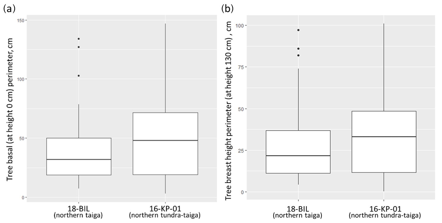
Figure A1Distribution of basal (a) and breast height (b) diameter values of trees from two focus areas: northern taiga (18-BIL) and northern tundra–taiga (16-KP-01). We also made separate models for living and dead trees as there are obvious differences in the wood densities and no needle material for dead trees. Total AGB of a tree was calculated from partial needle and wood biomass estimations.
Calculation for Pinus pumila shrub AGB
We sampled three (small, medium, big) individual pine plants on each 15 m radius sample plot that contained the species. With the following steps we calculated the AGB for each individual plant.
-
woody AGB of all small living branches (g),
where subDWSmBrB is dry weight of subsample of small-branch wood; S, M, or B is size of an individual plant; nSBr is the number of small branches; and FWSmBrB or subFWSmBrB is the fresh weight of a whole sample or subsample of small-branch wood, respectively;
-
needle AGB of all small living branches (g),
where subDWSmLB is dry weight of subsample of small-branch needles and FWSmLB or subFWSmLB is the fresh weight of a whole sample or subsample of small-branch needles, respectively;
-
woody AGB of all big living branches (g),
where subDWBiBrB is dry weight of subsample of big-branch wood; nBiBr is the number of big branches; and FWBiBrB or subFWBiBrB is the fresh weight of a whole sample or subsample of big-branch wood, respectively;
-
woody AGB of all dead branches (g),
where subDWdBrB is dry weight of subsample of dead-branch wood; ndBr is the number of dead branches; and FWdBrB or subFWdBrB is the fresh weight of a whole sample or subsample of dead-branch wood, respectively;
-
average AGB of small-living-branch wood (across the three differently sized samples; g),
-
average AGB of small-living-branch needles (g),
-
average AGB of big-living-branch wood (g),
-
average AGB of dead-branch wood (g),
-
average individual plant wood total AGB (including cone biomass; g),
where AvWoodDW is the average dry weight for only the woody part of a plant, nc is number of cones, and cB is cone biomass;
-
average volume of a shrub crown (cm3),
where SH, MH, and BH are heights of small, medium, and big plants, respectively, and Cr1 and Cr2 are two measurements of a diameter of a crown perpendicular directions;
-
average wood AGB of Pinus pumila (g m−2),
where DWAvWood is the average woody mass of a plant (m−2);
-
average needle AGB of Pinus pumila (g m−2),
where DWAvLs is the average needle mass of a plant (m−2);
-
total average AGB of Pinus pumila shrub on a 15 m radius sample plot (kg m−2),
where TDAGBPp is the total average AGB of a plant on the 15 m radius sample plot and e is cover of Pinus pumila shrubs on the 15 m radius sample plot (%).

Figure A2Allometric models, established for larch AGB: (a) for a needle biomass of a living tree in the area 16-KP-01, (b) for a wood biomass of a living tree in the area 16-KP-01, (c) for a needle biomass of a living tree in the area 18-BIL, (d) for a wood biomass of a living tree in the area 18-BIL, and (e) for a wood biomass of a dead tree in both areas.
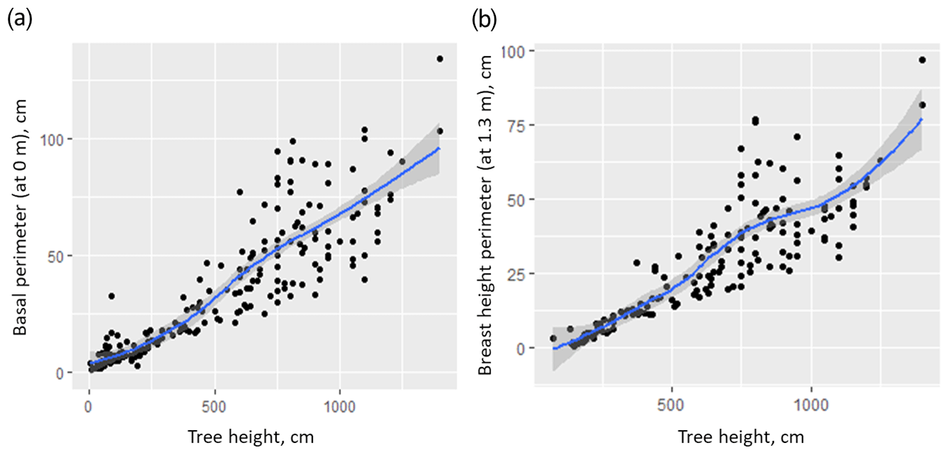
Figure A3Relationship between tree height and perimeter of the tree stem at 0 (a) and 1.3 m (b).
Calculation for Alnus fruticosa and Salix sp. shrubs AGB
We sampled three (small, medium, big) individuals as for Pinus pumila at each plot if present. Calculations are similar to those for pine but include not only big and small branches but also medium branches.
Calculation for Larix cajanderi AGB
Larix cajanderi trees were representatively subsampled at the following parts: living branches (small, medium, big), dead branches, needles from small branches, stem (ideally three tree discs at 0, 1.3, and 2.6 m heights), and cones. Total AGB of an individual tree (g) from the field survey of 2018 expedition was calculated as follows.
-
where TDAGB is total dry AGB of a tree, DBrLB is dry weight of biomass of branches and leaves, DTrB is dry weight of stem biomass.
-
where nSBr is number of small branches, SmBrB is small-branch dry biomass, SmLB is small-branch needles dry biomass, nMBr is number of medium branches, MBrB is medium-branch dry biomass, nBiBr is number of big branches, BiBrB is dry biomass of big branches, ndBR is number of dead branches, dBrB is dead-branch biomass, nc is number of cones, and cB is cone biomass.
-
where V is volume (A–B is a base of a tree stem from 0 to 130 cm; B–C is a middle part of a tree stem from 130 to 260 cm; C is a top part of a tree stem from 260 cm to the top) and TrDens is the wood density of a tree part (base, middle, or top).
-
where TrDensA is the wood density of tree disc A and TrDensB is the wood density of tree disc B.
-
where TrDensC is the wood density of a tree disc C.
-
where VAdisc is volume of a tree disc sampled at 0 cm tree stem height; BAdisc is dry weight of a tree disc sampled at 0 cm tree stem height; hAdisc is height of a tree disc sampled at 0 cm tree stem height; DAdisc is diameter of a tree disc sampled at 0 cm tree stem height; Dz is diameter of a circular hole in the central part of a disc (if present); and Crl and Crw are length and average width of a crack in the tree disc, respectively (if present). TrDensB and TrDensC are calculated by analogy with TrDensA.
-
Calculation of volume of a tree part (base, middle, or top) varies depending on presence or absence of a central hole in the tree stem.
Scenario 1. A hole in the tree disc is absent – Dz = 0:
where VA−B is the volume of a tree stem part from 0 (A) to 130 cm (B), DA is diameter of disc A, and DB is diameter of disc B.
where VC is the volume of a top part of a tree stem from 260 cm to the full height of a tree (H) and DC is the diameter of disc C.
Scenario 2. A hole in the tree disc is present only in disc A – Dz ≠ 0 (only A):
where DzA is the diameter of a central circular hole in disc A.
VC is analogous to Scenario 1.
Scenario 3. A hole in the tree disc is present in discs A and B – Dz ≠ 0 (A and B):
where DzB is the diameter of a central circular hole in disc B.
Vc is analogous to Scenario 1.
Table A1Statistics of the models for reconstructing total tree (larch) AGB.
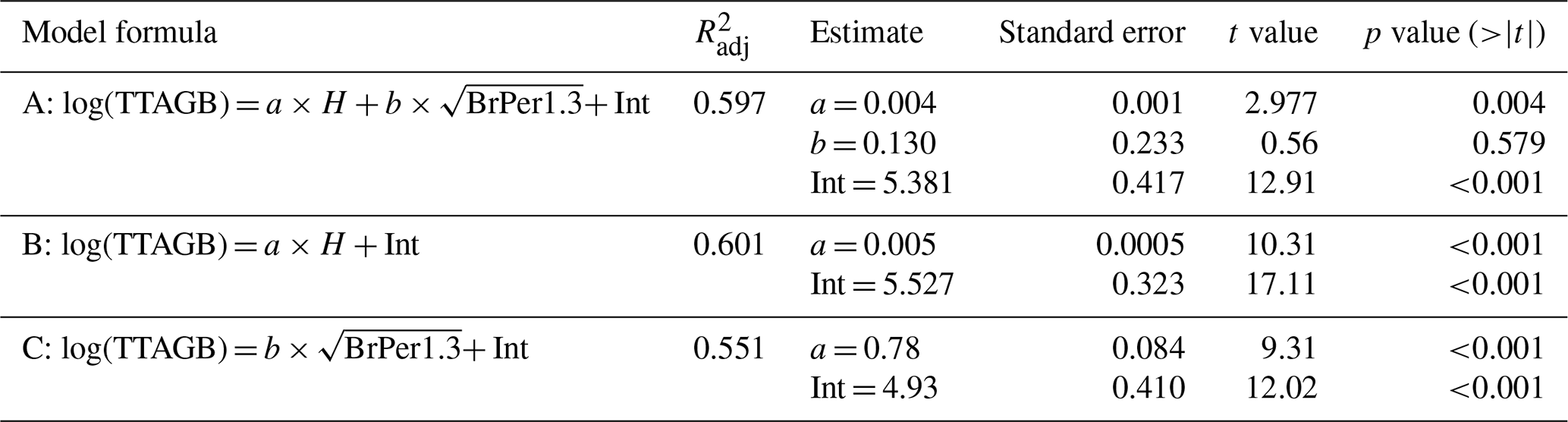
TTAGB is total tree AGB; H is tree height; BrPer1.3 is perimeter of tree stem at breast height or 1.3 m; a and b are coefficients; Int is intercept.
The next step in estimation of Larix cajanderi AGB was to estimate partial individual tree AGB for the 15 m radius sample plot, limited to tree height as a predictor (Eqs. A29–A34, Fig. A2). We did not use the tree stem diameter or perimeter for this purpose, because AGB is highly correlated with tree height (Fig. A3). We differentiated between allometric equations to estimate partial individual larch AGB from trees from two ecological regions (tundra–taiga and northern taiga).
To assess the different models for different regions we used a Wilcoxon rank sum test on measurements of tree stem perimeters. It showed significant differences between the basal perimeter and perimeter at a 1.3 m height of trees from 16-KP-01 (tundra–taiga, 178 samples) and BIL-18 (northern taiga, 74 samples) (Fig. A1). In both cases, the tree basal perimeter (p=0.007453) and tree perimeter at 1.3 m (p=0.03014) in the tundra–taiga is statistically greater than in northern taiga. Since individual trees are significantly different in the two regions, different AGB-prediction models are required for the tundra–taiga and northern taiga focus areas.
Below are the allometric equations that we established:
-
needle biomass of a living tree (area 16-KP-01; g),
where AGB is above-ground biomass and H is tree height in centimetres (Kruse et al., 2020);
-
needle biomass of a living tree (areas 18-BIL-01 and 18-BIL-02; g),
-
needle biomass of a dead tree (both regions; g),
-
wood biomass of a living tree (area 16-KP-01; g),
-
wood biomass of a living tree (area 18-BIL; g),
-
wood biomass of a dead tree (both areas; g),
Larix cajanderi AGB for a 15 m radius sample plot was calculated as follows:
where k is the number of trees on the 15 m radius sample plot, AGBn is the needle biomass of a tree, and AGBw is the woody biomass of a tree.
Tree stem perimeter and tree height are closely correlated (Fig. A3), but we tested three models for reconstructing total larch AGB to test this relationship. Table A1 shows that just using tree height gives an acceptable estimate of AGB. The highest of 0.601 is returned by the model (B) that uses only tree height as a predictor. It is slightly lower for the model (A) with both tree height and tree stem perimeter at breast height ( = 0.597), and the tree stem perimeter is an insignificant predictor. The lowest of 0.551 is for the model (C) that uses only the tree stem perimeter at breast height as a predictor of total tree AGB.
For each time stamp (2000/2001/2002 and 2016/2017) we used available Landsat acquisitions: peak summer and snow-covered (Table B1; Shevtsova et al., 2020a). We used peak-summer acquisitions to derive two Landsat spectral indices (normalised difference vegetation index (NDVI), normalised difference water index (NDWI)) and snow-covered acquisition for derivation of the normalised difference snow index (NDSI). Before calculating the indices, the Landsat data were topographically corrected. The subsets that we used for land-cover classification were cloud free and cloud shadow free. Additionally, we masked all water bodies. Landsat 8 data were transformed to Landsat 7-like data.
Landsat spectral indices NDVI, NDWI, and NDSI and projective cover of different taxa were used in the RDA, which made it possible to distinguish two RDA axes, which in total described 29 % of the variance in the projective cover through the Landsat spectral indices (Fig. B1).
Based on RDA scores we built a classification using the k-means method. We were able to derive four stable land-cover classes: (1) larch closed-canopy forest, (2) forest tundra and shrub tundra, (3) graminoid tundra, and (4) prostrate herb tundra and barren areas (Fig. B2).
Table B1Dates and short description of Landsat data used for retrieving spectral indices and further land-cover classification (in Shevtsova et al., 2020a).
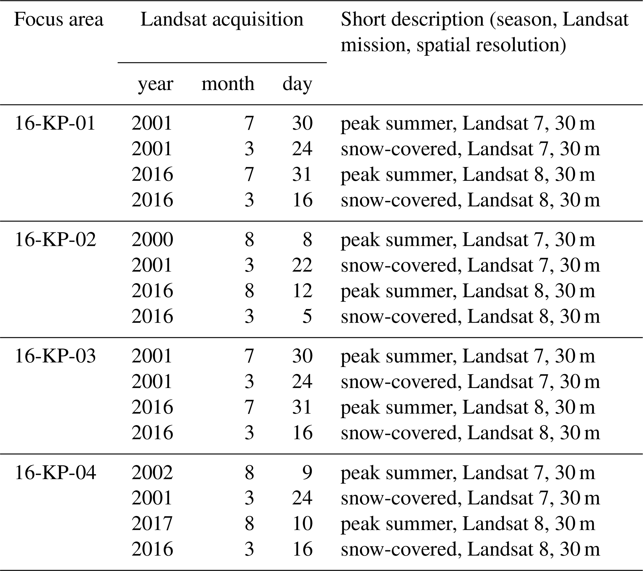
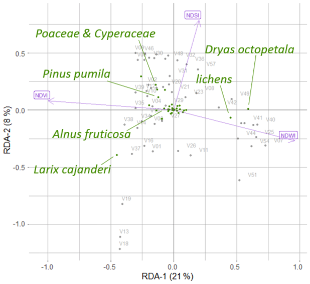
Figure B1The positions of the major taxa in the RDA space, based on foliage projective cover data of the plot taxa and Landsat spectral indices (normalised difference vegetation index (NDVI), normalised difference water index (NDWI), and normalised difference snow index (NDSI)), where V01–V58 are the 52 vegetation field sites (Shevtsova et al., 2020a).
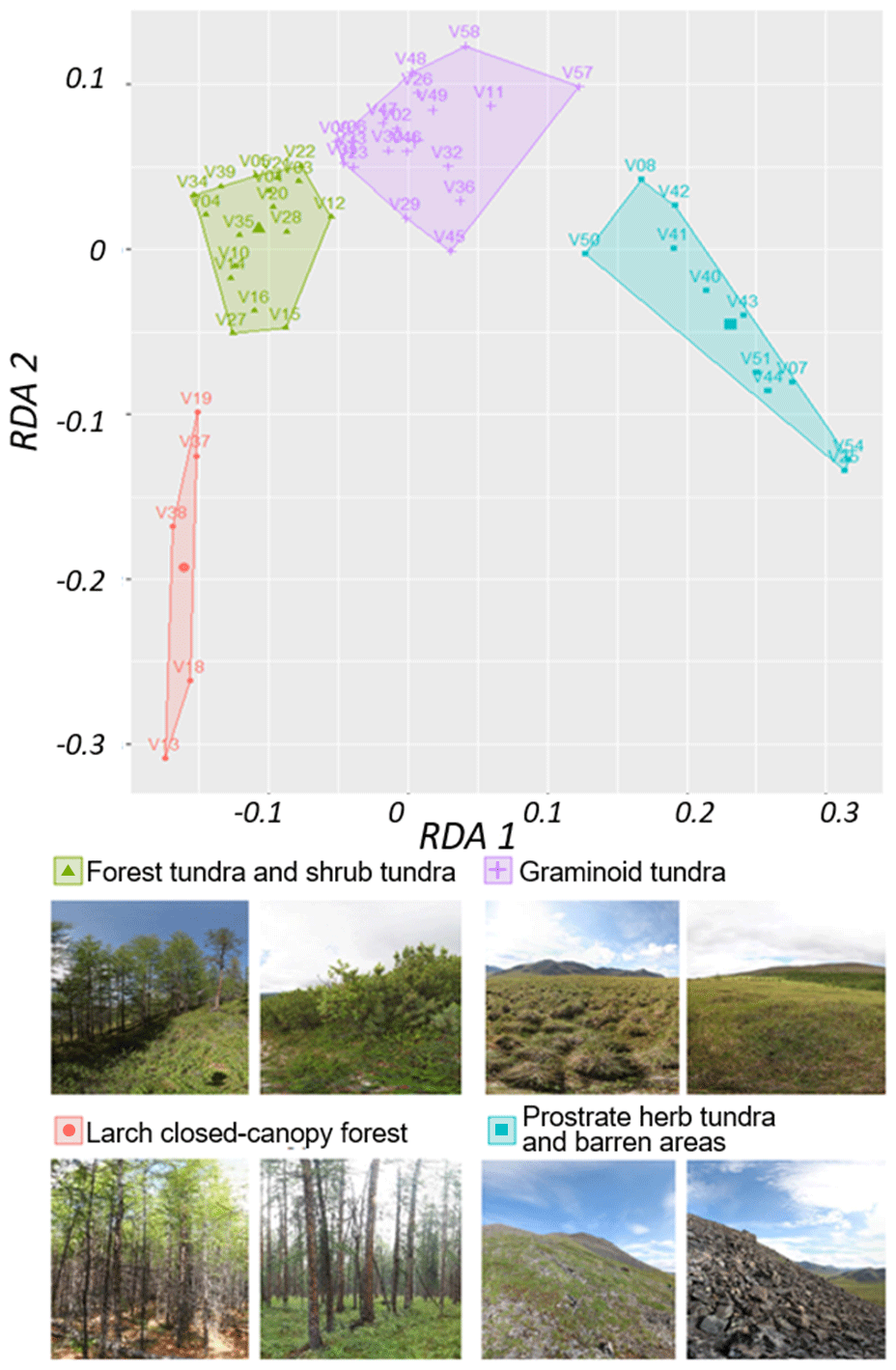
Figure B2k-means classes based on two redundancy analysis (RDA) axes using the normalised difference vegetation index (NDVI), normalised difference water index (NDWI), and normalised difference snow index (NDSI) as predictors. Images: extracts from 360×180∘ panoramic images, Stefan Kruse (figure in Shevtsova et al., 2020a).
The data that support the findings of this study are published in the PANGAEA data repository for Earth and environmental science. Data sets are accessible via the following stated links: https://doi.org/10.1594/PANGAEA.923638 (Kruse et al., 2020), https://doi.pangaea.de/10.1594/PANGAEA.923664 (Shevtsova et al., 2020b), https://doi.pangaea.de/10.1594/PANGAEA.923719 (Shevtsova et al., 2020c), and https://doi.pangaea.de/10.1594/PANGAEA.923784 (Shevtsova et al., 2020d).
IS, UH, and SK designed the study. SK, IS, UH, LS, SS, LAP, and ESZ collected the field data. SK and IS processed the field samples. BH advised on the processing of remote-sensing data. IS developed R code for processing all data used in the study, performed the formal analyses and visualisation, and prepared and edited the original manuscript. SK, UH, and BH supervised the research activity and provided critical review during manuscript preparation. UH, LP, and SK were responsible for the management and coordination of the planning and execution of the expedition project.
The authors declare that they have no conflict of interest.
This study has been supported by the German Federal Ministry of Education and Research (BMBF), which enabled the Russian–German research programme “Kohlenstoff im Permafrost” (KoPf; grant no. 03F0764A); by the Initiative and Networking Fund of the Helmholtz Association; by the ERC consolidator grant Glacial Legacy of Ulrike Herzschuh (grant no. 772852); by the Russian Foundation for Basic Research (grant no. 18-45-140053 r_a); and by the Ministry of Science and Higher Education of the Russian Federation (grant no. FSRG-2020-0019). Birgit Heim acknowledges funding by the Helmholtz Association Climate Initiative REKLIM. We thank our Russian and German colleagues from the joint German–Russian expedition Chukotka 2018 for support in the field. We would like to thank the two anonymous reviewers for proofreading and improving the paper.
This research has been supported by the German Federal Ministry of Education and Research (BMBF) the Russian–German research programme “Kohlenstoff im Permafrost” (KoPf) (grant no. 03F0764A), the ERC consolidator grant Glacial Legacy (grant no. 772852), the Russian Foundation for Basic Research (grant no. 18-45-140053 r_a), and the Ministry of Science and Higher Education of the Russian Federation (grant no. FSRG-2020-0019).
The article processing charges for this open-access publication were covered by the Alfred Wegener Institute, Helmholtz Centre for Polar and Marine Research (AWI).
This paper was edited by Frank Hagedorn and reviewed by two anonymous referees.
ACIA: Arctic Climate Impact assessment, Cambridge University Press, Cambridge, UK, 1020 pp., 2005.
Alexander, H., Mack, M., Goetz, S., Loranty, M., Beck, P., Earl, K., Zimov, S., Davydov, S., and Thompson, C.: Carbon Accumulation Patterns During Post-Fire Succession in Cajander Larch (Larix cajanderi) Forests of Siberia, Ecosystems, 15, 1065–1082, https://doi.org/10.1007/s10021-012-9567-6, 2012.
Berner, L., Jantz, P., Tape, K., and Goetz, S.: Tundra plant above-ground biomass and shrub dominance mapped across the North Slope of Alaska, Environ. Res. Lett., 13, 035002, https://doi.org/10.1088/1748-9326/aaaa9a, 2018.
Berner, L. T., Beck, P. S. A., Loranty, M. M., Alexander, H. D., Mack, M. C., and Goetz, S. J.: Cajander larch (Larix cajanderi) biomass distribution, fire regime and post-fire recovery in northeastern Siberia, Biogeosciences, 9, 3943–3959, https://doi.org/10.5194/bg-9-3943-2012, 2012.
Biskaborn, B. K., Brieger, F., Herzschuh, U., Kruse, S., Prestakova, L., Shevtsova, I., and Zakharov, E.: Glacial lake coring and treeline forest analyses at the northeastern treeline extension in Chukotka, in: Russian-German Cooperation: Expeditions to Siberia in 2018, Berichte zur Polar-und Meeresforschung [Reports on polar and marine research], edited by: Kruse, S., Bolshiyanov, D., Grigoriev, M. N., Morgenstern, A., Pestryakova, L., Tsibizov, L., and Udke, A., 734, 139–147, Bremerhaven, Alfred Wegener Institute for Polar and Marine Research, https://doi.org/10.2312/BzPM_0734_2019, 2019.
Bjarnadottir, B., Inghammar, A., Brinker, M.-M., and Sigurdsson, B.: Single tree biomass and volume functions for young Siberian larch trees (Larix sibirica) in eastern Iceland, Icelandic Agr. Sci., 20, 125–135, 2007.
Bratsch, S., Epstein, H., Buchhorn, M., Walker, D., and Landes, H.: Relationships between hyperspectral data and components of vegetation biomass in Low Arctic tundra communities at Ivotuk, Alaska, Environ. Res. Lett., 12, 025003, https://doi.org/10.1088/1748-9326/aa572e, 2017.
Bret-Harte, M. S., Mack, M. C., Goldsmith, G. R., Sloan, D. B., DeMarco, J., Shaver, G. R., Ray, P. M., Biesinger, Z., and Chapin III, F. S.: Plant functional types do not predict biomass responses to removal and fertilization in Alaskan tussock tundra, J. Ecol., 96, 713–726, https://doi.org/10.1111/j.1365-2745.2008.01378.x, 2008.
Chen, W., Li, J., Zhang, Y., Zhou, F., Koehler, K., Leblanc, S., and Wang, J.: Relating Biomass and Leaf Area Index to Non-destructive Measurements in Order to Monitor Changes in Arctic Vegetation, Arctic, 62, 281–294, https://doi.org/10.14430/arctic148, 2009.
Dong, L., Zhang, Y., Zhang, Z., Xie, L., and Li, F.: Comparison of Tree Biomass Modeling Approaches for Larch (Larix olgensis Henry) Trees in Northeast China, Forests, 11, 202, https://doi.org/10.3390/f11020202, 2020.
Epstein, H., Walker, D., Raynolds, M., Jia, G., and Kelley, A.: Phytomass patterns across a temperature gradient of the North American arctic tundra, J. Geophys. Res., 113, G03S02, https://doi.org/10.1029/2007jg000555, 2008.
Epstein, H., Raynolds, M., Walker, D., Bhatt, U., Tucker, C., and Pinzon, J.: Dynamics of aboveground phytomass of the circumpolar Arctic tundra during the past three decades, Environ. Res. Lett., 7, 015506, https://doi.org/10.1088/1748-9326/7/1/015506, 2012.
Fassnacht, F. E., Hartig, F., Latifi, H., Berger, C., Hernández, J., Corvalán, P., and Koch, B.: Importance of sample size, data type and prediction method for remote sensing-based estimations of aboveground forest biomass, Remote Sens. Environ.t, 154, 102–114, https://doi.org/10.1016/j.rse.2014.07.028, 2014.
Grigoryev, A. A.: Subarktyka [Subarctic], Publ. Acad. Sci. SSSR., Moscow-Leningrad, 1946 (in Russian).
Hijmans, R. J.: Raster: Geographic Data Analysis and Modeling, R package version 2.6-7, available at: https://CRAN.R-project.org/package=raster (last access: 22 February 2021), 2017.
Hobbie, S. and Chapin, F.: The Response of Tundra Plant Biomass, Aboveground Production, Nitrogen, and CO2 Flux to Experimental Warming, Ecology, 79, 1526, https://doi.org/10.2307/176774, 1998.
Hudson, J. M. G. and Henry, G. H. R.: Increased plant biomass in a High Arctic heath community from 1981 to 2008, Ecology, 90, 2657–2663, https://doi.org/10.1890/09-0102.1, 2009.
IPCC: Global Warming of 1.5 ∘C, An IPCC Special Report on the impacts of global warming of 1.5 ∘C above pre-industrial levels and related global greenhouse gas emission pathways, in: the context of strengthening the global response to the threat of climate change, sustainable development, and efforts to eradicate poverty, edited by: Masson-Delmotte, V., Zhai, P., Pörtner, H. O., Roberts, D., Skea, J., Shukla,P. R., Pirani, A., Moufouma-Okia, W., Péan, C., Pidcock, R., Connors, S., Matthews, J. B. R., Chen, Y., Zhou, X., Gomis, M. I., Lonnoy, E., Maycock, T., Tignor, M., and Waterfield, T., in press, 2018.
Jobbágy, E. and Jackson, R.: The vertical distribution of soil organic carbon and its relation to climate and vegetation, Ecol. Appl., 10, 423–436, https://doi.org/10.1890/1051-0761(2000)010[0423:tvdoso]2.0.co;2, 2000.
Kassambara A. and Mundt F.: factoextra: Extract and Visualize the Results of Multivariate Data Analyses, R package version 1.0.5.999, available at: http://www.sthda.com/english/rpkgs/factoextra (last access: 22 February 2021), 2017.
Kruse, S., Herzschuh, U., Schulte, L., Stuenzi, S. M., Brieger, F., Zakharov, E. S., and Pestryakova, L. A.: Forest inventories on circular plots on the expedition Chukotka 2018, NE Russia, PANGAEA [Dataset], https://doi.org/10.1594/PANGAEA.923638, 2020.
Legendre, P. and Legendre, L.: Numerical Ecology, 3rd Edn., Elsevier, Amsterdam, the Netherlands, 2012.
Loranty, M. M., Davydov, S. P., Kropp, H., Alexander, H. D., Mack, M. C., Natali, S. M., and Zimov, N. S.: Vegetation Indices Do Not Capture Forest Cover Variation in Upland Siberian Larch Forests, Remote Sens., 10, 1686, https://doi.org/10.3390/rs10111686, 2018.
Maslov, M. N., Kopeina, E. I., Zudkin, A. G., Korolevam N. E., Shulakovm A. A., Onipchenkom V. G., and Makarovm M. I.: Stocks of phytomass and organic carbon in tundra ecosystems of northern Fennoscandia, Moscow Univ. Soil Sci. Bull. 71, 113–119, https://doi.org/10.3103/S0147687416030042, 2016.
McGuire A. D., Anderson L. G., Christensen T. R., Dallimore S., Guo L., Hayes D. J., Heimann M., Lorenson T. D., Macdonald R. W., and Roulet N.: Sensitivity of the carbon cycle in the Arctic to climate change, Ecol. Monogr., 79 523–55, https://doi.org/10.1890/08-2025.1, 2009.
Oksanen, J., Blanchet, F. G., Friendly, M., Kindt, R., Legendre, P., McGlinn, D., Minchin, P. R., O'Hara, R. B., Simpson, G. L, Solymos, P., Stevens, M. H. H., Szoecs, E., and Wagner H.: vegan: Community Ecology Package, R package version 2.5-4, available at: https://CRAN.R-project.org/package=vegan (last access: 22 February 2021), 2019.
Pattison, R. R., Jorgenson, J. C., Raynolds, M. K., and Welker J. M.: Trends in NDVI and Tundra Community Composition in the Arctic of NE Alaska between 1984 and 2009, Ecosystems, 18, 707–719, https://doi.org/10.1007/s10021-015-9858-9, 2015.
Pebesma, E. J. and Bivand, R. S.: Classes and methods for spatial data in R, R News, 5, 9–13, https://cran.r-project.org/doc/Rnews/ (last access: 22 February 2021), 2005.
Pettorelli, N., Vik, J. O., Mysterud, A., Gaillard, J.-M., Tucker, C. J., and Stenseth, N. C.: Using the satellite-derived NDVI to assess ecological responses to environmental change Trends in Ecology and Evolution, 20, 503–510, https://doi.org/10.1016/j.tree.2005.05.011, 2005.
R Core Team: R: A language and environment for statistical computing, R Foundation for Statistical Computing, Vienna, Austria, available at: https://www.R-project.org/ (last access: 22 February 2021), 2017.
Räsänen, A., Juutinen, S., Aurela, M., and Virtanen, T.: Predicting aboveground biomass in Arctic landscapes using very high spatial resolution satellite imagery and field sampling, Int. J. Remote Sens., 40, 1175–1199, https://doi.org/10.1080/01431161.2018.1524176, 2018.
Raynolds, M., Walker, D., Epstein, H., Pinzon, J., and Tucker, C.: A new estimate of tundra-biome phytomass from trans-Arctic field data and AVHRR NDVI, Remote Sens. Lett., 3, 403–411, https://doi.org/10.1080/01431161.2011.609188, 2011.
Santoro, M. and Cartus, O.: ESA Biomass Climate Change Initiative (Biomass_cci): Global datasets of forest above-ground biomass for the year 2017, v1, Centre for Environmental Data Analysis [Dataset], https://doi.org/10.5285/bedc59f37c9545c981a839eb552e4084, 2019.
Shaver, G. and Chapin, F.: Production: Biomass Relationships and Element Cycling in Contrasting Arctic Vegetation Types, Ecol. Monogr., 61, 1–31, https://doi.org/10.2307/1942997, 1991.
Shevtsova, I., Heim, B., Kruse, S., Schröder, J., Troeva, E., Pestryakova, L., Zakharov, E., and Herzschuh, U.: Strong shrub expansion in tundra-taiga, tree infilling in taiga and stable tundra in central Chukotka (north-eastern Siberia) between 2000 and 2017, Environ. Res. Lett., 15, 085006, https://doi.org/10.1088/1748-9326/ab9059, 2020a.
Shevtsova, I., Kruse, S., Herzschuh, U., Schulte, L., Brieger, F., Stuenzi, S. M., Heim, B., Troeva, E. I., Pestryakova, L. A., and Zakharov, E. S.: Foliage projective cover of 40 vegetation sites of central Chukotka from 2018, PANGAEA [Dataset], https://doi.pangaea.de/10.1594/PANGAEA.923664, 2020b.
Shevtsova, I., Kruse, S., Herzschuh, U., Schulte, L., Brieger, F., Stuenzi, S. M., Heim, B., Troeva, E. I., Pestryakova, L. A., and Zakharov, E. S.: Total above-ground biomass of 39 vegetation sites of central Chukotka from 2018, PANGAEA [Dataset], https://doi.pangaea.de/10.1594/PANGAEA.923719, 2020c.
Shevtsova, I., Kruse, S., Herzschuh, U., Schulte, L., Brieger, F., Stuenzi, S. M., Heim, B., Troeva, E. I., Pestryakova, L. A., and Zakharov, E. S.: Individual tree and tall shrub partial above-ground biomass of central Chukotka in 2018, PANGAEA [Dataset], https://doi.pangaea.de/10.1594/PANGAEA.923784, 2020d.
Vankoughnett, M. R. and Grogan, P: Plant production and nitrogen accumulation above- and belowground in low and tall birch tundra communities: the influence of snow and litter, Plant Soil, 408, 195–210, https://doi.org/10.1007/s11104-016-2921-2, 2016.
Walker, D. A. and Raynolds, M. K.: Circumpolar Arctic Vegetation, Geobotanical, Physiographic Maps, 1982–2003, ORNL DAAC, Oak Ridge, Tennessee, USA, https://doi.org/10.3334/ORNLDAAC/1323, 2018.
Webb, E. E., Heard, K., Natali, S. M., Bunn, A. G., Alexander, H. D., Berner, L. T., Kholodov, A., Loranty, M. M., Schade, J. D., Spektor, V., and Zimov, N.: Variability in above- and belowground carbon stocks in a Siberian larch watershed, Biogeosciences, 14, 4279–4294, https://doi.org/10.5194/bg-14-4279-2017, 2017.
Wickham, H.: ggplot2: Elegant Graphics for Data Analysis, Springer-Verlag, New York, 2016.
Wood, S. N.: Fast stable restricted maximum likelihood and marginal likelihood estimation of semiparametric generalized linear models, J. Roy. Stat. Soc. B, 73, 3–36, 2011.
- Abstract
- Introduction
- Materials and methods
- Results
- Discussion
- Conclusions
- Appendix A: Sampling and above-ground biomass (AGB) calculation protocol for field data
- Appendix B: Landsat satellite data and statistical analysis as preparation for the AGB upscaling
- Data availability
- Author contributions
- Competing interests
- Acknowledgements
- Financial support
- Review statement
- References