the Creative Commons Attribution 4.0 License.
the Creative Commons Attribution 4.0 License.
 | 22 Jun 2021
Reviews and syntheses: Gaining insights into evapotranspiration partitioning with novel isotopic monitoring methods
Maria Quade
Nicolas Brüggemann
Alexander Graf
Harry Vereecken
Maren Dubbert
Disentangling ecosystem evapotranspiration (ET) into evaporation (E) and transpiration (T) is of high relevance for a wide range of applications, from land surface modelling to policymaking. Identifying and analysing the determinants of the ratio of T to ET () for various land covers and uses, especially in view of climate change with an increased frequency of extreme events (e.g. heatwaves and floods), is prerequisite for forecasting the hydroclimate of the future and tackling present issues, such as agricultural and irrigation practices.
One partitioning method consists of determining the water stable isotopic compositions of ET, E, and T (δET, δE, and δE, respectively) from the water retrieved from the atmosphere, the soil, and the plant vascular tissues. The present work emphasizes the challenges this particular method faces (e.g. the spatial and temporal representativeness of the estimates, the limitations of the models used, and the sensitivities to their driving parameters) and the progress that needs to be made in light of the recent methodological developments. As our review is intended for a broader audience beyond the isotopic ecohydrological and micrometeorological communities, it also attempts to provide a thorough review of the ensemble of techniques used for determining δET, δE, and δE and solving the partitioning equation for .
From the current state of research, we conclude that the most promising way forward to ET partitioning and capturing the subdaily dynamics of is by making use of non-destructive online monitoring techniques of the stable isotopic composition of soil and xylem water. Effort should continue towards the application of the eddy covariance technique for high-frequency determination of δET at the field scale as well as the concomitant determination of δET, δE, and δE at high vertical resolution with field-deployable lift systems.
Please read the corrigendum first before continuing.
-
Notice on corrigendum
The requested paper has a corresponding corrigendum published. Please read the corrigendum first before downloading the article.
-
Article
(4042 KB)
-
The requested paper has a corresponding corrigendum published. Please read the corrigendum first before downloading the article.


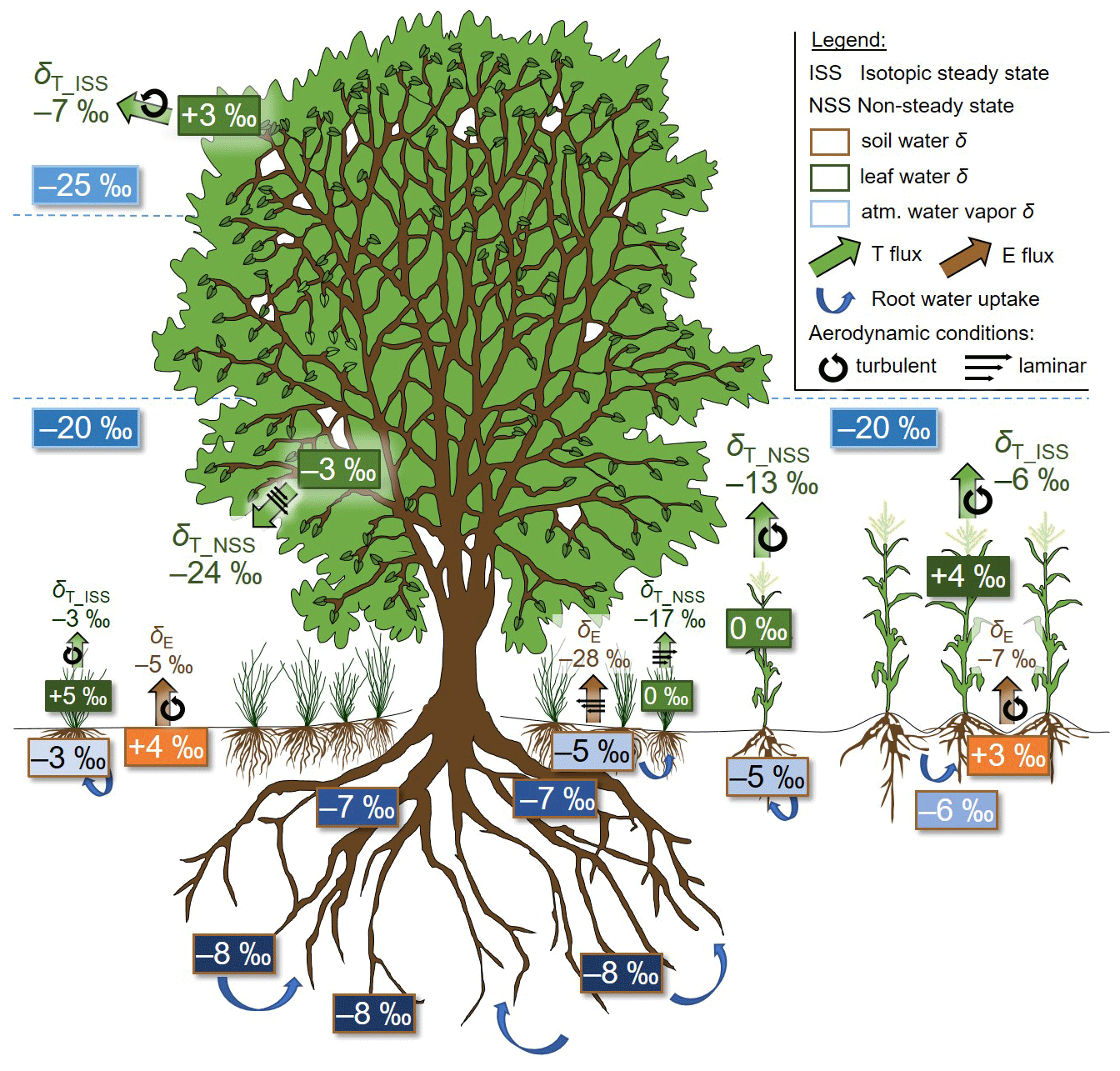
Figure 1Conceptual drawing reporting the sources of differences in (synthetic) values between the (exemplary oxygen) isotopic compositions of evaporation (δE, ‰) and transpiration (δE, ‰) in an agroforestry context, namely (i) the type of vegetation and root development (tree vs. maize crop vs. grass layer); (ii) the prevalence of isotopic-steady-state (ISS) or non-steady-state (NSS) conditions for leaf water; and (iii) the environmental conditions acting on fluxes, i.e. soil water and atmospheric water vapour isotopic composition profiles, and leaf water isotopic composition (values displayed in boxes outlined in brown, blue, and green). δE and NSS δE values were calculated with the Craig and Gordon (1965) model assuming laminar-flow conditions (designated by the three superimposed arrows) under the pictured tree and within its canopy and fully turbulent conditions (designated by a circular arrow) elsewhere (e.g. at the top of the tree canopy, above the maize crop for δE, and in its interrow space for δE).
A pivotal parameter in landscape hydrology and ecology is the transpiration (T) to evapotranspiration (ET) ratio () (see the reviews of Kool et al., 2014; Anderson et al., 2017; Stoy et al., 2019). Isolating the T flux in ET is of utmost importance for a wide range of applications because of its link to plant water uptake, for e.g. optimizing irrigation practices (Skaggs et al., 2010), tackling ecological questions in water-limited ecosystems (Rothfuss and Javaux, 2017), or a better representation of the relations between the carbon and water cycles in climate models (Humphrey et al., 2018; Ito and Inatomi, 2012). At the global scale, the uncertainty of the estimate remains high; it has been estimated to range from 13 % to 90 %, depending on the source and type of data (e.g. satellite- or isotopic-based) and method (modelling or data reanalysis) (Lawrence et al., 2007; Alton et al., 2009; Jasechko et al., 2013; Wang et al., 2014; Wei et al., 2017). Ultimately, this conditions the ability of land surface models to provide sensitivity of the overall ET flux to changes in precipitation and land cover (Wang and Dickinson, 2012).
Spatial and temporal variability add even more uncertainty to our knowledge about at the local scale, which is a prerequisite for a meaningful use of such estimates for any of the practical and scientific questions mentioned above. Partitioning ET into the raw components E and T at the field and subdaily spatiotemporal scales is generally performed by an ensemble of partitioning methods, which can be divided into instrumental approaches and correlation-based modelling approaches (Scanlon and Kustas, 2010). The former approach includes e.g. the eddy covariance (EC) technique (Baldocchi, 2014; Reichstein et al., 2005), soil flux chamber measurements (Raz-Yaseef et al., 2010; Lu et al., 2017), micro-lysimeter measurements (Kelliher et al., 1992), or atmospheric-profile measurements (Ney and Graf, 2018).
Another instrumental method to partition ET is based on the analysis of its hydrogen or oxygen isotopic composition, i.e. the water vapour atom ratio in rare (2H or 18O) and abundant (1H or 16O) stable isotopes and expressed on the international “delta” (δ) scale (Dubbert and Werner, 2019). The method utilizes the natural discrepancies in isotopic composition of the ecosystem evaporation (δE) and transpiration (δE) fluxes. The difference of δE − δE originates primarily from thermodynamic and kinetic fractionation during phase change and transport processes undergone by water evaporating from soil on the one hand and water extracted by a root system and transpired by the canopy on the other hand. The observed discrimination against stable isotopologues along the soil–plant–atmosphere water path can be conceptualized twofold, i.e. phase-change- and diffusion-driven, and quantified by the so-called equilibrium and kinetic fractionations, respectively, for which we will later review the physically based expressions. The term (δE − δE) is also determined by (see Fig. 1)
- i.
the difference in boundary conditions acting on E and T, i.e. the δ value of soil water at the evaporating front (EF) and that of the leaf water at the transpiration site and of the atmospheric water vapour;
- ii.
the prevalence (or non-prevalence) of isotopic steady state (ISS) for transpiration, i.e. whether δE is independent of time (Farquhar and Cernusak, 2005; Dubbert et al., 2014a) (see Sect. 3 for a detailed description of ISS; note that the ISS assumption is generally not made for evaporation flux, but see Rothfuss et al., 2010, for an exception).
The spatiotemporal variabilities of these factors and the complexity of their interactions may result in significant heterogeneous distributions of both δE and δE in the field (Fig. 1). Importantly and as reflected by the reviewed isotopic literature (see Sect. 2), E in this context does not include canopy interception and dew evaporation, which are known to be associated with isotopic effects (Allen et al., 2017; Zheng et al., 2019). Theses fluxes can be of significant magnitude, depending on the scale of interest (Good et al., 2015; Allen et al., 2017). The fraction is obtained by inverting the isotopic mass balance equation (Yakir and Sternberg, 2000):
Equation (1) highlights how the isotopic partitioning methodology differs from other instrumental approaches, such as those based on a combination of different techniques (e.g. lysimeter and EC measurements): it solely relies on measurements and/or analytical modelling of the stable isotopic compositions of the components ET, E, and T. Behind this apparent simplicity and the problem of (e.g. spatial) representativeness highlighted in Fig. 1 put aside, the isotopic partitioning methodology is limited in its application in different ways, such as the inability – until recently – to provide continuous (i.e. non-destructive) δE, δE, and δET assessments. Part of these limitations were overcome with the availability of field-deployable laser-based spectrometers. These instruments allow for long-term monitoring of soil water vapour and plant transpiration isotopic compositions when combined with gas-permeable membrane or tubing technology (Beyer et al., 2020).
A variety of different methods exist to measure or estimate δE, δE, and δET. The central aim of this study is to identify from the literature the challenges the ensemble of isotopic methods currently face and how they should progress in the future (Sect. 3). Particularly, the abovementioned emerging monitoring methods are reviewed for the specific purpose of ET partitioning. As such, our work differs from those of Wang and Yakir (2000), Yakir and Sternberg (2000), Xiao et al. (2018), and Sun et al. (2019). Note also that this study will not focus on differences in as estimated by the abovementioned traditional methods on the one hand and by the isotopic methods on the other; this has been extensively reported by e.g. Sutanto et al. (2014). In addition and for non-specialist readers, we thoroughly review the underlying concepts and techniques involved in the determination of δE, δE, and δET. In order to highlight the important progresses made over the past 30 years, we also give a literature overview (Sect. 2). Finally, Sect. 5 presents a summary of our own suggestion for improvement as well as of the possible ways forward for the isotopic partitioning community.
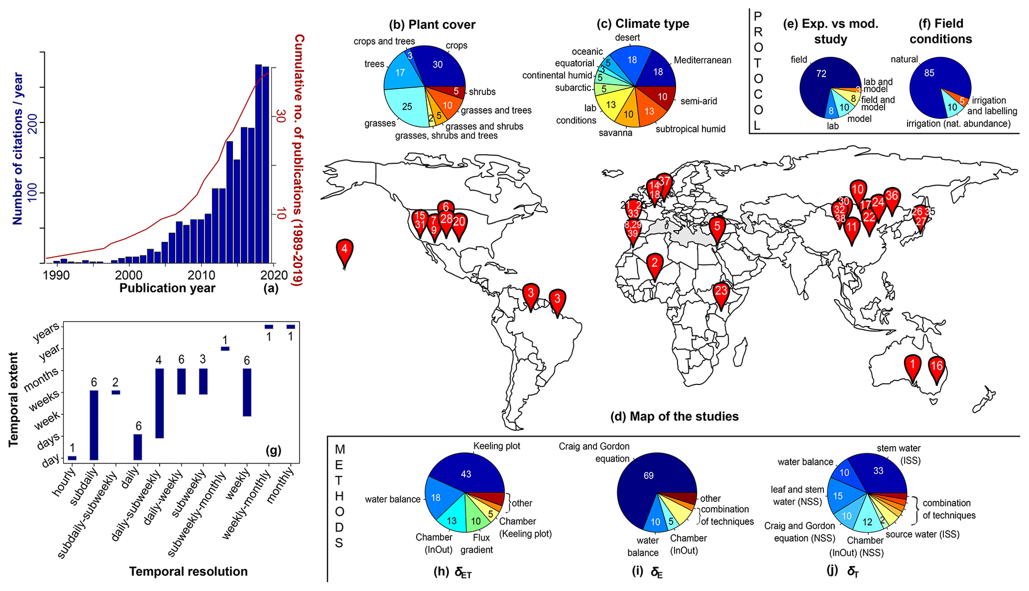
Figure 2Graphical summary of the reviewed literature. (a) Evolution of the number of citations per year (blue bars) and cumulative number of publications (1989–2020, red line). (b) Temporal resolution vs. extent of the estimate of the transpiration-to-evapotranspiration ratio (). Numbers above or below the histograms refer to the number of studies working at a given temporal resolution. (c, d) Listing of the different plant cover and climate types with proportions (white label) expressed in percentage and (g) map locating each study (with reference number 1–39 with a white label; see Table A1). (e, f) Proportions of field vs. modelling studies and prevailing experimental conditions (as natural precipitation or irrigation or else as labelling studies). (h–j) Listing and proportions of methods for determination of δET, δE, and δE.
A total of 39 studies were found by entering the search terms ((“evapotranspiration” or “transpiration” or “evaporation”) and partition* and isotop*) into the ISI (Institute for Scientific Information) Web of Science search engine (http://www.webofknowledge.com/, last access: 15 February 2021). The reader
will find a graphical summary in Fig. 2 as well as a detailed description for each of the entries in Table A1 of Appendix A. On average, approximately 1.3 (2.4) partitioning studies were published each year over the period 1989–2007
(2008–2020) with an average annual citation rate of 12 (143) (Fig. 2a).
To the authors' knowledge, the first scientific article reporting on the possibility to partition ET on basis of the differences in isotopic composition of ecosystem ET, soil evaporation, and plant transpiration was that of Bariac et al. (1987). An attempt to use this possibility was made in the study of Walker and Brunel (1990) (Table A1) but remained, according to the authors, not conclusive; 10 years later, Jean-Pierre Brunel and his colleagues could provide the first water-stable-isotope-derived estimation of the relative importance to ET of the transpiration of the tropical and water-stress-resistant plant Guiera senegalensis (Brunel et al., 1997), which was noticeably low (approx. 20 %). In the meantime, Moreira et al. (1997) applied the so-called “Keeling plot” technique (Keeling, 1958) (see Sect. 3.1) for determination of the isotopic composition of ET for the specific purpose of partitioning. The isotopic compositions of soil E and plant T at two sites (one pasture and one forest) in the Amazon basin were inferred by using the atmospheric part of the Craig and Gordon (1965) model (see Sect. 3.2) and by assuming steady-state transpiration flux (see Sect. 3.3), respectively. The authors could provide evidence of the strong prevalence of T in the ET budget. In a hybrid work coupling a review of the state of the art with field measurements, Wang and Yakir (2000) concluded on the predominance of T flux in a wheat field located in the Negev region, Israel (i.e. > 96.5 %).
As represented in Fig. 1, partitioning ET may be significantly complicated in cases of mixed vegetation covers. A few studies focused on estimating the ratio of the vegetation type or strata-specific transpiration to evapotranspiration. Yepez et al. (2003) applied the Keeling plot technique specifically to two distinct ecosystem layers of a savanna woodland in southern Arizona, USA, i.e. the understorey dominated by the Sporobolus wrightii C4 grass and the canopy populated by the mesquite tree Prosopis velutina. By doing this, they could capture the isotopic composition of ET representative of each of the two ecosystem layers. In order to partition ET, the authors computed the isotopic composition of the whole ecosystem T as a composite function of the isotopic compositions of grass and tree T fluxes. Finally, it was determined that grass and tree T amounted to 15 % and 75 % of total ET. Xu et al. (2008) investigated the discrepancies between assessments from either δ2H or δ18O data collected in a subalpine shrubland (Balang Mountain, China). They could differentiate between tree (Quercus aquifolioides) and understorey (e.g. Cystopteris montana) contributions to ET by using the multi-source mixing model IsoSource (Phillips and Gregg, 2003). In an open cork-oak (Quercus suber L.) savanna, Dubbert et al. (2014b) investigated the impact of the understorey vegetation (annual grass and forbs) on the total ecosystem water budget. They could discriminate between T of trees and grass and highlighted the stability of the former throughout the year and the strong decrease of the latter during the summer. Piayda et al. (2017) differentiated between open and shaded portions of the same experimental site and found ranging from 9 % to 59 % and from 17 % to 66 %, respectively. Zhang et al. (2018) investigated a marsh wetland in China and found out that the two dominant species (Scirpus triqueter and the invasive Phragmites australis) contributed equally (20 %) to ET flux.
A number of authors either investigated the impact of irrigation on the partitioning of ET or relied on irrigation pulses, i.e. applied volumes of isotopically enriched or depleted water (with respect to local irrigation water) to the soil. By doing this, they could reduce the uncertainty of the estimates by artificially enhancing the difference between δE and δE. In a study conducted in a semi-arid environmental setting (Marrakesh, Morocco), Williams et al. (2004) observed that irrigation enhanced soil E of an olive orchard (Olea europaea L.). Midday average decreased from approx. 100 % (determined prior irrigation) to 69 %–86 % (computed over the 5 d period after irrigation). Yepez et al. (2005) used large gas exchange chambers either positioned on bare-soil plots or sparsely vegetated areas of a semi-arid grassland in Arizona, USA. They determined with the Keeling plot technique the isotopic composition of E and ET following an irrigation pulse. This is, to the authors' knowledge, the first use of a closed chamber system in the context of ET partitioning where T is the single source of the change in air moisture concentration. In contrast to the previous partitioning studies, Yepez et al. (2005) determined the isotopic composition of the non-steady-state (NSS) T flux on the basis of plant physiological and micrometeorological measurements using the formulation of Farquhar and Cernusak (2005) (see also for later examples Sun et al., 2014; Hu et al., 2014). The authors finally calculated values ranging between 35 % and 43 % the first 3 d after irrigation, and these decreased to 22 % after 1 week. Aouade et al. (2016) found a decreasing diurnal (i.e. morning vs. afternoon) amplitude of in a winter wheat field in Morocco under wet conditions after flood irrigation (soil water content value of approx. 0.35 m3 m−3) and the opposite under dry conditions (soil water content value of approx. 0.15 m3 m−3). Aouade et al. (2020) compared the results for dry conditions of Aouade et al. (2016) to independent assessments using the Interaction between Soil, Biosphere, and Atmosphere (ISBA) model (Masson et al., 2013) and found that they were within the same range (73 %–89 %). In another study, Good et al. (2014) found on average a value of 30 (± 5) % for in a grassland site during the first 15 d following a 30 mm isotopically enriched irrigation event. Finally, Lu et al. (2017) focused on the efficiency of irrigation strategies in southern California (USA). They documented that the investigated field of Sorghum bicolor was responsible for 46 % of water consumption following the irrigation event.
Hsieh et al. (1998), Ferretti et al. (2003), Wenninger et al. (2010), and Sutanto et al. (2012) obtained values by the closing of a common water isotope mass balance equation. For this, the authors made a series of simplifying hypotheses: atmospheric water vapour is in thermodynamic equilibrium with soil water, and the isotopic composition of T is the amount-weighted average of the isotopic compositions of precipitation and soil water. Ferretti et al. (2003) obtained values ranging between 10 % and 60 %, depending on the growing season, in a semi-arid grass steppe, while Hsieh et al. (1998) estimated to span from 14 % to 71 % as annual rainfall increased along two sampling transects in Hawaii. Wenninger et al. (2010) and Sutanto et al. (2012) applied the isotope mass balance equation in similar semi-controlled experimental setups equipped with soil liquid water (Rhizon) samplers. In their framework, the destructive sampling of soil to retrieve the isotopic composition of soil E was not needed, while a number of simplified hypotheses had to be made regarding T. Wenninger et al. (2010) simulated a value of 70 % for teff (Eragrostis tef) during the course of their experiment. Sutanto et al. (2012) found a comparable value for a grass cover ( = 87 %). In both of these studies, the isotopic partitioning results were confronted with additional (e.g. micrometeorological) measurements and independent models such as HYDRUS-1D (Simunek and van Genuchten, 2008).
Isotope-enabled, physically based, and numerically solved soil–vegetation–atmosphere transfer (SVAT) models were also tested against data collected in both laboratory and field setups. In the study of Rothfuss et al. (2012), of a 0.2 m2 surface area monolith was simulated with the SiSPAT-Isotope model (Simple Soil–Plant–Atmosphere Transfer; Braud et al., 2005) at five selected dates under strictly controlled conditions in a climate chamber along the development of a tall fescue cover (Festuca arundinacea). was determined to increase from 6 % (16 d after sowing) to 95 % (43 d after sowing); 1 year earlier, Haverd et al. (2011) used another isotopically SVAT model, Soil–Litter–Iso (Haverd and Cuntz, 2010), using data from a field experiment (eucalyptus forest, southeastern Australia) in a similar framework, i.e. by running a multi-objective calibration to estimate a given set of model parameters. However, in contrast to Rothfuss et al. (2012), they could show that the added information provided by the isotopic data (δ2H) was not effective in better constraining the model for determination of (in their case equal to 85 ± 2 %). Another simulation study was published by Wang et al. (2015), where a physically based model solving the energy and water balance in the soil–plant–atmosphere continuum (Wang and Yamanaka, 2014) was coupled to an isotopic module accounting for fractionation processes during E and T. Wang et al. (2015) simulated of a temperate grassland to spread over a wide range of values (i.e. 2 %–99 %) during the course of a 190 d long experiment. Wei et al. (2018) used a similar modelling framework as in Wang et al. (2015) and found that the 3-month ET-weighted values were equal to 74, 93, and 81 % for three different crops, i.e. rice, corn, and wheat, respectively, grown in temperate (rice, Japan) and semi-arid monsoonal (corn and wheat, China) environmental conditions.
Wang et al. (2010, 2013) published the first ET partitioning studies where water vapour hydrogen and oxygen isotopic compositions were measured online with an infrared laser spectrometer. Using closed gas exchange chambers, they determined by mass balance the isotopic compositions of E, T, and ET in a non-destructive way. This allowed the authors not to rely on either (i) making the assumption of T at ISS for partitioning ET fluxes or (ii) modelling the isotopic composition of T at NSS (see Sect. 3.3). Wang et al. (2010) calculated values for the mesquite tree (Prosopis chilensis) grown under controlled conditions (Biosphere 2 facility, Arizona, USA; see for details Barron-Gafford et al., 2007), ranging from 61 % to 83 % at 25 % and 100 % woody cover, respectively. Wang et al. (2013) compared values (65 %–77 % vs. 83 %–86 %) computed from control vs. warming plots, taking advantage of a long-term grassland multiple-factor climate control experiment in Oklahoma, USA.
The quantification of the overall uncertainty associated with isotope-derived estimates has been the focus of several studies. Other studies focused on the sensitivity of to different environmental (e.g. isotopic) factors. Good et al. (2014) studied for instance the uncertainty of the values obtained at their grassland site as a function of the uncertainty linked with the estimate of δET obtained with the Keeling plot technique (according to Good et al., 2012). Bijoor et al. (2011) highlighted the high uncertainty of their isotope estimates (i.e. standard error value > 37 %). Xu et al. (2008) and Yepez et al. (2005) calculated the uncertainties linked with determination of with the IsoError software (Phillips and Gregg, 2001). Dubbert et al. (2013) quantified the sensitivity of the partitioning of ET to a number of factors (e.g. value of the kinetic fractionation factor and assumption of steady-state T) during a field experiment in central Portugal. They also compared direct measurements of the isotopic composition of E (with gas exchange chambers coupled to a laser spectrometer) to simulations with the Craig and Gordon (1965) model. Similar to Rothfuss et al. (2010, 2012), the authors underlined the need to complement isotopic measurement with micrometeorological and physiological observations. Hu et al. (2014) determined a mean value of 83 % in a semi-arid shrubland in China dominated by Stipa krylovii and Artemisia frigida. They tested for the first time the so-called flux gradient approach (Lee et al., 2007; see Sect. 3.1) for determination of δET. The authors argued that, in their case, the uncertainty of the δET estimates had the strongest effect on uncertainty. Also Wei et al. (2015) found that the greatest source of uncertainty of of a rice paddy field was linked to the determination of δET, this time using the Keeling plot technique. They could further express as an exponential function of leaf area index (LAI) (i.e. = 67 ⋅ LAI0.25, expressed in %) at the seasonal scale. Wu et al. (2017) found slightly different parameters of the same LAI model (71 ⋅ LAI0.14) for a maize crop grown under semi-arid conditions (Gansu Province, China).
Among the studies listed in Table A1, a few complemented their isotopic methods with traditional instrumental approaches, such as EC, soil flux chambers, and lysimeters, and investigated the goodness of fit between the isotopic and non-isotopic values. Sutanto et al. (2014) reported from the literature generally higher isotope-derived (> 70 %) values than those of the traditional approaches for comparable land cover types. However, at experimental sites combining both type of measurements, Sutanto et al. (2014) underlined a fair agreement between both approaches. Bijoor et al. (2011) investigated the partitioning of ET in a freshwater marsh dominated by Typha latifolia in California, USA. They found a good agreement between values estimated on the one hand from isotopic analysis and from micrometeorological (e.g. EC) measurements on the other. Berkelhammer et al. (2016) compared the outcome of the isotopic partitioning method with EC-derived values. They underlined the goodness of fit of the two methods as well as the stability of as a function of LAI over multiannual timescales. Wen et al. (2016) investigated the contribution of spring maize T to ET in an arid artificial-oasis part of the Heihe River catchment (China) and reported it to be quite constant (mean value of 87 ± 5.2 %). Collected data were further used by Zhou et al. (2018) and Xiong et al. (2019). Zhou et al. (2018) showed similarities between results of the isotopic partitioning method and a coupled approach of EC and lysimeter data. They underlined, however, that both methods simulate higher values, with poor temporal dynamics not reflecting those of the leaf area index, than their benchmark method, i.e. based on the incorporation of the vapour pressure deficit into the expression of the water use efficiency concept. Xiong et al. (2019) observed a good match between daily values (54 %–97 %, with a mean value of 85 %) as obtained with their isotope method and with a net radiation and temperature-dependent model coupled to imaging radiometry. Quade et al. (2019) cross-compared the values based on either water δ2H or δ18O data at selected dates along the development of a sugar beet (Beta vulgaris) crop with different methods including the combination of EC and lysimeter flux data.
Until now, only two studies have made use of gas-permeable membranes for online and non-destructive determination of δE and determination of values. Gaj et al. (2016) fitted a one-dimensional analytical solution of the water isotopic composition in the soil profile to their data to retrieve values in the semi-arid Cuvelai-Etosha Basin, Namibia. Quade et al. (2019) compared results obtained on the basis of the non-destructive method of Rothfuss et al. (2013) with those of traditional destructive soil sampling. They found significant differences in between the different methods on 4 d at different stages of the sugar beet canopy development (0.7 < LAI < 6.7).
In a review on the use of water stable isotope analysis for determination of plant root water uptake dynamics (Rothfuss and Javaux, 2017), the authors underlined the need for field studies in croplands. This is not the conclusion of the present literature overview, as the three main land surface types, i.e. cropland, forests, and grassland (in monoculture or mixed culture), are rather equally represented with a relative proportion of 33 %, 32 %, and 41 %, respectively (Fig. 2b). More than one-third of the scientific publications analysed in the present review (i.e. 38 %) applied the isotopic methodology in semi-arid or desert regions (Fig. 2c). Nevertheless, a wide range of climate types (e.g. subtropical humid, Mediterranean, or subarctic, Fig. 2c) as well as regions (e.g. North America, sub-Saharan Africa, or eastern Asia, Fig. 2d) is investigated as well. Of the 39 reviewed studies 30 were conducted in the field, and only 8 (21 %) used a physically based numerical model to simulate on the basis of the collected isotopic (and water status) data (Fig. 2e). Furthermore, 95 % of the field studies were conducted at natural isotopic abundance, either under a normal precipitation regime (85 %) or in the framework of an irrigation experiment (10 %). The remaining 5 % of studies (Yepez et al., 2005; Good et al., 2014) applied a labelling pulse of 2H-enriched water to the soil for better discrimination between the three terms of the mixing equation (Eq. 1).
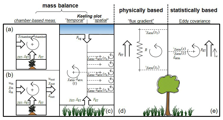
Figure 3Summary of the different approaches (mass balance, physically, and statistically based) methods for determination of δET with the relevant variables and fluxes for each case.
There is naturally a strong link between the temporal resolution in estimates and the temporal extent of the time series (Fig. 2b). The vast majority of the studies (85 %) provided values at hourly to subweekly resolutions over periods of time not exceeding a few months. This is partly a sign of the limitation of the isotopic methodology, which was mentioned in the Introduction, i.e. the labour-intensive and time-consuming destructive sampling of soil and plant material and the subsequent water extraction step. In two studies only (Hsieh et al., 1998; Ferretti et al., 2003), authors could calculate at weekly to monthly resolutions over several years. For doing this, they made a series of abovementioned simplifying hypotheses, which allowed them, amongst other things, not to rely on sampling of plant material, thereby significantly saving extraction and analysis time. The authors of the present work note that, on the other hand, the question of spatial variability or representativeness of the estimates is rarely addressed in the literature (but see Sect. 3.1 for the issue of spatial representativeness of δET).
In this section, the methods used for determination of the three terms in the partitioning equation (Eq. 1), i.e. δET, δE, and δE, for final computation of will be covered (Sect. 3.1.1, 3.2.1, and 3.3.1, respectively), with special emphasis on challenges and new technical and methodological developments (Sect. 3.1.2, 3.2.2, and 3.3.2, respectively). Three main approaches emerge from the analysis (Fig. 3): δET, δE, and δE can be either determined by
- i.
solving the mass balances for the different water vapour isotopologues,
- ii.
using physical models based on macroscopic analogies of Ohm's law, or
- iii.
using a statistical framework.
Note that it is not the present work's intention to give a thorough review of the physically based and isotope-enabled soil–vegetation–atmosphere numerical models used by Haverd et al. (2011), Sutanto et al. (2012), and Rothfuss et al. (2012) for simulation of . For this, the readers may refer also to Haverd and Cuntz (2010) and Braud et al. (2005). Likewise, the authors choose not to describe one particular ensemble of methods in detail (used in seven different studies; see Table 2 and referred to as “water balance” in Fig. 2.) based on solving a water mass balance equation and not relying on the sampling or monitoring of plant and soil water and atmospheric water vapour.
3.1 Isotopic composition of evapotranspiration
3.1.1 Methods
The prevalent method (43 % of the reviewed studies, Fig. 2h) for determining the isotopic composition of ET is based on solving a mass balance equation (Fig. 3a–c). It was named after Charles D. Keeling who originally used it to quantify the CO2 carbon isotopic composition in the atmosphere as a linear function of the reciprocal of the CO2 concentration (Keeling, 1958). The so-called Keeling plot technique simply considers that the water vapour measured in some ecosystem atmosphere (of concentration Catm and dimension of M L−3), e.g. within or above the canopy, originates from two sources, namely (i) the background water vapour (of concentration Cbg, M L−3), transported advectively and defined as not being influenced by ET flux, and (ii) evapotranspiration ET (of concentration CET, M L−3):
Practically, laser-based spectrometers measure the water vapour volume mixing ratio, χ (–), the ratio of water vapour pressure and total (dry) atmospheric pressure:
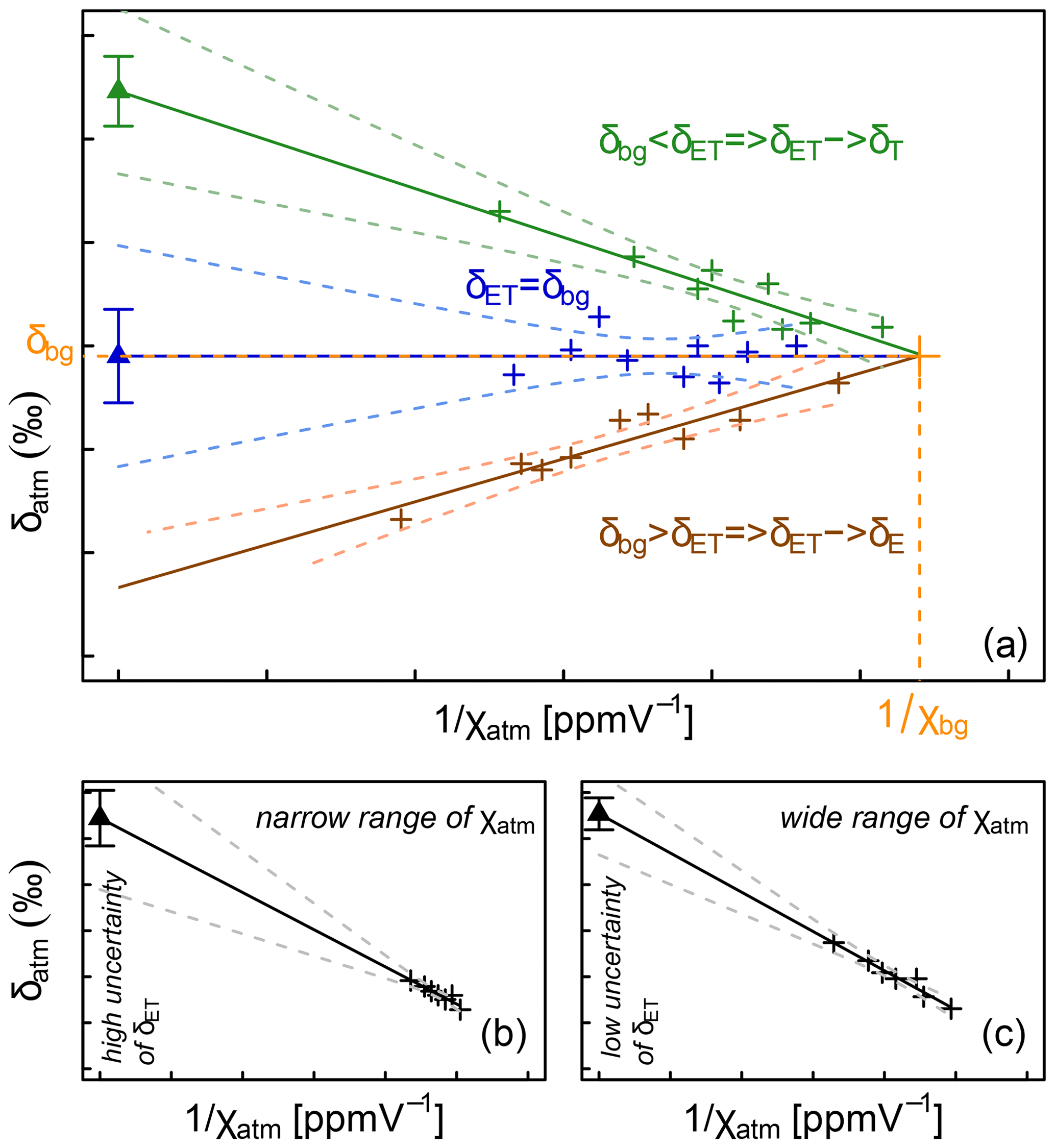
Figure 4Illustration of the Keeling (1958) plot technique for determination of the isotopic composition of the surface flux, here evapotranspiration (δET). Subscript “bg” refers to the atmospheric background air, i.e. the air, which is not influenced by the surface ET flux. (a) Cases with different slopes of the regression line and implications for the nature of the surface flux: ET tends either toward transpiration (T) or evaporation (E). Illustration of the importance of the (narrow or wide) spread in values of the water vapour mixing ratio (χatm, ppmV) for the uncertainty of the δET estimate (b, c).
A similar equation can be written for stable isotopes:
with δatm and δbg being the isotopic compositions of the ambient air and background air, respectively. Combining Eqs. (3) and (4) and rearranging for δatm leads to the following expression (Eq. 5; see Fig. 3 for an illustration):
To the conditions that
- i.
both χ and δ values of the background water vapour and ET remain constant during the measurement period and
- ii.
there is no loss of water vapour from the atmosphere (e.g. during dewfall),
it is possible to determine δET as the y intercept of the regression line of the relationship between δatm and . In this framework the sign of the linear regression slope s = is therefore constrained by the difference (δbg − δET); s is generally negative, apart from some bare-soil situations (Yakir and Sternberg, 2000) (Fig. 4a). Note that it is also possible to derive δET by inverting the expression for s, although, to our knowledge, such a possibility has not yet been tested in the literature, certainly because the determination of Cbg and δbg is not straightforward in the field.
One important prerequisite for the applicability of the Keeling plot is a significant span in χatm values over the course of the measurements (Fig. 4b and c). High χatm values are especially needed to reduce the statistical uncertainty of δET (Good et al., 2012). In the case of a single observation height (Wei et al., 2018, 2015; Good et al., 2014), the time factor is critical. χatm variations should not be obtained at the expense of the validity of the aforementioned core assumption (i), i.e. steady values of δET and background χ and δ. Another option beside the one just described, which we could refer to as the “temporal Keeling plot”, is to drastically increase the span of χatm values by collecting data at different observation heights during a short period of time (∼ 1 h), which could be referred to as the “spatial Keeling plot”. From our literature compilation, the spatial Keeling plot is preferred over the temporal one (i.e. 32 vs. 7 studies).
Another technique (18 % of the reviewed studies, Fig. 2h) for determining δET requires the manipulation of transparent chamber systems to enclose and tightly seal the soil and vegetation (e.g. Yepez et al., 2005; Piayda et al., 2017). Two different applications exist, both based on the mass balance approach. In the first one (referred to as “Chamber (InOut)” in Table A1 and Fig. 2h), the chamber is flushed with ambient air, and δET is deduced from the difference in the water vapour mixing ratio and isotopic composition measured alternatingly at the inlet (subscript “in”) and outlet (subscript “out”) of the chamber (e.g. Wang et al., 2013; Dubbert et al., 2013):
Equation (6) is strictly valid only for conservative flow conditions. In other studies (e.g. Dubbert et al., 2014b), the change in flow rate (u L3 T−1) between the in- and outlet due to the addition of water vapour originating from the soil and/or the plant is taken into account as follows:
By conservation of dry airflow, i.e. (Simonin et al., 2013), Eq. (6') becomes
The second term on the right-hand side of Eq. (7) therefore accounts for the increase of flow rate due to ET in the chamber. An alternative consists of flushing the chamber with dry air instead of ambient air so that the isotopic composition of the outlet water vapour directly reflects that of ET. In the second application (named “Chamber (Keeling plot)” in Fig. 2h), the chamber is flushed in a closed loop with ambient air, and δET is obtained by linear regression of the isotopic composition of the chamber air vs. the inverse of the water vapour mixing ratio using the Keeling (1958) plot technique.
In 10 % of the referenced studies (Wen et al., 2016; Wei et al., 2018; Zhou et al., 2018), authors determined δET values by analogy to Ohm's law. The so-called “flux gradient method” (Lee et al., 2007) is based on the premise that the ET flux density rate (FET, , expressed typically in ) is proportional to (L−1, typically in m−1), the gradient of water vapour mixing ratio between two observation heights (with zatm standing for height):
The water vapour transport is determined by the overall conductance of the air boundary layer expressed here as with ρatm (M L−3) and Matm (M L−3, units of kg mol−1) being the volumetric mass and molecular weight of dry air and K (L2 T−1) being the eddy diffusivity of water vapour. The isotopic ratio of ET (RET, –), which can be defined as the ratio of the flux density rates of the rare (superscript i) and abundant (superscript j) isotopologues (iFET and jFET, respectively), can be therefore expressed as
assuming that differences in K among water stable isotopologues are not significant, i.e. (Yakir and Wang, 1996; Griffis et al., 2005). iχatm and jχatm are the water vapour mixing ratio of rare and abundant isotopologues, respectively. Equation (9) can be further rearranged as
where RET is the slope and C (–) is the y intercept of the linear relationship between iχatm and jχatm. Equation (10) becomes in δ notation
by dividing its left and right terms by jχatmRstd with Rstd, the isotopic ratio of the internationally accepted water standard, namely the Vienna Standard Mean Ocean Water (V-SMOW) (Gonfiantini, 1978). We note that, by assuming jχatm≈χatm, the flux gradient and Keeling plot techniques are mathematically identical if , with s being the Keeling plot slope.
Griffis et al. (2010) and Good et al. (2012) used a combination of the EC technique and infrared tunable-diode-laser (TDL) water isotope spectroscopy to derive δET values from simultaneous changes in wind velocity (ω, L T−1) and iχatm. In this statistical framework and by
- i.
considering that air density and storage fluctuations are negligible during the measurement period (typically 30 min) and
- ii.
changing the coordinate system so that the vertical wind velocity mean value () equals zero,
FET is expressed as
The term is the average (overbar symbol) product of the differences between instantaneous and mean values (indicated by the prime symbols) of wind velocity and water vapour mixing ratio, in other words the covariance between the ω and χatm monitored variables. Similar to Eq. (11), we obtain after converting into δ notation the expression for the isotopic composition of ET:
An alternative to Eq. (13) consists of considering the high-frequency variations of δatm rather than those of the individual mixing ratios iχatm and jχatm. For this the isoflux (Lee et al., 2009), defined as (), is introduced:
3.1.2 Progress and challenges
In a review of isotope techniques for determination of the concomitant flux and isotopic composition of evapotranspiration, Griffis (2013) summarized the inherent limitations of the Keeling plot technique from the literature. The general assumption that atmospheric water vapour and its isotopic composition result from the turbulent mixing of only two sources was reported to be often violated. Reasons for this may be strong vertical gradients of the water vapour mixing ratio and isotopic composition or strong differences between δE and δE leading to the emergence of diffusion and air entrainment processes (Lee et al., 2006, 2012). The spatial Keeling plot suffers particularly from the fact that the different heights at which δatm is measured are representative for differently footprints areas of the studied ecosystem. While this may not be a problem for a homogeneous cropland, the reliability of the Keeling plot should be generally questioned for mixed vegetation (such as represented in Fig. 1) with strong lateral variabilities not only in δatm and χatm but also in soil water isotopic composition. In addition, the application of the spatial Keeling plot should not be conditioned based on a wide span of χatm values only but naturally on the quality of its linear fit. Griffis (2013) argued as well that the flux gradient approach suffers from a narrow range of application; e.g. it may not be suitable in certain cases, such as below forest canopies or above tall vegetation.
Regardless of these limitations or complications, Good et al. (2012) and Hu et al. (2020) provided comprehensive comparisons of the various techniques (Keeling plot, flux gradient, and EC) for determination of δET. In addition to the temporal and spatial variations of the Keeling plot, Good et al. (2012) tested a third option where, instead of instantaneous measurements of δatm and χatm collected during 30 min, the mean values of δatm and χatm are calculated at each observation height (n=4) and used for regression. After a detailed uncertainty analysis, they concluded that the use of mean values instead of individual data points increased the uncertainty associated with δET, regardless of the kind (temporal vs. spatial) of Keeling plot. In addition, the techniques of the temporal and spatial Keeling plot yielded significantly different values of δET for the same time interval. The authors could not conclude which value was the most representative. In addition, they found a good agreement between the Keeling plot technique, applied at different heights, and the flux gradient method due to the aforementioned mathematical similarities. Hu et al. (2020) compared at one irrigated maize crop δET values determined with either the Keeling plot or the flux gradient approaches. They tested different regression models with the Keeling plot method, i.e. ordinary least-squares regression, geometric-mean regression, and York's solution (for details see Pataki et al., 2003; Wehr and Saleska, 2017). These models differ in the way errors made on and δatm (see Eq. 5) relate to each other and whether they may be considered constant over their measurement ranges. As such, they yield differences in δET estimates. Hu et al. (2020) could illustrate the necessity of choosing an appropriate regression model that reflects the dependency of spectrometer-specific errors on the water vapour mixing ratio. Yepez et al. (2005) and Wang et al. (2013) combined the Keeling plot technique with their closed chamber systems. During the course of measurement (e.g. 6 min in the study of Yepez et al., 2005) and for the Keeling plot approach to be valid, the increase of the chamber water vapour mixing ratio (10–15 mmol mol−1 in Yepez et al., 2005) should not induce changes in both ET flow rate and isotopic composition. The fulfilment of this requirement of the Keeling plot technique is verified in a first approach by the very existence of a linear relationship between chamber air and δ values. However, it could be argued that the linear form of the regression equation should survive a linear change in either or δatm. Another issue related to the use of chamber systems is the occurrence of water vapour condensation on the inside of the chamber or within the tubing system, e.g. following changes of incoming solar radiation during measurement. This may result in eventual isotopic fractionation leading to unreliable (i.e. unstable and underestimated) observations of chamber air δ values. To avoid such problems, the volume of the chamber is critical (i.e. the bigger it is, the less sensitive it is to abrupt changes of outside conditions), and active ventilation is mandatory. Ventilation not only prevents from condensation problems and pressure anomalies (Longdoz et al., 2000) but also guarantees the prevalence of turbulent mixing conditions in the chamber. The latter may not be ensured by a high turnover rate alone, i.e. the ratio of chamber volume and flow rate of flushed air. It is an important prerequisite of the application of both techniques based on the Keeling plot and alternating measurements of the water vapour mixing ratio and isotopic composition of inlet and outlet air (Eq. 7). Measurements with dynamically purged chambers, which are combined with the latter type of mass balance applications, may reduce the problem of condensation inside the chamber. A possibility is to flush the chamber with dry air so that the increase in water vapour mixing ratio and (positive or negative) change of the isotopic composition measured at the outlet relative to the inlet directly reflect the volume and isotopic composition of the moisture added by ET. Stable measurements over a certain time period, depending on both chamber volume and inflow rate, would indicate ISS, and δET may be directly measured without any further calculations (e.g. Wang et al., 2010). However, dry air can stress the enclosed plants by artificially increasing the chamber air vapour pressure deficit, which ultimately can result in NSS conditions. In this case, a steady increase of chamber air χ should not be observed during the course of the measurement, as it would be a sign of a significant difference of micrometeorological conditions (temperature, vapour pressure deficit, and wind speed values) between ambient and chamber air.
As stated above, both the techniques of the temporal Keeling plot and the flux gradient suffer from the need of a high spatial gradient in the water vapour mixing ratio and isotopic composition between the soil or canopy surface and the free atmosphere to obtain precise values of δET. One alternative to sampling water vapour in atmospheric profiles at fixed heights is to use a small (about a few metres high) field lift system, the modus operandi of which is based on the principles established by Mayer et al. (2009) and Noone et al. (2013), for a continuous monitoring of atmospheric height profiles of the water vapour isotopic composition. To the authors' knowledge, only one study on an evergreen forest made use of the principle in the context of ET partitioning (Berkelhammer et al., 2016). Ney and Graf (2018) designed a portable lift system for measuring the atmospheric water vapour and CO2 mixing ratios in the field for various crops at a half-hourly temporal resolution. Their system should allow for measuring highly vertically resolved water vapour isotopic profiles. For this, however, high-throughput and high-frequency isotopic analysers are needed to provide reliable information on ecosystem fluxes. Commercially available cavity ring-down laser spectrometers operate at low flow rate (φ) and frequency (f) (e.g. 35 mL min−1 and f≈ 1 Hz for the L2120-i, L2130-i, and L2140-i by Picarro, Inc., Santa Clara, CA, USA) and are, thus, not suitable for such measurements. Other isotope analysers, such as the quantum-cascade-laser (QCL) trace gas monitor (Aerodyne, Inc., Billerica, MA, USA; φ≤ 250 L min−1 and f = 10 Hz) have the potential to fulfil the abovementioned requirements.
Compared to the Keeling plot and flux gradient approaches, the eddy covariance technique derives from micrometeorological theory (first principles). Where applicable, this makes it a solid alternative less subjected to assumptions. However, as a result of its high data acquisition rate and associated noise, the EC technique provides δET estimates with higher uncertainty, largely determined by random measurement errors (Hollinger and Richardson, 2005; Loescher et al., 2006; Rannik et al., 2016). Good et al. (2012) determined this uncertainty to be proportional to the inverse of the correlation coefficient between ω and χatm, i.e. the covariance of ω and χatm divided by the product of their measurement errors.
One important feature of the EC isotope technique resides in its ability to provide δET estimates at the field scale and therefore demarks itself from the abovementioned approaches. Griffis et al. (2010) and Griffis et al. (2011) demonstrated the reliability of δET data obtained with the eddy covariance technique from the agreement between measurements of the water vapour mixing ratio and ET flux of their traditional infrared analyser (LI-7500, LI-COR, Inc., Lincoln, NE, USA) and a fast-response and high-frequency water isotope spectrometer, i.e. the lead–salt tunable-diode-laser spectrometer TGA200A (Campbell Scientific, Inc., Logan, UT, USA; φ = 1.7 L min−1 at f = 10 Hz). However, to our knowledge, the production of this instrument has been discontinued. Recently, Braden-Behrens et al. (2019, 2020) showed that EC measurements could be performed using a high-flow (φ≈ 4.2 L min−1) laser spectrometer clocked at 2 Hz only (2 Hz-HF-WVIA, Los Gatos Research Inc., San Jose, CA, USA). They underlined the importance of heating the sampling tubing at the point of intake in order to avoid problems of condensation and high-frequency dampening as shown by spectra and cospectra.
3.2 Isotopic composition of evaporation
3.2.1 Methods
Two options are found in the literature (Fig. 2i) for determining the isotopic composition of the E flux, δE:
- i.
by solving one of either mass balance equations (Eqs. 7 or 11; see Sect. 3.1) in combination with dynamically purged closed bare-soil chambers (15 % of the reviewed studies, e.g. Dubbert et al., 2013, 2014b) or
- ii.
by solving the so-called “Craig and Gordon equation” (Eq. 18 below), which is derived from the atmospheric part of a transport model of water stable isotopologues, based on an analogy to Ohm's law (Craig and Gordon, 1965) (69 % of the studies).
The two approaches differ in numerous aspects: while the first is non-destructive and requires online and continuous measurements of a few variables (i.e. water vapour mixing ratio and isotopic composition of the chamber inlet and outlet air), the second relies – with the exception of the study of Quade et al. (2019) – on destructive sampling of the soil and offline analysis of the extracted water. The Craig and Gordon equation demarks itself from Eqs. (7) and (11) also due to its complex parametrization. Craig and Gordon (1965) classically interpreted the temporal changes in δE of a free water body with the help of a linear-resistance model. We will shortly present the widely used model variation for water bound to the soil media (for an in-depth review, the reader is kindly referred to Horita et al., 2008). The only significant difference to the original model is the evaporating front vertical coordinate (zEF), which may not correspond to that of the soil surface depending on the evaporation stage (Or et al., 2013; Merz et al., 2018). The isotopic ratio of evaporation, RE, is expressed as the ratio of iFE and jFE, i.e. the water vapour flux density rates () in rare and abundant isotopologues, respectively, originating from the EF:
We note that Eq. (15) is analogous to Eq. (9) (Lee et al., 2007; see Sect. 3.1), with the exception that the bulk resistances to vapour transport of the rare and abundant isotopologues (ir and jr, respectively, T L−1) are not assumed equal. It follows from the fact that ir and jr relate to the air layer delimited between zEF and zatm (and not between the two observation heights in Eq. 9), where not only purely turbulent transport or eddy diffusivity but also molecular diffusion and laminar flow are relevant. Furthermore, Craig and Gordon (1965) conceptualized the existence of a water-vapour-saturated (superscript “sat”) air layer at the EF where isotopic thermodynamic equilibrium prevails:
where Rsat and REF are the isotopic ratios of the saturated air layer and of the soil liquid water at the EF, respectively. αeq (–) is the isotopic equilibrium fractionation factor, first empirically determined by Horita and Wesolowski (1994). αeq depends on the soil temperature at the EF (TEF, K):
with constants , , and C = 0.052612 for 2H and , , and C = −0.0020667 for 18O. Craig and Gordon (1965) identified the ratio of bulk resistances as the isotopic kinetic fractionation factor (αK, –). Finally, by
- i.
considering that iχatm(zatm)=jχatm(zatm)Ratm,
- ii.
dividing the right-hand term numerator and denominator of Eq. (15) by , and
- iii.
converting RE into δE, we obtain:
where hatm (–) is the relative humidity of the ambient atmosphere measured at vertical coordinate zatm and defined as the ratio . The possible difference in temperature measured at zatm and zEF should be accounted for by normalizing hatm to the saturated vapour pressure (, usually expressed in Pa) at the temperature of the EF (Rothfuss et al., 2010; Quade et al., 2019).
Craig and Gordon (1965) argued that the kinetic fractionation factor was inversely proportional to the ratio of the molecular diffusivities of (jD) and of either 1H2H16O or (iD):

Figure 5Effect of the water status of the soil, i.e. the positioning of the evaporating front (EF, dashed line), on the value of the kinetic fractionation factor (αK). Panels (a–c) refer to the situation of a saturated soil (subscript “wet”) where the EF is located at the soil surface; panels (d–f) refer to a dry soil with the EF below the soil surface. The corresponding soil water total (tot; solid line), liquid (liq; dotted line), and vapour (vap; dash-dotted line) isotopic flux profiles (Ei, M L−3) (a, f); soil liquid isotopic composition profiles (b, e) are reported as well. Adapted from Braud et al. (2005).
Merlivat (1978) and later Luz et al. (2009) quantified the diffusivity ratios at 1.0251 and 1.0285 for 1H2H16O or isotopologues, respectively. Dongmann et al. (1974) (but see also Brutsaert, 1975) extended Eq. (19) to different aerodynamic regimes in the air boundary layer delimited by zEF and zatm:
where n (–) is an unitless factor ranging from 0.5 (corresponding to fully turbulent conditions) to 1 (fully diffusive), with a value of representative of laminar-flow conditions. Mathieu and Bariac (1996) proposed to define n in the case of evaporation from soil as a linear function of soil volumetric water content observed in the surface layer (θsurf; L3 L−3, typically in cm3 cm−3). n would range between 0.5 when θsurf reaches θsat, the water content value at saturation, and 1 for θsurf=θres, the value of residual water content (see Fig. 5).
In Mathieu and Bariac's conceptual framework the establishment of a dry soil surface layer results in added isotopic resistance by increasing the relative importance of gaseous molecular diffusion (i.e. in the tortuous soil pore network) in the overall transport of water vapour from the EF towards the well-mixed atmosphere. In the case of a fully water-saturated layer in contact with the free atmosphere, the opposite happens: water vapour leaving the rough surface is preferentially transported in a turbulent manner, leading to smaller n values.
3.2.2 Progress and challenges
To calculate δE with the Craig and Gordon equation requires simultaneous observations of hatm, TEF, δatm, and δEF. The first two variables are typically monitored with e.g. capacitive sensing. As for δatm, its value is determined from online or offline isotopic analysis after sampling of the atmospheric water vapour (see Sect. 3.1).
The variable most challenging to estimate is δEF (Fig. 5b and e). It greatly depends on how soil is sampled at the EF. However, there is no consensus on how this should be done in the literature (see the column on isotopic measurements in Table A1). Some studies do not precisely report the soil depth, which is considered to be the EF (e.g. Wang and Yakir, 2000; Yepez et al., 2003; Williams et al., 2004). In other studies (Yepez et al., 2005; Zhang et al., 2011; Dubbert et al., 2013) soil profiles are partially or entirely sampled at higher vertical (centimetre) resolution. Pioneer works on isotopic transport in saturated or non-saturated isothermal soils under steady-state evaporation (Zimmermann et al., 1967; Allison, 1982; Barnes and Allison, 1983) showed that the EF, i.e. the theoretical and continuous boundary between the soil “regions” dominated by either liquid or vapour flow (Fig. 5a and f), is associated with the highest isotopic composition () value of the liquid soil water (Fig. 5d–f). Later this family of models was extended to unsaturated soil water conditions, non-isothermal conditions, and time-variable evaporation flux (e.g. Barnes and Allison, 1988; Barnes and Walker, 1989). More recently, Braud et al. (2005) and Haverd and Cuntz (2010) implemented isotopic transport in both liquid and vapour phases of the soil, with a coupling to temperature dynamics, in numerically solved SVAT models (SiSPAT-Isotope and Soil–Litter–Iso). All the abovementioned studies underline the localized character of the EF and the strong isotopic gradient in liquid water at its location. The determination of the EF location may be problematic, especially in the case of a receding EF (zEF≠zsurf, Fig. 5d), which is generally the case in arid regions between rare precipitation events. Thus, sampling soil roughly from the surface does not allow for a precise determination of δEF and may lead to errors in δE estimates. Rothfuss et al. (2010) could demonstrate for a well-watered soil (i.e. with zEF=zsurf, Fig. 5b) that sampling of only a few centimetres of soil at the surface and using the corresponding δsurf in Eq. (18) could lead to a significant underestimation of δE. This would lead in turn to an overestimation of , since negative changes in δE translate into positive changes in , i.e. (when δET < δE, which is generally the case). The spatial (vertical) resolution of the soil sampling should therefore be as high as possible to be able to identify zEF precisely. For their specific case, Brunel et al. (1997) estimated also that the determination of the δEF value was the greatest source of uncertainty of .
After sampling in the field, water is recovered from the soil in the laboratory using one of six extraction methods: cryogenic vacuum extraction (Araguás-Araguás et al., 1995; West et al., 2006), azeotropic distillation (Revesz and Woods, 1990), direct vapour equilibration (Wassenaar et al., 2008), high-pressure mechanical squeezing (Kelln et al., 2001), centrifugation (Mubarak and Olsen, 1976), or microwave extraction (Munksgaard et al., 2014). Other methods include the use of soil liquid water samplers (Wenninger et al., 2010; Sutanto et al., 2012). Finally, δEF is measured by isotope ratio mass spectrometry (IRMS) or isotope ratio infrared spectrometry (IRIS). Note that an alternative consists of letting soil water directly equilibrate with CO2 without the need for water extraction (one study is Ferretti et al., 2003, which follows the method of Scrimgeour, 1995). In this framework, pure CO2 is injected in the exetainer containing the soil sample following evacuation. After a 3 d long water–CO2 equilibration period, the δ18O value of CO2 is measured by isotope mass spectrometry and used to infer that of water at equilibrium. Orlowski et al. (2016a, b) provided evidence from laboratory benchmarks of the different techniques that the isotopic composition of the recovered water could be sensitive to the extraction approach and extraction time as well as to the soil type and values of water and organic content. The same authors also observed that IRMS and IRIS techniques yielded different results in general and especially for clay loam soil water, which they related to interferences in the absorption spectrum during analysis with the latter technique. In addition, Orlowski et al. (2018) concluded from a worldwide inter-comparison of cryogenic-vacuum-extraction facilities that the general consensus in the isotopic ecohydrology community, stating that cryogenic vacuum extraction is the standard water recovery technique, should be questioned. Orlowski et al. (2016a, b, 2018) highlighted the limitations of the most popular extraction approach, i.e. based on the combination of destructive sampling and vacuum extraction (69 % of the reviewed studies), which calls for the development of other techniques for a precise quantification of δEF.
In the last few years Rothfuss et al. (2013), Volkmann and Weiler (2014), and Gaj et al. (2016) successfully validated and tested alternatives to destructive sampling and offline isotopic analysis approaches. They developed systems based on the combination of gas-permeable membranes (e.g. rigid hydrophobic microporous polypropylene, Membrana GmbH, Germany, or polyethylene, Porex Technologies, Aachen, Germany) with laser-based spectrometry for the non-destructive collection of the soil atmosphere and the online monitoring of its water vapour isotopic composition (). For this, the soil atmosphere is either
- i.
flushed with a carrier gas (dry synthetic air, i.e. 20.5 % in N2, or 100 % N2) at low flow rate in the range of 50–100 mL min−1 (Rothfuss et al., 2013; Volkmann and Weiler, 2014; Gaj et al., 2016) or
- ii.
extracted with a vacuum pump (Volkmann and Weiler, 2014).
Both modi operandi allow for long-term and repeated measurements across the soil profile provided that condensation is avoided in the sampling line. For this, the collected air, which is (quasi-)saturated with water vapour, is diluted with the carrier gas and the sampling lines are heated, if necessary (Quade et al., 2019; Kühnhammer et al., 2019). Rothfuss et al. (2013) observed near-isotopic-equilibrium conditions between liquid and vapour in the soil pore space and provided temperature calibration equations yielding results analogous to those of Horita and Wesolowski (1994) for converting into values. They further show that isotopic equilibrium conditions still prevailed at low soil volumetric water content, possibly also for soil water vapour relative humidity values lower than 1. Their method was successfully applied to laboratory experiments with sand (Gangi et al., 2015; Rothfuss et al., 2015) and silt loam (Quade et al., 2018). Oerter et al. (2017) compared values estimated with the monitoring method of Rothfuss et al. (2013) on the one hand and the direct equilibrium and vacuum extraction methods on the other hand. They found a good correlation between the two approaches (root mean square error – RMSE – equal to 0.6 ‰ for δ18O and within 1.7 ‰–3.1 ‰ for δ2H). Volkmann and Weiler (2014) tested their own design of a water vapour probe under field conditions and could show that it produced values in agreement with those following destructive sampling and isotopic analysis with the direct equilibration method (Garvelmann et al., 2012). The inter-method (destructive vs. non-destructive) RMSE values were comparable to the intra-method variability of soil water δ values. The latter variability could not be disentangled into systematic methodological error and natural (lateral) heterogeneity in soil water isotopic composition. Kübert et al. (2020) conducted a comparison study of the method of Rothfuss et al. (2013) with cryogenic vacuum extraction and centrifugation during an irrigation pulse-labelling experiment in a semi-natural temperate grassland. They highlighted that the non-destructive method could capture temporal dynamics of the isotopic composition, while destructive sampling included both the temporal change and spatial heterogeneity.
To date there are two ET partitioning studies, in which δE was determined from non-destructive isotopic analysis using soil-liquid-water–water-vapour equilibration. Quade et al. (2019) applied the method of Rothfuss et al. (2013) in a sugar beet field in a temperate climate (Germany), while Gaj et al. (2016) used commercially available soil gas probes (BGL-30, METER Group, Munich, Germany), following the same modus operandi as Volkmann and Weiler (2014), during a field study in central Namibia under semi-arid conditions. Such applications are promising for the specific purpose of partitioning ET, as they provide insights into subdaily dynamics of δE from the online assessment of the positioning and isotopic composition of water at the EF. However, one noticeable disadvantage is the need for deploying a laser spectrometer at the experimental site. A possible way around has been recently proposed by Havranek et al. (2020) as a compromise: water vapour samples are collected and stored automatically in flasks from the soil profile in the field following the approach of Rothfuss et al. (2013) and transported back to the laboratory where the isotopic analyses are performed.
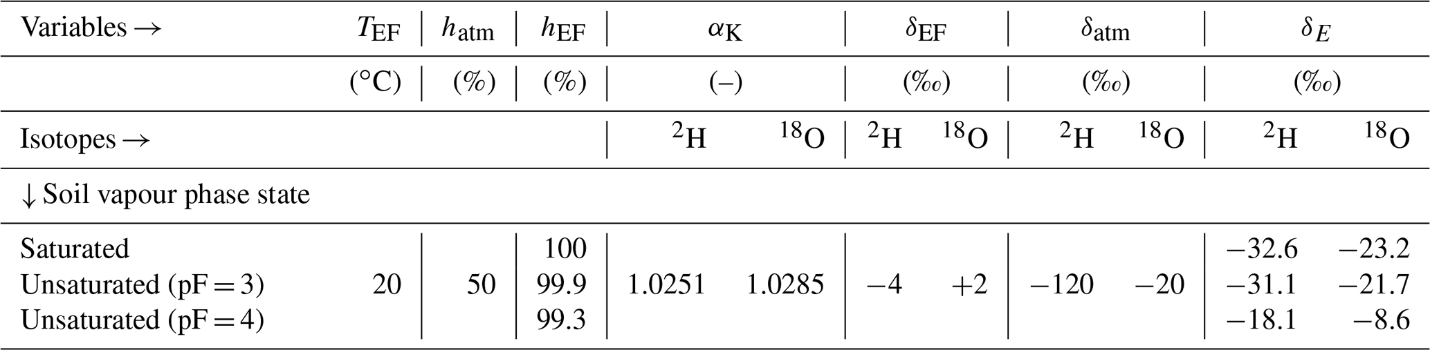
Table 1Effect of the consideration of non-saturated soil water vapour phase on the estimation of the isotopic composition of evaporation (δE) using the model of Craig and Gordon (1965). Conditions of the transport of pure diffusive water vapour (n=1) prevail, leading to values of the kinetic fractionation factor (αK) of 1.0251 und 1.0285 for 2H and 18O. Values for TEF, hatm, δEF, and δatm are chosen exemplarily.
Another important factor that influences the precision of δE estimates is the choice of the value of the kinetic fractionation factor, αK. Only a handful of studies attempted to estimate or model αK for soil E. Braud et al. (2009) simulated αK values during long-term laboratory experiments with the SVAT model SiSPAT-Isotope. They found a decreasing trend in αK value from saturated to unsaturated soil conditions, which contradicts the model of Mathieu and Bariac (1996). Results similar to the study by Braud et al. (2009) were obtained by Rothfuss et al. (2015) during a long-term soil column laboratory experiment. Quade et al. (2018) tested two different methods for quantifying αK during a series of bare-soil evaporation experiments on monoliths (100 L soil volume) under semi-controlled conditions, i.e. the following:
- i.
The first method is the inversion of the Craig and Gordon equation (Eq. 18) in a single isotope-framework (i.e. based on either δ18O or δ2H values) with input variables hatm, TEF, δatm, δEF, and δE.
- ii.
The second method is the inversion of the Craig and Gordon equation in a dual-isotope framework. More specifically, αK is determined from the approximation of the slope (S, –) of the soil E line (SE = , –) in a [δ18O, δ2H] coordinate system following Gat (2000):
with t being the time stamp and Δε (–) being the so-called kinetic effect, defined as
with superscripts i and j standing for the least and most abundant isotopologues, respectively. Equation (21) is solved in an implicit manner; in other words, SE values simulated for time stamp t depend on δEF observation made at time stamp (t−1). The n value is then extracted from Eq. (21) from the confrontation of measured and simulated SE, and finally fed into Eq. (19') to retrieve αK values. Quade et al. (2018) showed that αK could not be considered a constant value solely depending on flow conditions as proposed by Dongmann et al. (1974) or determined from soil water content following Mathieu and Bariac (1996) (Eq. 20). The second approach yielded αK values in agreement with the literature (e.g. Merlivat, 1979). Quade et al. (2018) concluded that turbulent transport still played a significant role during the evaporation process, also under non-saturated conditions. These studies show that further sensitivity analyses of αK to environmental conditions are needed to provide realistic estimates of δE and ultimately of values. To our knowledge, there is no ET partitioning study in the field where αK was considered to dynamically change (other than via the model of Mathieu and Bariac, 1996) depending on the contribution of air turbulence to water vapour transport in the free and canopy atmosphere, e.g. from measurements of the wind profile within and above the canopy (Brutsaert, 1975).
Another source of uncertainty arises from a lack of precise knowledge of the state of water vapour saturation at the EF (Braud et al., 2005; Rothfuss et al., 2015). In the Craig and Gordon equation, the kinetic fractionation factor is weighed by the term (hEF − hatm), where hEF is generally assumed to be equal to 1, representative of saturated conditions at the EF. However, this assumption may not stand for dry soils considering the relationship between soil water matric potential ψEF (, typically expressed in hectopascals or centimetres of water height) and pore space relative humidity at the EF (hEF), as given by Kelvin's law:
Mw and ρw (M L−3) are the molar and volumetric masses of water, respectively, and Rgas () is the universal gas constant. Table 1 presents three different degrees of saturation of the soil vapour phase under isothermal conditions (TEF = 20 ∘C) and their corresponding hydrogen and oxygen isotopic composition values of the E flux (δ2HE and δ18OE). A decrease in hEF from 100 % to 99.9 %, corresponding to an increase in the absolute ψEF value from 0 to 1000 hPa (i.e. from saturation to pF = 3) leads, for example, to an increase of 1.5 ‰ in δ2HE and δ18OE. A decrease in hEF from 100 % to 99.3 % (increase from 0 to 10 000 hPa, i.e. pF = 4) would translate into an increase of 13 ‰ in δ2HE and δ18OE. Both δ2HE and δ18OE are affected in the same way by the change in value of the factor (see Eq. 18), i.e. approximatively 2.0 ‰ per 0.1 % relative humidity. This may have a noticeable effect on the computation of , especially for δ18O, for which the difference of δE − δE is usually smaller than for δ2H. Gas exchange chambers and other experimental setups with semi-controlled conditions (such as weighing lysimeters) provide means to test the validity and existence of the abovementioned hypotheses and complications (e.g. Dubbert et al., 2013; Groh et al., 2018).
3.3 Isotopic composition of transpiration
3.3.1 Methods
The determination of the isotopic composition of T, δE, in the reviewed literature is mainly dependent on the underlying hypothesis of the isotopic steady or non-steady state (NSS) of T. While 42 % of all reviewed studies assume isotopic steady state (ISS), in other words that δE is time-invariant, 58 % do not make such an assumption but assume a transient state, i.e. NSS (Fig. 2j). This has substantial implications for the materials and methods used for the determination of δE. In the ISS approach, δE is directly inferred from the isotopic value of the leaf water source (δxyl), i.e. the water in the xylem vessels supplying the leaf water reservoir. This assumption is based on the fact that at ISS the flux density rate of the least abundant (iFxyl) (respectively most abundant, jFxyl) isotopologue entering the leaf equals the flux density rate of the least abundant (iFT) (most abundant, jFT) isotopologue leaving it by transpiration:
Note that in this framework an instantaneous change in jFT, if compensated by a corresponding change in jFxyl, should maintain the relationship δxyl=δT (Eq. 24b). In reality, a change in jFT, due to variations in environmental factors (e.g. vapour pressure deficit of the free atmosphere and incoming solar radiation) implies a change in root water uptake depth profile, which in turn affects δxyl in the case of a heterogeneous distribution of the soil water isotopic composition (Rothfuss and Javaux, 2017). A new ISS is eventually reached, depending on the leaf water turnover time, i.e. the ratio of leaf water volume and transpiration rate (Dongmann et al., 1974; see below). To access xylem water, authors destructively sample stems (e.g. Wei et al., 2018; Quade et al., 2019), branches (e.g. Williams et al., 2004), or root water (Bijoor et al., 2011) and recover their water by e.g. cryogenic vacuum extraction.
The NSS approach for determining δE relies either on direct non-destructive monitoring (i.e. leaf chamber-based measurements, e.g. Wang et al., 2010) or on destructive sampling of plant material and subsequent extraction of water (e.g. Dubbert et al., 2013). In the former case, the modus operandi is the same as when operating ET and E chambers coupled to mass balance equations (see Sects. 3.1 and 3.2, respectively), except that one single leaf or several leaves are enclosed in the chamber (with a volume ranging from 150 to 190 cm3 in the literature), rather than the entire plant. It is then generally assumed that the leaf-scale δE estimate is also representative for the whole plant (e.g. Good et al., 2014). In the case of destructive sampling, δE is modelled on the basis of environmental factors (leaf temperature and free-atmosphere relative humidity) and isotopic variables. Two cases can be distinguished.
- i.
δE is determined from the value of the isotopic composition of the leaf bulk water, δL, with the Craig and Gordon equation adapted to plant T (Sun et al., 2014; Hu et al., 2014):
- ii.
The isotopic composition of leaf water may not be available, but that of its source, δxyl, is. The δE value is calculated after the relationship of Dongmann et al. (1974), which describes the temporal course of δL at a constant transpiration rate value (i.e. at permanent flow for T). The authors expressed the rate of change in δL as a function of the instantaneous difference between δxyl and δE at time t, by considering the leaf bulk water (delimited by volume per unit leaf area VL, L3 L−2) to be transpired into ambient air at permanent flow (i.e. at density rate jFT=jFxyl, as in Eq. 24a):
By combining Eqs. (18') and (25) and considering that δxyl is time-invariant, we obtain a first-order differential equation for δL, which yields after integration to
where the leaf water turnover time, τL, is defined as the ratio and , the isotopic composition of leaf bulk water when an isotopic steady state is reached. The latter term is expressed as
By (i) noting and , where εeq and εK (–) are the equilibrium and kinetic fractionations, respectively, and (ii) dropping terms with products εeq⋅εK, we obtain the following expression of the difference in isotopic composition between leaf and source waters at ISS:
We note that Eq. (27') is the inversion of the Craig and Gordon equation at ISS, i.e. when δT=δxyl. Finally, δE is computed with the NSS Craig and Gordon equation, i.e. Eq. (18'). Equation (26) states that, at a permanent state for transpiration, the degree of attainment of ISS conditions in the leaf is a function of time, leaf internal dynamics (τL), and (isotopic) aerodynamic boundary conditions. The formula of Dongmann et al. (1974) requires two additional parameters as compared to the more “straightforward” application of the Craig and Gordon equation, namely leaf transpiration (jFT) and volume (VL), both labour-intensive to obtain and associated with high uncertainties.
Both case scenarios (i) and (ii) make the assumption that leaf water is a well-mixed reservoir, in other words that only convective transport of the water isotopologues occurs, leading to δL=δLts, where δLts is the isotopic composition of water at the leaf transpiration sites. However, a number of studies reported strong isotopic variations within the leaf water pool (i.e. among different compartments such as leaf veins, cell walls, and symplastic water; see e.g. Yakir et al., 1989; Wang et al., 1998, 1994; Bariac et al., 1994), which can be related to hydraulic separation of water pools and diffusive transport from the transpiration sites towards the petiole of the leaf. Another explanation may be found in the heterogeneity in opening of the leaf stomata (Farquhar et al., 2007). More specifically, δLts should be significantly higher than the bulk leaf water isotopic composition value, δL, which leads to an underestimation of δE by the direct application of the Craig and Gordon equation. Walker et al. (1989), Walker and Brunel (1990), and Flanagan et al. (1991) considered in a first approach two distinct water pools in the leaf, one in isotopic equilibrium with water vapour in the stomatal cavity (of isotopic composition δLts_ISS) and one isotopically undistinguishable from xylem water (of isotopic composition δxyl) in respective proportions p and (1−p). In these three studies, an analogous expression to Eq. (27') is used where p is accounted for:
They suggested that there was a midday maximum for T density rate from the corresponding minimum value for p. Cernusak et al. (2002) and Farquhar and Cernusak (2005) proposed a similar equation to that of Dongmann et al. (1974) for the evaporative isotopic enrichment in leaves in NSS conditions but without considering the leaf water volume per unit area constant in time. Equation (25) becomes in their case
By replacing δxyl and δE in the right hand-term of Eq. (25') with the ISS and NSS Craig and Gordon equation forms, respectively, the authors give an expression relating the rate of change of δL with the difference between δLts_ISSand δLts:
where jχint and jr are the water vapour mixing ratio in the intercellular space and, as in Sect. 3.2, the resistance to vapour flow of the isotopologue in air, respectively. It is therefore possible, by fitting the time course of the bulk leaf water isotopic composition δL to deduce δLts, on the basis of which δE is finally determined using Eq. (18') (Yepez et al., 2005). αeq is, as in Sect. 3.2, calculated following the closed-form equations of e.g. Horita and Wesolowski (1994) (Eq. 17). As for αK, its expression is adapted to include the series of flow resistances of water vapour isotopologues inside the stomatal cavity or through the stomatal opening (irsto and jrsto, T L−1) and in the leaf boundary layer (irbdl and jrbdl, T L−1) (Jarvis, 1976; Stewart, 1988). Farquhar et al. (1989) (and see also Cernusak et al., 2005; Farquhar et al., 2007) considered that molecular diffusion drives the transport of the different water vapour isotopologues in the first case and that turbulence prevails in the second, leading to n exponent values of 1 and , respectively (Dongmann et al., 1974; Eq. 19'). In this framework, αK is decomposed as
Cuntz et al. (2007) proposed a general iterative solution of the Dongmann et al. (1974) formulation revisited by Cernusak et al. (2002) (Eq. 28) under various scenarios depending on considerations regarding leaf water reservoir isotopic homogeneity (δL=δLts or δL≠δLts) and volume ( or ). Dubbert et al. (2013) applied their solution in the case of an isotopically well-mixed leaf water pool transpiring at constant volume and expressed the incremental change in δL from time step t to t+dt as
where gs (L T−1) is the total stomatal conductance.
3.3.2 Progress and challenges
The isotopic composition of T may be derived under NSS conditions from plant chamber measurements following Eq. (7) (Sect. 3.1), either at the leaf level or at the branch level. While most studies developed and operated custom-made chambers, only a few (e.g. Wang et al., 2010) used commercially available leaf chambers (e.g. LI-6400, LI-COR, Nebraska, USA). Chamber measurements have several disadvantages as discussed in Sect. 3.1 but are essential for monitoring δE directly without relying on additional modelling steps using either δxyl or δL. The important two features of the chamber-based method are that it does not require the assumption of ISS and that it allows for repeated (i.e. non-destructive) measurements on the same leaf or ensemble of leaves during the course of the day. On the other hand, the determination of δxyl or δL, which is largely based on destructive sampling and water recovery with e.g. cryogenic vacuum extraction, is also associated with uncertainty (e.g. Orlowski et al., 2016a, b; Millar et al., 2018). The choice of an appropriate method for sampling xylem water is also crucial for a correct determination of δE. For example, herbaceous, grass, or crop species do not have suberized stems; thus destructive sampling would have to rely on leaf water sampling or sampling the plant culm belowground, which is highly destructive and may not be possible on plots of common size. Recently, Chen et al. (2020) documented during a series of laboratory controlled experiments that the apparent offset measured between the hydrogen isotopic composition in sap xylem and source water of different mangrove plant species was the result of artefacts during the vacuum extraction process rather than due to isotopic fractionation during water uptake. This could be a reason for hydrogen isotopic offsets reported elsewhere in the literature (e.g. Ellsworth and Williams, 2007; Barbeta et al., 2019). If applicable to other species, the results of Chen et al. (2020) would suggest caution in determining values based on the determination of δ2HT directly from δ2Hxyl at ISS (Eq. 24b) or considering NSS conditions using e.g. the Craig and Gordon (1965) equation (Eq. 18').
A novel type of non-destructive method, first published by Volkmann et al. (2016) and recently by Marshall et al. (2020), could enable monitoring δE of trees at an equivalent temporal resolution and even greater temporal coverage than with leaf- or plant-scale chamber systems. In the former study, several 10 mm outer diameter gas probes designed after Volkmann and Weiler (2014) (see Sect. 3.2) were inserted into pre-drilled holes in the trunk sapwood of two individuals of Acer campestre L. The probes were positioned at breast height in various azimuths. By assuming isotopic equilibrium between the water vapour sampled by the probe and flushed to the laser spectrometer and the xylem (liquid) water, the authors computed δxyl values from the temperature-dependent relationships given by e.g. Horita and Wesolowski (1994). For comparison, tree sapwood was destructively sampled, and its water isotopic composition was measured with IRMS after cryogenic vacuum extraction. A good agreement was found between online measurements and offline analysis of xylem water hydrogen isotopic composition. The inter-method bias regarding the determination of xylem water δ18O was thought to be due to spectral interferences during online analysis with the laser spectrometer. The experimental natural conditions did not allow the authors to conclude if differences in δxyl among the different gas probes reflected actual diurnal variations in root water uptake or preferential connection between xylem vessels and specific parts of the root system that were not affected by the labelling pulse. The authors underline the difficulty with their experimental design to precisely measure the temperature of equilibration in the gas probe (needed for converting sample water vapour to xylem water isotopic composition), due to the high lateral temperature gradient and its daily course. Marshall et al. (2020) tested a cruder way (which they entitled the Borehole Equilibration) to sample water vapour originating from xylem water of two pine tree species (Pinus sylvestris L. and Pinus pinea L.) under semi-controlled conditions. Contrary to Volkmann et al. (2016), (i) the authors did not use a gas probe but simply connected a hole drilled horizontally through the trunk to a laser spectrometer with gas sampling lines. Furthermore, (ii) the experiments were performed in hydroponic water solutions to enable a quasi-instantaneous change of the isotopic composition of the water source, thereby setting defined lower isotopic boundary conditions for further modelling efforts. To test the practicability of the method, the experimental results were confronted with a “Dongmann-like” NSS formulation of the isotopic composition of the water vapour stream, in which the geometry and its consequence on the diffusion from the borehole surface and on the establishment of laminar-flow transport were explicitly accounted for. With their model, the authors tested whether the sampled water vapour was in isotopic equilibrium with xylem water or was the product of evaporation from it. It was shown that the prevalence of a full isotopic equilibrium was a reasonable assumption and that the flow-through time (i.e. borehole volume divided by the flow rate) was 20 times greater than the time needed for diffusion of water vapour originating from the xylem vessels into the laminar-flow region in the middle of the borehole section. Both methods present a drastic advancement in isotopic analysis of xylem water and have great potential in the context of ET partitioning of forest ecosystems, on the pivotal condition that the steady-state assumption (δxyl=δT) applies during periods of measurements. The long-term applicability of the method, i.e. the ability of the investigated tree species to withstand the invasive and destructive installation of the probe, still needs to be proven at this point.
While the coupling between gas exchange chambers and laser spectrometers has the advantage of directly measuring δE, the aforementioned destructive sampling method and in situ monitoring technique quantify δL or δxyl, therefore potentially requiring a modelling step to obtain δE. A number of studies (e.g. Zhou et al., 2018; Wei et al., 2015; Aouade et al., 2016; Volkmann et al., 2016) assume ISS and hence treat δxyl as equal to δE. Although this assumption is probably justified for a daily integration, there is growing evidence that plants reach ISS only briefly in the course of a day, especially when environmental conditions change rapidly (Simonin et al., 2013; Dubbert et al., 2014b, 2017). Thus the analysis is greatly simplified by daily integration, if that is sufficient for the study objectives. Moreover, the leaf water turnover time, which can effectively be described by stomatal conductance (gs), vapour pressure deficit, and leaf water volume, is species-specific and ranges from several minutes to several hours (Song et al., 2015). As the leaf water turnover time describes the necessary time for leaf water to reach ISS (see exponent terms in Eqs. 26 and 30), ISS can either be observed for large parts of the day (e.g. in many herbaceous species) or not at all (e.g. in plant species strongly controlling their gs; see Dubbert et al., 2017, and Dubbert and Werner, 2019, for an overview). Therefore, the validity of assuming ISS for the purpose of ET partitioning will largely depend on the desired temporal scale: considering NSS is definitely necessary at subdiurnal to diurnal scales but unimportant at larger timescales. In case NSS is likely to occur, δE can be modelled using a “Dongmann version” of the Craig and Gordon equation, as shown in Sect. 3.3.1 (Dongmann et al., 1974). However, this complicates the partitioning approach considerably in comparison to direct chamber measurements of δE, as a large number of additional observations are necessary. In particular, gs and the canopy temperature are important input parameters. Therefore, the use of chamber measurements is highly recommended in any case.
The isotopic methodology for partitioning ET relies on a number of possible combinations of different techniques, which differ in numerous aspects. While some of them are based on destructive sampling and water recovery using one of the aforementioned methods (e.g. cryogenic vacuum extraction or direct liquid–vapour equilibration; see Sect. 3.2) and a posteriori analysis in the laboratory (e.g. for determination of δE using the Craig and Gordon equation), other methods are non-destructive, provide online measurements, and do not include a strong modelling component (e.g. determination of δE with plant chambers with one of two mass balance techniques). Destructive approaches require neither the handling of soil, plant, or soil and plant chambers nor the deployment of a laser spectrometer along with its conditioning system in the field. They should also allow for capturing the inherent spatial variability with repeated sampling (however, at the cost of long hours spent in sample preparation and water extraction). Non-destructive methods, such as chambers, may on the other hand provide environmental conditions for the enclosed plant that are not representative of ambient conditions.
Up to now only indirect methods, e.g. based on Scanlon and Kustas (2010), might have been able to provide continuous and subdaily estimates of . Some methods, such as the Keeling plot technique, can provide long-term continuous estimates of δET once a meteorological mast is installed in the field. It is, on the other hand, not advisable to enclose a plant in a chamber over longer time periods. Within the realm of destructive techniques, the user may assume ISS or test its existence when determining the isotopic composition of T. The techniques with which δET is estimated generally differ in terms of spatial significance as compared to those for determining δE and δE. Estimates of δET obtained either with the EC, Keeling plot, or flux gradient technique are thought to be representative at the field scale (e.g. as represented by the EC footprint). Note that this is also a problem encountered in (non-isotopic) instrumental approaches for partitioning ET, including EC, micro-lysimeters, and soil chambers (Kool et al., 2014). To account for these discrepancies in spatial representativeness, several micro-lysimeters and (if possible automated) chambers are deployed on site, e.g. within the framework of global networks (e.g. FLUXNET; Law et al., 2002). On the contrary, there has been no consensus to date on a common methodological ground for partitioning ET in the field on the basis of water stable isotopic measurements, depending on the type of land cover and use (agricultural, grassland, or forest ecosystems).
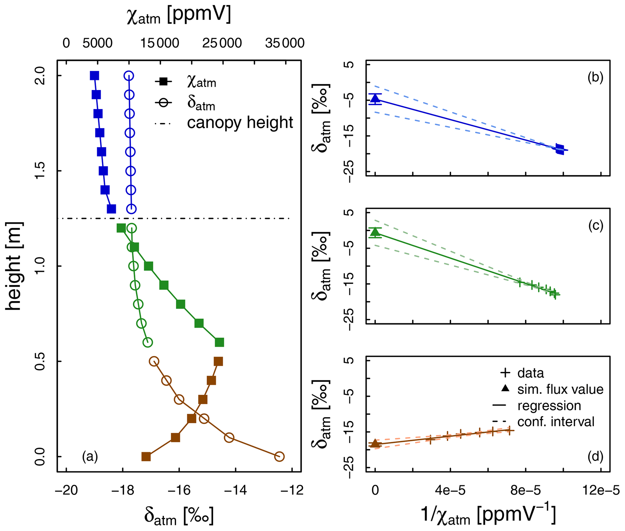
Figure 6One example of application of the Keeling (1958) plot technique to synthetic data that would be collected with a field-deployable lift at high vertical resolution (0.1 m) (for implications on measurement frequency, which also needs to be high (≥ 5 Hz), see Sects. 3.1 and 4 of Ney and Graf, 2018). The oxygen isotopic compositions of evapotranspiration, transpiration, and evaporation are estimated by the values of the y intercepts of the linear regressions between the isotopic composition of the atmospheric water vapour (δatm) and the inverse of the water vapour mixing ratio (χatm) in three non-overlapping regions, i.e. (i) the “free atmosphere” (indicated by the blue symbols), (ii) the region spreading from the canopy height to the height of the local maximum in δatm (green symbols), and (iii) the region delimited by the δatm local maximum height and the ground level (brown symbols). Also shown are the 95 % confidence interval envelopes of the linear regressions (dashed lines) as well as error bars (1 standard error) of the y intercepts.
It is the authors' belief that non-destructive and online methods integrated into automated sampling platforms and part of long-term (e.g. multi-year) water flux observatories should be preferred over destructive and discontinuous assessments of values. In this (ideal) framework, we propose the following:
- i.
The seminal effort in applying the EC technique by Griffis et al. (2010) should be continued to provide half-hourly and continuous ecosystem-scale δET estimates. The δET estimates obtained with the EC technique should be corroborated or confronted with the Keeling plot and the flux gradient approaches to identify possible scale-dependent disparities in surface isotopic signals as in Good et al. (2012).
- ii.
δE should be monitored by installing gas-permeable membranes or tubing (see Sect. 3.2) in the upper layers of the soil, depending on site-specific knowledge regarding the receding of the EF. While the gas probes of Volkmann and Weiler (2014) and Gaj et al. (2016) are better-suited for insertion at different locations in a soil profile, the membrane tubing used by Rothfuss et al. (2013), Oerter and Bowen (2019), and Kübert et al. (2020) allows for covering more ground surface by using a customized length of tubing. This should help to increase the representativeness of the δE value estimated from the soil water vapour isotopic composition and the use of the Craig and Gordon equation. When using the model of Craig and Gordon (1965), authors should systematically perform sensitivity analyses of
- a.
the depth of the EF and its water isotopic composition and
- b.
the value of the kinetic fractionation factor, αK.
These analyses will provide insights into the uncertainty of , in addition to the uncertainty originating from the solution of the two end-member equation (Eq. 1) (Rothfuss et al., 2010). This is, however, under-investigated according to our literature review. The αK value may be derived in a dual-isotope space using the formulation of Gat (2000) rather than based on unclear assumptions regarding the type of transport (molecular diffusion, laminar, or turbulent transport) controlling the flow of water stable isotopologues (see Sect. 3.2). As a side note (and without a proof of concept for this), the δE value may be directly determined in the case of a well-developed dry surface on the basis of non-destructive measurements of the soil water vapour isotopic composition () at two depths (z1 and z2) located between the EF and the soil surface. For this, the Craig and Gordon equation may be used without the need to locate the soil EF nor to assume liquid–vapour equilibrium:
- a.
- iii.
Several transparent flushed plant- or leaf-size chambers should be operated at the study site to characterize the in situ natural lateral heterogeneity of δE, due to differences in root water uptake, plant physiological state, and lateral heterogeneity in soil water isotopic composition profiles. This would be a prerequisite for any upscaling attempt of δE values. Developments should be made towards designing chambers able to mimic the dynamics of ambient air temperature, relative humidity, and wind turbulence to avoid biases in δE estimation. This could be done by cooling of the inlet air to avoid overheating of the air inside the chamber and with an adaptive active ventilation system. In situations where parts of the field are bare, e.g. between crop rows, soil chambers should be installed as well to evaluate differences in δE between areas covered or not covered with vegetation.
- iv.
The methods for monitoring of δxyl and its potential use in determining δE (that is by assuming ISS conditions) have been tested and validated with tree species exclusively. The same principle is yet to be minimized and applied to crops able to survive the installation and carry the instrumentation, such as a well-developed maize plant.
Lastly, the lift system principle, as operated by Noone et al. (2013), Mayer et al. (2009), and recently for agricultural crops Ney and Graf (2018) has the potential to provide half-hourly concomitant values of δET, δE, and δE in the field. The principle is illustrated in Fig. 6, further developing that of Yepez et al. (2003). The Keeling plot technique is applied to data collected at high vertical resolution (ultimately implying high-frequency data acquisition of the analyser, typically equal to or greater than 5 Hz; see Ney and Graf, 2018) in three distinct atmospheric regions, i.e. (i) the region spreading from the fully turbulent atmosphere to the canopy height, (ii) the region comprised between canopy height (here fixed at 1.25 m) and the local maximum in δatm, and (iii) the region delimited by the δatm local maximum and the ground level (Fig. 6a). The y intercepts of the three Keeling plots give the concomitant values of the isotopic compositions of ET (Fig. 6b), T (Fig. 5c), and E (Fig. 6d). In this synthetic experiment, which cannot be construed as a proof of concept, δ18OET, δ18OT, and δ18OE are equal to −4.7 (± 1.5), −0.7 (± 1.4), and −18.5 (± 0.4) ‰, respectively, corresponding to a value of 77 (± 10) %.
Importantly, and to conclude this summary, the general isotopic partitioning approach (i.e. Eq. 1) as well as the ensemble of methods and their possible improvements will not be applied broadly until they are able to deal with canopy interception. Further research is therefore needed to (i) determine the water volumes collected by the vegetation following rain events, fog deposition, or dew condensation and (ii) investigate the isotopic effects during re-evaporation of the intercepted water. This should be useful for constraining a generalized partitioning equation including a third member, namely the stable isotopic composition of interception.
Water stable isotopes are often described in the present literature compilation as “powerful” (or “insightful”) tools for separating evaporation and transpiration fluxes. However, the number of ET partitioning studies, which the authors listed here, remains low when compared to the number of publications utilizing water stable isotopes for e.g. determining plant water use strategies (30 vs. 158 over the period 1990–2016; see Rothfuss and Javaux, 2017). The apparent contrast between the announced potential and the number of study cases is explained partly by both the complexity and multifaceted character of the isotopic methodology. Unfortunately, despite great efforts of the researchers, the spatial representativeness and temporal extent of the obtained data series are usually not well comparable with those of other non-isotopic methods (see Fig. 2g).
The authors believe that while ultimately increasing the complexity in terms of modus operandi, novel non-destructive monitoring methods are key to providing long-term data at the plot to the field scale and to upscaling local process understanding to address large-scale ecohydrological issues in a changing climate.
Table A1Overview of the partitioning studies found with the ISI Web of Science search engine (http://www.webofknowledge.com/, last access: 15 February 2021) on basis of search terms ((“evapotranspiration” or “transpiration” or “evaporation”) and partition* and isotop*). “CG65”, “Kp58”, and “f-g” refer, respectively, to the Craig and Gordon (1965) equation for determination of δE and δE, the Keeling (1958) plot, and flux gradient techniques for determination of δET and δE. “Chamber(InOut)” and “Chamber(Kp58)” refer to gas-exchange-chamber-based measurements for determination of δET, δE, and δE either by comparing the chamber inlet and outlet gas properties or by applying the Keeling plot technique, respectively. The reader is referred to the list of symbols and abbreviations in Appendix B for the definitions of the other symbols and abbreviations.
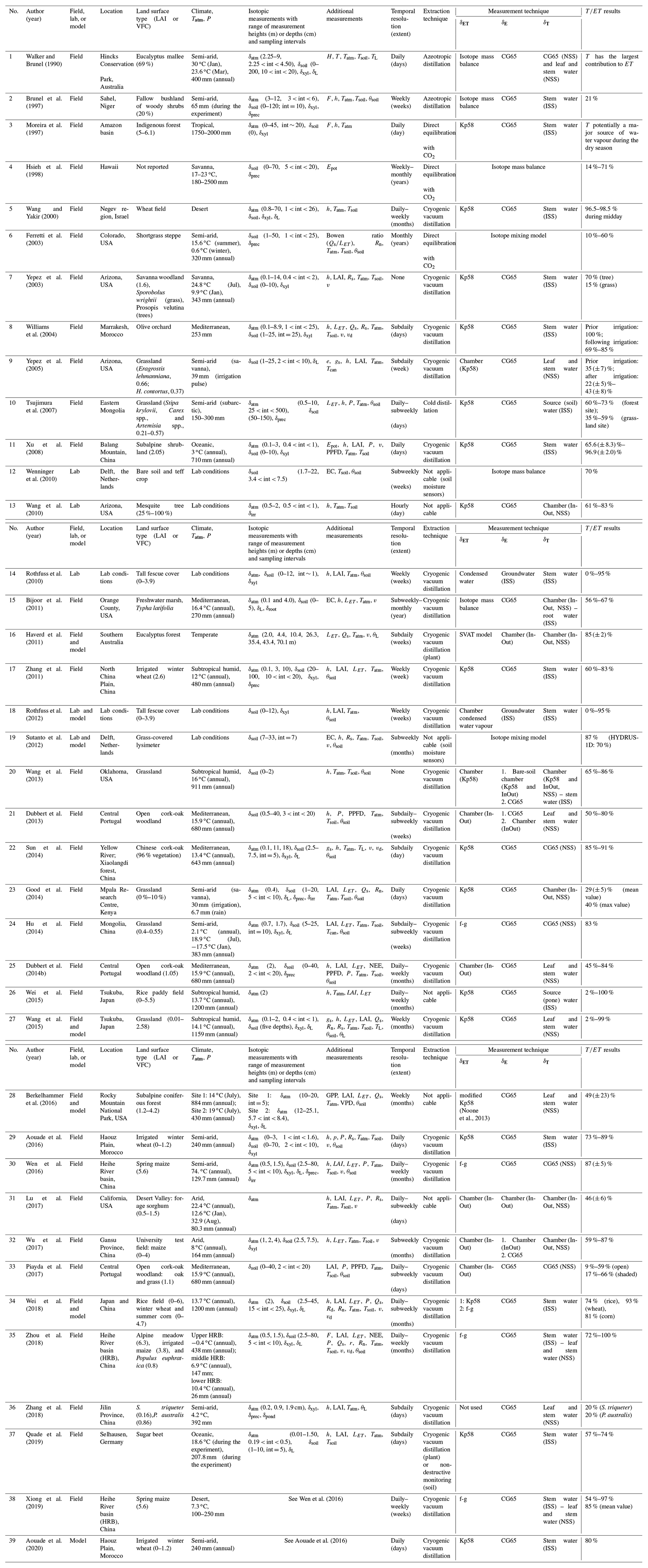
| Symbol or abbreviation | Description | Dimension or unit |
| Catm, Cbg, CET | Atmospheric and background water vapour concentration, rise in atmospheric water vapour concentration due to evapotranspiration flux | M L−3 |
| E,ELys,Epot | Soil evaporation rate, soil evaporation (micro-lysimeter), potential evaporation | L3 T−1 |
| EC | Eddy covariance | |
| ET | Evapotranspiration rate | L3 T−1 |
| f | Measurement frequency | T−1 |
| FET, jFET, iFE, FE, jFE, jFT, iFT, jFxyl, iFxyl | Evapotranspiration water vapour flux density rate, evapotranspiration, evaporation, transpiration, and xylem water flux density rates of the rare (i) and abundant (j) isotopologue | |
| gs | Leaf stomatal conductance | |
| GPP | Gross primary production | |
| hatm,hEF | Atmospheric relative humidity and soil pore space relative humidity at the evaporating front | – |
| K | Eddy diffusivity of water vapour | L2 T−1 |
| LAI | Leaf area index | L2 L−2 |
| LET | Latent heat flux of evapotranspiration | M T−3 |
| Matm, Mw | Molecular weight of dry air and water | M L−3 |
| n | Adimensional factor accounting for flow conditions above the liquid water–water vapour equilibrium layer | – |
| NEE | Net ecosystem exchange | |
| P | Precipitation amount | L3 L−2 |
| p | Proportion of leaf water in isotopic equilibrium with water vapour in the stomatal cavity | – |
| PPFD | Photosynthetic photon flux density | |
| Qs | Sensible heat flux | M T−3 |
| R | Universal gas constant | |
| Rstd, REF, Rsat | Isotopic ratio of the Vienna Standard Mean Ocean Water (V-SMOW), soil water at the evaporating front, and saturated water vapour | – |
| Rn, Rs, Rd | Net and solar radiation and radiation flux density | M T−3 |
| Rgas | Universal gas constant | |
| jr, ir jD, iD | Bulk resistances to vapour transport of the rare (i) and abundant (j) isotopologuesMolecular diffusivities of the rare (i) and abundant (j) water vapour isotopologues | |
| S | Sap-flux density | |
| T | Transpiration rate | L3 T−1 |
| Tatm, Tsoil, TEF, TL, Tcan | Temperature of the atmosphere, soil, soil at the evaporating front, leaf surface, and canopy atmosphere | ∘C |
| Transpiration fraction | – | |
| uin, uout | Flow rate measured at the inlet and outlet of a gas exchange chamber | L3 T−1 |
| v (vd) | Wind speed (wind direction) | L T−1 |
| VFC | Vegetation fractional coverage | L2 L−2 |
| VPD | Vapour pressure deficit | P |
| z, zatm, zEF | Vertical coordinate, atmospheric height, and soil evaporating front depth | M |
| αeq αK | Equilibrium isotopic fractionation factorKinetic-isotopic-fractionation factor | – |
| δatm, δsoil, , δL, δxyl, δprec, δroot, δirr, δpond, δin, δout | Isotopic composition of the atmospheric water vapour, soil water, soil water vapour, leaf water, xylem water, precipitation, root water, irrigation water, pond water, and water vapour measured at the inlet and outlet of a gas exchange chamber | – |
| εeq εK | Equilibrium isotopic fractionationKinetic isotopic fractionation | – |
| φ | Isotope analyser inlet flow rate | L3 T−1 |
| ρatm, ρw | Volumetric mass of dry air and water | M L−3 |
| Soil, soil surface, soil residual, and soil saturated water content, leaf water content | L3 L−3 | |
| τL | Leaf water turnover time | T |
| χatm, χbg, jχatm, iχatm, , , χET, χin, χout | Atmospheric and background water vapour mixing ratio, water vapour mixing ratio of the rare (i) and abundant (j) isotope, saturated water vapour mixing ratio of the rare (i) and abundant (j) isotope, rise in atmospheric water vapour mixing ratio due to evapotranspiration flux, water vapour mixing ratio measured at the inlet and outlet of a gas exchange chamber | L3 L−3 |
| ψEF | Soil water matric potential at the evaporating front |
Data used in Fig. 2 can be consulted in Table A1. Details about the calculation of the isotopic composition of evaporation (Sect. 3.2.2) are given in Table 1. Data supporting Figs. 1, 4, and 6 are synthetic and were not attributed to specific DOIs; these are available upon request from the authors.
YR, MQ, and MD reviewed the published literature and prepared the manuscript. All authors reviewed the manuscript.
The authors declare that they have no conflict of interest.
Youri Rothfuss and Maren Dubbert acknowledge funding by the German Science Foundation (DFG, grant nos. RO 5421/1-1 and DU1688/1-1). Maria Quade was funded by the German Ministry of Education and Research (BMBF) within the project IDAS-GHG (Instrumental and Data-driven Approaches to Source Partitioning of Greenhouse Gas Fluxes: Comparison, Combination, Advancement, grant no. 01LN1313A).
This research has been supported by the IDAS-GHG project (Instrumental and Data-driven Approaches to Source Partitioning of Greenhouse Gas Fluxes: Comparison, Combination, Advancement, grant no. 01LN1313A).
The article processing charges for this open-access
publication were covered by a Research
Centre of the Helmholtz Association.
This paper was edited by Ivonne Trebs and reviewed by John Marshall and one anonymous referee.
Allen, S. T., Keim, R. F., Barnard, H. R., McDonnell, J. J., and Brooks, J. R.: The role of stable isotopes in understanding rainfall interception processes: a review, Wiley Interdisciplinary Reviews-Water, 4, 1–17, https://doi.org/10.1002/wat2.1187, 2017.
Allison, G. B.: The relationship between 18O and deuterium in water in sand columns undergoing evaporation, J. Hydrol., 55, 163–169, https://doi.org/10.1016/0022-1694(82)90127-5, 1982.
Alton, P., Fisher, R., Los, S., and Williams, M.: Simulations of global evapotranspiration using semiempirical and mechanistic schemes of plant hydrology, Global Biogeochem. Cy., 23, Gb4023, https://doi.org/10.1029/2009gb003540, 2009.
Anderson, R. G., Zhang, X. D., and Skaggs, T. H.: Measurement and partitioning of evapotranspiration for application to vadose zone studies, Vadose Zone J., 16, 1–9, https://doi.org/10.2136/vzj2017.08.0155, 2017.
Aouade, G., Ezzahar, J., Amenzou, N., Er-Raki, S., Benkaddour, A., Khabba, S., and Jarlan, L.: Combining stable isotopes, Eddy Covariance system and meteorological measurements for partitioning evapotranspiration, of winter wheat, into soil evaporation and plant transpiration in a semi-arid region, Agr. Water Manage., 177, 181–192, https://doi.org/10.1016/j.agwat.2016.07.021, 2016.
Aouade, G., Jarlan, L., Ezzahar, J., Er-Raki, S., Napoly, A., Benkaddour, A., Khabba, S., Boulet, G., Garrigues, S., Chehbouni, A., and Boone, A.: Evapotranspiration partition using the multiple energy balance version of the land surface model over two irrigated crops in a semi-arid Mediterranean region (Marrakech, Morocco), Hydrol. Earth Syst. Sci., 24, 3789–3814, https://doi.org/10.5194/hess-24-3789-2020, 2020.
Araguás-Araguás, L., Rozanski, K., Gonfiantini, R., and Louvat, D.: Isotope effects accompanying vacuum extraction of soil-water for stable-isotope analyses, J. Hydrol., 168, 159–171, https://doi.org/10.1016/0022-1694(94)02636-P, 1995.
Baldocchi, D.: Measuring fluxes of trace gases and energy between ecosystems and the atmosphere – the state and future of the eddy covariance method, Glob. Change Biol., 20, 3600–3609, https://doi.org/10.1111/gcb.12649, 2014.
Barbeta, A., Jones, S. P., Clavé, L., Wingate, L., Gimeno, T. E., Fréjaville, B., Wohl, S., and Ogée, J.: Unexplained hydrogen isotope offsets complicate the identification and quantification of tree water sources in a riparian forest, Hydrol. Earth Syst. Sci., 23, 2129–2146, https://doi.org/10.5194/hess-23-2129-2019, 2019.
Bariac, T., Klamecki, A., Jusserand, C., and Létolle, R.: Isotopic composition (18O) of water in the continuum soil-plant atmosphere (an example in a wheat crop experimental site at Versailles, France, June 1984) Catena, 14, 55–72, 1987.
Bariac, T., Gonzalezdunia, J., Tardieu, F., Tessier, D., and Mariotti, A.: Spatial variation of the isotopic composition of water (18O, 2H) in organs of aerophytic plants. 1. Assessment under laboratory conditions, Chem. Geol., 115, 307–315, https://doi.org/10.1016/0009-2541(94)90194-5, 1994.
Barnes, C. J. and Allison, G. B.: The distribution of deuterium and 18O in dry Soils. 1. Theory, J. Hydrol., 60, 141–156, https://doi.org/10.1016/0022-1694(83)90018-5, 1983.
Barnes, C. J. and Allison, G. B.: Tracing of water-movement in the unsaturated zone using stable isotopes of hydrogen and oxygen, J. Hydrol., 100, 143–176, https://doi.org/10.1016/0022-1694(88)90184-9, 1988.
Barnes, C. J. and Walker, G. R.: The distribution of deuterium and 18O during unsteady evaporation from a dry soil, J. Hydrol., 112, 55–67, https://doi.org/10.1016/0022-1694(89)90180-7, 1989.
Barron-Gafford, G. A., Grieve, K. A., and Murthy, R.: Leaf- and stand-level responses of a forested mesocosm to independent manipulations of temperature and vapor pressure deficit, New Phytol., 174, 614–625, https://doi.org/10.1111/j.1469-8137.2007.02035.x, 2007.
Berkelhammer, M., Noone, D. C., Wong, T. E., Burns, S. P., Knowles, J. F., Kaushik, A., Blanken, P. D., and Williams, M. W.: Convergent approaches to determine an ecosystem's transpiration fraction, Global Biogeochem. Cy., 30, 933–951, https://doi.org/10.1002/2016gb005392, 2016.
Beyer, M., Kühnhammer, K., and Dubbert, M.: In situ measurements of soil and plant water isotopes: a review of approaches, practical considerations and a vision for the future, Hydrol. Earth Syst. Sci., 24, 4413–4440, https://doi.org/10.5194/hess-24-4413-2020, 2020.
Bijoor, N. S., Pataki, D. E., Rocha, A. V., and Goulden, M. L.: The application of δ18O and delta δD for understanding water pools and fluxes in a Typha marsh, Plant Cell Environ., 34, 1761–1775, https://doi.org/10.1111/j.1365-3040.2011.02372.x, 2011.
Braden-Behrens, J., Markwitz, C., and Knohl, A.: Eddy covariance measurements of the dual-isotope composition of evapotranspiration, Agr. Forest Meteorol., 269, 203–219, https://doi.org/10.1016/j.agrformet.2019.01.035, 2019.
Braden-Behrens, J., Siebicke, L., and Knohl, A.: Drivers of the variability of the isotopic composition of water vapor in the surface boundary layer, Biogeosciences Discuss. [preprint], https://doi.org/10.5194/bg-2020-398, in review, 2020.
Braud, I., Bariac, T., Gaudet, J. P., and Vauclin, M.: SiSPAT-Isotope, a coupled heat, water and stable isotope (HDO and ) transport model for bare soil. Part I. Model description and first verifications, J. Hydrol., 309, 277–300, https://doi.org/10.1016/j.jhydrol.2004.12.013, 2005.
Braud, I., Biron, P., Bariac, T., Richard, P., Canale, L., Gaudet, J. P., and Vauclin, M.: Isotopic composition of bare soil evaporated water vapor. Part I: RUBIC IV experimental setup and results, J. Hydrol., 369, 1–16, https://doi.org/10.1016/j.jhydrol.2009.01.034, 2009.
Brunel, J. P., Walker, G. R., Dighton, J. C., and Monteny, B.: Use of stable isotopes of water to determine the origin of water used by the vegetation and to partition evapotranspiration. A case study from HAPEX-Sahel, J. Hydrol., 189, 466–481, 1997.
Brutsaert, W.: Theory for local evaporation (or heat-transfer) from rough and smooth surfaces at ground level, Water Resour. Res., 11, 543–550, https://doi.org/10.1029/WR011i004p00543, 1975.
Cernusak, L. A., Pate, J. S., and Farquhar, G. D.: Diurnal variation in the stable isotope composition of water and dry matter in fruiting Lupinus angustifolius under field conditions, Plant Cell Environ., 25, 893–907, https://doi.org/10.1046/j.1365-3040.2002.00875.x, 2002.
Cernusak, L. A., Farquhar, G. D., and Pate, J. S.: Environmental and physiological controls over oxygen and carbon isotope composition of Tasmanian blue gum, Eucalyptus globulus, Tree Physiol., 25, 129–146, 2005.
Chen, Y., Helliker, B. R., Tang, X., Li, F., Zhou, Y., and Song, X.: Stem water cryogenic extraction biases estimation in deuterium isotope composition of plant source water, P. Natl. Acad. Sci. USA, 117, 33345–33350, https://doi.org/10.1073/pnas.2014422117, 2020.
Craig, H. and Gordon, L. I.: Deuterium and oxygen 18 variations in the ocean and marine atmosphere, in: Stable Isotopes in Oceanographic Studies and Paleotemperatures, Spoleto, Italy, 1965, 9–130, 1965.
Cuntz, M., Ogee, J., Farquhar, G. D., Peylin, P., and Cernusak, L. A.: Modelling advection and diffusion of water isotopologues in leaves, Plant Cell Environ., 30, 892–909, https://doi.org/10.1111/j.1365-3040.2007.01676.x, 2007.
Dongmann, G., Nurnberg, H. W., Forstel, H., and Wagener, K.: On the enrichment of in leaves of transpiring plants, Radiat. Environ. Bioph., 11, 41–52, https://doi.org/10.1007/Bf01323099, 1974.
Dubbert, M. and Werner, C.: Water fluxes mediated by vegetation: emerging isotopic insights at the soil and atmosphere interfaces, New Phytol., 221, 1754–1763, https://doi.org/10.1111/nph.15547, 2019.
Dubbert, M., Cuntz, M., Piayda, A., Maguás, C., and Werner, C.: Partitioning evapotranspiration – Testing the Craig and Gordon model with field measurements of oxygen isotope ratios of evaporative fluxes, J. Hydrol., 496, 142–153, https://doi.org/10.1016/j.jhydrol.2013.05.033, 2013.
Dubbert, M., Cuntz, M., Piayda, A., and Werner, C.: Oxygen isotope signatures of transpired water vapor – the role of isotopic non-steady-state transpiration under natural conditions, New Phytol., 203, 1242–1252, https://doi.org/10.1111/nph.12878, 2014a.
Dubbert, M., Piayda, A., Cuntz, M., Correia, A. C., Costa E Silva, F., Pereira, J. S., and Werner, C.: Stable oxygen isotope and flux partitioning demonstrates understory of an oak savanna contributes up to half of ecosystem carbon and water exchange, Front. Plant Sci., 5, 530, https://doi.org/10.3389/fpls.2014.00530, 2014b.
Dubbert, M., Kübert, A., and Werner, C.: Impact of leaf traits on temporal dynamics of transpired oxygen isotope signatures and its impact on atmospheric vapor, Font. Plant Sci., 8, 5, https://doi.org/10.3389/fpls.2017.00005, 2017.
Ellsworth, P. Z. and Williams, D. G.: Hydrogen isotope fractionation during water uptake by woody xerophytes, Plant Soil, 291, 93–107, https://doi.org/10.1007/s11104-006-9177-1, 2007.
Farquhar, G. D. and Cernusak, L. A.: On the isotopic composition of leaf water in the non-steady state, Funct. Plant Biol., 32, 293–303, https://doi.org/10.1071/Fp04232, 2005.
Farquhar, G. D., Hubick, K. T., Condon, A. G., and Richards, R. A.: Carbon isotope discrimination and water-use efficiency, in: Stable Isotopes in Ecological Research, edited by: Rundel, P. W., Ehleringer, J. R., and Nagy, K. A., Springer-Verlag, New York, pp 21–46, 1989.
Farquhar, G. D., Cernusak, L. A., and Barnes, B.: Heavy water fractionation during transpiration, Plant Physiol., 143, 11–18, https://doi.org/10.1104/pp.106.093278, 2007.
Ferretti, D. F., Pendall, E., Morgan, J. A., Nelson, J. A., LeCain, D., and Mosier, A. R.: Partitioning evapotranspiration fluxes from a Colorado grassland using stable isotopes: Seasonal variations and ecosystem implications of elevated atmospheric CO2, Plant Soil, 254, 291–303, https://doi.org/10.1023/A:1025511618571, 2003.
Flanagan, L. B., Comstock, J. P., and Ehleringer, J. R.: Comparison of modeled and observed environmental-influences on the stable oxygen and hydrogen isotope composition of leaf water in Phaseolus-Vulgaris L., Plant Physiol., 96, 588–596, https://doi.org/10.1104/pp.96.2.588, 1991.
Gaj, M., Beyer, M., Koeniger, P., Wanke, H., Hamutoko, J., and Himmelsbach, T.: In situ unsaturated zone water stable isotope (2H and 18O) measurements in semi-arid environments: a soil water balance, Hydrol. Earth Syst. Sci., 20, 715–731, https://doi.org/10.5194/hess-20-715-2016, 2016.
Gangi, L., Rothfuss, Y., Ogee, J., Wingate, L., Vereecken, H., and Bruggemann, N.: A new method for in situ measurements of oxygen isotopologues of soil water and carbon dioxide with high time resolution, Vadose Zone J., 14, 1–14, https://doi.org/10.2136/vzj2014.11.0169, 2015.
Garvelmann, J., Külls, C., and Weiler, M.: A porewater-based stable isotope approach for the investigation of subsurface hydrological processes, Hydrol. Earth Syst. Sci., 16, 631–640, https://doi.org/10.5194/hess-16-631-2012, 2012.
Gat, J. R.: Atmospheric water balance – the isotopic perspective, Hydrol. Process., 14, 1357–1369, https://doi.org/10.1002/1099-1085(20000615)14:8<1357::Aid-Hyp986>3.0.Co;2-7, 2000.
Gonfiantini, R.: Standards for stable isotope measurements in natural compounds, Nature, 271, 534–536, https://doi.org/10.1038/271534a0, 1978.
Good, S. P., Soderberg, K., Wang, L. X., and Caylor, K. K.: Uncertainties in the assessment of the isotopic composition of surface fluxes: A direct comparison of techniques using laser-based water vapor isotope analyzers, J. Geophys. Res.-Atmos., 117, D15301, https://doi.org/10.1029/2011jd017168, 2012.
Good, S. P., Soderberg, K., Guan, K. Y., King, E. G., Scanlon, T. M., and Caylor, K. K.: δ2H isotopic flux partitioning of evapotranspiration over a grass field following a water pulse and subsequent dry down, Water Resour. Res., 50, 1410–1432, https://doi.org/10.1002/2013WR014333, 2014.
Good, S. P., Noone, D., and Bowen, G.: Hydrologic connectivity constrains partitioning of global terrestrial water fluxes, Science, 349, 175–177, https://doi.org/10.1126/science.aaa5931, 2015.
Griffis, T. J.: Tracing the flow of carbon dioxide and water vapor between the biosphere and atmosphere: A review of optical isotope techniques and their application, Agr. Forest Meteorol., 174, 85–109, https://doi.org/10.1016/j.agrformet.2013.02.009, 2013.
Griffis, T. J., Lee, X., Baker, J. M., Sargent, S. D., and King, J. Y.: Feasibility of quantifying ecosystem-atmosphere C18O16C exchange using laser spectroscopy and the flux-gradient method, Agr. Forest Meteorol., 135, 44–60, https://doi.org/10.1016/j.agrformet.2005.10.002, 2005.
Griffis, T. J., Sargent, S. D., Lee, X., Baker, J. M., Greene, J., Erickson, M., Zhang, X., Billmark, K., Schultz, N., Xiao, W., and Hu, N.: Determining the oxygen isotope composition of evapotranspiration using eddy covariance, Bound.-Lay. Meteorol., 137, 307–326, https://doi.org/10.1007/s10546-010-9529-5, 2010.
Griffis, T. J., Lee, X., Baker, J. M., Billmark, K., Schultz, N., Erickson, M., Zhang, X., Fassbinder, J., Xiao, W., and Hu, N.: Oxygen isotope composition of evapotranspiration and its relation to C-4 photosynthetic discrimination, J. Geophys. Res.-Biogeo., 116, G01035, https://doi.org/10.1029/2010jg001514, 2011.
Groh, J., Stumpp, C., Lucke, A., Putz, T., Vanderborght, J., and Vereecken, H.: Inverse Estimation of Soil Hydraulic and Transport Parameters of Layered Soils from Water Stable Isotope and Lysimeter Data, Vadose Zone J., 17, 1–19, https://doi.org/10.2136/vzj2017.09.0168, 2018.
Haverd, V. and Cuntz, M.: Soil-Litter-Iso: A one-dimensional model for coupled transport of heat, water and stable isotopes in soil with a litter layer and root extraction, J. Hydrol., 388, 438–455, https://doi.org/10.1016/j.jhydrol.2010.05.029, 2010.
Haverd, V., Cuntz, M., Griffith, D., Keitel, C., Tadros, C., and Twining, J.: Measured deuterium in water vapour concentration does not improve the constraint on the partitioning of evapotranspiration in a tall forest canopy, as estimated using a soil vegetation atmosphere transfer model, Agr. Forest Meteorol., 151, 645–654, https://doi.org/10.1016/j.agrformet.2011.02.005, 2011.
Havranek, R. E., Snell, K. E., Davidheiser-Kroll, B., Bowen, G. J., and Vaughn, B.: The Soil Water Isotope Storage System (SWISS): An integrated soil water vapor sampling and multiport storage system for stable isotope geochemistry, Rapid Commun. Mass Sp., 34, e8783, https://doi.org/10.1002/rcm.8783, 2020.
Hollinger, D. Y. and Richardson, A. D.: Uncertainty in eddy covariance measurements and its application to physiological models, Tree Physiol., 25, 873–885, https://doi.org/10.1093/treephys/25.7.873, 2005.
Horita, J. and Wesolowski, D. J.: Liquid-vapor fractionation of oxygen and hydrogen isotopes of water from the freezing to the critical-temperature, Geochim. Cosmochim. Ac., 58, 3425–3437, https://doi.org/10.1016/0016-7037(94)90096-5, 1994.
Horita, J., Rozanski, K., and Cohen, S.: Isotope effects in the evaporation of water: a status report of the Craig–Gordon model, Isot. Environ. Health S., 44, 23–49, https://doi.org/10.1080/10256010801887174, 2008.
Hsieh, J. C. C., Chadwick, O. A., Kelly, E. F., and Savin, S. M.: Oxygen isotopic composition of soil water: Quantifying evaporation and transpiration, Geoderma, 82, 269–293, https://doi.org/10.1016/S0016-7061(97)00105-5, 1998.
Hu, Y., Xiao, W., Wei, Z., Welp, L., Wen, X., and Lee, X.: Determining the isotopic composition of surface water vapor flux from high-frequency observations using flux-gradient and Keeling plot methods, Earth and Space Science, 8, e2020EA001304, https://doi.org/10.1002/es-soar.10501239.1, 2020.
Hu, Z. M., Wen, X. F., Sun, X. M., Li, L. H., Yu, G. R., Lee, X. H., and Li, S. G.: Partitioning of evapotranspiration through oxygen isotopic measurements of water pools and fluxes in a temperate grassland, J. Geophys. Res.-Biogeo., 119, 358–371, https://doi.org/10.1002/2013jg002367, 2014.
Humphrey, V., Zscheischler, J., Ciais, P., Gudmundsson, L., Sitch, S., and Seneviratne, S. I.: Sensitivity of atmospheric CO2 growth rate to observed changes in terrestrial water storage, Nature, 560, 628–631, https://doi.org/10.1038/s41586-018-0424-4, 2018.
Ito, A. and Inatomi, M.: Water-use efficiency of the terrestrial biosphere: a model analysis focusing on interactions between the global carbon and water cycles, J. Hydrometeorol., 13, 681–694, https://doi.org/10.1175/Jhm-D-10-05034.1, 2012.
Jarvis, P. G.: Interpretation of variations in leaf water potential and stomatal conductance found in canopies in field, Philos. T. R. Soc. B, 273, 593–610, https://doi.org/10.1098/rstb.1976.0035, 1976.
Jasechko, S., Sharp, Z. D., Gibson, J. J., Birks, S. J., Yi, Y., and Fawcett, P. J.: Terrestrial water fluxes dominated by transpiration, Nature, 496, 347–350, https://doi.org/10.1038/Nature11983, 2013.
Keeling, C. D.: The concentration and isotopic abundances of atmospheric carbon dioxide in rural areas, Geochim. Cosmochim. Ac., 13, 322–334, https://doi.org/10.1016/0016-7037(58)90033-4, 1958.
Kelliher, F. M., Kostner, B. M. M., Hollinger, D. Y., Byers, J. N., Hunt, J. E., Mcseveny, T. M., Meserth, R., Weir, P. L., and Schulze, E. D.: Evaporation, xylem sap flow, and tree transpiration in a New-Zealand broad-leaved Forest, Agr. Forest Meteorol., 62, 53–73, https://doi.org/10.1016/0168-1923(92)90005-O, 1992.
Kelln, C. J., Wassenaar, L. I., and Hendry, M. J.: Stable isotopes (δ18O, δ2H) of pore waters in clay-rich aquitards: A comparison and evaluation of measurement techniques, Ground Water Monit. R., 21, 108–116, https://doi.org/10.1111/j.1745-6592.2001.tb00306.x, 2001.
Kool, D., Agam, N., Lazarovitch, N., Heitman, J. L., Sauer, T. J., and Ben-Gal, A.: A review of approaches for evapotranspiration partitioning, Agr. Forest Meteorol., 184, 56–70, https://doi.org/10.1016/j.agrformet.2013.09.003, 2014.
Kübert, A., Paulus, S., Dahlmann, A., Werner, C., Rothfuss, Y., and Orlowski, N.: Water stable isotopes in ecohydrological field research: comparison between In situ and destructive monitoring methods to determine soil water isotopic signatures, Front. Plant Sci., 11, 387, https://doi.org/10.3389/fpls.2020.00387, 2020.
Kühnhammer, K., Kübert, A., Brüggemann, N., Deseano Diaz, P., van Dusschoten, D., Javaux, M., Merz, S., Vereecken, H., Dubbert, M., and Rothfuss, Y.: Investigating the root plasticity response of Centaurea jacea to soil water availability changes from isotopic analysis, New Phytol., 226, 98–110, https://doi.org/10.1111/nph.16352, 2019.
Law, B. E., Falge, E., Gu, L., Baldocchi, D. D., Bakwin, P., Berbigier, P., Davis, K., Dolman, A. J., Falk, M., Fuentes, J. D., Goldstein, A., Granier, A., Grelle, A., Hollinger, D., Janssens, I. A., Jarvis, P., Jensen, N. O., Katul, G., Mahli, Y., Matteucci, G., Meyers, T., Monson, R., Munger, W., Oechel, W., Olson, R., Pilegaard, K., Paw, K. T., Thorgeirsson, H., Valentini, R., Verma, S., Vesala, T., Wilson, K., and Wofsy, S.: Environmental controls over carbon dioxide and water vapor exchange of terrestrial vegetation, Agr. Forest Meteorol., 113, 97–120, https://doi.org/10.1016/S0168-1923(02)00104-1, 2002.
Lawrence, D. M., Thornton, P. E., Oleson, K. W., and Bonan, G. B.: The partitioning of evapotranspiration into transpiration, soil evaporation, and canopy evaporation in a GCM: Impacts on land-atmosphere interaction, J. Hydrometeorol., 8, 862–880, https://doi.org/10.1175/Jhm596.1, 2007.
Lee, H., Smith, R., and Williams, J.: Water vapour 18O/16O isotope ratio in surface air in New England, USA, Tellus B, 58, 293–304, https://doi.org/10.1111/j.1600-0889.2006.00191.x, 2006.
Lee, X., Huang, J. P., and Patton, E. G.: A large-Eddy simulation study of water vapour and carbon dioxide isotopes in the atmospheric boundary layer, Bound.-Lay. Meteorol., 145, 229–248, https://doi.org/10.1007/s10546-011-9631-3, 2012.
Lee, X. H., Kim, K., and Smith, R.: Temporal variations of the 18O/16O signal of the whole-canopy transpiration in a temperate forest, Global Biogeochem. Cy., 21, GB3013, https://doi.org/10.1029/2006gb002871, 2007.
Lee, X. H., Griffis, T. J., Baker, J. M., Billmark, K. A., Kim, K., and Welp, L. R.: Canopy-scale kinetic fractionation of atmospheric carbon dioxide and water vapor isotopes, Global Biogeochem. Cy., 23, GB3013, https://doi.org/10.1029/2008gb003331, 2009.
Loescher, H. W., Law, B. E., Mahrt, L., Hollinger, D. Y., Campbell, J., and Wofsy, S. C.: Uncertainties in, and interpretation of, carbon flux estimates using the eddy covariance technique, J. Geophys. Res.-Atmos., 111, D21S90, https://doi.org/10.1029/2005jd006932, 2006.
Longdoz, B., Yernaux, M., and Aubinet, M.: Soil CO2 efflux measurements in a mixed forest: impact of chamber disturbances, spatial variability and seasonal evolution, Glob. Change Biol., 6, 907–917, https://doi.org/10.1046/j.1365-2486.2000.00369.x, 2000.
Lu, X. F., Liang, L. Y. L., Wang, L. X., Jenerette, G. D., McCabe, M. F., and Grantz, D. A.: Partitioning of evapotranspiration using a stable isotope technique in an arid and high temperature agricultural production system, Agr. Water Manage., 179, 103–109, https://doi.org/10.1016/j.agwat.2016.08.012, 2017.
Luz, B., Barkan, E., Yam, R., and Shemesh, A.: Fractionation of oxygen and hydrogen isotopes in evaporating water, Geochim. Cosmochim. Ac., 73, 6697–6703, https://doi.org/10.1016/j.gca.2009.08.008, 2009.
Marshall, J. D., Cuntz, M., Beyer, M., Dubbert, M., and Kühnhammer, K.: Borehole Equilibration: Testing a new method to monitor the isotopic composition of tree xylem water in situ, Front. Plant Sci., 11, 358, https://doi.org/10.3389/fpls.2020.00358, 2020.
Masson, V., Le Moigne, P., Martin, E., Faroux, S., Alias, A., Alkama, R., Belamari, S., Barbu, A., Boone, A., Bouyssel, F., Brousseau, P., Brun, E., Calvet, J.-C., Carrer, D., Decharme, B., Delire, C., Donier, S., Essaouini, K., Gibelin, A.-L., Giordani, H., Habets, F., Jidane, M., Kerdraon, G., Kourzeneva, E., Lafaysse, M., Lafont, S., Lebeaupin Brossier, C., Lemonsu, A., Mahfouf, J.-F., Marguinaud, P., Mokhtari, M., Morin, S., Pigeon, G., Salgado, R., Seity, Y., Taillefer, F., Tanguy, G., Tulet, P., Vincendon, B., Vionnet, V., and Voldoire, A.: The SURFEXv7.2 land and ocean surface platform for coupled or offline simulation of earth surface variables and fluxes, Geosci. Model Dev., 6, 929–960, https://doi.org/10.5194/gmd-6-929-2013, 2013.
Mathieu, R., and Bariac, T.: A numerical model for the simulation of stable isotope profiles in drying soils, J. Geophys. Res.-Atmos., 101, 12685–12696, https://doi.org/10.1029/96jd00223, 1996.
Mayer, J. C., Hens, K., Rummel, U., Meixner, F. X., and Foken, T.: Moving measurement platforms – specific challenges and corrections, Meteorol. Z., 18, 477–488, https://doi.org/10.1127/0941-2948/2009/0401, 2009.
Merlivat, L.: Molecular diffusivities of , HD16O, and in gases, J. Chem. Phys., 69, 2864–2871, https://doi.org/10.1063/1.436884, 1978.
Merz, S., Balcom, B. J., Enjilela, R., Vanderborght, J., Rothfuss, Y., Vereecken, H., and Pohlmeier, A.: Magnetic resonance monitoring and numerical modeling of soil moisture during evaporation, Vadose Zone J., 17, 1–15, https://doi.org/10.2136/vzj2016.10.0099, 2018.
Millar, C., Pratt, D., Schneider, D. J., and McDonnell, J. J.: A comparison of extraction systems for plant water stable isotope analysis, Rapid Commun. Mass Sp., 32, 1031–1044, https://doi.org/10.1002/rcm.8136, 2018.
Moreira, M. Z., Sternberg, L. D. L., Martinelli, L. A., Victoria, R. L., Barbosa, E. M., Bonates, L. C. M., and Nepstad, D. C.: Contribution of transpiration to forest ambient vapour based on isotopic measurements, Glob. Change Biol., 3, 439–450, https://doi.org/10.1046/j.1365-2486.1997.00082.x, 1997.
Mubarak, A. and Olsen, R. A.: Immiscible displacement of soil solution by centrifugation, Soil Sci. Soc. Am. J., 40, 329–331, 1976.
Munksgaard, N. C., Cheesman, A. W., Wurster, C. M., Cernusak, L. A., and Bird, M. I.: Microwave extraction-isotope ratio infrared spectroscopy (ME-IRIS): a novel technique for rapid extraction and in-line analysis of δ18O and δ2H values of water in plants, soils and insects, Rapid Commun. Mass Sp., 28, 2151–2161, https://doi.org/10.1002/rcm.7005, 2014.
Ney, P. and Graf, A.: High-Resolution vertical profile measurements for carbon dioxide and water vapour concentrations within and above crop canopies, Bound.-Lay. Meteorol., 166, 449–473, https://doi.org/10.1007/s10546-017-0316-4, 2018.
Noone, D., Risi, C., Bailey, A., Berkelhammer, M., Brown, D. P., Buenning, N., Gregory, S., Nusbaumer, J., Schneider, D., Sykes, J., Vanderwende, B., Wong, J., Meillier, Y., and Wolfe, D.: Determining water sources in the boundary layer from tall tower profiles of water vapor and surface water isotope ratios after a snowstorm in Colorado, Atmos. Chem. Phys., 13, 1607–1623, https://doi.org/10.5194/acp-13-1607-2013, 2013.
Oerter, E. and Bowen, G.: Spatio-temporal heterogeneity in soil water stable isotopic composition and its ecohydrologic implications in semiarid ecosystems, Hydrol. Process., 33, 1724–1738, https://doi.org/10.1002/hyp.13434, 2019.
Oerter, E. J., Perelet, A., Pardyjak, E., and Bowen, G.: Membrane inlet laser spectroscopy to measure H and O stable isotope compositions of soil and sediment pore water with high sample throughput, Rapid Commun. Mass Sp., 31, 75–84, https://doi.org/10.1002/rcm.7768, 2017.
Or, D., Lehmann, P., Shahraeeni, E., and Shokri, N.: Advances in soil evaporation physics-A review, Vadose Zone J., 12, 1–16, https://doi.org/10.2136/vzj2012.0163, 2013.
Orlowski, N., Breuer, L., and McDonnell, J. J.: Critical issues with cryogenic extraction of soil water for stable isotope analysis, Ecohydrology, 9, 3–10, https://doi.org/10.1002/eco.1722, 2016a.
Orlowski, N., Pratt, D. L., and McDonnell, J. J.: Intercomparison of soil pore water extraction methods for stable isotope analysis, Hydrol. Process., 30, 3434–3449, https://doi.org/10.1002/hyp.10870, 2016b.
Orlowski, N., Breuer, L., Angeli, N., Boeckx, P., Brumbt, C., Cook, C. S., Dubbert, M., Dyckmans, J., Gallagher, B., Gralher, B., Herbstritt, B., Hervé-Fernández, P., Hissler, C., Koeniger, P., Legout, A., Macdonald, C. J., Oyarzún, C., Redelstein, R., Seidler, C., Siegwolf, R., Stumpp, C., Thomsen, S., Weiler, M., Werner, C., and McDonnell, J. J.: Inter-laboratory comparison of cryogenic water extraction systems for stable isotope analysis of soil water, Hydrol. Earth Syst. Sci., 22, 3619–3637, https://doi.org/10.5194/hess-22-3619-2018, 2018.
Pataki, D. E., Ehleringer, J. R., Flanagan, L. B., Yakir, D., Bowling, D. R., Still, C. J., Buchmann, N., Kaplan, J. O., and Berry, J. A.: The application and interpretation of Keeling plots in terrestrial carbon cycle research, Global Biogeochem. Cy., 17, 1022, https://doi.org/10.1029/2001gb001850, 2003.
Phillips, D. L. and Gregg, J. W.: Uncertainty in source partitioning using stable isotopes, Oecologia, 127, 171–179, https://doi.org/10.1007/s004420000578, 2001.
Phillips, D. L. and Gregg, J. W.: Source partitioning using stable isotopes: Coping with too many sources, Oecologia, 136, 261–269, https://doi.org/10.1007/s00442-003-1218-3, 2003.
Piayda, A., Dubbert, M., Siegwolf, R., Cuntz, M., and Werner, C.: Quantification of dynamic soil–vegetation feedbacks following an isotopically labelled precipitation pulse, Biogeosciences, 14, 2293–2306, https://doi.org/10.5194/bg-14-2293-2017, 2017.
Quade, M., Bruggemann, N., Graf, A., Vanderborght, J., Vereecken, H., and Rothfuss, Y.: Investigation of kinetic isotopic fractionation of water during bare soil evaporation, Water Resour. Res., 54, 6909–6928, https://doi.org/10.1029/2018wr023159, 2018.
Quade, M., Klosterhalfen, A., Graf, A., Brüggemann, N., Hermes, N., Vereecken, H., and Rothfuss, Y.: In-situ monitoring of soil water isotopic composition for partitioning of evapotranspiration during one growing season of sugar beet (Beta vulgaris), Agr. Forest Meteorol., 266–267, 53–64, https://doi.org/10.1016/j.agrformet.2018.12.002, 2019.
Rannik, Ü., Peltola, O., and Mammarella, I.: Random uncertainties of flux measurements by the eddy covariance technique, Atmos. Meas. Tech., 9, 5163–5181, https://doi.org/10.5194/amt-9-5163-2016, 2016.
Raz-Yaseef, N., Rotenberg, E., and Yakir, D.: Effects of spatial variations in soil evaporation caused by tree shading on water flux partitioning in a semi-arid pine forest, Agr. Forest Meteorol., 150, 454–462, https://doi.org/10.1016/j.agrformet.2010.01.010, 2010.
Reichstein, M., Falge, E., Baldocchi, D., Papale, D., Aubinet, M., Berbigier, P., Bernhofer, C., Buchmann, N., Gilmanov, T., Granier, A., Grunwald, T., Havrankova, K., Ilvesniemi, H., Janous, D., Knohl, A., Laurila, T., Lohila, A., Loustau, D., Matteucci, G., Meyers, T., Miglietta, F., Ourcival, J. M., Pumpanen, J., Rambal, S., Rotenberg, E., Sanz, M., Tenhunen, J., Seufert, G., Vaccari, F., Vesala, T., Yakir, D., and Valentini, R.: On the separation of net ecosystem exchange into assimilation and ecosystem respiration: review and improved algorithm, Glob. Change Biol., 11, 1424–1439, https://doi.org/10.1111/j.1365-2486.2005.001002.x, 2005.
Revesz, K. and Woods, P. H.: A method to extract soil-water for stable isotope analysis, J. Hydrol., 115, 397–406, https://doi.org/10.1016/0022-1694(90)90217-L, 1990.
Rothfuss, Y. and Javaux, M.: Reviews and syntheses: Isotopic approaches to quantify root water uptake: a review and comparison of methods, Biogeosciences, 14, 2199–2224, https://doi.org/10.5194/bg-14-2199-2017, 2017.
Rothfuss, Y., Biron, P., Braud, I., Canale, L., Durand, J. L., Gaudet, J. P., Richard, P., Vauclin, M., and Bariac, T.: Partitioning evapotranspiration fluxes into soil evaporation and plant transpiration using water stable isotopes under controlled conditions, Hydrol. Process., 24, 3177–3194, https://doi.org/10.1002/Hyp.7743, 2010.
Rothfuss, Y., Braud, I., Le Moine, N., Biron, P., Durand, J. L., Vauclin, M., and Bariac, T.: Factors controlling the isotopic partitioning between soil evaporation and plant transpiration: Assessment using a multi-objective calibration of SiSPAT-Isotope under controlled conditions, J. Hydrol., 442, 75–88, https://doi.org/10.1016/j.jhydrol.2012.03.041, 2012.
Rothfuss, Y., Vereecken, H., and Bruggemann, N.: Monitoring water stable isotopic composition in soils using gas-permeable tubing and infrared laser absorption spectroscopy, Water Resour. Res., 49, 3747–3755, https://doi.org/10.1002/wrcr.20311, 2013.
Rothfuss, Y., Merz, S., Vanderborght, J., Hermes, N., Weuthen, A., Pohlmeier, A., Vereecken, H., and Brüggemann, N.: Long-term and high-frequency non-destructive monitoring of water stable isotope profiles in an evaporating soil column, Hydrol. Earth Syst. Sci., 19, 4067–4080, https://doi.org/10.5194/hess-19-4067-2015, 2015.
Scanlon, T. M. and Kustas, W. P.: Partitioning carbon dioxide and water vapor fluxes using correlation analysis, Agr. Forest Meteorol., 150, 89–99, https://doi.org/10.1016/j.agrformet.2009.09.005, 2010.
Scrimgeour, C. M.: Measurement of plant and soil-water isotope composition by direct equilibration methods, J. Hydrol., 172, 261–274, https://doi.org/10.1016/0022-1694(95)02716-3, 1995.
Simonin, K. A., Roddy, A. B., Link, P., Apodaca, R., Tu, K. P., Hu, J., Dawson, T. E., and Barbour, M. M.: Isotopic composition of transpiration and rates of change in leaf water isotopologue storage in response to environmental variables, Plant Cell Environ., 36, 2190–2206, https://doi.org/10.1111/pce.12129, 2013.
Simunek, J. and van Genuchten, M. T.: Modeling nonequilibrium flow and transport processes using HYDRUS, Vadose Zone J., 7, 782–797, https://doi.org/10.2136/vzj2007.0074, 2008.
Skaggs, T. H., Trout, T. J., and Rothfuss, Y.: Drip Irrigation Water Distribution Patterns: Effects of Emitter Rate, Pulsing, and Antecedent Water, Soil Sci. Soc. Am. J., 74, 1886–1896, https://doi.org/10.2136/sssaj2009.0341, 2010.
Song, X., Loucos, K. E., Simonin, K. A., Farquhar, G. D., and Barbour, M. M.: Measurements of transpiration isotopologues and leaf water to assess enrichment models in cotton, New Phytol., 206, 637–646, https://doi.org/10.1111/nph.13296, 2015.
Stewart, J. B.: Modeling surface conductance of pine forest, Agr. Forest Meteorol., 43, 19–35, https://doi.org/10.1016/0168-1923(88)90003-2, 1988.
Stoy, P. C., El-Madany, T. S., Fisher, J. B., Gentine, P., Gerken, T., Good, S. P., Klosterhalfen, A., Liu, S., Miralles, D. G., Perez-Priego, O., Rigden, A. J., Skaggs, T. H., Wohlfahrt, G., Anderson, R. G., Coenders-Gerrits, A. M. J., Jung, M., Maes, W. H., Mammarella, I., Mauder, M., Migliavacca, M., Nelson, J. A., Poyatos, R., Reichstein, M., Scott, R. L., and Wolf, S.: Reviews and syntheses: Turning the challenges of partitioning ecosystem evaporation and transpiration into opportunities, Biogeosciences, 16, 3747–3775, https://doi.org/10.5194/bg-16-3747-2019, 2019.
Sun, S. J., Meng, P., Zhang, J. S., Wan, X. C., Zheng, N., and He, C. X.: Partitioning oak woodland evapotranspiration in the rocky mountainous area of North China was disturbed by foreign vapor, as estimated based on non-steady-state 18O isotopic composition, Agr. Forest Meteorol., 184, 36–47, https://doi.org/10.1016/j.agrformet.2013.08.006, 2014.
Sun, X. M., Wilcox, B. P., and Zou, C. B.: Evapotranspiration partitioning in dryland ecosystems: A global meta-analysis of in situ studies, J. Hydrol., 576, 123–136, https://doi.org/10.1016/j.jhydrol.2019.06.022, 2019.
Sutanto, S. J., Wenninger, J., Coenders-Gerrits, A. M. J., and Uhlenbrook, S.: Partitioning of evaporation into transpiration, soil evaporation and interception: a comparison between isotope measurements and a HYDRUS-1D model, Hydrol. Earth Syst. Sci., 16, 2605–2616, https://doi.org/10.5194/hess-16-2605-2012, 2012.
Sutanto, S. J., van den Hurk, B., Dirmeyer, P. A., Seneviratne, S. I., Röckmann, T., Trenberth, K. E., Blyth, E. M., Wenninger, J., and Hoffmann, G.: HESS Opinions “A perspective on isotope versus non-isotope approaches to determine the contribution of transpiration to total evaporation”, Hydrol. Earth Syst. Sci., 18, 2815–2827, https://doi.org/10.5194/hess-18-2815-2014, 2014.
Tsujimura, M., Sasaki, L., Yamanaka, T., Sugimoto, A., Li, S. G., Matsushima, D., Kotani, A., and Saandar, M.: Vertical distribution of stable isotopic composition in atmospheric water vapor and subsurface water in grassland and forest sites, eastern Mongolia, J. Hydrol., 333, 35–46, https://doi.org/10.1016/j.jhydrol.2006.07.025, 2007.
Volkmann, T. H. M. and Weiler, M.: Continual in situ monitoring of pore water stable isotopes in the subsurface, Hydrol. Earth Syst. Sci., 18, 1819–1833, https://doi.org/10.5194/hess-18-1819-2014, 2014.
Volkmann, T. H., Kühnhammer, K., Herbstritt, B., Gessler, A., and Weiler, M.: A method for in situ monitoring of the isotope composition of tree xylem water using laser spectroscopy, Plant Cell Environ., 39, 2055–2063, https://doi.org/10.1111/pce.12725, 2016.
Walker, C. D. and Brunel, J. P.: Examining evapotranspiration in a semiarid region using stable isotopes of hydrogen and oxygen, J. Hydrol., 118, 55–75, https://doi.org/10.1016/0022-1694(90)90250-2, 1990.
Walker, C. D., Leaney, F. W., Dighton, J. C., and Allison, G. B.: The influence of transpiration on the equilibration of leaf water with atmospheric water-vapor, Plant Cell Environ., 12, 221–234, https://doi.org/10.1111/j.1365-3040.1989.tb01937.x, 1989.
Wang, K. C. and Dickinson, R. E.: A review of global terrestrial evapotranspiration: observation, modeling, climatology, and climatic variability, Rev. Geophys., 50, 2011RG000373, https://doi.org/10.1029/2011rg000373, 2012.
Wang, L. X., Caylor, K. K., Villegas, J. C., Barron-Gafford, G. A., Breshears, D. D., and Huxman, T. E.: Partitioning evapotranspiration across gradients of woody plant cover: Assessment of a stable isotope technique, Geophys. Res. Lett., 37, L09401, https://doi.org/10.1029/2010GL043228, 2010.
Wang, L. X., Niu, S. L., Good, S. P., Soderberg, K., McCabe, M. F., Sherry, R. A., Luo, Y. Q., Zhou, X. H., Xia, J. Y., and Caylor, K. K.: The effect of warming on grassland evapotranspiration partitioning using laser-based isotope monitoring techniques, Geochim. Cosmochim. Ac., 111, 28–38, https://doi.org/10.1016/j.gca.2012.12.047, 2013.
Wang, L. X., Good, S. P., and Caylor, K. K.: Global synthesis of vegetation control on evapotranspiration partitioning, Geophys. Res. Lett., 41, 6753–6757, https://doi.org/10.1002/2014GL061439, 2014.
Wang, P. and Yamanaka, T.: Application of a two- source model for partitioning evapotranspiration and assessing its controls in temperate grasslands in central Japan, Ecohydrology, 7, 345–353, https://doi.org/10.1002/eco.1352, 2014.
Wang, P., Yamanaka, T., Li, X. Y., and Wei, Z. W.: Partitioning evapotranspiration in a temperate grassland ecosystem: Numerical modeling with isotopic tracers, Agr. Forest Meteorol., 208, 16–31, https://doi.org/10.1016/j.agrformet.2015.04.006, 2015.
Wang, X. F. and Yakir, D.: Using stable isotopes of water in evapotranspiration studies, Hydrol. Process., 14, 1407–1421, https://doi.org/10.1002/1099-1085(20000615)14:8<1407::Aid-Hyp992>3.0.Co;2-K, 2000.
Wang, X. F., Yakir, D., and Avishai, M.: Non-climatic variations in the oxygen isotopic compositions of plants, Glob. Change Biol., 4, 835–849, https://doi.org/10.1046/j.1365-2486.1998.00197.x, 1998.
Wassenaar, L. I., Hendry, M. J., Chostner, V. L., and Lis, G. P.: High resolution pore water δ2H and δ18O measurements by H2O(liquid)−H2O(vapor) equilibration laser spectroscopy, Environ. Sci. Technol., 42, 9262–9267, https://doi.org/10.1021/es802065s, 2008.
Wehr, R. and Saleska, S. R.: The long-solved problem of the best-fit straight line: application to isotopic mixing lines, Biogeosciences, 14, 17–29, https://doi.org/10.5194/bg-14-17-2017, 2017.
Wei, Z. W., Yoshimura, K., Okazaki, A., Kim, W., Liu, Z. F., and Yokoi, M.: Partitioning of evapotranspiration using high-frequency water vapor isotopic measurement over a rice paddy field, Water Resour. Res., 51, 3716–3729, https://doi.org/10.1002/2014wr016737, 2015.
Wei, Z. W., Yoshimura, K., Wang, L. X., Miralles, D. G., Jasechko, S., and Lee, X. H.: Revisiting the contribution of transpiration to global terrestrial evapotranspiration, Geophys. Res. Lett., 44, 2792–2801, https://doi.org/10.1002/2016gl072235, 2017.
Wei, Z. W., Lee, X. H., Wen, X. F., and Xiao, W.: Evapotranspiration partitioning for three agro-ecosystems with contrasting moisture conditions: a comparison of an isotope method and a two-source model calculation, Agr. Forest Meteorol., 252, 296–310, https://doi.org/10.1016/j.agrformet.2018.01.019, 2018.
Wen, X. F., Yang, B., Sun, X. M., and Lee, X.: Evapotranspiration partitioning through in-situ oxygen isotope measurements in an oasis cropland, Agr. Forest Meteorol., 230, 89–96, https://doi.org/10.1016/j.agrformet.2015.12.003, 2016.
Wenninger, J., Beza, D. T., and Uhlenbrook, S.: Experimental investigations of water fluxes within the soil-vegetation-atmosphere system: Stable isotope mass-balance approach to partition evaporation and transpiration, Phys. Chem. Earth, 35, 565–570, https://doi.org/10.1016/j.pce.2010.07.016, 2010.
West, A. G., Patrickson, S. J., and Ehleringer, J. R.: Water extraction times for plant and soil materials used in stable isotope analysis, Rapid Commun. Mass Sp., 20, 1317–1321, https://doi.org/10.1002/rcm.2456, 2006.
Williams, D. G., Cable, W., Hultine, K., Hoedjes, J. C. B., Yepez, E. A., Simonneaux, V., Er-Raki, S., Boulet, G., de Bruin, H. A. R., Chehbouni, A., Hartogensis, O. K., and Timouk, F.: Evapotranspiration components determined by stable isotope, sap flow and eddy covariance techniques, Agr. Forest Meteorol., 125, 241–258, https://doi.org/10.1016/j.agrformet.2004.04.008, 2004.
Wu, Y. J., Du, T. S., Ding, R. S., Tong, L., Li, S. E., and Wang, L. X.: Multiple Methods to Partition Evapotranspiration in a Maize Field, J. Hydrometeorol., 18, 139–149, https://doi.org/10.1175/Jhm-D-16-0138.1, 2017.
Xiao, W., Wei, Z. W., and Wen, X. F.: Evapotranspiration partitioning at the ecosystem scale using the stable isotope method–A review, Agr. Forest Meteorol., 263, 346–361, https://doi.org/10.1016/j.agrformet.2018.09.005, 2018.
Xiong, Y. J., Zhao, W. L., Wang, P., Paw, U. K. T., and Qiu, G. Y.: Simple and applicable method for estimating evapotranspiration and its components in arid regions, J. Geophys. Res.-Atmos., 124, 9963–9982, https://doi.org/10.1029/2019jd030774, 2019.
Xu, Z., Yang, H. B., Liu, F. D., An, S. Q., Cui, J., Wang, Z. S., and Liu, S. R.: Partitioning evapotranspiration flux components in a subalpine shrubland based on stable isotopic measurements, Bot. Stud., 49, 351–361, 2008.
Yakir, D. and Sternberg, L. D. L.: The use of stable isotopes to study ecosystem gas exchange, Oecologia, 123, 297–311, https://doi.org/10.1007/s004420051016, 2000.
Yakir, D. and Wang, X. F.: Fluxes of CO2 and water between terrestrial vegetation and the atmosphere estimated from isotope measurements, Nature, 380, 515–517, https://doi.org/10.1038/380515a0, 1996.
Yakir, D., Deniro, M. J., and Rundel, P. W.: Isotopic inhomogeneity of leaf water – evidence and implications for the use of isotopic signals transduced by plants, Geochim. Cosmochim. Ac., 53, 2769–2773, https://doi.org/10.1016/0016-7037(89)90147-6, 1989.
Yakir, D., Berry, J. A., Giles, L., and Osmond, C. B.: Isotopic Heterogeneity of Water in Transpiring Leaves – Identification of the Component That Controls the δ18O of Atmospheric O2 and CO2, Plant Cell Environ., 17, 73–80, https://doi.org/10.1111/j.1365-3040.1994.tb00267.x, 1994.
Yepez, E. A., Williams, D. G., Scott, R. L., and Lin, G. H.: Partitioning overstory and understory evapotranspiration in a semiarid savanna woodland from the isotopic composition of water vapor, Agr. Forest Meteorol., 119, 53–68, https://doi.org/10.1016/S0168-1923(03)00116-3, 2003.
Yepez, E. A., Huxman, T. E., Ignace, D. D., English, N. B., Weltzin, J. F., Castellanos, A. E., and Williams, D. G.: Dynamics of transpiration and evaporation following a moisture pulse in semiarid grassland: A chamber-based isotope method for partitioning flux components, Agr. Forest Meteorol., 132, 359–376, https://doi.org/10.1016/j.agrformet.2005.09.006, 2005.
Zhang, S. C., Zhang, J., Liu, B., Zhang, W. G., Gong, C., Jiang, M., and Lv, X. G.: Evapotranspiration partitioning using a simple isotope-based model in a semiarid marsh wetland in northeastern China, Hydrol. Process., 32, 493–506, https://doi.org/10.1002/hyp.11430, 2018.
Zhang, Y. C., Shen, Y. J., Sun, H. Y., and Gates, J. B.: Evapotranspiration and its partitioning in an irrigated winter wheat field: A combined isotopic and micrometeorologic approach, J. Hydrol., 408, 203–211, https://doi.org/10.1016/j.jhydrol.2011.07.036, 2011.
Zheng, J., Fan, J. L., Zhang, F. C., Yan, S. C., Wu, Y., Lu, J. S., Guo, J. J., Cheng, M. H., and Pei, Y. F.: Throughfall and stemflow heterogeneity under the maize canopy and its effect on soil water distribution at the row scale, Sci. Total Environ., 660, 1367–1382, https://doi.org/10.1016/j.scitotenv.2019.01.104, 2019.
Zhou, S., Yu, B. F., Zhang, Y., Huang, Y. F., and Wang, G. Q.: Water use efficiency and evapotranspiration partitioning for three typical ecosystems in the Heihe River Basin, northwestern China, Agr. Forest Meteorol., 253, 261–273, https://doi.org/10.1016/j.agrformet.2018.02.002, 2018.
Zimmermann, U., Ehhalt, D., and Münnich, K. O.: Soil water movement and evapotranspiration: changes in the isotopic composition of the water, in: Symposium of Isotopes in Hydrology, Vienna, 14–18 Nov. 1966, 567–584, 1967.
- Abstract
- Introduction
- Literature overview
- Methodological review
- Summary and possible ways forward
- Conclusions
- Appendix A
- Appendix B: List of symbols and abbreviations used in the main document and Table A1
- Data availability
- Author contributions
- Competing interests
- Acknowledgements
- Financial support
- Review statement
- References
The requested paper has a corresponding corrigendum published. Please read the corrigendum first before downloading the article.
- Article
(4042 KB) - Full-text XML
- Abstract
- Introduction
- Literature overview
- Methodological review
- Summary and possible ways forward
- Conclusions
- Appendix A
- Appendix B: List of symbols and abbreviations used in the main document and Table A1
- Data availability
- Author contributions
- Competing interests
- Acknowledgements
- Financial support
- Review statement
- References