the Creative Commons Attribution 4.0 License.
the Creative Commons Attribution 4.0 License.
 | 23 Jul 2021
Oceanic primary production decline halved in eddy-resolving simulations of global warming
Damien Couespel
Marina Lévy
Laurent Bopp
The decline in ocean primary production is one of the most alarming consequences of anthropogenic climate change. This decline could indeed lead to a decrease in marine biomass and fish catch, as highlighted by recent policy-relevant reports. Because of computational constraints, current Earth system models used to project ocean primary production under global warming scenarios have to parameterize flows occurring below the resolution of their computational grid (typically 1∘). To overcome these computational constraints, we use an ocean biogeochemical model in an idealized configuration representing a mid-latitude double-gyre circulation and perform global warming simulations under an increasing horizontal resolution (from 1 to ∘) and under a large range of parameter values for the eddy parameterization employed in the coarse-resolution configuration. In line with projections from Earth system models, all our simulations project a marked decline in net primary production in response to the global warming forcing. Whereas this decline is only weakly sensitive to the eddy parameters in the eddy-parameterized coarse 1∘ resolution simulations, the simulated decline in primary production in the subpolar gyre is halved at the finest eddy-resolving resolution (−12 % at 1/27∘ vs. −26 % at 1∘) at the end of the 70-year-long global warming simulations. This difference stems from the high sensitivity of the sub-surface nutrient transport to model resolution. Although being only one piece of a much broader and more complicated response of the ocean to climate change, our results call for improved representation of the role of eddies in nutrient transport below the seasonal mixed layer to better constrain the future evolution of marine biomass and fish catch potential.
- Article
(4755 KB) - Full-text XML
- BibTeX
- EndNote


A decrease in global marine animal biomass and in fisheries' catch potential is projected over the 21st century under all emission scenarios, and this decrease is mostly driven by the projected decline in phytoplankton primary production in response to anthropogenic climate change (Bindoff et al., 2019). Phytoplankton are microorganisms essential to the Earth system through their influence on the global carbon cycle and biological sequestration of atmospheric CO2 (Volk and Hoffert, 1985; Falkowski et al., 1998; Field et al., 1998). They are also at the base of most oceanic food webs and as such ultimately constrain fish biomass and fish catch potential in the ocean (Pauly and Christensen, 1995; Chassot et al., 2010; Friedland et al., 2012; Stock et al., 2017). For these reasons, net primary production (NPP) projections are at the heart of policy-relevant reports (IPCC, 2019; IPBES, 2019), whose conclusions on the critical role of the microbial world in addressing climate change and accomplishing the United Nations Sustainable Development Goals have been recently reaffirmed in “Scientists' warning to humanity”, a consensus statement (Cavicchioli et al., 2019).
Earth system models (ESMs) have become essential tools for projecting how greenhouse gas emissions will affect global biogeochemical cycling in the future (Bonan and Doney, 2018). Multi-model ensemble mean projections show that under a wide range of emission scenarios, global ocean NPP will decline in the 21st century and beyond, principally due to the reduced supply of inorganic nutrients from the sub-surface where they are abundant to the sunlit ocean where phytoplankton photosynthesis occurs (Steinacher et al., 2010; Bopp et al., 2013; Moore et al., 2018; Bindoff et al., 2019; Kwiatkowski et al., 2020). Due to strong computational constraints, an important limitation of ESMs is that transient eddies and jet-like flows of horizontal scales of 100 km and less fall below the size of their computational ocean grid and are crudely parameterized (Gent and McWilliams, 1990). Eddy-parameterized coarse-resolution (1∘ or coarser) ESMs capture the main contrasts in nutrient distribution at the global scale (Séférian et al., 2020). But they fail to capture the full complexity of these distributions at the regional scale related to the action of eddies and fine-scale flows (McGillicuddy, 2016; Mahadevan, 2016; Lévy et al., 2018), despite ongoing effort in the development of parameterizations (Fox-Kemper et al., 2008).
Current projections of NPP decline are based on eddy-parameterized models and thus are potentially biased by their inadequate representation of sub-grid processes (Bahl et al., 2020). Here, we assess the difference that eddy resolution makes to shaping the response of NPP to future global warming. To circumvent the computational constraints, we use a biophysical model in a size-reduced setting representing a double-gyre circulation (Fig. 1). Such a configuration is a crude approximation of the mid-latitude North Atlantic or North Pacific circulations comprising subpolar and subtropical gyres separated by the Gulf Stream or the Kuroshio. We perform transient climate change simulations under an idealized global warming scenario in the form of a linear increase in atmospheric temperature, corresponding to a typical high-carbon-emission scenario in the 21st century (see the Methodology section and Fig. 1). By comparing the response to the same scenario for five eddy-parameterized coarse-resolution (1∘) and two eddy-resolving fine-resolution ( and ∘) model configurations (Figs. 1 and 2), we show that the projected NPP decline under global warming is halved with the eddy-resolving configurations.
The traditional paradigm attributes declining NPP to increased vertical stratification that diminishes the vertical supply of nutrients by diapycnal mixing (Doney, 2006; Steinacher et al., 2010; Fu et al., 2016; Bindoff et al., 2019; Kwiatkowski et al., 2020). More recent understanding has shed light on the significant contribution of lateral advective supplies (Palter et al., 2005; Lévy, 2005; Lozier et al., 2011; Letscher et al., 2016; McKinley et al., 2018). This lateral nutrient transport is known as the nutrient stream (Williams et al., 2006; Palter and Lozier, 2008; Williams et al., 2011), a strong advective nutrient flux carried in sub-surface waters and associated with western boundary currents (WBCs) and Meridional Overturning Circulation (MOC). Recent results based on ESM projections have suggested that the weakening of the MOC under global warming would reduce the nutrient stream and act in concert with the reduced vertical mixing to induce a decline in NPP (Whitt, 2019; Whitt and Jansen, 2020; Tagklis et al., 2020). An explicit resolution of eddies in ocean models is known to change the position of WBCs (Chassignet and Marshall, 2008; Lévy et al., 2010; Chassignet and Xu, 2017), change the strength of the MOC (Hirschi et al., 2020; Roberts et al., 2020), and increase both stratification (Chanut et al., 2008; Lévy et al., 2010; Karleskind et al., 2011) and the advective supply of nutrients (Lévy et al., 2012a; Uchiyama et al., 2017; Uchida et al., 2020). These effects from resolving eddies have just recently begun to be explored in global warming scenarios (van Westen and Dijkstra, 2021), with model resolutions not finer than ∘ at most and to our knowledge not in terms of their impacts on projected NPP.
To overcome the computational constraints associated with the challenge of running eddy-resolving simulations of climate change, we adopt an idealized framework using a size-reduced setting configuration with an idealized scenario of global warming. To investigate the processes driving the decline in NPP, we base our analysis on nitrate budgets. The following sections describe (1) the experimental design, (2) the mean equilibrium states and (3) the diagnostics used in this study.
2.1 Models, configurations, simulations and experimental design
Ocean physics are simulated using the primitive-equation ocean model NEMO (Madec et al., 2017). Density is defined from salinity and temperature using a bilinear state equation. Vertical mixing is computed with a turbulent kinetic energy closure scheme, with a background value of 10−5 m2 s−1 and local enhancement to 100 m2 s−1 in the case of convection (unstable density profile). For biogeochemistry, we used the LOBSTER model (Lévy, 2005; Lévy et al., 2012b), implemented in NEMO, which uses nitrogen as a currency and computes the evolution of six tracers: phytoplankton, zooplankton, dissolved organic material, nitrate, ammonium and sinking detritus. Note that in the LOBSTER model, none of the biological rates are directly dependent on temperature, allowing us to focus our analysis on effects due to changes in physical transport.
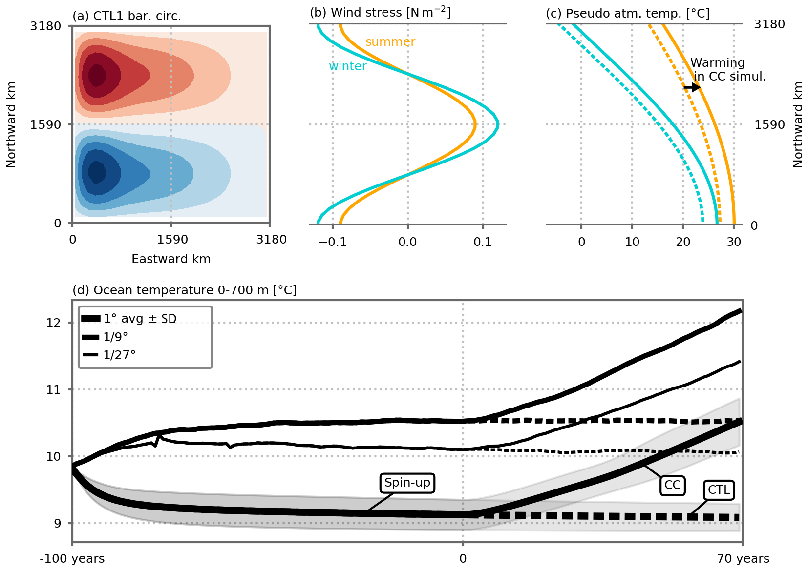
Figure 1(a) Barotropic circulation over the model domain (average of the five 1∘ resolution preindustrial control simulations; see also Fig. A2 for individual configurations) and analytical external forcings as a function of latitude: (b) wind stress (N m−2), and (c) pseudo-atmospheric temperature (∘C). The forcings vary seasonally in a sinusoidal manner between winter (blue) and summer (orange) extrema. In the climate change simulations, the pseudo-atmospheric temperature increases linearly in time between the dashed and solid lines (c). After 70 years of simulation, the linear atmospheric temperature increase reaches +2.8 ∘C. (d) Time series of annual ocean temperature (∘C) averaged between 0 and 700 m depth over the model domain. Years −100 to 0 correspond to the spin-up period under seasonal preindustrial forcing. The preindustrial control and climate change simulations (CTL and CC, respectively) discussed in this paper start at year 0. The 1∘ resolution time series shows the average of the five 1∘ configurations. Shading indicates ±1 standard deviation. See Fig. A1 for individual 1∘ model configurations. The small peaks in the time series of the ∘ resolution spin-up around years −80 and −60 are due to a problem during the chaining of the spin-up jobs (which were set by periods of 2 years). These errors did not influence the equilibrium states, and we decided not to rerun the spin-up simulations to save computational resources.
The model is run in a configuration adapted from previous studies (Krémeur et al., 2009; Lévy et al., 2012b; Resplandy et al., 2019). The domain geometry is a closed square basin on the β plane centered at ∼30∘ N, 3180 km wide and long and 4 km deep. The domain is bounded by vertical walls and by a flat bottom with a free slip boundary condition. The sea surface is kept free. The circulation is forced by analytical zonal distributions of wind stress, net heat flux and freshwater flux. The wind and buoyancy forcings are such that a double-gyre circulation is set up (Figs. 1 and A2). The wind stress is zonal and varies latitudinally in a sinusoidal manner between the extrema at the edges and the middle of the domain. The net heat flux takes the form of a restoration toward a zonal apparent air temperature profile. A portion of the net heat flux comes from solar radiation and is allowed to penetrate within the water column. A freshwater flux is also prescribed and varies zonally. It is determined such that, at each time step, the basin-integrated flux is zero.
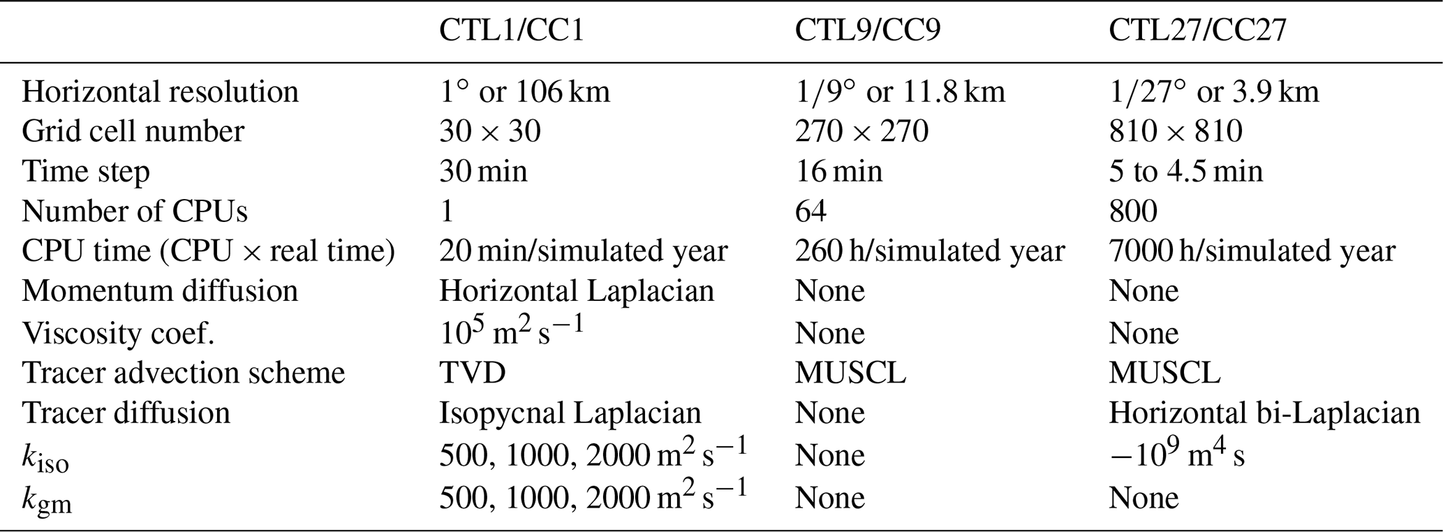
We use three horizontal resolutions: 106 km (1∘), 12 km (∘) and 4 km (∘). For each resolution, time steps, numerical schemes and isopycnal/horizontal diffusion are adapted (see Table 1). Note that diffusion is along the isopycnals only for the 1∘ coarse resolution. In the following, we will nevertheless use the term isopycnal diffusion regardless of the resolution for simplicity and because the diffusion is null or minimal at finer resolutions. On the vertical, 30 z levels are used whose thickness varies from 10 m at the surface to 500 m at depth. The upper 120 m contains 10 vertical levels; the upper 500 m contains 20 vertical levels. For the 1∘ resolution configurations, we used the Gent and McWilliams (1990, GM hereafter) eddy parameterization. This parameterization relies on two coefficients, an isopycnal diffusion coefficient (kiso) and a GM coefficient (kgm) that translates into a bolus velocity that acts to flatten isopycnals. For testing the sensitivity to the GM parameterization, we used five combinations of the isopycnal diffusion and GM coefficients: (1) 500 m2 s−1, (2) 1000 m2 s−1 and (3) 2000 m2 s−1 for both parameters and (4) 500 m2 s−1 and (5) 2000 m2 s−1 for the isopycnal diffusion parameter but keeping the GM coefficient at 1000 m2 s−1. We thus end up with seven different configurations: five eddy-parameterized at a coarse resolution (1∘) and two eddy-resolving at fine resolutions ( and ∘). In the following, results from the eddy-parameterized coarse-resolution configurations are synthesized by showing the average ±1 standard deviation across the five different configurations. Contrary to the ∘ configuration, the qualifier “eddy-permitting” is probably more appropriate for the ∘ configuration. Nevertheless to simplify and as the emphasis is put on the differences between the 1∘ resolution and the finer ones, we use the term eddy-resolving for both.
Table 1Resolution-dependent model features and parameters. For details on numerical schemes see Madec et al. (2017) and Lévy et al. (2001). Note that we added a minimum level of bi-Laplacian tracer diffusivity at ∘ to insure numerical stability, and this was not needed at the ∘ resolution. This bi-Laplacian diffusion acts on the horizontal unlike the Laplacian diffusion acting along isopycnals in the 1∘ resolution simulations.
The basin is initialized at rest with vertical profiles of temperature and salinity uniformly applied to the whole domain and homogeneous concentrations of the biogeochemical tracers. A 2000-year spin-up with an eddy-parameterized coarse-resolution configuration (1∘; m2 s−1) is then performed under preindustrial forcings (wind, air temperature and freshwater flux) varying seasonally in a sinusoidal manner between winter and summer extrema and repeated every year. Then, for each configuration, a climate change and a preindustrial control simulation are carried out from this initial coarse-resolution spin-up state in two steps (Figs. 1 and A1):
-
Step 1 comprises 100 years of spin-up under the same preindustrial control forcings, in order to reach an equilibrium for each configuration. These seven additional spin-ups (one for each configuration) are initialized with the annual mean coarse-resolution spin-up state. It is important to note that the final dynamical and biogeochemical equilibrium is different for each configuration (Figs. 1, 2, A1, A2, A4). The following section briefly describes these equilibrium and their differences.
-
Step 2 comprises a 70-year simulation for each configuration, following two scenarios. The preindustrial control scenario is the continuation of the spin-up; forcings are kept seasonal. In the climate change scenario, for air temperature, in addition to seasonal variations, we impose a linear trend of +0.04 ∘C yr−1 ( ∘C after 70 years). This trend roughly corresponds to the trend in surface air temperature of the simulations following the SSP5-8.5 scenario (Tokarska et al., 2020).
In total, 14 simulations of 70 years were run: seven configurations × two scenarios. In the following we will compare the differences between the eddy-resolving simulations ( and ∘ resolutions) and the mean of the eddy-parameterized simulations (1∘ resolution). A notable point is that after year 0, the residual drifts (CTL) are much smaller than the climate change trends (CC), which allows us to draw conclusions on the effect of the climate change forcing despite the fact that the spin-up is not yet fully achieved.
It is noteworthy that this experimental design implies that each climate change simulation starts from a different initial state. This strategy has the advantage that each initial state represents an equilibrated control state for the given set of resolution and parameter choices. For each simulation, the impact of climate change is evaluated as the difference between the climate change and preindustrial control simulations, and this difference depends on model choices but may also depend on the differences in the control simulations. Another option would have been to start the climate change simulations from the same initial conditions, but this would have had the consequences of a strong drift at the start of the eddy-resolving climate change simulations (as can be seen in the first 40 years of the spin-up, Fig. 1). Our choice is also consistent with the fact that shaping different equilibrium states is part of the role of the eddies. We can also note that none of the eddy-parameterized configurations that we explored has achieved an equilibrium state that comes close to the eddy-resolving configurations (Fig. A1).
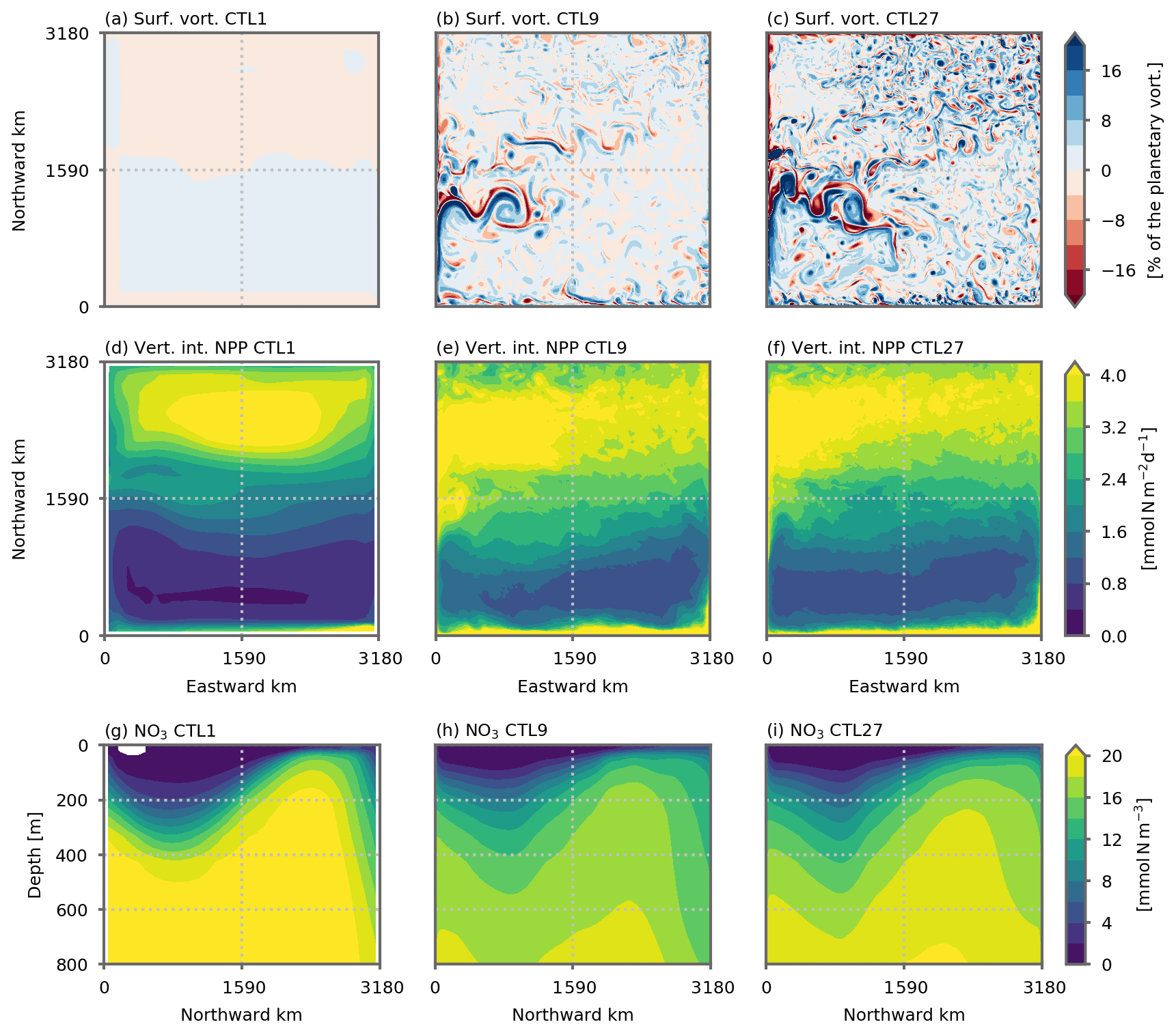
Figure 2(a, b, c) Surface relative vorticity (% of planetary vorticity), (d, e, f) vertically integrated net primary production (NPP, ) and (g, h, i) vertical distribution of nitrate (zonal mean, mmol N m−3) in the preindustrial control simulations at (a, d, g) 1∘, (b, e, h) ∘ and (c, f, i) ∘ resolution. Vorticity is computed with 2 d averaged velocity fields. NPP and nitrate distribution are averaged over the last 5 years of the simulations (years 66 to 70). The 1∘ resolution distribution is the mean of the five 1∘ configurations (see Figs. A4 and A2 for individual distributions).
2.2 Equilibrium states
As noted above, the dynamical and biogeochemical equilibrium states differ for each model configuration. These differences have been more extensively discussed in a similar setup in Lévy et al. (2010, 2012b) and Lévy and Martin (2013) and are briefly discussed in the following. It can be noted that the differences between the coarse-resolution equilibrium states on one hand and the fine-resolution equilibrium states on the other hand are much larger than the differences within the five (two) coarse-resolution (fine-resolution) spin-ups (Fig. 1).
The main features of the model's solution comprise a western boundary current separating an oligotrophic subtropical gyre in the south of the domain from a productive subpolar gyre in the north (Figs. 2 and A2). As resolution increases, mesoscale eddies and filamentary structures emerge in the relative surface vorticity field (Fig. 2a, b, c). In all simulations, the barotropic circulation is characterized by an anticyclonic circulation in the south and a cyclonic circulation in the north (Fig. A2). But as resolution increases, the non-linear effect become more important and small recirculation gyres appear close to the domain's northern and southern boundaries.
The divergence of the horizontal Ekman flux induces downwelling and a depressed nitracline in the subtropical gyre, as well as upwelling and a raised nitracline in the subpolar gyre (Figs. 2 and A4). The model's nitracline follows the thermocline very closely (Fig. A10). Nitrate supplies to the euphotic layer are seasonal and driven by the seasonal deepening of the mixed layer, which is strongest in the north of the domain (Fig. A9). This seasonal supply leads to an intense spring bloom in the subpolar gyre and to a weaker winter bloom in the subtropical gyre, where nitrate supplies are lower (Figs. 2 and A2). Over an annual average, this leads to a strong contrast between the subpolar gyre, where annual mean NPP is large, and the subtropical gyre characterized by low levels of annual mean NPP. We can also note that nitrate gradients in the thermocline are weaker at fine resolutions than at the coarse resolution (Fig. 2), in accordance with weaker stratification (Fig. A10). This is associated with lower sub-surface nitrate concentrations. We can note the opposed effect between and ∘ (Fig. 2) with a slightly larger sub-surface nitrate concentration at ∘ compared to ∘. These differences in equilibrated nitrate distribution lead to differences in equilibrated NPP between our different models runs (Fig. 2), but importantly the strong contrast between the two gyres is present is all simulations.
2.3 Nitrate budgets
In our simulation, NPP is constrained by nitrate supplies from the sub-surface into the sunlit surface layers where photosynthesis can occur. Nitrate budgets are thus used to investigate the processes driving changes in NPP. We focus our analysis on a predefined region within the model's subpolar gyre where the strongest NPP decline is observed (Figs. 2 and 3). This subpolar box is shown by the dashed horizontal black lines in Fig. 3; it is bounded by the change of sign in the wind stress curl forcing in the south and excludes the northern boundary. The local nitrate budget can be expressed as , where is the divergence of the advective fluxes, is the vertical diffusion term, L(N) is isopycnal diffusion, and S(N) represents the biological nitrate sources (regeneration) and sinks (NPP). u is the total velocity and includes the bolus velocity of the GM parameterization at the coarse resolution. Integrating this equation over the subpolar box and depth D leads to
The angle brackets stand for the horizontal integral over the subpolar box. The first term on the left hand side is the integral of the advective fluxes entering/exiting the subpolar box between the surface and depth D. It is obtained from the volume integral of the advective fluxes' divergence using Stoke's theorem. The subpolar box being closed at the east and west, it is computed as the sum of three nitrate advective fluxes: (1) the meridional flux entering through the southern boundary of the box between the surface and depth D, (2) the vertical flux entering at depth D, and (3) the meridional flux going out through the northern boundary of the box between the surface and depth D. Of interest here are the advective fluxes supplying nitrate and thus the fluxes entering the subpolar box, i.e., the vertical flux and the meridional flux through the southern boundary (Fig. A5). The total transport term shown in Fig. 4 represents these entering fluxes and contains the sum of the vertical flux and of the meridional flux at the southern boundary. It also contains isopycnal mixing, which is of second order (Fig. A5).
In the preindustrial control simulations, above ∼50 m depth, nitrate supplies to the subpolar box are dominated by vertical mixing, whereas deeper than ∼50 m they are dominated by the transport term (Fig. 4b). As resolution increases, this separation continues to hold although the respective intensities are modified: advective fluxes are stronger at the and ∘ resolutions than at the 1∘ resolution (Fig. 4c, d).
The separation between mean and eddy transport in this budget was achieved following the Reynolds averaging method. u and N are broken into a mean component ( and ) and a fluctuating eddy component (u′ and N′ with and ), leading to
The overbar is an averaging operator (in this study a spatio-temporal annual-mean averaging over boxes of 1∘) used to separate the mean from the fluctuating component over a temporal and/or spatial scale larger than the typical eddy scales. With this operator, we decomposed the total advection term into a mean part including advection by mean velocities () and an eddy part (), which we computed as the residual between total and mean advection.
This eddy–mean separation is by nature imperfect and leads to mean and eddy components that remain heterogeneous (Fig. A11) but is nevertheless useful to obtain an estimate of the contribution of each component. At a 1∘ resolution, the explicit (Reynolds) eddy term is close to zero and we estimated the parameterized eddy component as the sum between the two terms included in the GM parameterization: advection by the bolus velocity and isopycnal mixing (Figs. 4, A5 and A6).
Finally, the change in nitrate transport in response to global warming is due to changes in nitrate distribution as well as changes in circulation. In order to evaluate these two contributions, we computed offline diagnostics of nitrate advection, using velocities from the preindustrial control simulations (uCTL) and nitrate from the climate change simulations (NCC) or vice versa (uCC and NCTL). More precisely, we used the following decomposition of the change in nitrate advective fluxes, :
with
3.1 Sensitivity of the decline in net primary production to model resolution
After 70 years of forcing by a linear increase in atmospheric temperature (reaching +2.8 ∘C, similar in magnitude to the global temperature increase at the end of 21st century in the SSP5-8.5 scenario; Tokarska et al., 2020), NPP has declined in all model simulations (Fig. 3). The simulated declines are particularly strong in the model's subpolar gyre, a region with elevated initial levels of NPP (Fig. 2) and where we will now focus the analysis. The integrated NPP over the model's subpolar box decreases by , −0.51 and −0.44 in our three model resolution versions, representing %, −14 % and −12 %, with the horizontal resolution set at 1, and ∘, respectively (Fig. 3). Thus the NPP declines differ markedly between each other depending on the resolution, with the decline in NPP halved at the finest resolution compared with the decline projected at the coarse resolution. Locally, the intensity of the decline in the coarse-resolution model's versions exceeds −1.5 . The intensity and distribution of these local changes slightly vary among the five coarse-resolution configurations. But with a finer grid resolution, they are strongly reduced (Fig. 3).
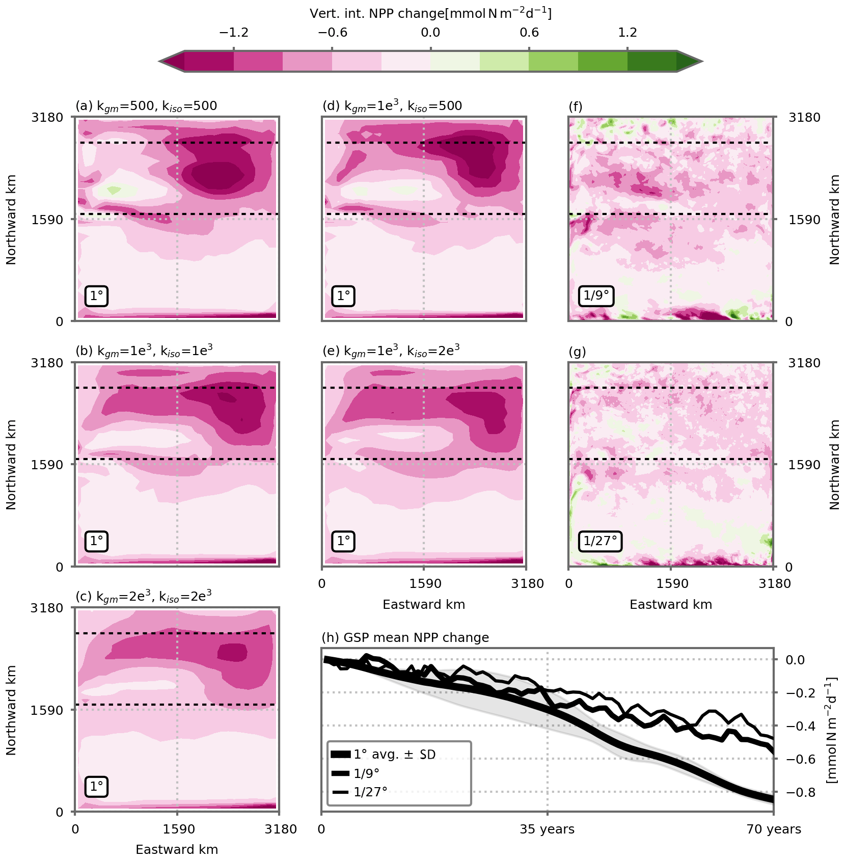
Figure 3Projected decrease in net primary production (NPP, ) under a high-emission scenario in (a, b, c, d, e) five 1∘, (f) one ∘ and (g) one ∘ model simulations. The NPP change is vertically integrated over the entire water column and taken as the difference between the last 5 years of the climate change and preindustrial control simulations (years 66 to 70). The dashed horizontal black lines delineate the model's subpolar box over which diagnostics for (h) and Figs. 4, 5, 6 and 7 are performed. This is where simulated NPP is strongest (Fig. 2) and where the simulated NPP decline is also strongest. (h) Time evolution of the NPP decrease in the model's subpolar box in response to climate change, for the three model resolutions. The decrease is computed relative to the preindustrial control simulations. The 1∘ resolution time series shows the average of the five 1∘ configurations. Shading indicates ±1 inter-model standard deviation. See Fig. A1 for individual model simulations.
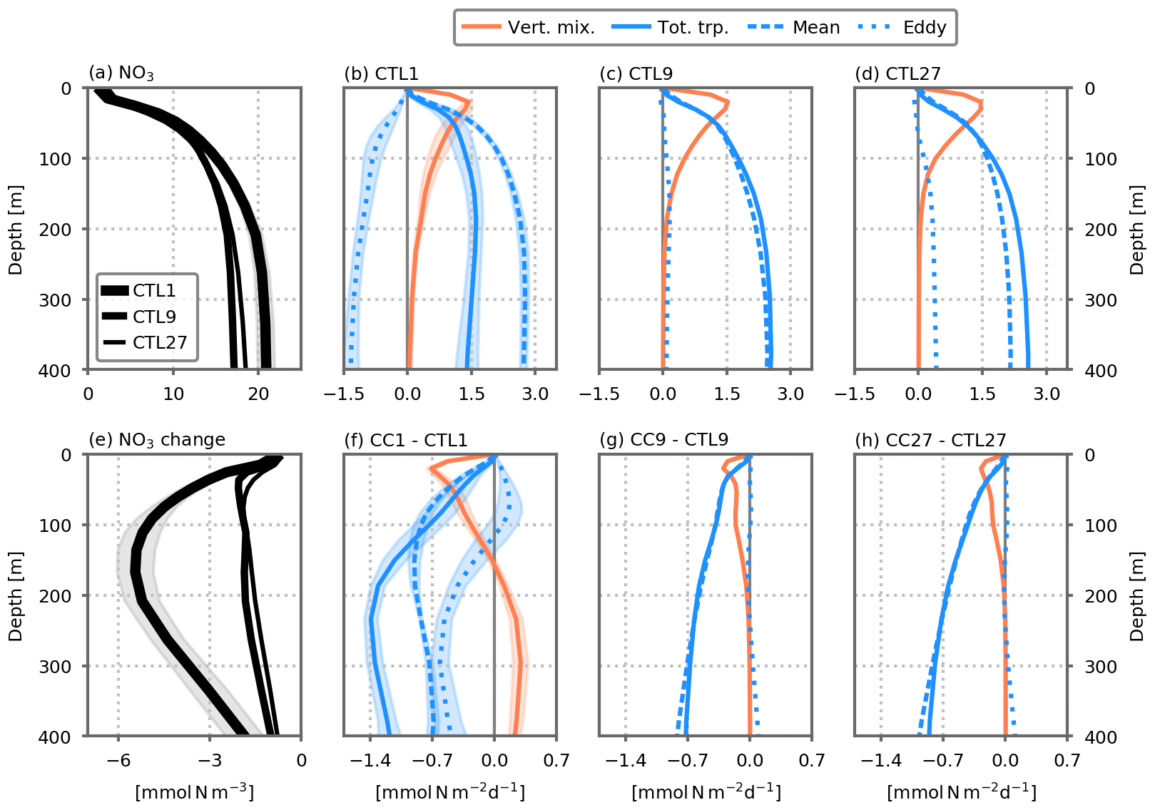
Figure 4 Nitrate concentrations (mmol N m−3) and nitrate supplies () averaged over the model's subpolar box (dashed horizontal black lines in Fig. 3). (a) Nitrate profiles in the preindustrial control simulations, for the three resolutions. (b, c, d) Dynamical nitrate supplies, cumulated between the surface and depth D in the preindustrial control simulations, against D. (e, f, g, h) Changes in these profiles between the climate change and preindustrial control simulations. In the coarse-resolution simulations (CTL1/CC1), the profiles show the average of the five 1∘ configurations. Shading indicates ±1 standard deviation. The total transport term (solid blue line) comprises the sum of vertical advection across depth D and meridional advection through the southern border of the model's subpolar box; in the case of the 1∘ simulations, total transport also includes eddy parameterizations (including advection by bolus velocity and isopycnal mixing). Total transport is the sum of mean and eddy transport. In the fine-resolution simulations (CTL9/CC9, CTL27/CC27), the mean and eddy transport terms are derived from Reynolds decomposition (see the Methodology section). In the coarse-resolution simulations (CTL1/CC1), the mean transport represents the resolved transport by the coarse-resolution velocity field, and the eddy transport includes the two eddy parameterization terms. See also Figs. A5 and A6 for individual fluxes. All profiles are averaged over years 66 to 70.
3.2 Decline in nutrient supply pathways
The decline in NPP in the model's subpolar box stems from the decline in the supply of nutrients supporting phytoplankton growth, which is associated with the decline in nitrate concentrations in the thermocline (Figs. 4a, e and A4). About half of the NPP decrease results from a decline in NPP supported by newly supplied nutrients, which are mainly in the form of nitrate, with the remaining half arising from decreased NPP supported by locally regenerated nutrients (mostly in the form of ammonium, Fig. A3). The mean f ratio on the subpolar box is about 0.43 all along the simulations (Fig. A3, fourth column) albeit with a very small decline (from ∼0.43 to ∼0.40) in the climate change simulations. This slight decline is consistent with the lower primary production regime having a lower f ratio (Sarmiento and Gruber, 2006, p. 166). We should also note that changes in the f ratio in response to warming might be underestimated here because the direct impact of increasing temperature on biological rates, which has been shown to affect the response of biology to climate change (Olonscheck et al., 2013; Lewandowska et al., 2014; Laufkötter et al., 2015), is not accounted for in this study.
A closer examination of nitrate trends within the model's subpolar box provides insights into the physical mechanisms controlling the declining nitrate concentrations in the thermocline in our coarse-resolution simulations (Fig. 4). The traditional paradigm (Steinacher et al., 2010; Fu et al., 2016; Bindoff et al., 2019; Kwiatkowski et al., 2020) for the decrease in NPP is confirmed. Indeed in the euphotic layer (top 150 m), there is a strong reduction in nutrient supply by vertical mixing (Fig. 4f, orange line). This decrease is associated with increasing stratification (Fig. A10). However, similarly to what has been shown for the North Atlantic in coarse-resolution ESM projections (Whitt, 2019; Whitt and Jansen, 2020; Tagklis et al., 2020), the decrease in nutrient supply is also controlled by the sub-surface nutrient reservoir and the fluxes fueling it. Nitrate concentrations in the top 400 m strongly decrease under our global warming scenario (Fig. 4e) because of a reduction in nutrient advection. Under global warming, the net advective supply of nitrate in the sub-surface (between 100 and 400 m) is strongly reduced (Fig. 4f, blue line; see also each component of the advective flux in Fig. A6).
As the resolution increases from 1 to and ∘, the mechanisms described previously still hold. However, despite similar mean states for the three resolutions at equilibrium (preindustrial control simulations; Fig. 4b, c, d), the climate-change-induced decline in vertical mixing to the euphotic layer and in sub-surface advection are both dampened when resolution increases (Fig. 4f, g, h). At the coarse resolution (1∘), vertical mixing decreases by 48±4 %, whereas it only decreases by 18±1 % in the finer-resolution models (Fig. 7). Likewise, nutrient advection decreases by 83±5 % at the coarse resolution compared to only 27±2 % at the finer resolutions. A large part of the attenuation occurs when the resolution is changed from 1 to ∘, but the attenuation is much more moderate between and ∘. This is consistent with the expectation that resolution of mesoscale dynamics should be nearly achieved at ∘ in the latitudinal range considered here but not fully (see also Figs. 1 and A1). Moreover, we expect further differences to emerge with grids finer than ∘ which would allow resolving sub-mesoscale dynamics (Lévy et al., 2010; Gula et al., 2016; McWilliams, 2016; Uchida et al., 2019).
3.3 On the role of local eddy processes
A legitimate question is whether the differences between our coarse-resolution and fine-resolution models are due to local small-scale eddy processes not adequately captured by the eddy parameterization or to different responses of the mean large-scale state to global warming. To address this question, we separated the mean and eddy transport of nitrate, in the two eddy-resolving simulations following Lévy and Martin (2013), with a spatio-temporal annual-mean averaging over boxes of 1∘. In the coarse-resolution simulations, eddy transport is parameterized by a bolus advection term (Gent and McWilliams, 1990) and isopycnal mixing.
This analysis reveals the dominant role of the mean advection in fueling the sub-surface nitrate reservoir at equilibrium in the two eddy-resolving models (preindustrial control simulations; dashed blue lines in Fig. 4c, d). Eddy advection supplies a minor addition of nutrients in the subpolar box (mostly at ∘), essentially through the eddy meridional advection (Fig. A5). In the eddy-parameterized models, the eddy parameterization strongly opposes the resolved transport, removing nutrients from the surface of the subpolar box mainly through the vertical bolus advection term (Figs. 4b and A5).
In the eddy-resolving climate change simulations, most of the decline in nutrient input is explained by a reduction in mean nitrate transport (Fig. 4g, h). In the eddy-parameterized simulations, the eddy component plays a larger role and explains approximately one-third of the total transport decrease at 200 m (Fig. 4). As for the preindustrial control simulation, it is dominated by changes in the vertical bolus advection term (Fig. A6).
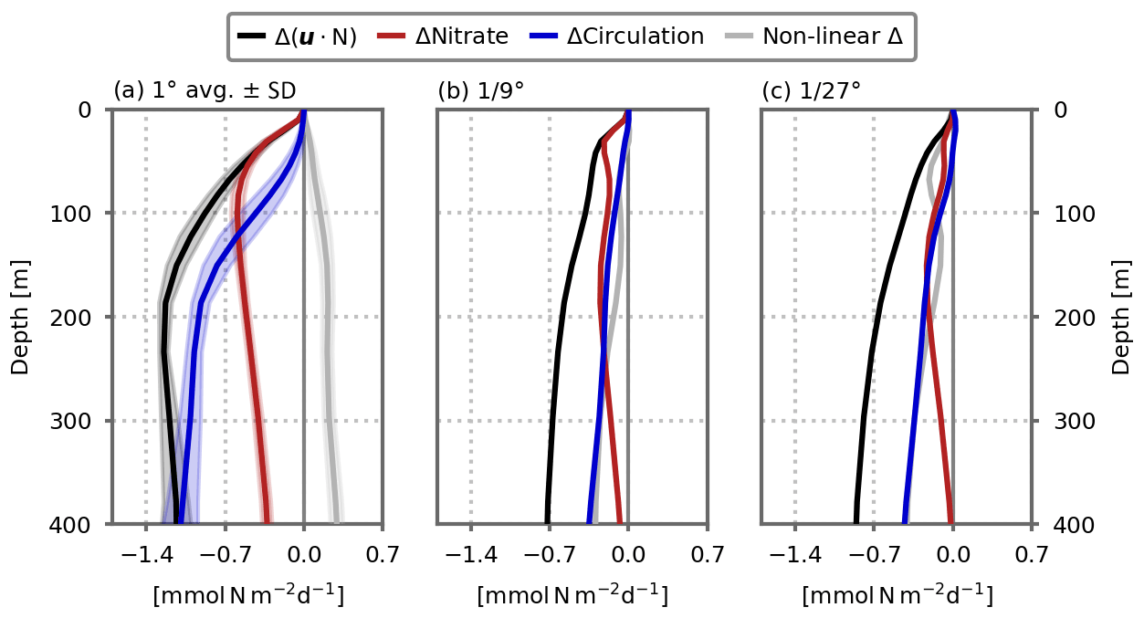
Figure 5Role of circulation change versus nitrate distribution change in explaining the decline in the nitrate advection flux () in response to global warming in the model's subpolar box, cumulated between the surface and depth D, for the (a) 1∘, (b) ∘ and (c) ∘ resolution configurations. The black lines show the simulated change, which is decomposed into three components: the red lines show the component related to the change in nitrate distribution; the blue lines show the component related to the change in circulation; the gray lines show the residual due to non-linear changes. See Eqs. (3) to (6) for details. In (a), the profiles show the average of the five 1∘ configurations. Shading indicates ±1 standard deviation.
3.4 On the role of circulation changes
Another question is how changes in nitrate transport (black lines in Fig. 5) are related to changes in circulation. To examine this question, we first computed in offline mode the advective transport of nitrate keeping the nitrate distribution fixed to its preindustrial state. By doing so, we accounted only for changes in circulation and neglected changes in nitrate distribution (blue lines in Fig. 5). In a similar manner, we kept the circulation constant and accounted only for the changes in nitrate distribution (red lines in Fig. 5). Due to non-linearities, the sum of circulation-induced (blue lines) and nitrate-induced (red lines) changes is not equal to the total change (black lines) and a residual remains (gray lines in Fig. 5).
In the euphotic layer (upper 0–100 m), the change in nitrate transport is mostly attributable to a change in nitrate concentrations, at all resolutions. But deeper in the water column, the situation is reversed and the change in circulation is responsible for most of the change. In fact at 400 m depth, the change in nitrate transport is largely explained by circulation changes in all of our simulations. This result highlights the crucial role of circulation changes, which directly affect the resupply of the sub-surface nitrate reservoir (between 100–400 m), with the consequence of affecting the mean nitrate gradients, particularly in the upper layers (0–100 m, Fig. 4e) and thus the nitrate fluxes closer to the surface. We can note a stronger contribution of non-linearities in this simple analysis as the model resolution increases.
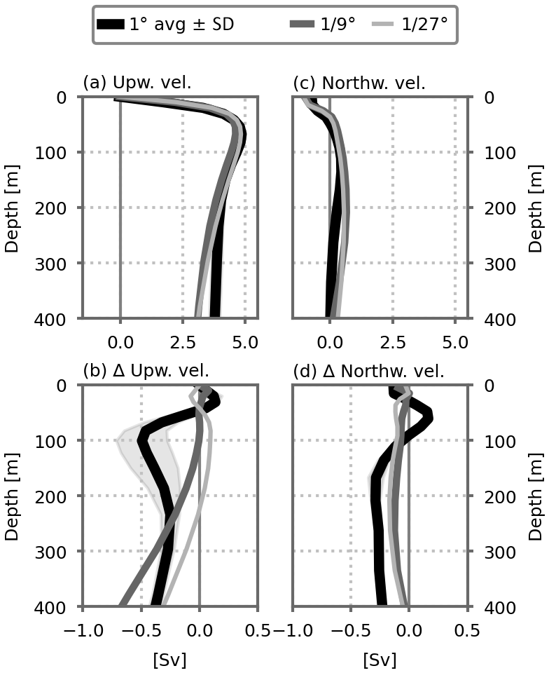
Figure 6Vertical profiles of (a) the northward and (c) upward water transport (in Sv) entering the model's subpolar box (dashed horizontal black lines in Fig. 3) in the preindustrial control simulations for each resolution. (b, d) Changes in these profiles between the climate change and preindustrial control simulations. The thick black lines show the average of the five 1∘ configurations. Shading indicates ±1 standard deviation.
To further link our results to circulation changes, we then examined how the water transport through the subpolar box was modified in our climate change simulations (Fig. 6). In our model, the main transport pathway to the subpolar box originates from upwelling and from northward advection at the sub-surface (between 50 and 400 m) (Fig. 6a, c). With warming, these upward and sub-surface northward transports both decline (Fig. 6b, d). The mean transports are similar in the equilibrium states between the coarse- and fine-resolution simulations, but they respond differently to warming. At the coarse resolution, the decline in the upward transport is particularly strong, −0.5 Sv at ∼100 m depth (Fig. 6b). This is in phase with the strong decline in nitrate vertical advection at a similar depth discussed above (blue lines in Fig. A6). At finer resolutions, the decline in the vertical flow is close to zero at ∼100 m, but it increases with depth, reaching an amplitude similar to the coarse-resolution simulations at ∼400 m, Sv. In the finer-resolution simulations, the sub-surface northward flow decline is also weaker, Sv against Sv at the coarse resolution below 100 m depth (Fig. 6d).
Previous coarse-resolution modeling studies (Whitt, 2019; Whitt and Jansen, 2020; Tagklis et al., 2020) have suggested that the climate-change-driven decline in North Atlantic NPP is strongly linked to changes in the Meridional Overturning Circulation (MOC). This link presumes that the slowdown in the upper branch of the MOC is associated with a decrease in the strength of the portion of the Gulf Stream that conveys nutrients northward (Whitt, 2019). In our simplified model configuration, the MOC (here diagnosed by the meridional stream function in the z coordinate, Fig. A8) transports waters from the subtropical gyre to the north at a depth between ∼100 and ∼400 m: 1.75±0.16 Sv at the 1∘ resolution, 3.14 Sv at ∘ and 2.94 Sv at ∘ (flow through the vertical black lines in Fig. A8). Once these waters reach the northern boundary of the domain, they are entrained downward by convection to depths of 1000 m and more (Fig. A9) before they return southward toward the southern boundary where they are upwelled back to the surface. In our coarse-resolution simulations, this overturning cell is strongly slowed down under global warming, inducing in particular a strong reduction, Sv ( %), in the water transport between the two gyres (Fig. A8). The slowing of the overturning circulation is associated with a decrease in the maximum depth of the mixed layer (MLD) in the northern part of the domain where convection occurs (Fig. A9). The maximum MLD shoals from over 2000 to ∼300 m after 70 years of climate change forcing (e.g., Fig. A9c). At finer resolutions, the MOC is also slowed down, but this slowdown is less pronounced (Fig. A8). The flow between 100 and 400 m between the two gyres is reduced by −0.58 and −0.85 Sv (−18 % and −29 %) at and ∘ resolution, respectively. It is also exemplified by the maximum depth of the mixed layer in the northern part of the domain which shoals less than it does at the coarse resolution, from ∼1000 to ∼700 m (Fig. A9r, u).
The different responses of the MOC between our coarse- and fine-resolution simulations can be partly related to the differences in stratification in the north of the domain. The fine-resolution equilibrium states are initially less stratified than the coarse-resolution ones (Fig. A10, first column). As a consequence, surface heating during the transient climate warming for the fine-resolution simulations penetrates deeper into the interior and leads to a weaker increase in stratification (Fig. A10, last column) and thus a weaker decrease in convection and in meridional circulation.
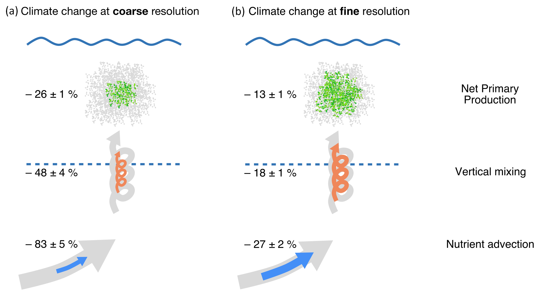
Figure 7Schematic representation of the projected response of net primary production (NPP) and of the nutrient fluxes (advection and vertical mixing) supporting it to warming, with our (a) eddy-parameterized coarse-resolution (1∘) and (b) eddy-resolving fine-resolution (, ∘) simulations, in the model's subpolar gyre. Decline in nutrient advection is assessed from changes between the surface and 200 m depth (Tot. trp. in Fig. 4). Decline in vertical mixing is evaluated at 25 m depth, which is where the decrease is maximal. NPP change is vertically integrated over the entire water column. Changes at the coarse resolution are the average of the five 1∘ configurations ±1 standard deviation. Changes at the fine resolutions are the average of the and ∘ configurations ± half of the difference between the two. The background diagrams in gray represent the initial control situation, while the colored diagrams represent the situation after 70 years of warming.
Based on a wind- and buoyancy-driven double-gyre model configuration with an idealistic scenario of global warming, we have shown that the projected decline in NPP is strongly sensitive to horizontal grid resolution, with a decline which is halved at an eddy resolution: % versus % at the coarse resolution (Fig. 7). Moreover, we have also found that this sensitivity is much stronger than the sensitivity to a large set of eddy parameterization coefficients (kiso and kgm). This result is due to the much weaker decline in nutrient transport at fine resolutions, % versus % at the coarse resolution, combined with a weaker decrease in vertical mixing, % vs. % (Fig. 7).
A key result of our study is that the resolution-related uncertainties in the NPP projections stem from the high sensitivity of mean ocean transport projections to resolution. This sensitivity is currently being debated. Regarding the Atlantic MOC (AMOC), some studies show a weaker decline as resolution increases (Roberts et al., 2004; Delworth et al., 2012; as with our model MOC), whereas other studies show an amplified response (Weijer et al., 2012; Spence et al., 2013; Jackson et al., 2020; Roberts et al., 2020). It has been suggested that the intensity of the AMOC decline may be related to its intensity in the control climate: the stronger the initial AMOC, the stronger the decline (Gregory et al., 2005; Winton et al., 2014; Jackson et al., 2020; Roberts et al., 2020). The opposite is found here: at fine resolutions, the model's MOC is stronger in the control climate but the response is dampened in the global warming scenario. The AMOC intensity in the control climate itself has been shown to be sensitive to resolution but with no consensus yet on the sign of this sensitivity (Winton et al., 2014; Hirschi et al., 2020). The reason for the sensitivity of control and projected AMOC to resolution remains unclear and differs between studies. The potential causes mentioned are stronger air–sea interactions at fine resolution (Hirschi et al., 2020), different spatial distributions of perturbations by the eddies (Spence et al., 2013) or the introduction of biases (Delworth et al., 2012).
Another possible reason for the high sensitivity to resolution of projected ocean circulation changes could be derived from the “eddy saturation” and “eddy compensation” phenomena which are actively studied in the Southern Ocean (Farneti et al., 2010; Farneti and Delworth, 2010; Meredith et al., 2012; Munday et al., 2013; Mak et al., 2017). They stand for the low sensitivity of stratification and overturning circulation, respectively, to an increase in wind forcing in eddy-resolving models. The connection between the two phenomena is subject to ongoing research (Meredith et al., 2012). Eddy saturation results from the balance between the steepening of the isopycnal by the wind stress and the flattening by eddies (Mak et al., 2017). One could imagine that similar competing processes are at work in our eddy-resolving simulations of climate change, warming stratifying the ocean versus eddies destratifying it. One clue in that direction is that, as in Munday et al. (2013), surface eddy kinetic energy increases with global warming in the eddy-resolving simulations. Eddy saturation is poorly represented by the GM parameterization (Farneti et al., 2010; Munday et al., 2013, 2014); however simple modification of this parameterization can lead to the emergence of the phenomenon (Mak et al., 2017).
The GM parameterization has improved the representation of circulation in ocean models (Gent and McWilliams, 1990), but its ability to fully represent the impact of eddies is still questioned (Eden and Greatbatch, 2008; Marshall et al., 2012; Zanna et al., 2017; Mak et al., 2017). The parameterization represents a net sink of energy as the potential energy extracted from the iso-neutral slopes is lost. Moreover, even coupled with Laplacian viscosities, it neglects the eddy effects on the momentum equation, the so-called eddy Reynolds stresses (Marshall et al., 2012; Zanna et al., 2017; Mak et al., 2018). These deficiencies in the representation of the eddies have consequences for the mean flows and the transport of tracers (Li et al., 2016; Tamarin et al., 2016; Zanna et al., 2017; Klocker, 2018). In our simulations, the mean equilibrium state in the eddy-parameterized simulations deviates from the eddy-resolving ones, with little sensitivity to the choice of the GM and isopycnal diffusion coefficients. And importantly, the global-warming-driven changes in circulation and the subsequent NPP decline greatly differ from the simulated changes in the eddy-resolving simulations (Fig. 7). This suggests that strong biases in global warming NPP projections could come from inadequate eddy parameterizations. On a positive note, most of the biases stem from differences in the response of the mean flow to warming, which suggests that a better representations of the eddy impact on the mean flow may correct for it. Ongoing activities in that direction open optimistic perspectives (Marshall et al., 2012; Zanna et al., 2017; Mak et al., 2018).
The difficulty of attributing recently observed changes in NPP to climate change and even of detecting long-term trends (Wernand et al., 2013; Beaulieu et al., 2013; Boyce et al., 2010; Henson et al., 2016) make ESMs essential for anticipating anthropogenic changes in NPP. In this regard, it is key to understand the origins and consequences of ESM biases and/or projection uncertainties. One such bias, identified here, is the high sensitivity of NPP projections to model resolution. It is questionable how the bias highlighted here in an idealized regional setting can be extrapolated to global ESMs. The oceanic regime closest to our configurations is found in the North Atlantic. Our model captures important characteristics of the North Atlantic NPP system, in particular the reduction in NPP in response to global warming (Kwiatkowski et al., 2020) as well as the leading role of the nutrient advection in refueling nutrients at the sub-surface in the productive subpolar region (Williams et al., 2011). With our simplified model, we were able to investigate the consequences of a decline in the MOC driven by changes in air–sea heat fluxes and associated with the reduction in deep water formation of a unique water mass. However, changes in the AMOC may also be driven by freshwater input (Bras et al., 2021), driven by changes in wind stress pattern (Polovina et al., 2008; Yang et al., 2020), or related to changes in adjacent regions and involving the formation of different water masses (Delworth and Zeng, 2008; Bronselaer et al., 2016; Lique and Thomas, 2018; Bras et al., 2021). Moreover, the link between the reduction in deep water formation at high latitudes in the North Atlantic and the slowing of the AMOC may be more tenuous than previously thought (Lozier, 2012). Investigation of these different aspects would require more realistic configurations and more complex climate change scenarios. Global ESMs and CMIP6 framework scenarios incorporate such additional features, as well as the temperature sensitivity of biological processes that has been revealed to also affect the global-warming-driven response of biology (Olonscheck et al., 2013; Lewandowska et al., 2014; Laufkötter et al., 2015). All these elements are likely to further influence the sensitivity of NPP projections to model resolution.
Constraining uncertainties in ESM NPP projections is crucial because these projections are essential to assess the future evolution of marine biomass and the potential implications for fish catch potential and food security (Lotze et al., 2019). Although being only one piece of a much broader and more complicated response of the ocean to climate change, our results suggest that the uncertainty in NPP decline intensity under global warming may have been underestimated in recent policy-relevant reports such as IPCC (2019) and IPBES (2019). A natural next step to better assist in political decision-making is now to conduct climate change simulation with ESMs better representing oceanic eddies. Two conceivable strategies to conduct such simulations have already been explored for ocean dynamics: simulations with ESMs at finer ocean resolutions (Haarsma et al., 2016; Gutjahr et al., 2019; Roberts et al., 2004; van Westen and Dijkstra, 2021) and simulations with ESMs using improved eddy parameterizations (Zanna et al., 2017; Mak et al., 2018). Our study calls for pursuing research in that direction. Work is in progress to examine the sensitivity of carbon fluxes to eddy resolution. Such advances would be significant for the representation of the global carbon cycle and consequently for climate projections.
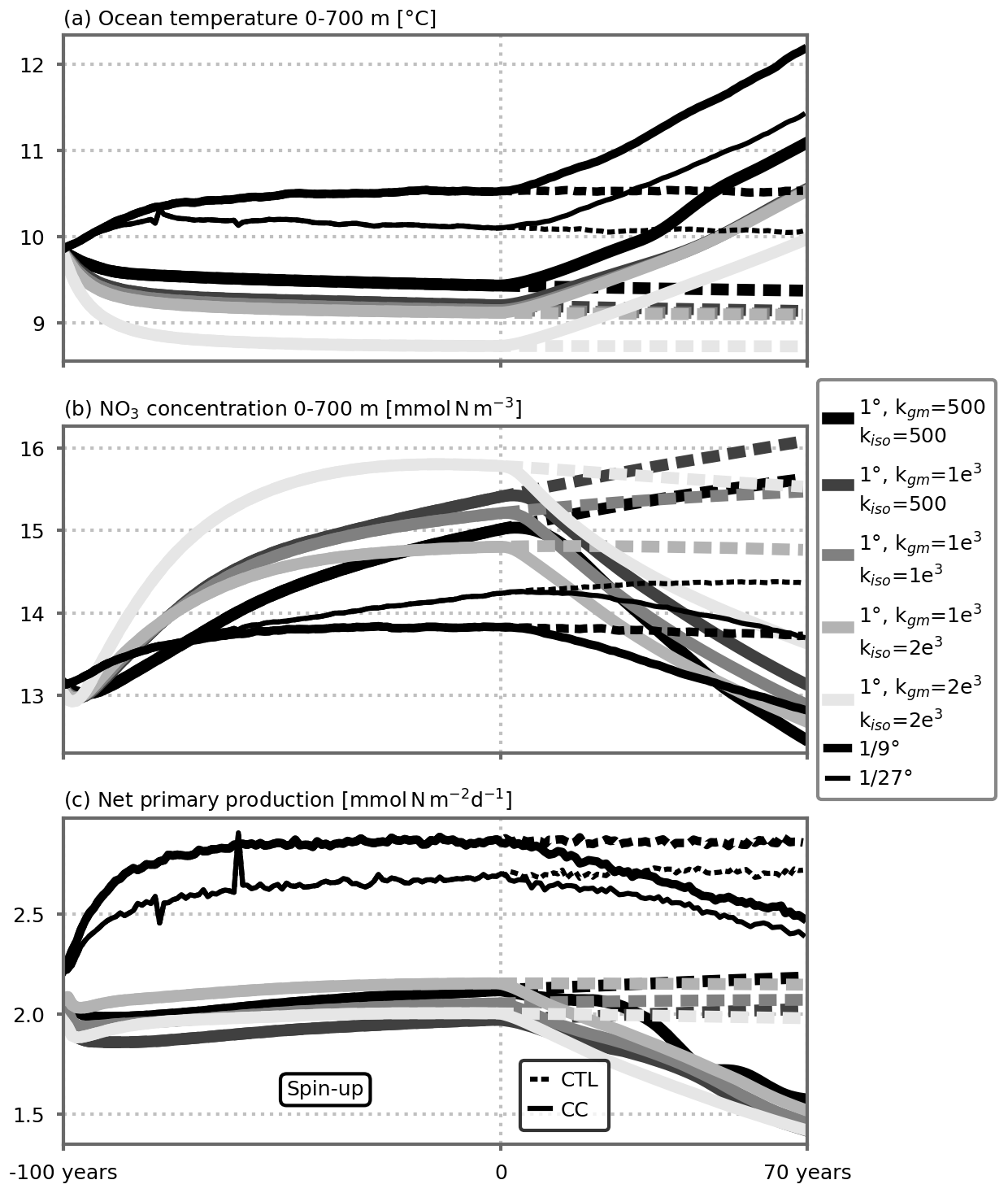
Figure A1Time series of (a) annual ocean temperature (∘C) and (b) annual nitrate concentration (mmol N m−3) averaged between 0 and 700 m depth and (c) vertically integrated net primary production (). All variables are averaged over the whole domain. Years −100 to 0 correspond to the spin-up period under seasonal preindustrial forcing. The preindustrial control and climate change simulations discussed in this paper start at year 0. Line thickness stands for the different resolutions, and the various shades of gray stand for the various eddy parameterizations. The small peaks in the time series of the ∘ resolution spin-up around years −80 and −60 are due to a problem during the chaining of the spin-up jobs (which were set by periods of 10 years). These errors did not influence the equilibrium states, and we decided not to rerun the spin-up simulations to save computational resources.
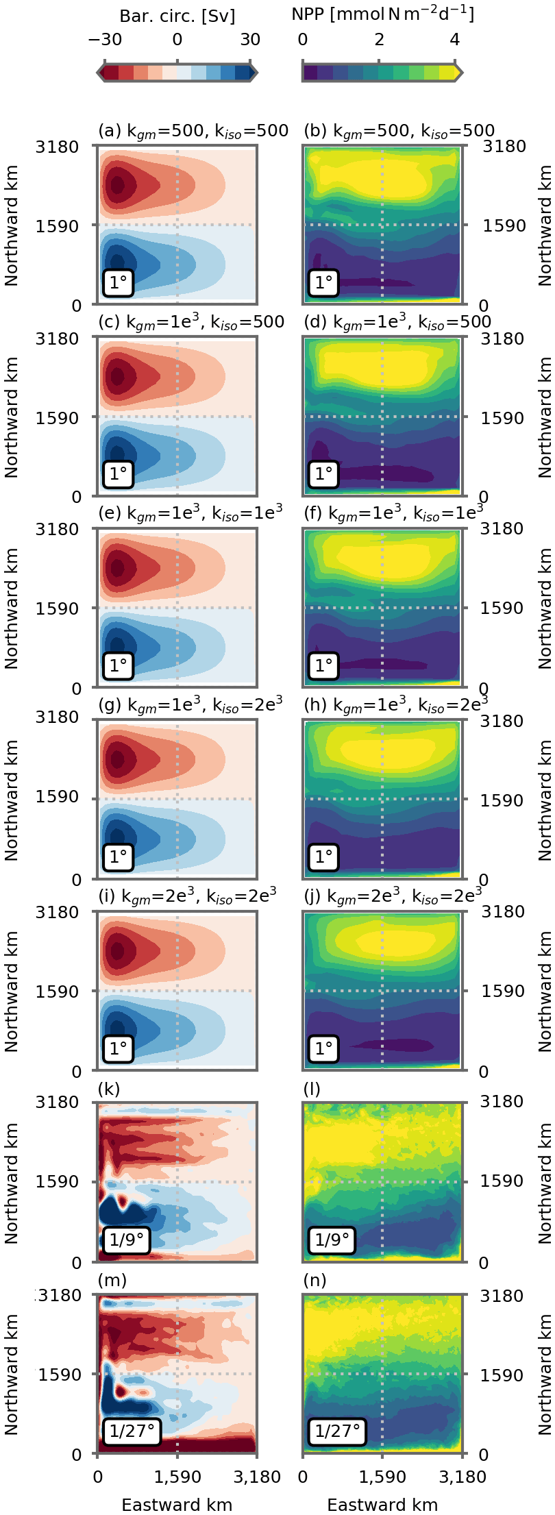
Figure A2The left column shows barotropic circulation (Sv), and the right column shows vertically integrated net primary production (NPP, ) in preindustrial control simulations. Panels (a)–(j) show the five 1∘ resolution configurations, and (k)–(n) show the and ∘ resolution configurations. All figures show the average over the last 5 years of the simulations (years 66 to 70).
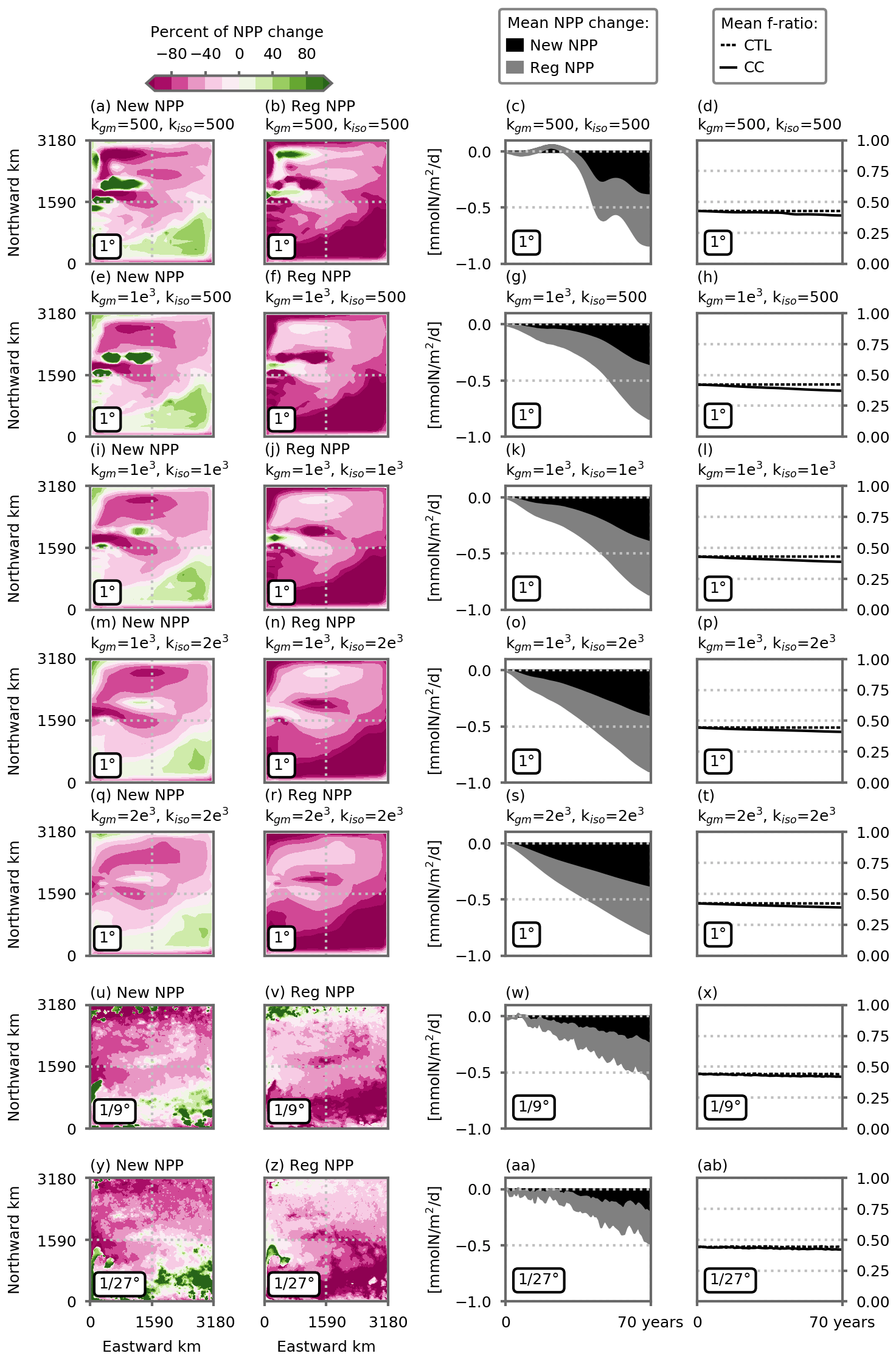
Figure A3Percentage of local change in vertically integrated net primary production (NPP) due to a change in new NPP (New NPP, first column) and regenerated NPP (Reg NPP, second column). Respective share of the NPP decrease from new NPP (black) and regenerated NPP (gray), averaged over the subpolar box (third column, ). Evolution of the f ratio averaged over the subpolar box in the preindustrial control and climate change simulations (fourth column, dashed and solid lines, respectively). Vertical integration up to 100 m depth where most of the NPP occurs. New NPP is the NPP supported by nitrate minus nitrification, and regenerated NPP is NPP supported by ammonium plus nitrification. The nitrification is handled in this way so that locally produced nitrate is counted as a source of regenerated production and not as a source of new production. The f ratio is computed as the ratio between new NPP and total NPP. Panels (a)–(t) show the five 1∘ resolution configurations, and (u)–(ab) show the and ∘ resolution configurations. The first two columns show the average over the last 5 years of the simulations (years 66 to 70).

Figure A4Vertical distribution of nitrate across the domain (zonal mean, mmol N m−3) in the preindustrial control simulations (first column) and the climate change simulations (second column) and the difference between the two (third column). Panels (a)–(o) show the five 1∘ resolution configurations, and (p)–(u) show the and ∘ resolution configurations. All figures show the average over the last 5 years of the simulations (years 66 to 70).
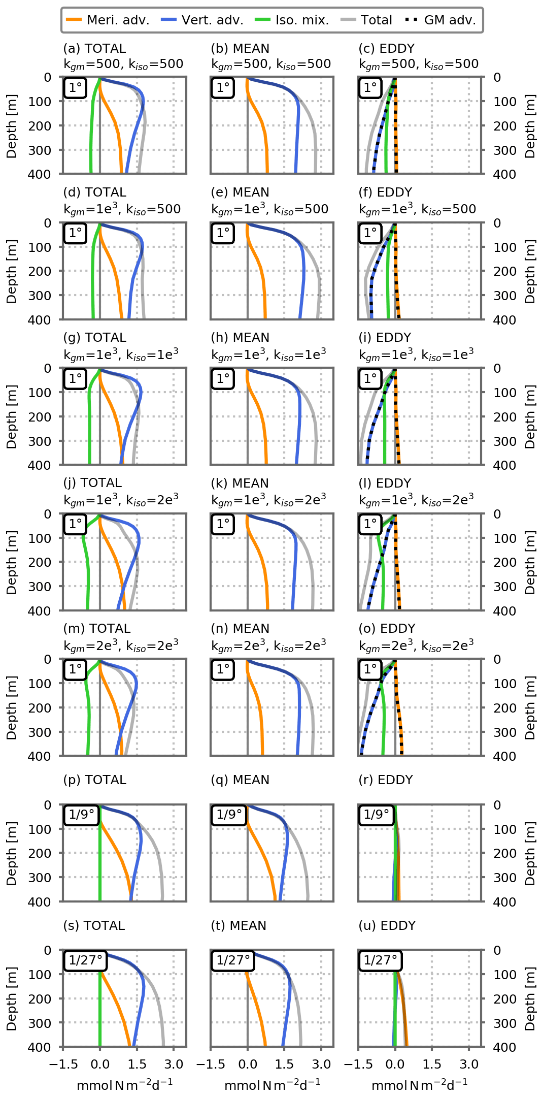
Figure A5Vertical profiles of dynamical nitrate supplies () in the model's subpolar box (dashed black lines in Fig. 3), cumulated between the surface and depth D in the preindustrial control simulations, against D. Total transport (gray lines here, solid blue lines in Fig. 4) is decomposed into three components: in orange, the meridional advective flux at the southern border; in blue, the vertical advective flux at depth D; and, in green, the isopycnal mixing. For each resolution, the total advective fluxes (first column) are broken into mean and eddy transport terms (the second and third columns, respectively). In the fine-resolution simulations (, ∘), they are derived from Reynolds decomposition (see the Methodology section). In the coarse-resolution simulations (CTL1/CC1), the mean transport represents the resolved transport by the coarse-resolution velocity field, and the eddy transport includes the two eddy parameterizations. Panels (a)–(o) show the five 1∘ resolution configurations, and (p)–(u) show the and ∘ resolution configurations. All figures show the average over the last 5 years of the simulations (years 66 to 70). Positive values indicate an inflow into the subpolar box.
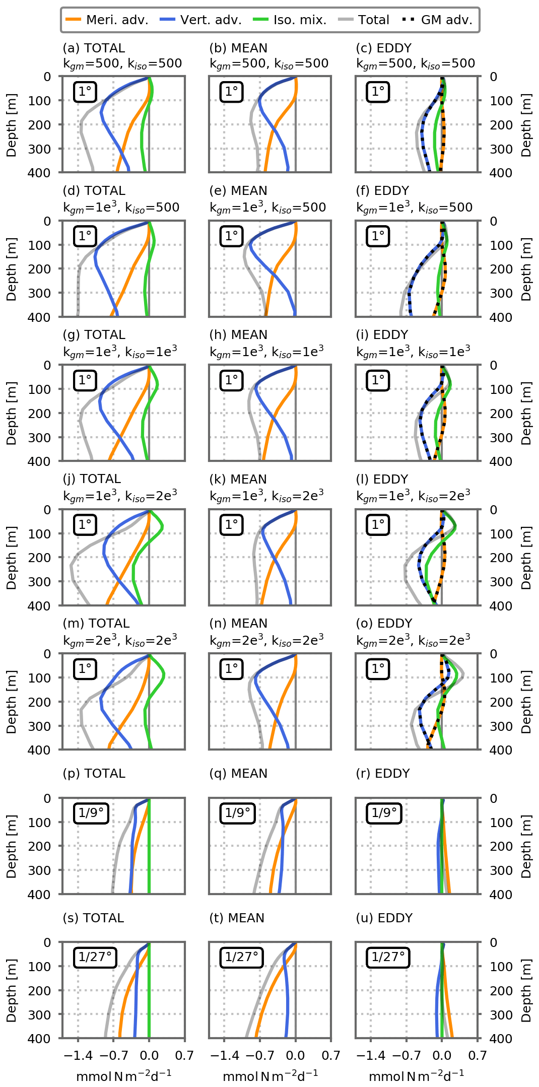
Figure A6Changes in the dynamical nitrate supplies () between the climate change and preindustrial control simulations. See Fig. A5 for details. The change is relative to the preindustrial control simulations. Positive values indicate an increase in nitrate input either because an inflow increases or because an outflow decreases.
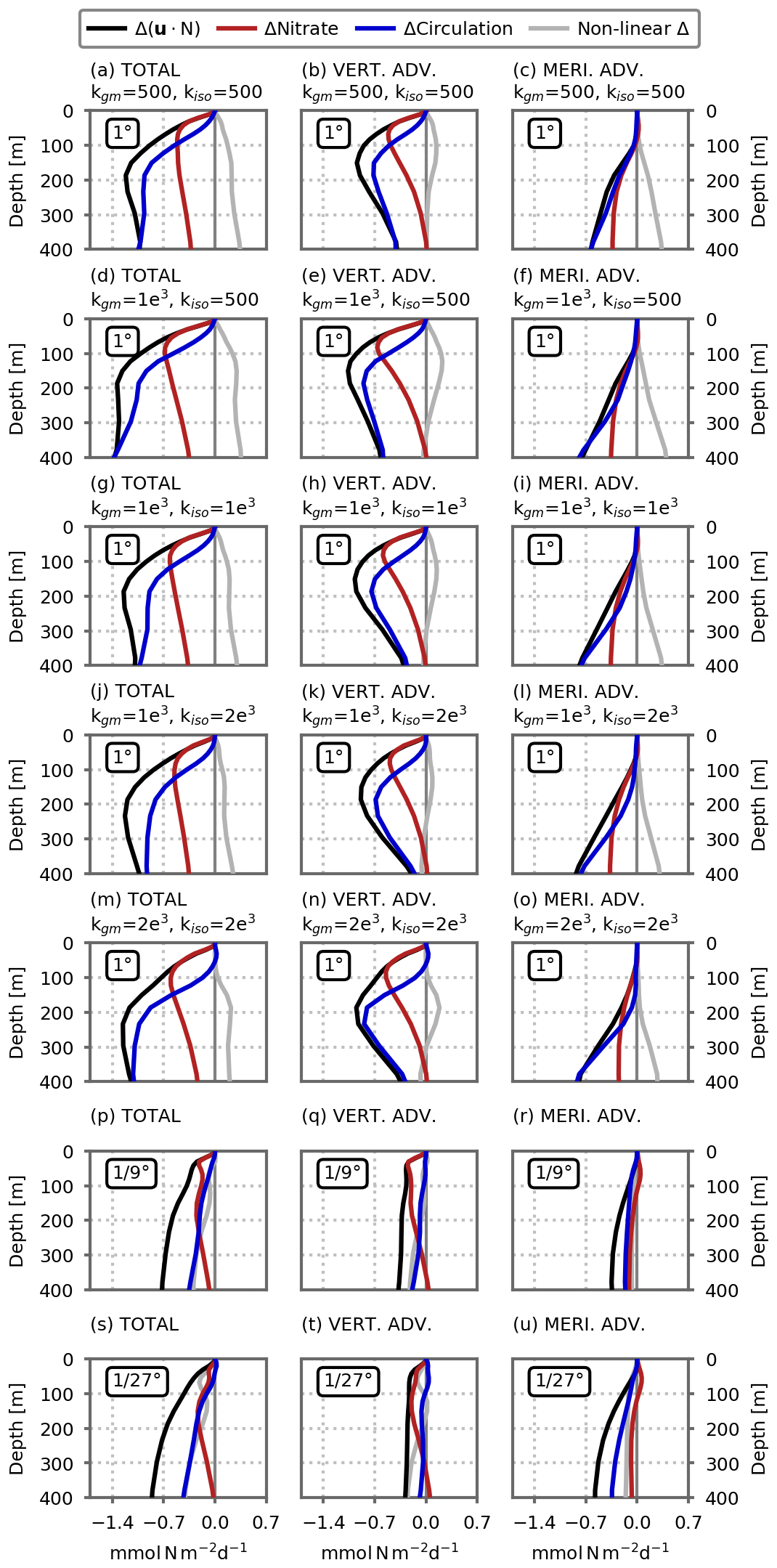
Figure A7Vertical profiles of changes in advective nitrate supplies (black lines, ) broken into the nitrate distribution change term (red lines), circulation change term (blue lines) and residual non-linear term (gray lines). Changes are cumulated between the surface and depth D in the model's subpolar box (dashed black lines in Fig. 3) and plotted against D. Change is the difference between climate change and preindustrial control simulations For details, see the Methodology section, Eqs. (3) to (6). The first column shows total advective fluxes which are the sum of the vertical advective fluxes at depth D (second column) and the meridional advective fluxes at the southern border (third column). Panels (a)–(o) show the five 1∘ resolution configurations, and (p)–(u) show the and ∘ resolution configurations. All figures show the average over the last 5 years of the simulations (years 66 to 70).
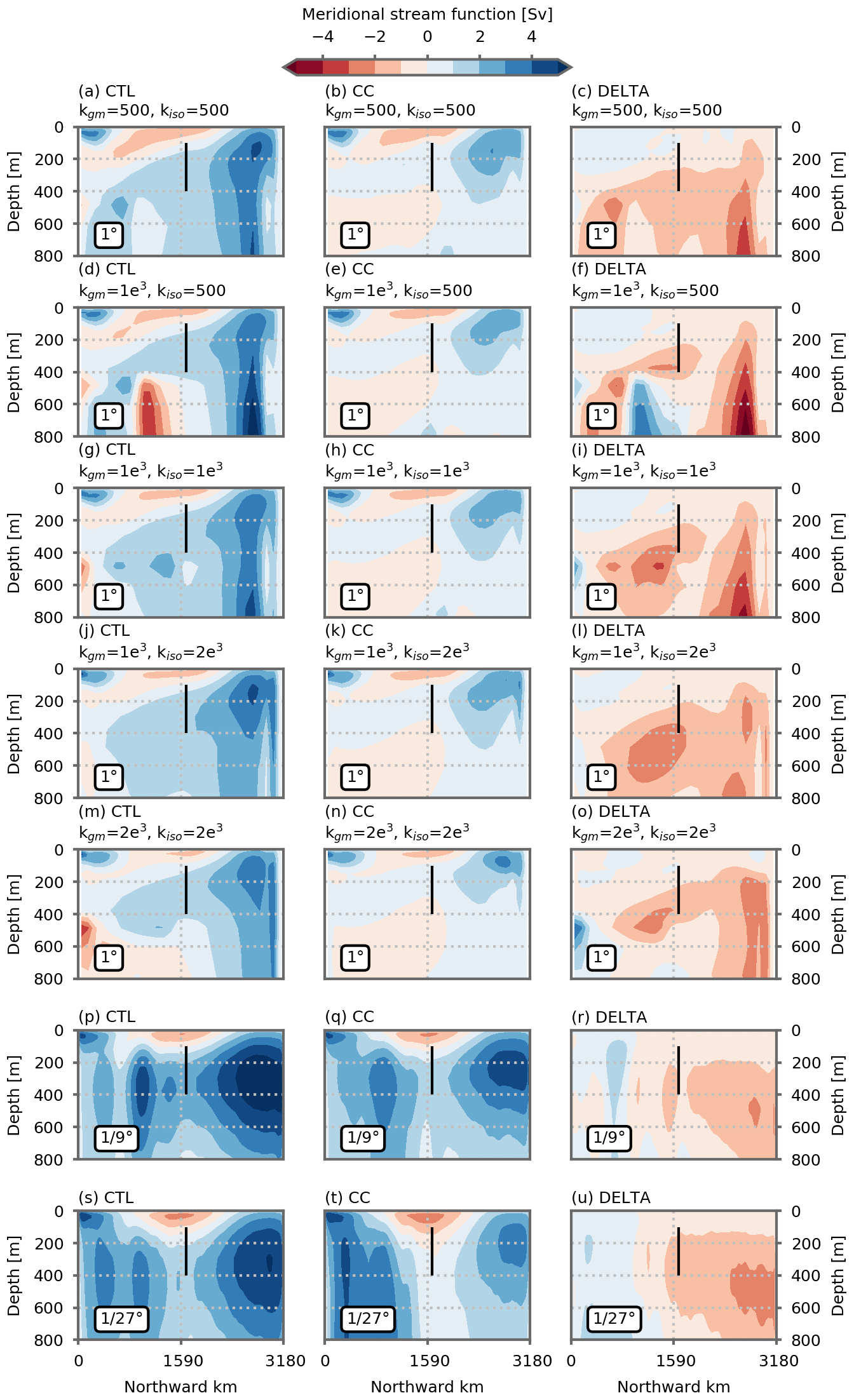
Figure A8Meridional stream functions (Sv) in the preindustrial control simulation (first column) and climate change simulations (second column) and the difference between the two (third column). Meridional stream functions are computed in z coordinates. The vertical black lines range from 100 to 400 m depth and show the area through which we diagnose the water flow between the two gyres. Panels (a)–(o) show the five 1∘ resolution configurations, and (p)–(u) show the and ∘ resolution configurations. All figures show the average over the last 5 years of the simulations (years 66 to 70).
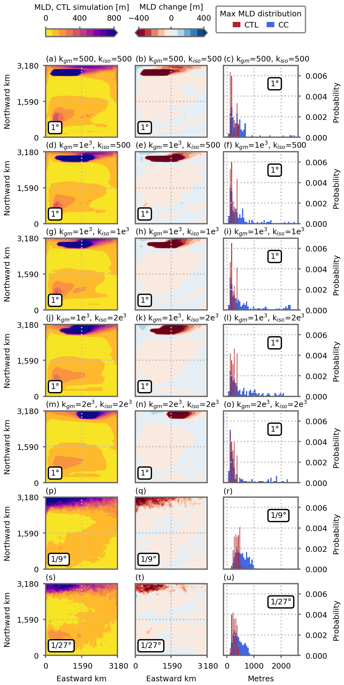
Figure A9Maximum depth of the mixed layer (meters) reached along the seasonal cycle (monthly averages) in the preindustrial control simulations (first column) and differences in the climate change simulations (second column). The third column shows distributions of maximum mixed-layer depth north of the model's subpolar box (dashed black lines in Fig. 3) in the preindustrial control simulations (blue bars) and the climate change simulations (red bars). Panels (a)–(o) show the five 1∘ resolution configurations, and (p)–(u) show the and ∘ resolution configurations. All figures show the average over the last 5 years of the simulations (years 66 to 70).

Figure A10Vertical distribution of the Brunt–Vaisala frequency across the domain (zonal mean, ) in the preindustrial control simulations (first column) and the climate change simulations (second column) and the difference between the two (third column). Panels (a)–(o) show the five 1∘ resolution configurations, and (p)–(u) show the and ∘ resolution configurations. All figures show the average over the last 5 years of the simulations (years 66 to 70).
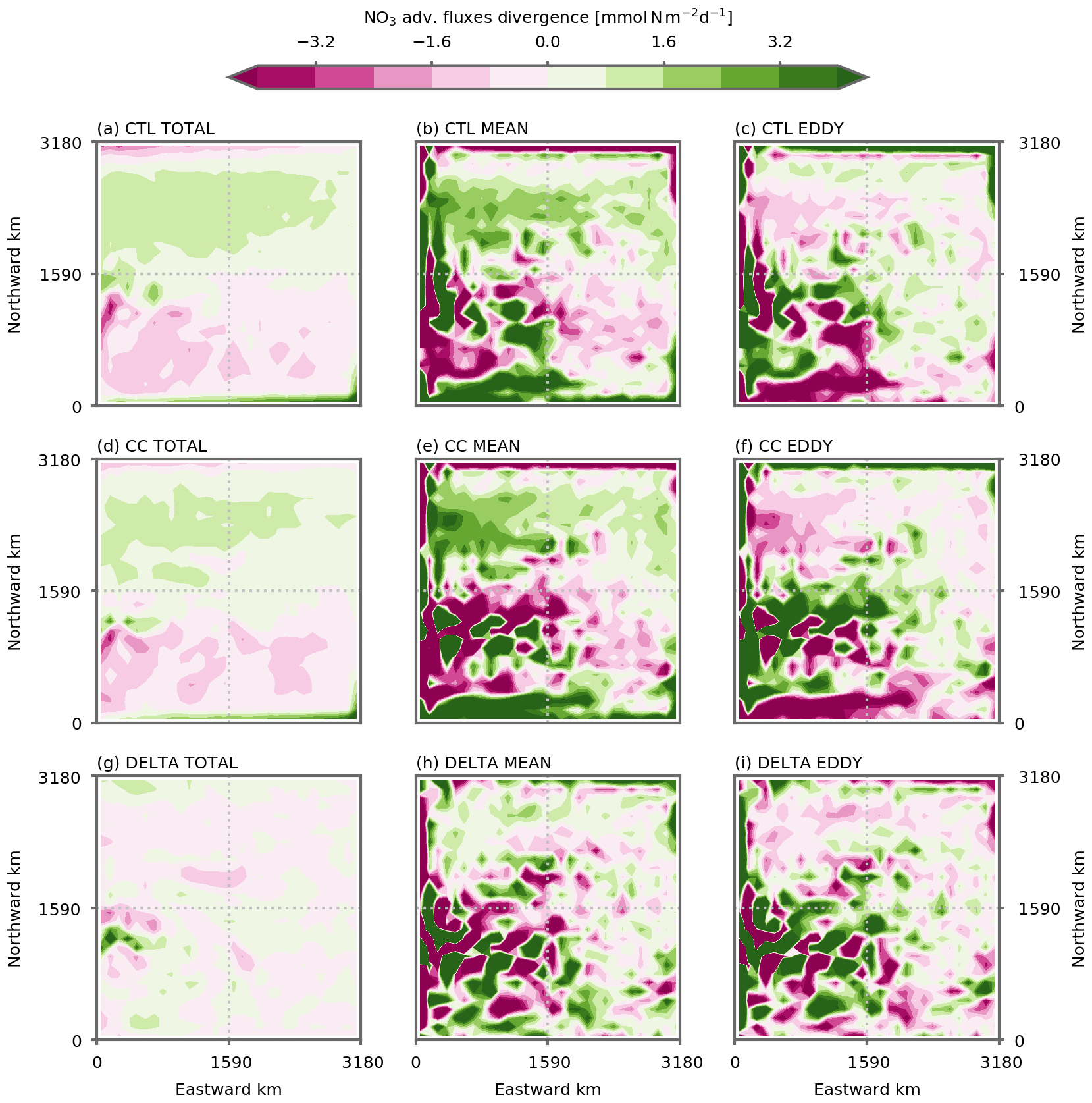
Figure A11Decomposition of the local divergence of the nitrate advective fluxes () into a mean component and a fluctuating eddy component, for the ∘ simulation. (a, d, g) Total local divergence, (b, e, h) mean component and (c, f, i) residual eddy component. (a–c) The preindustrial control simulations, (d–f) the climate change simulations and (g–i) the difference between the two. The total component is computed using 2 d averages; the mean component is computed using a spatio-temporal (1∘ and 1 year) average. The eddy component is the residual between the two. The decomposition is integrated vertically between the surface and 400 m depth and averaged over the last 5 years of each simulation (years 66 to 70). Details of the decomposition are in the Methodology section. Positive values indicate an input of nitrate.
Python scripts used for analyzing model's outputs and for producing the figures are available online at https://doi.org/10.5281/zenodo.5109751 (Couespel, 2019).
Due to the large volume of model output (16 TB), the data have not been deposited in a public repository. Data are available on request.
DC wrote the manuscript, conducted the simulations and performed the analysis. ML conceived the model experiments. All authors contributed to the writing.
The authors declare that they have no conflict of interest.
Publisher's note: Copernicus Publications remains neutral with regard to jurisdictional claims in published maps and institutional affiliations.
The authors thank Christian Ethe and Claude Talandier for their help in adapting the model configuration. The authors are grateful for stimulating discussions with Dan Whitt.
This research has been supported by the Agence Nationale de la Recherche (SOBUMS (grant no. ANR-16-CE01-0014)) and the European Commission's Horizon 2020 Framework Programme (CRESCENDO (grant no. 641816)).
This paper was edited by Akihiko Ito and reviewed by Scott C. Doney and Christopher Sabine.
Bahl, A., Gnanadesikan, A., and Pradal, M.-A. S.: Scaling global warming impacts on ocean ecosystems: Lessons from a suite of earth system models, Front. Mar. Sci., 7, 698, https://doi.org/10.3389/fmars.2020.00698, 2020. a
Beaulieu, C., Henson, S. A., Sarmiento, J. L., Dunne, J. P., Doney, S. C., Rykaczewski, R. R., and Bopp, L.: Factors challenging our ability to detect long-term trends in ocean chlorophyll, Biogeosciences, 10, 2711–2724, https://doi.org/10.5194/bg-10-2711-2013, 2013. a
Bindoff, N. L., Cheung, W. W., Kairo, J., Arístegui, J., Guinder, V., Hallberg, R., Hilmi, N., Jiao, N., Karim, M., Levin, L., O'Donoghue, S., Purca Cuicapusa, S., Rinkevich, B., Suga, T., Tagliabue, A., and Williamson, P.: Changing ocean, marine ecosystems, and dependent communities, in: IPCC special report on the ocean and cryosphere in a changing climate, section: 5, edited by: Pörtner, H.-O., Roberts, D., Masson-Delmotte, V., Zhai, P., Tignor, M., Poloczanska, E., Mintenbeck, K., Alegria, A., Nicolai, M., Okem, A., Petzold, J., Rama, B., and Weyer, N., in press, 2019. a, b, c, d
Bonan, G. B. and Doney, S. C.: Climate, ecosystems, and planetary futures: The challenge to predict life in Earth system models, Science, 359, eaam8328, https://doi.org/10.1126/science.aam8328, 2018. a
Bopp, L., Resplandy, L., Orr, J. C., Doney, S. C., Dunne, J. P., Gehlen, M., Halloran, P., Heinze, C., Ilyina, T., Séférian, R., Tjiputra, J., and Vichi, M.: Multiple stressors of ocean ecosystems in the 21st century: projections with CMIP5 models, Biogeosciences, 10, 6225–6245, https://doi.org/10.5194/bg-10-6225-2013, 2013. a
Boyce, D. G., Lewis, M. R., and Worm, B.: Global phytoplankton decline over the past century, Nature, 466, 591–596, https://doi.org/10.1038/nature09268, 2010. a
Bras, I. L., Straneo, F., Muilwijk, M., Smedsrud, L. H., Li, F., Lozier, M. S., and Holliday, N. P.: How Much Arctic Fresh Water Participates in the Subpolar Overturning Circulation?, J. Phys. Oceanogr., 51, 955–973, https://doi.org/10.1175/JPO-D-20-0240.1, 2021. a, b
Bronselaer, B., Zanna, L., Munday, D. R., and Lowe, J.: The influence of Southern Ocean winds on the North Atlantic carbon sink, Global Biogeochem. Cy., 30, 844–858, https://doi.org/10.1002/2015GB005364, 2016. a
Cavicchioli, R., Ripple, W. J., Timmis, K. N., Azam, F., Bakken, L. R., Baylis, M., Behrenfeld, M. J., Boetius, A., Boyd, P. W., Classen, A. T., Crowther, T. W., Danovaro, R., Foreman, C. M., Huisman, J., Hutchins, D. A., Jansson, J. K., Karl, D. M., Koskella, B., Mark Welch, D. B., Martiny, J. B., Moran, M. A., Orphan, V. J., Reay, D. S., Remais, J. V., Rich, V. I., Singh, B. K., Stein, L. Y., Stewart, F. J., Sullivan, M. B., van Oppen, M. J., Weaver, S. C., Webb, E. A., and Webster, N. S.: Scientists' warning to humanity: microorganisms and climate change, Nat. Rev. Microbiol., 17, 569–586, https://doi.org/10.1038/s41579-019-0222-5, 2019. a
Chanut, J., Barńier, B., Large, W., Debreu, L., Penduff, T., Molines, J. M., and Mathiot, P.: Mesoscale eddies in the Labrador Sea and their contribution to convection and restratification, J. Phys. Oceanogr., 38, 1617–1643, https://doi.org/10.1175/2008JPO3485.1, 2008. a
Chassignet, E. P. and Marshall, D. P.: Gulf Stream separation in numerical ocean models, Ocean Modeling in an Eddying Regime, 177, 39–61, https://doi.org/10.1029/177GM05, Union, 2008. a
Chassignet, E. P. and Xu, X.: Impact of horizontal resolution (∘ to ∘) on gulf stream separation, penetration, and variability, J. Phys. Oceanogr., 47, 1999–2021, https://doi.org/10.1175/JPO-D-17-0031.1, 2017. a
Chassot, E., Bonhommeau, S., Dulvy, N. K., Mélin, F., Watson, R., Gascuel, D., and Le Pape, O.: Global marine primary production constrains fisheries catches, Ecol. Lett., 13, 495–505, https://doi.org/10.1111/j.1461-0248.2010.01443.x, 2010. a
Couespel, D.: Oceanic primary production decline halved in eddy-resolving simulations of global warming: python scripts for model's output analysis and figure production, Zenodo [data set], https://doi.org/10.5281/zenodo.5109751, last access: 21 July 2021.
Delworth, T. L. and Zeng, F.: Simulated impact of altered southern hemisphere winds on the atlantic meridional overturning circulation, Geophys. Res. Lett., 35, L20708, https://doi.org/10.1029/2008GL035166, 2008. a
Delworth, T. L., Rosati, A., Anderson, W., Adcroft, A. J., Balaji, V., Benson, R., Dixon, K., Griffies, S. M., Lee, H.-C., Pacanowski, R. C., Vecchi, G. A., Wittenberg, A. T., Zeng, F., and Zhang, R.: Simulated climate and climate change in the GFDL CM2.5 high-resolution coupled climate model, J. Climate, 25, 2755–2781, https://doi.org/10.1175/JCLI-D-11-00316.1, 2012. a, b
Doney, S. C.: Oceanography: Plankton in a warmer world, Nature, 444, 695–696, https://doi.org/10.1038/444695a, 2006. a
Eden, C. and Greatbatch, R. J.: Towards a mesoscale eddy closure, Ocean Model., 20, 223–239, https://doi.org/10.1016/j.ocemod.2007.09.002, 2008. a
Falkowski, P. G., Barber, R. T., and Smetacek, V.: Biogeochemical controls and feedbacks on ocean primary production, Science, 281, 200–206, https://doi.org/10.1126/science.281.5374.200, 1998. a
Farneti, R. and Delworth, T. L.: The role of mesoscale eddies in the remote oceanic response to altered southern hemisphere winds, J. Phys. Oceanogr., 40, 2348–2354, https://doi.org/10.1175/2010JPO4480.1, 2010. a
Farneti, R., Delworth, T. L., Rosati, A. J., Griffies, S. M., and Zeng, F.: The role of mesoscale eddies in the rectification of the Southern ocean response to climate change, J. Phys. Oceanogr., 40, 1539–1557, https://doi.org/10.1175/2010JPO4353.1, 2010. a, b
Field, C. B., Behrenfeld, M. J., Randerson, J. T., and Falkowski, P. G.: Primary production of the biosphere: Integrating terrestrial and oceanic components, Science, 281, 237–240, https://doi.org/10.1126/science.281.5374.237, 1998. a
Fox-Kemper, B., Ferrari, R., and Hallberg, R.: Parameterization of mixed layer eddies. Part I: Theory and diagnosis, J. Phys. Oceanogr., 38, 1145–1165, https://doi.org/10.1175/2007JPO3792.1, , 2008. a
Friedland, K. D., Stock, C., Drinkwater, K. F., Link, J. S., Leaf, R. T., Shank, B. V., Rose, J. M., Pilskaln, C. H., and Fogarty, M. J.: Pathways between primary production and fisheries yields of large marine ecosystems, PLoS ONE, 7, e28945, https://doi.org/10.1371/journal.pone.0028945, 2012. a
Fu, W., Randerson, J. T., and Moore, J. K.: Climate change impacts on net primary production (NPP) and export production (EP) regulated by increasing stratification and phytoplankton community structure in the CMIP5 models, Biogeosciences, 13, 5151–5170, https://doi.org/10.5194/bg-13-5151-2016, 2016. a, b
Gent, P. R. and McWilliams, J. C.: Isopycnal mixing in ocean circulation models, J. Phys. Oceanogr., 20, 150–160, https://doi.org/10.1175/1520-0485(1990)020<0150:IMIOCM>2.0.CO;2, 1990. a, b, c, d
Gregory, J. M., Dixon, K. W., Stouffer, R. J., Weaver, A. J., Driesschaert, E., Eby, M., Fichefet, T., Hasumi, H., Hu, A., Jungclaus, J. H., Kamenkovich, I. V., Levermann, A., Montoya, M., Murakami, S., Nawrath, S., Oka, A., Sokolov, A. P., and Thorpe, R. B.: A model intercomparison of changes in the Atlantic thermohaline circulation in response to increasing atmospheric CO2 concentration, Geophys. Res. Lett., 32, L12703, https://doi.org/10.1029/2005GL023209, 2005. a
Gula, J., Molemaker, M. J., and McWilliams, J. C.: Submesoscale dynamics of a gulf stream frontal eddy in the south atlantic bight, J. Phys. Oceanogr., 46, 305–325, https://doi.org/10.1175/JPO-D-14-0258.1, 2016. a
Gutjahr, O., Putrasahan, D., Lohmann, K., Jungclaus, J. H., von Storch, J.-S., Brüggemann, N., Haak, H., and Stössel, A.: Max Planck Institute Earth System Model (MPI-ESM1.2) for the High-Resolution Model Intercomparison Project (HighResMIP), Geosci. Model Dev., 12, 3241–3281, https://doi.org/10.5194/gmd-12-3241-2019, 2019. a
Haarsma, R. J., Roberts, M. J., Vidale, P. L., Senior, C. A., Bellucci, A., Bao, Q., Chang, P., Corti, S., Fučkar, N. S., Guemas, V., von Hardenberg, J., Hazeleger, W., Kodama, C., Koenigk, T., Leung, L. R., Lu, J., Luo, J.-J., Mao, J., Mizielinski, M. S., Mizuta, R., Nobre, P., Satoh, M., Scoccimarro, E., Semmler, T., Small, J., and von Storch, J.-S.: High Resolution Model Intercomparison Project (HighResMIP v1.0) for CMIP6, Geosci. Model Dev., 9, 4185–4208, https://doi.org/10.5194/gmd-9-4185-2016, 2016. a
Henson, S. A., Beaulieu, C., and Lampitt, R.: Observing climate change trends in ocean biogeochemistry: when and where, Glob. Change Biol., 22, 1561–1571, https://doi.org/10.1111/gcb.13152, 2016. a
Hirschi, J. J., Barnier, B., Böning, C., Biastoch, A., Blaker, A. T., Coward, A., Danilov, S., Drijfhout, S., Getzlaff, K., Griffies, S. M., Hasumi, H., Hewitt, H., Iovino, D., Kawasaki, T., Kiss, A. E., Koldunov, N., Marzocchi, A., Mecking, J. V., Moat, B., Molines, J., Myers, P. G., Penduff, T., Roberts, M., Treguier, A., Sein, D. V., Sidorenko, D., Small, J., Spence, P., Thompson, L., Weijer, W., and Xu, X.: The Atlantic meridional overturning circulation in high resolution models, J. Geophys. Res.-Oceans, 125, e2019JC015522, https://doi.org/10.1029/2019JC015522, 2020. a, b, c
IPBES: Global assessment report on biodiversity and ecosystem services of the Intergovernmental Science-Policy Platform on Biodiversity and Ecosystem Services, IPBES secretariat/IPBES, edited by: Brondizio, E. S. Settele, J., Díaz, S., and Ngo, H. T., Bonn, Germany, available at: https://ipbes.net/global-assessment (last access: 14 July 2021), https://doi.org/10.5281/zenodo.3831674, 2019. a, b
IPCC: IPCC special report on the ocean and cryosphere in a changing climate, IPCC, edited by: Pörtner, H.-O., Roberts, D. C., Masson-Delmotte, V., Zhai, P., Tignor, M., Poloczanska, E., Mintenbeck, K., Alegría, A., Nicolai, M., Okem, A., Petzold, J., Rama, B., and Weyer, N. M., available at: https://www.ipcc.ch/srocc/ (last access: 14 July 2021), in press, 2019. a, b
Jackson, L. C., Roberts, M. J., Hewitt, H. T., Iovino, D., Koenigk, T., Meccia, V. L., Roberts, C. D., Ruprich-Robert, Y., and Wood, R. A.: Impact of ocean resolution and mean state on the rate of AMOC weakening, Clim. Dynam., 55, 1711–1732, https://doi.org/10.1007/s00382-020-05345-9, 2020. a, b
Karleskind, P., Lévy, M., and Mémery, L.: Modifications of mode water properties by sub-mesoscales in a bio-physical model of the Northeast Atlantic, Ocean Model., 39, 47–60, https://doi.org/10.1016/j.ocemod.2010.12.003, 2011. a
Klocker, A.: Opening the window to the Southern Ocean: The role of jet dynamics, Sci. Adv., 4, eaao4719, https://doi.org/10.1126/sciadv.aao4719, 2018. a
Krémeur, A. S., Lévy, M., Aumont, O., and Reverdin, G.: Impact of the subtropical mode water biogeochemical properties on primary production in the North Atlantic: New insights from an idealized model study, J. Geophys. Res.-Oceans, 114, C07019, https://doi.org/10.1029/2008JC005161, 2009. a
Kwiatkowski, L., Torres, O., Bopp, L., Aumont, O., Chamberlain, M., Christian, J. R., Dunne, J. P., Gehlen, M., Ilyina, T., John, J. G., Lenton, A., Li, H., Lovenduski, N. S., Orr, J. C., Palmieri, J., Santana-Falcón, Y., Schwinger, J., Séférian, R., Stock, C. A., Tagliabue, A., Takano, Y., Tjiputra, J., Toyama, K., Tsujino, H., Watanabe, M., Yamamoto, A., Yool, A., and Ziehn, T.: Twenty-first century ocean warming, acidification, deoxygenation, and upper-ocean nutrient and primary production decline from CMIP6 model projections, Biogeosciences, 17, 3439–3470, https://doi.org/10.5194/bg-17-3439-2020, 2020. a, b, c, d
Laufkötter, C., Vogt, M., Gruber, N., Aita-Noguchi, M., Aumont, O., Bopp, L., Buitenhuis, E., Doney, S. C., Dunne, J., Hashioka, T., Hauck, J., Hirata, T., John, J., Le Quéré, C., Lima, I. D., Nakano, H., Seferian, R., Totterdell, I., Vichi, M., and Völker, C.: Drivers and uncertainties of future global marine primary production in marine ecosystem models, Biogeosciences, 12, 6955–6984, https://doi.org/10.5194/bg-12-6955-2015, 2015. a, b
Letscher, R. T., Primeau, F., and Moore, J. K.: Nutrient budgets in the subtropical ocean gyres dominated by lateral transport, Nat. Geosci., 9, 815–819, https://doi.org/10.1038/ngeo2812, 2016. a
Lewandowska, A. M., Boyce, D. G., Hofmann, M., Matthiessen, B., Sommer, U., and Worm, B.: Effects of sea surface warming on marine plankton, Ecol. Lett., 17, 614–623, https://doi.org/10.1111/ele.12265, 2014. a, b
Li, Q., Lee, S., and Griesel, A.: Eddy fluxes and jet-scale overturning circulations in the Indo–Western pacific southern ocean, J. Phys. Oceanogr., 46, 2943–2959, https://doi.org/10.1175/JPO-D-15-0241.1, 2016. a
Lique, C. and Thomas, M. D.: Latitudinal shift of the Atlantic Meridional Overturning Circulation source regions under a warming climate, Nat. Clim. Change, 8, 1013–1020, https://doi.org/10.1038/s41558-018-0316-5, 2018. a
Lotze, H. K., Tittensor, D. P., Bryndum-Buchholz, A., Eddy, T. D., Cheung, W. W., Galbraith, E. D., Barange, M., Barrier, N., Bianchi, D., Blanchard, J. L., Bopp, L., Büchner, M., Bulman, C. M., Carozza, D. A., Christensen, V., Coll, M., Dunne, J. P., Fulton, E. A., Jennings, S., Jones, M. C., Mackinson, S., Maury, O., Niiranen, S., Oliveros-Ramos, R., Roy, T., Fernandes, J. A., Schewe, J., Shin, Y. J., Silva, T. A., Steenbeek, J., Stock, C. A., Verley, P., Volkholz, J., Walker, N. D., and Worm, B.: Global ensemble projections reveal trophic amplification of ocean biomass declines with climate change, P. Natl. Acad. Sci. USA, 116, 12907–12912, https://doi.org/10.1073/pnas.1900194116, 2019. a
Lozier, M. S.: Overturning in the north atlantic, Annu. Rev. Mar. Sci., 4, 291–315, https://doi.org/10.1146/annurev-marine-120710-100740, 2012. a
Lozier, M. S., Dave, A. C., Palter, J. B., Gerber, L. M., and Barber, R. T.: On the relationship between stratification and primary productivity in the North Atlantic, Geophys. Res. Lett., 38, L18609, https://doi.org/10.1029/2011GL049414, 2011. a
Lévy, M.: Nutrients in remote mode, Nature, 437, 628–631, https://doi.org/10.1038/437628a, 2005. a, b
Lévy, M. and Martin, A. P.: The influence of mesoscale and submesoscale heterogeneity on ocean biogeochemical reactions, Global Biogeochem. Cy., 27, 1139–1150, https://doi.org/10.1002/2012GB004518, 2013. a, b
Lévy, M., Estublier, A., and Madec, G.: Choice of an advection scheme for biogeochemical models, Geophysical Research Letters, 28, 3725–3728, https://doi.org/10.1029/2001GL012947, 2001. a
Lévy, M., Klein, P., Tréguier, A. M., Iovino, D., Madec, G., Masson, S., and Takahashi, K.: Modifications of gyre circulation by sub-mesoscale physics, Ocean Model., 34, 1–15, https://doi.org/10.1016/j.ocemod.2010.04.001, 2010. a, b, c, d
Lévy, M., Ferrari, R., Frank J Millero, G. P. J. E. D., Martin, A. P., and Rivière, P.: Bringing physics to life at the submesoscale, Geophys. Res. Lett., 39, L14602, https://doi.org/10.1029/2012GL052756, 2012a. a
Lévy, M., Iovino, D., Resplandy, L., Klein, P., Madec, G., Treguier, A.-M., Masson, S., and Takahashi, T.: Large-scale impacts of submesoscale dynamics on phytoplankton: Local and remote effects, Ocean Model., 43–44, 77–93, https://doi.org/10.1016/j.ocemod.2011.12.003, 2012b. a, b, c
Lévy, M., Franks, P. J., and Smith, K. S.: The role of submesoscale currents in structuring marine ecosystems, Nat. Commun., 9, 4758, https://doi.org/10.1038/s41467-018-07059-3, 2018. a
Madec, G., Bourdallé-Badie, R., Bouttier, P.-A., Bricaud, C., Bruciaferri, D., Calvert, D., Chanut, J., Clementi, E., Coward, A., Delrosso, D., Ethé, C., Flavoni, S., Graham, T., Harle, J., Iovino, D., Lea, D., Lévy, C., Lovato, T., Martin, N., Masson, S., Mocavero, S., Paul, J., Rousset, C., Storkey, D., Storto, A., and Vancoppenolle, M.: NEMO ocean engine, Notes du Pôle de modélisation de l'Institut Pierre-Simon Laplace (IPSL), Zenodo, https://doi.org/10.5281/ZENODO.1472492, 2017. a, b
Mahadevan, A.: The impact of submesoscale physics on primary productivity of plankton, Annu. Rev. Mar. Sci., 8, 161–184, https://doi.org/10.1146/annurev-marine-010814-015912, publisher: Annual Reviews, 2016. a
Mak, J., Marshall, D. P., Maddison, J. R., and Bachman, S. D.: Emergent eddy saturation from an energy constrained eddy parameterisation, Ocean Model., 112, 125–138, https://doi.org/10.1016/j.ocemod.2017.02.007, 2017. a, b, c, d
Mak, J., Maddison, J. R., Marshall, D. P., and Munday, D. R.: Implementation of a geometrically informed and energetically constrained mesoscale eddy parameterization in an ocean circulation model, J. Phys. Oceanogr., 48, 2363–2382, https://doi.org/10.1175/JPO-D-18-0017.1, 2018. a, b, c
Marshall, D. P., Maddison, J. R., and Berloff, P. S.: A framework for parameterizing eddy potential vorticity fluxes, J. Phys. Oceanogr., 42, 539–557, https://doi.org/10.1175/JPO-D-11-048.1, 2012. a, b, c
McGillicuddy Jr., D. J.: Mechanisms of physical-biological-biogeochemical interaction at the oceanic mesoscale, Annu. Rev. Mar. Sci., 8, 125–159, https://doi.org/10.1146/annurev-marine-010814-015606, 2016. a
McKinley, G. A., Ritzer, A. L., and Lovenduski, N. S.: Mechanisms of northern North Atlantic biomass variability, Biogeosciences, 15, 6049–6066, https://doi.org/10.5194/bg-15-6049-2018, 2018. a
McWilliams, J. C.: Submesoscale currents in the ocean, P. Roy. Soc. A, 472, 20160117, https://doi.org/10.1098/rspa.2016.0117, 2016. a
Meredith, M. P., Garabato, A. C. N., Hogg, A. M., and Farneti, R.: Sensitivity of the overturning circulation in the southern ocean to decadal changes in wind forcing, J. Climate, 25, 99–110, https://doi.org/10.1175/2011JCLI4204.1, 2012. a, b
Moore, J. K., Fu, W., Primeau, F., Britten, G. L., Lindsay, K., Long, M., Doney, S. C., Mahowald, N., Hoffman, F., and Randerson, J. T.: Sustained climate warming drives declining marine biological productivity, Science, 359, 113–1143, https://doi.org/10.1126/science.aao6379, 2018. a
Munday, D. R., Johnson, H. L., and Marshall, D. P.: Eddy saturation of equilibrated circumpolar currents, J. Phys. Oceanogr., 43, 507–532, https://doi.org/10.1175/JPO-D-12-095.1, 2013. a, b, c
Munday, D. R., Johnson, H. L., and Marshall, D. P.: Impacts and effects of mesoscale ocean eddies on ocean carbon storage and atmospheric pCO2, Global Biogeochem. Cy., 28, 877–896, https://doi.org/10.1002/2014GB004836, 2014. a
Olonscheck, D., Hofmann, M., Worm, B., and Schellnhuber, H. J.: Decomposing the effects of ocean warming on chlorophyll a concentrations into physically and biologically driven contributions, Environ. Res. Lett., 8, 14043, https://doi.org/10.1088/1748-9326/8/1/014043, 2013. a, b
Palter, J. B. and Lozier, M. S.: On the source of Gulf Stream nutrients, J. Geophys. Res.-Oceans, 113, C06018, https://doi.org/10.1029/2007JC004611, 2008. a
Palter, J. B., Lozier, M. S., and Barber, R. T.: The effect of advection on the nutrient reservoir in the North Atlantic subtropical gyre, Nature, 437, 687–692, https://doi.org/10.1038/nature03969, 2005. a
Pauly, D. and Christensen, V.: Primary production required to sustain global fisheries, Nature, 374, 255–257, https://doi.org/10.1038/374255a0, 1995. a
Polovina, J. J., Howell, E. A., and Abecassis, M.: Ocean's least productive waters are expanding, Geophys. Res. Lett., 35, L03618, https://doi.org/10.1029/2007GL031745, 2008. a
Resplandy, L., Lévy, M., and McGillicuddy Jr., D. J.: Effects of Eddy‐Driven subduction on ocean biological carbon pump, Global Biogeochem. Cy., 33, 1071–1084, https://doi.org/10.1029/2018GB006125, 2019. a
Roberts, M. J., Banks, H., Gedney, N., Gregory, J., Hill, R., Mullerworth, S., Pardaens, A., Rickard, G., Thorpe, R., Wood, R., Roberts, M. J., Banks, H., Gedney, N., Gregory, J., Hill, R., Mullerworth, S., Pardaens, A., Rickard, G., Thorpe, R., and Wood, R.: Impact of an eddy-permitting ocean resolution on control and climate change simulations with a global coupled GCM, J. Climate, 17, 3–20, https://doi.org/10.1175/1520-0442(2004)017<0003:IOAEOR>2.0.CO;2, 2004. a, b
Roberts, M. J., Jackson, L. C., Roberts, C. D., Meccia, V., Docquier, D., Koenigk, T., Ortega, P., Moreno-Chamarro, E., Bellucci, A., Coward, A., Drijfhout, S., Exarchou, E., Gutjahr, O., Hewitt, H., Iovino, D., Lohmann, K., Putrasahan, D., Schiemann, R., Seddon, J., Terray, L., Xu, X., Zhang, Q., Chang, P., Yeager, S. G., Castruccio, F. S., Zhang, S., and Wu, L.: Sensitivity of the Atlantic Meridional Overturning Circulation to Model Resolution in CMIP6 HighResMIP Simulations and Implications for Future Changes, J. Adv. Model. Earth Sy., 12, e2019MS002014, https://doi.org/10.1029/2019MS002014, 2020. a, b, c
Sarmiento, J. L. and Gruber, N.: Ocean biogeochemical dynamics, Princeton University Press, 2006. a
Spence, P., Saenko, O. A., Sijp, W., and England, M. H.: North atlantic climate response to lake agassiz drainage at coarse and ocean eddy-permitting resolutions, J. Climate, 26, 2651–2667, https://doi.org/10.1175/JCLI-D-11-00683.1, 2013. a, b
Steinacher, M., Joos, F., Frölicher, T. L., Bopp, L., Cadule, P., Cocco, V., Doney, S. C., Gehlen, M., Lindsay, K., Moore, J. K., Schneider, B., and Segschneider, J.: Projected 21st century decrease in marine productivity: a multi-model analysis, Biogeosciences, 7, 979–1005, https://doi.org/10.5194/bg-7-979-2010, 2010. a, b, c
Stock, C. A., John, J. G., Rykaczewski, R. R., Asch, R. G., Cheung, W. W., Dunne, J. P., Friedland, K. D., Lam, V. W., Sarmiento, J. L., and Watson, R. A.: Reconciling fisheries catch and ocean productivity, P. Natl. Acad. Sci. USA, 114, E1441–E1449, https://doi.org/10.1073/pnas.1610238114, 2017. a
Séférian, R., Berthet, S., Yool, A., Palmiéri, J., Bopp, L., Tagliabue, A., Kwiatkowski, L., Aumont, O., Christian, J., Dunne, J., Gehlen, M., Ilyina, T., John, J. G., Li, H., Long, M. C., Luo, J. Y., Nakano, H., Romanou, A., Schwinger, J., Stock, C., Santana-Falcón, Y., Takano, Y., Tjiputra, J., Tsujino, H., Watanabe, M., Wu, T., Wu, F., and Yamamoto, A.: Tracking improvement in simulated marine biogeochemistry between CMIP5 and CMIP6, Current Climate Change Reports, 95–119, https://doi.org/10.1007/s40641-020-00160-0, 2020. a
Tagklis, F., Ito, T., and Bracco, A.: Modulation of the North Atlantic deoxygenation by the slowdown of the nutrient stream, Biogeosciences, 17, 231–244, https://doi.org/10.5194/bg-17-231-2020, 2020. a, b, c
Tamarin, T., Maddison, J. R., Heifetz, E., and Marshall, D. P.: A geometric interpretation of eddy reynolds stresses in barotropic ocean jets, J. Phys. Oceanogr., 46, 2285–2307, https://doi.org/10.1175/JPO-D-15-0139.1, 2016. a
Tokarska, K. B., Stolpe, M. B., Sippel, S., Fischer, E. M., Smith, C. J., Lehner, F., and Knutti, R.: Past warming trend constrains future warming in CMIP6 models, Sci. Adv., 6, eaaz9549, https://doi.org/10.1126/sciadv.aaz9549, 2020. a, b
Uchida, T., Balwada, D., Abernathey, R., McKinley, G., Smith, S., and Lévy, M.: The contribution of submesoscale over mesoscale eddy iron transport in the open southern ocean, J. Adv. Model. Earth Sy., 11, 3934–3958, https://doi.org/10.1029/2019MS001805, Ltd, 2019. a
Uchida, T., Balwada, D., Abernathey, R. P., McKinley, G. A., Smith, S. K., and Lévy, M.: Vertical eddy iron fluxes support primary production in the open Southern Ocean, Nat. Commun., 11, 1–8, https://doi.org/10.1038/s41467-020-14955-0, 2020. a
Uchiyama, Y., Suzue, Y., and Yamazaki, H.: Eddy-driven nutrient transport and associated upper-ocean primary production along the Kuroshio, J. Geophys. Res.-Oceans, 122, 5046–5062, https://doi.org/10.1002/2017JC012847, 2017. a
van Westen, R. M. and Dijkstra, H. A.: Ocean eddies strongly affect global mean sea-level projections, Sci. Adv., 7, eabf1674, https://doi.org/10.1126/sciadv.abf1674, 2021. a, b
Volk, T. and Hoffert, M. I.: Ocean carbon pumps: Analysis of relative strengths and efficiencies in ocean-driven atmospheric CO2 changes, The Carbon Cycle and Atmospheric CO2: Natural Variations Archean to Present, 32, 99–110, https://doi.org/10.1029/GM032p0099, 1985. a
Weijer, W., Maltrud, M. E., Hecht, M. W., Dijkstra, H. A., and Kliphuis, M. A.: Response of the Atlantic Ocean circulation to Greenland Ice Sheet melting in a strongly-eddying ocean model, Geophys. Res. Lett., 39, L09606, https://doi.org/10.1029/2012GL051611, 2012. a
Wernand, M. R., van der Woerd, H. J., and Gieskes, W. W. C.: Trends in ocean colour and chlorophyll concentration from 1889 to 2000, worldwide, PLoS ONE, 8, e63766, https://doi.org/10.1371/journal.pone.0063766, 2013. a
Whitt, D. B.: On the role of the gulf stream in the changing atlantic nutrient circulation during the 21st century, in: Kuroshio current: Physical, biogeochemical, and ecosystem dynamics, geophysical monograph 243, edited by: Nagai, T., Saito, H., Suzuki, K., and Takahashi, M., 51–82, John Wiley & Sons, Inc., 1st Edn., https://doi.org/10.1002/9781119428428.ch4, 2019. a, b, c, d
Whitt, D. B. and Jansen, M. F.: Slower nutrient stream suppresses Subarctic Atlantic Ocean biological productivity in global warming, P. Natl. Acad. Sci. USA, 117, 15504–15510, https://doi.org/10.1073/pnas.2000851117, 2020. a, b, c
Williams, R. G., Roussenov, V., and Follows, M. J.: Nutrient streams and their induction into the mixed layer, Global Biogeochem. Cy., 20, GB1016, https://doi.org/10.1029/2005GB002586, 2006. a
Williams, R. G., McDonagh, E., Roussenov, V. M., Torres-Valdes, S., King, B., Sanders, R., and Hansell, D. A.: Nutrient streams in the North Atlantic: Advective pathways of inorganic and dissolved organic nutrients, Global Biogeochem. Cy., 25, GB4008, https://doi.org/10.1029/2010GB003853, 2011. a, b
Winton, M., Anderson, W. G., Delworth, T. L., Griffies, S. M., Hurlin, W. J., and Rosati, A.: Has coarse ocean resolution biased simulations of transient climate sensitivity?, Geophys. Res. Lett., 41, 8522–8529, https://doi.org/10.1002/2014GL061523, 2014. a, b
Yang, H., Lohmann, G., Krebs‐Kanzow, U., Ionita, M., Shi, X., Sidorenko, D., Gong, X., Chen, X., and Gowan, E. J.: Poleward shift of the major ocean gyres detected in a warming climate, Geophys. Res. Lett., 47, e2019GL085868, https://doi.org/10.1029/2019GL085868, 2020. a
Zanna, L., Porta Mana, P. G. L., Anstey, J., David, T., and Bolton, T.: Scale-aware deterministic and stochastic parametrizations of eddy-mean flow interaction, Ocean Model., 111, 66–80, https://doi.org/10.1016/j.ocemod.2017.01.004, 2017. a, b, c, d, e