the Creative Commons Attribution 4.0 License.
the Creative Commons Attribution 4.0 License.
 | 09 Aug 2021
Temporal variability and driving factors of the carbonate system in the Aransas Ship Channel, TX, USA: a time series study
Melissa R. McCutcheon
Hongming Yao
Cory J. Staryk
Xinping Hu
The coastal ocean is affected by an array of co-occurring biogeochemical and anthropogenic processes, resulting in substantial heterogeneity in water chemistry, including carbonate chemistry parameters such as pH and partial pressure of CO2 (pCO2). To better understand coastal and estuarine acidification and air-sea CO2 fluxes, it is important to study baseline variability and driving factors of carbonate chemistry. Using both discrete bottle sample collection (2014–2020) and hourly sensor measurements (2016–2017), we explored temporal variability, from diel to interannual scales, in the carbonate system (specifically pH and pCO2) at the Aransas Ship Channel located in the northwestern Gulf of Mexico. Using other co-located environmental sensors, we also explored the driving factors of that variability. Both sampling methods demonstrated significant seasonal variability at the location, with highest pH (lowest pCO2) in the winter and lowest pH (highest pCO2) in the summer. Significant diel variability was also evident from sensor data, but the time of day with elevated pCO2 and depressed pH was not consistent across the entire monitoring period, sometimes reversing from what would be expected from a biological signal. Though seasonal and diel fluctuations were smaller than many other areas previously studied, carbonate chemistry parameters were among the most important environmental parameters for distinguishing between time of day and between seasons. It is evident that temperature, biological activity, freshwater inflow, and tide level (despite the small tidal range) are all important controls on the system, with different controls dominating at different timescales. The results suggest that the controlling factors of the carbonate system may not be exerted equally on both pH and pCO2 on diel timescales, causing separation of their diel or tidal relationships during certain seasons. Despite known temporal variability on shorter timescales, discrete sampling was generally representative of the average carbonate system and average air-sea CO2 flux on a seasonal and annual basis when compared with sensor data.
- Article
(546 KB) - Full-text XML
-
Supplement
(518 KB) - BibTeX
- EndNote


Coastal waters, especially estuaries, experience substantial spatial and temporal heterogeneity in water chemistry – including carbonate chemistry parameters such as pH and partial pressure of CO2 (pCO2) – due to the diversity of co-occurring biogeochemical and anthropogenic processes (Hofmann et al., 2011; Waldbusser and Salisbury, 2014). Carbonate chemistry is important because an addition of CO2 acidifies seawater, and acidification can negatively affect marine organisms (Barton et al., 2015; Bednaršek et al., 2012; Ekstrom et al., 2015; Gazeau et al., 2007; Gobler and Talmage, 2014). Additionally, despite the small surface area of coastal waters relative to the global ocean, coastal waters are recognized as important contributors to global carbon cycling (Borges, 2005; Cai, 2011; Laruelle et al., 2018).
While carbonate chemistry, acidification, and air-sea CO2 fluxes are relatively well studied and understood in open ocean environments, large uncertainties remain in coastal environments. Estuaries are especially challenging to fully understand because of the heterogeneity between and within estuaries that is driven by diverse processes operating on different timescales such as river discharge, nutrient and organic matter loading, stratification, and coastal upwelling (Jiang et al., 2013; Mathis et al., 2012). The traditional sampling method for carbonate system characterization involving discrete water sample collection and laboratory analysis is known to lead to biases in average pCO2 and CO2 flux calculations due to daytime sampling that neglects to capture diel variability (Li et al., 2018). Mean diel ranges in pH can exceed 0.1 unit in many coastal environments, and especially high diel ranges (even exceeding 1 pH unit) have been reported in biologically productive areas or areas with higher mean pCO2 (Challener et al., 2016; Cyronak et al., 2018; Schulz and Riebesell, 2013; Semesi et al., 2009; Yates et al., 2007). These diel ranges can far surpass the magnitude of the changes in open ocean surface waters that have occurred since the start of the industrial revolution and rival spatial variability in productive systems, indicating their importance for a full understanding of the carbonate system.
Despite the need for high-frequency measurements, sensor deployments have been limited in estuarine environments (especially compared to their extensive use in the open ocean) because of the challenges associated with highly variable salinities, biofouling, and sensor drift (Sastri et al., 2019). Carbonate chemistry monitoring in the Gulf of Mexico (GOM), has been relatively minimal compared to the United States east and west coasts. The GOM estuaries currently have less exposure to concerning levels of acidification than other estuaries because of their high temperatures (causing water to hold less CO2 and support high productivity year-round) and often suitable river chemistries (i.e., relatively high buffer capacity) (McCutcheon et al., 2019; Yao et al., 2020). However, respiration-induced acidification is present in both the open GOM (e. g., subsurface water influenced by the Mississippi River Plume and outer shelf region near the Flower Garden Banks National Marine Sanctuary) and GOM estuaries, and most estuaries in the northwestern GOM have also experienced long-term acidification (Cai et al., 2011; Hu et al., 2015, 2018; Kealoha et al., 2020; McCutcheon et al., 2019; Robbins and Lisle, 2018). This evidence of acidification as well as the relatively high CO2 efflux from the estuaries of the northwest GOM illustrates the necessity to study the baseline variability and driving factors of carbonate chemistry in the region. In this study, we explored temporal variability in the carbonate system in the Aransas Ship Channel (ASC) – a tidal inlet where the lagoonal estuaries meet the coastal waters in a semi-arid region of the northwestern GOM – using both discrete bottle sample collection and hourly sensor measurements, and we explored the driving factors of that variability using data from other co-located environmental sensors. The characterization of carbonate chemistry and consideration of regional drivers can provide context to acidification and its impacts and improved estimates of air-sea CO2 fluxes.
2.1 Location
Autonomous sensor monitoring and discrete water sample collections for laboratory analysis of carbonate system parameters were performed in ASC (located at 27∘50′17′′ N, 97∘3′1′′ W). ASC is one of the few permanent tidal inlets that intersect a string of barrier islands and connect the GOM coastal waters with the lagoonal estuaries in the northwest GOM (Fig. 1). ASC provides the direct connection between the northwestern GOM and the Mission-Aransas Estuary (Copano and Aransas Bays) to the north and Nueces Estuary (Nueces and Corpus Christi Bays) to the south (Fig. 1). The region is microtidal, with a small tidal range relative to many other estuaries, ranging from ∼ 0.6 m tides on the open coast to less than 0.3 m in upper estuaries (Montagna et al., 2011). Mission-Aransas Estuary (MAE) is fed by two small rivers, the Mission (1787 km2 drainage basin) and Aransas (640 km2 drainage basin) Rivers (http://waterdata.usgs.gov/, last access: 20 January 2020), which both experience low base flows punctuated by periodic high flows during storm events. MAE has an average residence time of one year (Solis and Powell, 1999), so there is a substantial lag between time of rainfall and riverine delivery to ASC in the lower estuary. A significant portion of riverine water flowing into the Aransas Bay originates from the larger rivers further northeast on the Texas coast via the Intracoastal Waterway (i.e., Guadalupe River (26 625 km2 drainage basin) feeds San Antonio Bay and has a much shorter residence time of nearly 50 d) (Solis and Powell, 1999; USGS, 2001).
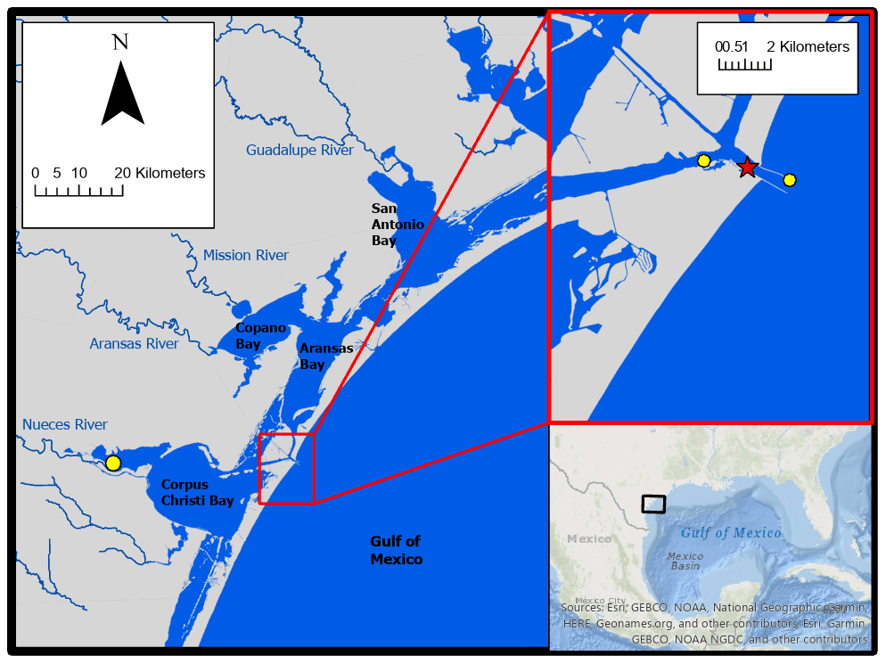
Figure 1Study area. The location of monitoring in the Aransas Ship Channel (red star) and the locations of NOAA stations used for wind data (yellow circles) are shown.
2.2 Continuous monitoring
Autonomous sensor monitoring (referred to throughout as continuous monitoring) of pH and pCO2 was conducted from 8 November 2016 to 23 August 2017 at the University of Texas Marine Science Institute's research pier in ASC. Hourly pH data were collected using an SAtlantic® SeaFET pH sensor (on a total pH scale) and hourly pCO2 data were collected using a Sunburst® SAMI-CO2. The pH and pCO2 sensors were placed in a flowthrough system that received surface water from ASC using a time-controlled diaphragm pump prior to each measurement. Hourly temperature and salinity data were measured by a YSI® 600OMS V2 sonde. All hourly data were single measurements taken on the hour. The average difference between sensor pH and discrete quality assurance samples measured spectrophotometrically in the lab was used to establish a correction factor (−0.05) across the entire sensor pH dataset. Note, this correction scheme was not ideal (Bresnahan et al., 2014) although less rigorous correction based on sensor and discrete pH values has also been used (Shadwick et al., 2019). Nevertheless, the overall good agreement between discrete and corresponding sensor pH values during the deployment period suggested that the SeaFET sensor remained stable. It is also worth noting that our monitoring setup remained free from biofouling during the 10-month period. We attribute this to the deployment design in which the high frequency movement of the pumping mechanisms in the diaphragm pump must have eliminated the influence of animal larvae. See Supplement for additional sensor deployment and quality assurance information.
2.3 Discrete sample collection and sample analysis
Long-term monitoring via discrete water sample collection was conducted at ASC from 2 May 2014 to 25 February 2020 (in addition to the discrete, quality assurance sample collections). A single, discrete, surface water sample was collected every two weeks during the summer months and monthly during the winter months from a small vessel at a station near (<20 m from) the sensor deployment. Water sample collection followed standard protocol for ocean carbonate chemistry studies (Dickson et al., 2007). Ground glass borosilicate bottles (250 mL) were filled with surface water and preserved with 100 µL saturated mercury chloride (HgCl2). Apiezon® grease was applied to the bottle stopper, which was then secured to the bottle using a rubber band and a nylon hose clamp.
These samples were used for laboratory dissolved inorganic carbon (DIC) and pH measurements. DIC was measured by injecting 0.5 mL of sample into 1 mL 10 % H3PO4 (balanced by 0.5 M NaCl) with a high-precision Kloehn syringe pump. The CO2 gas produced through sample acidification was then stripped using high-purity nitrogen gas and carried into a Li-Cor infrared gas detector. DIC analyses had a precision of 0.1 %. Certified Reference Material (CRM) was used to ensure the accuracy of the analysis (Dickson et al., 2003). For samples with salinity >20, pH was measured using a spectrophotometric method at 25 ± 0.1 ∘C (Carter et al., 2003) and the Douglas and Byrne (2017) equation. Analytical precision of the spectrophotometric method for pH measurement was ± 0.0004 pH units. A calibrated Orion Ross glass pH electrode was used to measure pH at 25 ± 0.1 ∘C for samples with salinity <20, and analytical precision was ± 0.01 pH units. All pH values obtained using the potentiometric method were converted to total scale at in situ temperature (Millero, 2001). Salinity of the discrete samples was measured using a benchtop salinometer calibrated by MilliQ water and a known salinity CRM. For discrete samples, pCO2 was calculated in CO2Sys for Excel using laboratory-measured salinity, DIC, pH, and in situ temperature for calculations. Carbonate speciation calculations were done using Millero (2010) carbonic acid dissociation constants (K1 and K2), Dickson (1990) bisulfate dissociation constant, and Uppström (1974) borate concentration.
2.4 Calculation of CO2 fluxes
Equation (1) was used for air-water CO2 flux calculations (Wanninkhof, 1992; Wanninkhof et al., 2009). Positive flux values indicate CO2 emission from the water into the atmosphere (the estuary acting as a source of CO2), and negative flux values indicate CO2 uptake by the water (the estuary acting as a sink for CO2).
where k is the gas transfer velocity (in m d−1), K0 (in mol L−1 atm−1) is the solubility constant of CO2 (Weiss, 1974), and pCO2,w andpCO2,a are the partial pressure of CO2 (in µatm) in the water and air, respectively.
We used the wind speed parameterization for gas transfer velocity (k) from Jiang et al. (2008) converted from cm h−1 to m d−1, which is thought to be the best estuarine parameterization at this time (Crosswell et al., 2017), as it is a composite of k over several estuaries. The calculation of k requires a wind speed at 10 m above the surface, so wind speeds measured at 3 m above the surface were converted using the power law wind profile (Hsu, 1994; Yao and Hu, 2017). To assess uncertainty, other parameterizations with direct applications to estuaries in the literature were also used to calculate CO2 flux (Raymond and Cole, 2001; Ho et al., 2006). We note that parameterization of k based on solely wind speed is flawed because several additional parameters can contribute to turbulence including turbidity, bottom-driven turbulence, water-side thermal convection, tidal currents, and fetch (Wanninkhof, 1992; Abril et al., 2009; Ho et al., 2104; Andersson et al., 2017), however it is currently the best option for this system given the limited investigations of CO2 flux and contributing factors in estuaries.
Hourly averaged wind speed data for use in CO2 flux calculations were retrieved from the NOAA-controlled Texas Coastal Ocean Observation Network (TCOON; https://tidesandcurrents.noaa.gov/tcoon.html, last access: 1 October 2020). Wind speed data from the nearest TCOON station (Port Aransas Station – located directly in ASC, <2 km inshore from our monitoring location) was prioritized when data were available. During periods of missing wind speed data at the Port Aransas Station, wind speed data from TCOON's Aransas Pass Station (<2 km offshore from monitoring location) were next used, and for all subsequent gaps, data from TCOON's Nueces Bay Station (∼ 40 km away) were used (Fig. 1; additional discussion of flux calculation and wind speed data can be found in the Supplement). For flux calculations from continuous monitoring data, each hourly measurement of pCO2 was paired with the corresponding hourly averaged wind speed. For flux calculations from discrete sample data, the pCO2 calculated for each sampled day was paired with the corresponding daily averaged wind speed (calculated from the retrieved hourly averaged wind speeds).
Monthly mean atmospheric xCO2 data (later converted to pCO2) for flux calculations were obtained from NOAA's flask sampling network of the Global Monitoring Division of the Earth System Research Laboratory at the Key Biscayne (FL, USA) station. Global averages of atmospheric xCO2 were used when Key Biscayne data were unavailable. Each pCO2 observation (whether using continuous or discrete data) was paired with the corresponding monthly averaged xCO2 for flux calculations. Additional information and justification are available in the Supplement.
2.5 Additional data retrieval and data processing to investigate carbonate system variability and controls
All reported annual mean values are seasonally weighted to account for disproportional sampling between seasons. However, reported annual standard deviation is associated with the unweighted, arithmetic mean (Table S1). Temporal variability was investigated in the form of seasonal and diel variability (Tables S1, S2, S3). For seasonal analysis, December to February was considered winter, March to May was considered spring, June to August was considered summer, and September to November was considered fall. It is important to note that the fall season had much fewer continuous sensor observations than other seasons because of the timing of sensor deployment. For diel comparisons, daytime and nighttime variables were defined as 09:00–15:00 local standard time and 21:00–03:00 local standard time, respectively, based on the 6 h periods with the highest and lowest photosynthetically active radiation (PAR; data from co-located sensor, obtained from the Mission-Aransas National Estuarine Research Reserve (MANERR) at https://missionaransas.org/science/download-data, last access: 1 October 2020). Diel ranges in parameters were calculated (daily maximum minus daily minimum) and only reported for days with the full 24 h of hourly measurements (176 out of 262 measured days) to ensure that data gaps did not influence the diel ranges (Table S3).
Controls on pCO2 from thermal and nonthermal (i.e., combination of physical and biological) processes were investigated following Takahashi et al. (2002) over annual, seasonal, and daily timescales using both continuous and discrete data. Over any given time period, this method uses the ratio of the ranges of temperature-normalized pCO2 (pCO2,nt, Eq. 2) and the mean annual pCO2 perturbed by the difference between the mean and observed temperature (pCO2,t, Eq. 3) to calculate the relative influence of nonthermal and thermal effects on pCO2 (, Eq. 4). When calculating annual values with discrete data, only complete years (sampling from January to December) were included (2014 and 2020 were omitted). When calculating daily values with continuous data, only complete days (24 hourly measurements) were included.
where the value for δ (0.0411 ∘C−1), which represents average [∂ ln pCO temperature] from field observations, was taken directly from Yao and Hu (2017), Tobs is the observed temperature, and Tmean is the mean temperature over the investigated time period.
where a greater than one indicates that temperature's control on pCO2 is greater than the control from nonthermal factors and a less than one indicates that nonthermal factors' control on pCO2 is greater than the control from temperature.
Tidal control on parameters was investigated using our continuous monitoring data and tide level data obtained from NOAA's Aransas Pass Station (the Aransas Pass Station used for wind speed data, <2 km offshore from monitoring location, Fig. 1) at https://tidesandcurrents.noaa.gov/, last access: 1 October 2020. Hourly measurements of water level were merged with our sensor data by date and hour. Given that there were gaps in available water level measurements (and no measurements prior to 20 December 2016), the usable dataset was reduced from 6088 observations to 5121 observations and fall was omitted from analyses. To examine differences between parameters during high tide and low tide, we defined high tide as a tide level greater than the third quartile tide level value and low tide as a tide level less than the first quartile tide level value.
Other factors that may exert control on the carbonate system were investigated through parameter relationships. In addition to previously discussed tide and wind speed data, we obtained dissolved oxygen (DO), PAR, turbidity, and chlorophyll fluorescence data from MANERR-deployed environmental sensors that were co-located at our monitoring location (obtained from https://missionaransas.org/science/download-data, last access: 1 October 2020). Given that MANERR data are all measured in the bottom water (>5 m) while our sensors were measuring surface waters, we excluded observations with significant water column stratification (defined as a salinity difference >3 between surface water and bottom water) from analyses. Omitting stratified water reduced our continuous dataset from 6088 to 5524 observations (removing 260 winter, 133 spring, 51 summer, and 120 fall observations), and omitting observations where there were no MANERR data to determine stratification further reduced the dataset to 4112 observations. Similarly, removing instances of stratification reduced discrete sample data from 104 to 89 surface water observations.
2.6 Statistical analyses
All statistical analyses were performed in R, version 4.0.3 (R Core Team, 2020). To investigate differences between daytime and nighttime parameter values (temperature, salinity, pH, pCO2, and CO2 flux) using continuous monitoring data across the full sampling period and within each season, paired t-tests were used, pairing each respective day's daytime and nighttime values (Table S3). We also used loess models (locally weighted polynomial regression) to identify changes in diel patterns over the course of our monitoring period.
Two-way ANOVAs were used to examine differences in parameter means between seasons and between monitoring methods (Table S2). Since there were significant interactions (between season and sampling type factors) in the two-way ANOVAs for each individual parameter (Table S2), differences between seasons were investigated within each monitoring method (one-way ANOVAs) and the differences between monitoring methods were investigated within each season (one-way ANOVAs). For the comparison of monitoring methods, we included both the full discrete sampling data as well as a subset of the discrete sampling data to overlap with the continuous monitoring period (referred to throughout as reduced discrete data or DC) along with the continuous data. To interpret differences between monitoring methods, a difference in means between the continuous monitoring and discrete monitoring datasets would only indicate that the 10-month period of continuous monitoring was not representative of the 5+ year period in which discrete samples have been collected. However, a difference in means between the continuous data and discrete sample data collected during the continuous monitoring period represents discrepancies between types of monitoring. Post hoc multiple comparisons (between seasons within sampling types and between sampling types within seasons) were conducted using the Westfall adjustment (Westfall, 1997).
Differences in parameters between high tide and low tide conditions were investigated using a two-way ANOVA to model parameters based on tide level and season. In the models for each parameter, there was a significant interaction between tide level and season factors (based on α=0.05, results not shown), thus t-tests were used (within each season) to examine differences in parameters between high and low tide conditions. Note that fall was omitted from this analysis because tide data were only available at the location beginning 20 December 2016. Sample sizes were the same for each parameter (High tide – winter: 354, spring: 569, summer: 350; Low tide – winter: 543, spring: 318, summer: 415).
Additionally, to gain insight into carbonate system controls through correlations, we conducted Pearson correlation analyses to examine individual correlations of pH and pCO2 (both continuous and discrete) with other environmental parameters (Table S5).
To better understand overall system variability over different timescales, we used a linear discriminant analysis (LDA), a multivariate statistic that allows dimensional reduction, to determine the linear combination of environmental parameters (individual parameters reduced into linear discriminants, LDs) that allow the best differentiation between day and night as well as between seasons. We included pCO2, pH, temperature, salinity, tide level, wind speed, total PAR, DO, turbidity, and fluorescent chlorophyll in this analysis. All variables were centered and scaled to allow direct comparison of their contribution to the system variability. The magnitude (absolute value) of coefficients of the LDs (Table 1) represents the relative importance of each individual environmental parameter in the best discrimination between day and night and between seasons, i.e., the greater the absolute value of the coefficient, the more information the associated parameter can provide about whether the sample came from day or night (or winter, spring, or summer). Only one LD could be created for the diel variability (since there are only two classes to discriminate between – day and night). Two LDs could be created for the seasonal variability (since there were three classes to discriminate between – fall was omitted because of the lack of tidal data), but we chose to only report the coefficients for LD1 given that LD1 captured 95.64 % of the seasonal variability.
3.1 Seasonal variability
Both the continuous and discrete data showed substantial seasonal variability for all parameters (Fig. 2, Tables S1 and S2). All discrete sample results reported here are for the entire 5+ years of monitoring; the subset of discrete sample data that overlaps with the continuous monitoring period will only be addressed in the discussion for method comparisons (Sect. 4.1.1). Both continuous and discrete data demonstrate significant differences in temperature between each season, with the highest temperature in summer and the lowest in winter (Tables S1 and S2). Mean salinity during sampling periods was highest in the summer and lowest in the fall (Table S1). Significant differences in seasonal salinity occurred between all seasons except spring and winter for continuous data, but only summer differed from other seasons based on discrete data (Tables S1 and S2).
Carbonate system parameters also varied seasonally (Fig. 2). For both continuous and discrete data, winter had the highest seasonal pH (8.19 ± 0.08 and 8.162 ± 0.065, respectively) and lowest seasonal pCO2 (365 ± 44 and 331 ± 39 µatm, respectively), while summer had the lowest seasonal pH (8.05 ± 0.06 and 7.975 ± 0.046, respectively) and highest seasonal pCO2 (463 ± 48 and 511 ± 108 µatm, respectively) (Fig. 2, Table S1). All seasonal differences in pH and pCO2 were significant, except for the discrete data spring versus fall for both parameters (Table S2).

Figure 2Boxplots of seasonal variability in pH and pCO2 using all discrete data, reduced discrete data (to overlap with continuous monitoring, 8 November 2016–23 August 2017), and continuous sensor data.
Mean CO2 flux differed by season (Fig. 3, Tables S1 and S2). Both continuous and discrete data records resulted in net negative CO2 fluxes during fall and winter months, with winter being the most negative. Both methods reported a net positive flux for summer, while spring fluxes were positive according to continuous data and negative according to the 5+ years of discrete data (Fig. 3, Table S1). Annual net CO2 fluxes were near zero (Table S1).
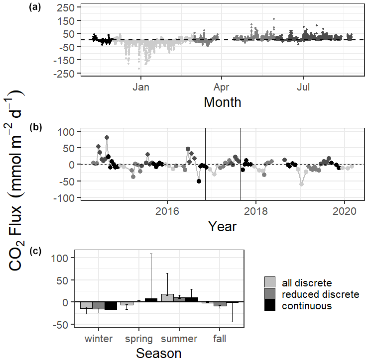
Figure 3CO2 flux calculated over the sampling periods from continuous (a) and discrete (b) data. Gray scale in (a) and (b) denote different seasons. Vertical lines in (b) denote the time period of continuous monitoring. (c) shows the seasonal mean CO2 flux. Error bars represent mean CO2 flux using Ho (2006) and Raymond and Cole (2001) wind speed parameterizations.
Results of the LDA incorporated carbonate system parameters along with additional environmental parameters to get a full picture of system variability over seasonal timescales (Table 1). The most important parameter in system variability that allowed differentiation between seasons was temperature (Table 1, Seasonal LD1), as would be expected with the clear seasonal temperature fluctuations (Fig. S1e). The second most important parameter for seasonal differentiation was chlorophyll, likely indicating clear seasonal phytoplankton blooms. The carbonate chemistry also played a critical role in seasonal differentiation, as pCO2 was the third most important factor (Table 1).
Table 1Coefficients of linear discriminants (LD) from LDA using continuous sensor data and other environmental parameters. Discriminants for both diel and seasonal variability shown.

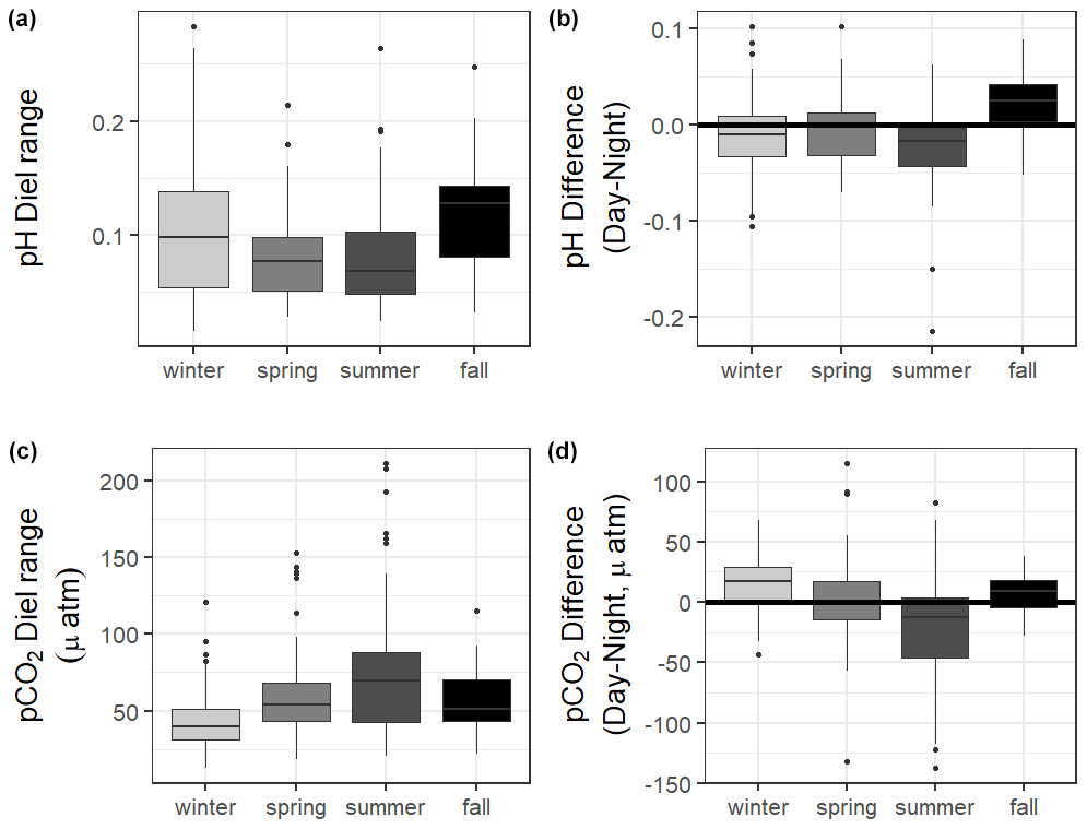
Figure 4Boxplots of the diel range (maximum minus minimum) and difference in daily parameter mean daytime minus nighttime measurements for pH and pCO2 from continuous sensor data.
3.2 Diel variability
The 10 months of in situ continuous monitoring revealed that there was substantial diel variability in measured parameters (Fig. 4, Table S3). Temperature had a mean diel range of 1.3 ± 0.8 ∘C (Table S3). Daytime and nighttime temperature differed significantly during the summer and fall months, with higher temperatures at night for both seasons (Table S3). The mean diel range of salinity was 3.4 ± 2.7 (Table S3). Daytime and nighttime salinity differed significantly during the winter and fall months, with higher salinities at night for both seasons. The mean diel range of pH was 0.09 ± 0.05 (Table S3). Daytime and nighttime pH differed significantly during the winter, summer, and fall, with nighttime pH significantly higher during summer and winter and lower during fall (Fig. 4, Table S3). The mean diel range of pCO2 was 58 ± 33 µatm (Fig. 4, Table S3). Daytime and nighttime pCO2 differed significantly during the winter and summer months, with nighttime pCO2 significantly higher during the summer and lower during the winter (Fig. 4, Table S3). No significant difference in daytime and nighttime DO were observed during any season (Fig. 5F; paired t-tests, winter p=0.1573, spring p=0.4877, summer p=0.794).
Loess models that investigated the evolution of day-night difference in parameters revealed that other environmental parameters, including salinity, temperature, and tide level, also had diel patterns that varied over the duration of our continuous monitoring (Fig. 5).
CO2 flux also fluctuated on a daily scale, with a mean diel range of 34.1 ± 29.0 mmol m−2 d−1 (Table S3). However, there was not a significant difference in CO2 flux of daytime versus nighttime hours for the entire monitoring period or any individual season based on α=0.05 (paired t-test, Table S3).
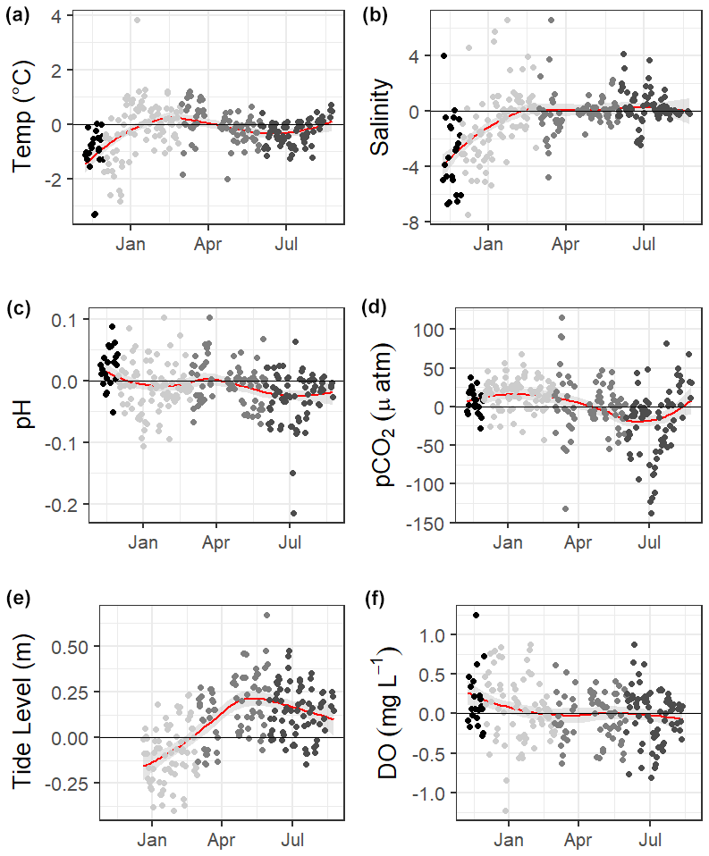
Figure 5Loess models (red line) and their confidence intervals (gray bands) showing the difference in daily daytime mean minus nighttime mean measurements. The gray scale of the data points represents the four seasons over which data were collected. Data span from 8 November 2016 to 3 August 2017, except for the tide data, which began 20 December 2016.
Results of the LDA for differentiation between daytime and nighttime conditions revealed that the most important factor was PAR, as would be expected (Table 1, Diel LD1). Temperature was the second most important factor to differentiate between day and night. The carbonate chemistry also played a critical role in day/night differentiation, as pCO2 was the third most important parameter, providing more evidence for differentiation between day and night than other parameters that would be expected to vary on a diel timescale (e.g., chlorophyll and DO) (Table 1).
3.3 Controlling factors and correlates
The relative influence of thermal and nonthermal factors () in controlling pCO2 varied over different timescales (Fig. 6, Table S4). Based on continuous data, nonthermal processes generally exerted more control than thermal processes () over the entire 5+ years of discrete monitoring, within each season, and over most () d (Fig. 6, Table S4). Annual from discrete data ranged from 0.50 to 1.16, with only one of the five sampled years having greater than one (i.e., more thermal influence; Table S4). While most individual seasons that were sampled experienced stronger nonthermal control on pCO2 (), the only season that never experienced stronger thermal control was summer, with summer values ranging from 0.21–0.35 for the 6 sampled years (Table S4).
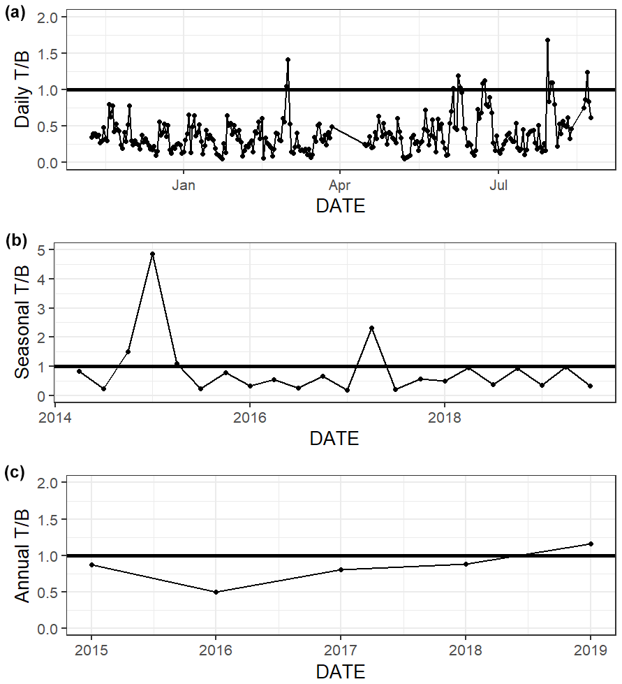
Figure 6Thermal versus nonthermal control on pCO2 daily (a), seasonal (b), and annual (c) timescales using both continuous sensor data (daily, from 8 November 2016 to 3 August 2017) and discrete sample data (seasonal and annual, from 2 May 2014–25 February 2020).
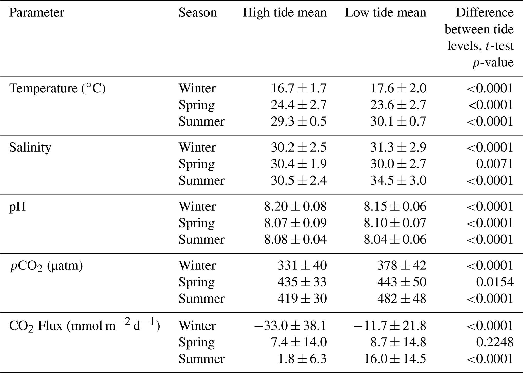
Tidal fluctuations seemed to have a significant effect on carbonate system parameters (Table 2). Both temperature and salinity were higher at low tide during the winter and summer months and higher at high tide during the spring. pCO2 was higher during low tide during all seasons. pH was higher during high tide during the winter and summer, but this reversed during the spring, when pH was higher at low tide. CO2 flux also varied with tidal fluctuations. CO2 flux was higher (more positive or less negative) in the low tide condition for all seasons (though the difference was not significant in spring), i.e., the location was less of a CO2 sink during low tide conditions in the winter and more of a CO2 source during low tide conditions in the summer.
Table 2Mean and standard deviation of temperature, salinity, pH, pCO2, and calculated CO2 flux (from continuous sensor measurements) during high and low tide conditions.
Mean water level varied between all seasons; mean spring (highest) water levels were on average 0.08 m higher than winter (lowest) water levels (ANOVA p<0.0001, fall was not considered because of a lack of water level data). The mean daily tidal range during our continuous monitoring period was 0.39 m ± 0.13 m, which did not significantly differ between seasons (ANOVA p=0.739). However, the day-night difference in tide level exhibited a strong seasonality, with spring and summer having higher tide levels during the daytime and winter having higher tide levels during the nighttime (Fig. 5).
There were significant correlations between carbonate system parameters (pH and pCO2) and many of the other environmental parameters, including wind speed, DO, turbidity, and fluorescent chlorophyll (Fig. 7, Table S5). Both the continuous and discrete sampling types indicate that pH has a significant negative relationship to both temperature and salinity and pCO2 has a significant positive relationship to both temperature and salinity (Fig. 7). However, correlations with temperature were stronger for continuous data and correlations with salinity were stronger for discrete data (Table S5). The strongest correlations between continuous carbonate system data and all investigated environmental parameters were with DO (positive correlation with pH and negative correlation with pCO2; Table S5). It is worth noting that there were no observations of hypoxia at our study site during our monitoring, with minimum DO levels of 3.9 and 4.0 mg L−1 for our continuous monitoring period and our discrete sampling period, respectively.
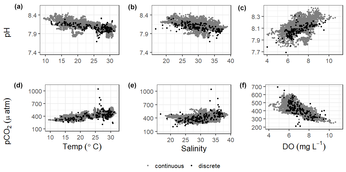
Figure 7Correlations of pH and pCO2 with temperature, salinity, and DO from continuous sensor data (gray) and all discrete data (black).
4.1 Comparing continuous monitoring and discrete sampling: representative sampling in a temporally variable environment
Discrete water sample collection and analysis is the most common method that has been employed to attempt to understand the carbonate system of estuaries. However, it is difficult to know if these samples are representative of the spatial and temporal variability in carbonate system parameters. While this time series study cannot conclude whether our broader sampling efforts in the MAE are representative of the spatial variability in the estuary, it can investigate how representative our bimonthly to monthly sampling is of the more high-frequency temporal variability that ASC experiences.
There were several instances where seasonal parameter means significantly differed between the 10-month continuous monitoring period and the 5+ year discrete sampling period (Table S2, C≠D or DC≠D) including temperature in the summer and fall, salinity in the spring, pH in the summer and fall, and pCO2 in winter, spring, and summer. While clear seasonal variability was demonstrated for most parameters (using both continuous and discrete data for the entire period), these differences between the 10-month continuous monitoring period and our 5+ year monitoring period illustrate that there is also interannual variability in the system. Therefore, short periods of monitoring are unable to fully capture current baseline conditions.
During the continuous monitoring period (2016–2017), we found no significant difference between sampling methods in the seasonal mean temperature, salinity, or pCO2. The two sampling methods also resulted in the same mean pH for all seasons except for summer, when the sensor data recorded a higher mean pH than discrete samples (Tables S1 and S2). During this case, we can conclude that discrete monitoring did not accurately represent the system variability that was able to be captured by the sensor monitoring. However, given that most seasons did not show differences in pH or pCO2 between sampling methods, the descriptive statistics associated with the discrete monitoring did a fair job of representing system means. This is evidence that long-term discrete monitoring efforts, which are much more widespread in estuarine systems than sensor deployments, can be generally representative of the system despite known temporal variability on shorter timescales. However, further study would be needed to determine if this applies throughout the system, as the upper estuary generally experiences greater variability.
Understanding the relationships of pH and pCO2 to temperature and salinity is important in a system (Fig. 7). Based on the results of an Analysis of Covariance (ANCOVA), the relationship (slope) of pH to both temperature and salinity and of pCO2 to salinity were not significantly different between types of monitoring (considering the sensor deployment period only), supporting the effectiveness of long-term discrete monitoring programs when sensors are unable to be deployed. However, ANCOVA did reveal that the relationship of pCO2 to temperature is significantly different (method : temp p=0.0062) between monitoring methods.
The high temporal resolution of sensor data is presumably better for estimating CO2 flux at a given location than discrete sampling. Previous studies have pointed out that discrete sampling methods, which generally involve only daytime sampling, do not adequately capture the diel variability in the carbonate system and may therefore lead to biased CO2 fluxes (Crosswell et al., 2017; Liu et al., 2016). However, we found no significant difference (within any season) between CO2 flux values calculated with hourly sensor data versus single, discrete samples collected monthly to twice monthly (Table S2, Fig. 3). Calculated CO2 fluxes also did not significantly differ between day and night during any season, despite some differences in pCO2 (Table S3), likely due to the large error associated with the calculation of CO2 flux (Table S1, Fig. 3) which will be further discussed below. Therefore, the expected underestimation of CO2 flux based on diel variability of pCO2 was not encountered at our study site, validating the use of discrete samples for quantification of CO2 fluxes (until methods with less associated error are available). Even given less error in calculated flux, estimated fluxes would likely not differ between methods on an annual scale (as pCO2 did not), but CO2 fluxes may differ on a seasonal scale since the differences between daytime and nighttime pCO2 were not consistent across seasons (Table S3, Fig. 4).
There are many factors contributing to error associated with CO2 flux. There is still large error associated with estimates of estuarine CO2 flux because turbulent mixing is difficult to model and turbulence is the main control on CO2 gas transfer velocity, k, in shallow water environments. Thus, our wind speed parameterization of k is imperfect and likely the greatest source of error (Borges and Abril, 2011; Van Dam et al., 2019). Other notable sources of error include the data treatment. For example, we chose to seasonally weight the individual calculated flux values in the calculation of annual flux to account for differences in sampling frequency between seasons. From continuous data, the weighted average flux was 0.2 mmol m−2 d−1, although choosing not to seasonally weight and simply look at the arithmetic mean of fluxes calculated directly from sampling dates would have resulted in an annual CO2 flux of −0.7 mmol m−2 d−1 for the same period. Similarly, the weighted average flux from all 5+ years of discrete data was −0.9 mmol m−2 d−1, but the arithmetic mean of fluxes would have resulted in an annual CO2 flux of 0.2 mmol m−2 d−1 for the same period. Another source of error that could be associated with the calculation of flux from the discrete data is the way in which wind speed data are aggregated to be used in the wind speed parameterization. We decided to use daily averages of the wind speed for calculations. Using the wind speed measured for the closest time to our sampling time or the monthly averaged wind speed may have resulted in very different flux values.
4.2 Factors controlling temporal variability in carbonate system parameters
Our study site had a relatively small range of pH and pCO2 on both diel and seasonal scales compared to other coastal regions (Challener et al., 2016; Yates et al., 2007). This small variability is likely tied to a combination of the subtropical setting (small temperature variability), the lower estuary position of our monitoring (further removed from the already small freshwater influence), little ocean upwelling influence, and the system's relatively high buffer capacity that results from the high alkalinity of the freshwater endmembers (Yao et al., 2020). Just as the extent of hypoxia-induced acidification was relatively low in Corpus Christi Bay because of the bay's high buffer capacity (McCutcheon et al., 2019), the extent of pH fluctuation resulting from all controlling factors at ASC would also be modulated by the region's high intrinsic buffer capacity.
4.2.1 Thermal and biological controls on carbonate chemistry
We demonstrated that both temperature and nonthermal processes exert control on pCO2, but nonthermal control generally surpasses thermal control in ASC over multiple timescales (Fig. 6, Table S4, ). The magnitude of pCO2 variation attributed to nonthermal processes varied greatly (i.e., ΔpCO2,nt had large standard deviations, Table S4). For example, during the year of strongest nonthermal control (2016), ΔpCO2,nt was 534 µatm versus ΔpCO2,nt of 209 µatm in the year of weakest thermal control (2019). Conversely, the magnitude of pCO2 variation attributed to temperature was consistent across timescales. For example, during the year of strongest thermal control (2015), ΔpCO2,t was 276 µatm versus ΔpCO2,t of 242 µatm in the year of weakest thermal control (2017). Spring and fall seasons, which experienced the greatest temperature swings (Table S1), had greater relative temperature control exerted on pCO2 out of all seasons (Fig. 6, Table S4). The difference in between sampling methods is relatively small over the 10-month sensor deployment period, but it is worth noting that did not align over shorter seasonal timescales sampling methods (Fig. 6, Table S4). Continuous monitoring demonstrated a greater magnitude of fluctuation resulting from both temperature and nonthermal processes (i.e., greater ΔpCO2,t and ΔpCO2,nt), indicating that the extremes are generally not captured by discrete, daytime sampling, and sensor data would provide a better understanding of system controls.
The greater influence of nonthermal controls that we report conflicts with Yao and Hu (2017), who found that ASC was primarily thermally controlled ( 1.53–1.79) from May 2014 to April 2015. Yao and Hu (2017) also found that locations in the upper estuary experienced lower during flooding conditions than drought conditions. Although the opposite was found at ASC, it is likely that the high calculated at ASC by Yao and Hu (2017) was still a result of the drought condition due to the long residence time of the estuary. Since 2015, there has not been another significant drought in the system, so it seems that nonthermal controls on pCO2 are more important at this location under normal freshwater inflow conditions.
Significantly warmer water temperatures were observed during the nighttime in both summer and fall (Fig. 5), indicating that temperature could exert a slight control on the carbonate system over a diel timescale. We note that significant differences in day and night temperature within seasons do not indicate that diel differences were observed on all days within the season, as large standard deviations in both daytime and nighttime values result in considerable overlap. More substantial temperature swings between seasons would result in more temperature control over a seasonal timescale. ASC seems to have less thermal control of the carbonate system than offshore GOM waters, as temperature had substantially higher explanatory value for pH and pCO2 based on simple linear regressions in offshore GOM waters (R2=0.81 and 0.78, respectively, Hu et al., 2018) than at ASC (R2=0.30 and 0.52, respectively, for sensor data and R2=0.38 and 0.25, respectively, for discrete data).
Though annual average pCO2 (and CO2 flux) are higher in the upper MAE and lower offshore than at our study site, the same seasonal patterns that we observed (i.e., elevated pCO2 and positive CO2 flux in the summer and depressed pCO2 and negative CO2 flux during the winter, Table S1, Fig. S1) has also been observed throughout the entire MAE and the open Gulf of Mexico (Hu et al., 2018; Yao and Hu, 2017). These seasonal patterns correspond with both the directional response of the system to temperature and the net community metabolism response to changing temperature, i.e., elevated respiration in the summer months (Caffrey, 2004). Despite there being no observations of hypoxia, there was a strong relationship between the carbonate system parameters and DO (Fig. 7, Table S5), suggesting that net ecosystem metabolism may exert an important control on the carbonate system on seasonal timescales. The lack of day-night difference in DO (Fig. 5f) despite the significant day-night difference in both pH and pCO2 suggests that net community metabolism is likely not a strong controlling factor on diel timescales. Biological control likely becomes more important over seasonal timescales.
4.2.2 Tidal control on carbonate chemistry
While the tidal range in the northwestern GOM is relatively small (1.30 m over our 10-month continuous monitoring period), the tidal inlet location of our study site results in proportionally more “coastal water” during high tide and proportionally more “estuarine water” during low tide. The carbonate chemistry signal of these different water masses was seen in the differences between high tide and low tide conditions at ASC (i.e., high tide having lower pCO2 because coastal waters are less heterotrophic than estuarine waters, Table 2). Consequently, the relative importance of thermal versus nonthermal controls may be modulated by tide level. We calculated the thermal and nonthermal pCO2 terms separately during high tide and low tide periods and found that nonthermal control is more important during low tide conditions (within each season is 0.10 ± 0.07 lower during the low tide than high tide). This is likely because low tide has proportionally more “estuarine water” at the location and because there is less volume of water for the end products of biological processes to accumulate. The difference in between high tide and low tide conditions was greatest in the spring, likely due to a combination of elevated spring-time productivity and larger tidal ranges in the spring.
The GOM is one of the few places in the world that experiences diurnal tides (Seim et al., 1987; Thurman, 1994), so theoretically, the fluctuations in pCO2 associated with tides may align to either amplify or reduce/reverse the fluctuations that would result from diel variability in net community metabolism. Based on diel tidal fluctuations at this site (i.e., higher tides during the day in the spring and summer and higher tides at night during the winter, Fig. 5e) and the higher pCO2 associated with low tide (Table 2), tidal control should amplify the biological signal (nighttime pCO2> daytime pCO2) during spring and summer and reduce or reverse the biological signal during the winter. This tidal control can explain the diel variability present in our pCO2 data, which showed the full reversal of the expected biological signal in the winter (Fig. 5c, Table S3, nighttime pCO2< daytime pCO2), i.e., the higher nighttime tides in winter brought in enough low CO2 water from offshore to fully offset any nighttime buildup of CO2 from the lack of photosynthesis. However, we note that the expected diel, biological control was likely minimal since daytime DO was not consistently higher than nighttime DO (Fig. 5f). The same seasonal pattern diel tide fluctuations were exhibited from 20 December 2016 (when the tide data is first available) through the rest of our discrete monitoring period (25 February 2020), indicating that tidal control on diel variability of carbonate system parameters was likely consistent throughout this 3+ year period. The diel variability in pH did not mirror pCO2 as would be expected (Fig. 5). The relationship between pH and tide level more closely mirrored the relationships of salinity and temperature to tide level (versus pCO2 relationship to tide level; Table 2), indicating that controlling factors of the carbonate system may not be exerted equally on both pH and pCO2 over different timescales.
4.2.3 Salinity and freshwater inflow controls on carbonate chemistry
Previous studies have indicated that freshwater inflow may exert a primary control on the carbonate system in the estuaries of the northwestern GOM (Hu et al., 2015; Yao et al., 2020; Yao and Hu, 2017). Though the river water still has elevated pCO2 and depressed pH compared to the seawater endmember, the high riverine alkalinity (often higher than the seawater endmember) in the region results in relatively well-buffered estuarine conditions in MAE (Yao and Hu, 2017). Carbonate system variability is much lower at ASC than it is in the more upper reaches of MAE, likely due to the lesser influence of freshwater inflow and its associated changes in biological activity at ASC (Yao and Hu, 2017). Given the location of our sampling in the lower portion of the estuary and the long residence time in the system, we did not directly address river discharge as a controlling factor, but the influence of freshwater inflow may be evident in the response of the system to changes in salinity. Fluctuating salinity at ASC may also result from direct precipitation, stratification, and tidal fluctuations; however, the low R2 (0.02) associated with a simple linear regression between tide level and salinity (p<0.0001) indicates that salinity fluctuations are more indicative of nontidal factors. Salinity data from both sensor and discrete monitoring were strongly correlated with both pH and pCO2, with correlation coefficients nearing (continuous) or surpassing (discrete) that of the correlations with temperature (Fig. 7; Table S5). Periods of lower salinity had higher pH and lower pCO2, likely due to enhanced freshwater influence and subsequent elevated primary productivity at the study site.
4.2.4 Wind speed and CO2 inventory
We investigated wind speed as a possible control on the carbonate system to gain insight into the effect of wind-driven CO2 fluxes on the inventory of CO2 in the water column (and subsequent impacts to the entire carbonate system). The Texas coast has relatively high wind speeds, with the mean wind speed observed during our continuous monitoring period being 5.8 m s−1. While this results in relatively high calculated CO2 fluxes (Fig. 3), the seasonal relationship between pCO2 and wind speed does not support a change in inventory with higher winds. Since spring and summer both have a mean estuarine pCO2 greater than atmospheric levels (and positive CO2 flux, Table S1), a negative relationship between wind speed and pCO2 would be necessary to support this hypothesis, but winter, spring, and fall all experience increases in pCO2 with increasing wind based on simple linear regression.
4.3 Carbonate chemistry as a component of overall system variability
Estuaries and coastal areas are dynamic systems with human influence, riverine influence, and influence from an array of biogeochemical processes, resulting in highly variable environmental conditions. Based on a LDA used to assess overall system variability using a suite of environmental parameters compiled at a single location, we can conclude that carbonate chemistry parameters are among the most important of variants on both daily and seasonal timescales in this coastal setting. Of the two carbonate system components that we incorporated (pH and pCO2), pCO2 was the most critical in discriminating along diel or seasonal scales despite similar seasonal differences that were identified by ANOVA (Table S2) and more seasons with significant diel differences in pH (Table S3). pH seemed to be a larger component of overall system variability on a seasonal time scale (compared to the very small contribution seen on a diel scale, Table 1). Given that seasonal and diel variability in carbonate chemistry at this location is relatively small compared to other coastal areas that are in the literature, the high contribution of carbonate chemistry to the overall system variability that we detected is likely to be present at other coastal locations around the world.
We monitored carbonate chemistry parameters (pH and pCO2) using both sensor deployments (10 months) and discrete sample collection (5+ years) at the Aransas Ship Channel, TX, to characterize temporal variability. Significant seasonal variability and diel variability in carbonate system parameters were both present at the location. Diel fluctuations were smaller than many other areas previously studied. The difference between daytime and nighttime values of carbonate system parameters varied between seasons, occasionally reversing the expected diel variability due to biological processes. Tide level (despite the small tidal range), temperature, freshwater influence, and biological activity all seem to exert important controls on the carbonate system at the location. The relative importance of the different controls varied with timescale, and controls were not always exerted equally on both pH and pCO2. Carbonate chemistry (particularly pCO2) was among the most important environmental parameters of overall system variability for distinguishing between both diel and seasonal environmental conditions.
Despite known temporal variability on shorter timescales, discrete sampling was generally representative of the average carbonate system on a seasonal and annual basis based on comparison with our sensor data. Discrete data captured interannual variability, which could not be captured by shorter-term continuous sensor data. Additionally, there was no difference in CO2 flux between sampling types. All of these findings support the validity of discrete sample collection for carbonate system characterization at this location.
This is one of the first studies investigating high-temporal frequency data from deployed sensors that measure carbonate system parameters in an estuary-influenced environment. Long-term, effective deployments of these monitoring tools could greatly improve our understanding of estuarine systems. This study's detailed investigation of data from multiple, co-located environmental sensors was able to provide insight into potential driving forces of carbonate chemistry on diel and seasonal timescales; this provides strong support for the implementation of carbonate chemistry monitoring in conjunction with preexisting coastal environmental monitoring infrastructure. Strategically locating such sensors in areas that are subject to local acidification drivers or support large biodiversity or commercially important species may be the most crucial in guiding future mitigation and adaptation strategies for natural systems and aquaculture facilities.
Continuous sensor data are archived with the National Oceanic and Atmospheric Administration's (NOAA's) National Centers for Environmental Information (NCEI) (https://doi.org/10.25921/dkg3-1989, Hu and McCutcheon, 2020). Discrete sample data are available in two separate datasets archived with National Science Foundation's Biological and Chemical Oceanography Data Management Office (BCO-DMO) (https://doi.org/10.1575/1912/bco-dmo.784673.1, Hu, 2019) and https://doi.org/10.26008/1912/bco-dmo.835227.1 (McCutcheon and Hu, 2021).
The supplement related to this article is available online at: https://doi.org/10.5194/bg-18-4571-2021-supplement.
MRM and XH defined the scope of this work. XH received funding for all components of the work. MRM, HY, and CJS performed field sampling and laboratory analysis of samples. MRM prepared the initial manuscript and all co-authors contributed to revisions.
The authors declare that they have no conflict of interest.
Publisher's note: Copernicus Publications remains neutral with regard to jurisdictional claims in published maps and institutional affiliations.
Thanks to Rae Mooney from Coastal Bend Bays and Estuaries Program for assistance in the initial sensor setup. We also appreciate the support from the Mission-Aransas National Estuarine Research Reserve in allowing us the boat-of-opportunity for our ongoing discrete sample collections and the University of Texas Marine Science Institute for allowing us access to their research pier for sensor deployment. A special thanks to Hongjie Wang, Lisette Alcocer, Allen Dees, and Karen Alvarado for assistance with field work. We would also like to thank Melissa Ward, our other anonymous referee, and the Associate Editor, Tyler Cyronak, for aiding in the considerable improvement of this manuscript.
This research has been supported by the National Science Foundation (grant no. OCE-1654232), the National Oceanic and Atmospheric Administration (grant no. NA15NOS4780185), and the United States Environmental Protection Agency's National Estuary Program via the Coastal Bend Bays and Estuaries Program (contract no. 1605).
This paper was edited by Tyler Cyronak and reviewed by Melissa Ward and one anonymous referee.
Abril, G., Commarieu, M. V., Sottolichio, A., Bretel, P., and Guérin, F.: Turbidity limits gas exchange in a large macrotidal estuary, Estuar. Coast. Shelf Sci., 83, 342–348, https://doi.org/10.1016/j.ecss.2009.03.006, 2009.
Andersson, A., Falck, E., Sjöblom, A., Kljun, N., Sahlée, E., Omar, A. M., and Rutgersson, A.: Air‐sea gas transfer in high Arctic fjords, Geophys. Res. Lett., 44, 2519–2526, https://doi.org/10.1002/2016GL072373, 2017.
Barton, A., Waldbusser, G. G., Feely, R. A., Weisberg, S. B., Newton, J. A., Hales, B., Cudd, S., Eudeline, B., Langdon, C. J., Jefferds, I., King, T., Suhrbier, A., and Mclaughlin, K.: Impacts of coastal acidification on the pacific northwest shellfish industry and adaptation strategies implemented in response, Oceanography, 28, 146–159, 2015.
Bednaršek, N., Tarling, G. A., Bakker, D. C. E., Fielding, S., Jones, E. M., Venables, H. J., Ward, P., Kuzirian, A., Lézé, B., Feely, R. A., and Murphy, E. J.: Extensive dissolution of live pteropods in the Southern Ocean, Nat. Geosci., 5, 881–885, https://doi.org/10.1038/ngeo1635, 2012.
Borges, A. V.: Do we have enough pieces of the jigsaw to integrate CO2 fluxes in the coastal ocean?, Estuaries, 28, 3–27, 2005.
Borges, A. V. and Abril, G.: Carbon Dioxide and Methane Dynamics in Estuaries, in: Treatise on Estuarine and Coastal Science, edited by: Wolanski, E. and McLusky, D., Academic Press, 119–161, https://doi.org/10.1016/B978-0-12-374711-2.00504-0, 2011.
Bresnahan, P. J., Martz, T. R., Takeshita, Y., Johnson, K. S., and LaShomb, M.: Best practices for autonomous measurement of seawater pH with the Honeywell Durafet, Method. Oceanogr., 9, 44–60, https://doi.org/10.1016/j.mio.2014.08.003, 2014.
Caffrey, J. M.: Factors controlling net ecosystem metabolism in U.S. estuaries, Estuaries 27, 90–101, https://doi.org/10.1007/BF02803563, 2004.
Cai, W.-J.: Estuarine and Coastal Ocean Carbon Paradox: CO2 Sinks or Sites of Terrestrial Carbon Incineration?, Ann. Rev. Mar. Sci., 3, 123–145, https://doi.org/10.1146/annurev-marine-120709-142723, 2011.
Cai, W.-J., Hu, X., Huang, W.-J., Murrell, M. C., Lehrter, J. C., Lohrenz, S. E., Chou, W.-C., Zhai, W., Hollibaugh, J. T., Wang, Y., Zhao, P., Guo, X., Gundersen, K., Dai, M., and Gong, G.-C.: Acidification of subsurface coastal waters enhanced by eutrophication, Nat. Geosci., 4, 766–770, https://doi.org/10.1038/ngeo1297, 2011.
Carter, B. R., Radich, J. A., Doyle, H. L., and Dickson, A. G.: An automatic system for spectrophotometric seawater pH measurements, Limnol. Oceanogr.-Method., 11, 16–27, 2013.
Challener, R. C., Robbins, L. L., and McClintock, J. B.: Variability of the carbonate chemistry in a shallow, seagrass-dominated ecosystem: Implications for ocean acidification experiments, Mar. Freshw. Res., 67, 163–172, https://doi.org/10.1071/MF14219, 2016.
Crosswell, J. R., Anderson, I. C., Stanhope, J. W., Van Dam, B., Brush, M. J., Ensign, S., Piehler, M. F., McKee, B., Bost, M., and Paerl, H. W.: Carbon budget of a shallow, lagoonal estuary: Transformations and source-sink dynamics along the river-estuary-ocean continuum, Limnol. Oceanogr., 62, S29–S45, https://doi.org/10.1002/lno.10631, 2017.
Cyronak, T., Andersson, A. J., D'Angelo, S., Bresnahan, P., Davidson, C., Griffin, A., Kindeberg, T., Pennise, J., Takeshita, Y., and White, M.: Short-term spatial and temporal carbonate chemistry variability in two contrasting seagrass meadows: Implications for pH buffering capacities, Estuar. Coast., 41, 1282–1296, https://doi.org/10.1007/s12237-017-0356-5, 2018.
Dickson, A. G.: Standard potential of the reaction: AgCl(s) + 1 2H2(g) = Ag(s) + HCl(aq), and and the standard acidity constant of the ion HSO in synthetic sea water from 273.15 to 318.15 K, J. Chem. Thermodyn,. 22, 113–127, https://doi.org/10.1016/0021-9614(90)90074-Z, 1990.
Douglas, N. K. and Byrne, R. H.: Spectrophotometric pH measurements from river to sea: Calibration of mCP for and K, Mar. Chem., 197, 64–69, 2017.
Ekstrom, J. A., Suatoni, L., Cooley, S. R., Pendleton, L. H., Waldbusser, G. G., Cinner, J. E., Ritter, J., Langdon, C., van Hooidonk, R., Gledhill, D., Wellman, K., Beck, M. W., Brander, L. M., Rittschof, D., Doherty, C., Edwards, P. E. T., and Portela, R.: Vulnerability and adaptation of US shellfisheries to ocean acidification, Nat. Clim. Change, 5, 207–214, https://doi.org/10.1038/nclimate2508, 2015.
Gazeau, F., Quiblier, C., Jansen, J.M., Gattuso, J.-P., Middelburg, J. J., and Heip, C. H. R.: Impact of elevated CO2 on shellfish calcification, Geophys. Res. Lett., 34, L07603, https://doi.org/10.1029/2006GL028554, 2007.
Gobler, C. J. and Talmage, S. C.: Physiological response and resilience of early life-stage Eastern oysters (Crassostrea virginica) to past, present and future ocean acidification, Conserv. Physiol., 2, 1–15, 2014.
Ho, D. T., Law, C. S., Smith, M. J., Schlosser, P., Harvey, M., and Hill, P.: Measurements of air-sea gas exchange at high wind speeds in the Southern Ocean: Implications for global parameterizations, Geophys. Res. Lett., 33, 1–6, https://doi.org/10.1029/2006GL026817, 2006.
Hofmann, G. E., Smith, J. E., Johnson, K. S., Send, U., Levin, L. A., Micheli, F., Paytan, A., Price, N. N., Peterson, B., Takeshita, Y., Matson, P. G., Crook, E. D., Kroeker, K. J., Gambi, M. C., Rivest, E. B., Frieder, C. A., Yu, P. C., and Martz, T. R.: High-frequency dynamics of ocean pH: a multi-ecosystem comparison, PLoS One, 6, e28983, https://doi.org/10.1371/journal.pone.0028983, 2011.
Hsu, S. A.: Determining the power-law wind-profile exponent under near-neutral stability conditions at sea, J. Appl. Meteorol., 33, 757–765, 1994.
Hu, X.: Carbonate chemistry effects from Hurricane Harvey in San Antonio Bay and Mission Aransas Estuary from 2017-02-22 to 2018-11-15, Biological and Chemical Oceanography Data Management Office (BCO-DMO), (Version 1) Version Date 2019-12-19 [data set], https://doi.org/10.1575/1912/bco-dmo.784673.1, last access: 19 December 2019.
Hu, X., Beseres Pollack, J., McCutcheon, M. R., Montagna, P. A., and Ouyang, Z.: Long-term alkalinity decrease and acidification of estuaries in Northwestern Gulf of Mexico, Environ. Sci. Technol., 49, 3401–3409, https://doi.org/10.1021/es505945p, 2015.
Hu, X., Nuttall, M. F., Wang, H., Yao, H., Staryk, C. J., McCutcheon, M. R., Eckert, R. J., Embesi, J. A., Johnston, M. A., Hickerson, E. L., Schmahl, G. P., Manzello, D., Enochs, I. C., DiMarco, S., and Barbero, L.: Seasonal variability of carbonate chemistry and decadal changes in waters of a marine sanctuary in the Northwestern Gulf of Mexico, Mar. Chem., 205, 16–28, https://doi.org/10.1016/j.marchem.2018.07.006, 2018.
Hu, X. and McCutcheon, M. R.: Sensor continuous measurements of pH, partial pressure of carbon dioxide (pCO2), salinity and temperature at the University of Texas Marine Science Institute Research Pier, Aransas Ship Channel, TX, Gulf of Mexico from 2016-11-08 to 2017-08-23 (NCEI Accession 0222572), NOAA National Centers for Environmental Information [data set], https://doi.org/10.25921/dkg3-1989, last access: 5 December 2020.
Jiang, L.-Q., Cai, W.-J., and Wang, Y.: A comparative study of carbon dioxide degassing in river- and marine-dominated estuaries, Limnol. Oceanogr., 53, 2603–2615, https://doi.org/10.4319/lo.2008.53.6.2603, 2008.
Jiang, L. Q., Cai, W. J., Wang, Y., and Bauer, J. E.: Influence of terrestrial inputs on continental shelf carbon dioxide, Biogeosciences 10, 839–849, https://doi.org/10.5194/bg-10-839-2013, 2013.
Kealoha, A. K., Shamberger, K. E. F., DiMarco, S. F., Thyng, K. M., Hetland, R. D., Manzello, D. P., Slowey, N. C., and Enochs, I. C.: Surface water CO2 variability in the Gulf of Mexico (1996–2017), Sci. Rep., 10, 1–13, https://doi.org/10.1038/s41598-020-68924-0, 2020.
Laruelle, G. G., Cai, W.-J., Hu, X., Gruber, N., Mackenzie, F. T., and Regnier, P.: Continental shelves as a variable but increasing global sink for atmospheric carbon dioxide, Nat. Commun., 9, 454, https://doi.org/10.1038/s41467-017-02738-z, 2018.
Li, D., Chen, J., Ni, X., Wang, K., Zeng, D., Wang, B., Jin, H., Huang, D., and Cai, W. J.: Effects of biological production and vertical mixing on sea surface pCO2 variations in the Changjiang River Plume during early autumn: A buoy-based time series study, J. Geophys. Res.-Ocean., 123, 6156–6173, https://doi.org/10.1029/2017JC013740, 2018.
Liu, H., Zhang, Q., Katul, G. G., Cole, J. J., Chapin, F. S., and MacIntyre, S.: Large CO2 effluxes at night and during synoptic weather events significantly contribute to CO2 emissions from a reservoir, Environ. Res. Lett., 11, 1–8, https://doi.org/10.1088/1748-9326/11/6/064001, 2016.
Mathis, J. T., Pickart, R. S., Byrne, R. H., Mcneil, C. L., Moore, G. W. K., Juranek, L. W., Liu, X., Ma, J., Easley, R. A., Elliot, M. M., Cross, J. N., Reisdorph, S. C., Bahr, F., Morison, J., Lichendorf, T., and Feely, R. A.: Storm-induced upwelling of high pCO2 waters onto the continental shelf of the western Arctic Ocean and implications for carbonate mineral saturation states, Geophys. Res. Lett., 39, 4–9, https://doi.org/10.1029/2012GL051574, 2012.
McCutcheon, M. R., Staryk, C. J., and Hu, X.: Characteristics of the carbonate system in a semiarid estuary that experiences summertime hypoxia, Estuar. Coast., 42, 1509–1523, https://doi.org/10.1007/s12237-019-00588-0, 2019.
McCutcheon, M. R. and Hu, X.: Carbonate chemistry in Mission Aransas Estuary from May 2014 to February 2017 and December 2018 to February 2020, Biological and Chemical Oceanography Data Management Office (BCO-DMO), (Version 1) Version Date 2021-01-04 [data set], https://doi.org/10.26008/1912/bco-dmo.835227.1, last access: 4 January 2021.
Millero, F. J.: Carbonate constant for estuarine waters, Mar. Freshw. Res., 61, 139–142, 2010.
Montagna, P. A., Brenner, J., Gibeaut, J., and Morehead, S.: chap. 4: Coastal Impacts, in: The Impact of Global Warming on Texas, edited by: Schmandt, J., Clarkson, J., and North, G. R., University of Texas Press, Austin, 96–123, 2011.
Raymond, P. A. and Cole, J. J.: Gas exchange in rivers and estuaries: Choosing a gas transfer velocity, Estuaries, 24, 312–317, https://doi.org/10.2307/1352954 2001.
Robbins, L. L. and Lisle, J. T.: Regional acidification trends in florida shellfish estuaries: a 20+ year look at pH, oxygen, temperature, and salinity, Estuar. Coast., 41, 1268–1281, https://doi.org/10.1007/s12237-017-0353-8, 2018.
Sastri, A. R., Christian, J. R., Achterberg, E. P., Atamanchuk, D., Buck, J. J. H., Bresnahan, P., Duke, P. J., Evans, W., Gonski, S. F., Johnson, B., Juniper, S. K., Mihaly, S., Miller, L. A., Morley, M., Murphy, D., Nakaoka, S. I., Ono, T., Parker, G., Simpson, K., and Tsunoda, T.: Perspectives on in situ sensors for ocean acidification research, Front. Mar. Sci., 6, 1–6, https://doi.org/10.3389/fmars.2019.00653, 2019.
Schulz, K. G. and Riebesell, U.: Diurnal changes in seawater carbonate chemistry speciation at increasing atmospheric carbon dioxide, Mar. Biol., 160, 1889–1899, https://doi.org/10.1007/s00227-012-1965-y, 2013.
Seim, H. E., Kjerfve, B., and Sneed, J. E.: Tides of Mississippi Sound and the adjacent continental shelf, Estuar. Coast. Shelf Sci., 25, 143–156, https://doi.org/10.1016/0272-7714(87)90118-1, 1987.
Semesi, I. S., Beer, S., and Björk, M.: Seagrass photosynthesis controls rates of calcification and photosynthesis of calcareous macroalgae in a tropical seagrass meadow, Mar. Ecol. Prog. Ser., 382, 41–47, https://doi.org/10.3354/meps07973, 2009.
Shadwick E. H., Friedrichs M. A. M., Najjar R.G., De Meo, O. A., Friedman, J. R., Da, F., and Reay, W. G.: High-Frequency CO2 System Variability Over the Winter-to-Spring Transition in a Coastal Plain Estuary, J Geophys. Res.-Ocean., 124, 7626–7642, https://doi.org/10.1029/2019JC015246, 2019.
Solis, R. S. and Powell, G. L.: Hydrography, Mixing Characteristics, and Residence Time of Gulf of Mexico Estuaries, in: Biogeochemistry of Gulf of Mexico Estuaries, edited by: Bianchi, T. S., Pennock, J. R., and Twilley, R. R., John Wiley & Sons, Inc: New York, 29–61, 1999.
Takahashi, T., Sutherland, S. C., Sweeney, C., Poisson, A., Metzl, N., Tilbrook, B., Bates, N., Wanninkhof, R., Feely, R. A., Sabine, C., Olafsson, J., and Nojiri, Y.: Global sea-air CO2 flux based on climatological surface ocean pCO2, and seasonal biological and temperature effects, Deep.-Sea Res. Pt. II, 49, 1601–1622, https://doi.org/10.1016/S0967-0645(02)00003-6, 2002.
Thurman, H. V.: Introductory Oceanography, 7th Edn., Indiana, USA, Prentice Hall, 252–276, 1994.
Uppström, L. R.: The boron/chlorinity ratio of deep-sea water from the Pacific Ocean, Deep-Sea Res. Oceanogr. Abstr., 21, 161–162, https://doi.org/10.1016/0011-7471(74)90074-6, 1974.
USGS: Discharge Between San Antonio Bay and Aransas Bay, Southern Gulf Coast, Texas, May–September 1999, 2001.
Van Dam, B. R., Edson, J. B., and Tobias, C.: Parameterizing Air-Water Gas Exchange in the Shallow, Microtidal New River Estuary, J. Geophys. Res.-Biogeo., 124, 2351–2363, https://doi.org/10.1029/2018JG004908, 2019.
Waldbusser, G. G. and Salisbury, J. E.: Ocean acidification in the coastal zone from an organism's perspective: multiple system parameters, frequency domains, and habitats, Ann. Rev. Mar. Sci., 6, 221–47, https://doi.org/10.1146/annurev-marine-121211-172238, 2014.
Wanninkhof, R.: Relationship between wind speed and gas exchange, J. Geophys. Res., 97, 7373–7382, https://doi.org/10.1029/92JC00188, 1992.
Wanninkhof, R., Asher, W. E., Ho, D. T., Sweeney, C., and McGillis, W. R.: Advances in quantifying air-sea gas exchange and environmental forcing, Ann. Rev. Mar. Sci., 1, 213–244, https://doi.org/10.1146/annurev.marine.010908.163742, 2009.
Weiss, R. F.: Carbon dioxide in water and seawater: the solubility of a non-ideal gas, Mar. Chem., 2, 203–215, 1974.
Westfall, P. H.: Multiple testing of general contrasts using logical constraints and correlations, J. Am. Stat. Assoc., 92, 299–306, https://doi.org/10.1080/01621459.1997.10473627, 1997.
Yao, H. and Hu, X.: Responses of carbonate system and CO2 flux to extended drought and intense flooding in a semiarid subtropical estuary, Limnol. Oceanogr., 62, S112–S130, https://doi.org/10.1002/lno.10646, 2017.
Yao, H., McCutcheon, M. R., Staryk, C. J., and Hu, X.: Hydrologic controls on CO2 chemistry and flux in subtropical lagoonal estuaries of the northwestern Gulf of Mexico, Limnol. Oceanogr., 65, 1380–1398, https://doi.org/10.1002/lno.11394, 2020.
Yates, K. K., Dufore, C., Smiley, N., Jackson, C., and Halley, R. B.: Diurnal variation of oxygen and carbonate system parameters in Tampa Bay and Florida Bay, Mar. Chem., 104, 110–124, https://doi.org/10.1016/j.marchem.2006.12.008, 2007.