the Creative Commons Attribution 4.0 License.
the Creative Commons Attribution 4.0 License.
 | 12 Aug 2021
Temporal dynamics of tree xylem water isotopes: in situ monitoring and modeling
Stefan Seeger
Markus Weiler
We developed a setup for a fully automated, high-frequency in situ monitoring system of the stable water isotope deuterium and 18O in soil water and tree xylem. The setup was tested for 12 weeks within an isotopic labeling experiment during a large artificial sprinkling experiment including three mature European beech (Fagus sylvatica) trees. Our setup allowed for one measurement every 12–20 min, enabling us to obtain about seven measurements per day for each of our 15 in situ probes in the soil and tree xylem. While the labeling induced an abrupt step pulse in the soil water isotopic signature, it took 7 to 10 d until the isotopic signatures at the trees' stem bases reached their peak label concentrations and it took about 14 d until the isotopic signatures at 8 m stem height leveled off around the same values. During the experiment, we observed the effects of several rain events and dry periods on the xylem water isotopic signatures, which fluctuated between the measured isotopic signatures observed in the upper and lower soil horizons. In order to explain our observations, we combined an already existing root water uptake (RWU) model with a newly developed approach to simulate the propagation of isotopic signatures from the root tips to the stem base and further up along the stem. The key to a proper simulation of the observed short-term dynamics of xylem water isotopes was accounting for sap flow velocities and the flow path length distribution within the root and stem xylem. Our modeling framework allowed us to identify parameter values that relate to root depth, horizontal root distribution and wilting point. The insights gained from this study can help to improve the representation of stable water isotopes in trees within ecohydrological models and the prediction of transit time distribution and water age of transpiration fluxes.
- Article
(11569 KB) - Full-text XML
-
Supplement
(2010 KB) - BibTeX
- EndNote


Transpiration from terrestrial plants is a key component of the global hydrological cycle, and its fraction of the total water balance might even increase under projected future climatic conditions (Bernacchi and VanLoocke, 2015). Process-based ecohydrological models can be an important tool to gain realistic estimates of the vegetation's response to climatic changes. Such process-based models need detailed data on plant water uptake and transpiration. These processes can and have been studied intensively with the help of stable water isotopes (White et al., 1985; Calder, 1991; Dawson and Ehleringer, 1991; Busch et al., 1992; Ehleringer and Dawson, 1992; Zhang et al., 1999; Dawson et al., 2002).
1.1 Isotope-tracer-enhanced observations of tree water dynamics
To observe the temporal dynamics of water within the soil–plant–atmosphere continuum (SPAC), isotopic labeling experiments offer a unique opportunity to create distinct pulses that can be traced from the soil, through the plant, to the atmosphere. For small experimental plots, chamber-based measurements can capture the isotopic composition of transpiration (δT) following isotopically labeled irrigation pulses (e.g., Yepez et al., 2005; Volkmann et al., 2016a). Due to dimensional limits set by the size of the required chamber, this method is not applicable to adult trees.
Larger-scale irrigation experiments were conducted in green house experiments with around 15 m high tropical trees (Evaristo et al., 2019) and in a central European forest with grown, 25 m high, specimens of Fagus sylvatica and Abies alba (Magh et al., 2020). Instead of chamber measurements of δT, they extracted water from tree crown branches to monitor the isotopic composition of xylem water (δxyl). For 7 months, Evaristo et al. (2019) had a weekly δxyl sampling scheme, while Magh et al. (2020) started with a sub-daily δxyl sampling scheme for 5 d and continued the following 2 months with a sampling frequency of 4 to 6 d. Both experiments observed notable delays (days to weeks) between tracer application and detection within the sampled crown branches.
A more specific investigation of tree water dynamics can be achieved by skipping soil and roots and directly injecting small amounts of D2O into the stem base (James et al., 2003; Meinzer et al., 2006; Schwendenmann et al., 2010; Gaines et al., 2016). Due to the high deuterium concentrations of the injected label, tracer breakthrough curves within the tree crown could be acquired by analyzing condensate from branch or foliar samples placed into zipper bags. Time delays between tracer application and maximum tracer concentrations within the tree crowns have mostly been reported to amount to a few days, but for a 50 m high specimen of Tsuga heterophylla Meinzer et al. (2006) also reported a delay of about 30 d. A comparison of heat-tracing-derived sap flux velocities with isotope-tracing-derived velocities revealed that the latter may be 4 to 16 times higher (Meinzer et al., 2006; Gaines et al., 2016).
1.2 Water uptake and tree isotope modeling
Rothfuss and Javaux (2017) have reviewed 159 studies combining root water uptake (RWU) and isotopes. A total of 46 % of those studies used isotopic data to infer a specific soil layer or water pool as a source of RWU. Another 50 % of those studies used two- or multi-source linear mixing models of varying statistical sophistication. Only the remaining 4 % of the reviewed studies used physically based analytical or numerical models. This means that the vast majority of isotope-based RWU studies are based on graphic or statistical methods, which allow a description of observations but abstain from offering physically based models, which could be used to predict the reaction of RWU to changing environmental conditions.
Lv (2014), Rabbel et al. (2018) and Brinkmann et al. (2018) have modeled RWU of trees with implementations of a Feddes-style RWU model described by Feddes et al. (1976) and Jarvis (1989) as implemented within the soil hydrological model HYDRUS-1D (Šimůnek et al., 2008). Even though the Feddes RWU model was originally developed to model water uptake of agricultural crops, the above-listed applications demonstrated that Feddes RWU models are also suited to simulate RWU of mature trees. Brinkmann et al. (2018) used a Feddes RWU model, driven with soil water potentials and soil 18O concentrations simulated with an isotope-enabled version of HYDRUS-1D (Stumpp et al., 2012), to compute δ18O signatures of RWU. These predictions compared well to fortnightly sampled δ18O values of branch xylem water.
The assumption that isotopic signatures of RWU (δRWU) are directly related to simultaneously sampled δxyl has been challenged by studies of Knighton et al. (2020) and De Deurwaerder et al. (2020). Knighton et al. (2020) juxtaposed a “zero storage case” (δRWU=δxyl) and two alternative cases (well mixed and piston flow) that included tree internal water storage. Model results for the cases with tree internal water storage compared better to observational data than the zero storage case. Due to a limited temporal resolution of their observed data, Knighton et al. (2020) were not able to conclude whether the piston flow or the well-mixed case was more appropriate and hypothesized that the actual behavior of the system may lie between those two cases. De Deurwaerder et al. (2020) proposed a model that comprised a soil-water-potential-driven RWU component and a stem water transport module that is based on an advection–diffusion model coupled to sap flow velocities. Based on their model, De Deurwaerder et al. (2020) predicted that diel fluctuations of δRWU (caused by fluctuations in leaf water potential) should be transmitted from the stem base upwards, effectively causing periodic patterns of δxyl along the stem height.
1.3 Measurement of soil and xylem water isotopes
Until recently, measurements of δxyl and isotopic compositions of soil water (δsoil) usually required the laborious extraction of the respective waters. Scholander pressure chambers (Scholander et al., 1965) can be used to extract xylem water from branches (Rennenberg et al., 1996; Magh et al., 2020). Another common xylem water extraction method is cryogenic vacuum extraction (Dawson and Ehleringer, 1991; Orlowski et al., 2013; Newberry et al., 2017), which is also commonly used for soil pore water extraction (Dalton, 1988). A detailed review on available soil pore water extraction techniques was done by Orlowski et al. (2016). All of these methods require destructive sampling of plant or soil material and subsequently careful sample storage and treatment. The required effort per sample and the disturbance caused by each sampling limit the total number of samples as well as the maximum sampling frequency. In fact, the very nature of destructive sampling renders repeated measurements from the exact same spot impossible. Consequently, a time series generated with a destructive sampling method will inevitably also be affected by spatial variability.
With the advent of laser spectroscopy, the measurement of stable water isotopes does require the extraction of liquid water samples not any longer. Instead, the isotopic composition of the vapor contained in a gaseous sample can directly be analyzed in the lab and even in the field. Firstly, this leads to the development of equilibration-based lab methods which allow for indirect water isotope measurements from samples without the need for the extraction of liquid water from destructive samples (Wassenaar et al., 2008; Garvelmann et al., 2012). Subsequently, different approaches for in situ sampling of stable water isotopes have been developed. For a thorough review of in situ water isotope sampling techniques we would like to refer to Beyer et al. (2020).
Different approaches for in situ measurements of δsoil have been proposed and tested by Soderberg et al. (2012); Rothfuss et al. (2013); Volkmann and Weiler (2014) and Gaj et al. (2016). So far the method of Rothfuss et al. (2013) has seen the most subsequent applications ranging from long-term, continuous lab experiments (Rothfuss et al., 2015) to campaign-based field studies (Oerter and Bowen, 2017; Kübert et al., 2020). For in situ sampling of δxyl, Marshall et al. (2020) developed the borehole equilibration method, which goes entirely without a specific probe and instead connects tubing directly to a borehole through a stem. So far, this method only has been tested on cut trees that drew water up through their stems under tension derived from transpiration and in a greenhouse experiment with small trees placed in pots filled with water instead of soil.
The in situ probes developed by Volkmann and Weiler (2014) are the only approach that has been proven to work in soil (in six 2 d sampling periods; Volkmann et al., 2016a) as well as within tree xylem (in two young Maple trees over 11 d; Volkmann et al., 2016b). While these probes have been called SWIPs (soil water isotope probes) when used in the soil and XWIPs (xylem water isotope probes) when used in tree xylem, the actual probes in our study are identical in both use cases. Therefore we propose an alternative third name: WIP (water isotope probe), which should encompass both of the mentioned and all further use cases of this particular probe design.
1.3.1 Research objective
While stable water isotopes have been used for decades to study plant water uptake, a recent review on water ages by Sprenger et al. (2019) notes that empirical evidence regarding the temporal dynamics of plant internal water remains limited. Studies by James et al. (2003), Meinzer et al. (2006), Schwendenmann et al. (2010) and Gaines et al. (2016) have focused on tree xylem water transport between the stem base and the crown, but their methodology neglected the possible influence of the root system. Studies by Knighton et al. (2020) and De Deurwaerder et al. (2020) tried to model xylem water isotope transport with approaches of varying complexity but ultimately both studies were lacking comprehensive data sets with sufficient temporal resolution and coverage of soil and xylem water isotope data.
The objective of this study was to make use of the unprecedented possibilities arising from the novel in situ measurement approach based on the WIPs of Volkmann and Weiler (2014) in order to investigate the temporal dynamics of tree xylem water isotopes of a mature beech tree in a forest. Specifically, we wanted to examine the temporal relation between the stable water isotopic signatures of RWU and stem xylem water.
2.1 Theoretical basis
2.1.1 Root water uptake model
Following an RWU modeling approach established by Feddes et al. (1976) and modified by Jarvis (1989), the contribution of different soil layers to total RWU can be described with the following equation:
where i is the index of a specific soil layer, N is the total number of all soil layers and Δzi is the thickness of soil layer i. According to Jarvis (1989), is the relative source strength of soil layer i, which is defined by
where Ri is the proportion of total fine root length within layer i and αi is a stress index. Following a root distribution model introduced by Gerwitz and Page (1974) and Jarvis (1989) defined Ri as
In this equation the tuning parameters zr and f are not independent from each other – different combinations of the two parameters lead to identical root distributions. For all further considerations, we fixed the value of f to 3, which causes zr to be the depth above which 95 % of all roots are located.
Jarvis (1989) computes the stress index α is as
where and are critical values that define a trapezoidal function that relates the normalized volumetric soil water content to the water stress index α. is computed according to
where θi is a soil layer's volumetric water content that lies between wilting point θw and saturation θs.
Finally, the isotopic composition of RWU (δRWU) can be computed by weighting the isotopic signatures of different soil layers (δi) with their respective source strengths () and thicknesses (Δzi):
2.1.2 Flow path length distribution
Root water uptake (RWU) happens at different depths and different radial distances from the stem base. An isotopic signature measured at the stem base will consequently represent a mixture of waters transported over various distances (or flow path lengths) from the root tips to the stem. The flow path length distribution (FPLD) of a tree root system is determined by (1) a vertical component f(z), depending on the soil depth z and (2) a radial component g(r), depending on the radial distance from the stem center r.
The depth-dependent RWU probability function f(z) can be defined by a mathematical function (like in Eq. 3) or by empirical data of vertical fine root density distributions. The radial RWU density function g(r) is, however, much less reported and studied. In most cases, RWU is considered from a one-dimensional perspective with regard to depth alone. For our purposes we are also interested in the distribution of fine roots regarding the radial distance from the stem. Due to a lack of reported observational data, we propose the following equation to describe possible relative root densities (integrated over all depths) along a radial transect between the center of the stem (r=0) and the maximum radial extent of the rooting system (r=rmax):
with Bi being the incomplete beta function and B the complete beta function. This equation is based on the cumulative density distribution of the beta distribution, and its shape parameter λ determines how fast the root density is decreasing with increasing horizontal distance from the stem (the smaller the λ values, the faster the decrease; for λ=1 the decrease is linear). In order to account for the effect of the projected area of a certain distance class, g(r) is computed according to
where the denominator term normalizes the integral of g(r) within to unity.
With the vertical component f(z) and the radial component g(r) defined, both can be combined into a probability density function of RWU hR(z,r) in the following way:
where and denote sufficiently finely spaced values of z and r within the respective domains of f(z) and g(r). Now we can use the Pythagorean theorem to compute the total distance to the stem base and aggregate hR(z,r) to the flow path length distribution hR(s):
2.1.3 Signal transformation and convolution
Inspired by a long line of tracer hydrological research (e.g., Małoszewski and Zuber, 1982; Kirchner et al., 2000; Weiler et al., 2003; McGuire and McDonnell, 2006) that uses convolution integrals to transfer precipitation tracer time series to stream tracer time series via a transfer function, we adapt this approach to model the tracer dynamics within the tree xylem.
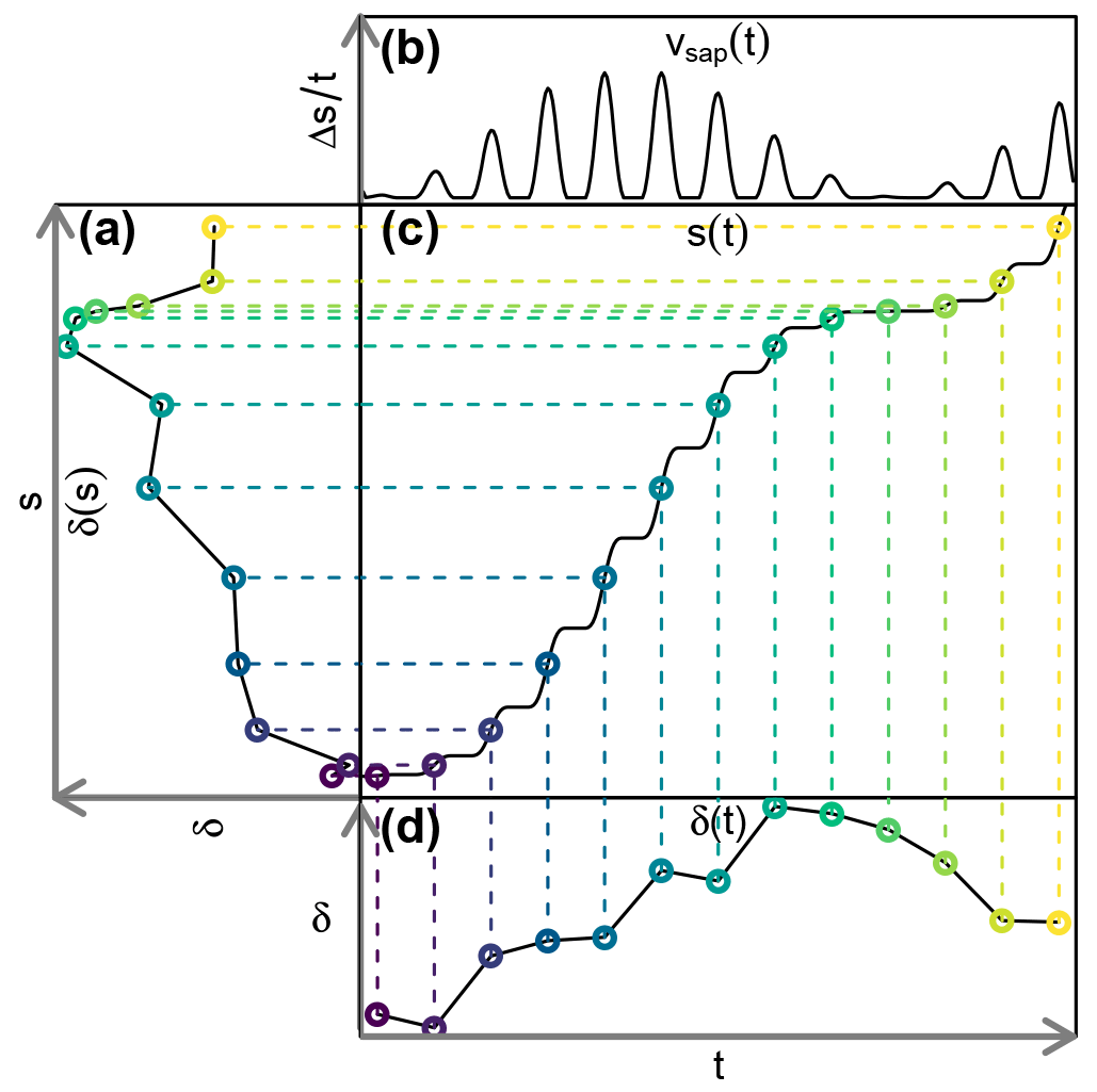
Figure 1Exemplary transformation of (d) a tracer concentration time series δ(t) to (a) a concentration function depending on the cumulative sap flow distance δ(s). A time series of (b) sap flow velocities vsap(t) is needed for the construction of (c) the auxiliary function s(t).
In order to neutralize the effects of sap flow velocity variations, we transform our observed tracer time series δ(t) to “sap distance series” δ(s). This transformation is depicted in Fig. 1 and it requires us to obtain a cumulative sap flow distance s for each time step t with the following equation:
where Δsi is the distance traveled by the sap during ti, and is the mean sap flow velocity of ti, which has a duration of Δti. With an established transformation between time t and sap flow distance s, we can transform observed tracer time series δ(t) to tracer “sap flow distance” series δ(s).
After the transformation of δ(t) to δ(s), we can predict the isotopic signature at the stem base, δxyl.R, by convolving δRWU with the FPLD between the stem base and all root tips (e.g., hR from Sect. 2.1.2):
Similarly, we can relate δxyl.R to δxyl.H (an isotopic stem xylem signature at a certain height above the stem base) by convolution with an appropriate transfer function that manages to represent the respective FPLD.
Eventually the methodology described in the previous sections can be combined as follows:
-
transform input tracer time series to input tracer sap distance series,
-
convolve input tracer sap distance series with an appropriate transfer function (representing a static FPLD),
-
transform output tracer sap distance series back into an output tracer time series.
2.2 Field experiment
2.2.1 Study site and instrumentation
The experiment described in this study took place at a research site located on a 25∘ steep hillslope of the Swabian Jura in southwestern Germany (47.98∘ N, 8.75∘ E, close to the city of Tuttlingen). The soil type is a Rendzic Leptosol developed on glacial slope debris of Jurassic limestone. Soil texture in the upper 70 cm ranges from silty clay to silty loam with a fraction of up to 43 % of rocks. Larger rock fragments can be found as shallow as 20 cm below the soil surface and become very abundant below 50 cm. Our 200 m2 experimental plot was situated within a stand of 90–100-year-old European beech (Fagus sylvatica) with diameters at breast height ranging from 45 to 90 cm and contained a total of four beech trees, of which three have been instrumented.
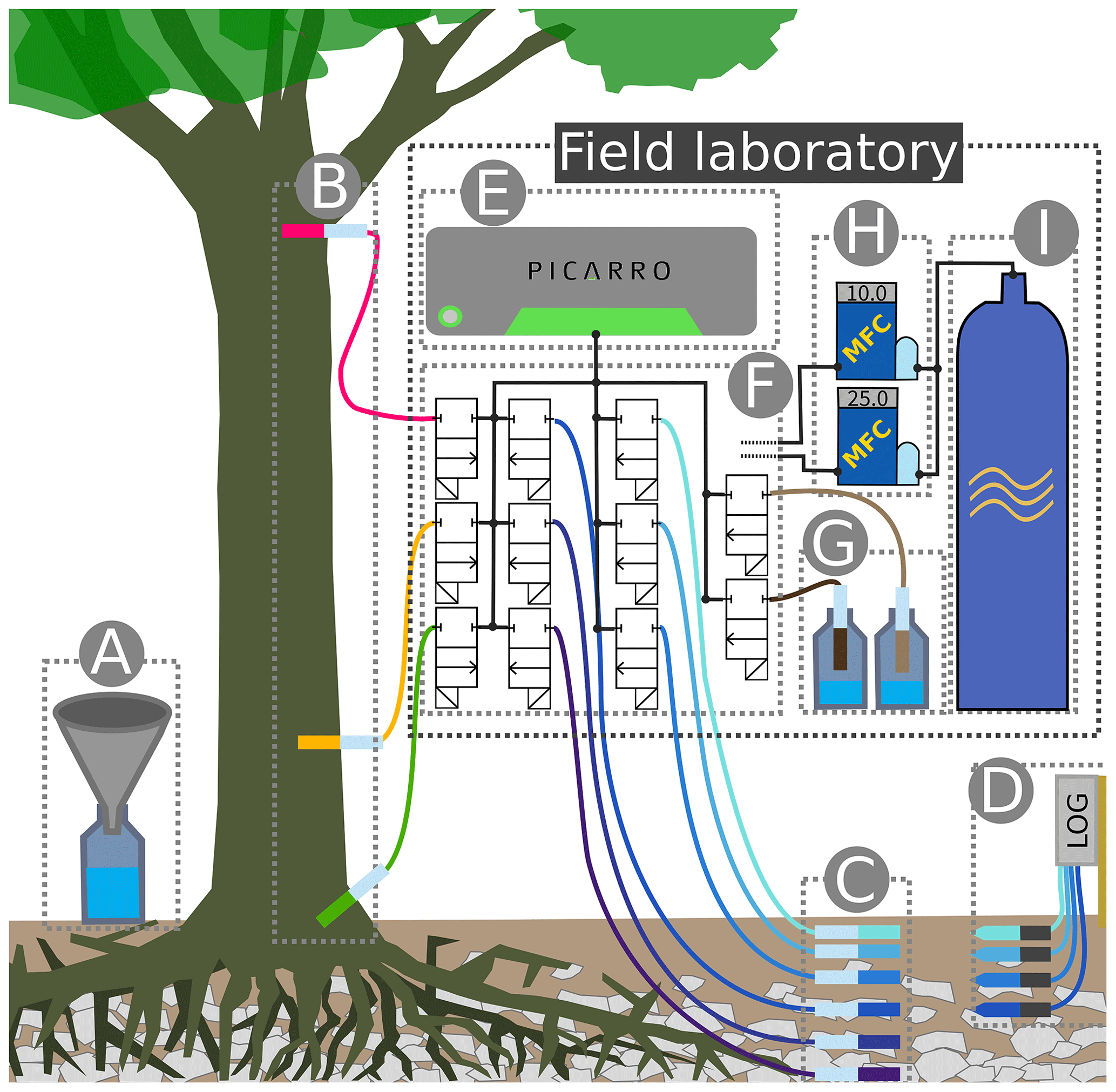
Figure 2Sketch of the experimental setup: (A) throughfall sampler; (B) WIPs at 10, 150 and 800 cm stem height; (C) WIPs in 10, 20, 40, 60, 80 and 100 cm soil depth; (D) volumetric soil moisture sensors in 10, 20, 40 and 60 cm depth; (E) CRDS for stable water isotope measurements; (F) valve system to sequentially connect each probe to the CRDS and the two mass flow controllers; (G) standard probes in headspace of liquid water standards; (H) mass flow controllers; (I) dry air for sample dilution and through-flow.
A sketch of the experimental setup is shown in Fig. 2, which omits the repeated instances of the principal components and sensors. Precipitation (throughfall) samples were taken as often as possible from four rain gauges (Fig. 2A) distributed on and around the study plot. One of those gauges was combined with a tipping bucket (0.2 mm resolution, Davis Instruments, Hayward, USA) in order to register hourly precipitation amounts. A total of four depth profiles of volumetric soil moisture sensors (SMT100, Truebner GmbH, Neustadt, Germany) were installed in depths of 10, 20, 40 and 60 cm (Fig. 2G) with different radial distances to the trees.
At depths of 10, 20, 40, 60, 80 and 100 cm we installed one profile of WIP into the soil (Fig. 2F). Additionally we installed WIPs into the xylem of two beech trees (T1 and T2) at 10, 150 and 800 cm height (Fig. 2B), as well as into the xylem of another beech tree (T3) at 150 cm height. The different installation heights are reflected by the probe IDs (e.g., T1R, T1B and T1H), where R stands for “root” (10 cm), B for “breast height” (150 cm) and H for “high” (800 cm). Depending on the locations of the probes and the trees, the tubing lengths between the probes and the CRDS varied between 5 m (T2R and T2B) and 20 m (T1H). Additionally, we put two probes into the head space of two sealed 1 L containers made of high-density polyethylene (HDPE), filled with 250 mL of water with known isotopic composition (Fig. 2E). These two probes acted as our light ( ‰, ) and heavy ( ‰, δD=6.63 ‰) reference standards and were placed directly next to the CRDS in our field lab.
In order to install the WIPs with a diameter of 10 mm into the tree xylem, we drilled a hole with a 10 mm wood drill, a strip of tape marking a hole depth of slightly more than the length of the 5 cm porous head. Care was taken not to overheat the drill in order to avoid singed xylem wood in the hole. Afterwards, a 10.2 mm metal drill was used to slightly widen the hole and clear out wood chip residue. Then the probe was firmly pushed into the hole just deep enough to place the porous head behind the phloem. In a final step, silicone was applied around the probe to seal the hole. While the silicone is curing, organic fumes may interfere with the measurements of the CRDS. Therefore it is advisable to install the probes several days before the scheduled start of the measurements. In addition, we placed heat-pulse-based sap flow sensors (East 30 Sensors, Pullman, USA) in the vicinity of each WIP. Measurements of the tipping bucket, soil moisture sensors and sap flow sensors were logged in 10 min intervals with a CR1000 data logger (Campbell Scientific, USA).
2.2.2 Tracer experiment
The stable water isotope concentrations for 18O and deuterium in this paper are noted in the δ-notation relative to Vienna standard mean ocean water (VSMOW):
where Rsample and RVSMOW are the DH or 18OO ratios of the sample and VSMOW, respectively.
Since no direct water source was available to irrigate the plot with a defined amount of 150 mm, 60 m3 of groundwater was trucked to the site and run through an industrial deionizer (VE-300 (6×50 L), AFT GmbH & Co.KG) to reduce the mineral content to low levels typically found in natural rainfall. In our case the sprinkling water had an electrical conductivity of around 20 µS cm−1 and an isotopic composition of ‰ and ‰. By mixing 1 kg of D2O with the 60 000 L of water within a collapsible pillow tank (custom made by FaltSilo GmbH, Bad Bramstedt, Germany), which was placed 100 m upslope of the experimental plot, we obtained deuterium-enriched irrigation water ( ‰, δD=40 ‰). On 21 May 2019, we used an array of six sprinklers (Xcel-Wobbler by Senninger, Clermont, USA) driven by the height difference between pillow tank and irrigation site, to distribute our prepared D2O–groundwater mixture onto the experimental plot. The amount of irrigation water actually reaching the core plot area of 10 by 20 m was equivalent to 150 mm rainfall within 8 h. After this artificial event, we continued to monitor the plot under natural conditions for another 12 weeks.
2.2.3 Stable water isotope measurement system
On 2 d prior to the irrigation, as well as 1 d after the irrigation, we took a total of five destructive soil core samples. We used an electric breaker (HM1812, Makita Werkzeug GmbH, Germany) to drive a core probe (60×1000 mm, Geotechnik Dunkel GmbH & Co. KG, Hergolding, Germany) into the soil until we hit larger rocks. The soil cores were extracted and split into 10 cm segments, yielding 120 to 300 g of fine soil and skeleton material per depth increment, which were filled into aluminum-coated coffee bags (WEBAbag CB400-420siZ, Weber Packaging GmbH, Güglingen, Germany).
Following the equilibration bag method after Wassenaar et al. (2008) and Garvelmann et al. (2012), the sample bags were filled with dehumidified air in the lab and permanently sealed with sealing tongs (Weber Packaging GmbH). After 24 h of equilibrium at constant temperature, the sample bags were punctured by a hollow needle connected to the inlet port of a cavity ring-down spectrometer (CRDS) stable water isotope analyzer (L2120-I, Picarro, Santa Clara, USA). After 5 to 10 min, the isotope analyzer readings reached plateaus of constant values. Before and after the measurements of the soil bags, we also measured three standard bags filled with liquid water of known isotopic composition, which were treated identically to the bags containing soil samples.

Figure 3Sketch of a WIP installed in soil. Water vapor from the surrounding medium (in this case soil) diffuses through the microporous membrane into the probe head (C). Before being sucked into the sample line (D), the sample gas is diluted within the mixing chamber (B).
The WIPs used in this study were built at the Chair of Hydrology of the University of Freiburg, Germany, following the “diffusion-dilution sampling” (DDS) design described by Volkmann and Weiler (2014). Figure 3 shows a sketch of a WIP installed in the soil. Key elements of a WIP are the mixing chamber (B) made of PVDF and a screw-on membrane head (C). This membrane head (manufactured by Porex Technologies, Aachen, Germany) mainly consists of a 50 mm long hydrophobic but vapor-permeable microporous cylinder made of PE with a pore size of 10 µm. From within the mixing chamber, the sample line (D) connects to the CRDS water isotope analyzer, which has a constant intake rate of about 35 mL min−1. Air and vapor from within the probe head reach the mixing chamber through a small connection hole and are sucked into the sampling line. The dilution line (E) is used to deliver dry air directly into the mixing chamber, which allows for a controlled dilution of the sampled air–vapor mixture, while the water outside of the probe and the air inside the probe head can still exchange under equilibrium conditions. The through-flow line (F) can deliver additional dry air into the system and helps to prevent underpressure as a result of dilution rates that are smaller than the constant sampling rate. Tests have shown that the gas exchange through the membrane head is so fast that it is not possible to dilute the sampled air through the through-flow line. All three lines of tubing utilized to deliver dry air into the probe or sample vapor from the probe are made of fluorinated ethylene propylene (FEP) and have an external diameter of 1.59 mm () and an internal diameter of 0.75 mm.
Deviating from the original applications of WIPs (Volkmann and Weiler, 2014; Volkmann et al., 2016a, b), we switched from using N2 as dilution and through-flow gas to compressed dry air. As Gralher et al. (2018) have shown, intrusion of ambient air has a considerably larger influence on measurements relying on N2, compared to measurements that use dry air as dilution and flush medium. Furthermore, transporting compressed dry air in a vehicle has fewer restrictions than transporting compressed N2. A pressure regulator reduced the pressure at the outlet of the compressed dry air bottle down to 1.5 bar. The dry air stream was split between two mass flow controllers (GFC17, 0–50 mL min−1 and MFC 35828, 0–200 mL min−1, both manufactured by Analyt-MTC GmbH, Müllheim, Germany).
Over custom manufactured valve manifolds (Horst Fischer GmbH, Gundelfingen, Germany), equipped with two-way electric valves (EC-2M-12, Clippard, Cincinnati, USA), each of the probes was connected to the two mass flow controllers and the sample inlet of the field-deployed CRDS stable water isotope analyzer (L1102-i, Picarro, Santa Clara, USA). Connections between the probes, valve manifolds, mass flow controllers and isotope analyzer were made with in. FEP tubing (Techlab GmbH, Braunschweig, Germany) and flangeless fittings (XP-220, IDEX, Lake Forest, USA). Connections between the dry air supply and the mass flow controllers were made with stainless-steel fittings (Swagelok, Solon, USA). We set up our field-deployed CRDS and its peripherals within a watertight container and supplied it with electricity from a nearby power line.
Based on the Arduino microcontroller platform (Badamasi, 2014), we designed and built a custom circuit board that is able to switch electromagnetic valves and to provide two independent analogue voltages. Those voltage signals were used to control the through-flow of two mass flow controllers. A custom-made Python-based software GUI that is able to interface the Arduino-based circuit board and interpret the CRDS' log files in near-real time enabled us to automate the measurement process to a large extent and to quickly adapt flow rates and times for flushing and measuring as well as the order of the probe sequence. We attached a USB modem (E531, Huawei Technologies, Shenzhen, China) to the isotope analyzer to regularly transmit summarized measurement results (less than 20 kB h−1) to an FTP server. With this setup, we could remotely monitor but not interfere with the ongoing measurements. Further details on this automation system (circuit board designs, assembly instructions and source codes of the control software) can be found in the following online repository: https://github.com/stseeger/IsWISaS (last access: 8 July 2021).
Table 1Threshold values for standard deviation s and trend index IT used for automated detection of stable measurement values.
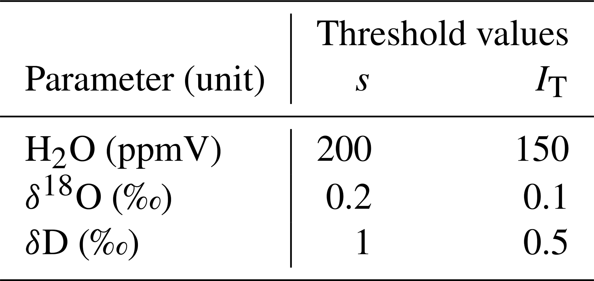
In order to obtain a measurement value for a certain probe, we activated the three respective valves of that probe (sample, dilution and through-flow line). The time of activation was saved to an automatically generated log file. At the same time, we initiated a flush phase by setting the dilution rate to the same as the CRDS' sample intake rate (in our case 35 mL min−1) and setting the flow rate in the through-flow line to zero. The duration of the flush phase was chosen depending on the overall tubing length of the probe – from 3 min for probes with short tubing up to 10 min for probes with 20 m long tubing. After the flush phase, we started the measurement phase by reducing the dilution flow rate to 10 mL min−1 and increasing the through-flow rate to 25 mL min−1 – dilution and through-flow yet again adding up to the constant sample flow rate of the CRDS. The measurement phase either ended after a fixed amount of time (in our case 20 min) or earlier, in case the measured raw values of the CRDS approached a stable plateau. Plateau detection was automated by checking standard deviations s and a trend index IT of the last 2 min of CRDS raw data for H2O (sample moisture content), δ18O and δD against the thresholds listed in Table 1. The standard deviation s was computed as
where N is the number of raw instrument readings within the last 2 min, are all of the respective values and is the mean of all these values. With the value of rounded to a whole number, the trend index IT was computed as
After each probe measurement, the system automatically proceeded to flush and measure the next probe within the specified probe sequence, which was automatically restarted upon its completion.
2.3 Data processing
From the raw sensor data, we computed the sap flow velocity vsap in m s−1 according to Campbell et al. (1991):
where k is the thermal conductivity of sapwood set to 0.5 (Hassler et al., 2018), Cw is the specific heat capacity of water at 4.184×10⁶ m3 K−1, ru and rd (both = 6 mm) are the distances of the central heater needle to the up- and downstream thermistor needles, and ΔTu and ΔTd refer to the temperature changes induced by the heating pulse at the up- and downstream needles, respectively.
Our measured sap flow time series was limited from May 2019 to 8 August 2019. In order to extend it to the whole year, we assumed no sap flow during the time where our deciduous trees did not have any foliage (before May and after October). During those periods, we set vsap to 0 m s−1. For the remaining period between 8 August and 31 October, we fitted the two parameters a and b of the following equation:
where VPD is the vapor pressure deficit (derived from meteorological data of the nearby meteorological site Klippeneck of the German Weather service DWD). In order to account for decreasing vsap due to leaf senescence, we multiplied the estimates obtained by Eq. (17) with a linearly decreasing reduction factor between the middle of September and end of October. Urban et al. (2015) reported a comparable autumnal reduction of sap flow in relation to potential evaporation for central European beech trees.
As an additional means to investigate RWU independently of isotope measurements, we followed Guderle and Hildebrandt (2015) and used measurements of volumetric soil moisture (averaged across the four available depth profiles) – more specifically the daily decline of soil moisture during dry days – as an indicator of RWU. To compare the soil moisture measurements with the RWU model, we derived a water uptake ratio rRWU in two ways:
where the first ratio defines the measured daily decline of soil moisture in the upper soil layer Δθu (average of 10 and 20 cm depth) and Δθl the equivalent for the lower soil layer (average 40 and 60 cm depth). The second ratio defines the relative modeled uptake strengths of Eq. (2) (with as the average of for the depths of 10 and 20 cm and as the average of for the depths of 40 and 60 cm). The soil-moisture-based computation of rRWU is limited to days where the soil water content throughout the depth profile is below field capacity.
In order to analyze the WIP measurements, we used the recorded valve switching times to aggregate the raw CRDS log file data by computing average values for the last 2 min of each period. The parameters of interest were sample water vapor content, δ18O and δD. In the next step we corrected for the influence of temperature on the fractionation factors during vapor equilibration at the probe head. Instead of direct temperature measurements, we relied on the assumption that the temperature at the place of equilibration (i.e., around the probe head) is reflected by the water vapor content of the obtained sample gas – given that the sample rate and the dilution rate are held constant. By computing linear regressions between measured vapor isotope values (δm) for our two standards and the sample gas moisture contents (Cm), we derived the slopes needed to correct all vapor isotope measurements to one reference moisture content value (Cr=18 000 ppmV) according to the following equation:
where δv is the corrected isotope value and ΔCδ is the slope obtained by the linear regression between Cm and δm values of the standards.
To infer the isotopic signature of the liquid water that equilibriated with the sampled vapor, we used the relationship between the known liquid phase values of our two standards and the respective observed vapor values:
where δl.x is the normalized liquid phase isotopic value of measurement x, δv.x is the moisture-corrected vapor value of measurement x, δv.L is the moisture corrected vapor value of the light standard, δl.L, is the liquid phase isotopic value of the light standard and ΔLH is the slope obtained by
with δv.H as the moisture corrected vapor value of the heavy standard and finally δl.L and δl.H as the known liquid water isotope values of the light and heavy standards, respectively.
Under stable environmental conditions, δv.L and δv.H should not change at all, but in a field experiment more frequent measurements of these standards are highly recommended. We treated both standards as regular parts of our measurement sequence, yielding one measurement of each standard every 3 to 4 h. For the normalization procedure we interpolated between those actually measured standard values in order to estimate the standard values for each measurement.
2.3.1 Modeling RWU, FPLDs and xylem water age
To obtain the necessary input data for RWU modeling, we interpolated our observations of volumetric soil moisture and soil isotopic signatures over time and space to generate a continuous time series in time and space. Lacking any observations below 60 cm for volumetric soil moisture and 1 m for soil water isotopes, we assumed constant boundary conditions (θ=25 %, ‰ and ‰) at the lower profile border in 2 m depth.
Subsequently, we used the Jarvis RWU model (see Sect. 2.1.1) to compute RWU isotopic signatures. Then we applied the convolution approach described in Sect. 2.1.2 in order to transfer the RWU isotopic signatures to the respective stem base xylem isotopic signatures, which could be compared to our in situ xylem water measurements at the stem base. Model performance was evaluated by computing the root-mean-square error (RMSE) between model predictions and observations for deuterium and 18O at the stem base as well as for the water uptake index rU (see Sect. 2.3). With as the ith of a total of n observations and yi as the respective simulated value, the RMSE was computed according to
Next, we evaluated the model for 500 random parameter sets within the value ranges given in Table 2. The soil related model parameters were assumed to be identical over the whole profile depth. Based on the observed soil moisture time series, we set the volumetric soil moisture at saturation θs to a fixed value of 45 %. Since soil moisture levels near saturation only occurred for a short time during the irrigation, we set the model parameter to a value of 100 %.
Table 2The different parameters used for RWU modeling and the transfer functions used to transform δRWU into δR (hR, hF1) and δR into δH (hF2). Meanings of the parameters are listed in Table A1.
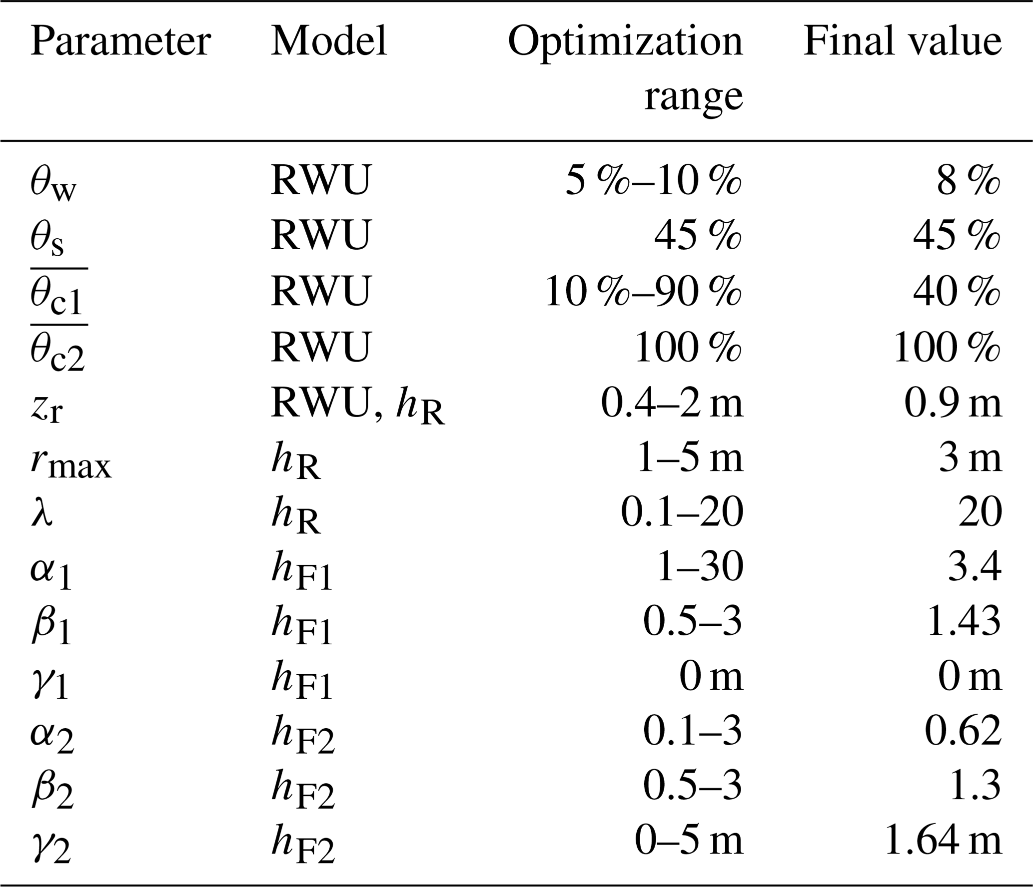
Eventually, to relate modeled RWU to our observed xylem isotopic signatures at stem heights of 0.1 and 8 m, we optimized FPLDs that can be described by the following parametric distribution:
with F being the probability density function of the Fisher–Snedecor distribution. The second parameter of F was set to a fixed value of 100, so that its first parameter α acts as shape parameter while the additional parameters β and γ act as scale and lag parameters, respectively.
Apart from simply predicting the transformation of δRWU during its transmission through a tree's xylem, the fitted FPLDs were also used to infer time variable xylem water age distributions. This was achieved by applying the approach described in Sect. 2.1.3 in combination with a series of virtual tracers, one for each time step with a concentration of 1 during the respective time step and 0 during all other time steps. The resulting tracer concentration time series were used to infer xylem water ages similar to Sprenger et al. (2016) (ages of percolation water below the root zone) and Brinkmann et al. (2018) (ages of RWU water). In contrast to the two mentioned studies, the water ages in this study refer to the time of tree water uptake, instead of the time of input as precipitation into the system.
3.1 Soil moisture and sap flow
The temporal dynamics of daily sap flow velocities and soil moisture (averaged across the two profiles on the irrigated plot) are depicted in Fig. 4a and b. Averaged for each month, the mean daily sap flow velocities varied between 42, 88, 94 and 85 cm d−1 for May (starting at 21 May), June, July and August (ending at 8 August), respectively.
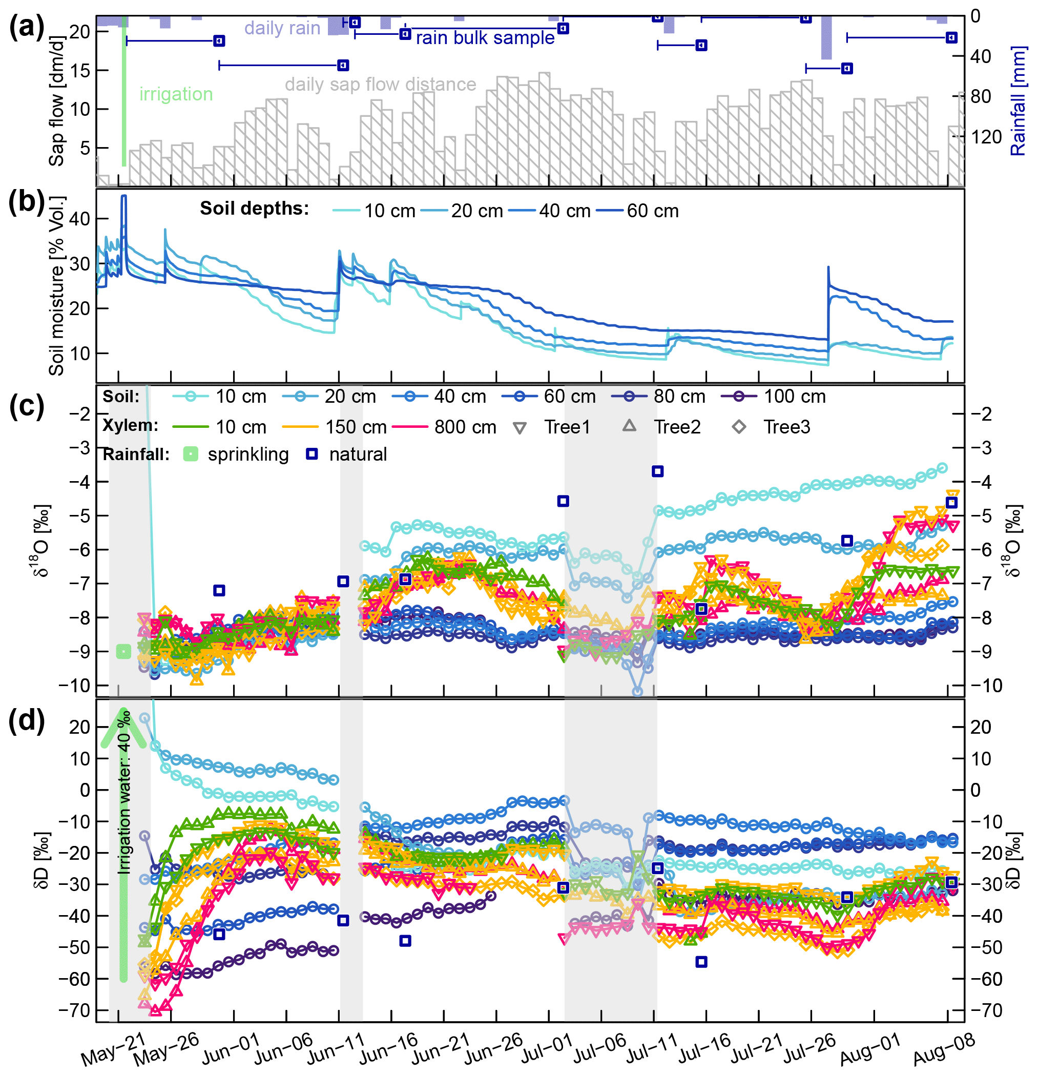
Figure 4(a) Daily rainfall and cumulative sap flow distances. Dark blue squares represent the mean rainfall amounts collected with the four bulk samplers (dark blue lines indicating the periods over which the bulk samples were collected). (b) Volumetric soil moisture at four soil depths. (c and d) Corrected time series of δsoil and δxyl in liquid water. The blue squares represent the mean isotopic signatures of the four bulk samplers. The translucent grey areas in (c and d) mark time periods with missing or unreliable isotope data.
The sprinkling experiment started on 22 May during a wet period with soil moisture around field capacity (ca. 30 Vol. %). From 1 to 10 June, the first dry period occurred, with soil moisture in the topsoil decreasing towards 15 Vol. %. Several rain events between 10 and 15 June rewetted the soil, but afterwards the soil moisture in all depths declined considerably. One rainfall event with 29 mm on 12 July caused a brief rewetting of the topsoil, and a heavy convective event with 52 mm on 27 July bypassed the upper two soil moisture probes and caused a strong increase by around 10 Vol. % at 40 and 60 cm depth.
The fitted Eq. (17) established a solid relationship (R2 of 0.85) between vsap and VPD (see Fig. A4a). Since there are no systematic discrepancies between measured and VPD-derived vsap values (see Fig. A4a), we have high confidence in assuming that the observed periods of reduced vsap during June and July (see Fig. 4a) can be attributed to temporarily lowered VPD instead of soil water deficits.
3.2 Stable water isotopes
In each measurement sequence 15 probes (two standards, six SWIPs and seven XWIPs) were measured within 3 to 5 h, resulting in one measurement every 12 to 20 min. The raw aggregated measurements and the correction procedure are described in Appendices A1 and A2. Some short-term fluctuations in the high-frequency data caused by diel air temperature fluctuations could be observed that could not completely be removed by the postprocessing procedures. Due to the large number of data points in the full data set and our interest in the overall temporal dynamics, we limited our further analysis to daily median values of the full data set, setting aside the development of a more robust diel calibration procedure for future studies.
Three of the xylem probes (T1B, T2B and T3B) exhibited a negative δ18O bias, which was corrected as described in Appendix A2.2. A comparison of the probe heads right after removal from the stem (12 weeks after installation) revealed that the membrane heads of two δ18O-biased probes were covered by biofilms while an unbiased probe did not show such a biofilm (see Fig. A6).
Focusing on the first period, between 21 May (date of the irrigation) and 10 June, the soil δD signature was rather stable, while δxyl increased for 6 to 14 d to reach a plateau. The δD signatures at the stem base at 10 cm height (green triangles in Fig. 4c and d) showed the steepest rise and reached their plateaus after approximately 6 d while the probes installed at 8 m height (pink triangles in Fig. 4) showed a delay of around 14 d. The δD signatures at 1.5 m tree height (yellow symbols) responded in between the former two groups.
The immediate post-irrigation δ18O signatures of the soil profile showed no considerable depth differentiation and little dynamics (see Fig. 4c). Following some smaller precipitation events with elevated δ18O signatures (−7.2 ‰ in rain compared to −9 ‰ in the soil), the soil signatures slightly shifted upwards. A similar development can be observed for the xylem δ18O signatures following the soil signatures. The larger rainfall event in the night between 10 and 11 June, followed by another 13 mm event on 15 June, influenced the soil isotopic signatures in two ways: the upper 20 cm of the soil was enriched in δ18O (2 ‰ to 3 ‰ more enriched than the lower soil depths), and the δD-enriched label water introduced with the irrigation was percolated further downwards. Following those changes in the soil isotopic signatures, we see the xylem δ18O signatures increasing by about 1.5 ‰ within 5 to 10 d. Simultaneously the xylem δD signatures decrease to levels close to the topsoil δD signatures.
We observed two periods 23 June to 11 July and 16 to 26 July that are characterized by declining soil moisture and rather constant δsoil. Both of these periods show the same pattern of δxyl further deviating from the isotopic composition of the topsoil and converging towards the values of the deeper soil layers. On the other hand, we also observed two rainfall events (12 and 27 July) that lead to a replenishment of soil moisture without considerable changes in δsoil. In both cases, we could see an opposite response to the dry period. δxyl was more similar to the isotopic composition of the upper soil layers and diverged from that of the deeper soil layers. The 18 mm of rainfall on 12 July was exhausted within the following days, and soil moisture (and δ18O signatures) quickly returned to the low levels before the event. The rainfall event on 27 July raised the soil moisture levels to such an extent that the low pre-event soil moisture did not recur within the observed time period.
3.3 Optimization of the RWU model
The temporally and spatially continuous soil moisture and soil water isotope data needed for the optimization of the RWU model were obtained by interpolation of soil sensor data, soil core measurements and SWIP measurements (see Fig. A5).
Subsequently, the optimization was carried out as described in Sect. 2.3.1. Figure 5 shows the results for the combined parameter optimization of the RWU model and the transfer function hR, which is used to convolve the modeled δxyl.RWU in order to obtain values for validation of δxyl.R. Each row in Fig. 5 belongs to one model output variable (δ18O, δD and the RWU depth distribution index rU) and was evaluated individually. The best 10 model simulations are depicted in blue, and 20 random samples drawn from the worst 50 %–90 % of all simulations are depicted in red/orange. The evaluation was done for the starting phase (dark blue and red) and for the full observation period (light blue and orange).
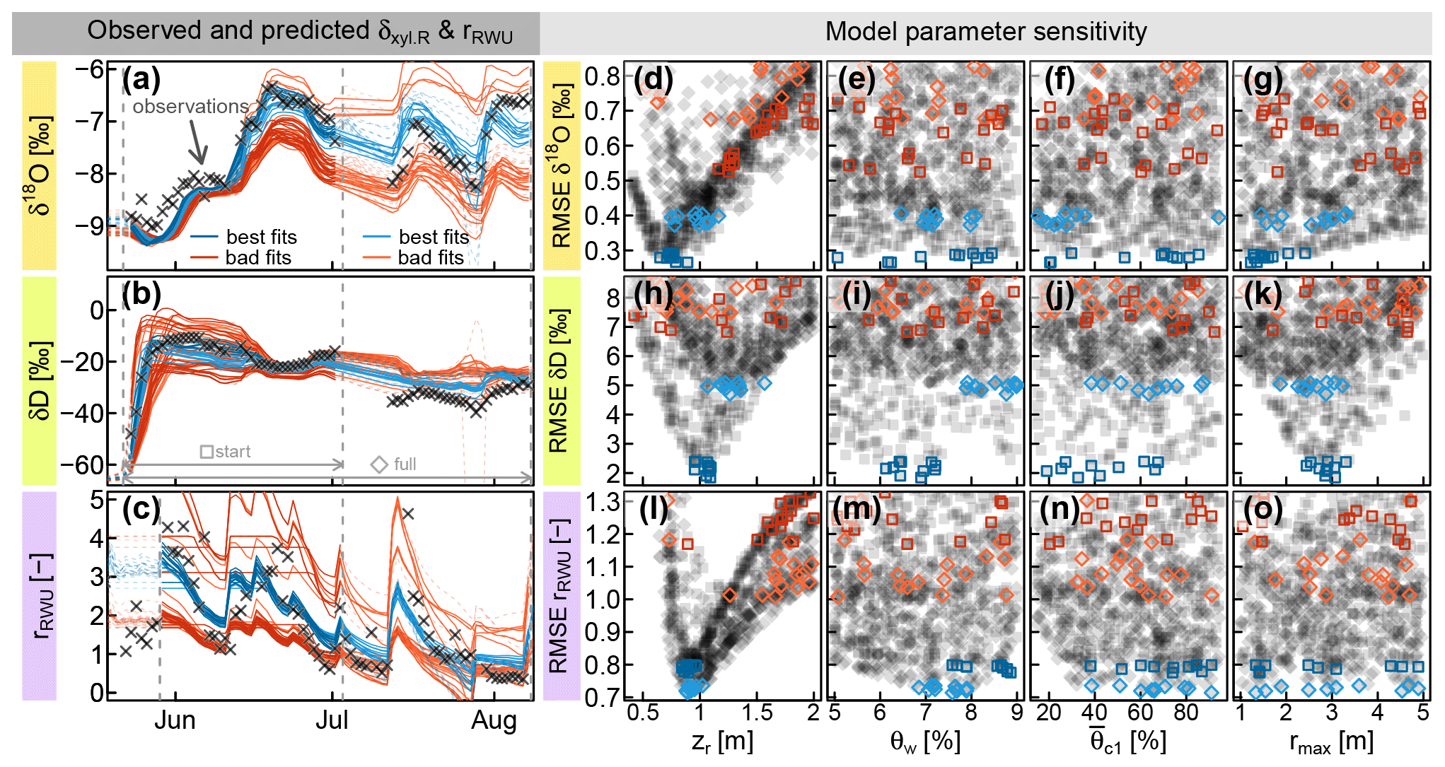
Figure 5(a and b) Observed δxyl.R (δxyl at the stem base, grey crosses) compared to model predictions of δxyl.R (lines), evaluated over the whole observational record (light blue and orange) or just the start phase (dark blue and red). (c) Root water uptake ratio rRWU derived from soil moisture measurements (grey crosses) and RWU simulations (colored lines). (d–o) RMSE values between observed signatures and simulated signatures in relation to the model parameters zr (rooting depth), θw (wilting point soil moisture) (critical normalized soil moisture of water stress onset) and rmax (maximum lateral root extent). The parameter combinations leading to the selected colored time series in (a–c) are colored identically in the respective (d–o).
When only the first half of the observational record is considered (darker blue squares and lines), both isotopes show a parameter optimum for zr (rooting depth parameter) between 0.75 and 1 m (see Fig. 5d and h). For that period, it was not possible to identify the optimal parameter value for the other two (water-stress-related) RWU parameters θw and , which seemed to be rather insensitive to both isotopes (see dark blue squares in Fig. 5e, f, i and j).
The maximum lateral root extent rmax was critical to reproduce the rise of the deuterium signal after the irrigation and showed a clear optimum around 3 m (Fig. 5k). The lateral root density decay parameter λ (not depicted in Fig. 5) proved to be far less sensitive than rmax, but there was a clear tendency towards values of λ below 1, implying a faster-than-linear decrease in horizontal root densities. When the full time period was considered (light blue diamonds and lines), the optimal values for zr were found at deeper depths between 0.9 and 1.5 m (see Fig. 5d and h). The optimal wilting point soil moisture θw ranges between 6 %–8 % and 7 %–9 % (for δ18O and δD, respectively; see Fig. 5e and i).
Unlike the two water isotopes, the water uptake ratio rRWU relies on soil moisture data alone and is not involved in the convolution step. Consequently, rmax was completely insensitive to rRWU. With respect to rRWU, optimal zr values were found between 80 and 100 cm, which is in good agreement with the isotope-based zr values in the start phase of the observational record. Based on rRWU, the optimal θw values are between 7 % and 9 % (see Fig. 5m), and the optimal values are between 30 % and 100 % (see Fig. 5n).
3.4 Optimization of xylem FPLDs
Based on the optimized RWU model, we could compare modeled δRWU to measured δxyl values. Except for the deuterium signatures towards the end of the experiment, there was a good agreement for both isotopes (see Fig. 6). However, in cases of abrupt δRWU changes, the observed δxyl values did respond with a delay which increased with stem height. This was most obvious after the deuterium labeling (box A in Fig. 6b). In order to account for the expectable delay that occurs during the transport of water from the roots along the xylem, we optimized FPLDs to transform our modeled δRWU values into δxyl values.
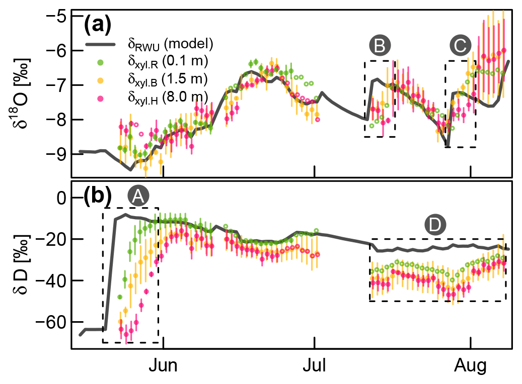
Figure 6Measured δxyl (colored dots) compared to the modeled δRWU (grey line). δxyl values were averaged across all available probes at each of the three installation heights. Vertical bars indicate the value range of all available (two to three) probes, and empty circles without lines indicate single probe values. Dashed boxes (A), (B) and (C): periods, where observed δxyl apparently lags behind changes in modeled δRWU. Dashed box (D): clear bias between modeled δRWU and measured δxyl.
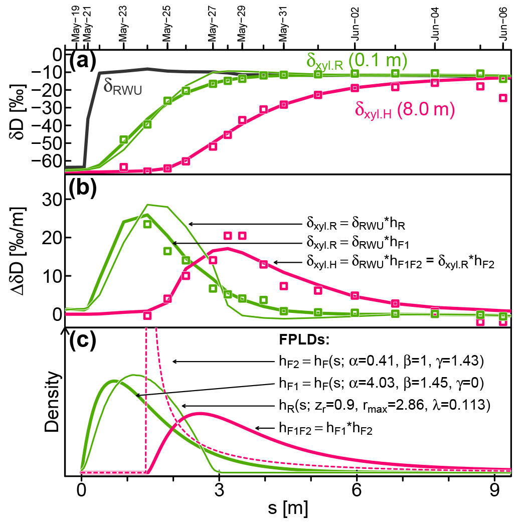
Figure 7Measured (squares) and modeled (lines) isotopic signatures of RWU(δRWU) and xylem water at the stem base (δxyl.R) and at 8 m above the ground (δxyl.H). (c) The FPLDs used to transform the modeled δRWU to δxyl as depicted in (a) and (b). The “*” operator stands for convolution.
Figure 7 shows observed (squares) and modeled (lines) δRWU (grey) and δxyl (green and pink) values. The original time series was transformed into the sap distance domain (see Sect. 2.1.3) in order to eliminate the influence of time-variable vsap, which was lower at the start of the depicted period and higher towards its end. Figure 7b depicts the same data as Fig. 7a but plots their rate of change instead of their absolute values. The colored lines in Fig. 7a and b are the results of convolutions of the modeled δRWU signature with different FPLDs (depicted in Fig. 7c).
In order to transform δRWU into δxyl.R, we convolved it with two different transfer functions: (1) the conceptually grounded hR (thin green line, defined in Sect. 2.1.2), whose parameters were optimized together with the RWU model parameters, and (2) the empirically, more flexible hF1 (thick green line, defined in Eq. 23), whose parameters were optimized subsequently to reach the best possible fit to observed δxyl.R values. The overall shapes of hR and hF1 turned out to be similar, but the latter achieved a much better fit to the available δxyl.R observations, while the former failed to adequately reproduce the right-skewed, tailed shape required to fit the observational data (see Fig. 7b).
Following this, we simulated the signal transformation of δxyl.R (at the stem base, thick green line) into δxyl.H (at 8 m stem height, thick pink line) by convolving δxyl.R with another transfer function, hF2 (dashed pink line in Fig. 7c), whose parameters were optimized to reach the best possible fit to observed δxyl.H values. In contrast to hF1, hF2 features a notable time lag around 1.4 m at the beginning and has a strong peak. Its tailing is similar to that of hF1.
To directly transform δRWU into δxyl.H, it can be convolved with hF1F2, which is the convolution of the two FPLDs hF1 (root tips to stem base) and hF2 (stem base to 8 m stem height).
According to the shape of hF2, the largest fraction of a signal between the stem base and a stem height of 8 m arrives after 1.4–2 m of cumulative sap flow distance. This may seem like a paradox, but it is not. The sap flow distance s is derived from heat-probe-based vsap, which other studies (Meinzer et al., 2006; Schwendenmann et al., 2010) have reported to be considerably lower than vδ (transport velocity inferred from isotopic tracer observations). Based on our observations, we can infer vδ between the stem base and 8 m stem height to be about 5.5 times faster than vsap.
3.5 Xylem water age distributions
In order to compute temporally variable distributions of xylem water ages at a certain stem height, two things were required: (1) a transfer function representing the FPLD between root tips and the stem height of interest, i.e., hF1 and hF1F2 as determined within the previous section and (2) a sap flow time series.

Figure 8Selected quantiles of modeled xylem water ages at 0.1 m stem height (green) and 8 m stem height (pink) based on FPLDs hF1 and hF1F2, respectively, and time-variable sap flow velocities. Panel (b) shows the subset of (a) which is marked by the blue rectangle.
We extended our measured sap flow time series beyond its original range over a full year as described in Sect. 2.3 (see Fig. A4b for the complete extended vsap time series). Subsequently, we duplicated this extended vsap time series in order to obtain enough data for an appropriate warm-up period for the following computations.
By combining sap flow velocities, FPLDs, and virtual tracers for each day (as described at the end of Sect. 2.3.1), we obtained xylem water age distributions at 0.1 and 8 m stem height. In Fig. 8 the time variable age distributions are represented through specific quantiles between 0 % and 99 % for 8 m stem height. For clarity's sake, only the median water age is depicted for 0.1 m stem height.
Figure 8a shows the xylem water ages over the course of a year between the ends of two vegetation periods. During the dormant season (November–May) xylem water is immobile, and consequently its age increases by one day per day, eventually exceeding ages of 200 d and more. At the start of the growing season, xylem water ages drop sharply, as soon as fresh uptake water has replaced the previous season's water, which happens earlier at the base of the tree stem.
Figure 8b focuses on the growing season of our field experiment. At the start and towards the end of the growing season, xylem water ages are considerably larger than during the main growing season. From the beginning of June to the middle of September the median xylem water age at 8 m stem height varies between 2.3 and 8 d with a mean value of 4.7 d. Median xylem water ages at 0.1 m stem height in the same period are lower and range between 0.4 and 3.8 d with a mean value of 1.6 d.
4.1 Performance of the measurement setup
By complementing the measurement system of Volkmann and Weiler (2014) with a sophisticated hard- and software framework to control the required gas flow controllers and solenoid valves, we developed a system capable of largely unattended long-term operation. As all of the additional components were built from readily available parts, our extension of the original setup did not notably increase the overall cost, which is mainly set by the CRDS itself and to a smaller degree by the required probes and valves.
Up to this date, our setup is the most complete field-tested in situ stable water isotope measurement system for continuous ecohydrological investigations. It contains many of the elements of the “ideal system” sketched by Beyer et al. (2020). To summarize, we list the main advantages of the use of WIPs compared to other in situ measurement techniques.
-
To install WIPs into the soil, it suffices to dig or drill a hole with a diameter of around 30 cm. Multiple WIPs (in different depths, at different sectors of the hole) can then be pushed into practically undisturbed soil. The installation of loops of gas-permeable tubing into the soil, as used by Rothfuss et al. (2013), Oerter and Bowen (2017), and Kübert et al. (2020), is much more invasive and will inevitably disturb the observed soil to a higher degree.
-
The borehole equilibration method by Marshall et al. (2020) relies on boreholes that go all the way through the tree stem. Consequently, with increasing stem diameters, the measurements of this method will increasingly be influenced by the isotopic signature of immobile water from the heartwood. Possibly up to a point where the dynamics of the mobile water transported in the outer parts of the xylem gets hard to detect. WIPs on the other hand are always probing the outer 5 cm of the stem xylem – similar to the depths measured with many sap flow sensors.
-
By directly diluting the sample gas within the WIP's mixing chamber, condensation within the sample line is avoided without the need for additional heating of the whole sample line. Additionally, there is an easy way to test the airtightness of the measurement system, by checking how dry a highly diluted sample gets – if it remains moist at maximum dilution rate, there must be some source of moisture (i.e., condensed droplets) between mixing chamber and analyzer or other leaks.
-
The identical design of WIPs in soil and xylem provides a consistent measurement method for soil and tree xylem. This can be considered an advantage compared to in situ methods that are only suited for soil (Rothfuss et al., 2013) or xylem (Marshall et al., 2020). The use of one single type of probe simplifies automating the measurement procedure and interpreting the obtained measurements.
We encountered some issues with partially biased δ18O XWIP measurements, similar to what Volkmann et al. (2016b) have reported. Since not all XWIPs exposed such a δ18O bias, we hypothesize that the occurrence of the encountered bias is related to the observed formation of biofilms on the XWIP probe heads (see Fig. A6). Those biofilms might have promoted the emission of volatile organic compounds which have been reported to interfere with CRDS stable water isotope measurements (West et al., 2010; Chang et al., 2016). However, even when the δ18O measurements seemed biased, they exposed similar temporal dynamics as unbiased measurements, and all of those dynamics agreed with what our proposed modeling framework predicted. So even though we may not be completely sure how to reliably rule out the formation of δ18O-bias-inducing biofilms, which are potentially favored by the design of our probes compared to the more aerated approach of Marshall et al. (2020), we are confident that the observed temporal dynamics will still contain valuable information. If unbiased xylem measurements or observations of soil isotopic data are available, a bias correction should always be possible.
Considering the expected spatial heterogeneity of a skeleton-rich, clayey soil – on top of the spatial heterogeneity of infiltration patterns within forest stands (Goldsmith et al., 2019) – and the relatively slow temporal dynamics of the observed soil isotopic signatures, future investigations might benefit from an increased number of WIP soil profiles at the cost of a lower temporal resolution of soil isotope measurements.
4.2 Standards and calibration
Our standard probes were sampling the vapor from the headspace of sealed containers filled with waters of known isotopic composition. This contrasts to other practices of using soil standards (Beyer et al., 2020), prepared from dried soil material that was rewetted with standard water. The main reason of using headspace standards was the situation that the maximum number of WIPs in our setup was limited and that such soil standards may not be representative for xylem isotope measurements. Furthermore, the sampling of field soil for a “representative” soil standard is problematic when soil properties vary with depth – a standard suited for one horizon may lead to biased results for another horizon. Furthermore, Gaj et al. (2017) have shown that clay minerals may lead to isotopic fractionation when labeled water is applied to oven-dried clay-rich soils. This might lead to biases that are difficult to attribute to the different samples, and hence liquid water standards may be the better choice.
For a WIP with fixed dilution rate placed in the headspace of a liquid water standard with variable temperatures, we found a close relationship between the sample gas' vapor concentration and isotopic composition (see Fig. A2). As long as the air entering our probes is vapor saturated (which has been shown to be the case for soils by Volkmann and Weiler, 2014, while Marshall et al., 2020 have computed very fast saturation within the tree xylem), the sample gas vapor content is directly related to the temperature of the sampling location. Therefore, we ended up with a calibration procedure that uses the sample gas vapor concentration, which is automatically measured by the CRDS, instead of measured temperatures at the sampling locations. When all measurements of one probe per day were averaged, the resulting time series were reasonably consistent on a day-to-day scale. On a shorter timescale we observed fluctuations (for xylem and soil probes, but with clearly more pronounced fluctuations for soil probes closer to the surface), which were likely artifacts of insufficiently compensated temperature effects. A calibration procedure that explicitly considers observed temperatures at each WIP might help to dissolve these sub-daily fluctuations and therefore improve the measurement accuracy and enable the exploitation of the full temporal potential of these high-frequency in situ measurements. But the proper consideration of temperature effects is difficult under field conditions, especially when considering tree stems, where strong temperature gradients can occur at small spatial extents (see Derby and Gates, 1966). Even for laboratory conditions, Rothfuss et al. (2013) reported a mismatch between their measurements and the Majoube (1971) equation to compute the isotopic fractionation between the liquid and the vapor phase under equilibrium conditions as a function of temperature.
4.3 Process-based RWU modeling
We were able to identify meaningful parameters (zr, θw and rmax) for our process-based RWU model. This model in turn was suited to predict δRWU. Our approach of driving the RWU model directly with (interpolated) measured data avoided the difficulties that are likely to occur during the simulation of water transport within highly structured, skeleton-rich soil. Yet, our data-driven approach prevented problematic parametrizations of the RWU model from accumulating errors over consecutive time steps as would happen when the model itself had to keep track of soil moisture and soil water isotopic composition. Consequently, the critical model parameters θw (wilting point) and (onset of uptake reduction) were not identifiable (θw was insensitive when optimized against isotope data but was identifiable when optimized against soil moisture).
Regarding the RWU δD signatures, there is a notable mismatch for the second half of our observation period: the model systematically predicts more enriched δRWU values than we could measure at δxyl. Since all of the measured soil δD values during that period were more enriched than the observed δxyl, this is not a failure of the model itself, but rather a consequence of insufficient model input data. This could hint at deeper uptake depths which were not covered by the SWIP depth profile, the general lack of representativeness of one single SWIP profile due to soil heterogeneity or in the worst case a systematic bias in XWIP δD measurements as an aftereffect of the 10 d measurement interruption in July.
4.4 Interpretation of FPLDs
Unlike most hydrological catchments, where FPLDs change with the length of the flowing stream network (van Meerveld et al., 2019), the tree xylem may be considered to feature a static FPLD which is constant irrespective of the occurring transport velocities. Consequently, xylem water ages are determined by a static FPLD and time variable tracer transport velocities (vδ). While it is nearly impossible to monitor vδ with a high temporal resolution, vsap can be used as a proxy for vδ.
Previous experiments have shown that vδ may exceed vsap by several hundred percent. Meinzer et al. (2006) reported vδ to be 5 times higher than vsap, and Schwendenmann et al. (2010) even reported it to be about 16 times higher than vsap. In controlled laboratory experiments, Steppe et al. (2010) observed gravimetrically determined flux rates to be 3.7 times higher than heat-pulse-derived vsap without wounding correction (which we also did not apply). In order to derive vsap from heat pulse probe measurements, a value for the thermal conductivity of sapwood (see Eq. 16) is needed. We took this value from another publication (Hassler et al., 2018), but we cannot be sure whether the used value is actually appropriate as the authors of the cited study did not specify how they came to this value. Additional assumptions would be necessary for the wounding correction, but as Steppe et al. (2010) reported, the heat pulse method can be expected to underestimate actual flux rates even after the wounding correction.
Regarding all these complications to relate heat pulse base estimates of vsap to actual flux velocities, we can say that it is no surprise that we observed a mismatch between vsap and vδ. On top of that, heat-pulse-based estimates of vsap are based on point observations from a limited number of depths (in our case 5, 17.5 and 30 mm), whereas the actual sap flux has a continuous depth profile of varying velocities (Gebauer et al., 2008). Our WIPs sample the xylem from 0 to 50 mm depth, which in case of a distinct velocity gradient within that range might lead to a disproportional weighting of the actual sap flux passing the probe.
Nevertheless, the studies of Meinzer et al. (2006) and Steppe et al. (2010) indicate that vsap measurements should be a good proxy for fluctuations of vδ, even though the actual values can be expected to be scaled differently. The discrepancy between the fitted γ value of 1.43 m of hF2 in the sap flow domain (see Fig. 7c) and the corresponding real-world distance of 7.9 m between stem base and 8 m stem height is a consequence of the systematic underestimation of vsap due to the discussed issues with heat pulse probe methodology. Consequently, all of the fitted FPLDs should be rescaled by a factor of 5.5. However, as long as the only goal is to account for relative differences of flow velocities (opposed to the attribution of certain physically observable properties to the shape of the fitted FPLDs), the scaling factor between actual and apparent vsap is irrelevant.
Our conceptually derived hR, which was based on assumed vertical and lateral root distributions, proved suited to act as FPLD between δRWU and δxyl.R Yet, due to a lack of observations of lateral root distributions, we had to estimate an appropriate value for the maximum lateral root extent rmax via model parameter optimization, where rmax was identifiable when the model was evaluated with respect to δxyl.R. Given the uncertainties arising from measurement precision and accuracy, as well as spatial heterogeneity of the soil, it turned out that the robustness of an rmax estimate greatly improves with a distinct artificial isotopic labeling pulse.
However, the overall shape of the conceptually derived hR was unable to fully reproduce the skewness and tailing of the fitted parametric distribution hF1 (from Eq. 23), which produced an even better fit to the observed data. The observed tailing might be a consequence of an unexpected lateral root distribution, but it is more likely to be caused by dispersion during the root xylem passage, which is not directly accounted for within the applied convolution modeling approach. Other than the conceptually based hR, the distributions that can be achieved with different parametrizations of Eq. (23) (i.e., hF1 and hF2) seem to be able to implicitly account for the supposedly observed dispersive component of the tracer transport – at the cost of the interpretability of the optimized parameters. More elaborate modeling approaches that explicitly account for the effects of dispersion and diffusion should be able to yield both: physically meaningful model parameters and a good fit between simulated and observed tracer time series. Yet, such explicit modeling approaches would quite likely have a much higher computational cost than our simplified convolution approach and might require more extensive input data.
Future labeling experiments with sequentially applied tracer pulses limited to certain radial distances from the stems of trees with different characteristics, combined with more process-based modeling approaches, could help to study macroscopic and microscopic factors that shape the FPLD of a tree's root xylem.
4.5 Xylem water ages, FPLDs and their implications
During the main growing season 50 % of all xylem water passing the stem base of our studied beech trees was older than 1.6 d. When looking at the 8 m stem height, the mean median xylem water age was 4.7 d. Assuming the xylem water transport velocities are not changing fundamentally above that point, we can estimate that the mean median water age of the xylem water within the tree crowns of our studied trees was close to 10 d. Towards the fringes of the growing season, we can expect considerably higher water ages. This has to be kept in mind for any type of xylem water sampling in order to investigate RWU, specifically after rainfall events or artificial isotopic labeling, but also during periods where water stress may lead to changes in δRWU.
Previous studies (James et al., 2003; Meinzer et al., 2006; Schwendenmann et al., 2010; Gaines et al., 2016) have typically investigated aboveground xylem water transport via injection of isotopic tracers into the stem, and they gathered valuable data regarding the transport processes between the stem base and crown branches or leaves. However, by injecting their tracers above the ground, they did not capture the below-ground component of xylem water transport, between all individual root tips and the stem base.
Knighton et al. (2020), citing the study of Gaines et al. (2016), claimed they had “estimated time lags between RWU and transpiration”, while they had actually estimated time lags between tracer injection to the stem base and transpiration. Similarly, De Deurwaerder et al. (2020) propose a modeling framework that erroneously equates δRWU to δxyl at the stem base, leading them to the prediction of unlikely clear δxyl signals further up the stem. The FPLD between root tips and stem base (hF1 in Fig. 7c) contributes considerably to the smoothing of δRWU, much more than the FPLD along the first 8 m of stem height (hF2 in Fig. 7c). Consequently, we strongly suggest including the below-ground fraction of the tree in any endeavor that aims to simulate the propagation of δRWU along the stem.
At that point, it is important to note that most of the root system FPLD's distribution form results from its spatial configuration, featuring not only a depth density distribution, but also a lateral abundance (lateral density combined with projected area) distribution. Nevertheless, the often used simplified vertical 1-D representation of the soil–plant system for RWU investigation purposes does not necessarily have to be expanded by a second dimension: a computationally efficient way to account for vertical and lateral root distributions can be achieved by convolution of δRWU with an appropriately shaped FPLD.
This study demonstrated the application of a measurement setup which facilitates unprecedented high-frequency monitoring of stable water isotopes in soil and tree stem xylem. We were able to predict the observed time series of xylem water isotopic concentrations at different stem heights with a combination of a process-based RWU model and a convolution-based approach that accounts for the FPLD between root tips and the sampling points in the tree stem.
Our results showed that δRWU and δxyl are often similar but not necessarily the same. No δxyl measurement can represent actual δRWU: it will always be an integration over certain fractions of δRWU from different points in the past. Only under certain conditions (i.e., little temporal variability of the RWU composition or short transport distances combined with high xylem water transport velocities) can FPLDs within the plant safely be neglected. During our experiment we could identify three periods (one after the irrigation and two after natural rainfall events) with a notable discrepancy between δxyl measurements and modeled δRWU which could be attributed to the temporal dynamics caused by the plant xylem's FPLD. For those periods, the assumption that a tree's xylem water isotopic signature is equivalent to the isotopic signature of RWU has to be rejected. Consequently, tree water isotope models should account for the FPLDs between RWU and the sampling point used for model evaluation.
Furthermore, we conclude that a conceptual representation of a tree's root system is capable of reproducing the basic shape of the FPLD between δRWU and δxyl. But more detailed observations and experiments are needed before tree root xylem FPLDs can robustly be derived from observable tree characteristics and the tree architecture.
Due to the smoothing effect of FPLDs, sub-daily observations of tree xylem water isotopes are unlikely to reveal much information about short-term RWU dynamics. Except for precipitation events, soil water isotopes show even smaller temporal dynamics. Consequently, future investigations of stable water isotope dynamics should favor an increased number of probes in soil and xylem to cover spatial heterogeneity over high subdaily measurement frequencies.
A1 Raw in situ measurements
Table A1Abbreviations and parameter symbols used within this article and their meanings.
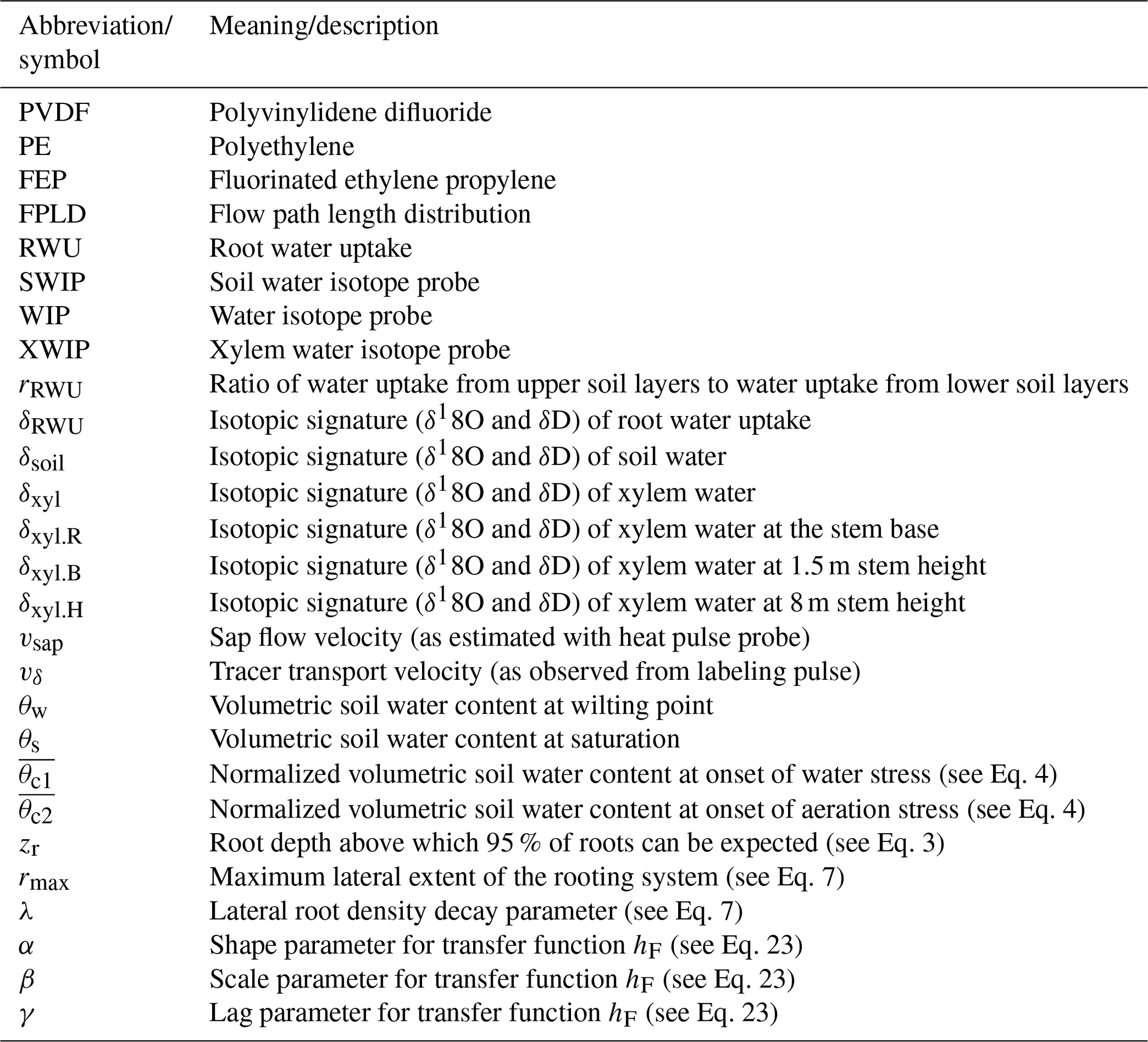
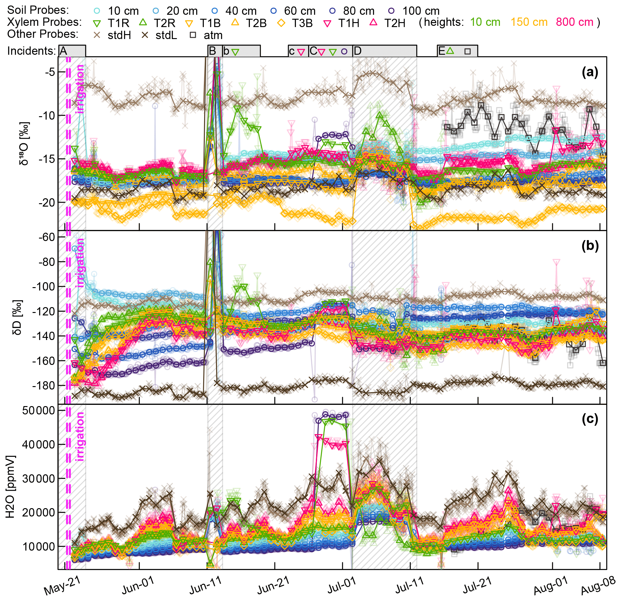
Figure A1Aggregated CRDS raw data (stable water isotopes and moisture) of all WIP measurements. Solid points indicate median values of daily measurements, while actual values are indicated translucently. Above the plots several incidents are indicated and numbered with letters. In case no symbols are associated with the incident, all probes are affected otherwise just the ones indicated. (A) Initial phase with some unreliable data. (B) Intrusion of water (through probe T1R) into the system during a high-intensity rainfall event. (b) Aftermath of (B); probe T1R still contains liquid water. (c) (C) Effects of strong winds and frail setup lead to loosened electric connections, deactivating the valves of three probes. (D) Interruption of dry air supply, no dilution and no through-flow. (E) Tubing of probe T2R was severed by rodents; from then on the system measured the atmospheric air on this valve slot.
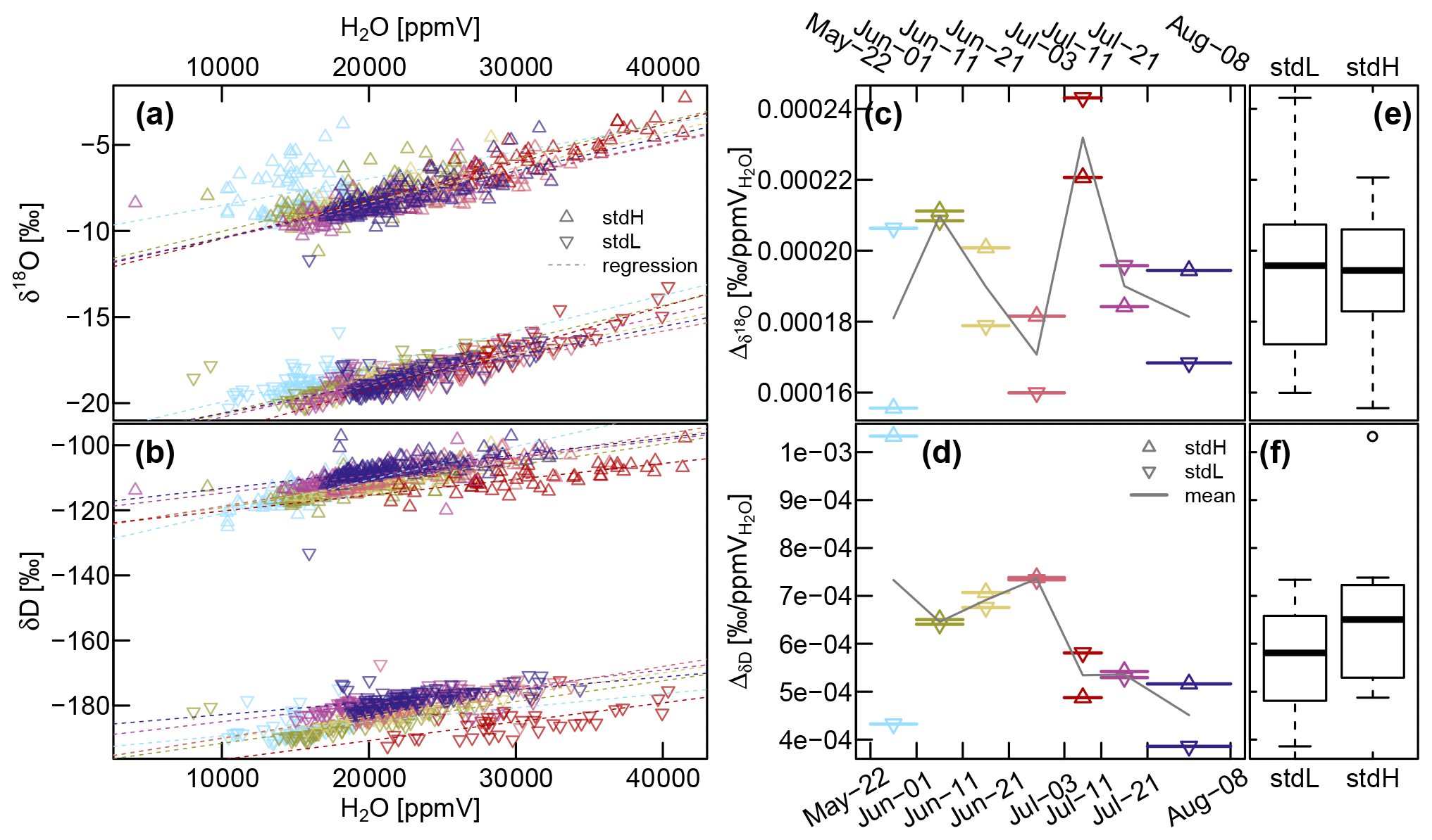
Figure A2(a and b) Relationship between sample gas volumetric moisture content (H2O [ppmV]) and the measured isotope values assessed with the heavy standard (stdH) and the light standard (stdL). The seven colors represent specific sub-periods, as used in (c) and (d), which show the variability of the slopes of the regression lines over time. The boxplots shown in subfigures (e) and (f) summarize this information. The blue period at the end of May indicates some starting problems, and the red period at the start of July demonstrates the effect of malfunctioning dilution.
Figure A1 shows the aggregated (averaged last 2 min before valve switch) CRDS raw data for both stable water isotopes (Fig. A1a and b) and the sample gas moisture content (Fig. A1c). The measurement sequence including 15 probes was completed every 3 to 5 h, resulting in one measurement every 12 to 20 min. The standards and the xylem probes showed a greater temporal variability resembling diurnal temperature fluctuations, while the thermally better insulated soil probes yielded more constant values over the day. Since the high-frequency data seem to be dominated by those temperature-related diurnal fluctuations and there are so many data points, we chose to focus on daily median values, which are plotted as solid in Fig. A1, while the underlying data points are plotted transparently in the background. On top of Fig. A1 we indicate some incidents that need to be commented on.
(A) We missed measuring the initial conditions, and our first measurement days might have been impaired by moisture within our measurement system that first had to be flushed out over time.
(B) During a rainfall event, stem flow intruded along the shaft of an insufficiently sealed WIP (T1R) diagonally installed into a tree root. After the water had entered the system around early 11 June, subsequent measurements of all other probes were unusable until we managed to visit the field site on 13 June to manually flush all tubing with dry pressurized air. Then we renewed the silicone sealing to protect probe TR1 from further water intrusions. While all other probes were back measuring, probe TR1 needed 5 more days to return to its normal operation.
(C) During a storm event, some cable connections became loose, starting with probe T1H, and a few days later continuing with the neighboring probes T1R and (SWIP) 100 cm. The valves for those three probes did not switch, and the CRDS's vacuum pump sucked its sample gas through the least airtight point in our assembly, rendering the respective data useless.
(D) Some time after changing the gas cylinder holding the dry air at 2 July, a seal failed – emptying the gas cylinder much faster than expected. Due to a holiday leave it was not fixed before 11 July.
(E) Some animal nibbled through the tubing at the shaft of the xylem probe T2R and severed the tubing completely from the probe.

Figure A3(a) Dual-isotope plot of the in situ (XWIPs in tree xylem and SWIPs in the soil) measurement data after volumetric moisture correction and normalization to the liquid phase combined with bulk rainfall samples and soil core data measured before the irrigation. The pink shaded area marks the area that contains implausible isotopic xylem signatures, i.e., impossible to obtain by mixtures of the signatures measured within the soil water. Panel (b) shows the same data after manual removal of some data points and adding one or multiple offsets to the δ18O time series of T1B, T2B and T3B.
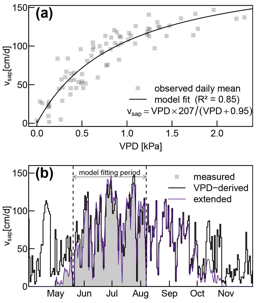
Figure A4(a) Relationship between daily mean values of vapor pressure deficit (VPD) and sap flow velocity (vsap). (b) Time series of measured and VPD-derived daily mean vsap. The model fitting period excludes the time before completion of leaf flush. The purple line shows the extended data as used for the xylem water age computations (values before April and after November are also 0).

Figure A5Input data for further RWU computations: spatially and temporally interpolated time series of (a) volumetric soil moisture, (b) soil δ18O and (c) soil δD. Vertical bars represent actual observations obtained by soil core measurements, and horizontal bars represent observations measured with probes.
A2 Post-processing of in situ measurements
A2.1 H2O ppmV correction
Following the volumetric moisture correction procedure described in Sect. 2.3, the relationship between volumetric sample moisture and the raw vapor δ18O and δD for both standards are shown in Fig. A2a and b, respectively. We split the whole data set into shorter periods (as indicated in Fig. A2c and d in order to check the consistency of this correction procedure. Two periods are striking: the first period (22 May 2019 to 1 June 2019) exhibits a lot of scatter for the heavy standards' δ18O values and also shows a strikingly high slope for the δD values. The second striking period is the fifth period (3 July 2019 to 11 July 2019) and coincides with the interrupted gas supply described in Sect. 3.1.4. Here, the slopes for δ18O are higher, and there is a clear negative offset of the δD values compared to all other periods. Over all of the seven sub-periods and both standard probes, the slope for δ18O ranges from to with a mean of (all values in ‰ ppmV−1), and the slope for δD lies between and with a mean value of (also all values in ‰ ppmV−1). Despite this notable spread of slopes, it turned out that the differences between the utilization of one (overall mean) slope for the moisture correction over the whole experiment does not lead to big differences compared to the utilization of period-specific slopes.
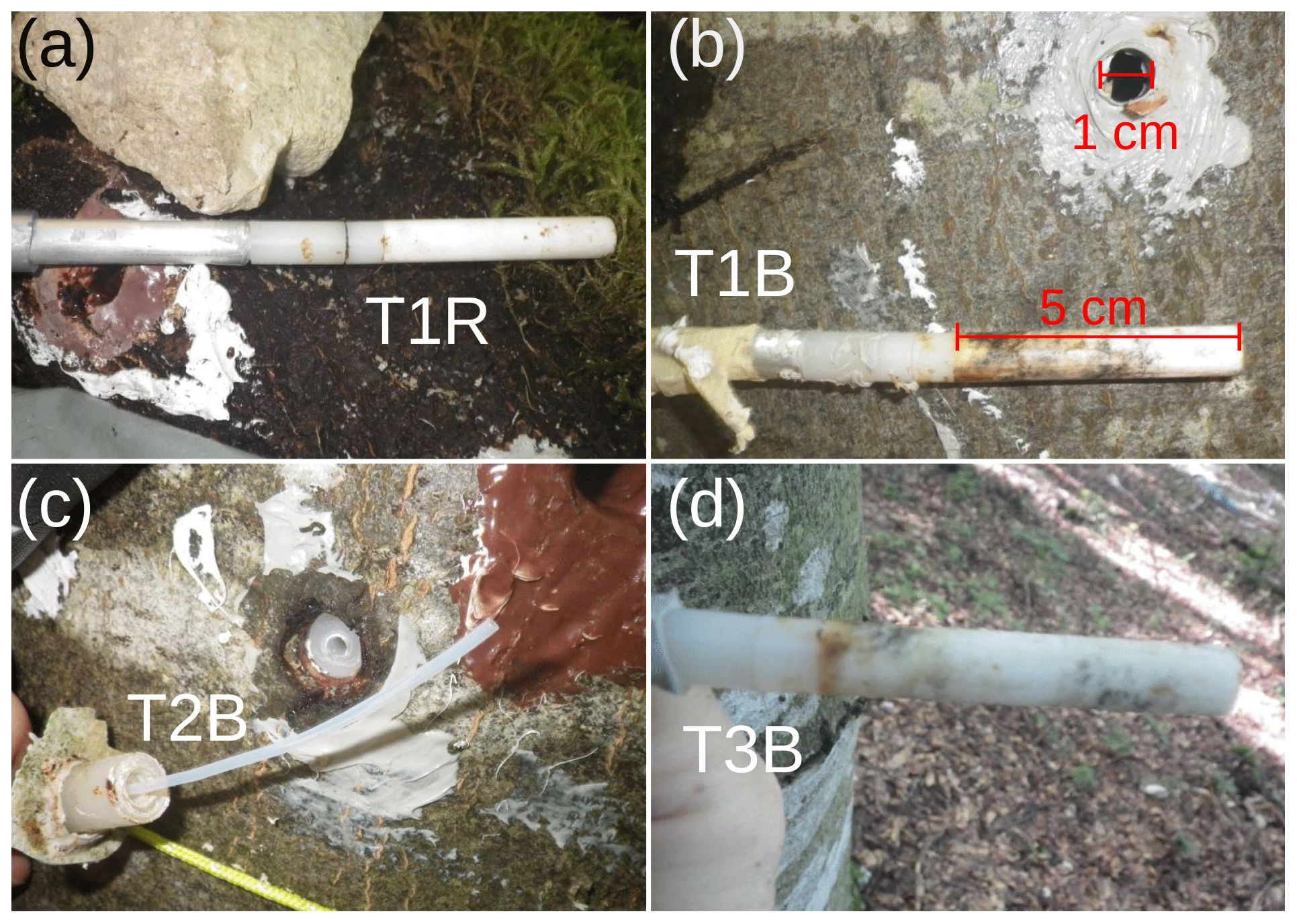
Figure A6Freshly removed XWIPs 12 weeks after installation. The heads of XWIPs T1B (b) and T3B (d) were covered with biofilms, while the head of T1R (a) was as good as new. During removal, the probe head of T2B (c) broke off. Callus formation around the drill hole already started.
A2.2 Manual data corrections
In terms of δ18O, three XWIPs (T1B, T2B and specifically T3B) exhibited similar dynamics in their time series compared to the remaining XWIPs (T1R, T1H, T2R and T2H), but seemed to have a negative offset, without any corresponding offset in their δD time series (Fig. A1a and b). Figure A3a shows all measurement values after moisture correction and normalization to the liquid phase. Assuming no further sources of water uptake than the observed soil profile and no fractionation during root water uptake, all of the xylem measurements (green, yellow and pink symbols) in Fig. A3a should be located within the green triangle of possible mixtures of soil water signatures (blue circles). The pink shaded area roughly marks the plot region containing implausible (i.e., impossible to achieve by soil water mixing) xylem water signatures. The values of T2R below the global meteoric water line (right half of Fig. A3a) fall into the time with interrupted gas supply (see Fig. A1) and were completely discarded. The XWIP values at the lower center of the plot fall into the starting period of the time series and are close to the values measured within the soil cores taken before the irrigation. The XWIP values to the left are the ones mentioned earlier (same dynamics, negative δ18O offset). We shifted these values into the plausible range by manually offsetting their δ18O time series until they fell into our mixing triangle. For T1B we added 2.5 ‰ to all values, and for T2B we added 1.5 ‰ starting at 1 June and another 0.5 ‰ starting from 11 July. For T3B we added 3.75 ‰ to all values and an additional 2 ‰ starting at 22 June.
The Supplement contains the code that can be used to reproduce the results of the paper.
The data needed to reproduce the paper results are contained within the Supplement.
The Supplement to this study contains the processed WIP measurements and all the climate, sap flow and soil moisture data needed to reproduce the essential results presented in this article. Furthermore, the Supplement contains R scripts that recreate the 2-D interpolation of soil moisture and isotopes (S1_soilInterpolation.r), the computation of δRWU (S2_XWIPs_and_RWU.r), the time series transformation and convolution of isotopic data (S3_transformation_and_convolution.r) and the computation of xylem water age distributions (S4_xylem_water_age.r). The supplement related to this article is available online at: https://doi.org/10.5194/bg-18-4603-2021-supplement.
SS and MW designed the experiment. SS conducted the fieldwork and data analysis and wrote the first draft. MW contributed to writing the final manuscript.
Markus Weiler is an inventor on German patent DE201310013969, which covers the probe technology. Stefan Seeger declares no competing interests.
Publisher's note: Copernicus Publications remains neutral with regard to jurisdictional claims in published maps and institutional affiliations.
Preparation and realization of the irrigation as well as parts of the probe installation were done by Britta Kattenstroth, Jonas Schwarz and Michael Rinderer. We would like to thank the reviewers John Marshall and Nicolas Brüggemann whose critical comments and suggestions helped to clarify and improve the manuscript.
This research has been supported by the Deutsche Forschungsgemeinschaft (grant no. SPP 1685).
This paper was edited by Andreas Ibrom and reviewed by John Marshall and Nicolas Brüggemann.
Badamasi, Y. A.: The working principle of an Arduino, in: 2014 11th International Conference on Electronics, Computer and Computation (ICECCO), IEEE, 1–4, 29 September–1 October 2014, Abuja, Nigeria, https://doi.org/10.1109/ICECCO.2014.6997578, 2014. a
Bernacchi, C. J. and VanLoocke, A.: Terrestrial Ecosystems in a Changing Environment: A Dominant Role for Water, Annu. Revi. Plant Biol., 66, 599–622, https://doi.org/10.1146/annurev-arplant-043014-114834, 2015. a
Beyer, M., Kühnhammer, K., and Dubbert, M.: In situ measurements of soil and plant water isotopes: a review of approaches, practical considerations and a vision for the future, Hydrol. Earth Syst. Sci., 24, 4413–4440, https://doi.org/10.5194/hess-24-4413-2020, 2020. a, b, c
Brinkmann, N., Seeger, S., Weiler, M., Buchmann, N., Eugster, W., and Kahmen, A.: Employing stable isotopes to determine the residence times of soil water and the temporal origin of water taken up by Fagus sylvatica and Picea abies in a temperate forest, New Phytol., 219, 1300–1313, https://doi.org/10.1111/nph.15255, 2018. a, b, c
Busch, D. E., Ingraham, N. L., and Smith, S. D.: Water Uptake in Woody Riparian Phreatophytes of the Southwestern United States: A Stable Isotope Study, Ecol. Appl., 2, 450–459, https://doi.org/10.2307/1941880, 1992. a
Calder, I. R.: Implications and assumptions in using the `total counts' and convection-dispersion equations for tracer flow measurements – With particular reference to transpiration measurements in trees, J. Hydrol., 125, 149–158, https://doi.org/10.1016/0022-1694(91)90088-Y, 1991. a
Campbell, G. S., Calissendorff, C., and Williams, J. H.: Probe for Measuring Soil Specific Heat Using A Heat-Pulse Method, Soil Sci. Soc. Am. J., 55, 291–293, https://doi.org/10.2136/sssaj1991.03615995005500010052x, 1991. a
Chang, E., Wolf, A., Gerlein-Safdi, C., and Caylor, K. K.: Improved removal of volatile organic compounds for laser-based spectroscopy of water isotopes, Rapid Commun. Mass Sp., 30, 784–790, https://doi.org/10.1002/rcm.7497, 2016. a
Dalton, F. N.: Plant root water extraction studies using stable isotopes, Plant Soil, 111, 217–221, https://doi.org/10.1007/BF02139942, 1988. a
Dawson, T. E. and Ehleringer, J. R.: Streamside trees that do not use stream water, Nature, 350, 335–337, https://doi.org/10.1038/350335a0, 1991. a, b
Dawson, T. E., Mambelli, S., Plamboeck, A. H., Templer, P. H., and Tu, K. P.: Stable Isotopes in Plant Ecology, Annu. Rev. Ecol. Syst., 33, 507–559, https://doi.org/10.1146/annurev.ecolsys.33.020602.095451, 2002. a
De Deurwaerder, H. P. T., Visser, M. D., Detto, M., Boeckx, P., Meunier, F., Kuehnhammer, K., Magh, R.-K., Marshall, J. D., Wang, L., Zhao, L., and Verbeeck, H.: Causes and consequences of pronounced variation in the isotope composition of plant xylem water, Biogeosciences, 17, 4853–4870, https://doi.org/10.5194/bg-17-4853-2020, 2020. a, b, c, d, e
Derby, R. W. and Gates, D. M.: The Temperature of Tree Trunks-Calculated and Observed, Am. J. Bot., 53, 580, https://doi.org/10.1002/j.1537-2197.1966.tb07374.x, 1966. a
Ehleringer, J. R. and Dawson, T. E.: Water uptake by plants: perspectives from stable isotope composition, Plant Cell Environ., 15, 1073–1082, https://doi.org/10.1111/j.1365-3040.1992.tb01657.x, 1992. a
Evaristo, J., Kim, M., van Haren, J., Pangle, L. A., Harman, C. J., Troch, P. A., and McDonnell, J. J.: Characterizing the Fluxes and Age Distribution of Soil Water, Plant Water, and Deep Percolation in a Model Tropical Ecosystem, Water Resour. Res., 55, 3307–3327, https://doi.org/10.1029/2018WR023265, 2019. a, b
Feddes, R. A., Kowalik, P., Kolinska-Malinka, K., and Zaradny, H.: Simulation of field water uptake by plants using a soil water dependent root extraction function, J. Hydrol., 31, 13–26, https://doi.org/10.1016/0022-1694(76)90017-2, 1976. a, b
Gaines, K. P., Meinzer, F. C., Duffy, C. J., Thomas, E. M., and Eissenstat, D. M.: Rapid tree water transport and residence times in a Pennsylvania catchment, Ecohydrology, 9, 1554–1565, https://doi.org/10.1002/eco.1747, 2016. a, b, c, d, e
Gaj, M., Beyer, M., Koeniger, P., Wanke, H., Hamutoko, J., and Himmelsbach, T.: In situ unsaturated zone water stable isotope (2H and 18O) measurements in semi-arid environments: a soil water balance, Hydrol. Earth Syst. Sci., 20, 715–731, https://doi.org/10.5194/hess-20-715-2016, 2016. a
Gaj, M., Kaufhold, S., Koeniger, P., Beyer, M., Weiler, M., and Himmelsbach, T.: Mineral mediated isotope fractionation of soil water, Rapid Commun. Mass Sp., 31, 269–280, https://doi.org/10.1002/rcm.7787, 2017. a
Garvelmann, J., Külls, C., and Weiler, M.: A porewater-based stable isotope approach for the investigation of subsurface hydrological processes, Hydrol. Earth Syst. Sci., 16, 631–640, https://doi.org/10.5194/hess-16-631-2012, 2012. a
Gebauer, T., Horna, V., and Leuschner, C.: Variability in radial sap flux density patterns and sapwood area among seven co-occurring temperate broad-leaved tree species, Tree Physiol., 28, 1821–1830, https://doi.org/10.1093/treephys/28.12.1821, 2008. a
Gerwitz, A. and Page, E. R.: An Empirical Mathematical Model to Describe Plant Root Systems, J. Appl. Ecol., 11, 773, https://doi.org/10.2307/2402227, 1974. a
Goldsmith, G. R., Allen, S. T., Braun, S., Engbersen, N., González-Quijano, C. R., Kirchner, J. W., and Siegwolf, R. T.: Spatial variation in throughfall, soil, and plant water isotopes in a temperate forest, Ecohydrology, 12, 1–11, https://doi.org/10.1002/eco.2059, 2019. a
Gralher, B., Herbstritt, B., Weiler, M., Wassenaar, L. I., and Stumpp, C.: Correcting for Biogenic Gas Matrix Effects on Laser-Based Pore Water-Vapor Stable Isotope Measurements, Vadose Zone J., 17, 170157, https://doi.org/10.2136/vzj2017.08.0157, 2018. a
Guderle, M. and Hildebrandt, A.: Using measured soil water contents to estimate evapotranspiration and root water uptake profiles – a comparative study, Hydrol. Earth Syst. Sci., 19, 409–425, https://doi.org/10.5194/hess-19-409-2015, 2015. a
Hassler, S. K., Weiler, M., and Blume, T.: Tree-, stand- and site-specific controls on landscape-scale patterns of transpiration, Hydrol. Earth Syst. Sci., 22, 13–30, https://doi.org/10.5194/hess-22-13-2018, 2018. a, b
James, S. A., Meinzer, F. C., Goldstein, G., Woodruff, D., Jones, T., Restom, T., Mejia, M., Clearwater, M., and Campanello, P.: Axial and radial water transport and internal water storage in tropical forest canopy trees, Oecologia, 134, 37–45, https://doi.org/10.1007/s00442-002-1080-8, 2003. a, b, c
Jarvis, N.: A simple empirical model of root water uptake, J. Hydrol., 107, 57–72, https://doi.org/10.1016/0022-1694(89)90050-4, 1989. a, b, c, d, e
Kirchner, J. W., Feng, X., and Neal, C.: Fractal stream chemistry and its implications for contaminant transport in catchments, Nature, 403, 524–527, https://doi.org/10.1038/35000537, 2000. a
Knighton, J., Kuppel, S., Smith, A., Soulsby, C., Sprenger, M., and Tetzlaff, D.: Using isotopes to incorporate tree water storage and mixing dynamics into a distributed ecohydrologic modelling framework, Ecohydrology, 13, e2201, https://doi.org/10.1002/eco.2201, 2020. a, b, c, d, e
Kübert, A., Paulus, S., Dahlmann, A., Werner, C., Rothfuss, Y., Orlowski, N., and Dubbert, M.: Water Stable Isotopes in Ecohydrological Field Research: Comparison Between In Situ and Destructive Monitoring Methods to Determine Soil Water Isotopic Signatures, Front. Plant Sci., 11, 1–13, https://doi.org/10.3389/fpls.2020.00387, 2020. a, b
Lv, L.: Linking Montane Soil Moisture Measurements to Evapo- transpiration Using Inverse Numerical Modeling, Ph.D. thesis, Utah State University, Logan, Utah, available at: https://digitalcommons.usu.edu/etd/3323 (last access: 9 July 2021), 2014. a
Magh, R. K., Eiferle, C., Burzlaff, T., Dannenmann, M., Rennenberg, H., and Dubbert, M.: Competition for water rather than facilitation in mixed beech-fir forests after drying-wetting cycle, J. Hydrol., 587, 124944, https://doi.org/10.1016/j.jhydrol.2020.124944, 2020. a, b, c
Majoube, M.: Fractionnement en oxygène 18 et en deutérium entre l'eau et sa vapeur, J. Chim. Phys., 68, 1423–1436, https://doi.org/10.1051/jcp/1971681423, 1971. a
Małoszewski, P. and Zuber, A.: Determining the turnover time of groundwater systems with the aid of environmental tracers, J. Hydrol., 57, 207–231, 1982. a
Marshall, J. D., Cuntz, M., Beyer, M., Dubbert, M., and Kuehnhammer, K.: Borehole Equilibration: Testing a New Method to Monitor the Isotopic Composition of Tree Xylem Water in situ, Front. Plant Sci., 11, 1–14, https://doi.org/10.3389/fpls.2020.00358, 2020. a, b, c, d, e
McGuire, K. J. and McDonnell, J. J.: A review and evaluation of catchment transit time modeling, J. Hydrol., 330, 543–563, https://doi.org/10.1016/j.jhydrol.2006.04.020, 2006. a
Meinzer, F. C., Brooks, J. R., Domec, J. C., Gartner, B. L., Warren, J. M., Woodruff, D. R., Bible, K., and Shaw, D. C.: Dynamics of water transport and storage in conifers studied with deuterium and heat tracing techniques, Plant Cell Environ., 29, 105–114, https://doi.org/10.1111/j.1365-3040.2005.01404.x, 2006. a, b, c, d, e, f, g, h
Newberry, S. L., Nelson, D. B., and Kahmen, A.: Cryogenic vacuum artifacts do not affect plant water-uptake studies using stable isotope analysis, Ecohydrology, 10, 1–10, https://doi.org/10.1002/eco.1892, 2017. a
Oerter, E. J. and Bowen, G.: In situ monitoring of H and O stable isotopes in soil water reveals ecohydrologic dynamics in managed soil systems, Ecohydrology, 10, 1–13, https://doi.org/10.1002/eco.1841, 2017. a, b
Orlowski, N., Frede, H.-G., Brüggemann, N., and Breuer, L.: Validation and application of a cryogenic vacuum extraction system for soil and plant water extraction for isotope analysis, J. Sens. Sens. Syst., 2, 179–193, https://doi.org/10.5194/jsss-2-179-2013, 2013. a
Orlowski, N., Pratt, D. L., and McDonnell, J. J.: Intercomparison of soil pore water extraction methods for stable isotope analysis, Hydrol. Process., 30, 3434–3449, https://doi.org/10.1002/hyp.10870, 2016. a
Rabbel, I., Bogena, H., Neuwirth, B., and Diekkrüger, B.: Using sap flow data to parameterize the feddes water stress model for Norway spruce, Water-Sui., 10, 279, https://doi.org/10.3390/w10030279, 2018. a
Rennenberg, H., Schneider, S., and Weber, P.: Analysis of uptake and allocation of nitrogen and sulphur compounds by trees in the field, J. Exp. Bot., 47, 1491–1498, https://doi.org/10.1093/jxb/47.10.1491, 1996. a
Rothfuss, Y. and Javaux, M.: Reviews and syntheses: Isotopic approaches to quantify root water uptake: a review and comparison of methods, Biogeosciences, 14, 2199–2224, https://doi.org/10.5194/bg-14-2199-2017, 2017. a
Rothfuss, Y., Vereecken, H., and Brüggemann, N.: Monitoring water stable isotopic composition in soils using gas-permeable tubing and infrared laser absorption spectroscopy, Water Resour. Res., 49, 3747–3755, https://doi.org/10.1002/wrcr.20311, 2013. a, b, c, d, e
Rothfuss, Y., Merz, S., Vanderborght, J., Hermes, N., Weuthen, A., Pohlmeier, A., Vereecken, H., and Brüggemann, N.: Long-term and high-frequency non-destructive monitoring of water stable isotope profiles in an evaporating soil column, Hydrol. Earth Syst. Sci., 19, 4067–4080, https://doi.org/10.5194/hess-19-4067-2015, 2015. a
Scholander, P. F., Hammel, H. T., Bradstreet, E. D., and Hemmingsen, E. A.: Sap pressure in vascular plants, Science, 148, 339–346, https://doi.org/10.1126/science.148.3668.339, 1965. a
Schwendenmann, L., Dierick, D., Köhler, M., and Hölscher, D.: Can deuterium tracing be used for reliably estimating water use of tropical trees and bamboo?, Tree Physiol., 30, 886–900, https://doi.org/10.1093/treephys/tpq045, 2010. a, b, c, d, e
Šimůnek, J., van Genuchten, M. T., and Šejna, M.: Development and Applications of the HYDRUS and STANMOD Software Packages and Related Codes, Vadose Zone J., 7, 587–600, https://doi.org/10.2136/vzj2007.0077, 2008. a
Soderberg, K., Good, S. P., Wang, L., and Caylor, K.: Stable Isotopes of Water Vapor in the Vadose Zone: A Review of Measurement and Modeling Techniques, Vadose Zone J., 11, vzj2011.0165, https://doi.org/10.2136/vzj2011.0165, 2012. a
Sprenger, M., Seeger, S., Blume, T., and Weiler, M.: Travel times in the vadose zone: Variability in space and time, Water Resour. Res., 52, 5727–5754, https://doi.org/10.1002/2015WR018077, 2016. a
Sprenger, M., Stumpp, C., Weiler, M., Aeschbach, W., Allen, S. T., Benettin, P., Dubbert, M., Hartmann, A., Hrachowitz, M., Kirchner, J. W., McDonnell, J. J., Orlowski, N., Penna, D., Pfahl, S., Rinderer, M., Rodriguez, N., Schmidt, M., and Werner, C.: The Demographics of Water: A Review of Water Ages in the Critical Zone, Rev. Geophys., 57, 800–834, https://doi.org/10.1029/2018RG000633, 2019. a
Steppe, K., De Pauw, D. J., Doody, T. M., and Teskey, R. O.: A comparison of sap flux density using thermal dissipation, heat pulse velocity and heat field deformation methods, Agr. Forest Meteorol., 150, 1046–1056, https://doi.org/10.1016/j.agrformet.2010.04.004, 2010. a, b, c
Stumpp, C., Stichler, W., Kandolf, M., and Šimůnek, J.: Effects of Land Cover and Fertilization Method on Water Flow and Solute Transport in Five Lysimeters: A Long-Term Study Using Stable Water Isotopes, Vadose Zone J., 11, 1–14, https://doi.org/10.2136/vzj2011.0075, 2012. a
Urban, J., Bednárová, E., Plichta, R., Gryc, V., Vavrčík, H., Hacura, J., Fajstavr, M., and Kučera, J.: Links between phenology and ecophysiology in a European beech forest, IForest, 8, 438–447, https://doi.org/10.3832/ifor1307-007, 2015. a
van Meerveld, H. J. I., Kirchner, J. W., Vis, M. J. P., Assendelft, R. S., and Seibert, J.: Expansion and contraction of the flowing stream network alter hillslope flowpath lengths and the shape of the travel time distribution, Hydrol. Earth Syst. Sci., 23, 4825–4834, https://doi.org/10.5194/hess-23-4825-2019, 2019. a
Volkmann, T. H. M. and Weiler, M.: Continual in situ monitoring of pore water stable isotopes in the subsurface, Hydrol. Earth Syst. Sci., 18, 1819–1833, https://doi.org/10.5194/hess-18-1819-2014, 2014. a, b, c, d, e, f, g
Volkmann, T. H. M., Haberer, K., Gessler, A., and Weiler, M.: High-resolution isotope measurements resolve rapid ecohydrological dynamics at the soil-plant interface, New Phytol., 210, 839–849, https://doi.org/10.1111/nph.13868, 2016a. a, b, c
Volkmann, T. H. M., Kühnhammer, K., Herbstritt, B., Gessler, A., and Weiler, M.: A method for in situ monitoring of the isotope composition of tree xylem water using laser spectroscopy, Plant Cell Environ., 39, 2055–2063, https://doi.org/10.1111/pce.12725, 2016b. a, b, c
Wassenaar, L. I., Hendry, M., Chostner, V., and Lis, G.: High Resolution Pore Water δ2H and δ18O Measurements by H2O(liquid)–H2O(vapor) Equilibration Laser Spectroscopy, Environ. Sci. Technol., 42, 9262–9267, https://doi.org/10.1021/es802065s, 2008. a
Weiler, M., McGlynn, B. L., McGuire, K. J., and McDonnell, J. J.: How does rainfall become runoff? A combined tracer and runoff transfer function approach, Water Resour. Res., 39, 1315, https://doi.org/10.1029/2003WR002331, 2003. a
West, A. G., Goldsmith, G. R., Brooks, P. D., and Dawson, T. E.: Discrepancies between isotope ratio infrared spectroscopy and isotope ratio mass spectrometry for the stable isotope analysis of plant and soil waters, Rapid Commun. Mass Sp., 24, 1948–1954, https://doi.org/10.1002/rcm.4597, 2010. a
White, J. W., Cook, E. R., Lawrence, J. R., and Wallace S., B.: The DH ratios of sap in trees: Implications for water sources and tree ring DH ratios, Geochim. Cosmochim. Ac., 49, 237–246, https://doi.org/10.1016/0016-7037(85)90207-8, 1985. a
Yepez, E. a., Huxman, T. E., Ignace, D. D., English, N. B., Weltzin, J. F., Castellanos, A. E., and Williams, D. G.: Dynamics of transpiration and evaporation following a moisture pulse in semiarid grassland: A chamber-based isotope method for partitioning flux components, Agr. Forest Meteorol., 132, 359–376, https://doi.org/10.1016/j.agrformet.2005.09.006, 2005. a
Zhang, L., Dawes, W., Slavich, P., Meyer, W., Thorburn, P. J., Smith, D., and Walker, G.: Growth and ground water uptake responses of lucerne to changes in groundwater levels and salinity: Lysimeter, isotope and modelling studies, Agr. Water Manage., 39, 265–282, https://doi.org/10.1016/S0378-3774(98)00082-1, 1999. a