the Creative Commons Attribution 4.0 License.
the Creative Commons Attribution 4.0 License.
 | 17 Aug 2021
Carbon balance of a Finnish bog: temporal variability and limiting factors based on 6 years of eddy-covariance data
Pavel Alekseychik
Aino Korrensalo
Ivan Mammarella
Samuli Launiainen
Eeva-Stiina Tuittila
Ilkka Korpela
Timo Vesala
Pristine boreal mires are known as substantial sinks of carbon dioxide (CO2) and net emitters of methane (CH4). Bogs constitute a major fraction of pristine boreal mires. However, the bog CO2 and CH4 balances are poorly known, having been largely estimated based on discrete and short-term measurements by manual chambers and seldom using the eddy-covariance (EC) technique.
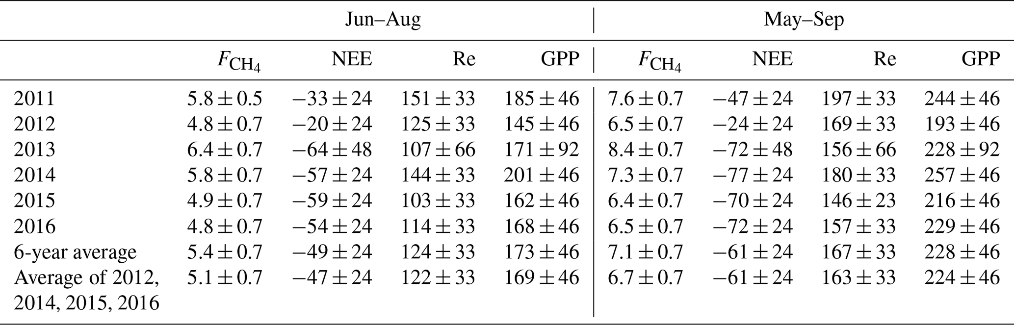
Eddy-covariance (EC) measurements of CO2 and CH4 exchange were conducted in the Siikaneva mire complex in southern Finland in 2011–2016. The site is a patterned bog having a moss–sedge–shrub vegetation typical of southern Eurasian taiga, with several ponds near the EC tower. The study presents a complete series of CO2 and CH4 EC flux () measurements and identifies the environmental factors controlling the ecosystem–atmosphere CO2 and CH4 exchange. A 6-year average growing season (May–September) cumulative CO2 exchange of −61 ± 24 g C m−2 was observed, which partitions into mean total respiration (Re) of 167 ± 33 (interannual range 146–197) g C m−2 and mean gross primary production (GPP) of 228 ± 46 (interannual range 193–257) g C m−2, while the corresponding amounts to 7.1 ± 0.7 (interannual range 6.4–8.4) g C m−2. The contribution of October–December CO2 and CH4 fluxes to the cumulative sums was not negligible based on the measurements during one winter.
GPP, Re and increased with temperature. GPP and did not show any significant decline even after a substantial water table drawdown in 2011. Instead, GPP, Re and were limited in the cool, cloudy and wet growing season of 2012. May–September cumulative net ecosystem exchange (NEE) of 2013–2016 averaged at about −73 g C m−2, in contrast with the hot and dry year 2011 and the wet and cool year 2012. Suboptimal weather likely reduced the net sink by about 25 g C m−2 in 2011 due to elevated Re, and by about 40 g C m−2 in 2012 due to limited GPP. The cumulative growing season sums of GPP and CH4 emission showed a strong positive relationship.
The EC source area was found to be comprised of eight distinct surface types. However, footprint analyses revealed that contributions of different surface types varied only within 10 %–20 % with respect to wind direction and stability conditions. Consequently, no clear link between CO2 and CH4 fluxes and the EC footprint composition was found despite the apparent variation in fluxes with wind direction.
- Article
(13141 KB) - Full-text XML
- BibTeX
- EndNote


Natural mires are an important element of the boreal and Arctic carbon cycle due to the vast amounts of carbon stored in peat and their sensitivity to environmental changes (Gorham, 1991; Charman et al., 2013). Over the last 10–14 thousand years, the northern mires have provided substantial climatic cooling (Frolking and Roulet, 2007). It is expected, however, that the rising air temperature will likely drive an increase in the emission of methane (CH4) (Zhang et al., 2017) and carbon dioxide (CO2) (Laine et al. 2019). As the effects of rising temperature are strongly dependent on water table level (Davidson and Janssens, 2006; Buttler et al., 2015; Laine et al. 2019), the precipitation extremes in northern latitudes (IPCC 2013) will contribute to the variability and uncertainty of any predictions.
Pristine bogs, i.e. primarily rain-fed, oligotrophic peatlands with a developed microtopography and often populated by trees, constitute a major and diverse class of boreal mires (Seppä 2002). The response of their greenhouse gas (GHG) balances to the environment is therefore of utmost interest. The complex surface patterning of a bog and the need for continuous measurements favor the application of area-integrating eddy-covariance (EC) measurements (Baldocchi, 2008), a technique providing an estimate of vertical net flux of scalars and heat over a large (∼ 1–100 ha) source–sink area (flux footprint) that typically envelops all representative microsites. However, most boreal bog GHG balance estimates to date have been produced using flux chambers (Bubier et al., 1993; Alm et al., 1999a, b; Waddington and Roulet, 2000; Bubier et al., 2003; Laine et al., 2006; Saarnio et al., 2007; Korrensalo et al., 2019), which requires ecological understanding of the spatial variability of a strongly patterned ecosystem for reliable upscaling (Laine et al., 2009; Riutta et al., 2007), which requires very labor-intensive and lengthy field campaigns. Therefore, it would be of high interest to examine a multiannual EC record from a bog site.
The strong ecological diversity of bogs is reflected in previous bog eddy-covariance studies, which examined a temperate wooded bog (Fäjemyr; Lund et al., 2007, 2012), temperate shrub bog (Mer Bleu; Lafleur et al., 2001, 2005; Roulet et al., 2007; Brown, 2014), boreal treed/low shrub bog (Attawapiskat river; Humphreys et al., 2014), boreal shrub bog (Kinoje Lake; Humphreys et al., 2014), boreal raised bog (Tchebakova et al., 2015), boreal collapse scar bog (Bonanza Creek Experimental Forest; Euskirchen et al., 2014), boreal raised patterned bog (Mukhrino; Alekseychik et al., 2017), temperate patterned Sphagnum–shrub bog (Arneth et al., 2002), and boreal open patterned bog (Arneth et al., 2002). Due to such a broad range of vegetation and climate, identifying the “typical” bog GHG balance and its environmental controls presents a certain challenge.
The previous EC and chamber estimates indicate that boreal bogs typically demonstrate a small to moderate annual sink of CO2 and a relatively small source of CH4, with the flux rates being similar to those observed in fens. Net loss of carbon has been observed in exceptionally dry summers (Alm et al., 1999a; Waddington and Roulet, 2000). The annual (or growing season) net CO2 exchange in bogs across the entire boreal region typically varies from +30 to −100 (e.g. Alm et al., 1999a; Waddington and Roulet, 2000; Bubier et al., 2003; Laine et al., 2006; Saarnio et al., 2007; Tchebakova et al., 2015; Lund et al., 2010; Roulet et al., 2007; Lafleur et al. 2003; Korrensalo et al., 2019), which splits into gross primary productivity (GPP) and ecosystem respiration (Re) both typically in the range of 200–500 . The fairly wide spread in these numbers is attributed to the variation in site-specific (vegetation, hydrology, peat structure; see Moore et al., 2002 and Korrensalo et al., 2018, for dry and wet bog, respectively) and external (climate, weather; Moore et al., 2002; and Laine et al., 2006, for continental and maritime bog, respectively) factors. Studies extending over several years reveal that bog CO2 balance is sensitive to temperature and water table level (WTD) (Lafleur et al., 2003; Rinne et al., 2020). Hot and dry weather suppresses bog photosynthesis and promotes respiration (Alm et al., 1999a; Lund et al., 2012; Euskirchen et al., 2014; Arneth et al., 2002; Tchebakova et al., 2015). Under favorable conditions, which seem to consist of warm temperatures, ample sunshine, sufficient moisture but no long-term WTD rise, bogs can show a high growing season net CO2 uptake of 100–200 g C m−2 (e.g. Friborg et al., 2003; Alekseychik et al., 2017).
In wetlands, the total methane emission is a sum of diffusion through soil matrix, ebullition and plant transport, each associated with a set of environmental controls (Lai, 2009; Dorodnikov, 2011; Ström et al., 2015; Korrensalo, 2018; Männistö et al., 2019; Riutta et al., 2020). Peat temperature is known to be the primary driver of CH4 production (e.g. Dunfield et al., 1993). About 50 %–90 % of the produced methane is oxidized in the oxic zone before it can reach the atmosphere (King et al., 1990; Fenchner and Hemond, 1992; Whalen and Reeburgh, 2000), so WTD is a priori an important driver. While wet surfaces were considered to be the highest emitters (Bubier et al., 2005), recent work has shown the maximum fluxes to occur at intermediate WTD microsites (Turetsky et al., 2014; Rinne et al. 2018). There contradictions call for multiyear studies from patterned bogs to reveal the temporal controls of methane emissions.
At present, the lack of multi-year eddy-covariance studies in boreal bogs does not allow us to rank the environmental controls by their importance for CH4 emission. It was previously observed that northern bogs typically emit from 0 to 20 g C m−2 annually in the form of methane (Vompersky et al., 2000; Friborg et al., 2003; Roulet et al., 2007). The bogs with developed ridge–hollow microtopography were identified as the mire types with the highest CH4 emission spatial variability in western Siberia (Kalyuzhny et al., 2009); a high spatial heterogeneity was also found in a Canadian bog study (Moore et al., 2011).
The available shorter datasets from bogs, and the more abundant data from fens, do shed some light on the possible controls. Methane net efflux () is strongly correlated with GPP; to which extent this is due to accelerated rhizospheric CH4 production as a result of photosynthate input or enhancement of CH4 transport by vascular plants is not clear (Bellisario et al., 1999; Rinne et al., 2018). The WTD control is equally unclear, with reports of both an optimum WTD (e.g. Rinne et al., 2018) and a limitation in CH4 efflux at WTD drawdown (Glagolev et al., 2001; Kalyuzhny et al., 2009). Euskirchen et al. (2014) show that only a drought or considerable strength is able to limit bog CH4 emission. CH4 ebullition is prompted by drops in atmospheric pressure but is reduced by drops in peat temperature (Fechner-Levy and Hemond, 1996).
The EC technique is usually assumed to provide flux estimates representative of the studied ecosystem (e.g. Aubinet et al., 2012). However, in heterogeneous sites this may not be the case. The bog surface cover heterogeneity has several characteristic spatial scales, including vegetation community (1 m2); microsites, e.g. hummocks and hollows (1–10 m2); and larger formations, such as ponds and ridges (50–1000 m2). These surface elements have been shown to have significantly different surface–atmosphere GHG exchange rates (Alm et al., 1999a; Repo et al., 2007; Maksuytov et al., 2010; Kazantsev and Glagolev, 2010). In order to understand the output of an EC system in such a heterogeneous site, one needs to estimate the contributions of the surface cover types to the total flux. Due to the specifics of atmospheric transport, the EC flux is strongly influenced by sources close to the EC tower (Vesala et al., 2008), but also by the larger-scale general surface composition in different wind direction sectors. The possible effect of the resulting footprint variation on the EC data calls for detailed inquiry (e.g. Tuovinen et al., 2019).
In the present study, we report 6 years of CO2 and CH4 fluxes measured by EC at a raised patterned bog area of the Siikaneva mire, southern Finland. The long-term data are used to analyze the responses of bog–atmosphere CO2 and CH4 exchange to environmental forcing during the growing season (May–September) and to provide growing season balances. Specifically, we aim to
-
quantify CO2 and CH4 balances of a boreal bog ecosystem on seasonal and interannual timescales,
-
identify the environmental controls responsible for seasonal and interannual variability of bog carbon exchange,
-
inquire whether signals from surface heterogeneity within the footprint can be associated with the observed CO2 and CH4 fluxes.
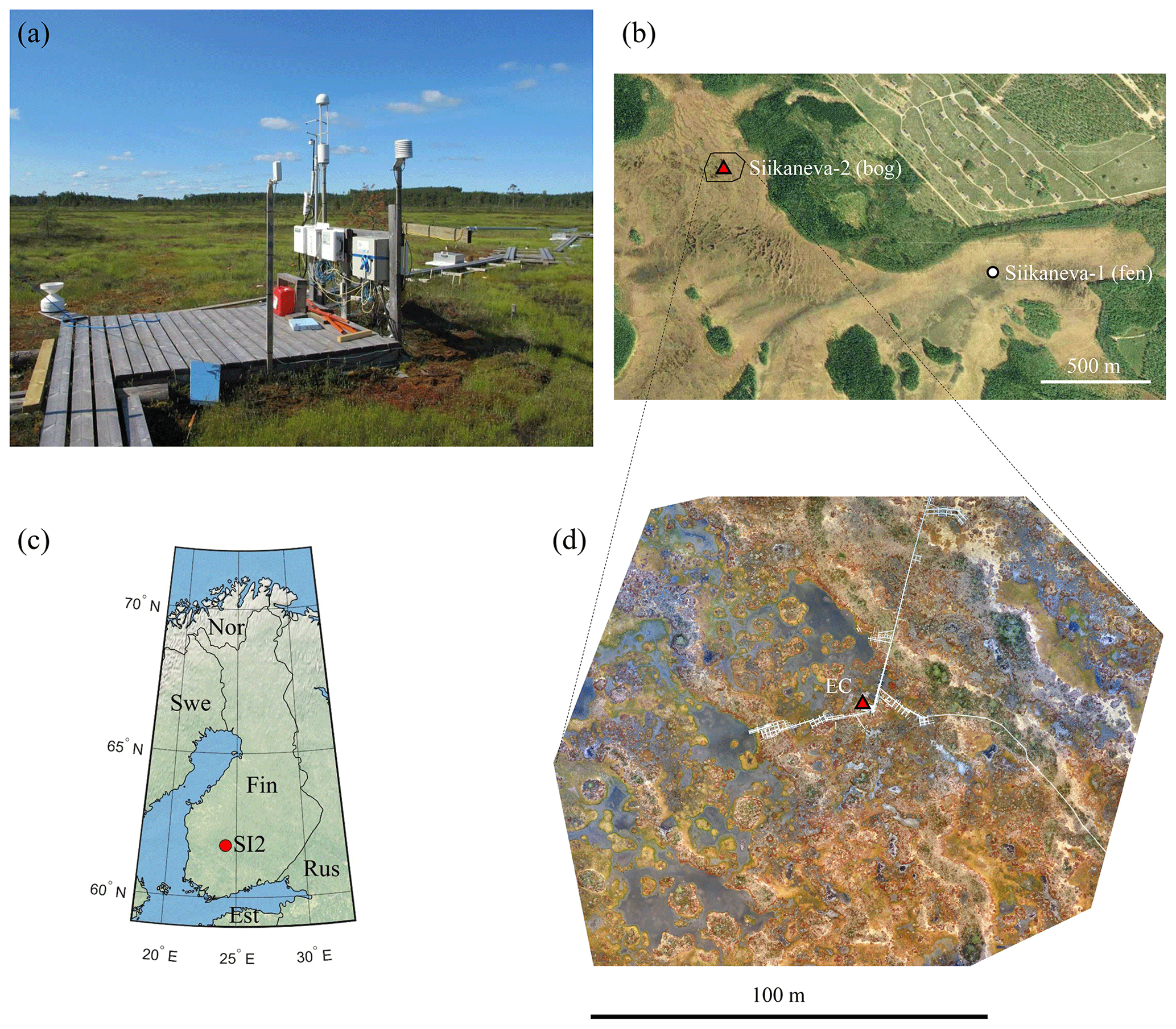
Figure 1(a) Photo of the eddy-covariance tower and meteorological setup facing southwest. (b) Map of the Siikaneva mire with the bog (SI2, this study) and fen (SI1, Rinne et al., 2018) sites marked. (c) Map of Finland showing the location of the Siikaneva-2 site. (d) Aerial RGB orthomosaic showing the main EC footprint contribution zone, based on the imagery obtained on 18 June 2018 during a dry period.
2.1 Site description and previous research
The Siikaneva-2 site (61.8∘ N, 24.2∘ E) is situated in a patterned ombrotrophic bog within the larger Siikaneva mire complex in southern Finland (Fig. 1). The microtopography is dominated by rows of hummock strings (Fig. 1a, b and d). The areas with lower elevation are considerably varied, being composed of hollows and lawns, moss-free mud bottoms, and ponds. The dominating moss species are Sphagnum rubellum, S. papillosum and S. fuscum, while the most widespread vascular plants are Rhynchospora alba, Andromeda polifolia, Calluna vulgaris and Rubus chamaemorus; a few small Scots pines (Pinus sylvestris) grow on the ridges.
The pond depths range from 0 to 2 m. The temporal variations in the bog water level lead to the variation in pond size and occasionally result in inundation of the mud bottoms. The 4-year average (2012–2015) peak total vascular plant leaf area index (LAI) was 0.35 m2 m−2, and the peak aerenchymatous LAI was 0.24 m2 m−2. Details on microform types and vegetation composition are given in Korrensalo et al. (2016) and Korrensalo et al. (2017).
The site is highly heterogeneous due to the patchy vegetation cover. The western sector of the EC footprint is dominated by ponds, hollows and lawns, while in the eastern sector one encounters several well-defined ridges (Fig. 1d). The nearest forest edge lies 150 m NE of the EC tower.
Table 1Fraction of 30 min EC fluxes of CO2 and CH4 remaining after the quality checks and u∗ filtering, in percent of the specified period.
2.2 Measurements
2.2.1 Eddy-covariance measurements
EC measurements of CO2, CH4, and sensible and latent heat fluxes were conducted at the site in the years 2011–2016 using a METEK USA-1 anemometer, a LiCor LI-7700 open-path CH4 analyzer, and a LiCor LI-7200 enclosed path CO2 and H2O analyzer mounted at 2.4 m height above the moss surface. The EC raw data were processed using EddyUH software (Mammarella et al., 2016) following standard schemes and quality control protocols (Nemitz et al., 2018; Sabbatini et al., 2018). The CH4 flux data at relative signal strength (RSSI) < 20 were excluded from analysis based on the regression of versus RSSI. A friction velocity (u∗) filter of 0.1 m s−1 was applied based on the observed behavior of the normalized CH4 and CO2 fluxes under low-turbulence conditions (Appendix A). See Table 1 for the proportion of the 30 min average CO2 and CH4 fluxes remaining after quality control and u∗ filtering. We conventionally define May–September as the growing season and October–April as the non-growing season.
2.2.2 Auxiliary measurements
Meteorological and environmental measurements were conducted next to the EC tower. Peat temperature (Tp) profile was measured by Campbell 107 Thermistor sensors at 5, 20, 35 and 50 cm depths starting in July 2011. In April 2012, the auxiliary measurements were expanded with a net radiation sensor Kipp and Zonen NR Lite2, air temperature (Ta) and relative humidity (RH) sensor Campbell CS215, WTD sensor Campbell CS451, and tipping bucket rain gauge ARG-100. The peat temperature profile and the water table sensor were installed in a lawn microform near the EC tower.
The peat temperature at 20 cm depth (Tp20) and WTD were gap-filled using regressions with the data from the Siikaneva-1 fen station (SI1, Rinne et al., 2007, 2018) 1.2 km SE from the site. Measurements from the SMEAR-II station (Hyytiälä, 7 km away) were used to gap-fill Ta and RH and supply the complete time series of photosynthetic active radiation (PAR). The precipitation rate time series was constructed as a combination of observations at the SMEAR-II site and Finnish Meteorological Institute weather station in Hyytiälä.
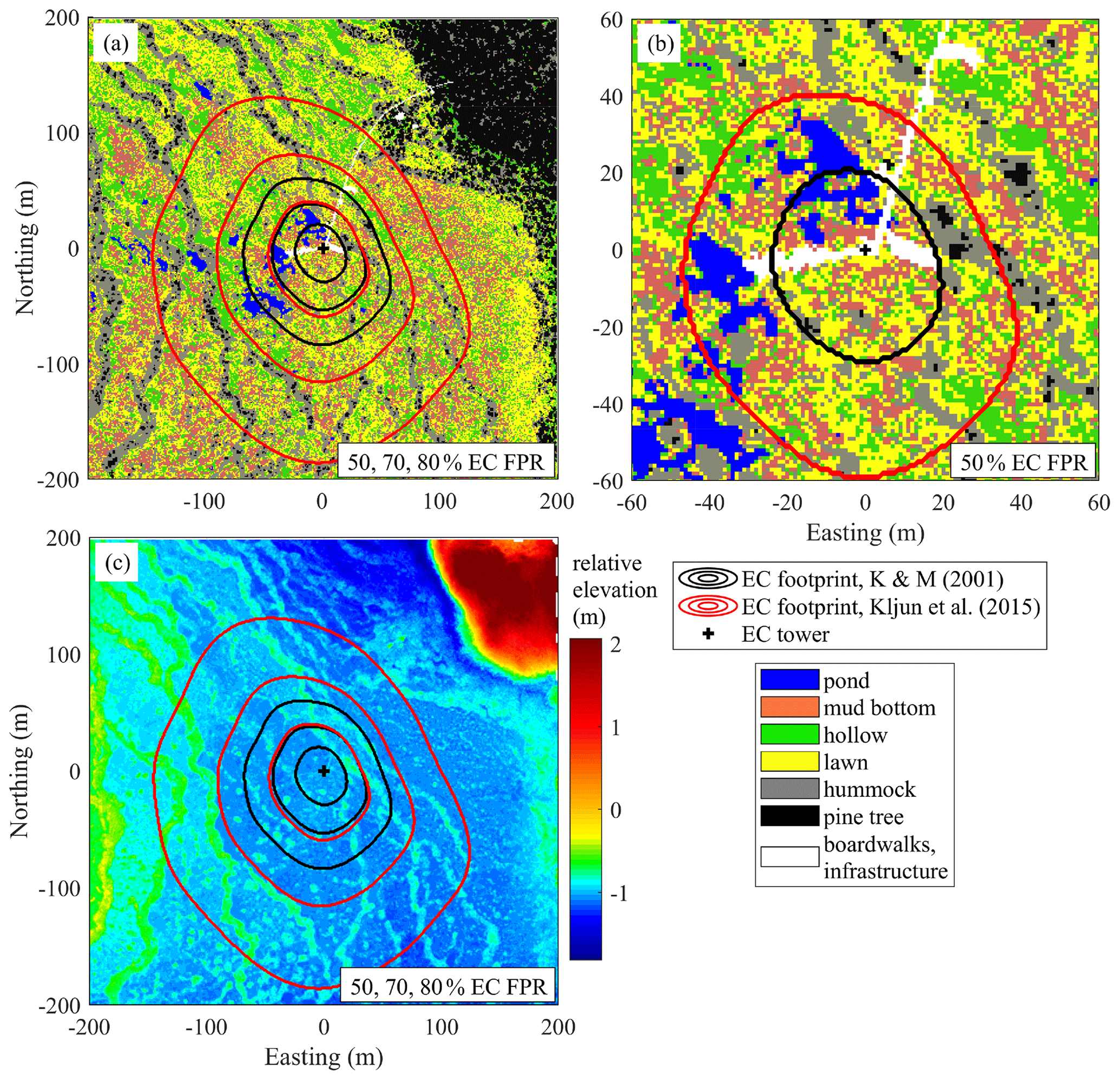
Figure 2Site characteristics obtained from the helicopter survey in May 2013. (a) Surface cover map at 1 m resolution showing a 400 × 400 m patch of landscape centered on the EC tower. The cumulative Kormann and Meixner (2001) and Kljun et al. (2015) flux footprints are given by 50, 70 and 80 % contribution contours. (b) Close-up map, focusing on the 50 % cumulative footprint zones. (c) Digital elevation model derived from a lidar scan. Note that the 70 % Kljun et al. (2015) isoline coincides with the 50 % Kormann and Meixner (2001) isoline. FPR – footprint.
Annual campaigns for leaf area index (LAI) measurement were undertaken at the site in 2012–2015. The representative microforms were covered by three replicate plots 60 cm × 60 cm in size, 18 in total. Within each plot, five small subplots were defined for the manual measurement of leaf number. This measurement was made approximately twice a month throughout the growing season, and simultaneously, average leaf size of each species was defined with a scanner. To obtain the leaf area of the subplots, the leaf number was multiplied by the average leaf area. These community-specific LAI values were then averaged and weighted by their area fractions within the EC footprint to yield the ecosystem-scale value (Korrensalo et al., 2017). The years of 2011 and 2016, when LAI was not measured, were filled with the 2012–2015 average LAI, as no LAI anomalies were visually detected in either 2011 or 2016 (Aino Korrensalo, personal communication, 2021).
2.2.3 Aerial imaging
An airborne survey combining lidar scanning and aerial photography was conducted by helicopter in May 2013 (Korpela et al., 2020). The data at the original resolution of 4 cm per pixel were processed and converted into a surface cover map and a digital elevation map (Fig. 2). As the individual microforms measure roughly 1–2 m2 in area, and in order to mitigate the motion blur present in the images, the resolution of all maps was coarsened to 1 m2 per pixel.
Table 2Proportions of the surface types and microforms, expressed as area percentage (first column) or weighted by the cumulative footprints, Kormann and Meixner (2001) and Kljun et al. (2015) (second and third columns).
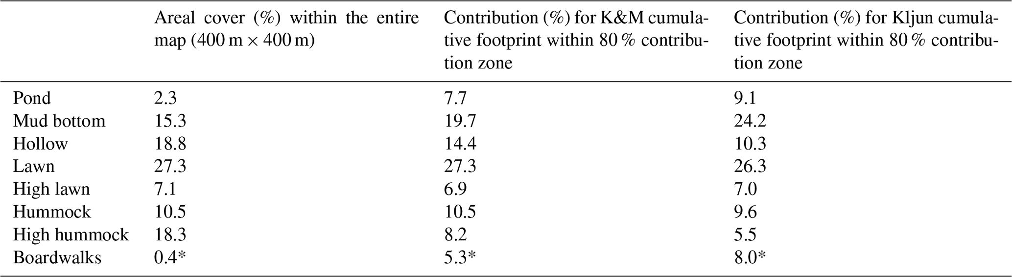
* Overestimate.
The proportion of each microform for the whole extent of the map (400 m × 400 m, centered on the EC tower) and its proportions weighted by the two footprint models were roughly similar (Table 2). Note that due to the proximity of the EC tower to the ponds (as was intended on the site planning stage) and boardwalks, their share in the EC flux source is comparatively higher than the 400 m × 400 m map means. The boardwalks extending in the western and eastern directions from the EC tower raft were built in April–June 2012, after the first measurement season. These building works caused only insignificant ecosystem damage, as no changes in the peat surface and vegetation cover around the new boardwalks were apparent. Also note that when the boardwalks some 30–40 cm wide are rescaled to the resolution of 1 m, their area becomes somewhat exaggerated.
2.3 EC flux footprint modeling
EC scalar flux footprints were calculated using the popular Kormann and Meixner (2001) and Kljun et al. (2015) models. The footprint lengths are very dependent on roughness length z0, necessitating its careful calculation and quality control. The 30 min average values of z0 were calculated using the expression
where z is the height above ground, κ the von Kármán constant, U the wind speed at level z, u∗ the friction velocity at level z, and the stability correction function defined, following Beljaars and Holtstag (1991), as
with , a=0.7, b=0.75, c=5 and d=0.35. The 30 min z0 values were used to model the footprint for each 30 min period so as to account for the variation in z0 due to the temporal changes in stability (Zilitinkevich et al., 2008) and directional variation in surface roughness. It was necessary to filter the calculated 30 min z0 values for very stable nocturnal conditions, which initiate a decoupling phenomenon. At nighttime thermal decoupling, which in Siikaneva typically happens below the EC measurement height (unpublished data), spikes in are observed which can be interpreted as airflow losing contact with the surface; therefore, the z0 values at > 12 and/or u∗ < 0.1 m s−1 were eliminated. High 30 min average z0 values may also occur at strongly convective conditions, when high instability is combined with low wind speeds, but those values are retained, with only the extreme values z0 > 3 m being excluded. The z0 values remaining after such filtering were from 0 to 3 m, with 80 % of the values being between 0 and 0.1 m and the most probable value being 0.03 m. The displacement height was set to zero as the surface roughness elements are small and sparse.
Footprint estimates were calculated on a 1 m × 1 m grid in order to match the resolution of the surface cover map. The footprint nodes lying further than 200 m away from the origin (coinciding with the location of the EC tower) were excluded from analyses. Such an exclusion of the map corners was necessary since, should they have been preserved, there would have been a bias between the footprints extending towards the corners and those extending in N, E, S and W directions due to the difference in the number of nodes. Finally, since a fraction of the EC signal (roughly 10 %–20 %) comes from beyond a 200 m distance from the tower, all footprint values within this domain were normalized by their cumulative sums in order to set them to unity.
2.4 Modeling the CO2, CH4 fluxes and EC flux gap-filling
The EC fluxes were modeled and gap-filled using the method similar to that in Alekseychik et al. (2017). In the initial modeling trials, Re, and GPP showed clear responses to peat temperature and PAR but much more complex relationships with WTD, making it impossible to capture the combined effect of environmental drivers on fluxes by fitting a single function to all data. As the dataset includes both long (> 15 d, mainly on the edges of the growing season) and short (< = 15 d) gaps, a special modeling approach was needed to fill the long gaps with robust, defensible estimates of GHG exchange and closely imitate the fluxes during shorter gaps. For gap distribution, see Fig. 5.
Table 3Parameters of the fits for Re, GPP and made using all quality-controlled data. The 95 % confidence intervals are given in parentheses.
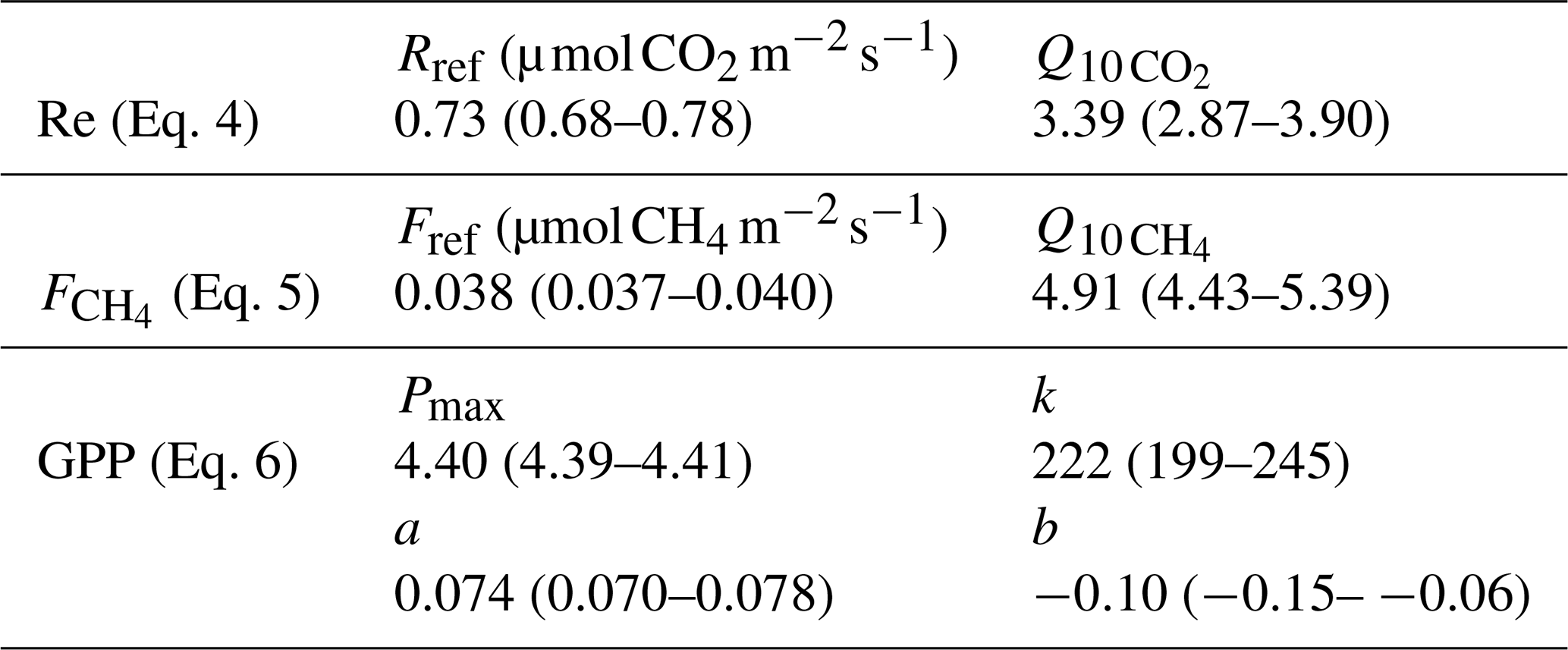
The models to fill the long gaps were obtained by fitting the standard Q10 and Michaelis–Menten-type expressions to all available quality-controlled Re, GPP and data,
where Reref and Fref are the reference ecosystem respiration and CH4 flux (model value at 12 ∘C), Pmax the maximum photosynthesis, k the value of PAR at GPP = 0.5 Pmax, PAR the photosynthetically active radiation, and and the temperature sensitivity parameters for respiration and CH4 flux, respectively. The resulting model parameter values are summarized in Table 3. The Michaelis–Menten expression for GPP is expanded with a peat temperature module as it was found to improve the fit, adding the linear function parameters a and b. Tp20 was chosen as the driver of as it performed slightly better (about 5 %) than Tp5 in terms of model R2, RMSE and error sum of squares (SSE). A reference temperature of 12 ∘C was used for both Re and (Eqs. 4 and 6) as a representative peat temperature at the site.
To fill the short (< 15 d) gaps, another set of models was constructed using the sliding time window approach. This approach allows for closely imitating the weather-dependent changes in fluxes without a detailed prior knowledge of the drivers. For Re and , Eqs. 4–5 were once again used; that for GPP, however, was simplified by eliminating the temperature module, as the information on the temperature variations would be implicit in the time-resolved model parameters:
The sliding time-window models were recalculated with a daily step, using the data from a period of 15 d for Re, 10 d for GPP and 5 d for . The resulting daily values of Reref, Fref, Pmax and k were linearly interpolated to each 30 min period. Section 3.3 and Fig. 6 provide the calculated parameter time series. The time-resolved model parameters are a valuable by-product of this approach, as their variations on weekly to seasonal timescales can provide clues on flux controls, similar to normalized fluxes used in some other studies. Finally, Re, GPP and are gap-filled using a combination of the two above models: sliding time window model for short gaps, and general-fit models for long gaps. The sliding window model performed well. The R2 of the median daily model vs. measured fluxes was 0.71 for and 0.67 for NEE, which is similar to what Raivonen et al. (2017) obtained using a process-based model HIMMELI with the data from the nearby Siikaneva-1 fen. However, the model in this study seems to capture the mean level of fluxes better than Raivonen et al. (2017), with the mean ratio of the model–measured flux being 0.99 for , 0.99 for GPP and 1.02 for Re. Thus, the above model is fully adequate for the purposes of this study – gap-filling and imitating the mean daily to seasonal course of surface GHG exchange.
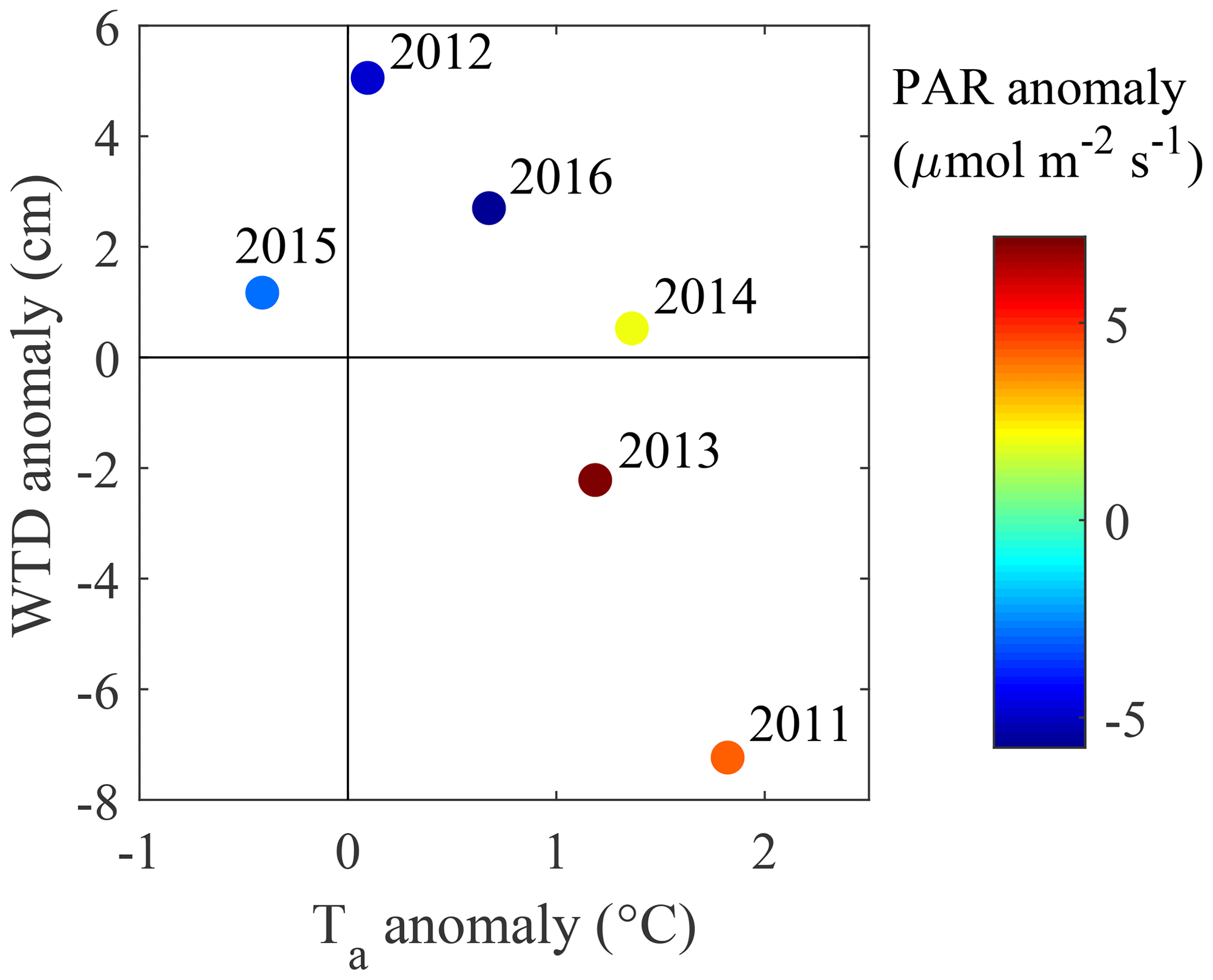
Figure 3June–August deviations in water table depth, air temperature and PAR, calculated as difference from the 6-year averages for WTD and PAR and 30-year averages for Ta.

Figure 4Time series of potential drivers of NEE, GPP, Re and . LAI is normalized by the annual peak value. The color lines in (a–d and f) represent weekly means, whereas in (e, h) they give daily average WTD and in (g) monthly precipitation sums. The black lines in (a–f) show the mean annual course of all years; the black markers in (g) are the monthly average precipitation of all years.
Table 4Average annual and summer air temperature, precipitation and water table depth in comparison with 30-year averages.

a 1981–2010, Pirinen et al. (2012). b The average of 2011–2016, as no longer-term data exist.
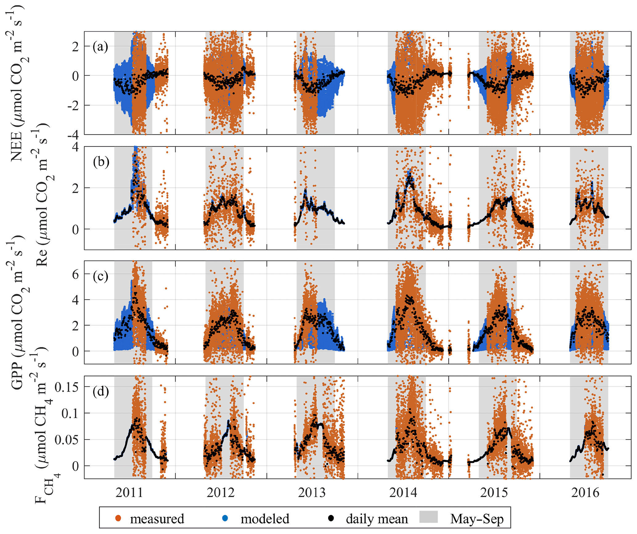
Figure 5Time series of measured and modeled 30 min values of NEE, Re, GPP and . The gray shading highlights the growing season (May–September). The model CH4 flux 30 min values are mostly hidden under the daily mean markers.
3.1 Environmental conditions
The climate is south boreal, with the mean 30-year average annual precipitation (liquid equivalent) being 711 mm and air temperature 3.5 ∘C (Table 4). The summer is typically warm and relatively dry, having a 30-year average air temperature of 14.6 ∘C and precipitation of 252 mm. The weather in 2011–2016 represented a range of conditions from warm–dry–sunny to cool–moist–cloudy (Fig. 3). Most of the years were warmer and drier than the 30-year average. Figure 4 shows the seasonal variation in the main environmental drivers. The year 2012 was atypical due to its low temperatures and ample precipitation, whereas another cool year 2015 had a sunny but dry autumn and an early drop in LAI (Fig. 4g and h). Normalized LAI was rather similar in the rest of the study years. The year 2011 had an untypically dry spring and summer, which resulted in the lowest instantaneous WTD of −25 cm and the lowest mean summertime WTD of −20 cm. The dry conditions of 2011 were also evident in the sharply increased diurnal amplitude of the peat temperature at 5 cm depth, implying the top peat layer and moss capitula may have been desiccated. The highest average growing season WTD of −7 cm was observed in 2012 (Fig. 4e).
3.2 Seasonal variability in the CO2 and CH4 fluxes
The EC flux time series shown in Fig. 5 reveal the typical seasonality with pronounced summer maxima. The measurements were mostly conducted during the growing season, with some autumn and winter periods covered in 2011–2012 and 2014–2015. Both the CO2 and CH4 fluxes are at their highest during the growing season from May to September. While the seasonal curve of NEE does not appear to show a marked deviation from the typical domed shape, its daily variation responded strongly to environmental conditions on a weekly to biweekly scale, with the beneficial conditions resulting in peak daily mean NEE of about −1…−1.5 and cool–cloudy–rainy weather reducing that to zero. The seasonality of the partitioned CO2 fluxes varied markedly between the years. The years 2011 and 2014 yielded higher seasonal peaks in GPP and Re than in the other years, corresponding with the periods of the warmest weather. Maximum GPP reached 4.3–4.5 in 2011 and 2014, which is substantially higher than 3.0–3.1 observed in the other years. Correspondingly, the maximum daily mean respiration reached 3.5 in 2011 and 2.7 in 2014, while the other years showed 1.6–1.9 at the peak. The summer peaks in CH4 flux in 2011 and 2014 closely matched those in GPP and Re and also resulted in the highest daily averages reaching 0.1 . In the other years, CH4 flux daily means reached 0.07–0.08 with an overall smoother seasonal maximum.
Table 5Contributions of the non-growing season fluxes to the total measured period.
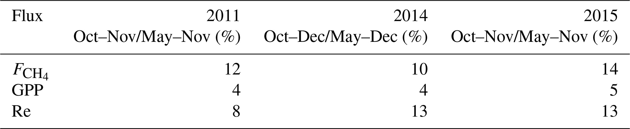
The importance of the non-growing season fluxes (October–Apr) was also analyzed. The spring peak of CH4 emission associated with the thaw period in April and May contributes only a minor, although non-negligible, fraction of the spring–summer total. In 2012, elevated net emission lasted for about 8 d (25 April–3 May) and in 2013 10 d (22 April–5 May). These periods supplied roughly 4 % of the cumulative CH4 emission of 25 April–31 August 2012 and 22 April–31 August 2013. Based on the partially covered winters of 2011–2012 and 2014–2015, the cumulative wintertime season fluxes were relatively small but non-negligible similar to the observations by Alm et al. (1999b). In 2011, the October–November contributions to May–November cumulative fluxes were as follows: 12 % for , 4 % for GPP and 8 % for Re. In 2015, the corresponding values were 14 %, 5 % and 13 %. Finally, in 2014, October–December contributed 10 % of , 4 % of GPP and 13 % of Re to the May–December totals (see a summary in Table 5).
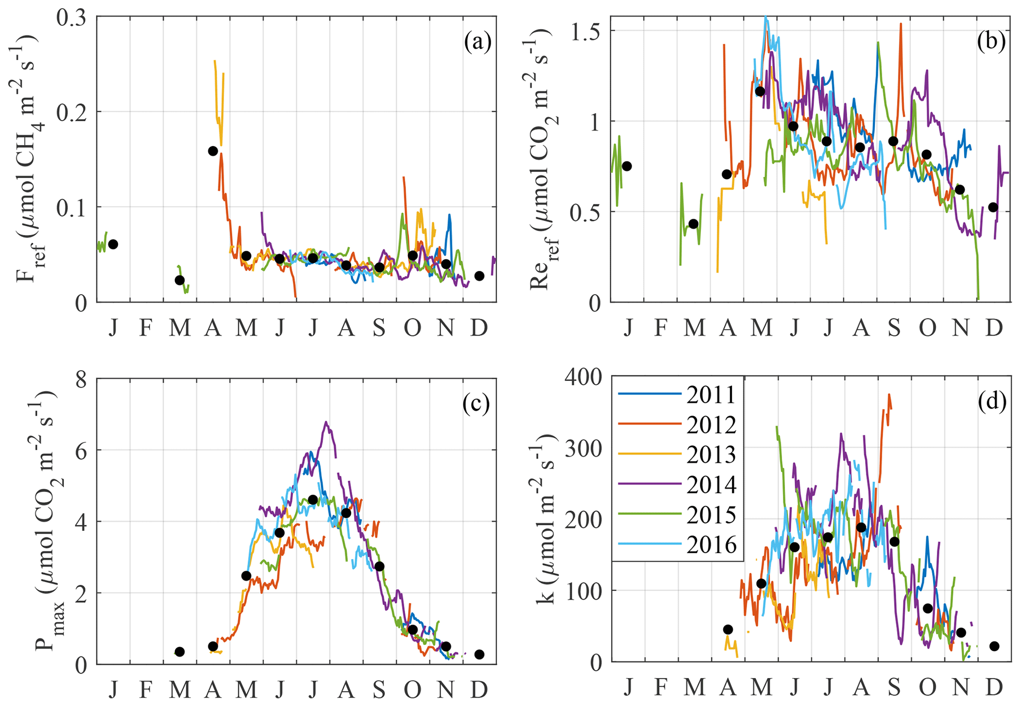
Figure 6Time series of CO2 and CH4 flux model parameters (Eqs. 4–6): (a) Reref, (b) Fref, (c) Pmax and (d) k. Monthly averages across years are shown with black dots.
3.3 Drivers of the seasonal variation in CO2 and CH4 fluxes
Figure 6 shows the temporal course of GPP, Re and model parameters (Eqs. 4, 5 and 7) and reveals their well-defined seasonalities and interannual differences. The CH4 reference flux has pronounced maxima in April and October–November (Fig. 6a), when the emissions may have been dominated by ebullition which is not controlled by temperature (so that high efflux coincided with low peat temperature). Between June and September, Fref falls on average from 0.045 to 0.035 . Reref (Fig. 6b) peaks in May at 1.2 , stagnates for the rest of the growing season and thereafter gradually drops to about 0.5 by December. However, this behavior is again detectable only on a monthly average basis. k and Pmax (Fig. 6c and d) have broad maxima in the middle of the growing season, more pronounced in Pmax than in k, in apparent relation with the LAI seasonality.
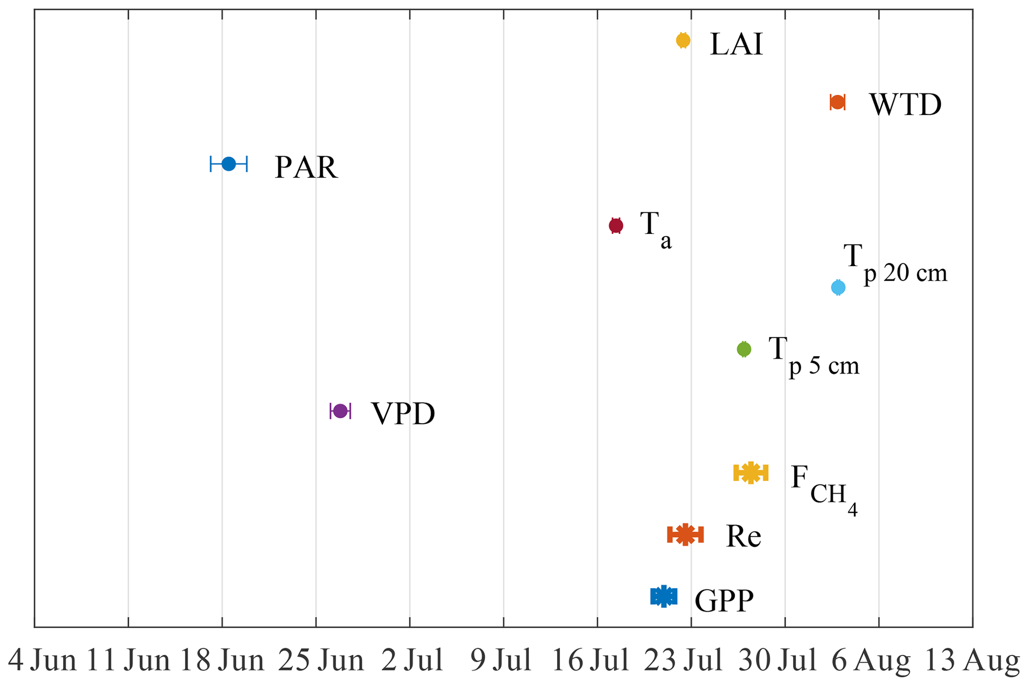
Figure 7The 6-year average timing of the annual peaks in fluxes and their potential drivers. The bars give the 95 % CI of the peak x value.
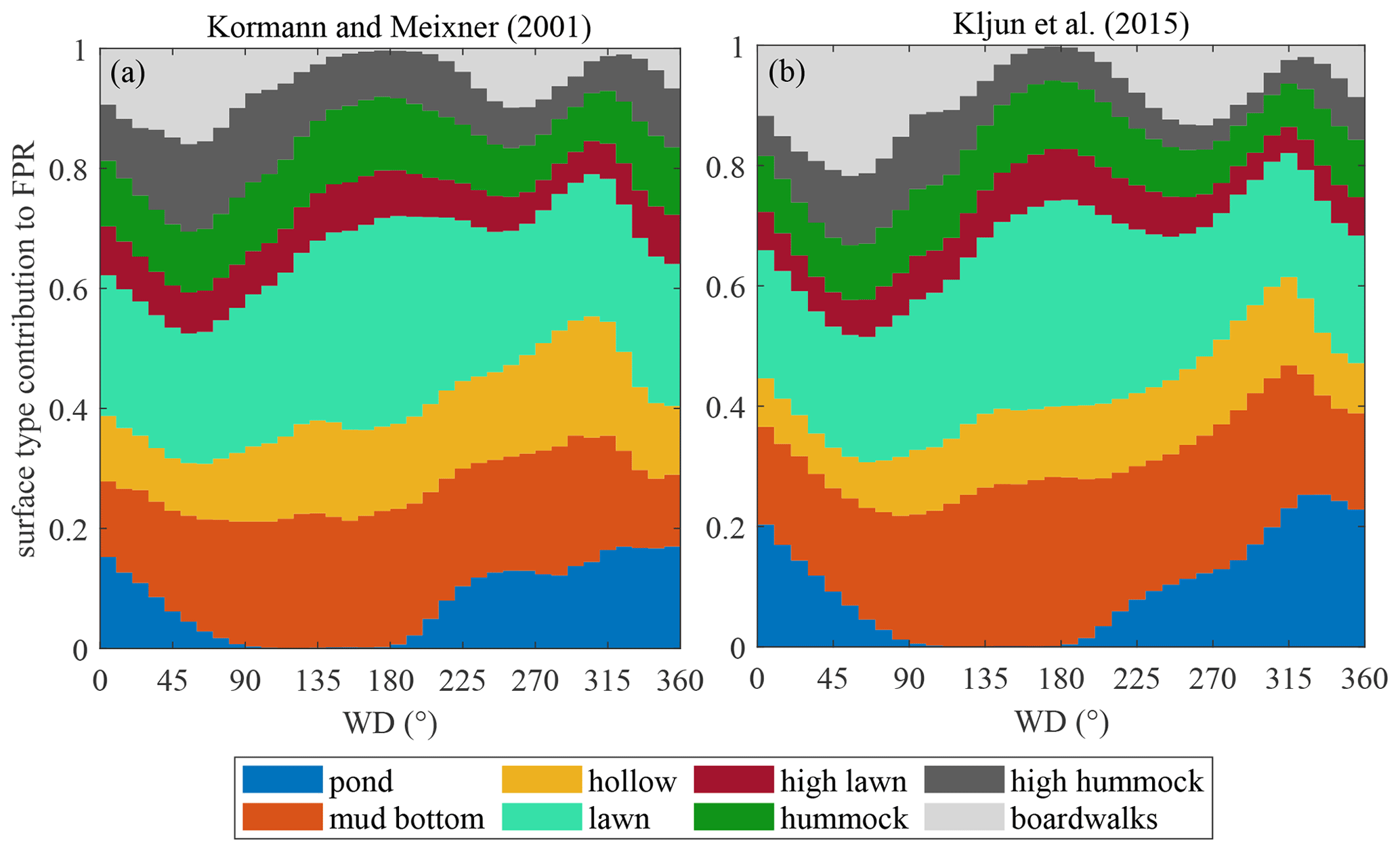
Figure 8Surface type contributions to surface exchange versus wind directions, presented as means over 10∘ Wind direction (WD) bins using all available data.
The timing of seasonal maxima in fluxes and environmental drivers were explored by fitting the Gaussian function to GPP, , Re and their physical drivers (log-linear function for LAInorm; Wilson et al., 2007), regressed against the day of year. The mean seasonal peak was estimated as the peak of the fit curves (Fig. 7). The peaks so derived mostly fall between the days 199 and 216, except those of vapor pressure deficit (VPD) and PAR that occur on days 171 and 178, respectively.
3.3.1 The effect of footprint variation
In heterogeneous mires, the variation in the EC footprint, controlled by wind direction and stability, may contribute to flux temporal variability, complicating the interpretation of EC fluxes (Tuovinen et al., 2019). Curiously, the two models, Kormann and Meixner (2000) and Kljun et al. (2015), produce quite similar surface compositions (Fig. 8) despite a significant difference in footprint length (Fig. 2). The variations in stability did introduce some variation in the footprint zone elongation, but did not cause significant changes in the footprint composition. The footprint composition, however, did vary with wind direction. The pond contribution ranges directionally from zero to about 20 %, being the most significant change, while the shares of the other microforms vary by about 10 %.

Figure 9Variation in June–August fluxes and flux model parameters with wind direction. (a) Variation in the CO2 and CH4 flux model parameters; (b) measured fluxes. The markers are bin averages normalized by the highest bin-average value for clarity.
The question of whether the directional variation in footprint composition has a noticeable effect on CO2 and CH4 fluxes is addressed in Fig. 9, which presents both the measured fluxes and the reference flux obtained by moving-window modeling (Eqs. 4, 5 and 7). The relative variation in reference fluxes was estimated as the difference between the highest and lowest bin averages (Fig. 9a) and proved to be broad, about 60 % in Reref, 40 % in Pmax and 20 % in Fref. The measured fluxes showed a similar directional variation (Fig. 9b). Importantly, in the western sector, roughly corresponding to the highest pond contribution, Pmax and Reref show a downward peak while the Fref shows an upward peak.
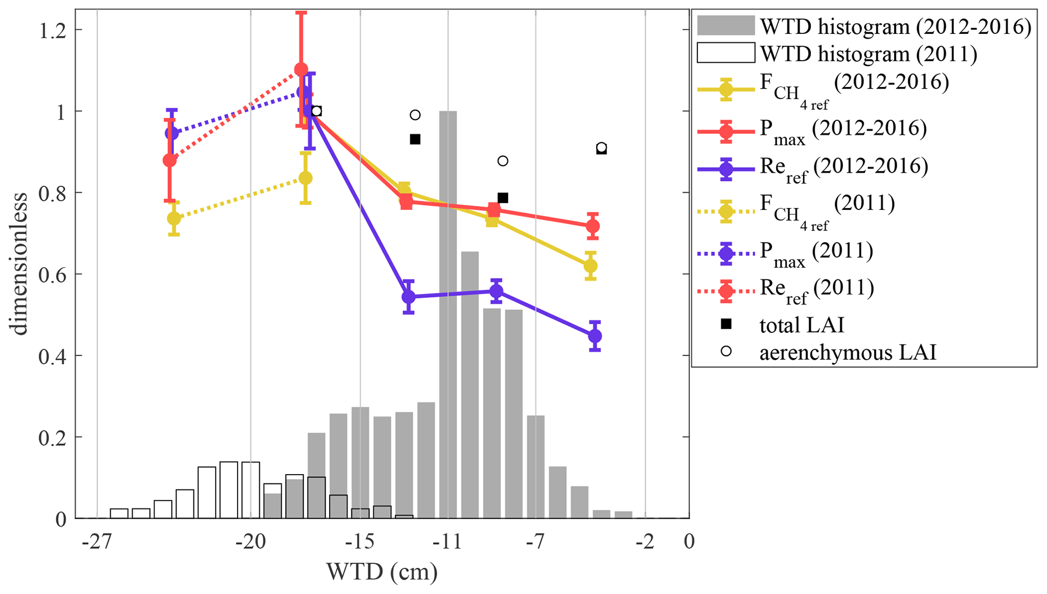
Figure 10Reference fluxes for and Re and maximum photosynthesis Pmax vs. water table depth, calculated as averages for the data within five WTD bins (marked by vertical lines), normalized by the value of the maximum bin average, along with the corresponding air temperature and measured LAI bin averages. The 2011 data are normalized by the 2012–2016 maxima, thus yielding values above unity. The data are from the period of June–August. The uncertainty bars give 50 % parameter CI. The WTD histogram is shown as gray bars. WTD histograms and flux parameters are shown separately for 2011 and 2012–2016.
3.3.2 Response to dry and hot conditions
Our dataset includes a markedly dry period of 2011. The response of the carbon fluxes to low-WTD conditions was evaluated by fitting Eqs. (4), (5) and (7) in five WTD bins (Fig. 10) in order to estimate the effect of dry conditions on flux model parameters. The data of 2011 are shown separately for better contrast with the higher-WTD conditions of the other years. When WTD is less than 15 cm, Pmax, Fref and Reref do not vary with water table. At a lower WTD (−20 > WTD > −15 cm), all of them are maximized. The two bins representing 2011 show that at yet lower WTD (< −20 cm), the reference fluxes stagnate or are slightly reduced. The parameter values in the −20…−15 cm bin, where the data of 2011 and 2012–2016 overlap, indicate similar Pmax and Reref but a lower Fref in 2011 compared with 2012–2016.
3.4 Drivers of the interannual variation in CO2 and CH4 fluxes
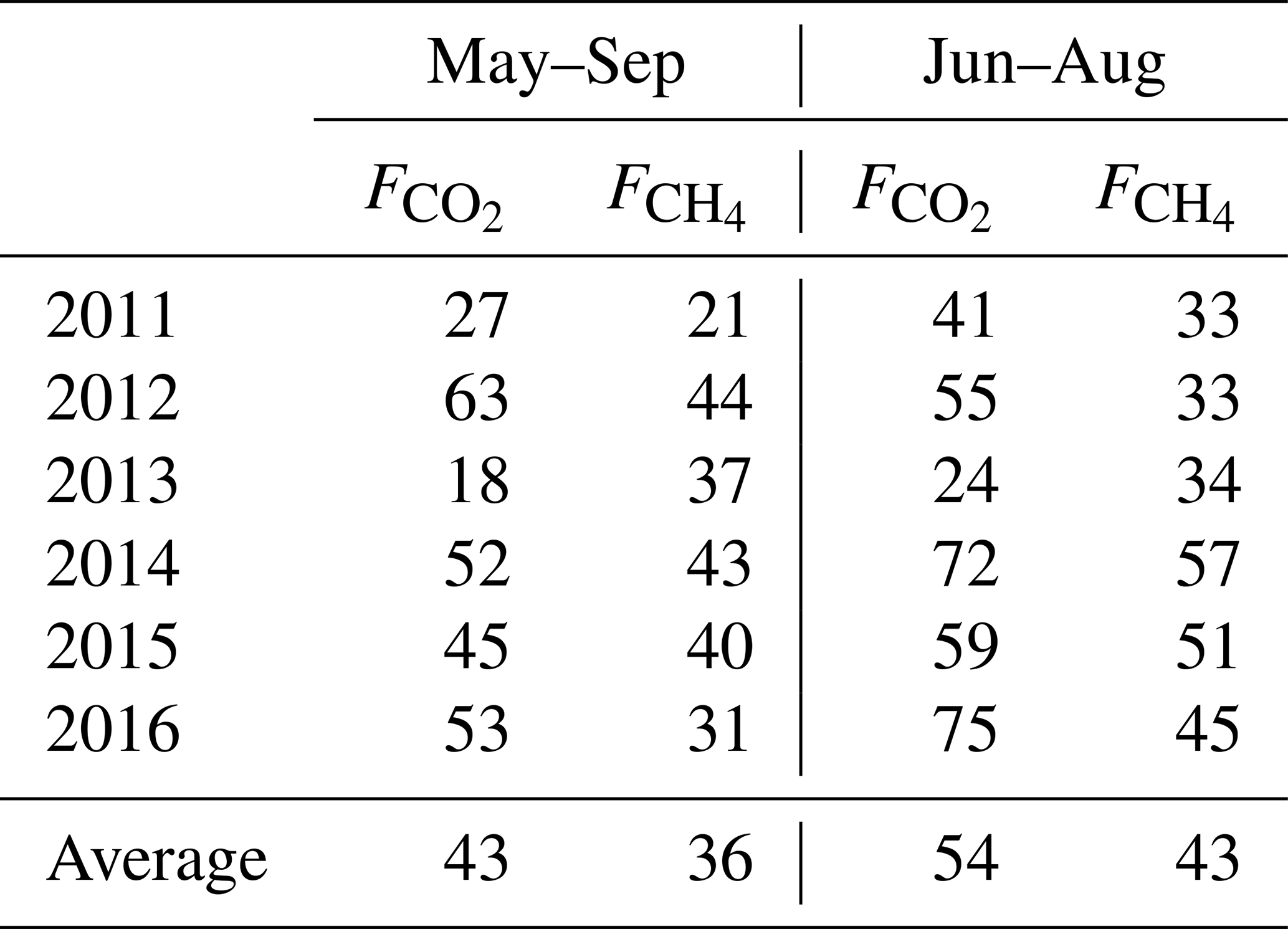
The cumulative growing season (May–September) NEE, its components and the net CH4 emission are summarized in Table 5. The typical summertime sums up to 4.8–6.4 g C m−2 and in the growing season 6.4–8.4 g C m−2. The summertime Re is 100–150 g C m−2 and GPP about 150–200 g C m−2, resulting in a May–September NEE of −20 to −64 g C m−2. May and September make a small addition to Re and GPP, raising the average cumulative NEE from −49 C m−2 in June–August to −61 g C m−2 in May–September.
Table 6Cumulative gap-filled summer and growing season CO2, CH4 fluxes and their 6-year averages, in g C m−2. The relative uncertainty is calculated using the May–September 6-year mean cumulative fluxes as 10 % for , 40 % for NEE, and 20 % for Re and GPP. In 2013, the NEE, Re and GPP uncertainties are assumed to be double due to poor CO2 EC flux data coverage. The last column gives the average cumulative fluxes with 2011 and 2013 excluded as the years with the lowest EC data coverage.
We attempted to estimate the uncertainty of cumulative fluxes by comparing the results of the current gap-filling method (Sect. 2.4) with those methods that were eventually discarded. The different gap-filling approaches led to a relative variation of some tens of g C m−2 in Re and GPP and about 0.5 g C m−2 in . In the year 2013 having the worst data coverage (Table 1), the cumulative GPP estimates by different gap-filling methods ranged between 190 and 270 g C m−2 (i.e. up to 20 % relative uncertainty on the average of 235 g C m−2), while in the rest of the years the range was much smaller (20–30 g C m−2 around the average GPP, or about 10 %). These relative uncertainties in GPP and Re, however, aggregate to a rather high relative uncertainty on May–September cumulative NEE, which may be estimated at 30 %–40 % of the 6-year mean May–September cumulative NEE. The relative uncertainty of cumulative NEE for 2013 alone is difficult to gauge; it may be much higher than in the other years so the net cumulative CO2 uptake is quite uncertain. However, it is a likely result and is treated as such in the following. Given these considerations, the seasonal cumulative values presented in Table 6 should be taken with caution as they contain a large proportion of gap-filled data. The uncertainties presented in Table 6 are close to the 25 g C m−2 year estimate of the error contributed by gap-filling by Moffat et al. (2007).
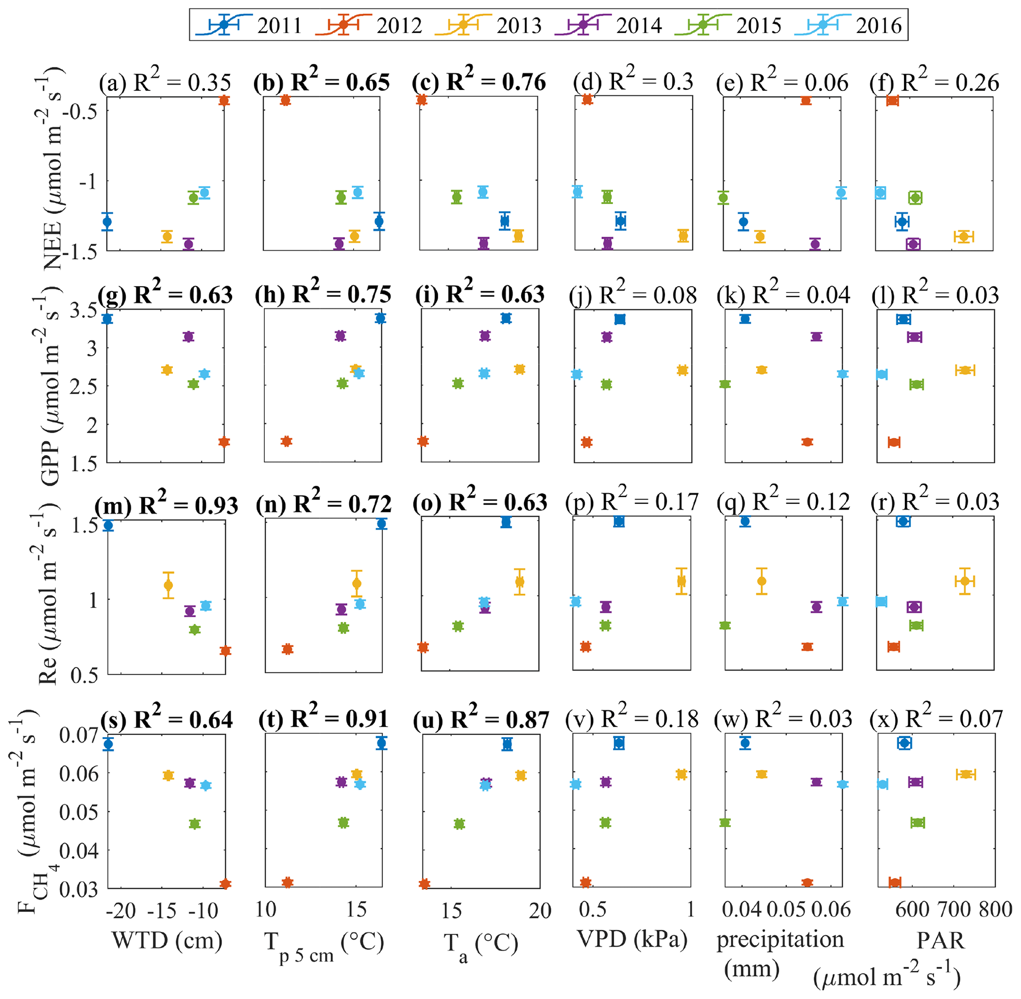
Figure 11May–September mean gap-filled fluxes versus averages (or cumulative, in the case of precipitation) of environmental drivers.
The year-to-year variability of the gap-filled fluxes strongly correlates with the variability of some environmental parameters (Fig. 11). This analysis uses only June–August as the period of best data coverage. High air and peat temperature favor high GPP, Re and . At the same time, high fluxes correspond to low WTD and high VPD. This suggests that the CO2 fluxes and methane emission are temperature-controlled, and the dry conditions associated with warm weather do not impose strict limitations. This is true as long as the WTD is within the tolerance limits, i.e. above about −20 cm as shown in Fig. 10 – but such dry periods did not last long enough to drastically affect the seasonal balances. In fact, the WTD limitations on fluxes are detectable in the opposite extremes – the hot and dry 2011 and the cool and moist 2012. In both years, the summer and growing season NEE was reduced when compared with the other years. Such links between WTD and fluxes are likely to exist on sub-monthly timescales, but the averaging required to reduce the random error inherent to the flux model parameters (as in Fig. 10) means that the result requires the data from prolonged periods of WTD drawdown. Therefore, the above reasoning applies mainly to the difference between the dry summer of 2011 and the other years.
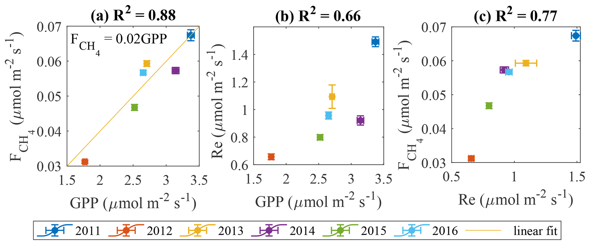
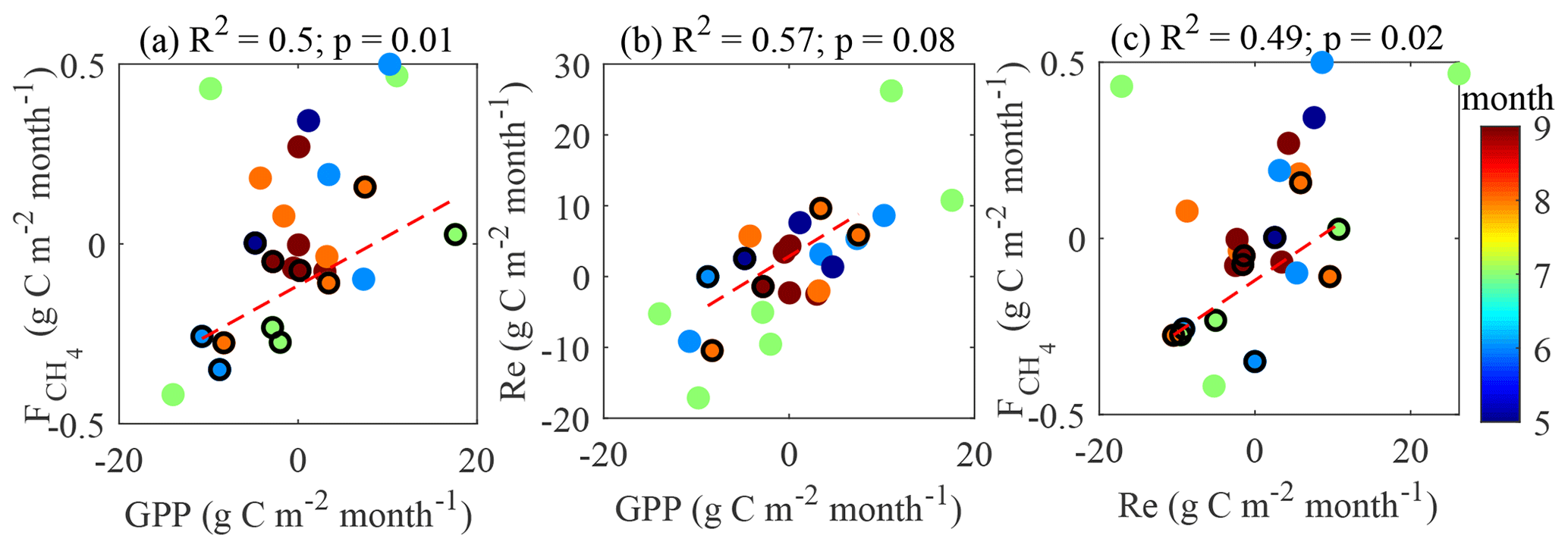
In line with the previous studies (e.g. Rinne et al., 2018), the cumulative GPP and values are found to be positively correlated (Fig. 12a). It is more difficult to identify the links in the other flux pairs (Fig. 12b–c). We acknowledge the big contribution of model flux to these gap-filled estimates, especially in 2013 (Table 1), which may have influenced the results in Figs. 11 and 12.
To support the above, the same relationships were tested by plotting monthly anomalies in the fluxes versus monthly anomalies in the drivers (Appendix B). The relationships between the monthly flux and control anomalies (for the months containing < 50 % model data) presented in Appendix B are similar to those in Figs. 11 and 12. This lends further support to the evidence of strong temperature control on the fluxes and the link between GPP and .
4.1 Filtering for low-turbulence conditions
The friction velocity threshold was evaluated from the relationship with EC CO2 and CH4 fluxes (Appendix A). As this method uses all available data, but only nighttime CO2 flux data, given equal random uncertainties one may hypothesize that using leads to a better-defined threshold. Here, the two thresholds matched – as they should have, owing to identical aerodynamic transport for scalars. However, the fact that the energy balance closure deficit continues into higher u∗ implies the presence of some other factors degrading the performance of EC technique, which might be related to poor representativeness of the footprint, or importance of storage fluxes. This observation calls for wider application of alternative strategies to EC flux filtering and a more critical approach to the standard u∗ filtering method.
4.2 Average growing season carbon exchange
The Siikaneva-2 bog was a net CO2 sink and CH4 source in each of the six growing seasons. The cumulative growing season (May–September) Re averaged 167 ± 33 g C m−2 and GPP 228 ± 46 g C m−2, yielding an NEE of −61 ± 24 g C m−2. These are within the range of the other bog studies reviewed above. For instance, middle taiga bog uptake measured near the Zotino station was between 40–60 g C m−2 between April and October in 3 years (Arneth et al., 2002). Cumulative May–August NEE of 66–107 g C m−2 was found by Humphreys et al. (2014) over 2 years in three Canadian bogs (Attawapiskat River, Kinoje Lake and Mer Bleu). Attawapiskat River and Kinoje Lake in the Hudson Bay lowlands are on par with Siikaneva-2, having May–August Re of about 160–170 g C m−2, GPP of 220–240 g C m−2 and NEE of 60–70 g C m−2. The shrub bog Mer Bleu produced an NEE of 88–107 g C m−2 with Re of 378–432 g C m−2 and GPP of 466–539 g C m−2.
The cumulative CH4 efflux in Siikaneva-2 averaged 7.2 g C m−2, which is slightly higher than the 3.6–4.6 g C m−2 reported by Vompersky et al. (2000) based on a growing season measurement campaign (184 d in May–October) on a south taiga ridge–hollow complex in European Russia. A much higher annual release of CH4 (19.5 g C m−2) was observed by Friborg et al. (2003) at the Plotnikovo site in the Bakchar bog (south taiga). A Canadian temperate shrub bog showed a 6-year average annual CH4 emission of 3.7 ± 0.5 g C m−2 (Roulet et al., 2007). Nadeau et al. (2013) report a cumulative summertime CH4 emission equivalent to 3.9 g C m−2 from a boreal bog in the James Bay lowlands in Canada.
The cumulative fluxes in Siikaneva-2 were close to those presented by Rinne et al. (2018) for the fen site Siikaneva-1 which is situated 1.3 km ESE of Siikaneva-2 (Fig. 1b). There, an NEE of similar magnitude was realized via Re and GPP approximately 200 g C m−2 higher than those in Siikaneva-2 (Rinne et al., 2018). At the same time, the methane emission is about 25 % lower in Siikaneva-2 bog than in Siikaneva-1 fen, estimated as the average ratio of the measured 30 min EC CH4 fluxes.
4.3 Drivers of interannual variability
The interannual differences in cumulative GPP, Re and CH4 emission were mainly controlled by temperature, with all fluxes increasing in warmer conditions, as suggested by both gap-filled growing season cumulative fluxes (Fig. 9) and monthly cumulative fluxes with the high model share months excluded (Fig. B1). In a year without positive or negative precipitation extremes, this leads to a rather stable May–September NEE of about −70 ± 24 g C m−2. In a year with ample precipitation, high WTD and low PAR (2012), this dropped to about −24 ± 24 g C m−2 (highly uncertain due to poor data coverage). In a year with a hot dry summer (2011), a moderately reduced May–September NEE of −47 ± 24 g C m−2 was observed.
The driest summer on record (2011) neither converted the peatland into a net CO2 source nor arrested the CH4 emission. This resilience seems to hold as long as the water table depth is above a threshold value, which is presumably at about −20 cm at this site (Fig. 9). Below that level, the reference fluxes cease increasing, implying that the positive effects of higher peat temperature have become balanced by the negative effect of dryness. However, the dry period of 2011 seems to have caused only a small decline in NEE, even though the WTD resided about 10 cm lower than the seasonal average for several weeks in a row. As warm summers clearly create conditions for high GPP, the reduction of NEE during drought is maybe more due to enhancement of respiration rather than suppression of photosynthesis. Strong enough drought can cause annual net CO2 emission from bogs, however. Alm et al. (1999a) report net release of carbon in a dry year at an open Sphagnum bog in eastern Finland, where NEE amounted to +80 g C m−2 (GPP = 205 g C m−2, Re = 285 g C m−2), with most of the loss occurring on hummocks, while lawns remained nearly C-neutral. In a Swedish temperate bog, Lund et al. (2012) observed near-zero annual average NEE due to drought in two out of four measurement years. A temperate bog became a considerable net source of CO2 (Arneth et al., 2002). An apparently saturating behavior of as a function of Re (Fig. 12c) is another indication of GHG emission rebalancing in dry conditions: as Re is enhanced, stagnates. Our results reinforce the view that only a strong drought is able to nullify net growing season CO2 sink and strongly reduce CH4 emission of a boreal bog. The drought timing may be important as well – hypothetically, an early spring drought may hamper the development of deciduous (shrub, graminoid) plant biomass, and so limit photosynthesis and CH4 emission for the rest of the summer; conversely, a drought initiated after the plant biomass has developed would have a lesser effect since the leaf area and the roots are already present and the vegetation has acquired a degree of resilience. This dynamic could have been in action at the Fäjemyr temperate bog, where a long and early drought lowered both GPP and Re, while a drought that started later in another year only increased Re (Lund et al., 2012)
A different set of limitations in 2012, now probably through low temperature and PAR, caused a stronger reduction in net CO2 sink than in 2011. The cumulative NEE went down by about 50 g C m−2, or about 70 % of the 2013–2016 mean NEE. A net annual emission of at 6.5 ± 0.7 g C m−2 was at the low end of the range for this site, although nearly identical to the emission in 2015 and 2016. This observation suggests that lowered air temperature and overcast conditions are a stronger limiting factor to plant growth and CH4 emission than moderately hot and dry conditions. Drops in solar radiation during daytime overcast–rainy weather limit photosynthesis (Nijp et al., 2015). It is difficult to tell whether the elevated WTD imposed a direct limitation on GHG production or transport. Previous studies show wet conditions without reduction in temperature result in high bog CO2 uptake. Friborg et al., 2003 estimated net CO2 uptake of −108 in Bakchar bog, south taiga. May–August NEE of −202 g C m−2 was observed in a wet year with a warm spring in the Mukhrino bog in Siberian middle taiga by Alekseychik et al., 2017; dry weather in the following year resulted in significantly lower net uptake due to higher Re and lower GPP at their west Siberian site (Alekseychik et al., unpublished data). European south taiga bog Fyodorovskoye had a similar weather sensitivity, being a sink of 60 g C m−2 in a wet year compared with a source of 25 g C m−2 in a dry year (Arneth et al., 2002). As a side note, carbon leaching may have been higher as ample precipitation must have boosted runoff and may have thus removed DOC that may have otherwise contributed to heterotrophic respiration and CH4 emission; Roulet et al. (2007) estimated an annual average net carbon leaching of 14.9 ± 3.1 g m−2, roughly one-third of the NEE observed in our study.
If the plants are expected to drive CH4 emission, LAI and should be well correlated on a seasonal scale with closely matching peaks. This, in fact, is partly confirmed by the analysis of seasonal peaks timing (Fig. 7). While LAI and GPP are in phase (Fig. 7), the magnitudes of their peaks in the individual years were not correlated (not shown), meaning that LAI might contribute to the seasonal shape of but does not determine its seasonal peak. Regarding the peak in , its occurrence between those in LAI and Tp20 is an independent indication that both controls might be important. The linear correlation between GPP and (Fig. 12a) comes as no surprise, as both become enhanced in warm conditions (Fig. 11), but it was not possible to check whether this reflects causality of just a similar reaction to environmental factors. With the present dataset, it was not possible to confirm the plant contribution to methanogenic substrate and CH4 transport. However, a pulse-labeling study of Dorodnikov et al. (2011) showed that recent photosynthates (on the timescale of a few hours to a few days) made a minuscule contribution to the total CH4 emission, whereas transport through Eriophorum vaginatum and Scheuchzeria palustris amounted to 30 %–50 % of the total methane efflux. Consequently, the apparent relationship between with net ecosystem productivity (NEP) might simply be due to the direct link between leaf area index (LAI) and NEP. Curiously, the slope of the GPP– linear relationship in Fig. 13a, 0.021 (CI 0.01–0.032) is significantly lower than 0.06 reported by Rinne et al. (2018) for the June–September period in a nearby fen, which might be related to the fact that sedges, the genus usually found to enhance CH4 emission, make up a larger fraction of GPP at the fen site.
4.4 Drivers of the seasonal CO2 and CH4 exchange
The carbon flux model parameters, resolved in time, display pronounced seasonal courses. The reference flux of respiration, Reref, peaks distinctly in May–June (Fig. 6a), which is clearly too late to indicate the release of CO2 stored during the snow-on period. There is a secondary Reref peak later in October. Fref is expectedly at the maximum in April–early May, at the time of snowmelt, whereas a weak correlation with LAI persists in the growing season (Fig. 6b). The autumn peaks in Fref are interesting, as they are not exactly correlated with those in Reref; transport through the sedge stems and peat freezing pushing out the bubbles are the potential mechanisms explaining the increased CH4 flux (e.g. Whiting and Chanton, 1992). Pmax has a well-defined bell-shaped seasonal course (Fig. 6c), with the peak coinciding with the maximum LAI, Ta and Tp and the lowest WTD (Fig. 7). The seasonality of k is similar to that of Pmax, albeit with more scatter.
It was difficult to explain the short-term (under 1 month) variation in the four model parameters. This may have largely resulted from random uncertainty and gaps in the EC flux data, but also partly due to the change in footprint and domination of plant species known to have different photosynthetic light response and phenology (Korrensalo et al., 2017). The strongest positive correlation is found between Pmax and Tp5, on a 2-week timescale; this should be seen in connection to the fact that the GPP model involving Tp5 (Eq. 6) showed the best performance.
Despite the rather incomplete EC data coverage, we attempted to evaluate the importance of the non-growing season fluxes. The period of October–April was captured in a few periods, as shown in Fig. 5. The magnitude of the spring peak was quite small, supplying about 4 % to the summertime CH4 emission in both years when it was measured. Rinne et al. (2018) found a similarly small spring peak that was absent in some years. The late autumn and winter fluxes, however, did contribute substantially (> 10 %) to the May–October or May–December Re and , but less so to GPP (< 5 %) (Table 5).
Variations in WTD seem to cause substantial variability in the flux model parameters (Fig. 10). Note the peak in CH4 and CO2 reference fluxes at WTD < −15 cm in both the dry 2011 and other years. The air temperature varies significantly across the bins, but LAI stays constant. As the positive effect of Ta on GPP is known, the Pmax maximization at the warmest temperatures is expected, as long as moisture is in good supply. In contrast, the Re and reference fluxes are independent of temperature by virtue of their formulation. This leaves us to hypothesize that it is the photosynthesis per leaf area, expressed here via its proxy, Pmax, which causes similar responses of Fref and Reref to WTD. The fact that all three parameters become saturated only at a rather low WTD hints at why a larger reduction in GPP, respiration and methane efflux is not observed in moderately dry and hot years. Lafleur et al. (2005) observed insensitivity of Re to WTD at the Mer Bleu shrub bog. At the same time, a lowered water table position is typically shown to be a negative effect on mire CH4 emission (e.g. Glagolev et al., 2001a, Kalyuzhny et al., 2009); however Rinne et al. (2018) propose the existence of an optimum WTD range (approx. −30…0 cm) maximizing the CH4 efflux in the fen Siikaneva-1 (SI1) close to the bog Siikaneva-2.
4.5 EC footprint variation effect
The actual EC source area is uncertain, as footprint models of Kormann and Meixner (2001) and Kljun et al. (2015) provided contrasting results regarding the footprint length (Fig. 2). Nonetheless, the EC data can be considered representative of the bog ecosystem, given the similarity between the cumulative footprint-weighted surface contributions and their abundance within the wider area (Table 2). The footprints had significantly different lengths, with the Kljun et al. (2015) model yielding shorter footprints. This is fully consistent with the results of Arriga et al. (2017), who observed the same relationship and found that the true source is between the estimates of the two models. Nevertheless, the variability in surface types between wind sectors is apparently more important than the variation with distance from the EC tower, because the surface type contributions calculated using the two models are very similar (Table 2). In a heterogeneous site such as Siikaneva bog, the directional variation in the microform contributions to EC flux does not come as a surprise (Fig. 8). The amplitude of variation in the lawn, mud bottom and pond contributions reaches 10 %–20 %; curiously, the KandM and Kljun models agree on this, despite differing on footprint length. Maybe of greatest interest are the directional differences in the pond contribution, with the maximum in 230∘–N–30∘ and minimum at 50–200∘. In a similarly heterogeneous tundra site, Tuovinen et al. (2019) found that the variation in the EC footprint with stability and wind direction induced a significant bias between the EC flux and the “true” upscaled flux of the region. Nevertheless, the cumulative contributions of the different microforms to the EC flux were close to their fractions over the 400 m × 400 m area centered at the EC tower, implying that the EC data are representative of the ecosystem-average fluxes.
The question is now as follows: is the effect of the ponds on the EC fluxes discernible, even despite their contribution varying with wind direction from 0 % to a maximum of 20 % depending on wind direction? In case the microforms have widely different C exchange rates, the footprint variation effect should, in principle, be discernible. Earlier chamber studies suggest that CH4 efflux from microtopography elements with lower elevation (hollows) is higher than that from ridges and hummocks (e.g. Glagolev and Suvorov, 2007; Glagolev and Shnyrev, 2008; Maksuytov et al., 2010). Alm et al. (1999a) observed annual CH4 fluxes ranging from 2 g C m−2 on hummocks to 14 g C m−2 on hollows. High CH4 emission was detected on ponds (Repo et al., 2007; Maksuytov et al., 2010) and float mats (Kazantsev et al. 2010). However, chamber studies in Siikaneva-2 bog did not find significant differences in CH4 efflux on different microforms (Korrensalo et al. 2017). Nevertheless, the EC data do show that both the normalized and the CH4 reference flux were actually elevated within the sector with the maximum pond contribution (Fig. 9). This apparent emission peak occupies only a part of the sector containing the ponds, meaning that either the individual ponds emit different amounts of CH4 or the anomaly is not related to ponds at all. The existence of the CH4 emission hotspot is independently confirmed by comparison of the chamber fluxes across the chamber plots located to the west, east and north of the EC tower; the western sector CH4 chamber flux is the highest (Aino Korrensalo, personal communication, 2019). The effect of ebullition may be ruled out based on the results of Männistö et al. (2019), who studied the variation in ebullitive CH4 flux from vegetation-free surfaces (ponds, pond edges, mud bottoms) and estimated that the relative growing season contribution of the ebullition on these surfaces to the integrated EC-scale flux amounts to 3 %–5 %. Boardwalks and other station infrastructure are concentrated in the W and NE sectors (Fig. 8) and appear to correlate with the CH4 peak in the W sector (Fig. 9). However, the boardwalk share is an overestimate due to rescaling the original aerial images to the map at the resolution of 1 m × 1 m. Second, the disturbance of peat due to the presence of boardwalks or chamber collars was presumably minor, as the CH4 emission hotspot had been present in 2011, before any infrastructure was built in the western sector, and no major traces of disturbance were seen on the mire surface. The drop in GPP and Pmax in the same sector is logical: less area covered by plants in the “pond” sector would lead to lower photosynthesis. This supports the idea of the potential pond origin of the detected CH4 emission peak. Re and Reref were significantly higher in the sector 0–130∘ than in 150–300∘, possibly due to the higher contribution of hummocks and lower WTD in the NE sector (Fig. 9; see also Korrensalo et al., 2017).
The average growing season CO2 and CH4 cumulative fluxes in the southern Finnish bog Siikaneva-2 are within the range of the previous estimates for other boreal bogs. The 6-year average May–September NEE is −61 ± 24 g C m−2, which splits into 167 ± 33 g C m−2 of Re and 228 ± 46 g C m−2 of GPP, whereas the cumulative net CH4 efflux is 7.2 ± 0.7 g C m−2. The variations in cumulative May–September Re, GPP and were positively correlated with the average air and peat temperatures, while water table level was not a limiting factor except in the driest of periods, which were too short to affect the seasonal balances. However, it proved difficult to separate the effects of the flux drivers due to their strong mutual dependency. The growing season cumulative GPP was well correlated with , as in the nearby fen (Rinne et al., 2018). The non-growing season fluxes were not negligible and need to be reassessed in future studies. However, this mostly relates to autumn and early winter, as the early spring photosynthesis was low and the spring peak noticeable, but its contribution was minor on the annual timescale.
Even in such a strongly patterned site, the surface heterogeneity was insufficient to conclusively demonstrate any footprint-related variations in EC fluxes. The upwind GHG sources were well integrated by the EC method, and there was not enough directional difference in surface cover. As a result, the contributions of the different surfaces did not vary with wind direction by more than 10 %–20 %, which is too small considering the joint uncertainties in the footprint model, microform map and EC fluxes. The dependency of Pmax on the ratio of vegetated to non-vegetated surfaces in the footprint was the only signal of surface heterogeneity in agreement with the known EC footprint composition. EC CH4 flux peaked in the western sector, possibly due to the higher proportion of ponds and higher WTD in that sector, but no correlation with the surfaces contributing to the EC flux was found. The complications with the interpretation of the EC data encountered in this study stem from highly correlated changes of the environmental drivers and the flux footprint, on the timescales from week to season. These limitations apply to all eddy-covariance sites, which calls for a more critical approach to EC data interpretation and modeling, including combining EC and flux chambers, cross-validation of the EC footprint models, and the detailed analysis of the ecosystem surface composition.
Figure A1 shows the normalized CH4 and CO2 fluxes and the energy balance closure plotted against u∗. While the normalized GHG fluxes both saturate at u∗ = 0.1 m s−1, the energy balance closure does so only at u∗ above 0.15 m s−1. As this analysis aims to identify the variation in the turbulent heat fluxes LE and H with u∗, ground heat flux (G) is omitted from the surface energy balance equation. The addition of G would lead to an increase in the surface energy balance (SEB) closure (SEBC), especially at low u∗, which mainly occurs at night, which may conceal the u∗ threshold at which the SEBC starts to degrade due to the deficit in latent heat flux (LE) and sensible heat flux (H).
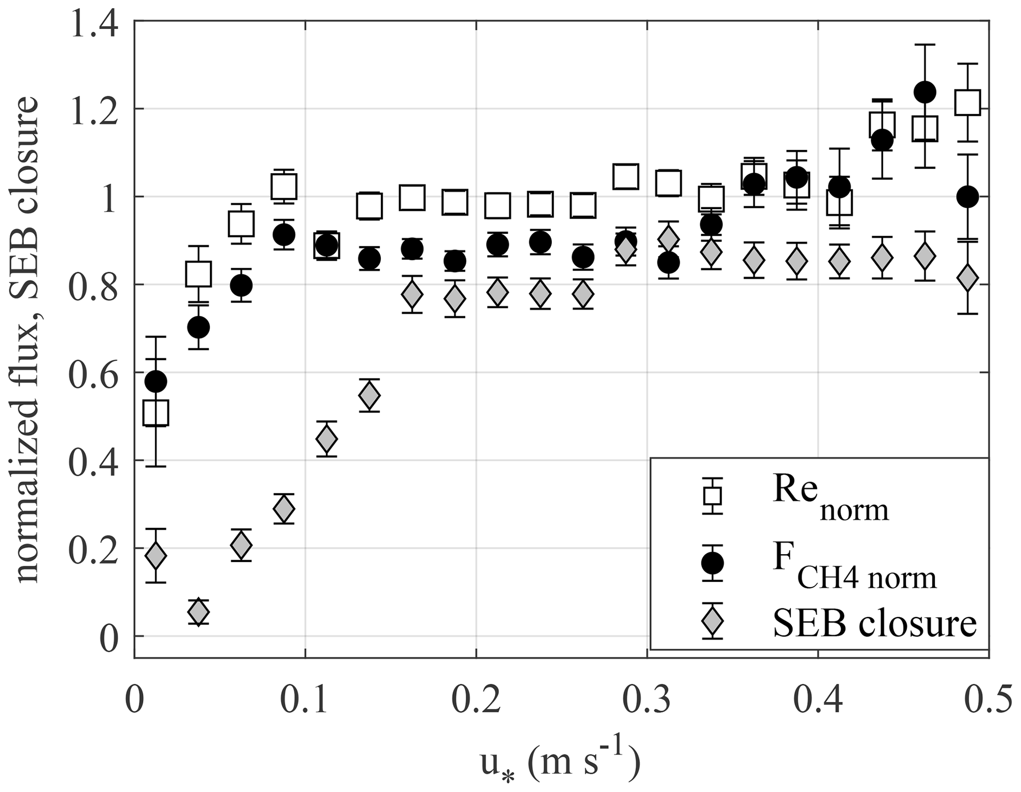
Figure A1Bin-median values of CO2 respiration (Re) and CH4 efflux, normalized by their temperature-based statistical models, and surface energy balance closure (SEBC = ) vs. friction velocity for May–October, with the bars giving SD of the median.
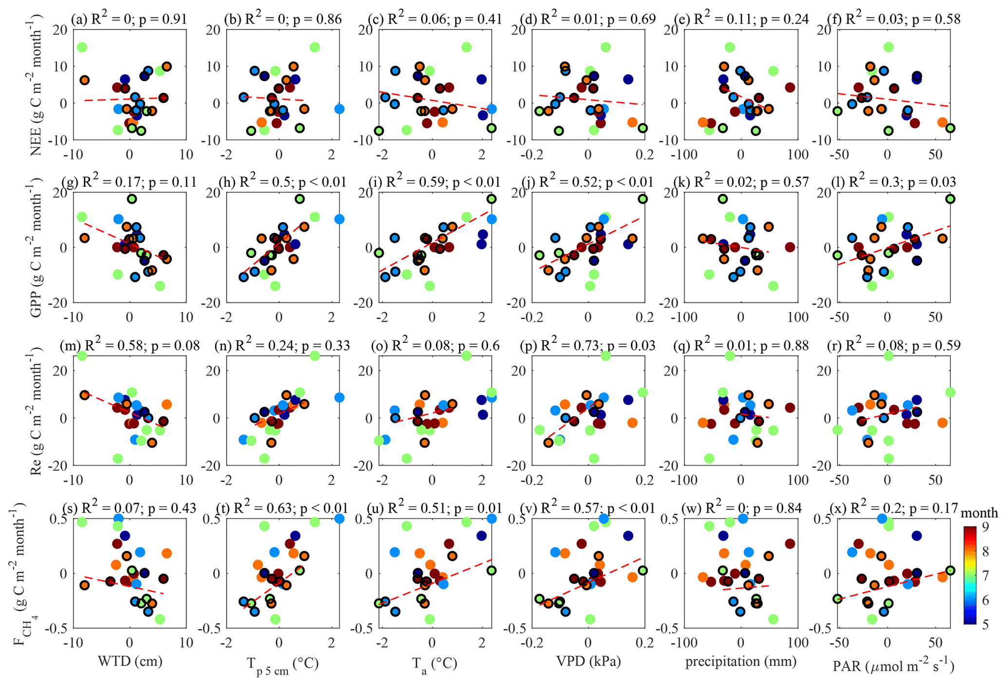
Figure B1Monthly anomalies in May–September fluxes plotted versus the monthly means of the environmental drivers. The months with > 50 % EC flux data coverage are shown with black circles and are used for linear fitting (red dash lines). Color coding shows the month number to ensure that the seasonal cycles do not influence the presented relationships.
The codes used in the preparation of this paper are available upon request from the authors.
Siikaneva-2 eddy-covariance and meteorological data can be downloaded from the FLUXNET repository, https://www.osti.gov/dataexplorer/biblio/dataset/1669639 (Vesala et al., 2020).
PA was partly responsible for the field measurements (eddy covariance, meteorology and soil), post-processed and analyzed the EC data, produced the figures, and wrote the paper text. AK conducted the vegetation sampling campaigns, analyzed the vegetation data and contributed to the text. IM helped to analyze the eddy-covariance data and contributed to the study design and the text. SL contributed to the text and provided extensive critical commentary. EST co-managed the Siikaneva-2 site, contributed to the text and provided critical commentary. IK processed the airborne imaging and remote sensing data and contributed to the text. TV helped formulate the aims and study design, co-managed the Siikaneva-2 site, and contributed to the text.
The authors declare that they have no conflict of interest.
Publisher's note: Copernicus Publications remains neutral with regard to jurisdictional claims in published maps and institutional affiliations.
Pavel Alekseychik and Samuli Launiainen acknowledge the support of the projects CLIMOSS (Climate impacts of boreal bryophytes – from functional traits to global models) funded by the Academy of Finland, decision no. 296116, 307192, 327180), and SOMPA (Novel soil management practices-key for sustainable bioeconomy and climate change mitigation, funded by the Strategic Research Council at the Academy of Finland, Decision no. 312912). Pavel Alekseychik is grateful for the Academy of Finland Flagship Programme for financial support to competence center Forest-Human-Machine Interplay – Building Resilience, Redefining Value Networks and Enabling Meaningful Experiences (UNITE) (decision 337655). Timo Vesala, Ivan Mammarella and Ilkka Korpela acknowledge Academy of Finland Flagship funding (grant no. 337549). Timo Vesala thanks the grant of the Tyumen region, Russia, government in accordance with the Program of the World-Class West Siberian Interregional Scientific and Educational Center (National Project “Nauka”).
This research has been supported by the Suomalainen Tiedeakatemia (grant nos. CLIMOSS project (decision no. 296116, 307192, 327180), the SOMPA project (decision no. 312912) and Flagship funding (grant no. 337549)).
Open-access funding was provided by the Helsinki University Library.
This paper was edited by Sebastian Naeher and reviewed by Joshua Ratcliffe and one anonymous referee.
Alekseychik, P., Mammarella, I., Karpov, D., Dengel, S., Terentieva, I., Sabrekov, A., Glagolev, M., and Lapshina, E.: Net ecosystem exchange and energy fluxes measured with the eddy covariance technique in a western Siberian bog, Atmos. Chem. Phys., 17, 9333–9345, https://doi.org/10.5194/acp-17-9333-2017, 2017.
Alm, J., Saarnio, S., Nykänen, H., Silvola, J., and Martikainen, P. J.: Winter CO2, CH4 and N2O fluxes on some boreal natural and drained peatlands, Biogeochemistry, 44, 163–186, 1999a.
Alm, J., Schulman, L., Nykänen, H., Martikainen, P. J., and Silvola, J.: Carbon balance of a boreal bog during a year with an exceptionally dry summer, Ecology, 80, 161–174, 1999b.
Arneth, A., Kurbatova, J., Kolle, O., Shibistova, O. B., Lloyd, J., Vygodskaya, N. N., and Schulze, E.-D.: Comparative ecosystem–atmosphere exchange of energy and mass in a European Russian and a central Siberian bog II. Interseasonal and interannual variability of CO2 fluxes, Tellus B, 54, 514–530, https://doi.org/10.3402/tellusb.v54i5.16684, 2002.
Arriga, N., Rannik, Ü, Aubinet, M., Carrara, A., Vesala, T., and Papale, D.: Experimental validation of footprint models for eddy covariance CO2 flux measurements above grassland by means ofnatural and artificial tracers, Agr. Forest Meteorol., 242, 75–84,2017.
Aubinet, M., Vesala, T., and Papale, D. (Eds.): Eddy covariance: a practical guide to measurement and data analysis, Springer Science & Business Media, Berlin, Germany, 2012.
Baldocchi, D. D.: ‘Breathing’ of the terrestrial biosphere: lessons learned from a global network of carbon dioxide flux measurement systems, Aust. J. Bot., 56, 1–26, 2008.
Beljaars, A. C. M. and Holtslag, A. A. M.: Flux parameterization over land surfaces for atmospheric models, J. Appl. Meteorol., 30, 327–341, https://doi.org/10.1175/1520-0450(1991)030<0327:FPOLSF>2.0.CO;2, 1991.
Bellisario, L. M., Bubier, J. L., Moore, T. R., and Chanton, J. P.: Controls of CH4emissions from a northern peatland, Global Biogeochem. Cy., 13, 81–91, 1999.
Bubier, J., Costello, A., Moore, T. R., Roulet, N. T., and Savage, K.: Microtopography and methane flux in boreal peatlands, northern Ontario, Canada, Can. J. Botany, 71, 1056–1063, 1993.
Bubier, J., Crill, P., Mosedale, A., Frolking, S., and Linder, E.: Peatland responsesto varying interannual moisture conditions as measured byautomatic CO2 chambers, Global Biogeochem. Cy., 17, 1066, https://doi.org/10.1029/2002GB001946, 2003.
Bubier, J., Moore, T., Savage, K., and Crill, P.: A com-parison of methane flux in a boreal landscape betweena dry and a wet year, Global Biogeochem. Cy., 19, https://doi.org/10.1029/2004gb002351, 2005.
Buttler. A., Robroek, B. J. M., Laggoun-Défarge, F., Jassey, V. E. J., Pochelon, C., Bernard, G., Delarue, F., Gogo, S., Mariotte, P., Mitchell, E. A. D., and Bragazza, L.: Experimental warming interacts with soil moisture to discriminate plant responses in an ombrotrophic peatland, J. Veg. Sci., 26, 964–974, https://doi.org/10.1111/jvs.12296, 2015.
Charman, D. J., Beilman, D. W., Blaauw, M., Booth, R. K., Brewer, S., Chambers, F. M., Christen, J. A., Gallego-Sala, A., Harrison, S. P., Hughes, P. D. M., Jackson, S. T., Korhola, A., Mauquoy, D., Mitchell, F. J. G., Prentice, I. C., van der Linden, M., De Vleeschouwer, F., Yu, Z. C., Alm, J., Bauer, I. E., Corish, Y. M. C., Garneau, M., Hohl, V., Huang, Y., Karofeld, E., Le Roux, G., Loisel, J., Moschen, R., Nichols, J. E., Nieminen, T. M., MacDonald, G. M., Phadtare, N. R., Rausch, N., Sillasoo, Ü., Swindles, G. T., Tuittila, E.-S., Ukonmaanaho, L., Väliranta, M., van Bellen, S., van Geel, B., Vitt, D. H., and Zhao, Y.: Climate-related changes in peatland carbon accumulation during the last millennium, Biogeosciences, 10, 929–944, https://doi.org/10.5194/bg-10-929-2013, 2013.
Davidson, E. A. and Janssens, I. A.: Temperature sensitivity of soil carbon decomposition and feedbacks to climate change, Nature, 440, 165–173, 2006.
Dorodnikov, M., Knorr, K.-H., Kuzyakov, Y., and Wilmking, M.: Plant-mediated CH4 transport and contribution of photosynthates to methanogenesis at a boreal mire: a 14C pulse-labeling study, Biogeosciences, 8, 2365–2375, https://doi.org/10.5194/bg-8-2365-2011, 2011.
Dunfield, P., Knowles, R., Dumont, R. T., and Moore, T. R.: Methane production and consumption in temperate and subarctic peat soils: response to temperature and pH, Soil Biol. Biochem., 25, 321–326, 1993.
Euskirchen, E. S., Edgar, C. W., Turetsky, M. R., Waldrop, M. P., and Harden, J. W.: Differential response of carbon fluxes to climate in three peatland ecosystems that vary in the presence and stability of permafrost, J. Geophys. Res.-Biogeo., 119, 1576–1595, 2014.
Fechner-Levy, E. J. and Hemond, H. F.: Trapped methane volume and potential effects on methane ebullition in a northern peatland, Limnol. Oceanogr., 41, 1375–1383, 1996.
Friborg, T., Soegaard, H., Christensen, T. R., Lloyd, C. R., and Panikov, N. S.: Siberian wetlands: Where a sink is a source, Geophys. Res. Lett., 30, 2129, https://doi.org/10.1029/2003GL017797, 2003.
Frolking, S. and Roulet, N. T.: Holocene radiative forcingimpact of northern peatland carbon accumulation and methane emissions, Glob. Change Biol., 13, 1079–1088, https://doi.org/10.1111/j.1365-2486.2007.01339.x, 2007.
Glagolev M., Inisheva L., Lebedev V., Naumov A., Dement'eva T., Golovatskaja E., Erohin V., Shnyrev N., and Nozhevnikova A.: The Emission of CO2 and CH4 in Geochemically Similar Oligotrophic Landscapes of West Siberia, in: Proceedings of the Ninth Symposium on the Joint Siberian Permafrost Studies between Japan and Russia in 2000, Sapporo, Japan, 23–24 January, 2001, Sapporo, Kohsoku Printing Center, 112–119, 2001.
Glagolev, M. V. and Shnyrev, N. A.: Methane emission from mires of Tomsk oblast in the summer and fall and the problem of spatial and temporal extrapolation of the obtained data, Moscow University Soil Science Bulletin, 63, 67–80, 2008.
Glagolev, M. V. and Suvorov, G. G.: Methane emission from wetland soils in middle taiga (by example of Khanty-Mansi autonomous district), Doklady po Ekologicheskomu Pochvovedeniyu, 2, 90–162, 2007 (in Russian with English summary).
Gorham, E.: Northern peatlands: role in the carbon cycle and probable responses to climatic warming, Ecol. Appl., 1, 182–195, 1991.
Humphreys, E. R., Charron C., Brown, M., and Jones, R.: Two bogs in the Canadian Hudson Bay Lowlands and a temperate bog reveal similar annual net ecosystem exchange of CO2, Arct. Antarct. Alp. Res., 46, 103–113, 2014.
Kaluyzhny, I. L., Lavrov, S. A., Reshetnikov, A. I., Paramonova, N. N., and Privalov, V. I.: Emission of methane at an oligotrophic peatland massif in northwestern Russia, Meteorol. Hydrol., 1, 53–67, 2009 (in Russian).
Kazantsev V. S., Glagolev M. V., Golubyatnikov L. L., and Maksyutov S. S.: Methane emissions from lakes in West Siberian wetlands, in: Proceedings of the EGU General Assembly 2010, Vienna, Austria, 2–7 May 2010, Geophysical Research Abstracts, 12, EGU2010-358, 2010.
King, G. M., Roslev, P., and Skovgaard, H.: Distribution and rate of methane oxidation in sediments of the Florida Everglades, Appl. Environ. Microb., 56, 2902–2911, 1990.
Kljun, N., Calanca, P., Rotach, M. W., and Schmid, H. P.: A simple two-dimensional parameterisation for Flux Footprint Prediction (FFP), Geosci. Model Dev., 8, 3695–3713, https://doi.org/10.5194/gmd-8-3695-2015, 2015.
Kormann, R. and Meixner, F. X.: An Analytical Footprint Model For Non-Neutral Stratification, Bound.-Lay. Meteorol., 99, 207–224, https://doi.org/10.1023/a:1018991015119, 2001.
Korrensalo, A., Hájek, T., Vesala, T., Mehtätalo, L., and Tuittila, E-S.: Variation in photosynthetic properties among bog plants, Botany, 94, 1127–39, 2016.
Korrensalo, A., Alekseychik, P., Hájek, T., Rinne, J., Vesala, T., Mehtätalo, L., Mammarella, I., and Tuittila, E.-S.: Species-specific temporal variation in photosynthesis as a moderator of peatland carbon sequestration, Biogeosciences, 14, 257–269, https://doi.org/10.5194/bg-14-257-2017, 2017.
Korrensalo, A., Männistö, E., Alekseychik, P., Mammarella, I., Rinne, J., Vesala, T., and Tuittila, E.-S.: Small spatial variability in methane emission measured from a wet patterned boreal bog, Biogeosciences, 15, 1749–1761, https://doi.org/10.5194/bg-15-1749-2018, 2018.
Korpela, I., Haapanen, R., Korrensalo, A., Tuittila, E.-S., and Vesala, T.: Fine-resolution mapping of microforms of a boreal bog using aerial images and waveform-recording LiDAR, Mires Peat, 26, 03, https://doi.org/10.19189/MaP.2018.OMB.388, 2020.
Lafleur, P. M., Roulet, N. T., and Admiral, S. W.: Annual cycle of CO2 exchange at a bog peatland, J. Geophys. Res., 106, 3071–81, 2001.
Lai, Y. F.: Methane dynamics in northern peatlands: A review, Pedosphere, 19, 409–421, 2009.
Laine, A., Sottocornola, M., Kiely, G., Byrne, K. A., Wilson, D., and Tuittila, E. S.: Estimating net ecosystem exchange in a patterned ecosystem: Example from blanket bog, Agr. Forest Meteorol., 138, 231–243, 2006.
Laine, A., Riutta, T., Juutinen, S., Väliranta, M., and Tuittila, E.-S.: Acknowledging the level of spatial heterogeneity in modeling/reconstructing CO2 exchange in a northern aapa mire, Ecol. Model., 220, 2646–2655, https://doi.org/10.1016/j.ecolmodel.2009.06.047, 2009.
Laine, A. M., Mäkiranta, P., Laiho, R., Mehtätalo, L., Penttilä, T., Korrensalo, A., Minkkinen, K., Fritze, H., and Tuittila, E-S.: Warming impacts on boreal fen CO2 exchange under wet and dry conditions, Glob. Change Biol., 25, 1995–2008, https://doi.org/10.1111/gcb.14617, 2019.
Lafleur, P. M., Roulet, N. T., Bubier, J. L., Frolking, S., and Moore, T. R.: Interannual variability in the peatland-atmosphere carbon dioxide exchange at an ombrotrophic bog, Global Biogeochem. Cy., 17, 1036, https://doi.org/10.1029/2002gb001983, 2003.
Lafleur, P. M., Moore, T. R., Roulet, N. T., and Frolking, S.: Ecosystem respiration in a cool temperate bog depends on peat temperature but not on water table, Ecosystems, 8, 619–629, https://doi.org/10.1007/s10021-003-0131-2, 2005.
Lund, M., Lindroth, A., Christensen, T. R., and Ström, L.: Annual CO2 balance of a temperate bog, Tellus B, 59, 804–11, 2007.
Lund, M., Lafleur, P. M., Roulet, N. T., Lindroth, A., Christensen,T. R., Aurela, M., Chojnicki, B. H., Flanagan, L. B., Humphreys,E. R., Laurila, T., Oechel, W. C., Olejnik, J., Rinne, J., Schubert,P., and Nilsson, M. B.: Variability in exchange of CO2 across 12 northern peatland and tundra sites, Glob. Change Biol., 16, 2436–2448, https://doi.org/10.1111/j.1365-2486.2009.02104.x, 2010.
Lund, M., Christensen, T. R., Lindroth, A., and Schubert, P.: Effects of drought conditions on the carbon dioxide dynamics in a temperate peatland, Environ. Res. Lett., 7, 045704, https://doi.org/10.1088/1748-9326/7/4/045704, 2012.
Maksyutov, S., Glagolev, M., Kleptsova, I., Sabrekov, A., Peregon, A., and Machida, T.: Methane emissions from the West Siberian wetlands, in: Proceedings of the American Geophysical Union Fall Meeting 2009, San Francisco, USA. 13–18 December 2009, abstract #GC41D-02, 2010.
Mammarella, I., Peltola, O., Nordbo, A., Järvi, L., and Rannik, Ü.: Quantifying the uncertainty of eddy covariance fluxes due to the use of different software packages and combinations of processing steps in two contrasting ecosystems, Atmos. Meas. Tech., 9, 4915–4933, https://doi.org/10.5194/amt-9-4915-2016, 2016.
Männistö, E., Korrensalo, A., Alekseychik, P., Mammarella, I., Peltola, O., Vesala, T., and Tuittila, E.-S.: Multi-year methane ebullition measurements from water and bare peat surfaces of a patterned boreal bog, Biogeosciences, 16, 2409–2421, https://doi.org/10.5194/bg-16-2409-2019, 2019.
Moffat, A. M., Papale, D., Reichstein, M., Hollinger, D. Y., Richardson, A. D., Barr, A. G., Beckstein, C., Braswell, B. H., Churkina, G., Desai, A. R., Falge, E., Gove, J. H., Heimann, M., Hui, D., Jarvis, A. J., Kattge, J., Noormets, A., and Stauch, V. J.: Comprehensive comparison of gap-filling techniques for eddy covariance net carbon fluxes, Agr. Forest Meteorol., 147, 209–232, 2007.
Moore, T. R., Bubier J. L., Frolking, S. E., Lafleur, P. M., and Roulet, N. T.: Plant biomass and production and CO2 exchange in an ombrotrophic bog, J. Ecol., 90, 25–36, 2002.
Moore, T. R., DeYoung, A., Bubier, J. L., Humphreys, E. R., Lafleur, P. M., and Roulet, N. T.: A multi-year record of methane flux at the Mer Bleue Bog, southern Canada, Ecosystems, 14, 646–657, 2011.
Nadeau, D. F., Rousseau, A. N., Coursolle, C., Margolis, H. A., and Parlange, M. B.: Summer methane fluxes from a boreal bog in northern Quebec, Canada, using eddy covariance measurements, Atmos. Environ., 81, 464–474, https://doi.org/10.1016/j.atmosenv.2013.09.044, 2013.
Nemitz, E., Mammarella, I., Ibrom, A., Aurela, M., Burba, G., Dengel, S., Gielen, B., Grelle, A., Heinesch, B., Herbst, M., Hörtnagl, L., Klemedtsson, L., Lindroth, A., Lohila, A., McDermitt, D. K., Meier, P., Merbold, L., Nelson, D., Nicolini, G., Nilsson, M. P., Peltola, O., Rinne, J., and Zahniser, M.: Standardization of eddy covariance flux measurements of methane and nitrous oxide, Int. Agrophys., 32, 517–549, https://doi.org/10.1515/intag-2017-0042, 2018.
Nijp, J. J., Limpens, J., Metselaar, K., Peichl, M., Nilsson, M. B., Van Der Zee, S. E. A. T. M., and Berendse, F.: Rain events decrease boreal peatland net CO2 uptake through reduced light availability, Glob. Change Biol., 21, 2309–2320, 2015.
Pirinen P., Simola, H., Aalto, J., Kaukoranta, J., Karlsson, P., and Ruuhela, R.: Tilastoja Suomen ilmastosta 1981–2010 — Climatological statistics of Finland 1981–2010, Raportteja — Rapporter — Reports 2012, Finnish Meteorological Institute, Helsinki, 2012.
Raivonen, M., Smolander, S., Backman, L., Susiluoto, J., Aalto, T., Markkanen, T., Mäkelä, J., Rinne, J., Peltola, O., Aurela, M., Lohila, A., Tomasic, M., Li, X., Larmola, T., Juutinen, S., Tuittila, E.-S., Heimann, M., Sevanto, S., Kleinen, T., Brovkin, V., and Vesala, T.: HIMMELI v1.0: HelsinkI Model of MEthane buiLd-up and emIssion for peatlands, Geosci. Model Dev., 10, 4665–4691, https://doi.org/10.5194/gmd-10-4665-2017, 2017.
Repo, M. E., Huttunen, J. T., Naumov, A. V., Chichulin, A. V., Lapshina, E. D., Bleuten, W., and Martikainen, P. J.: Release of CO2 and CH4 from small wetland lakes in western Siberia, Tellus B, 59, 788–796, 2007.
Rinne, J., Tuittila, E.-S., Peltola, O., Li, X., Raivonen, M., Alekseychik, P., Haapanala, S., Pihlatie, M., Aurela, M., Mammarella, I., and Vesala, T.: Temporal variation of ecosystem scale methane emission from a boreal fen in relation to temperature, water table position, and carbon dioxide fluxes, Global Biogeochem. Cy., 32, 1087–1106, 2018.
Rinne, J., Tuovinen, J.-P., Klemedtsson, L., Aurela, M., Holst, J., Lohila, A., Weslien, P., Vestin, P., Łakomiec, P., Peichl, M., Tuittila, E.-S., Heiskanen, L., Laurila, T., Li, X., Alekseychik, P., Mammarella, I., Ström, L., Crill, P., and Nilsson, M. B.: Effect of 2018 drought on methane and carbon dioxide exchange of northern mire ecosystems, Philos. T. R. Soc. B, 37, 20190517, https://doi.org/10.1098/rstb.2019.0517, 2020.
Riutta, T., Laine, J., Aurela, M., Rinne, J., Vesala, T., Laurila, T., Haapanala, S., Pihlatie, M., and Tuittila, E.-S.: Spatial variation in plant community functions regulates carbon gas dynamics in a boreal fen ecosystem, Tellus, 59B, 838–852, https://doi.org/10.1111/j.1600-0889.2007.00302.x, 2007.
Riutta, T., Korrensalo, A., Laine, A. M., Laine, J., and Tuittila, E.-S.: Interacting effects of vegetation components and water level on methane dynamics in a boreal fen, Biogeosciences, 17, 727–740, https://doi.org/10.5194/bg-17-727-2020, 2020.
Roulet, N. T., Lafleur, P. M., Richard, P. J. H., Moore, T. R., Humphreys, E. R., and Bubier, J.: Contemporary carbon balance and late Holocene carbon accumulation in a northern peatland, Glob. Change Biol., 13, 397–411, 2007.
Saarnio, S., Morero, M., Shurpali, N. J., Tuittila, E.-S., Mäkilä, M., and Alm, J.: Annual CO2 and CH4 fluxes of pristine boreal mires as a background for the lifecycle analyses of peat energy, Boreal Environ. Res., 12, 101–113, 2007.
Sabbatini, S., Mammarella, I., Arriga, N., Fratini, G., Graf. A., Hörtnagl, L., Ibrom, A., Longdoz, B., Mauder, M., Merbold, L., Metzger, S., Montagnani, L., Pitacco, A., Rebmann, C., Sedlak, P., Sigut, L., Vitale, D., and Papale, D.: Eddy covariance raw data processing for CO2 and energy flux calculation at ICOS ecosystem stations, Int. Agrophys., 32, 495–515, https://doi.org/10.1515/intag-2017-0043, 2018.
Seppä, H.: Mires of Finland: regional and local controls of vegetation, landforms, and long-term dynamics, Fennia, 180, 1–2, 2002.
Ström, L., Falk, J. M., Skov, K., Jackowicz-Korczynski, M., Mastepanov, M., Christensen, T. R., Lund, M., and Schmidt, N. M.: Controls of spatial and temporal variability in CH4 flux in a high arctic fen over three years, Biogeochemistry, 125, 21–35, 2015.
Tchebakova, N., Vygodskaya, N., Arneth, A., Marchesini, L., Kurbatova, Y., Parfenova, E., Valentini, R., Verkhovets, S., Vaganov, E., and Schulze, E.: Energy and mass exchange and the productivity of main Siberian ecosystems (from eddy covariance measurements). 2. Carbon exchange and productivity, Biol. Bull., 42, 579–588, 2015.
Tuovinen, J.-P., Aurela, M., Hatakka, J., Räsänen, A., Virtanen, T., Mikola, J., Ivakhov, V., Kondratyev, V., and Laurila, T.: Interpreting eddy covariance data from heterogeneous Siberian tundra: land-cover-specific methane fluxes and spatial representativeness, Biogeosciences, 16, 255–274, https://doi.org/10.5194/bg-16-255-2019, 2019.
Vesala, T., Kljun, N., Rannik, Ü., Rinne, J., Sogachev, A., Markkanen, T., Sabelfeld, K., Foken, T., and Leclerc, M. Y.: Flux and concentration footprint modelling: state of the art, Environ. Pollut., 152, 653–666, 2008.
Vesala, T., Tuittila, E.-S., Mammarella, I., and Alekseychik, P.: FLUXNET-CH4 FI-Si2 Siikaneva-2 Bog, Finland, Web [data set], https://doi.org/10.18140/FLX/1669639, 2020.
Vompersky, S. E., Kovalev, A. G., Glukhova, T. V., and Smagina, M. V.: Emission of carbon dioxide from the surface of forest and wetland ecosystems with varying moisture content in the southern Taiga subzone and European part of Russia, National conference “Emission and sink of greenhouse gases in Northern Eurasia”, Pushchino, Russia, 20–24 November 2000, 2000 (in Russian).
Waddington, J. M. and Roulet, N. T.: Carbon balance of a boreal patterned peatland, Glob. Change Biol., 6, 87–97, https://doi.org/10.1046/j.1365-2486.2000.00283.x, 2000.
Whalen, S. C. and Reeburgh, W. S.: Methane Oxidation, Production, and Emission at Contrasting Sites in a Boreal Bog, Geomicrobiol. J., 17, 237–251, https://doi.org/10.1080/01490450050121198, 2000.
Whiting, G. J. and Chanton, J. P.: Plant-dependent CH4 emission in a subarctic Canadian fen, Global Biogeochem. Cy., 6, 225–231, 1992.
Wilson, D., Alm, J., Riutta, T., Laine, J., Byrne, K. A., Farrell, E. P., and Tuittila, E.-S.: A high resolution green area index for modelling the seasonal dynamics of CO2 exchange in peatland vascular plant communities, Plant Ecol., 190, 37–51, 2007.
Zhang, Z., Zimmermann, N. E., Stenke, A., Li, X., Hodson, E. L., Zhu, G., Huang, C., and Poulter, B.: Emerging role of wetland methane emissions in driving 21st century climate change, P. Natl. Acad. Sci. U.S.A., 114, 9647–9652, https://doi.org/10.1073/pnas.1618765114, 2017.
Zilitinkevich S., Mammarella, I., Baklanov, A., and Joffre, S.: The effect of stratification on the aerodynamic roughness length and displacement height, Bound.-Lay. Meteorol., 129, 179–190, https://doi.org/10.1007/s10546-008-9307-9, 2008.