the Creative Commons Attribution 4.0 License.
the Creative Commons Attribution 4.0 License.
 | 21 Jan 2021
Assimilating synthetic Biogeochemical-Argo and ocean colour observations into a global ocean model to inform observing system design
David Ford
A set of observing system simulation experiments was performed. This assessed the impact on global ocean biogeochemical reanalyses of assimilating chlorophyll from remotely sensed ocean colour and in situ observations of chlorophyll, nitrate, oxygen, and pH from a proposed array of Biogeochemical-Argo (BGC-Argo) floats. Two potential BGC-Argo array distributions were tested: one for which biogeochemical sensors are placed on all current Argo floats and one for which biogeochemical sensors are placed on a quarter of current Argo floats. Assimilating BGC-Argo data greatly improved model results throughout the water column. This included surface partial pressure of carbon dioxide (pCO2), which is an important output of reanalyses. In terms of surface chlorophyll, assimilating ocean colour effectively constrained the model, with BGC-Argo providing no added benefit at the global scale. The vertical distribution of chlorophyll was improved by assimilating BGC-Argo data. Both BGC-Argo array distributions gave benefits, with greater improvements seen with more observations. From the point of view of ocean reanalysis, it is recommended to proceed with development of BGC-Argo as a priority. The proposed array of 1000 floats will lead to clear improvements in reanalyses, with a larger array likely to bring further benefits. The ocean colour satellite observing system should also be maintained, as ocean colour and BGC-Argo will provide complementary benefits.
- Article
(23067 KB) - Full-text XML
- BibTeX
- EndNote


The works published in this journal are distributed under the Creative Commons Attribution 4.0 License. This license does not affect the Crown copyright work, which is re-usable under the Open Government Licence (OGL). The Creative Commons Attribution 4.0 License and the OGL are interoperable and do not conflict with, reduce or limit each other.
© Crown copyright 2021
Throughout the ocean, physical and chemical processes interact with a teeming ecosystem to affect all life on Earth. The upwelling of nutrient-rich waters fuels the growth of phytoplankton, which form the base of the marine food web and contribute half the planet's primary production (Field et al., 1998). Oxygen is required for marine and terrestrial life, and its availability depends on ocean circulation, solubility, and biological activity. Carbon is taken up at the sea surface, at a rate contingent on physics and biology, and transported throughout the ocean. Some is stored for centuries at vast depths, mitigating climate change. Some is quickly released back to the atmosphere. All these phenomena are regulated by an array of processes which display variability on a range of scales from milliseconds to millennia and from nanometres to ocean basins.
Understanding, monitoring, and predicting these processes is key to addressing some of the biggest challenges facing humanity. Rising carbon dioxide (CO2) emissions are leading to climatic changes which threaten severe impacts on people and ecosystems (IPCC, 2014). Uptake of carbon by the global ocean acts to mitigate these impacts, but the ocean carbon sink is highly variable and its future magnitude uncertain (McKinley et al., 2017). At the same time, when CO2 dissolves in seawater it reacts with it, leading to a decrease in pH referred to as ocean acidification (Doney et al., 2009). This could have major consequences for marine life, particularly organisms which form calcium carbonate shells, which become at risk of dissolution if the seawater pH is too low. Changes in climate and eutrophication also appear to be leading to expanding “dead zones” in the ocean (Diaz and Rosenberg, 2008; Altieri and Gedan, 2015), where oxygen concentrations are too low for most organisms to survive. On shorter timescales, primary production varies considerably due to natural climate variability such as the El Niño–Southern Oscillation (ENSO), and changes can have profound impacts on higher trophic levels and hence the fisheries and aquaculture on which an estimated 12 % of the global population rely for their livelihoods (FAO, 2016). All these factors and more are captured in a drive towards the “good environmental status” of national waters, as regulated by policies such as the Marine Strategy Framework Directive (MSFD) of the European Union (EU).
Comprehensively monitoring all relevant processes in the global ocean, and their variability and trends, is not a trivial task. For ocean biogeochemistry, the global observing system consists of various components which, while often sparse and disparate, have allowed fundamental insights. More than 2 decades of routine satellite ocean colour data (Groom et al., 2019) have yielded unprecedented knowledge about phytoplankton variability (Racault et al., 2017) and even helped overturn decades of scientific consensus on bloom formation (Behrenfeld and Boss, 2014). In situ stations such as the Bermuda Atlantic Time Series (BATS) have allowed long-term monitoring of multiple variables at fixed locations (Bates et al., 2014), and various networks of ships, gliders, and moorings give ongoing views of different aspects of the global ocean (Telszewski et al., 2018). These observation networks are vital and have transformed our understanding of ocean biogeochemistry. But they remain sparse, and coverage is insufficient to address all outstanding scientific questions or provide comprehensive monitoring on a global scale.
Observation of ocean physics has been revolutionised by the advent of Argo (Roemmich et al., 2019). A global array of around 4000 autonomous floats drift at a typical parking depth of 1000 m, and every 10 d they descend to 2000 m before rising to the surface, profiling temperature and salinity as they do so. The data are then transmitted to satellites in near-real time before the float returns to its parking depth. Argo has facilitated breakthroughs in climate science (Wijffels et al., 2016) and improvements in physical ocean reanalyses and forecasts (Davidson et al., 2019).
The Argo initiative is now being extended to biogeochemistry through the Biogeochemical-Argo (hereafter BGC-Argo) programme (Biogeochemical-Argo Planning Group, 2016; Roemmich et al., 2019). In the next decade, it is planned to establish a global array of 1000 BGC-Argo floats, which are Argo floats equipped with biogeochemical sensors. The aim is for all these floats to measure six core variables: oxygen concentration (O2), nitrate concentration (NO3), pH, chlorophyll a concentration (Chl a), suspended particles, and downwelling irradiance. This promises to transform scientific understanding of ocean biogeochemistry. Thanks to a series of regional programmes, there are already over 300 operational floats measuring one or more biogeochemical variables. Few of these floats yet measure all the core BGC-Argo variables, and spatial coverage is highly uneven, but important scientific discoveries regarding phytoplankton, carbon, and nutrient dynamics have been made (Roemmich et al., 2019).
The value of observations can be further enhanced by combining them with numerical models using data assimilation (Kalnay, 2003). Ocean colour data are increasingly assimilated in state-of-the-art reanalysis (Rousseaux and Gregg, 2015; Ciavatta et al., 2016; Ford and Barciela, 2017) and forecasting (Teruzzi et al., 2014; Skákala et al., 2018) systems. This has consistently been shown to improve simulations of phytoplankton, but the impact on other model variables, especially for the subsurface, is limited (Gehlen et al., 2015). Physical data assimilation has the potential to improve biogeochemistry but has often been found to have the opposite effect due to spurious impacts on vertical mixing to which biogeochemical variables are particularly sensitive (Park et al., 2018; Raghukumar et al., 2015). Assimilating multivariate in situ biogeochemical data should help address these issues and greatly improve reanalyses and forecasts (Yu et al., 2018), but due to the sparsity of observational coverage, efforts have largely been limited to parameter estimation (Schartau et al., 2017), 1-D models (Torres et al., 2006), individual research cruises (Anderson et al., 2000), or surface-only carbon data (Valsala and Maksyutov, 2010; While et al., 2012). Furthermore, in situ biogeochemical observations are rarely available in near-real time, limiting their suitability for operational applications.
The increasing availability of BGC-Argo data promises to change this, with great potential for improving reanalyses and forecasts (Fennel et al., 2019). For instance, BGC-Argo observations of O2 have been assimilated by Verdy and Mazloff (2017), who produced a 5-year state estimate of the Southern Ocean using an adjoint method, and were able to capture over 60 % of the variance in oxygen profiles at 200 and 1000 m of depth. Furthermore, Cossarini et al. (2019) assimilated BGC-Argo profiles of Chl a into a model of the Mediterranean Sea and found this was successful in adjusting the shape of chlorophyll profiles and that with the present number of BGC-Argo floats they could constrain phytoplankton dynamics in up to 10 % of the Mediterranean Sea.
This paper describes the development of a scheme to assimilate profiles of Chl a, NO3, O2, and pH into an updated version of the Met Office's global physical–biogeochemical ocean reanalysis system. A set of observing system simulation experiments (OSSEs) (Masutani et al., 2010) is presented to assess the potential value of different numbers of BGC-Argo floats. The work forms part of a coordinated effort within the EU Horizon 2020 research project AtlantOS (https://www.atlantos-h2020.eu, last access: 18 January 2021). Four groups performed OSSEs assessing physics observations, the results of which have been synthesised by Gasparin et al. (2019). Two groups performed OSSEs assessing biogeochemistry: Germineaud et al. (2019) and this study. Germineaud et al. (2019) presented a probabilistic evaluation at a single assimilation time step, finding that Chl a from BGC-Argo floats added value at surface locations where ocean colour was unavailable and at depth.
The biogeochemistry OSSEs consider two potential scenarios: (1) a global BGC-Argo array equivalent to having biogeochemical sensors on one in four existing Argo floats, which is comparable to the planned target of 1000 floats, and (2) a global BGC-Argo array equivalent to having biogeochemical sensors on all existing Argo floats. The aims were to assess the impact on reanalysis and forecasting systems that might be seen by assimilating multivariate BGC-Argo data, the influence of array size, and the value BGC-Argo would add to the existing ocean colour satellite constellation. Assimilation of physics variables was not included due to the issues mentioned above, reflecting the way state-of-the-art biogeochemical reanalyses are run (Fennel et al., 2019).
This paper describes the updated model, newly developed assimilation scheme, and set-up of the OSSEs. Results are then presented showing the impact of assimilating the two potential BGC-Argo arrays, with and without ocean colour data. Finally, recommendations are made for the future development of observing and assimilation systems.
The reanalysis system is an upgraded version of that used in previous biogeochemical data assimilation studies at the Met Office (Ford et al., 2012; While et al., 2012; Ford and Barciela, 2017; Ford, 2020).
2.1 Model
The physical ocean model used is the GO6 configuration (Storkey et al., 2018) of the Nucleus for European Modelling of the Ocean (NEMO) hydrodynamic model (Madec, 2008) with the extended ORCA025 tripolar grid, which has a horizontal resolution of and 75 vertical levels. This is coupled online to the GSI8.1 configuration (Ridley et al., 2018) of the Los Alamos Sea Ice Model (CICE) (Hunke et al., 2015). Together, these form the ocean and sea ice components of the GC3.1 configuration (Williams et al., 2017) of the Hadley Centre Global Environment Model version 3 (HadGEM3), which is used for physical climate simulations submitted to the Coupled Model Intercomparison Project Phase 6 (CMIP6) (Eyring et al., 2016). When combined with the physics version of the data assimilation scheme described below, the ocean and sea ice models are also used in version 14 of the Forecasting Ocean Assimilation Model (FOAM), earlier versions of which are described by Blockley et al. (2014) and Storkey et al. (2010). FOAM is run operationally at the Met Office to produce short-range forecasts of the physical ocean and sea ice state. It is also used to initialise the ocean and sea ice components of the Met Office Global Seasonal forecasting system version 5 (GloSea5) (MacLachlan et al., 2015; Scaife et al., 2014) and short-range coupled ocean–atmosphere forecasting system (Guiavarc'h et al., 2019).
The biogeochemical ocean model used in this study is version 2 of the Model of Ecosystem Dynamics, nutrient Utilisation, Sequestration and Acidification (MEDUSA) (Yool et al., 2013). MEDUSA is of intermediate complexity, representing two phytoplankton and two zooplankton types as well as the cycles of nitrogen, silicon, iron, carbon, and oxygen. This differs from previous versions of the Met Office physical–biogeochemical ocean reanalysis system (Ford and Barciela, 2017), which used the Hadley Centre Ocean Carbon Cycle Model (HadOCC) (Palmer and Totterdell, 2001). This is because, following an intercomparison (Kwiatkowski et al., 2014) of biogeochemical models developed in the UK, MEDUSA was chosen to be the ocean biogeochemical component of version 1 of the UK Earth System Model (UKESM1) (Sellar et al., 2019). UKESM1 consists of a lower-resolution version of GC3.1 coupled with models of ocean biogeochemistry, atmospheric chemistry and aerosols, and ice sheets, and it is used for Earth system climate simulations submitted to CMIP6. Using the same model versions for forecasting, reanalysis, and climate simulations provides a seamless framework for simulating the Earth system (Martin et al., 2010).
2.2 Assimilation
2.2.1 Overview
The data assimilation scheme used here is version 5 of NEMOVAR (Weaver et al., 2003, 2005; Mogensen et al., 2009, 2012), following the implementation for assimilating physical variables into the global FOAM system (Waters et al., 2015) and for assimilating ocean colour data into HadOCC (Ford, 2020) and the European Regional Seas Ecosystem Model (ERSEM) (Skákala et al., 2018, 2020). As detailed in Waters et al. (2015), this implementation of NEMOVAR uses a first guess at appropriate time (FGAT) 3D-Var methodology. A conjugate gradient algorithm is used to iteratively minimise the cost function
where the increment is the difference between the state vector x and its background estimate xb; the innovation vector is the difference between the observation vector y and , where is the nonlinear propagation model that propagates the background state to the state at time i, operated on by the observation operator H; H is the linearised observation operator; B is the background error covariance matrix; and R is the observation error covariance matrix. A diffusion operator is used to efficiently model spatial correlations (Mirouze and Weaver, 2010; Mirouze et al., 2016). A total of 10 iterations of the diffusion operator are applied, simulating the matrix multiplication of an autoregressive correlation matrix, which provides a good approximation to a Gaussian correlation function (Waters et al., 2015). The observation operator forms part of the NEMO code and computes model values in observation space by interpolating model fields to observation locations at the closest model time step to the time each observation was made. The observation operator was extended in this study to work for 3-D biogeochemical variables in addition to physical variables.
When applied to physics data, NEMOVAR decomposes the full multivariate background error covariance matrix into an unbalanced and a balanced component for each variable. The unbalanced component considers the uncorrelated component of each variable using univariate error covariances, while the balanced component considers correlations between variables. The balanced component is derived using a set of linearised balance operators based on physical relationships (Weaver et al., 2005; Mogensen et al., 2012). In this study, NEMOVAR has been applied to biogeochemical variables with no multivariate relationships applied, and the cost function is minimised separately for each assimilated variable. Development of biogeochemical balance relationships within NEMOVAR could be expected to bring improved results, but this would be a major development to NEMOVAR. The aim of this study was to develop an initial implementation that could be used with BGC-Argo data, and that can be further developed as systems mature.
All increments are applied to the model over 1 d using incremental analysis updates (IAU) (Bloom et al., 1996), which apply an equal proportion of the increments at each model time step, in order to reduce initialisation shocks.
NEMOVAR is used in this study to assimilate simulated ocean colour and BGC-Argo data, as described in the following sections. NEMOVAR can be used for combined physical–biogeochemical assimilation (Ford, 2020), but physics data were not assimilated in this study.
2.2.2 Ocean colour
NEMOVAR was used here to assimilate total surface log 10(Chl a) from ocean colour. Since MEDUSA simulates Chl a for two phytoplankton types, diatoms and non-diatoms, these were summed by the observation operator to give total Chl a to match the input observations. Log transformation was performed in order to give a more Gaussian error distribution (Campbell, 1995). The background and observation error covariances used were the same as in Ford (2020). In the horizontal, a correlation length scale based on the first baroclinic Rossby radius was used, varying from a value of 25 km at low latitudes to 150 km at the Equator, consistent with Waters et al. (2015).
For surface data, such as ocean colour, NEMOVAR can be applied in one of two ways. The first, which is computationally most efficient and has been used in previous ocean colour assimilation studies (Ford, 2020; Skákala et al., 2018, 2020), is to calculate a set of 2-D surface increments which are applied equally through the mixed layer. The second is to calculate a set of 3-D increments with information from the surface observations propagated downwards using vertical correlation length scales, as described by Waters et al. (2015) for physical variables. The subsurface background error standard deviations are parameterised based on the vertical gradient of density with depth to allow a flow-dependent vertical structure to the errors. The vertical correlation length scale is dependent on the model's mixed layer depth, as determined from a 1 d model forecast. At the surface, the vertical correlation length scale is set to the depth of the mixed layer so that information from surface observations is spread to the base of the mixed layer but not below it. The latter method allows satellite and in situ profile observations of a given variable to be consistently combined by NEMOVAR to produce a single set of 3-D increments for that variable and was therefore the method employed in this study.
This gives a set of 3-D log 10(Chl a) increments on the model grid, which must be applied to the model. The log 10(Chl a) increments were converted to Chl a increments using the background total Chl a and split between diatoms and non-diatoms so as to conserve the ratio between the two in the background model field. Phytoplankton biomass was then similarly updated to conserve the stoichiometric ratios in the background field, following the approach of Teruzzi et al. (2014) and Skákala et al. (2018, 2020).
2.2.3 BGC-Argo
For in situ profiles of biogeochemistry, as might be obtained from BGC-Argo, sets of 3-D increments were calculated for each assimilated variable, following the physics implementation of Waters et al. (2015). The method was the same as for calculating 3-D ocean colour increments, as described above. The vertical correlation length scale was flow-dependent and varied with depth, as detailed by Waters et al. (2015). At the surface the vertical correlation length scale was set to the depth of the mixed layer, decreasing to a minimum value at the base of the mixed layer. This minimised the spread of information across the pycnocline due to the lack of correlation of water mass properties in and below the mixed layer (Waters et al., 2015; Fontana et al., 2013). Below the mixed layer, the vertical correlation length scale increased with depth, proportional to the increase in vertical model grid spacing that occurs with depth.
In this study Chl a, NO3, O2, and pH were assimilated, but the methodology is simple to extend to other model variables. As for ocean colour assimilation, Chl a is the sum of diatom and non-diatom Chl a, and a log transformation was performed prior to assimilation. As described above, assimilation of Chl a from ocean colour and in situ profiles can be combined. NO3 and O2 are state variables in MEDUSA, taking NO3 to be equivalent to the MEDUSA dissolved inorganic nitrogen (DIN) variable, while pH is a diagnostic variable calculated using version 2.0 of the mocsy carbonate package (Orr and Epitalon, 2015), which implements the SolveSAPHE algorithm (Munhoven, 2013) for solving the alkalinity–pH equation.
The Chl a increments were applied using the stoichiometric balancing method described for ocean colour above. The NO3 increments were directly applied to the MEDUSA DIN variable and the O2 increments to the O2 variable. As pH is a diagnostic variable, the pH increments cannot be applied directly. The approach taken to the assimilation of partial pressure of CO2 (pCO2) into HadOCC (While et al., 2012) was therefore adopted here with pH. In HadOCC, pCO2 is a function of temperature, salinity, dissolved organic carbon (DIC), and alkalinity, and at constant temperature and salinity constant lines of pCO2 are found in DIC ∕ alkalinity space (see Fig. 1 of While et al., 2012). The scheme of While et al. (2012) assumes that temperature and salinity are error-free (and can be directly updated by physical data assimilation if not) and therefore updates DIC and alkalinity. As there is no unique combination of DIC and alkalinity that gives a specific pCO2 value, the smallest combined change to DIC and alkalinity is made in order to reach the target pCO2 value. The same approach was taken here with pH, which in MEDUSA is a function of temperature, salinity, nutrients, latitude, depth, DIC, and alkalinity. In DIC ∕ alkalinity space, locally constant lines of pH are found when considering the range of present oceanic conditions (see Fig. 1a of Munhoven, 2013). The scheme developed here therefore updates DIC and alkalinity, assuming the other contributors to pH to be error-free, by making the smallest combined change which would give the target pH.

Figure 1Simulated BGC-Argo float trajectories for 2009 equivalent to having biogeochemical sensors on (a) one in four Argo floats and (b) all Argo floats. Colours represent the month in which each observation is valid.
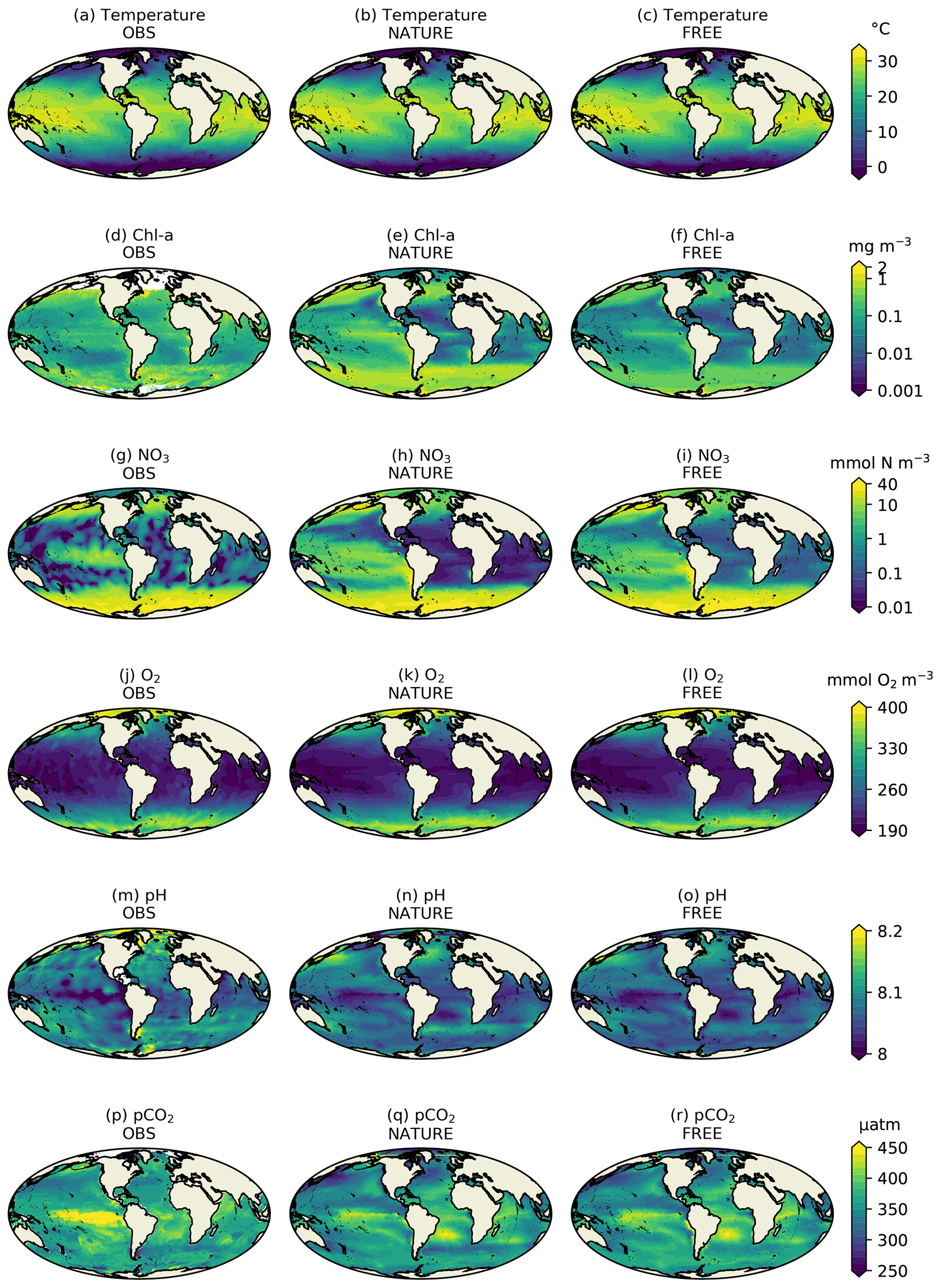
Figure 2Monthly mean surface (a–c) temperature, (d–f) Chl a, (g–i) NO3, (j–l) O2, (m–o) pH, and (p–r) pCO2 for December 2009 from real-world observation-based products (left column), NATURE (middle column), and FREE (right column).
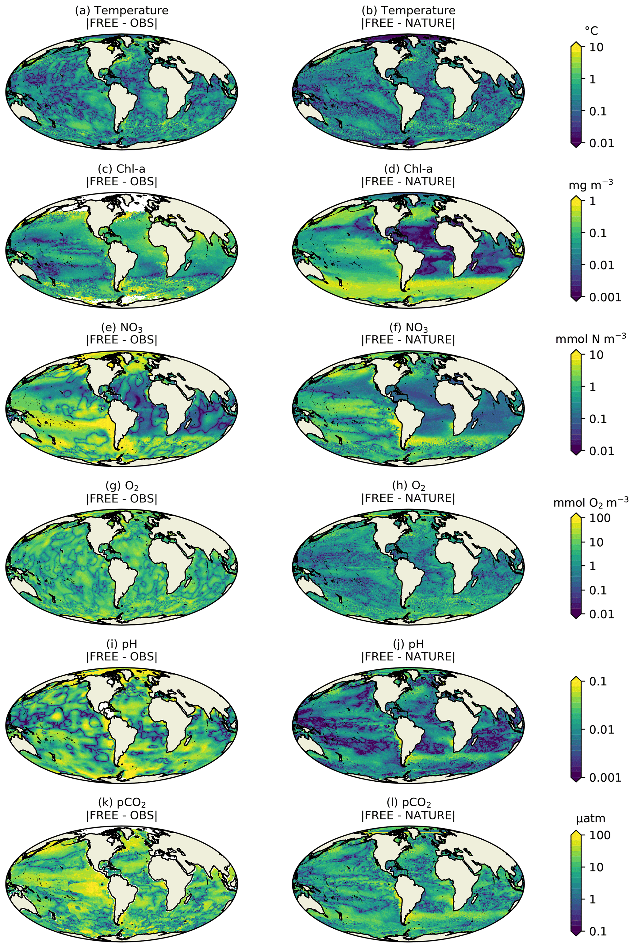
Figure 3Absolute difference for December 2009 for surface (a, b) temperature, (c, d) Chl a, (e, f) NO3, (g–h) O2, (i, j) pH, and (k, l) pCO2 between FREE and real-world observation-based products (left column), as well as between FREE and NATURE (right column).

Figure 4Annual zonal mean sections of (a–c) NO3, (d–f) O2, and (g–i) pH from real-world observation-based products (a, d, g), NATURE (b, e, h), and FREE (c, f, i).
3.1 Overview
As detailed by Masutani et al. (2010), OSSEs provide a way to test the impact on forecasts and reanalyses of assimilating observations which do not yet exist by using synthetic observations. An OSSE typically comprises the following elements:
-
a “nature run”, which is a realistic non-assimilative model simulation of the real world that provides a “truth” against which to validate the assimilative model;
-
synthetic observations representing both existing routine observations and future observing networks, which are sampled from the nature run with appropriate errors prescribed;
-
optionally, a free run, which provides an alternative model simulation of the nature run period;
-
an assimilative run, which assimilates synthetic observations representing existing routine observations into the alternative model simulation;
-
one or more additional versions of the assimilative run which also assimilate synthetic observations representing the future observing networks under consideration; and
-
assessment of the impact on reanalysis or forecast skill of assimilating these observations by validating against the nature run.
One of the keys to obtaining informative results from an OSSE is to ensure that all sources of error are appropriately accounted for (Halliwell et al., 2014, 2017; Hoffman and Atlas, 2016). If the free run is more similar to the nature run than the real forecasting system is to the real world, then it can become easier for the assimilative system to recover the truth, and the impact of the observing networks may be incorrectly estimated. As such, three general OSSE approaches have been developed, which differ in how the free run varies from the nature run.
-
In “identical twin experiments”, the nature and free runs differ only in their initial conditions. This set-up was frequently used in early OSSEs, but as most sources of model error are neglected, the results were found to be overly optimistic, and the approach is no longer widely recommended (Arnold and Dey, 1986).
-
In “fraternal twin experiments”, the same model is still used for both the nature and free run, but more aspects are modified. These could include the initial conditions, lateral and surface boundary conditions, parameterisations, and resolution. This takes much better account of model errors, and the approach is recommended over identical twin experiments (Arnold and Dey, 1986; Masutani et al., 2010; Yu et al., 2019).
-
In “full OSSEs”, significantly different models are used for the nature and free runs in order to make the two more independent. The nature run is often run either at higher resolution than the assimilative model or with significantly different parameterisations (Fujii et al., 2019). It is recommended to use this approach if possible (Masutani et al., 2010), but it relies on having two appropriately different models available, which is not always the case.
Due to the lack of availability of an appropriate alternative model for the nature run, it was decided within AtlantOS to take a fraternal twin approach for the biogeochemical OSSEs. This is sufficient to account for most sources of error, as long as any limitations of the approach are considered when drawing and acting upon conclusions.
3.2 Model formulation
The nature run in this study was run from 1 January 2008 to 31 December 2009 using the default parameterisations for the model versions used. This is intended to be the best available non-assimilative model representation of the real world. Validation of the general performance of the different system components can be found in the references given in Sect. 2, and validation of the nature run is presented in Sect. 4.1. Atmospheric boundary conditions were taken from the ERA-Interim reanalysis (Dee et al., 2011). Initial conditions for NEMO were taken from the end of a 30-year hindcast of GO6 (Storkey et al., 2018). Initial conditions for CICE were taken from a pre-operational trial of the FOAM v14 system. Initial conditions for MEDUSA were based on year 5000 of the initial ocean-only phase of the spin-up of UKESM1 for use in CMIP6 projections (Yool et al., 2020). As the UKESM1 spin-up was run at 1∘ resolution with pre-industrial atmospheric CO2 concentrations, the UKESM1 fields were interpolated to resolution, and the DIC and alkalinity fields were replaced by the contemporary model estimates used to initialise the resolution experiments in Ford (2020). To allow the model to settle, the first year of the nature run was treated as spin-up. The period was chosen to match OSSEs of the in situ physics observing system performed at the Met Office (Mao et al., 2020) and more widely as part of AtlantOS (Gasparin et al., 2019).
The free run was performed for the same period, including spin-up, but differed from the nature run in the following ways.
-
Atmospheric boundary conditions were taken from the JRA-55 reanalysis (Kobayashi et al., 2015).
-
NEMO initial conditions were taken from an earlier date (1 January 1999) of the hindcast of Storkey et al. (2018).
-
MEDUSA initial conditions were taken from an earlier year (1218) of the UKESM1 ocean-only spin-up, with DIC and alkalinity taken from the end of the non-assimilative resolution experiment of Ford (2020).
-
The NEMO parameter rn_efr, which affects near-inertial wave breaking and therefore vertical mixing (Calvert and Siddorn, 2013), was increased from 0.05 to 0.1.
-
The scheme used for advection of biogeochemical variables was changed from total variance dissipation (TVD) (Zalesak, 1979) to the monotone upstream scheme for conservative laws (MUSCL) (Van Leer, 1977; Lévy et al., 2001).
-
An alternative set of MEDUSA parameters was used, specifically parameter set 3 from Table 2 of Hemmings et al. (2015), which was found to give differences of an appropriate magnitude.
Together, these modifications generate approximations to the errors that exist in atmospheric fluxes and simulations of ocean physics and biogeochemistry. It is important to modify all of these, as errors in atmosphere and ocean physics have significant impacts on biogeochemical reanalyses and forecasts, and these errors must be accounted for if realistic conclusions are to be drawn from the OSSEs.
3.3 Synthetic observations
Synthetic ocean colour and BGC-Argo observations were generated from the nature run for each day of 2009. Total Chl a from ocean colour represents the current observing network typically assimilated in biogeochemical reanalyses (Fennel et al., 2019). Observations were simulated at the same locations that were actually observed in 2009 in version 3.1 of the ESA Climate Change Initiative (CCI) level 3 daily merged sinusoidal grid product (Sathyendranath et al., 2018, 2019), as used in recent Met Office reanalyses (Ford and Barciela, 2017). Whilst the products date from 2009 rather than the present day, the observational coverage is similar, with three sensors contributing in 2009 (MERIS, MODIS, and SeaWiFS) and three contributing to recent ocean colour products (MODIS, OLCI, and VIIRS). BGC-Argo float trajectories were based on Argo float trajectories (Argo, 2000) used for physics OSSEs within AtlantOS (Gasparin et al., 2019). These were generated using recent real Argo float trajectories, with modifications to ensure more even geographic coverage – for details see Gasparin et al. (2019). In this study, for testing the scenario equivalent to having biogeochemical sensors on all current standard Argo floats, the same “backbone” float trajectories were used as in the studies synthesised by Gasparin et al. (2019). For the scenario equivalent to having biogeochemical sensors on one in four Argo floats, these were subsampled using the last two digits of the float IDs. The geographic coverage in each case is shown in Fig. 1.
In data assimilation, two components of observation error are typically considered: measurement error and representation error (Janjić et al., 2018). Measurement error has been accounted for in this study by adding unbiased Gaussian noise to the nature run values at observation locations using standard deviations from the literature. A standard deviation of 30 % was agreed on within AtlantOS for Chl a from ocean colour, a value commonly used in assimilation studies (Pradhan et al., 2020). The same value was used for BGC-Argo Chl a profiles, consistent with Boss et al. (2008). For the remaining variables the values from Johnson et al. (2017) were used: 1 % for O2, 0.005 for pH, and 0.5 mmol m−3 for NO3. To avoid generating spuriously noisy profiles, a single value of Gaussian noise was calculated per profile rather than at every depth level. Where the standard deviations used were a percentage, this was calculated using the mean of the profile.
Representation error arises from observations and models representing differing spatial and temporal scales and processes. Since the nature and free runs were at the same resolution, this was accounted for in the same way as for the physics OSSEs in AtlantOS (Gasparin et al., 2019). For each profile, the equivalent nature run values were calculated either 3 d before or 3 d after, chosen at random. The difference between these and the truth value were taken to be the representation error and added to the observation values. The advantage of this approach is that representation error is higher in more variable regions, as would be expected in real-world data assimilation applications.
3.4 Error covariances
For assimilating ocean colour data, the monthly varying background and observation error standard deviations from Ford (2020) were used. To provide consistency between assimilating surface and in situ log 10(Chl a), these were also used for assimilating log 10(Chl a) from BGC-Argo.
For other variables, pre-existing error standard deviations were not available, so they were calculated for this study. Observation error standard deviations were set to a climatological constant equal to the average global observation error specified. These were fixed in time and specified as 0.638 mmol m−3 for NO3, 2.767 mmol m−3 for O2, and 0.006 for pH. Background error standard deviations were calculated using the Canadian Quick (CQ) method (Polavarapu et al., 2005; Jackson et al., 2008), which uses the variance of the difference between successive days of a free-running model simulation as a proxy for background error variance. Annual background error standard deviations were calculated from the output of the free run. The CQ method is known to underestimate the magnitude of the error standard deviations (Bannister, 2008), and the results in this study were considerably lower than the observation error standard deviations used. In order to give sufficient weight to the observations for the assimilation to be effective, the background error standard deviations were inflated. This was achieved by multiplying the gridded field of background error standard deviations for each variable by a constant so that the global mean background error standard deviation matched the observation error standard deviation used for that variable. This meant that on average, equal weight was given to the background and to the observations, but the ratio of background to observation error varied spatially based on the estimates from the CQ method. Once the system is fully functioning with real BGC-Argo data available, the background error estimates can be appropriately refined based on the errors in the real-world assimilative model and the actual distribution of BGC-Argo observations.
3.5 Experiments
Using these inputs, a set of assimilation experiments was performed in addition to the nature and free runs, as detailed in Table 1. The nature and free runs were run from 1 January 2008 to 31 December 2009, with the first year treated as spin-up. Each assimilation experiment was run from 1 January 2009 to 31 December 2009 using initial conditions from the end of the free run spin-up and assimilating the synthetic observations into the version of the model used for the free run.
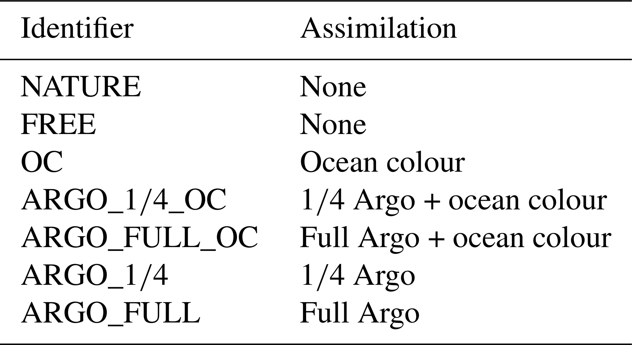
Five assimilation experiments were run. One just assimilated ocean colour. Two assimilated ocean colour in combination with the 1∕4 subsampled BGC-Argo array and the full BGC-Argo array. A final two runs assimilated the 1∕4 subsampled and full BGC-Argo arrays without ocean colour.
All the experiments, with unique identifiers for each, are detailed in Table 1.
3.6 Metrics
The main metrics used for assessment are the absolute and percentage reduction in median absolute error (MAE), respectively defined as
where MAEOSSE is the MAE of each OSSE compared with NATURE, and MAEcontrol is the MAE of a control run compared with NATURE. When considering the impact of data assimilation vs. a free run, FREE is used as the control run, and when assessing the added value of BGC-Argo over ocean colour, OC is used as the control run. A positive value of MAEred_abs or MAEred_% represents a reduction in error in the OSSE compared to the control, and a negative value represents an increase in error. This is a modification of the approach taken by Gasparin et al. (2019), who used the percentage reduction in mean square error. MAE is used instead because the biogeochemical variables being considered are highly non-Gaussian, so it is more appropriate to use a metric such as MAE, which is based on robust statistics. MAEred_abs is used in addition to MAEred_%, as this can be more informative in regions where MAEcontrol is small.
Where MAEred_abs or MAEred_% is presented as a spatial map, the MAE was calculated independently for each model grid cell. This was done by calculating the absolute difference between the model run and the nature run in that grid cell on each day of the given time period and calculating the median of those values. Where MAEred_abs or MAEred_% is presented as a profile, the MAE was calculated independently for each model depth level. At each depth, the absolute difference between the model run and the nature run on each day of the given time period was calculated for each grid cell in the region of interest. The median of this set of values was calculated, weighted by the area of each grid cell, to give the MAE value for that depth level.
The results are presented in two subsections below. The first assesses the ability of NATURE to capture key ocean features and how differences between NATURE and FREE compare to errors in real-world reanalyses. The second assesses the assimilation runs and the potential impact of assimilating BGC-Argo and ocean colour data.
4.1 Errors in free-running model
As stated in Sect. 3, OSSEs yield the most reliable conclusions when all sources of real-world error have been appropriately accounted for (Halliwell et al., 2014). This means that the errors between FREE and NATURE should, ideally, be broadly similar to the errors between FREE and the real world. Furthermore, NATURE should be able to represent key features observed in the real ocean. As the real-world ocean is not known exactly, observation-based products must be used to perform this assessment, even though these can have large uncertainties and do not exactly represent the real world. For many biogeochemical variables, coarse climatologies are the only suitable products for a global assessment.
Figure 2 shows surface fields of temperature, Chl a, NO3, O2, pH, and pCO2 from observation-based products, NATURE, and FREE. These are plotted for the final month of the simulations, December 2009, which is when the largest cumulative impact from the data assimilation will be seen. The observation-based products used are the EN4.2.1 monthly analysis product for temperature (Good et al., 2013; Gouretski and Reseghetti, 2010), the Ocean Colour CCI v3.1 monthly product for Chl a (Sathyendranath et al., 2018, 2019), the 2018 World Ocean Atlas (WOA18) monthly climatology for NO3 and O2 (Garcia et al., 2018a, b), the GLODAP v2 annual climatology for pH (Key et al., 2015; Lauvset et al., 2016), and the monthly statistical analysis product of Landschützer et al. (2015a, b) for pCO2. The observation-based products were bilinearly interpolated to the model grid.
For both physical and biogeochemical variables, NATURE captured the broad global distribution, with generally appropriate magnitudes. There were some discrepancies, such as an overestimation of Chl a in parts of the Pacific and Southern Ocean and an underestimation in the Atlantic and Indian Ocean. NO3 was too low in the Atlantic and Indian Ocean, and pCO2 was too low in the tropical Pacific. Overall though, NATURE matched the observation-based products sufficiently well for it to be used as the truth in these experiments.
FREE also broadly captured these features, as expected from state-of-the-art models (Fennel et al., 2019). Differences between FREE and NATURE were generally similar to the differences between FREE and the observation-based products, but there are some exceptions. This can be seen more clearly in Fig. 3, which shows the absolute difference between FREE and the observation-based products and between FREE and NATURE for the fields plotted in Fig. 2.
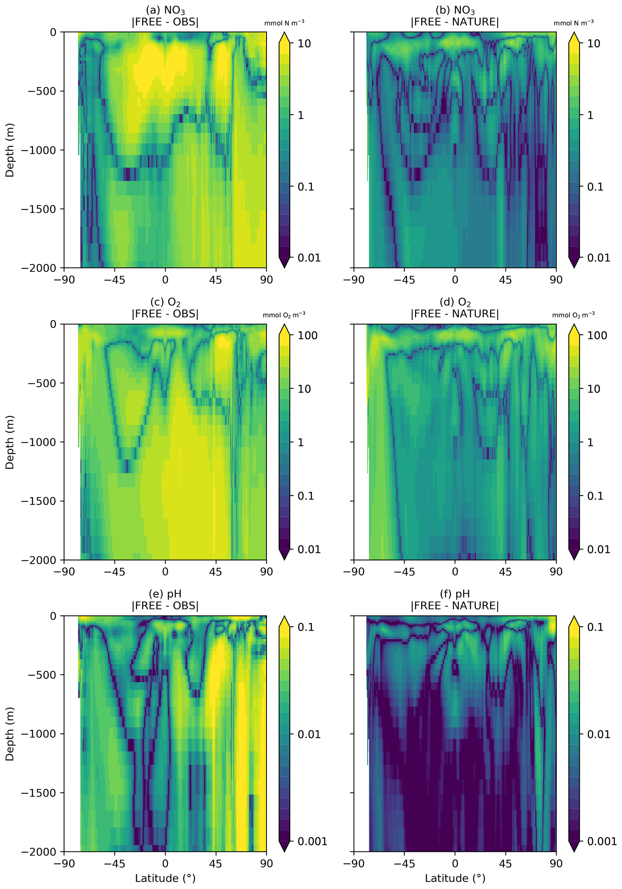
Figure 5Absolute difference between FREE and real-world observation-based products (a, c, e) and between FREE and NATURE (b, d, f) for annual zonal mean sections of (a, b) NO3, (c, d) O2, and (e, f) pH.
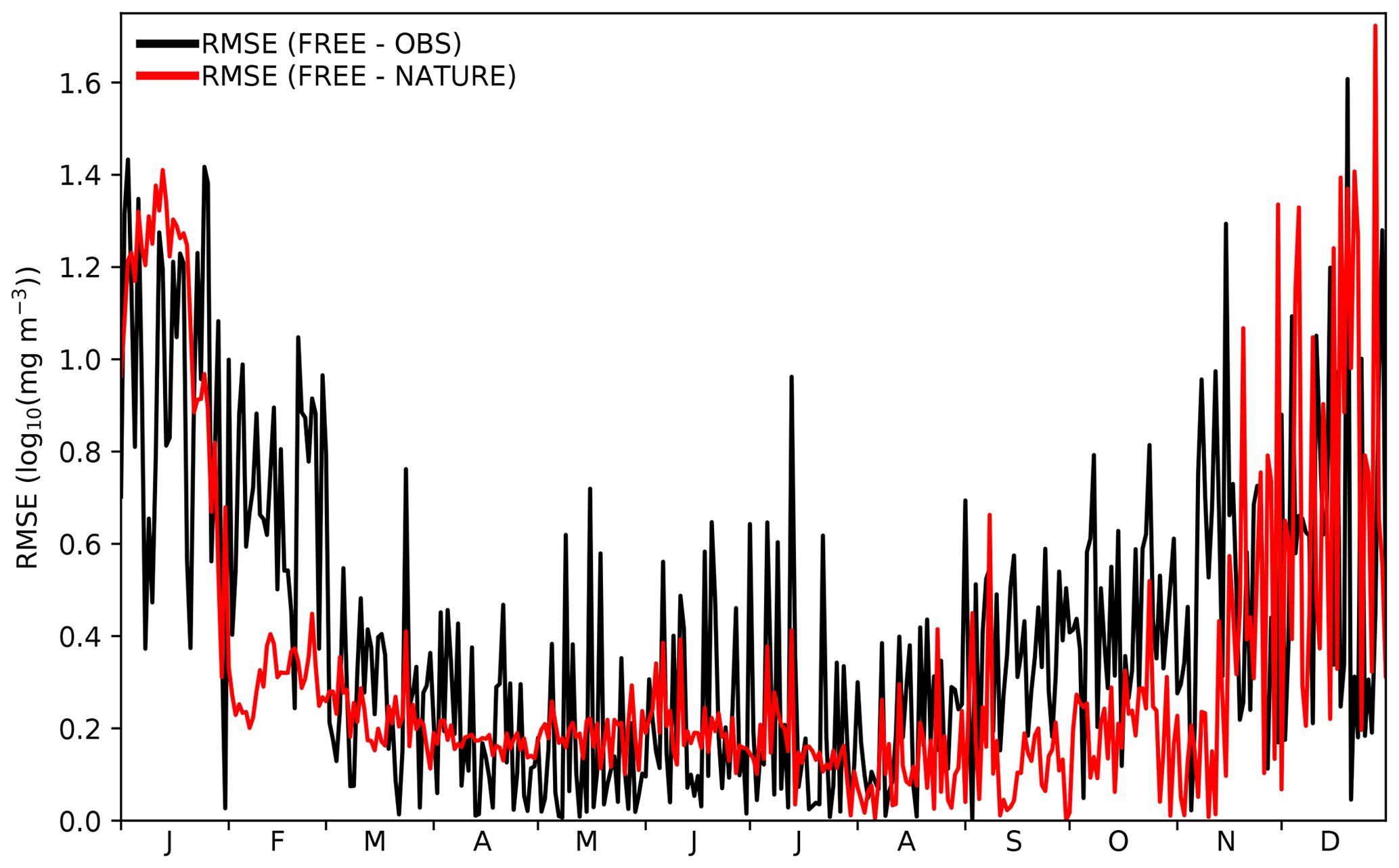
Figure 6Time series of daily global RMSE for surface log 10(Chl a) between FREE and CCI ocean colour observations (black line) and between FREE and NATURE (red line) at CCI ocean colour observation locations.
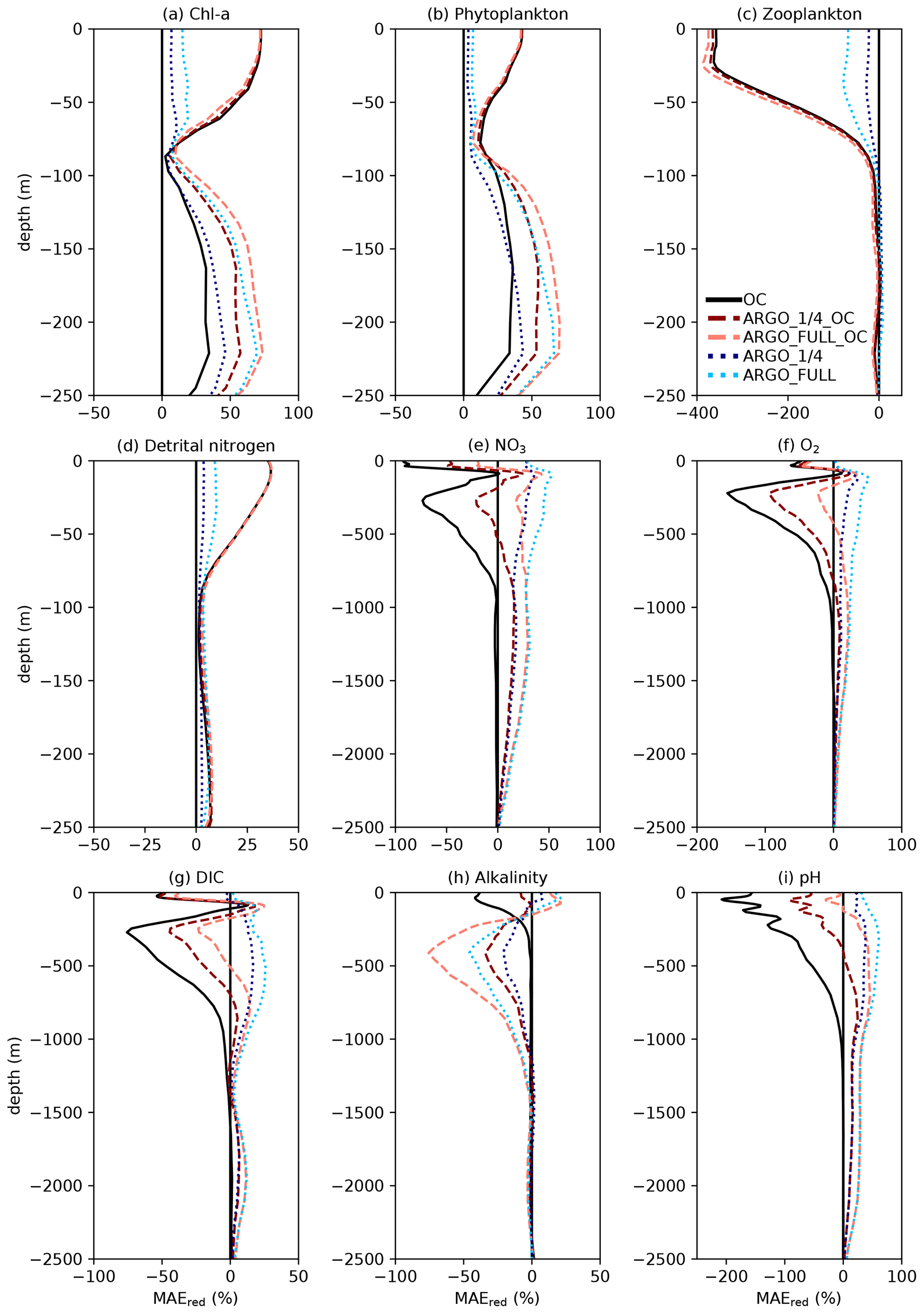
Figure 7Profiles of global MAEred_% over FREE for December 2009. Note that axis scales differ between subplots.
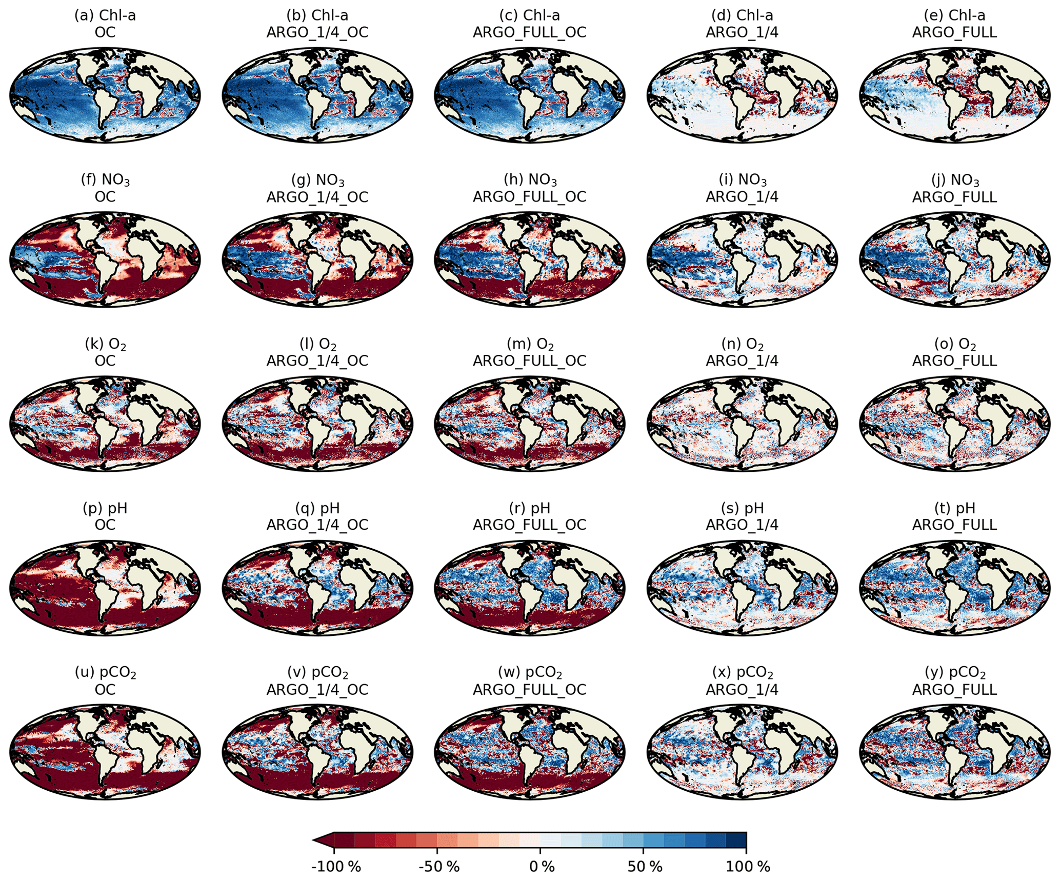
Figure 8Surface MAEred_% over FREE for Chl a, NO3, O2, pH, and pCO2 for December 2009.
For temperature (Fig. 3a, b), the absolute difference between FREE and NATURE was very similar in pattern to that between FREE and the EN4 analysis but slightly lower in magnitude in some regions. This suggests that the perturbations applied to the physics (different atmospheric fluxes, initial conditions, and vertical mixing) resulted in an error contribution to the biogeochemical model similar to, but slightly smaller than, that seen in state-of-the-art modelling systems. For Chl a (Fig. 3c, d), the two sets of absolute difference were broadly similar in the Pacific and Southern Ocean, but in the tropical Atlantic and Indian Ocean the absolute difference between FREE and NATURE was smaller than between FREE and the CCI data. In NATURE the Chl a in these regions was too low compared with observations, linked to low nutrient concentrations (Fig. 2). The modifications introduced in FREE served to increase nutrient concentrations in these regions but also to suppress phytoplankton growth, resulting in little overall change in Chl a. This is largely the result of increasing the nitrogen nutrient uptake half-saturation concentration for phytoplankton and decreasing the zooplankton grazing half-saturation concentration. Elsewhere though, the levels of absolute error were broadly similar, meaning the OSSEs had realistic levels of model error. For NO3, O2, pH, and pCO2 (Fig. 3e–l), the global distributions of absolute error were generally similar between FREE and NATURE and between FREE and the observation-based products, although the absolute difference between FREE and NATURE was often smaller. It should be remembered though that the observation-based products used here have large uncertainties themselves. Furthermore, NATURE is the truth and therefore error-free.
A similar comparison is required for the subsurface ocean, as BGC-Argo profiles were simulated for the upper 2000 m. Fewer observation products are available for such an assessment. No subsurface climatology is available for Chl a, and only annual climatologies covering the full water column are available for NO3 and O2 from WOA18 and for pH from GLODAP v2. Annual zonal mean sections of NO3, O2, and pH are therefore plotted for the upper 2000 m in Fig. 4 from the observation-based products, NATURE, and FREE. For all three variables, NATURE captured the broad zonal and depth variations of the climatologies well, with appropriate magnitudes. NO3 concentrations in the upper 1000 m were slightly too high in the low and middle latitudes, as were O2 and pH below 500 m, but there were no major discrepancies. FREE also captured the observed distributions of all three variables, though differences between FREE and NATURE were often slightly smaller than between FREE and the observation-based products, as shown in Fig. 5.
A further consideration is that the growth of errors with time between FREE and NATURE should be comparable to that between FREE and real-world observations (Halliwell et al., 2014). The only assimilated variable for which there are sufficient daily observations to assess this is Chl a from ocean colour. In Fig. 4 time series of root mean square error (RMSE) for surface log 10(Chl a) are plotted between FREE and NATURE and between FREE and observations. The observations are the daily CCI data used to define the locations of the synthetic ocean colour observations. For the comparison, model values were bilinearly interpolated to the observation locations, and a daily global RMSE value calculated. The magnitude of the RMSE between FREE and NATURE and between FREE and the observations was very similar and remained comparable throughout the year, with higher RMSE in austral summer in both cases. The RMSE variability was typically smaller between FREE and NATURE though, suggesting this to be a source of error not fully captured in FREE.
While it is not ideal that the Chl a errors differ in the tropical Atlantic and Indian Ocean, and errors between FREE and NATURE were too low for some variables, achieving globally appropriate levels of error with a complex biogeochemical model with globally uniform parameterisations could not be managed within the resources of the project. Furthermore, the similarity of Chl a between NATURE and FREE in some regions was due to the introduction of compensating errors in FREE rather than a lack of model error. This itself is a common feature of reanalyses, which can result in data assimilation increasing overall error by correctly reducing one of a set of compensating errors, as demonstrated by Ford and Barciela (2017). For regions and variables for which the errors between FREE and NATURE were too low, the potential result may be to underestimate the impact of assimilating dense data, in this case ocean colour, and overestimate the impact of assimilating sparse data, in this case BGC-Argo (Halliwell et al., 2014). This should be borne in mind when drawing conclusions.
4.2 Assimilation runs
For each of the five assimilation runs, profiles of global MAEred_% over FREE for December 2009 are plotted in Fig. 7 for nine model variables. The results for MAEred_abs are very similar to those for MAEred_% (not shown). For Chl a (Fig. 7a), phytoplankton biomass (Fig. 7b), zooplankton biomass (Fig. 7c), and detrital nitrogen (Fig. 7d), which only have significant concentrations in the euphotic zone, profiles are plotted for the upper 250 m. For NO3 (Fig. 7e), O2 (Fig. 7f), DIC (Fig. 7g), alkalinity (Fig. 7h), and pH (Fig. 7i), profiles are plotted for the upper 2500 m. Recall that Chl a, NO3, O2, and pH observations, assimilated in the BGC-Argo experiments, were produced for the upper 2000 m.
For Chl a, OC, ARGO_1∕4_OC, and ARGO_FULL_OC all had an MAEred_% value of 72 % at the surface. This suggests that ocean colour was very successful at improving surface Chl a, while BGC-Argo was unable to add much information to that gained from the much denser ocean colour observations, at least at the global scale. When only BGC-Argo was assimilated, a small improvement at the surface of 7 % and 15 % was seen in ARGO_1∕4 and ARGO_FULL, respectively. Beneath the surface, at depths likely to see a deep chlorophyll maximum, BGC-Argo had much greater impact, with all four runs outperforming OC. ARGO_FULL outperformed ARGO_1∕4, demonstrating benefit from extra in situ observations. Combining BGC-Argo and ocean colour gave better results at this depth in ARGO_1∕4_OC (which is the proposed observing system), but ARGO_FULL and ARGO_FULL_OC performed similarly. Beneath the euphotic zone, where Chl a was near zero, the assimilation had little impact. Positive values of MAEred_% were seen below 250 m, but values of MAEred_abs (not shown) tended to zero below about 220 m.
The results for phytoplankton biomass were very similar to those for Chl a. For zooplankton biomass, which was not directly updated by the assimilation, a large degradation in surface values was seen in all three runs assimilating ocean colour data, with the impact reducing to near zero at around 100 m. A smaller degradation was seen in ARGO_FULL that was reduced further in ARGO_1∕4. Detrital nitrogen was improved in the upper 100 m in all runs, especially those assimilating ocean colour, with little absolute impact of the assimilation beneath that depth.
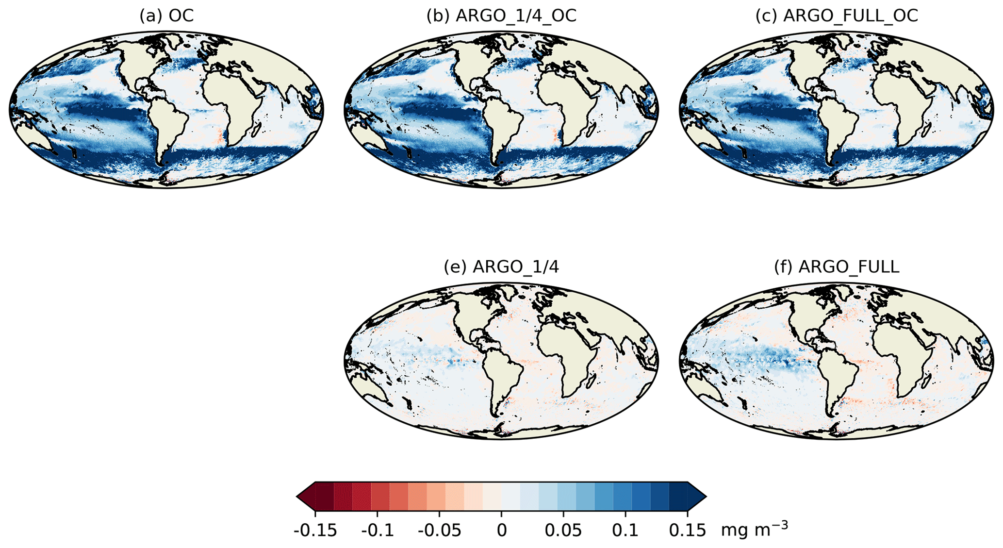
Figure 9Surface MAEred_abs over FREE for Chl a for December 2009.
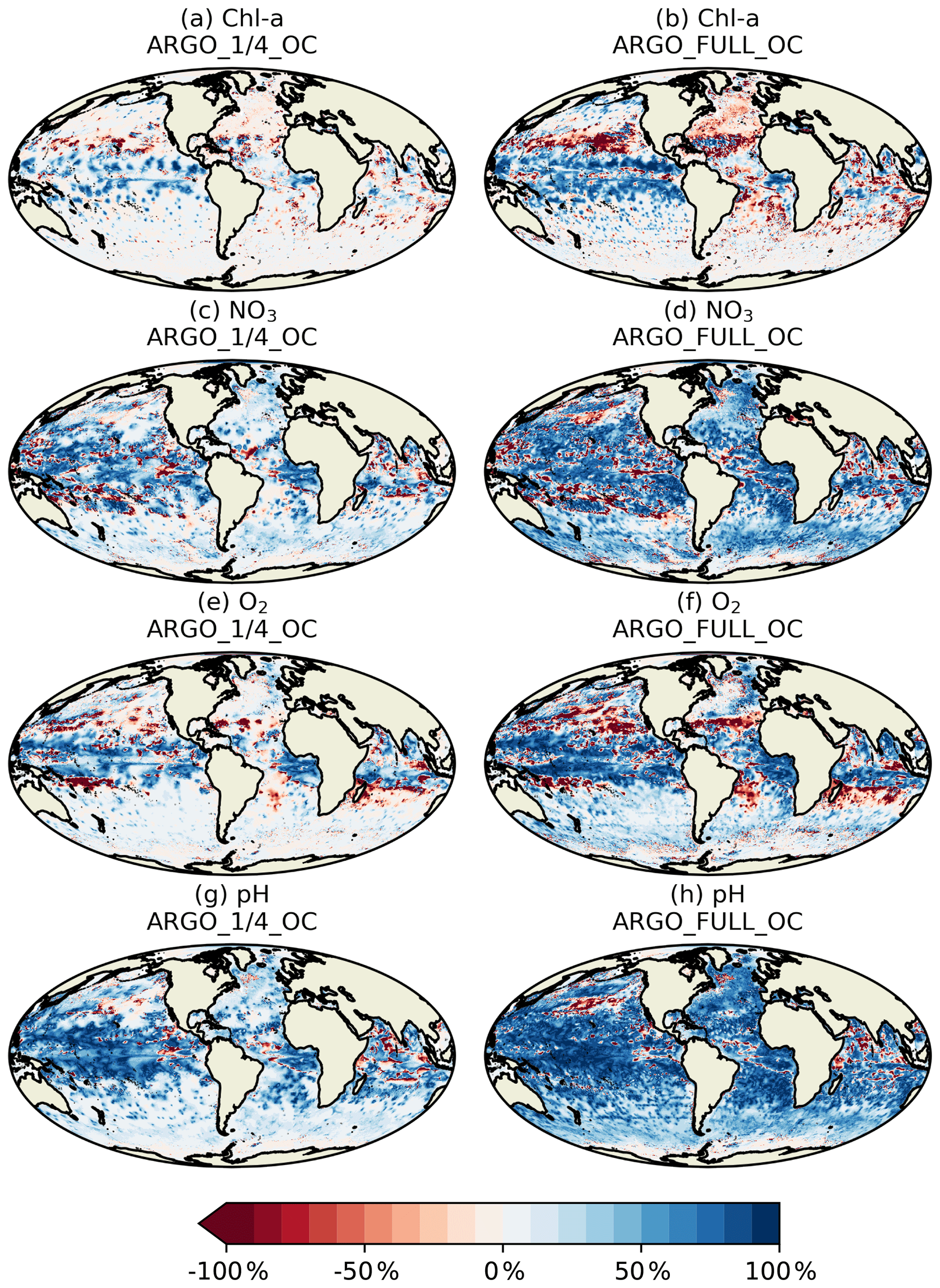
Figure 10MAEred_% over OC for Chl a, NO3, O2, and pH for December 2009 at 100 m of depth.
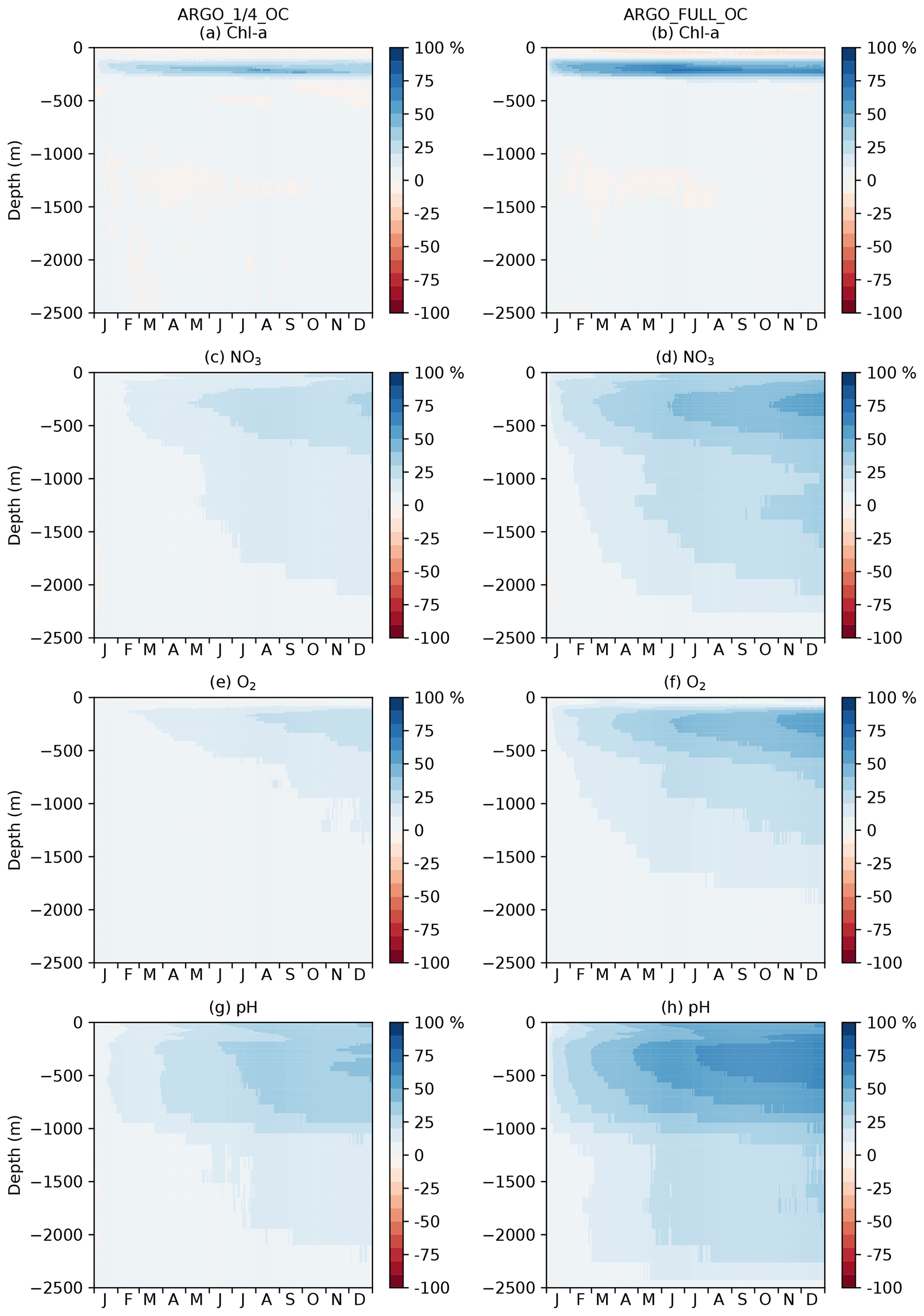
Figure 11Hovmöller diagram of daily global MAEred_% over OC with depth for Chl a, NO3, O2, and pH.
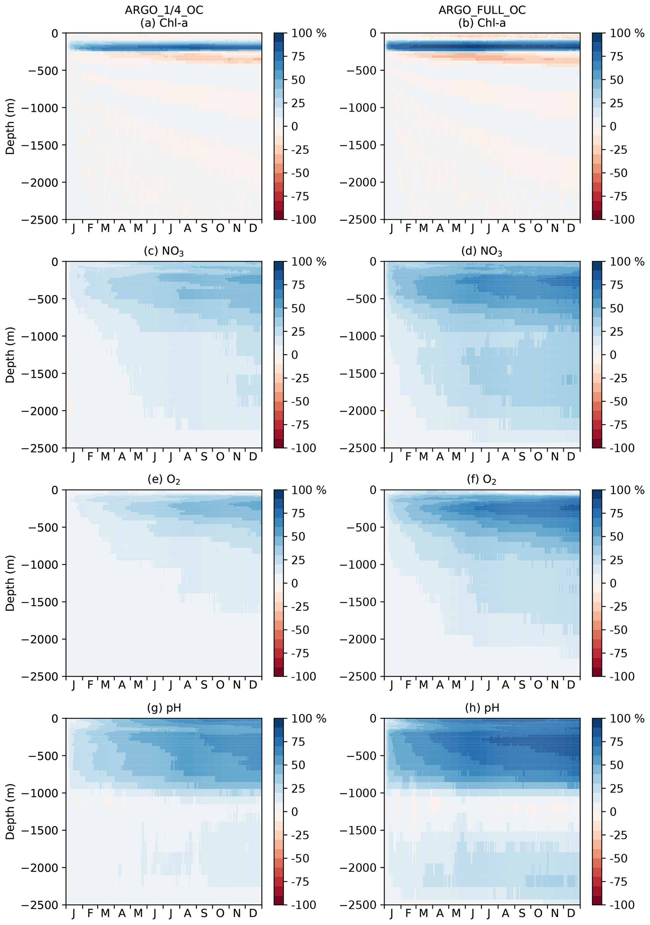
Figure 12Hovmöller diagram of daily MAEred_% over OC with depth in the tropical Pacific for Chl a, NO3, O2, and pH.
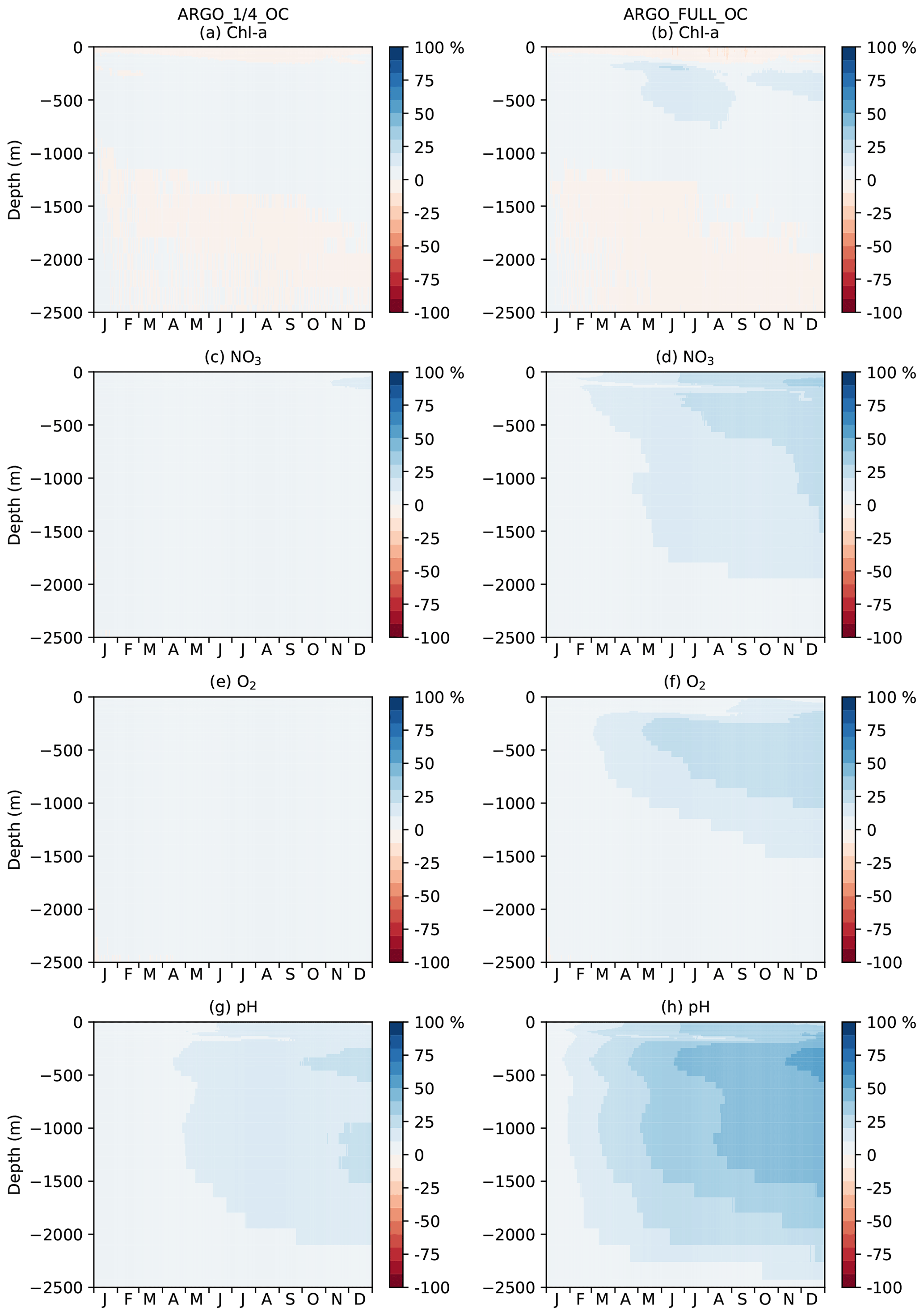
Figure 13Hovmöller diagram of daily MAEred over OC with depth in the Southern Ocean for Chl a, NO3, O2, and pH.
For NO3 and O2, which were assimilated from the BGC-Argo floats, there was a clear improvement throughout the water column to 2500 m in ARGO_1∕4 and ARGO_FULL, with greater improvement when more floats were assimilated. Maximum MAEred_% was seen at 100–120 m of depth, with less of an impact at the surface, particularly for O2. In OC, NO3 and O2 were degraded in the upper 1000 m. Adding BGC-Argo to ocean colour assimilation partially mitigated this, with positive MAEred_% at some depths and negative MAEred_% at others.
With the carbon cycle, DIC, alkalinity, and pH were all degraded in OC. In ARGO_1∕4 and ARGO_FULL, throughout most of the water column DIC was improved and alkalinity degraded, with an overall improvement in the assimilated variable pH. Combining ocean colour and BGC-Argo assimilation gave mixed results, with a degradation in pH in the surface layers but an improvement at depth.
Spatial maps of surface MAEred_% over FREE for December 2009 are plotted in Fig. 8 for the five assimilation runs for Chl a, NO3, O2, pH, and pCO2. In OC surface Chl a was almost universally improved (Fig. 8a), apart from a few small areas in the Atlantic, North Pacific, and Indian Ocean. These correspond to areas where NATURE and FREE were almost identical, as seen in Fig. 3d, so the observation errors were larger than the model error. Very little difference was made by adding BGC-Argo to ocean colour assimilation, while assimilating just BGC-Argo data gave mixed results for Chl a at the surface. In the Pacific Ocean, Chl a was slightly improved in ARGO_1∕4 and further improved in ARGO_FULL, while in the Atlantic and Indian Ocean a degradation was seen. This again corresponds to regions where there was little absolute difference between NATURE and FREE (Fig. 3d). As such, MAEred_% is not the most informative metric in these regions, and it is more appropriate to examine MAEred_abs. This is plotted for Chl a in Fig. 9, which shows the absolute value of the degradation to be very small.
Surface NO3 was degraded almost everywhere in OC (Fig. 8f), apart from the tropical Pacific, which is where some of the largest differences were seen between NATURE and FREE (Fig. 3f). Adding BGC-Argo assimilation increased this improvement and started to reverse the degradation in other regions, particularly in ARGO_FULL_OC. Assimilating just BGC-Argo improved NO3 in most areas, with more impact seen with more floats, but the results were patchy in places.
The story for O2 (Fig. 8k–o) was very similar to that for NO3 but with a smaller degradation introduced by ocean colour assimilation and a smaller improvement brought about by BGC-Argo assimilation. For pH (Fig. 8p–t) and pCO2 (Fig. 8u–y), the patterns were also similar but with a greater degradation introduced by ocean colour assimilation and a greater improvement brought about by BGC-Argo assimilation. Improvements to DIC and alkalinity when assimilating pH should also help improve pCO2, which was not directly assimilated, though the details of the impact differ between the two variables.
Current state-of-the-art reanalyses typically assimilate ocean colour data (Fennel et al., 2019), so to demonstrate the additional impact BGC-Argo might have in these systems, the remainder of this section focusses on MAEred_% over OC rather than over FREE. Spatial plots of MAEred_% over OC for December 2009 at 100 m of depth are shown in Fig. 10 for the assimilated variables Chl a, NO3, O2, and pH. Clear benefit was found for all variables, with greater improvements than at the surface. The improvement was largest for pH and smallest for Chl a, and in all cases a greater impact was seen in ARGO_FULL_OC than ARGO_1∕4_OC.
To investigate the impact of the BGC-Argo assimilation over the full year, a Hovmöller diagram (Hovmöller, 1949) of daily global MAEred_% over OC with depth is plotted for each of the assimilated variables for ARGO_1∕4_OC and ARGO_FULL_OC in Fig. 11. For Chl a (Fig. 11a, b), ARGO_1∕4_OC and ARGO_FULL_OC both displayed a very small degradation compared with OC in the surface layers throughout the year. This is consistent with the small difference seen between the runs in the profiles in Fig. 7a. Between about 80 and 300 m of depth, where deep chlorophyll maxima may be found, a strong positive impact was found on Chl a, which was strongest in ARGO_FULL_OC. In both runs this took a few weeks to spin up, then remained reasonably consistent throughout the year. Beneath about 300 m of depth, values of MAEred_% were near zero, as Chl a was negligible. For NO3, O2, and pH, an almost universal improvement was seen throughout the water column. For all three variables, values of MAEred_% were highest in the upper 1000 m, with a maximum at a similar depth or slightly deeper than that for Chl a. MAEred_% was consistently higher in ARGO_FULL_OC than in ARGO_1∕4_OC, again demonstrating a positive impact from having a greater number of BGC-Argo floats. In both runs, MAEred_% increased throughout the year, suggesting that the impact of the assimilation was still spinning up, and the full potential would not be realised until the system had been run for longer than a year.
In Fig. 11, global MAEred_% is shown. As can be seen in Fig. 10, the subsurface impact of the BGC-Argo assimilation was not globally uniform, with a stronger impact typically seen at low latitudes than at high latitudes. To demonstrate this further, equivalent versions of Fig. 11 are shown for the tropical Pacific in Fig. 12 and for the Southern Ocean in Fig. 13. In the tropical Pacific, the patterns for all the assimilated variables were very similar to the global average but with higher MAEred_% values, showing a stronger positive impact of the assimilation. This was especially large for Chl a between 80 and 300 m of depth and pH in the upper 1000 m. MAEred_% values for Chl a were largely negative below 300 m, but MAEred_abs values were near zero (not shown) due to Chl a concentrations being negligible. For NO3, O2, and pH, the impact of the assimilation was still spinning up after a year. In the Southern Ocean, MAEred_% values were much lower, with an especially limited impact from the BGC-Argo assimilation in ARGO_1∕4_OC. MAEred_% was typically largest for pH and lowest for Chl a. The impact of the assimilation continued to increase with time, so it may have just been taking longer to spin up than at lower latitudes. Similar results were seen in the Arctic Ocean (not shown). Increments also spread further in tropical regions due to longer correlation length scales and faster propagation timescales.
A set of observing system simulation experiments (OSSEs) was performed to explore the impact on global ocean biogeochemical reanalyses of assimilating currently available ocean colour data and assess the potential impact of assimilating BGC-Argo data. Two different potential BGC-Argo array distributions were tested: one for which biogeochemical sensors are placed on all current Argo floats and one for which biogeochemical sensors are placed on a quarter of current Argo floats. This latter approximately corresponds to the proposed BGC-Argo array of 1000 floats (Roemmich et al., 2019). Assimilating the synthetic ocean colour data greatly improved the assimilated variable surface Chl a but had a mixed impact on the wider ecosystem and carbon cycle. Assimilating the synthetic BGC-Argo data gave no added benefit over ocean colour in terms of simulating surface Chl a, but for most other variables, including subsurface Chl a, adding BGC-Argo improved results throughout the water column. This included surface pCO2, which was not assimilated but is an important output of reanalyses. Both BGC-Argo array distributions gave benefits, with greater improvements seen with increased numbers of observations. The impact of the BGC-Argo assimilation also increased with time and had not yet fully spun up after a year.
Real-world experiments assimilating Chl a from ocean colour have widely found benefits when validating surface Chl a against independent observations (Gehlen et al., 2015; Fennel et al., 2019), a conclusion echoed in this study. The impact of ocean colour assimilation on the wider model state has always been more ambiguous, with various studies reporting largely neutral or sometimes negative results and some evidence of positive impacts highlighted (e.g. Gregg, 2008; Ciavatta et al., 2011; Fontana et al., 2013; Ford and Barciela, 2017). The sparsity of in situ observations, especially for variables such as phytoplankton and zooplankton biomass, has always made it difficult to validate results or compare conclusions from different studies. Many studies have used inherently multivariate assimilation methods such as the ensemble Kalman filter (Evensen, 2003), while others have employed balance relationships (Ford et al., 2012; Rousseaux and Gregg, 2012; Teruzzi et al., 2014; Skákala et al., 2018). This study used a form of the latter, with phytoplankton biomass variables updated to maintain background stoichiometric ratios. Updating phytoplankton biomass, a simple extra step which improved phytoplankton biomass itself and should therefore be expected to improve other model variables, resulted in a degradation of all other variables examined except for detritus. Zooplankton biomass was especially affected. It seems likely that this degradation occurred due to the changed MEDUSA parameter settings between NATURE and FREE, meaning that the underlying processes were altered such that identical concentrations of phytoplankton now led to different concentrations of other variables. Relevant perturbations included changes to the grazing half-saturation concentration for zooplankton and nutrient uptake half-saturation concentrations for phytoplankton. This suggests that unless a given biogeochemical model can accurately describe all relevant biogeochemical processes in the ocean, which has not yet been demonstrated, simply improving phytoplankton concentrations might be as likely to degrade as improve other variables. This will also be the case for assimilation schemes which use ensembles to generate cross-correlations between Chl a and other model variables. These schemes are reliant on the model relationships between variables being correct, as it is these model relationships which the cross-correlations are based on. If the response of zooplankton to an increase in phytoplankton in the model ensemble differs from that in the real ocean, then the cross-correlations used in the assimilation will lead to a zooplankton response which follows the (incorrect) model rather than the real ocean in exactly the same way as seen in this study. An alternative approach could be to use the nitrogen balancing scheme of Hemmings et al. (2008), which explicitly updates several model state variables to try and account for differing errors in phytoplankton growth and loss processes. This has been successfully used in previous ocean colour assimilation studies (Ford et al., 2012; Ford and Barciela, 2017; Ford, 2020) with the HadOCC model (Palmer and Totterdell, 2001). It was originally designed and tuned for use with HadOCC, so it requires further development and tuning for use with the more complex MEDUSA, but an initial implementation for MEDUSA has been developed. Such a scheme offers more potential for controlling the wider biogeochemical state, especially if it could be expanded to alter parameter values in addition to state variables.
Adding assimilation of BGC-Argo profiles of Chl a, NO3, O2, and pH brought clear improvements to all assimilated variables and some unassimilated ones. The impact was increased with a larger BGC-Argo array, suggesting that benefits may be seen up to and beyond the target array size of 1000 floats. The observations added important subsurface information which cannot be obtained from satellite data but which can yield improvements in simulations of variables such as air–sea CO2 fluxes. All assimilated variables were greatly improved below the mixed layer. The greatest improvement was in terms of Chl a around the nitracline at depths where deep chlorophyll maxima are likely to be found. This should help quantify a major contributor to global primary production, which cannot be observed from space. At the surface, more limited improvements were seen for Chl a and O2 than for NO3 and pH. This is likely due to the relative importance of different physical processes affecting these variables and the density of data required for the assimilation to have a major impact. In the case of NO3 and DIC, which helps control pH, concentrations typically increase with depth, and the supply of NO3 and DIC from below the mixed layer is a major contribution to surface values. Therefore, changes at depth due to the assimilation will alter surface values through indirect processes. O2 and Chl a typically decrease in concentration with depth, and dynamics within the mixed layer are much more important in setting surface values. For O2, major drivers are temperature and ocean–atmosphere exchange. For Chl a a major driver is light availability. It seems that the BGC-Argo data was too sparse, even in ARGO_FULL, to have a widespread impact in these circumstances. More dedicated observations within the mixed layer may be likely to have more of an impact on surface values. For Chl a, this can be successfully provided by ocean colour, as the results of this study show. For O2 and other variables, alternative in situ observing technologies such as gliders may be able to play a role (Telszewski et al., 2018). It should be noted, though, that the OSSE framework used here did not consider possible real-world issues such as observation biases and inconsistencies between ocean colour and BGC-Argo Chl a observations. Furthermore, for some variables and regions the error between the free-running model and the nature run was smaller than might be expected in real-world systems, potentially leading to an overestimate of the quantitative impact of BGC-Argo data (Halliwell et al., 2014).
For NO3, O2, and pH, the overall impact of the assimilation increased with time and appeared to still be spinning up after a year. The likely explanation is that increments from individual BGC-Argo floats only influenced a relatively small local area, but this influence was long-lasting. Therefore, as further increments in different locations were added with time, the overall error of the system continued to decrease. This suggests that the BGC-Argo observations will take some time to show their full benefit for assimilation, a greater number of floats will be required, or changes to the assimilation method will be required to make better use of sparse observations. For Chl a, which is typically more dynamic, this appeared to be less of an issue.
There is much scope for improving data assimilation methodologies to better use existing satellite data and sparse in situ observations, which could bring at least as much benefit as expanding observing systems. Multivariate balancing and better integration with physics data assimilation may help improve unassimilated variables. More effective ways of spreading information from sparse data, such as cross-covariances based on empirical orthogonal functions or derived from an ensemble assimilation scheme, should also be considered. Related to this, the correlation length scales used by the assimilation should be appropriately tuned for biogeochemical variables. In this study, a single horizontal correlation length scale based on the first baroclinic Rossby radius was used, varying from a value of 25 km at low latitudes to 150 km at the Equator, following the physics implementation of Waters et al. (2015). This may help explain why the BGC-Argo assimilation demonstrated less of a widespread impact at high latitudes than near the Equator. A different correlation length scale may be appropriate for biogeochemical variables. Furthermore, NEMOVAR has recently been developed to allow the use of multiple correlation length scales (Mirouze et al., 2016), so both small- and large-scale corrections can be considered. The background error standard deviation estimates also need to be refined once real BGC-Argo observations are being assimilated to reflect the background error in the assimilative system, which will depend on the actual distribution of BGC-Argo floats. The average ratio of background to observation error may also differ from that assumed in this study. It is likely that this would give different quantitative results, but the qualitative impact of the assimilation would remain similar.
A novel method for assimilating pH was introduced in this study, following the method for assimilating pCO2 developed by While et al. (2012). The method corrects pH, a diagnostic variable in the model, by making the smallest combined change to DIC and alkalinity required to reach the target pH value. This was successful in improving both pH and DIC, but alkalinity was often degraded. This highlights the fact that making the smallest combined change to DIC and alkalinity does not guarantee that errors in both DIC and alkalinity are minimised. In some circumstances it might be more appropriate to make a smaller or no change to alkalinity and a larger change to DIC or even to make a change of the opposite sign to alkalinity and an even larger change to DIC to compensate. Unfortunately, without concurrent observations of DIC or alkalinity, this information is not known at the time of assimilation. This is equally the case whether pCO2 or pH is being assimilated, so it was decided that the safest assumption would be to make the smallest combined change to DIC and alkalinity. In light of these results it may be worth revisiting this assumption.
From the point of view of ocean data assimilation, BGC-Argo will bring significant advances in reanalysis and forecasting skill, and it is recommended to proceed with its development as a priority. The proposed array of 1000 floats will be enough to deliver clear improvements, and a larger array would be likely to bring further benefits. Ocean colour and BGC-Argo provide complementary information, so maintaining and developing the existing ocean colour satellite constellation should also be a priority. Technologies such as gliders may also bring additional benefits, for instance for O2 in the mixed layer.
The nature of the 4-D data generated in running the model experiments requires a large tape storage facility. These data are in excess of 100 terabytes (TB). However, the data can be made available upon request from the author.
The author declares that there is no conflict of interest.
This article is part of the special issue “Biogeochemistry in the BGC-Argo era: from process studies to ecosystem forecasts (BG/OS inter-journal SI)”. It is not associated with a conference.
The author would like to thank Susan Kay and Matt Martin for useful discussions and comments on the draft paper, as well as the two anonymous reviewers for their helpful comments in the Biogeosciences discussion forum. This study used synthetic observations based on Argo data. These data were collected and made freely available by the International Argo Program and the national programmes that contribute to it (http://www.argo.ucsd.edu, http://argo.jcommops.org, last access: 14 October 2020). The Argo Program is part of the Global Ocean Observing System. This study also made use of data from the Ocean Colour CCI, GLODAP, World Ocean Atlas, and EN4 projects, as well as the pCO2 analysis product of Landschützer et al. (2015a, b). The author would like to thank all those involved in collecting, processing, and distributing these data and making them available for public use.
This study received funding from the European Union's Horizon 2020 Research and Innovation programme under grant agreement 633211 (AtlantOS).
This paper was edited by Katja Fennel and reviewed by two anonymous referees.
Altieri, A. H. and Gedan, K. B.: Climate change and dead zones, Glob. Change Biol., 21, 1395–1406, https://doi.org/10.1111/gcb.12754, 2015. a
Anderson, L. A., Robinson, A. R., and Lozano, C. J.: Physical and biological modeling in the Gulf Stream region: I. Data assimilation methodology, Deep-Sea Res. Pt. I, 47, 1787–1827, https://doi.org/10.1016/S0967-0637(00)00019-4, 2000. a
Argo: Argo float data and metadata from Global Data Assembly Centre (Argo GDAC), https://doi.org/10.17882/42182, 2000. a
Arnold, C. P. and Dey, C. H.: Observing-Systems Simulation Experiments: Past, Present, and Future, B. Am. Meteorol. Soc., 67, 687–695, https://doi.org/10.1175/1520-0477(1986)067<0687:OSSEPP>2.0.CO;2, 1986. a, b
Bannister, R. N.: A review of forecast error covariance statistics in atmospheric variational data assimilation. I: Characteristics and measurements of forecast error covariances, Q. J. Roy. Meteor. Soc., 134, 1951–1970, https://doi.org/10.1002/qj.339, 2008. a
Bates, N. R., Astor, Y. M., Church, M. J., Currie, K., Dore, J. E., González-Dávila, M., Lorenzoni, L., Muller-Karger, F., Olafsson, J., and Santana-Casiano, J. M.: A Time-Series View of Changing Surface Ocean Chemistry Due to Ocean Uptake of Anthropogenic CO2 and Ocean Acidification, Oceanography, 27, 126–141, 2014. a
Behrenfeld, M. J. and Boss, E. S.: Resurrecting the Ecological Underpinnings of Ocean Plankton Blooms, Annu. Rev. Mar. Sci., 6, 167–194, https://doi.org/10.1146/annurev-marine-052913-021325, 2014. a
Biogeochemical-Argo Planning Group: The scientific rationale, design and Implementation Plan for a Biogeochemical-Argo float array, edited by: Johnson, K. and Claustre, H., Ifremer, Brest, https://doi.org/10.13155/46601, 2016. a
Blockley, E. W., Martin, M. J., McLaren, A. J., Ryan, A. G., Waters, J., Lea, D. J., Mirouze, I., Peterson, K. A., Sellar, A., and Storkey, D.: Recent development of the Met Office operational ocean forecasting system: an overview and assessment of the new Global FOAM forecasts, Geosci. Model Dev., 7, 2613–2638, https://doi.org/10.5194/gmd-7-2613-2014, 2014. a
Bloom, S. C., Takacs, L. L., da Silva, A. M., and Ledvina, D.: Data Assimilation Using Incremental Analysis Updates, Mon. Weather Rev., 124, 1256–1271, https://doi.org/10.1175/1520-0493(1996)124<1256:DAUIAU>2.0.CO;2, 1996. a
Boss, E., Swift, D., Taylor, L., Brickley, P., Zaneveld, R., Riser, S., Perry, M. J., and Strutton, P. G.: Observations of pigment and particle distributions in the western North Atlantic from an autonomous float and ocean color satellite, Limnol. Oceanogr., 53, 2112–2122, https://doi.org/10.4319/lo.2008.53.5_part_2.2112, 2008. a
Calvert, D. and Siddorn, J.: Revised vertical mixing parameters for the UK community standard configuration of the global NEMO ocean model, Met Office Hadley Centre Technical Note, 95, https://library.metoffice.gov.uk/Portal/Default/en-GB/RecordView/Index/207517 (last access: 29 April 2020), 2013. a
Campbell, J. W.: The lognormal distribution as a model for bio-optical variability in the sea, J. Geophys. Res.-Oceans, 100, 13237–13254, https://doi.org/10.1029/95JC00458, 1995. a
Ciavatta, S., Torres, R., Saux-Picart, S., and Allen, J. I.: Can ocean color assimilation improve biogeochemical hindcasts in shelf seas?, J. Geophys. Res.-Oceans, 116, C12043, https://doi.org/10.1029/2011JC007219, 2011. a
Ciavatta, S., Kay, S., Saux-Picart, S., Butenschön, M., and Allen, J. I.: Decadal reanalysis of biogeochemical indicators and fluxes in the North West European shelf-sea ecosystem, J. Geophys. Res.-Oceans, 121, 1824–1845, https://doi.org/10.1002/2015JC011496, 2016. a
Cossarini, G., Mariotti, L., Feudale, L., Mignot, A., Salon, S., Taillandier, V., Teruzzi, A., and D'Ortenzio, F.: Towards operational 3D-Var assimilation of chlorophyll Biogeochemical-Argo float data into a biogeochemical model of the Mediterranean Sea, Ocean Model., 133, 112–128, https://doi.org/10.1016/j.ocemod.2018.11.005, 2019. a
Davidson, F., Alvera-Azcárate, A., Barth, A., Brassington, G. B., Chassignet, E. P., Clementi, E., De Mey-Frémaux, P., Divakaran, P., Harris, C., Hernandez, F., Hogan, P., Hole, L. R., Holt, J., Liu, G., Lu, Y., Lorente, P., Maksymczuk, J., Martin, M., Mehra, A., Melsom, A., Mo, H., Moore, A., Oddo, P., Pascual, A., Pequignet, A.-C., Kourafalou, V., Ryan, A., Siddorn, J., Smith, G., Spindler, D., Spindler, T., Stanev, E. V., Staneva, J., Storto, A., Tanajura, C., Vinayachandran, P. N., Wan, L., Wang, H., Zhang, Y., Zhu, X., and Zu, Z.: Synergies in Operational Oceanography: The Intrinsic Need for Sustained Ocean Observations, Front. Mar. Sci., 6, 450, https://doi.org/10.3389/fmars.2019.00450, 2019. a
Dee, D. P., Uppala, S. M., Simmons, A. J., Berrisford, P., Poli, P., Kobayashi, S., Andrae, U., Balmaseda, M. A., Balsamo, G., Bauer, P., Bechtold, P., Beljaars, A. C. M., van de Berg, L., Bidlot, J., Bormann, N., Delsol, C., Dragani, R., Fuentes, M., Geer, A. J., Haimberger, L., Healy, S. B., Hersbach, H., Hólm, E. V., Isaksen, L., Kâllberg, P., Köhler, M., Matricardi, M., McNally, A. P., Monge-Sanz, B. M., Morcrette, J.-J., Park, B.-K., Peubey, C., de Rosnay, P., Tavolato, C., Thépaut, J.-N., and Vitart, F.: The ERA-Interim reanalysis: configuration and performance of the data assimilation system, Q. J. Roy. Meteor. Soc., 137, 553–597, https://doi.org/10.1002/qj.828, 2011. a
Diaz, R. J. and Rosenberg, R.: Spreading Dead Zones and Consequences for Marine Ecosystems, Science, 321, 926–929, https://doi.org/10.1126/science.1156401, 2008. a
Doney, S. C., Fabry, V. J., Feely, R. A., and Kleypas, J. A.: Ocean Acidification: The Other CO2 Problem, Annu. Rev. Mar. Sci., 1, 169–192, https://doi.org/10.1146/annurev.marine.010908.163834, pMID: 21141034, 2009. a
Evensen, G.: The ensemble Kalman filter: Theoretical formulation and practical implementation, Ocean Dynam., 53, 343–367, https://doi.org/10.1007/s10236-003-0036-9, 2003. a
Eyring, V., Bony, S., Meehl, G. A., Senior, C. A., Stevens, B., Stouffer, R. J., and Taylor, K. E.: Overview of the Coupled Model Intercomparison Project Phase 6 (CMIP6) experimental design and organization, Geosci. Model Dev., 9, 1937–1958, https://doi.org/10.5194/gmd-9-1937-2016, 2016. a
FAO: The State of World Fisheries and Aquaculture 2016. Contributing to food security and nutrition for all, FAO, Rome, 2016. a
Fennel, K., Gehlen, M., Brasseur, P., Brown, C. W., Ciavatta, S., Cossarini, G., Crise, A., Edwards, C. A., Ford, D., Friedrichs, M. A. M., Gregoire, M., Jones, E., Kim, H.-C., Lamouroux, J., Murtugudde, R., Perruche, C., and the GODAE OceanView Marine Ecosystem Analysis and Prediction Task Team: Advancing Marine Biogeochemical and Ecosystem Reanalyses and Forecasts as Tools for Monitoring and Managing Ecosystem Health, Front. Mar. Sci., 6, 89, https://doi.org/10.3389/fmars.2019.00089, 2019. a, b, c, d, e, f
Field, C. B., Behrenfeld, M. J., Randerson, J. T., and Falkowski, P.: Primary Production of the Biosphere: Integrating Terrestrial and Oceanic Components, Science, 281, 237–240, https://doi.org/10.1126/science.281.5374.237, 1998. a
Fontana, C., Brasseur, P., and Brankart, J.-M.: Toward a multivariate reanalysis of the North Atlantic Ocean biogeochemistry during 19982006 based on the assimilation of SeaWiFS chlorophyll data, Ocean Sci., 9, 37–56, https://doi.org/10.5194/os-9-37-2013, 2013. a, b
Ford, D. and Barciela, R.: Global marine biogeochemical reanalyses assimilating two different sets of merged ocean colour products, Remote Sens. Environ., 203, 40–54, https://doi.org/10.1016/j.rse.2017.03.040, 2017. a, b, c, d, e, f, g
Ford, D. A.: Assessing the role and consistency of satellite observation products in global physicalbiogeochemical ocean reanalysis, Ocean Sci., 16, 875–893, https://doi.org/10.5194/os-16-875-2020, 2020. a, b, c, d, e, f, g, h, i
Ford, D. A., Edwards, K. P., Lea, D., Barciela, R. M., Martin, M. J., and Demaria, J.: Assimilating GlobColour ocean colour data into a pre-operational physical-biogeochemical model, Ocean Sci., 8, 751–771, https://doi.org/10.5194/os-8-751-2012, 2012. a, b, c
Fujii, Y., Rémy, E., Zuo, H., Oke, P., Halliwell, G., Gasparin, F., Benkiran, M., Loose, N., Cummings, J., Xie, J., Xue, Y., Masuda, S., Smith, G. C., Balmaseda, M., Germineaud, C., Lea, D. J., Larnicol, G., Bertino, L., Bonaduce, A., Brasseur, P., Donlon, C., Heimbach, P., Kim, Y., Kourafalou, V., Le Traon, P.-Y., Martin, M., Paturi, S., Tranchant, B., and Usui, N.: Observing System Evaluation Based on Ocean Data Assimilation and Prediction Systems: On-Going Challenges and a Future Vision for Designing and Supporting Ocean Observational Networks, Front. Mar. Sci., 6, 417, https://doi.org/10.3389/fmars.2019.00417, 2019. a
Garcia, H. E., Weathers, K., Paver, C. R., Smolyar, I., Boyer, T. P., Locarnini, R. A., Zweng, M. M., Mishonov, A. V., Baranova, O. K., Seidov, D., and Reagan, J. R.: World Ocean Atlas 2018, Volume 3: Dissolved Oxygen, Apparent Oxygen Utilization, and Oxygen Saturation, edited by: Mishonov, A., NOAA Atlas NESDIS 83, Maryland, 2018a. a
Garcia, H. E., Weathers, K., Paver, C. R., Smolyar, I., Boyer, T. P., Locarnini, R. A., Zweng, M. M., Mishonov, A. V., Baranova, O. K., Seidov, D., and Reagan, J. R.: World Ocean Atlas 2018, Volume 4: Dissolved Inorganic Nutrients (phosphate, nitrate and nitrate+nitrite, silicate), edited by: Mishonov, A.; NOAA Atlas NESDIS 84, Maryland, 2018b. a
Gasparin, F., Guinehut, S., Mao, C., Mirouze, I., Rémy, E., King, R. R., Hamon, M., Reid, R., Storto, A., Le Traon, P.-Y., Martin, M. J., and Masina, S.: Requirements for an Integrated in situ Atlantic Ocean Observing System From Coordinated Observing System Simulation Experiments, Front. Mar. Sci., 6, 83, https://doi.org/10.3389/fmars.2019.00083, 2019. a, b, c, d, e, f, g
Gehlen, M., Barciela, R., Bertino, L., Brasseur, P., Butenschön, M., Chai, F., Crise, A., Drillet, Y., Ford, D., Lavoie, D., Lehodey, P., Perruche, C., Samuelsen, A., and Simon, E.: Building the capacity for forecasting marine biogeochemistry and ecosystems: recent advances and future developments, J. Oper. Oceanogr., 8, s168–s187, https://doi.org/10.1080/1755876X.2015.1022350, 2015. a, b
Germineaud, C., Brankart, J.-M., and Brasseur, P.: An Ensemble-Based Probabilistic Score Approach to Compare Observation Scenarios: An Application to Biogeochemical-Argo Deployments, J. Atmos. Ocean. Tech., 36, 2307–2326, https://doi.org/10.1175/JTECH-D-19-0002.1, 2019. a, b
Good, S. A., Martin, M. J., and Rayner, N. A.: EN4: Quality controlled ocean temperature and salinity profiles and monthly objective analyses with uncertainty estimates, J. Geophys. Res.-Oceans, 118, 6704–6716, https://doi.org/10.1002/2013JC009067, 2013. a
Gouretski, V. and Reseghetti, F.: On depth and temperature biases in bathythermograph data: Development of a new correction scheme based on analysis of a global ocean database, Deep-Sea Res. Pt. I, 57, 812–833, https://doi.org/10.1016/j.dsr.2010.03.011, 2010. a
Gregg, W. W.: Assimilation of SeaWiFS ocean chlorophyll data into a three-dimensional global ocean model, J. Marine Syst., 69, 205–225, https://doi.org/10.1016/j.jmarsys.2006.02.015, 2008. a
Groom, S., Sathyendranath, S., Ban, Y., Bernard, S., Brewin, R., Brotas, V., Brockmann, C., Chauhan, P., Choi, J.-k., Chuprin, A., Ciavatta, S., Cipollini, P., Donlon, C., Franz, B., He, X., Hirata, T., Jackson, T., Kampel, M., Krasemann, H., Lavender, S., Pardo-Martinez, S., Mélin, F., Platt, T., Santoleri, R., Skákala, J., Schaeffer, B., Smith, M., Steinmetz, F., Valente, A., and Wang, M.: Satellite Ocean Colour: Current Status and Future Perspective, Front. Mar. Sci., 6, 485, https://doi.org/10.3389/fmars.2019.00485, 2019. a
Guiavarc'h, C., Roberts-Jones, J., Harris, C., Lea, D. J., Ryan, A., and Ascione, I.: Assessment of ocean analysis and forecast from an atmosphereocean coupled data assimilation operational system, Ocean Sci., 15, 1307–1326, https://doi.org/10.5194/os-15-1307-2019, 2019. a
Halliwell, G. R., Srinivasan, A., Kourafalou, V., Yang, H., Willey, D., Le Hénaff, M., and Atlas, R.: Rigorous Evaluation of a Fraternal Twin Ocean OSSE System for the Open Gulf of Mexico, J. Atmos. Ocean. Tech., 31, 105–130, https://doi.org/10.1175/JTECH-D-13-00011.1, 2014. a, b, c, d, e
Halliwell, G. R., Mehari, M. F., Hénaff, M. L., Kourafalou, V. H., Androulidakis, I. S., Kang, H. S., and Atlas, R.: North Atlantic Ocean OSSE system: Evaluation of operational ocean observing system components and supplemental seasonal observations for potentially improving tropical cyclone prediction in coupled systems, J. Oper. Oceanogr., 10, 154–175, https://doi.org/10.1080/1755876X.2017.1322770, 2017. a
Hemmings, J. C. P., Barciela, R. M., and Bell, M. J.: Ocean color data assimilation with material conservation for improving model estimates of air-sea CO2 flux, J. Mar. Res., 66, 87–126, https://doi.org/10.1357/002224008784815739, 2008. a
Hemmings, J. C. P., Challenor, P. G., and Yool, A.: Mechanistic site-based emulation of a global ocean biogeochemical model (MEDUSA 1.0) for parametric analysis and calibration: an application of the Marine Model Optimization Testbed (MarMOT 1.1), Geosci. Model Dev., 8, 697–731, https://doi.org/10.5194/gmd-8-697-2015, 2015. a
Hoffman, R. N. and Atlas, R.: Future Observing System Simulation Experiments, B. Am. Meteorol. Soc., 97, 1601–1616, https://doi.org/10.1175/BAMS-D-15-00200.1, 2016. a
Hovmöller, E.: The Trough-and-Ridge diagram, Tellus, 1, 62–66, https://doi.org/10.3402/tellusa.v1i2.8498, 1949. a
Hunke, C., E., Lipscomb, H., W., Turner, K., A., Jeffery, N., and Elliott, S.: CICE: the Los Alamos sea ice model documentation and software users' manual, Version 5.1, LA-CC-06-012, Los Alamos National Laboratory, N.M., 2015. a
IPCC: Climate Change 2014: Synthesis Report. Contribution of Working Groups I, II and III to the Fifth Assessment Report of the Intergovernmental Panel on Climate Change, edited by: Core Writing Team, Pachauri, R. K. and Meyer, L. A., IPCC, Geneva, Switzerland, 2014. a
Jackson, D. R., Keil, M., and Devenish, B. J.: Use of Canadian Quick covariances in the Met Office data assimilation system, Q. J. Roy. Meteor. Soc., 134, 1567–1582, https://doi.org/10.1002/qj.294, 2008. a
Janjić, T., Bormann, N., Bocquet, M., Carton, J. A., Cohn, S. E., Dance, S. L., Losa, S. N., Nichols, N. K., Potthast, R., Waller, J. A., and Weston, P.: On the representation error in data assimilation, Q. J. Roy. Meteor. Soc., 144, 1257–1278, https://doi.org/10.1002/qj.3130, 2018. a
Johnson, K. S., Plant, J. N., Coletti, L. J., Jannasch, H. W., Sakamoto, C. M., Riser, S. C., Swift, D. D., Williams, N. L., Boss, E., Haëntjens, N., Talley, L. D., and Sarmiento, J. L.: Biogeochemical sensor performance in the SOCCOM profiling float array, J. Geophys. Res.-Oceans, 122, 6416–6436, https://doi.org/10.1002/2017JC012838, 2017. a
Kalnay, E.: Atmospheric modeling, data assimilation and predictability, Cambridge University Press, Cambridge, 2003. a
Key, R. M., Olsen, A., van Heuven, S., Lauvset, S. K., Velo, A., Lin, X., Schirnick, C., Kozyr, A., Tanhua, T., Hoppema, M., Jutterström, S., Steinfeldt, R., Jeansson, E., Ishii, M., Perez, F. F., and Suzuki, T.: Global ocean data analysis project, version 2 (GLODAPv2), available at: https://www.glodap.info/wp-content/uploads/2017/08/NDP_093.pdf (last access: 18 January 2021), 2015. a
Kobayashi, S., Ota, Y., Harada, Y., Ebita, A., Moriya, M., Onoda, H., Onogi, K., Kamahori, H., Kobayashi, C., Endo, H., Miyaoka, K., and Takahashi, K.: The JRA-55 Reanalysis: General Specifications and Basic Characteristics, J. Meteorol. Soc. Jpn., 93, 5–48, https://doi.org/10.2151/jmsj.2015-001, 2015. a
Kwiatkowski, L., Yool, A., Allen, J. I., Anderson, T. R., Barciela, R., Buitenhuis, E. T., Butenschön, M., Enright, C., Halloran, P. R., Le Quéré, C., de Mora, L., Racault, M.-F., Sinha, B., Totterdell, I. J., and Cox, P. M.: iMarNet: an ocean biogeochemistry model intercomparison project within a common physical ocean modelling framework, Biogeosciences, 11, 7291–7304, https://doi.org/10.5194/bg-11-7291-2014, 2014. a
Landschützer, P., Gruber, N., and Bakker, D. C. E.: A 30 years observation-based global monthly gridded sea surface pCO2 product from 1982 through 2011 (NCEI Accession 0160558), https://doi.org/10.3334/cdiac/otg.spco2_1982_2011_eth_somffn, 2015a. a, b
Landschützer, P., Gruber, N., Haumann, F. A., Rödenbeck, C., Bakker, D. C. E., van Heuven, S., Hoppema, M., Metzl, N., Sweeney, C., Takahashi, T., Tilbrook, B., and Wanninkhof, R.: The reinvigoration of the Southern Ocean carbon sink, Science, 349, 1221–1224, https://doi.org/10.1126/science.aab2620, 2015b. a, b
Lauvset, S. K., Key, R. M., Olsen, A., van Heuven, S., Velo, A., Lin, X., Schirnick, C., Kozyr, A., Tanhua, T., Hoppema, M., Jutterström, S., Steinfeldt, R., Jeansson, E., Ishii, M., Perez, F. F., Suzuki, T., and Watelet, S.: A new global interior ocean mapped climatology: the 1∘ × 1∘ GLODAP version 2, Earth Syst. Sci. Data, 8, 325–340, https://doi.org/10.5194/essd-8-325-2016, 2016. a
Lévy, M., Estublier, A., and Madec, G.: Choice of an advection scheme for biogeochemical models, Geophys. Res. Lett., 28, 3725–3728, https://doi.org/10.1029/2001GL012947, 2001. a
MacLachlan, C., Arribas, A., Peterson, K. A., Maidens, A., Fereday, D., Scaife, A. A., Gordon, M., Vellinga, M., Williams, A., Comer, R. E., Camp, J., Xavier, P., and Madec, G.: Global Seasonal forecast system version 5 (GloSea5): a high-resolution seasonal forecast system, Q. J. Roy. Meteor. Soc., 141, 1072–1084, https://doi.org/10.1002/qj.2396, 2015. a
Madec, G.: NEMO ocean engine, Note du Pole de modélisation, Institut Pierre-Simon Laplace (IPSL), France, No. 27, 1288–1619, 2008. a
Mao, C., King, R. R., Reid, R., Martin, M. J., and Good, S. A.: Assessing the Potential Impact of Changes to the Argo and Moored Buoy Arrays in an Operational Ocean Analysis System, Front. Mar. Sci., 7, 905, https://doi.org/10.3389/fmars.2020.588267, 2020. a
Martin, G. M., Milton, S. F., Senior, C. A., Brooks, M. E., Ineson, S., Reichler, T., and Kim, J.: Analysis and Reduction of Systematic Errors through a Seamless Approach to Modeling Weather and Climate, J. Climate, 23, 5933–5957, https://doi.org/10.1175/2010JCLI3541.1, 2010. a
Masutani, M., Schlatter, T. W., Errico, R. M., Stoffelen, A., Andersson, E., Lahoz, W., Woollen, J. S., Emmitt, G. D., Riishøjgaard, L.-P., and Lord, S. J.: Observing System Simulation Experiments, in: Data Assimilation: Making Sense of Observations, edited by: Lahoz, W., Khattatov, B., and Menard, R., 647–679, Springer Berlin Heidelberg, Berlin, Heidelberg, https://doi.org/10.1007/978-3-540-74703-1_24, 2010. a, b, c, d
McKinley, G. A., Fay, A. R., Lovenduski, N. S., and Pilcher, D. J.: Natural Variability and Anthropogenic Trends in the Ocean Carbon Sink, Annu. Rev. Mar. Sci., 9, 125–150, https://doi.org/10.1146/annurev-marine-010816-060529, pMID: 27620831, 2017. a
Mirouze, I. and Weaver, A. T.: Representation of correlation functions in variational assimilation using an implicit diffusion operator, Q. J. Roy. Meteor. Soc., 136, 1421–1443, https://doi.org/10.1002/qj.643, 2010. a
Mirouze, I., Blockley, E. W., Lea, D. J., Martin, M. J., and Bell, M. J.: A multiple length scale correlation operator for ocean data assimilation, Tellus A, 68, 29744, https://doi.org/10.3402/tellusa.v68.29744, 2016. a, b
Mogensen, K. S., Balmaseda, M. A., Weaver, A., Martin, M., and Vidard, A.: NEMOVAR: a variational data assimilation system for the NEMO ocean model, ECMWF Newsletter, 120, 17–21, https://doi.org/10.21957/3yj3mh16iq, 2009. a
Mogensen, K. S., Balmaseda, M. A., and Weaver, A.: The NEMOVAR ocean data assimilation system as implemented in the ECMWF ocean analysis for System 4, Tech. Rep. 668, ECMWF, https://doi.org/10.21957/x5y9yrtm, 2012. a, b
Munhoven, G.: Mathematics of the total alkalinitypH equation pathway to robust and universal solution algorithms: the SolveSAPHE package v1.0.1, Geosci. Model Dev., 6, 1367–1388, https://doi.org/10.5194/gmd-6-1367-2013, 2013. a, b
Orr, J. C. and Epitalon, J.-M.: Improved routines to model the ocean carbonate system: mocsy 2.0, Geosci. Model Dev., 8, 485–499, https://doi.org/10.5194/gmd-8-485-2015, 2015. a
Palmer, J. and Totterdell, I.: Production and export in a global ocean ecosystem model, Deep-Sea Res. Pt. I, 48, 1169–1198, https://doi.org/10.1016/S0967-0637(00)00080-7, 2001. a, b
Park, J.-Y., Stock, C. A., Yang, X., Dunne, J. P., Rosati, A., John, J., and Zhang, S.: Modeling Global Ocean Biogeochemistry With Physical Data Assimilation: A Pragmatic Solution to the Equatorial Instability, J. Adv. Model. Earth Sy., 10, 891–906, https://doi.org/10.1002/2017MS001223, 2018. a
Polavarapu, S., Ren, S., Rochon, Y., Sankey, D., Ek, N., Koshyk, J., and Tarasick, D.: Data assimilation with the Canadian middle atmosphere model, Atmos. Ocean, 43, 77–100, https://doi.org/10.3137/ao.430105, 2005. a
Pradhan, H. K., Völker, C., Losa, S. N., Bracher, A., and Nerger, L.: Global Assimilation of Ocean-Color Data of Phytoplankton Functional Types: Impact of Different Data Sets, J. Geophys. Res.-Oceans, 125, e2019JC015586, https://doi.org/10.1029/2019JC015586, 2020. a
Racault, M.-F., Sathyendranath, S., Brewin, R. J. W., Raitsos, D. E., Jackson, T., and Platt, T.: Impact of El Niño Variability on Oceanic Phytoplankton, Front. Mar. Sci., 4, 133, https://doi.org/10.3389/fmars.2017.00133, 2017. a
Raghukumar, K., Edwards, C. A., Goebel, N. L., Broquet, G., Veneziani, M., Moore, A. M., and Zehr, J. P.: Impact of assimilating physical oceanographic data on modeled ecosystem dynamics in the California Current System, Prog. Oceanogr., 138, 546–558, https://doi.org/10.1016/j.pocean.2015.01.004, 2015. a
Ridley, J. K., Blockley, E. W., Keen, A. B., Rae, J. G. L., West, A. E., and Schroeder, D.: The sea ice model component of HadGEM3-GC3.1, Geosci. Model Dev., 11, 713–723, https://doi.org/10.5194/gmd-11-713-2018, 2018. a
Roemmich, D., Alford, M. H., Claustre, H., Johnson, K., King, B., Moum, J., Oke, P., Owens, W. B., Pouliquen, S., Purkey, S., Scanderbeg, M., Suga, T., Wijffels, S., Zilberman, N., Bakker, D., Baringer, M., Belbeoch, M., Bittig, H. C., Boss, E., Calil, P., Carse, F., Carval, T., Chai, F., Conchubhair, D. O., d'Ortenzio, F., Dall'Olmo, G., Desbruyeres, D., Fennel, K., Fer, I., Ferrari, R., Forget, G., Freeland, H., Fujiki, T., Gehlen, M., Greenan, B., Hallberg, R., Hibiya, T., Hosoda, S., Jayne, S., Jochum, M., Johnson, G. C., Kang, K., Kolodziejczyk, N., Körtzinger, A., Le Traon, P.-Y., Lenn, Y.-D., Maze, G., Mork, K. A., Morris, T., Nagai, T., Nash, J., Garabato, A. N., Olsen, A., Pattabhi, R. R., Prakash, S., Riser, S., Schmechtig, C., Schmid, C., Shroyer, E., Sterl, A., Sutton, P., Talley, L., Tanhua, T., Thierry, V., Thomalla, S., Toole, J., Troisi, A., Trull, T. W., Turton, J., Velez-Belchi, P. J., Walczowski, W., Wang, H., Wanninkhof, R., Waterhouse, A. F., Waterman, S., Watson, A., Wilson, C., Wong, A. P. S., Xu, J., and Yasuda, I.: On the Future of Argo: A Global, Full-Depth, Multi-Disciplinary Array, Front. Mar. Sci., 6, 439, https://doi.org/10.3389/fmars.2019.00439, 2019. a, b, c, d
Rousseaux, C. S. and Gregg, W. W.: Climate variability and phytoplankton composition in the Pacific Ocean, J. Geophys. Res.-Oceans, 117, C10006, https://doi.org/10.1029/2012JC008083, 2012. a
Rousseaux, C. S. and Gregg, W. W.: Recent decadal trends in global phytoplankton composition, Global Biogeochem. Cy., 29, 1674–1688, https://doi.org/10.1002/2015GB005139, 2015. a
Sathyendranath, S., Grant, M., Brewin, R., Brockmann, C., Brotas, V., Chuprin, A., Doerffer, R., Dowell, M., Farman, A., Groom, S., Jackson, T., Krasemann, H., Lavender, S., Martinez Vicente, V., Mazeran, C., Mélin, F., Moore, T., Müller, D., Platt, T., Regner, P., Roy, S., Steinmetz, F., Swinton, J., Valente, A., Zühlke, M., Antoine, D., Arnone, R., Balch, W., Barker, K., Barlow, R., Bélanger, S., Berthon, J.-F., Beşiktepe, Ş., Brando, V., Canuti, E., Chavez, F., Claustre, H., Crout, R., Feldman, G., Franz, B., Frouin, R., García-Soto, C., Gibb, S., Gould, R., Hooker, S., Kahru, M., Klein, H., Kratzer, S., Loisel, H., McKee, D., Mitchell, B., Moisan, T., Muller-Karger, F., O'Dowd, L., Ondrusek, M., Poulton, A., Repecaud, M., Smyth, T., Sosik, H., Taberner, M., Twardowski, M., Voss, K., Werdell, J., Wernand, M., and Zibordi, G.: ESA Ocean Colour Climate Change Initiative (Ocean_Colour_cci): Version 3.1 Data), Centre for Environmental Data Analysis, Didcot, https://doi.org/10.5285/9c334fbe6d424a708cf3c4cf0c6a53f5, 2018. a, b
Sathyendranath, S., Brewin, R. J., Brockmann, C., Brotas, V., Calton, B., Chuprin, A., Cipollini, P., Couto, A. B., Dingle, J., Doerffer, R., Donlon, C., Dowell, M., Farman, A., Grant, M., Groom, S., Horseman, A., Jackson, T., Krasemann, H., Lavender, S., Martinez-Vicente, V., Mazeran, C., Mélin, F., Moore, T. S., Müller, D., Regner, P., Roy, S., Steele, C. J., Steinmetz, F., Swinton, J., Taberner, M., Thompson, A., Valente, A., Zühlke, M., Brando, V. E., Feng, H., Feldman, G., Franz, B. A., Frouin, R., Gould, R. W., Hooker, S. B., Kahru, M., Kratzer, S., Mitchell, B. G., Muller-Karger, F. E., Sosik, H. M., Voss, K. J., Werdell, J., and Platt, T.: An Ocean-Colour Time Series for Use in Climate Studies: The Experience of the Ocean-Colour Climate Change Initiative (OC-CCI), Sensors, 19, 4285, https://doi.org/10.3390/s19194285, 2019. a, b
Scaife, A. A., Arribas, A., Blockley, E., Brookshaw, A., Clark, R. T., Dunstone, N., Eade, R., Fereday, D., Folland, C. K., Gordon, M., Hermanson, L., Knight, J. R., Lea, D. J., MacLachlan, C., Maidens, A., Martin, M., Peterson, A. K., Smith, D., Vellinga, M., Wallace, E., Waters, J., and Williams, A.: Skillful long-range prediction of European and North American winters, Geophys. Res. Lett., 41, 2514–2519, https://doi.org/10.1002/2014GL059637, 2014. a
Schartau, M., Wallhead, P., Hemmings, J., Löptien, U., Kriest, I., Krishna, S., Ward, B. A., Slawig, T., and Oschlies, A.: Reviews and syntheses: parameter identification in marine planktonic ecosystem modelling, Biogeosciences, 14, 1647–1701, https://doi.org/10.5194/bg-14-1647-2017, 2017. a
Sellar, A. A., Jones, C. G., Mulcahy, J. P., Tang, Y., Yool, A., Wiltshire, A., O'Connor, F. M., Stringer, M., Hill, R., Palmieri, J., Woodward, S., de Mora, L., Kuhlbrodt, T., Rumbold, S. T., Kelley, D. I., Ellis, R., Johnson, C. E., Walton, J., Abraham, N. L., Andrews, M. B., Andrews, T., Archibald, A. T., Berthou, S., Burke, E., Blockley, E., Carslaw, K., Dalvi, M., Edwards, J., Folberth, G. A., Gedney, N., Griffiths, P. T., Harper, A. B., Hendry, M. A., Hewitt, A. J., Johnson, B., Jones, A., Jones, C. D., Keeble, J., Liddicoat, S., Morgenstern, O., Parker, R. J., Predoi, V., Robertson, E., Siahaan, A., Smith, R. S., Swaminathan, R., Woodhouse, M. T., Zeng, G., and Zerroukat, M.: UKESM1: Description and Evaluation of the U.K. Earth System Model, J. Adv. Model. Earth Sy., 11, 4513–4558, https://doi.org/10.1029/2019MS001739, 2019. a
Skákala, J., Ford, D., Brewin, R. J., McEwan, R., Kay, S., Taylor, B., de Mora, L., and Ciavatta, S.: The Assimilation of Phytoplankton Functional Types for Operational Forecasting in the Northwest European Shelf, J. Geophys. Res.-Oceans, 123, 5230–5247, https://doi.org/10.1029/2018JC014153, 2018. a, b, c, d, e
Skákala, J., Bruggeman, J., Brewin, R. J. W., Ford, D. A., and Ciavatta, S.: Improved Representation of Underwater Light Field and Its Impact on Ecosystem Dynamics: A Study in the North Sea, J. Geophys. Res.-Oceans, 125, e2020JC016122, https://doi.org/10.1029/2020JC016122, 2020. a, b, c
Storkey, D., Blockley, E. W., Furner, R., Guiavarc'h, C., Lea, D., Martin, M. J., Barciela, R. M., Hines, A., Hyder, P., and Siddorn, J. R.: Forecasting the ocean state using NEMO: The new FOAM system, J. Oper. Oceanogr., 3, 3–15, https://doi.org/10.1080/1755876X.2010.11020109, 2010. a
Storkey, D., Blaker, A. T., Mathiot, P., Megann, A., Aksenov, Y., Blockley, E. W., Calvert, D., Graham, T., Hewitt, H. T., Hyder, P., Kuhlbrodt, T., Rae, J. G. L., and Sinha, B.: UK Global Ocean GO6 and GO7: a traceable hierarchy of model resolutions, Geosci. Model Dev., 11, 3187–3213, https://doi.org/10.5194/gmd-11-3187-2018, 2018. a, b, c
Telszewski, M., Palacz, A., and Fischer, A.: Biogeochemical In-situ Observations – Motivation, Status and New Frontiers, in: New Frontiers in Operational Oceanography, edited by: Chassignet, E. P., Pascual, A., Tintoré, J., and Verron, J., Chap. 6, 131–160, GODAE OceanView, 2018. a, b
Teruzzi, A., Dobricic, S., Solidoro, C., and Cossarini, G.: A 3-D variational assimilation scheme in coupled transport-biogeochemical models: Forecast of Mediterranean biogeochemical properties, J. Geophys. Res.-Oceans, 119, 200–217, https://doi.org/10.1002/2013JC009277, 2014. a, b, c
Torres, R., Allen, J., and Figueiras, F.: Sequential data assimilation in an upwelling influenced estuary, J. Marine Syst., 60, 317–329, https://doi.org/10.1016/j.jmarsys.2006.02.001, 2006. a
Valsala, V. and Maksyutov, S.: Simulation and assimilation of global ocean pCO2 and air-sea CO2 fluxes using ship observations of surface ocean pCO2 in a simplified biogeochemical offline model, Tellus B, 62, 821–840, https://doi.org/10.1111/j.1600-0889.2010.00495.x, 2010. a
Van Leer, B.: Towards the ultimate conservative difference scheme. I V. A new approach to numerical convection, J. Comput. Phys., 23, 276–299, 1977. a
Verdy, A. and Mazloff, M. R.: A data assimilating model for estimating Southern Ocean biogeochemistry, J. Geophys. Res.-Oceans, 122, 6968–6988, https://doi.org/10.1002/2016JC012650, 2017. a
Waters, J., Lea, D. J., Martin, M. J., Mirouze, I., Weaver, A., and While, J.: Implementing a variational data assimilation system in an operational 1∕4 degree global ocean model, Q. J. Roy. Meteor. Soc., 141, 333–349, https://doi.org/10.1002/qj.2388, 2015. a, b, c, d, e, f, g, h, i
Weaver, A. T., Vialard, J., and Anderson, D. L. T.: Three- and Four-Dimensional Variational Assimilation with a General Circulation Model of the Tropical Pacific Ocean. Part I: Formulation, Internal Diagnostics, and Consistency Checks, Mon. Weather Rev., 131, 1360–1378, https://doi.org/10.1175/1520-0493(2003)131<1360:TAFVAW>2.0.CO;2, 2003. a
Weaver, A. T., Deltel, C., Machu, E., Ricci, S., and Daget, N.: A multivariate balance operator for variational ocean data assimilation, Q. J. Roy. Meteor. Soc., 131, 3605–3625, https://doi.org/10.1256/qj.05.119, 2005. a, b
While, J., Totterdell, I., and Martin, M.: Assimilation of pCO2 data into a global coupled physical-biogeochemical ocean model, J. Geophys. Res.-Oceans, 117, C03037, https://doi.org/10.1029/2010JC006815, 2012. a, b, c, d, e, f
Wijffels, S., Roemmich, D., Monselesan, D., Church, J., and Gilson, J.: Ocean temperatures chronicle the ongoing warming of Earth, Nat. Clim. Change, 6, 116–118, https://doi.org/10.1038/nclimate2924, 2016. a
Williams, K. D., Copsey, D., Blockley, E. W., Bodas-Salcedo, A., Calvert, D., Comer, R., Davis, P., Graham, T., Hewitt, H. T., Hill, R., Hyder, P., Ineson, S., Johns, T. C., Keen, A. B., Lee, R. W., Megann, A., Milton, S. F., Rae, J. G. L., Roberts, M. J., Scaife, A. A., Schiemann, R., Storkey, D., Thorpe, L., Watterson, I. G., Walters, D. N., West, A., Wood, R. A., Woollings, T., and Xavier, P. K.: The Met Office Global Coupled Model 3.0 and 3.1 (GC3.0 and GC3.1) Configurations, J. Adv. Model. Earth Sy., 10, 357–380, https://doi.org/10.1002/2017MS001115, 2017. a
Yool, A., Popova, E. E., and Anderson, T. R.: MEDUSA-2.0: an intermediate complexity biogeochemical model of the marine carbon cycle for climate change and ocean acidification studies, Geosci. Model Dev., 6, 1767–1811, https://doi.org/10.5194/gmd-6-1767-2013, 2013. a
Yool, A., Palmiéri, J., Jones, C. G., Sellar, A. A., de Mora, L., Kuhlbrodt, T., Popova, E. E., Mulcahy, J. P., Wiltshire, A., Rumbold, S. T., Stringer, M., Hill, R. S. R., Tang, Y., Walton, J., Blaker, A., Nurser, A. J. G., Coward, A. C., Hirschi, J., Woodward, S., Kelley, D. I., Ellis, R., and Rumbold-Jones, S.: Spin-up of UK Earth System Model 1 (UKESM1) for CMIP6, J. Adv. Model. Earth Sy., e2019MS001933, https://doi.org/10.1029/2019MS001933, 2020. a
Yu, L., Fennel, K., Bertino, L., Gharamti, M. E., and Thompson, K. R.: Insights on multivariate updates of physical and biogeochemical ocean variables using an Ensemble Kalman Filter and an idealized model of upwelling, Ocean Model., 126, 13–28, https://doi.org/10.1016/j.ocemod.2018.04.005, 2018. a
Yu, L., Fennel, K., Wang, B., Laurent, A., Thompson, K. R., and Shay, L. K.: Evaluation of nonidentical versus identical twin approaches for observation impact assessments: an ensemble-Kalman-filter-based ocean assimilation application for the Gulf of Mexico, Ocean Sci., 15, 1801–1814, https://doi.org/10.5194/os-15-1801-2019, 2019. a
Zalesak, S. T.: Fully multidimensional flux-corrected transport algorithms for fluids, J. Comput. Phys., 31, 335–362, 1979. a