Modeling the marine chromium cycle: new constraints on global-scale processes

Chromium (Cr) and its isotopes hold great promise as a tracer of past oxygenation and marine biological activity due to the contrasted chemical properties of its two main oxidation states, Cr(III) and Cr(VI), and the associated isotope fractionation during redox transformations. However, to date the marine Cr cycle remains poorly constrained due to insufficient knowledge about sources and sinks and the influence of biological activity on redox reactions. We therefore implemented the two oxidation states of Cr in the Bern3D Earth system model of intermediate complexity in order to gain an improved understanding on the mechanisms that modulate the spatial distribution of Cr in the ocean. Due to the computational efficiency of the Bern3D model we are able to explore and constrain the range of a wide array of parameters. Our model simulates vertical, meridional, and inter-basin Cr concentration gradients in good agreement with observations. We find a mean ocean residence time of Cr between 5 and 8 kyr and a benthic flux, emanating from sediment surfaces, of 0.1–0.2 nmol cm⁻² yr⁻¹, both in the range of previous estimates. We further explore the origin of regional model–data mismatches through a number of sensitivity experiments. These indicate that the benthic Cr flux may be substantially lower in the Arctic than elsewhere. In addition, we find that a refined representation of oxygen minimum zones and their potential to reduce Cr yield Cr(III) concentrations and Cr removal rates in these regions in much improved agreement with observational data. Yet, further research is required to better understand the processes that govern these critical regions for Cr cycling.

1 Introduction

The chromium (Cr) cycle at the Earth's surface has received continuous attention throughout the past decades to gain better understanding on the mobility of hexavalent Cr (Cr(VI)), a carcinogenic pollutant in the environment (e.g., Wang et al., 1997). More recently, research was further motivated by technical advances in mass spectrometry that allow for robustly measuring the stable isotopic composition of Cr (e.g., Bonnand et al., 2013; Moss and Boyle, 2019; Wei et al., 2020), the fractionation of which is linked to redox transformations between its two main oxidation states Cr(III) and Cr(VI) (Ellis et al., 2002; Joe-Wong et al., 2019; Wanner and Sonnenthal, 2013; Zink et al., 2010). This permitted the application of stable Cr isotopes as a proxy for past changes in oceanic and atmospheric oxygenation (e.g., Frei et al., 2009; Planavsky et al., 2014). Recent investigations revealed that biologically mediated redox reactions may play an important role in the marine Cr cycle (Huang et al., 2021; Janssen et al., 2020; Semeniuk et al., 2016), and the isotopic ratios measured in marine sediments may hence be potentially used for the reconstruction of past changes in biological productivity.

Yet, despite growing interest, the marine Cr cycle remains poorly constrained (Wei et al., 2020). In particular, anthropogenic Cr contaminations of rivers and coastal environments, insufficient knowledge about the redox behavior of Cr in the open ocean, as well as in oxygen minimum zones (OMZs) (Moos et al., 2020; Nasemann et al., 2020), and the possibility of yet unrecognized Cr sources from sediments (Janssen et al., 2021) complicate the understanding of the marine Cr cycle. This is also reflected in divergent estimates of the mean residence time of Cr in the ocean, which range from 2 to 40 kyr (McClain and Maher, 2016; Sirinawin et al., 2000; Wei et al., 2018), further highlighting the lack of constraints on source and sink apportionment.

In the modern ocean, total dissolved Cr concentrations of unpolluted waters typically range between 1 and 6 nmol kg⁻¹ (e.g., Jeandel and Minster, 1987; Nasemann et al., 2020) of which a majority (> 70 %) is generally found in the soluble Cr(VI) redox state. Reduction of Cr(VI) is either induced in poorly oxygenated waters or catalyzed by Fe(II) and organic matter in oxic waters (Janssen et al., 2020; Kieber and Helz, 1992). As such, Cr(III) concentrations can account for the majority of total dissolved Cr in OMZs (Huang et al., 2021; Rue et al., 1997) and may also be elevated in high-productivity surface waters (e.g., Janssen et al., 2020). Complexation with organic ligands may further increase its solubility (e.g., Yamazaki et al., 1980). Trivalent chromium is fairly particle reactive and is thus rapidly removed from the dissolved phase via adsorption on sinking particles with strong affinities for biological particles (Janssen et al., 2020; Semeniuk et al., 2016; Wang et al., 1997). Hence, subsurface pelagic Cr(III) concentrations away from OMZs are substantially lower than Cr(VI) concentrations typically ranging between 0.0 and 0.3 nmol kg⁻¹ (Janssen et al., 2020). The redox behavior and the different particle affinities of the two oxidation states therefore control the spatial distribution of Cr in the oceans.

Reduction of Cr(VI) to Cr(III) is accompanied by isotope fractionation, resulting in an enrichment of light isotopes in the reduced phase (e.g., Ellis et al., 2002; Joe-Wong et al., 2019). Therefore, as redox cycling is also known to control oceanic Cr distributions, isotopic fractionation during Cr(VI) reduction and Cr(III) removal have been proposed to account for the principal mechanisms that lead to the well-defined inverse logarithmic relationship between the total dissolved Cr concentration and its stable isotopic ratio (e.g., Janssen et al., 2020, 2021; Moos et al., 2020; Nasemann et al., 2020; Scheiderich et al., 2015).

Here, we implemented the marine Cr cycle, including the two oxidation states, Cr(III) and Cr(VI), in the Bern3D Earth system model of intermediate complexity (EMIC) to gain further understanding of the mechanisms modulating its spatial distribution. Our model parametrization includes the relatively well-defined sources of Cr to the ocean associated with dust and river input, along with the recently characterized benthic flux (Janssen et al., 2021). While hydrothermal and groundwater discharge may also provide Cr to the ocean, they are neglected here due to their expected small contribution to the marine Cr budget (Bonnand et al., 2013). Further, we implemented redox transformations between both oxidation states. We exploit the computational efficiency of the Bern3D model to explore a large range of parameters in order to improve critical constraints on the marine Cr cycle. We then conduct a number of sensitivity experiments aiming to investigate the impact of different parametrizations on OMZ Cr reduction and removal pathways. The tightly constrained relationship between the dissolved Cr concentration and the stable isotopic ratio could ultimately allow for future model–data intercomparisons using marine sedimentary isotope data to reflect past changes in the marine Cr cycle.

2 Model description and experiments

2.1 Bern3D model

The Bern3D v2.0 EMIC (Roth et al., 2014) consists of a dynamic geostrophic-frictional balance model (Edwards et al., 1998; Müller et al., 2006) featuring an isopycnal diffusion scheme and Gent–McWilliams parametrization for eddy-induced transport (Griffies, 1998). The horizontal resolution comprises 40 × 41 grid cells with 32 logarithmically scaled depth layers. The ocean model is coupled to a single-layer energy–moisture balance model on the same horizontal grid (Ritz et al., 2011). Cloud cover and wind stress are prescribed from satellite re-analysis data of monthly climatologies (ERA40; Kalnay et al., 1996). Biogeochemical cycling is implemented as described by Parekh et al. (2008) and Tschumi et al. (2011). In brief, export production of particulate organic matter (POM), calcium carbonate (CaCO₃), and biogenic opal is computed from prognostic equations considering new production of POM and dissolved organic carbon as functions of light, iron, phosphate, and temperature as described by Doney et al. (2006). Following the OCMIP-2 protocol, the euphotic zone is set to 75 m below which particles are remineralized following global uniform, exponential profiles for CaCO₃ and opal and a power-law profile based on Martin et al. (1987) for POM. The aeolian dust flux (F_du(θ, ϕ), where θ and ϕ represent latitude and longitude) is prescribed based on Mahowald et al. (2006) and is not remineralized in the water column. All simulations were performed under pre-industrial boundary conditions corresponding to 1765 CE with greenhouse gas concentrations set to CO₂=278 ppm, CH₄=722 ppb, and N₂O = 273 ppb (Köhler et al., 2017).

2.2 Chromium implementation

We implemented both oxidation states, Cr(III) and Cr(VI), as independent tracers subject to advection, diffusion, and convection. The total Cr concentration, [Cr]_tot, is defined as the sum of the concentrations of both oxidation states.

$$\begin{array}{}\text{(1)}& {\left[\text{Cr}\right]}_{\text{tot}}=\left[\text{Cr}\left(\text{III}\right)\right]+\left[\text{Cr}\left(\text{VI}\right)\right]\end{array}$$

For most Cr sources to the ocean, constraints related to the relative distribution of its chemical species are insufficient. We therefore estimated speciation factors for each source based on available information from the literature (Table 1) in order to derive the individual Cr(III) and Cr(VI) source terms.

Table 1 Model parameters and their values for the control run (CTRL). The rationale inherent to the input parameters is discussed in the text.

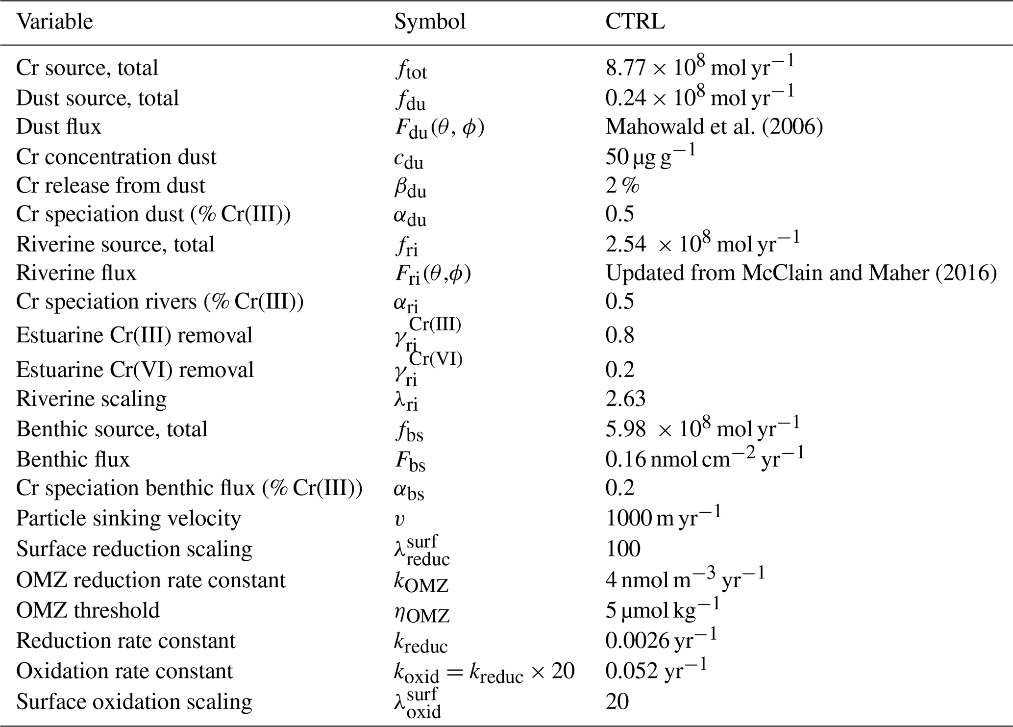
In total, we consider three Cr sources to the ocean: mineral dust, rivers, and a benthic source. The former two are well-constrained vectors of trace metals to the ocean. Yet, during the past years it emerged that for a number of trace metals benthic sources may also play an important role for their respective oceanic inventories (e.g., rare earth elements, Jeandel, 2016; Fe, Mn, and Co, Viera et al., 2019). A benthic Cr source has also been invoked (Cranston, 1983; Jeandel and Minster, 1987), though quantitative estimates of source magnitude are limited by sparse data and are approximate at present (Janssen et al., 2021). Removal of Cr is thought to be controlled by reversible scavenging, which describes the process of adsorption onto sinking particles and subsequent release to the water column during particle remineralization at depth ultimately leading to burial in the underlying sediments.

2.2.1 Sources and sinks

Chromium release from mineral dust, S_du(θ, ϕ), is considered to provide a relatively minor source of Cr to the ocean globally (Goring-Harford et al., 2018; Jeandel and Minster, 1987), yet it may play a relevant role regionally, associated with episodic dust plumes. Due to a lack of constraints, we assume a globally uniform Cr dust concentration (c_du) of 50 ppm, which is at the lower end of measured values for the silicate Earth (Schoenberg et al., 2008), 2 % Cr release in the surface ocean (β_du), and a speciation ratio between Cr(III) and Cr(VI) of 50 % each (α_du). We do not consider further release of Cr from dust in the deeper water column. From these follows

$$\begin{array}{}\text{(2)}& S_{\text{du}}\left(\mathit{\theta },\mathit{\varphi }\right)=F_{\text{du}}\left(\mathit{\theta },\mathit{\varphi }\right)\cdot c_{\text{du}}\cdot {\mathit{\beta }}_{\text{du}}\cdot {\displaystyle \frac{\mathrm{1}}{\mathrm{\Delta }{z}_{\mathrm{1}}}},\end{array}$$

where Δz₁ is the height of the surface ocean layer. Accordingly, the Cr(III) and Cr(VI) dust fluxes are

$$\begin{array}{}\text{(3)}& {\displaystyle }{S}_{\text{du}}^{\text{Cr}\left(\text{III}\right)}\left(\mathit{\theta },\mathit{\varphi }\right)=S_{\text{du}}\left(\mathit{\theta },\mathit{\varphi }\right)\cdot {\mathit{\alpha }}_{\text{du}},\text{(4)}& {\displaystyle }{S}_{\text{du}}^{\text{Cr}\left(\text{VI}\right)}\left(\mathit{\theta },\mathit{\varphi }\right)=S_{\text{du}}\left(\mathit{\theta },\mathit{\varphi }\right)\cdot \left(\mathrm{1}-{\mathit{\alpha }}_{\text{du}}\right).\end{array}$$

The riverine Cr source, S_ri(θ, ϕ), is prescribed based on the database by McClain and Maher (2016) with updated and extended observations from Guinoiseau et al. (2016), Skarbøvik et al. (2015), and Wei et al. (2018), while rivers showing strong anthropogenic contamination were removed (Supplement Sect. S1). Overall, detailed constraints related to the speciation of the riverine sources are incomplete, and we hence assume an initial Cr(III) to Cr(VI) ratio of 1:1. Observations indicate that a fraction of dissolved riverine Cr is removed in estuaries (γ_ri) by flocculation processes (e.g., Campbell and Yeats, 1984; Mayer and Schick, 1981; Shiller and Boyle, 1991). Yet, estimates for Cr(III) and Cr(VI) removal rates vary widely (Goring-Harford et al., 2020; Mayer and Schick, 1981; Morris, 1986), and some studies even indicate an increase in total dissolved Cr with salinity (e.g., Sun et al., 2019). Hence, we adopt a simplified parametrization that is in general agreement with these estimates and the overall chemical behavior of the scavenging-prone Cr(III) to be removed by 80 % and the much more soluble Cr(VI) to be removed only by 20 %. Since our riverine database covers only rivers accounting for a fraction of the global discharge, we uniformly scale all riverine fluxes by a factor (λ_ri) to compensate for the missing data. Arguably, this over represents larger, well-studied rivers and thus skews the distribution of riverine Cr fluxes to the oceans, but such a simplification is consistent with the intermediate complexity of the Bern3D model. The riverine Cr fluxes per unit volume, V(θ, ϕ), thus read

$$\begin{array}{}\text{(5)}& {\displaystyle }\begin{array}{rl}& S_{\text{ri}}^{\text{Cr}\left(\text{III}\right)}\left(\mathit{\theta },\mathit{\varphi }\right)=F_{\text{ri}}\left(\mathit{\theta },\mathit{\varphi }\right)\cdot c_{\text{ri}}\cdot {\mathit{\alpha }}_{\text{ri}}\cdot \left(\mathrm{1}-{\mathit{\gamma }}_{\text{ri}}^{\text{Cr}\left(\text{III}\right)}\right)\\ & \cdot {\mathit{\lambda }}_{\text{ri}}\cdot {\displaystyle \frac{\mathrm{1}}{\text{V}\left(\mathit{\theta },\mathit{\varphi }\right)}},\end{array}\text{(6)}& {\displaystyle }\begin{array}{rl}& S_{\text{ri}}^{\text{Cr}\left(\text{VI}\right)}\left(\mathit{\theta },\mathit{\varphi }\right)=F_{\text{ri}}\left(\mathit{\theta },\mathit{\varphi }\right)\cdot c_{\text{ri}}\cdot \left(\mathrm{1}-{\mathit{\alpha }}_{\text{ri}}\right)\cdot \left(\mathrm{1}-{\mathit{\gamma }}_{\text{ri}}^{\text{Cr}\left(\text{VI}\right)}\right)\\ & \cdot {\mathit{\lambda }}_{\text{ri}}\cdot {\displaystyle \frac{\mathrm{1}}{V\left(\mathit{\theta },\mathit{\varphi }\right)}}.\end{array}\end{array}$$

Finally, the third major source of Cr in the model is a benthic flux, S_bs(θ, ϕ), emanating from all sediment–water interfaces. Pore-water Cr data are limited (Brumsack and Gieskes, 1983; Shaw et al., 1990), and currently, only one open ocean pore-water [Cr] profile exists that quantifies the first-order magnitude of the flux (Janssen et al., 2021). Hence, no inferences on the spatial variability in this source can be made at this point. We therefore apply a globally uniform parametrization for the benthic flux. Based on the pore-water investigations by Janssen et al. (2021), it is suggested that adsorbed Cr(III) is slowly oxidized back to soluble Cr(VI) in the pore water, which accumulates and ultimately escapes from the sediment due to the build up of a concentration gradient between bottom and pore waters. We therefore assume that the majority (80 %) of the benthic Cr flux is in the form of Cr(VI), which leads to

$$\begin{array}{}\text{(7)}& {\displaystyle }{S}_{\text{bs}}^{\text{Cr}\left(\text{III}\right)}\left(\mathit{\theta },\mathit{\varphi },z\right)=F_{\text{bs}}\cdot {\mathit{\alpha }}_{\text{bs}}\cdot {\displaystyle \frac{\mathrm{1}}{\text{V}\left(\mathit{\theta },\mathit{\varphi },z\right)}},\text{(8)}& {\displaystyle }{S}_{\text{bs}}^{\text{Cr}\left(\text{VI}\right)}\left(\mathit{\theta },\mathit{\varphi },z\right)=F_{\text{bs}}\cdot \left(\mathrm{1}-{\mathit{\alpha }}_{\text{bs}}\right)\cdot {\displaystyle \frac{\mathrm{1}}{V\left(\mathit{\theta },\mathit{\varphi },z\right)}},\end{array}$$

where α_bs is the ratio of Cr(III) to Cr(VI) speciation.

The sole sink of Cr considered in the model relates to the removal and export of Cr with sinking particles. The reversible scavenging scheme used in the Bern3D model is described in detail by Rempfer et al. (2011) and follows previous descriptions (Henderson et al., 1999; Marchal et al., 2000). In brief, the scavenging efficiencies of Cr(III) and Cr(VI) to the four different particles types i (CaCO₃, POM, biogenic opal, lithogenics) are described by the particle affinity coefficients $K_{\text{d}}^i$. It is the magnitude of $K_{\text{d}}^i$ that determines the solubility of the different ocean tracers. Removal rates are further shaped by the particle concentration and the particle sinking velocity (v), which is considered globally uniform and constant (1000 m yr⁻¹). Particles reaching the seafloor are fully remineralized, while the associated Cr is removed from the model, ultimately balancing the source terms.

2.2.2 Internal cycling

Reversible scavenging not only prescribes Cr removal at the seafloor but also modulates the redistribution of Cr within the water column. At shallow depths reversible scavenging acts as a net sink, contributing to reduce the dissolved Cr fraction, while it works as a net source at greater depths where adsorbed Cr is released back into solution. The internal Cr cycling is further influenced by redox reactions. A handful of studies investigated redox reactions and pathways in controlled laboratory experiments, aiming to determine reaction rate constants (e.g., Emerson et al., 1979; Pettine et al., 1998, 2008). As a note of caution, these experiments were conducted with substantially higher reactant concentrations than typically observed in the modern ocean, and thus simple extrapolations to mean ocean concentrations may not always be fully valid. We therefore consider these reaction rates only as first-order approximations and further adjust them during model tuning.

Divalent iron, Fe(II), which is produced by photochemical (e.g., Barbeau et al., 2001) and biological processes (e.g., Maldonado and Price, 2001) in surface waters, constitutes the main reductant for Cr (Pettine et al., 1998). In order to reflect these surface-specific processes in the model, Cr reduction is parameterized differently in the surface ocean compared to the deep where photochemical and biologically mediated reactions are strongly attenuated or likely absent. Thus, Cr(VI) reduction is increased in the uppermost grid cells by a factor ${\mathit{\lambda }}_{\text{reduc}}^{\text{surf}}$ compared to the deep ocean, and a dependency on POM export productivity, P_POM(θ,ϕ), relative to its global maximum is introduced. While reaction rates are dependent on the concentrations of the reactants, Fe(II) and other potential reductants are not explicitly implemented in the model. Chromium reduction in the model is thus solely controlled by the Cr(VI) concentration as follows:

$$\begin{array}{}\text{(9)}& \begin{array}{rl}& R_{\text{VI}\to \text{III}}^{\text{surf}}\left(\mathit{\theta },\mathit{\varphi }\right)=k_{\text{reduc}}\cdot {\mathit{\lambda }}_{\text{reduc}}^{\text{surf}}\cdot \left[\text{Cr}\left(\text{VI}\right)\right]\left(\mathit{\theta },\mathit{\varphi }\right)\\ & \cdot {\displaystyle \frac{P_{\text{POM}}\left(\mathit{\theta },\mathit{\varphi }\right)}{P_{\text{POM,MAX}}}},\end{array}\end{array}$$

where k_reduc (yr⁻¹) is the rate constant also used for the tuning, and for the deep ocean it is

$$\begin{array}{}\text{(10)}& R_{\text{VI}\to \text{III}}^{\text{deep}}\left(\mathit{\theta },\mathit{\varphi },z\right)=k_{\text{reduc}}\cdot \left[\text{Cr}\left(\text{VI}\right)\right]\left(\mathit{\theta },\mathit{\varphi },z\right).\end{array}$$

In the ocean interior, Cr reduction is also observed in oxygen minimum zones (OMZs) (e.g., Cranston and Murray, 1978; Huang et al., 2021; Murray, 1983; Rue et al., 1997), although data on reaction and removal rates (k_OMZ) remain very sparse. We include this specific process in the model and prescribe dissolved O₂ concentrations < 5 µmol kg⁻¹ as the threshold (η_OMZ) below which Cr reduction is strongly enhanced in the model (Moos et al., 2020; Nasemann et al., 2020).

$$\begin{array}{}\text{(11)}& R_{\text{VI}\to \text{III}}^{\text{OMZ}}\left(\mathit{\theta },\mathit{\varphi },z\right)=k_{\text{OMZ}}\cdot \left\{\begin{array}{cc}\mathrm{1}& \mathrm{for}\left[{\mathrm{O}}_{\mathrm{2}}\right]\left(\mathit{\theta },\mathit{\varphi },z\right)\le {\mathit{\eta }}_{\text{OMZ}}\\ \mathrm{0}& \mathrm{else}\end{array}\right.\end{array}$$

On the other hand, Cr(III) is slowly oxidized back to Cr(VI) for instance by H₂O₂ (Pettine et al., 2008). Hydrogen peroxide concentrations decrease with depth due to photochemical production, atmospheric deposition to surface waters, and subsequent decomposition (Kieber et al., 2001). We therefore additionally introduce a surface scaling for the oxidation ${\mathit{\lambda }}_{\text{oxid}}^{\text{surf}}$ analogous to Eq. (9).

$$\begin{array}{}\text{(12)}& {\displaystyle }{R}_{\text{III}\to \text{VI}}^{\text{surf}}\left(\mathit{\theta },\mathit{\varphi }\right)=k_{\text{oxid}}\cdot {\mathit{\lambda }}_{\text{oxid}}^{\text{surf}}\cdot \left[\text{Cr}\left(\text{III}\right)\right]\left(\mathit{\theta },\mathit{\varphi }\right)\text{(13)}& {\displaystyle }{R}_{\text{III}\to \text{VI}}^{\text{deep}}\left(\mathit{\theta },\mathit{\varphi },z\right)=k_{\text{oxid}}\cdot \left[\text{Cr}\left(\text{III}\right)\right]\left(\mathit{\theta },\mathit{\varphi },z\right)\end{array}$$

Summing up all external sources into S_tot(θ,ϕ,z) and combining the surface and deep ocean oxidation and reduction equations $R_i^{\text{surf}}$ and $R_i^{\text{deep}}$ into R_i, the conservation equations can be written as

$$\begin{array}{}\text{(14)}& {\displaystyle }\begin{array}{rl}& {\displaystyle \frac{\partial \left[\text{Cr}\left(\text{III}\right)\right]}{\partial t}}=S_{\text{tot}}{\left[\text{Cr}\left(\text{III}\right)\right]}_{\text{d}}+R_{\text{VI}\to \text{III}}+R_{\text{VI}\to \text{III}}^{\text{OMZ}}\\ & -R_{\text{III}\to \text{VI}}-{\displaystyle \frac{\partial \left(v\cdot \left[\text{Cr}{\left(\text{III}\right)}_{\text{p}}\right]\right)}{\partial z}}+\text{T}\left[\text{Cr}\left(\text{III}\right)\right],\end{array}\text{(15)}& {\displaystyle }\begin{array}{rl}& {\displaystyle \frac{\partial \left[\text{Cr}\left(\text{VI}\right)\right]}{\partial t}}=S_{\text{tot}}{\left[\text{Cr}\left(\text{VI}\right)\right]}_{\text{d}}-R_{\text{VI}\to \text{III}}-R_{\text{VI}\to \text{III}}^{\text{OMZ}}\\ & +R_{\text{III}\to \text{VI}}-{\displaystyle \frac{\partial \left(v\cdot \left[\text{Cr}{\left(\text{VI}\right)}_{\text{p}}\right]\right)}{\partial z}}+\text{T}\left[\text{Cr}\left(\text{VI}\right)\right],\end{array}\end{array}$$

where subscripts d and p indicate the dissolved and particulate phases, respectively, and T corresponds to the physical transport and mixing calculated in the model.

2.2.3 Model tuning

To date the marine Cr cycle remains largely under-constrained, and hence a number of model parameters are either unknown or estimated as first-order approximations. We therefore tuned five different parameters, namely the benthic flux F_bs, the oxidation rate constant k_oxi (related to k_reduc by a constant factor of 20, based on laboratory experiments; Elderfield, 1970; Pettine et al., 1998, 2008), the OMZ reduction rate constant k_OMZ, and reference scavenging parameters for Cr(III) and Cr(VI) (Table S1). The ratios of the affinities to the different particles were held constant and are noted in Table S2. The relatively long residence time of Cr in the ocean, estimated to range between 2 and 40 kyr (Campbell and Yeats, 1981; Sirinawin et al., 2000), requires model integration times at least on the same order of magnitude. This makes a systematic exploration of the five-dimensional tuning parameter space challenging. We therefore employ a Latin hypercube sampling approach, which significantly reduces the required number of simulations while maintaining good coverage of the parameter space. In total, we performed 500 tuning simulations each integrated over 40 kyr. This was insufficient for all simulations to reach equilibrium. We individually examined this small subset of simulations which had not yet reached equilibrium after 40 kyr and found unrealistically high Cr concentrations in all of them and therefore did not continue model integration for these runs.

The model performance was evaluated by determining the mean absolute error (MAE) of the modern seawater data and [Cr]_tot of the closest model grid cell (root mean squared errors are noted in Table S3). For this, we compiled seawater measurements from the literature (n=701, Table S2). Seawater Cr concentrations have been determined since the late 1970s with increasing efforts in the past years and the recent integration in the GEOTRACES initiative. Early seawater measurements were often performed using unfiltered samples, which led to possible overestimation of dissolved Cr due to particulate phases (Cranston, 1983). Yet, contamination during sample processing may also pose a potential issue (e.g., see discussion in Nasemann et al., 2020). Therefore, we performed a strict quality control and excluded all data for which such concerns were mentioned in the original publications, were identified in later studies, or exhibited inconsistencies such as unrealistically large scatter within a depth profile (see Sect. S1). Finally, we excluded data from coastal stations that were found to be affected by anthropogenic Cr loading (e.g., Hirata et al., 2000; Shiller and Boyle, 1987) or otherwise controlled by localized processes not represented by the resolution of the model, as well as studies in which quantitative comparisons to the model results are limited by poor analytical precision. The final global coverage of seawater Cr measurements is biased towards the top 1000 m of the water column and the North Atlantic and North Pacific.

2.3 Sensitivity experiments

The Arctic Ocean experiences only limited water mass exchange with the adjacent ocean basins via narrow straits. At the same time, it exhibits a high sediment surface-to-ocean volume ratio. Both these circumstances dramatically increase the impact of a benthic flux on the regional tracer budget. Thus, in order to explore the relationship between the benthic flux and the mean Arctic Cr concentration, we conducted an idealized experiment in which we set the benthic flux of Cr to zero north of 70^∘ N (simulation NoArcticBFlux).

Further, due to data constraints, the model tuning was based solely on total Cr concentrations, yet the internal redox cycling and the resulting distribution between Cr(III) and Cr(VI) are also of crucial importance for the potential applicability of Cr and its isotopes as a paleo-redox proxy. To date, a relatively limited amount of information regarding open ocean Cr speciation is available, yet observations suggest widespread Cr reduction in OMZs below a threshold O₂ concentration (Goring-Harford et al., 2018; Huang et al., 2021; Moos et al., 2020; Rue et al., 1997). In order to explore the consequences of OMZ Cr reduction on the global Cr inventory, we performed a number of idealized sensitivity experiments. As noted in Sect. 2.1, in our standard configuration POM remineralization is prescribed as a globally uniform power-law profile (Martin et al., 1987). Even though total export fluxes are in good agreement with observations using such parametrization (Parekh et al., 2008), the POM remineralization in OMZs is not adequately represented. Recently, Battaglia and Joos (2018) introduced a new formulation in the Bern3D model that assigns POM remineralization to aerobic or anaerobic pathways depending on the dissolved O₂ concentration. Both are defined as power-law profiles yet with different remineralization length scales, yielding reduced remineralization rates under anaerobic conditions (see Battaglia Battaglia and Joos, 2018 for details). We therefore performed a set of sensitivity experiments in which we replaced the globally uniform POM remineralization with the improved parametrization introduced by Battaglia and Joos (2018) (simulation OMZrem).

In a third experiment, we investigated the impact of a substantially stronger Cr reduction rate in OMZs as suggested by field observations (Huang et al., 2021; Moos et al., 2020; Rue et al., 1997). For this simulation we increased the OMZ reduction rate from 4 nmol m⁻³ yr⁻¹ in the control run to 20 nmol m⁻³ yr⁻¹ while also using the improved two-pathway POM remineralization of Battaglia and Joos (2018) (simulation OMZrem20). Finally, we performed an experiment with an even higher reduction rate of 30 nmol m⁻³ yr⁻¹ (OMZrem30). All these experiments were branched off from the fully equilibrated control (CTRL) run under pre-industrial boundary conditions and are summarized in Table 2.

Table 2 Different model simulations. Parameters not listed here were kept as in the control run (see Table 1). The mean absolute error (MAE) was determined by comparing seawater observations to the model output at the closest grid cell.

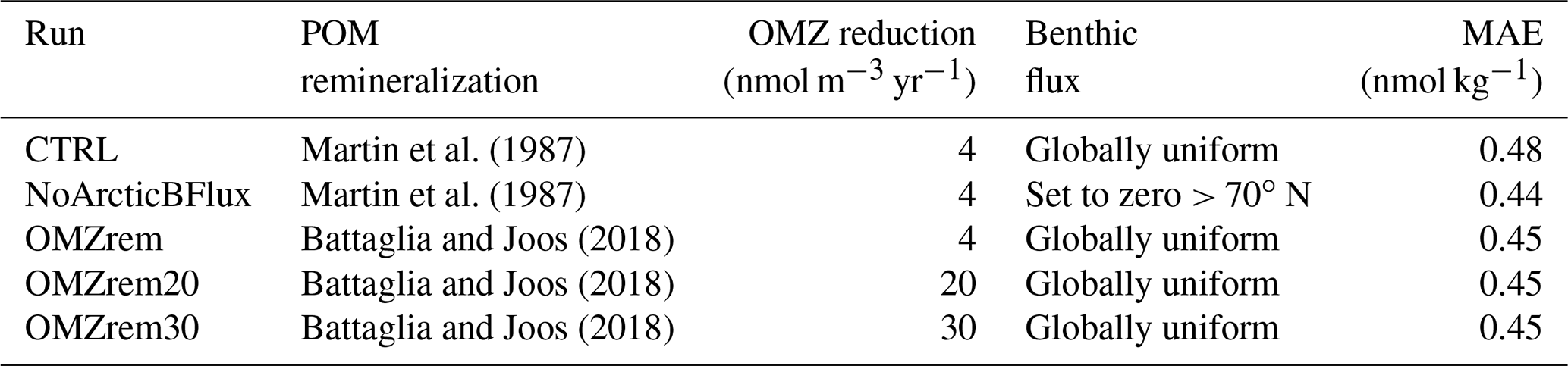
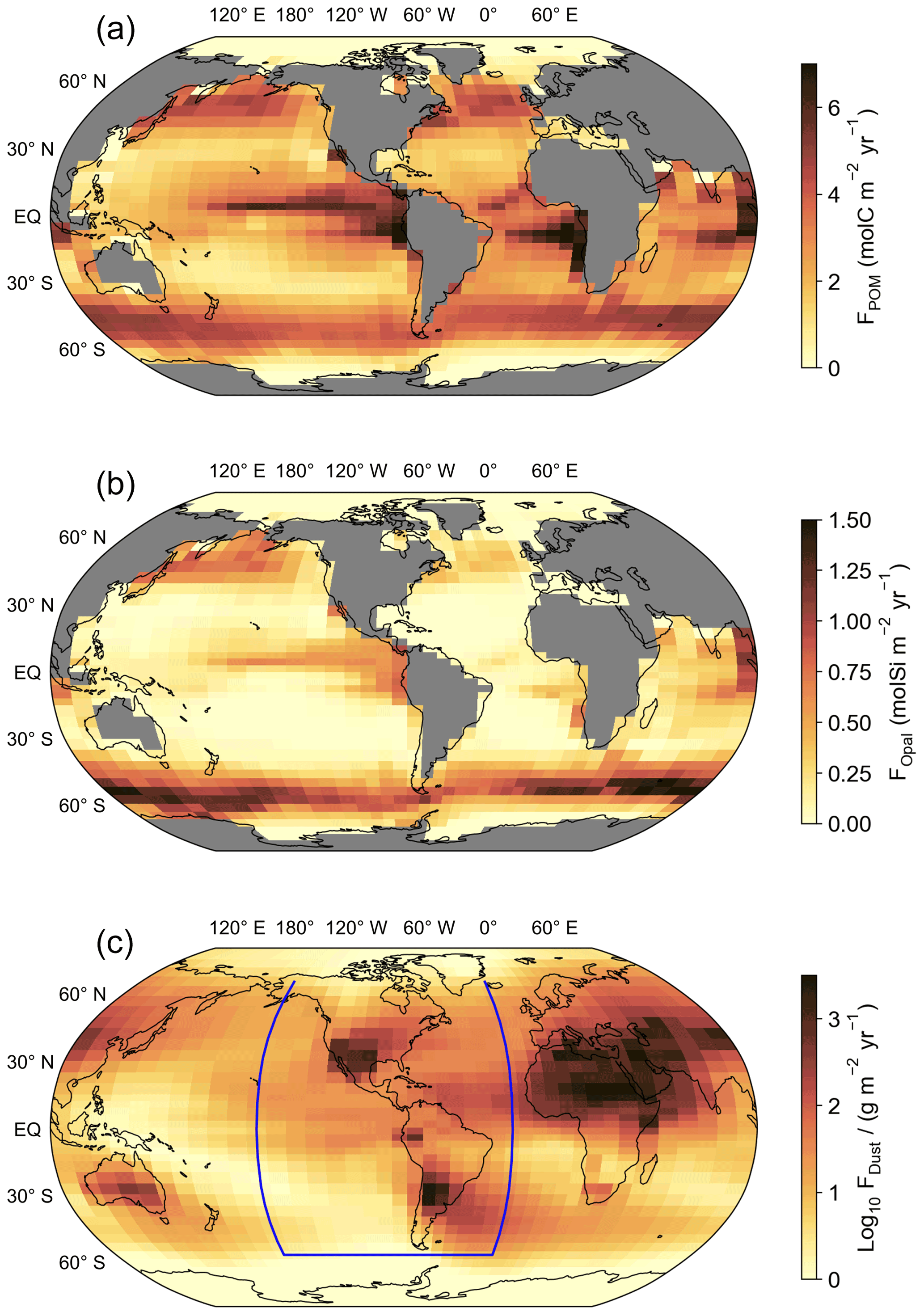
Figure 1 (a) Export fluxes of particulate organic matter (POM) and (b) biogenic opal calculated in the biogeochemical model from prognostic equations (Parekh et al., 2008). The distribution of calcium carbonate (CaCO₃) production is the same as for POM but scaled by the Redfield ratio and a Ca to P ratio of 0.3 in calcifiers. (c) Log10 of the global dust flux estimated by Mahowald et al. (2006). The blue line indicates the transect for the section plots of Fig. 5.

3 Results

3.1 Constraints on benthic flux and residence time of Cr

A wide array of estimates for the oceanic residence time of Cr exists (defined as the total inventory divided by the sum of all source fluxes) ranging from 2 to 40 kyr (McClain and Maher, 2016; Sirinawin et al., 2000; Wei et al., 2018). In our parametrization, the mean ocean residence time of Cr is strongly influenced by the magnitude of the newly introduced benthic flux representing the largest source in nearly all runs of the 500-member tuning ensemble. From this tuning ensemble, we already obtain first constraints on the magnitude of the benthic flux, as well as the mean ocean residence time of Cr, as both converge towards low MAEs (Fig. 2). In the ensemble, the best model–data agreement is achieved with benthic fluxes in the range of 0.1 to 0.2 nmol cm⁻² yr⁻¹, substantially lower than the estimate from the Tasman Basin that suggested a benthic flux of ∼ 3.2 nmol cm⁻² yr⁻¹ (Janssen et al., 2021). Overall, simulations with large benthic fluxes on the order of 1 nmol cm⁻² yr⁻¹ produce either Cr concentrations that are too high or unrealistically strong vertical gradients (due to the large bottom source in combination with strong particle scavenging that is required under such conditions to balance the large benthic source flux). The clear trend in the model–data misfit of the ensemble (Fig. 2a) indicates that reduced benthic fluxes are a fairly robust result with the parametrization applied (i.e., globally uniform flux). Thus, we suspect that the benthic flux observed in the Tasman Basin may not be fully representative of the global ocean seafloor. However, missing processes in the internal cycling of the model that could be responsible for the mismatch cannot be fully excluded at this point. Further, we note that we cannot distinguish whether the benthic Cr is of authigenic or lithogenic origin in the model since we do not employ a sediment module for the calculation of the pore-water chemistry. It is thus possible that the benthic Cr is to some extent recycled primary Cr from dust and rivers and not “new” Cr that is added to the marine reservoir from the sediments. In that case, the ocean residence time of Cr would increase proportionally to the fraction of recycled Cr of the benthic source. As benthic sources account for approximately two-thirds of the total Cr source in our model (Table 1), this would yield a maximal increase of approximately a factor of 3 for our calculated residence times.

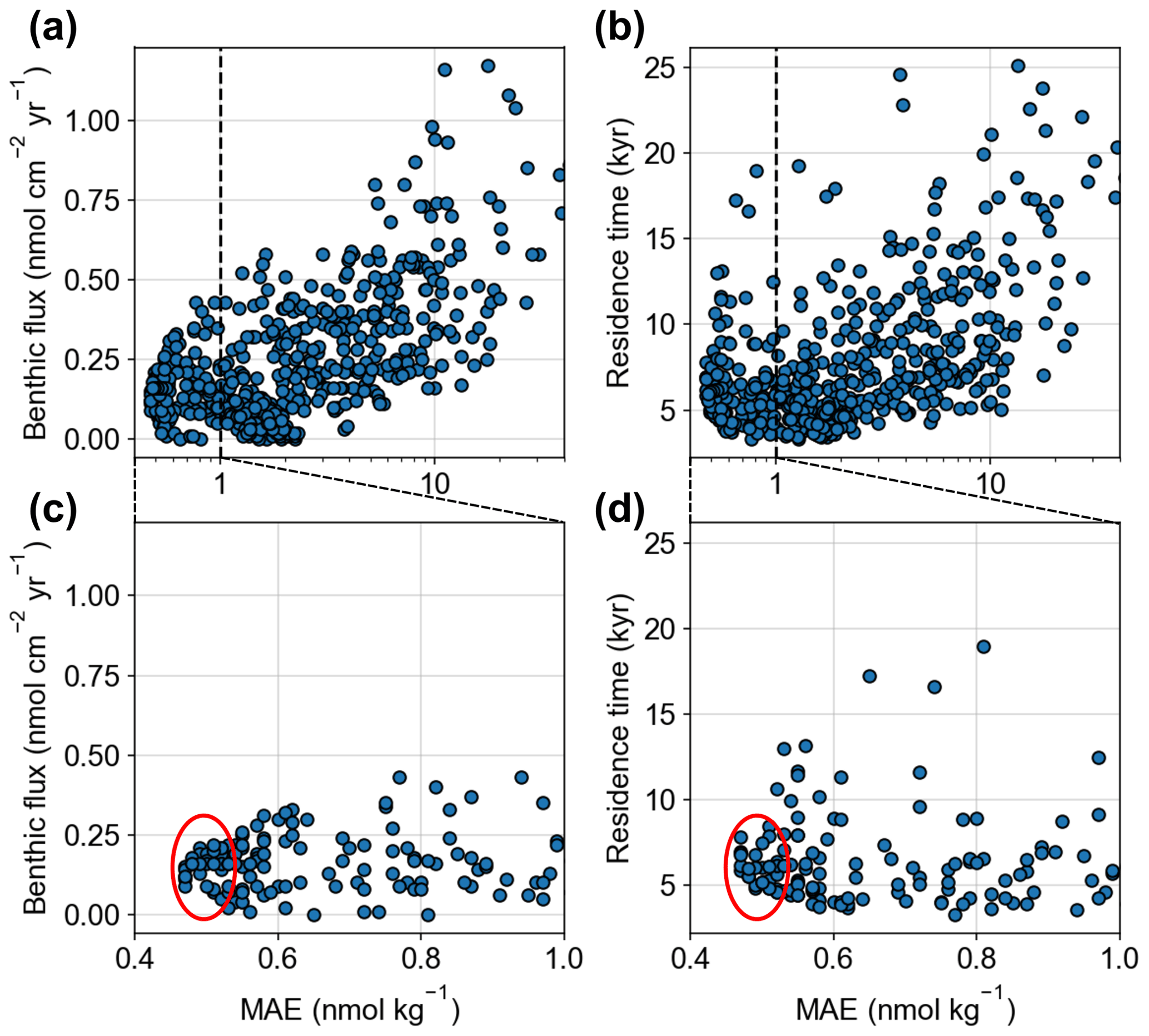
Figure 2 (a, c) Model performance of the tuning ensemble (calculated with the cost function of the mean absolute error, MAE – the smaller the better) dependent on the benthic flux and (b, d) the diagnosed mean residence time of dissolved Cr. Note the logarithmic x axes in (a, b). (c, d) are zoom-ins of (a) and (b) and with linear x axes. Red ellipses indicate the simulations that best fit the observational data.

The trend in the residence time versus model–data mismatch is somewhat less distinct than that for the benthic flux (Fig. 2b), but it still clearly converges towards the lower end of previous estimates. The simulations that best fit the observational data all exhibit Cr residence times between 5 and 8 kyr (Fig. 2d). These relatively short residence times, compared to previous upper-limit estimates, are to some degree expected considering that benthic fluxes were either neglected or assumed to be fairly small in previous studies (e.g., Reinhard et al., 2013) but are in contrast to the dominant Cr source in our model simulations. Yet, previous lower-limit estimates also did not include significant benthic sources but instead included anthropogenically contaminated rivers with exceedingly high Cr concentrations (e.g., the Panuco River; McClain and Maher, 2016), which are not considered here.

3.2 Model–data comparison of the control run

The tuning ensemble member that best fits the observational data of dissolved Cr concentrations (defined as the control run) yields an MAE of 0.48 nmol kg⁻¹. A few other simulations performed virtually as well as the control run, all of which exhibited similar values for the benthic flux and the scavenging factors. However, the parameters that describe the internal cycling (i.e., oxidation rate and OMZ reduction rate) exhibit a wider spread among these simulations. This is related to the fact that our tuning target was solely the total Cr concentration, and we did not consider the individual oxidation states in assessing model performance due to insufficient data coverage to achieve statistical significance. The parameters of the control run are listed in Table 1.

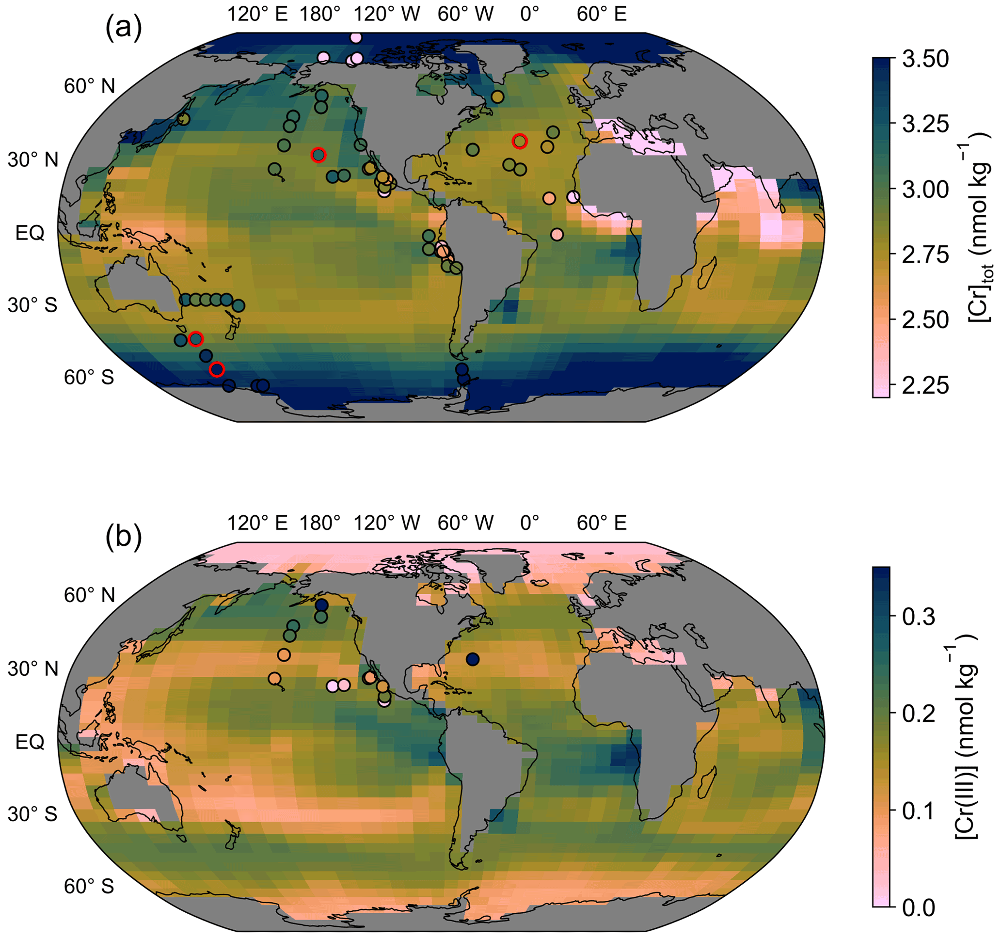
Figure 3 (a) Surface ocean total dissolved Cr concentration simulated in the control run. Filled circles mark surface seawater observations (top 40 m, equivalent to the height of the uppermost grid cell) with colors on the same scale as background model data. Circles with red edges are stations depicted in Fig. 6. (b) Same as (a) but for Cr(III) concentrations.

In the control run, the total flux of Cr entering the ocean amounts to 8.77 × 10⁸ mol yr⁻¹ with the smallest contribution from dust (∼ 3 %), followed by the riverine source (∼ 29 %), and by far the largest contribution from the benthic flux (∼ 68 %) (Table 1). Even though the global benthic flux of 0.16 nmol cm⁻² yr⁻¹ in the control run is much smaller than the first local estimate (Janssen et al., 2021), it still dwarfs the combined contributions from dust and rivers. In contrast, assuming both dust and river sources as in the control run but a benthic flux comparable to the first local estimate (∼ 3 nmol cm⁻² yr⁻¹) would yield a benthic flux contribution of ∼ 98 % and be about 50 times larger than the riverine source. As previously noted by Janssen et al. (2021), it thus appears that this first observational estimate for the benthic flux from the Tasman Basin may not be fully representative of the global ocean, and further research regarding the impacts of sediment composition, porosity, and bottom and pore-water chemistry is required to better constrain this presumably significant Cr source to the ocean.

3.2.1 Surface ocean

The surface ocean [Cr]_tot simulated in the control run reveals a distinct meridional gradient with the highest values of around 3.5 nmol kg⁻¹ in the high latitudes decreasing equatorwards (Fig. 3). The lowest surface [Cr]_tot is simulated in the high-productivity regions off the coast of East Africa and the equatorial Indian Ocean, as well as in the Mediterranean Sea. However, caution should be placed on the interpretation of the simulated Cr concentrations in semi-enclosed basins such as the Mediterranean Sea, which are poorly represented by the coarse spatial resolution of the model. Overall, Cr is more strongly reduced in upwelling regions, which together with the high particle concentrations associated with high primary productivity (Fig. 1) promotes efficient scavenging. Surface Cr concentrations are further impacted by large river systems with high dissolved Cr concentrations such as the Congo River, the Yangtze, or the Ganges–Brahmaputra, which produce elevated concentrations at their river mouths.

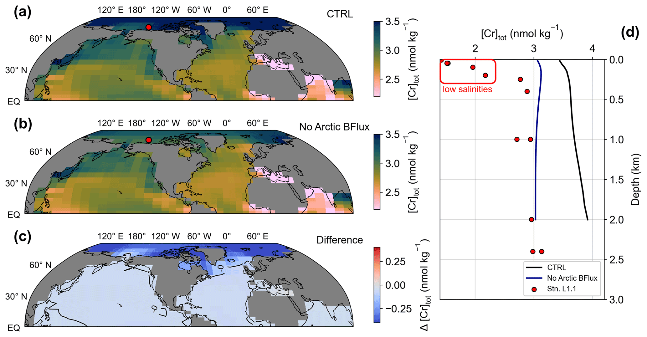
Figure 4 (a–c) Surface total Cr concentrations for simulations CTRL and NoArcticBFlux, as well as the difference between both. The red circle marks the location of station L1.1 of Scheiderich et al. (2015) depicted in (d). (d) [Cr]_tot depth transect from the Arctic. Lines represent model output of simulations CTRL (black) and NoArcticBFlux (blue) of the grid cells closest to station L1.1 (red circles).

The comparison of the control run to observational Cr data in the uppermost 40 m (height of the surface grid cell) shows good agreement overall. For instance, the strong meridional gradient in the Southern Ocean described above is also represented in a meridional transect from Antarctica to southern Australia (Rickli et al., 2019). In contrast, open ocean low- to mid-latitude surface Cr concentrations are slightly underestimated by the model compared to seawater data. The largest model–data discrepancy is observed in the Arctic Ocean where recent GEOTRACES data reveal remarkably low surface Cr concentrations (Scheiderich et al., 2015), while simulated Cr concentrations are substantially higher (Figs. 4d; S1).

These observed low surface Cr concentrations are accompanied by low salinities indicating the influence of meltwater (Scheiderich et al., 2015). The exceptionally low trace metal concentrations in meltwater (due to the salt rejection during formation) may thus be responsible for the Arctic model–data discrepancy. Additionally, in the Bern3D model primary productivity is virtually absent in the Arctic mostly because the summer blooms restricted to coastal environments and near the sea-ice edge cannot be resolved in the model. Further, enhanced Cr reduction by Fe(II) that is released from the organic-rich Arctic shelf sediments is not explicitly implemented here. Thus, Arctic Cr removal by particle scavenging remains extremely limited in the model. In combination with the sluggish exchange with the other ocean basins and the benthic flux constantly adding Cr, this produces elevated Arctic Cr concentrations in the model. We therefore attribute this inadequacy in simulating Arctic Cr to the simplifications in our description of the Cr cycle (e.g., the global uniform benthic flux, which may be substantially smaller in the Arctic) and the relatively coarse resolution of the model. We test the former attribution in a sensitivity experiment (simulation NoArcticBFlux) by setting the benthic flux to zero north of 70^∘ N. Indeed, Arctic surface Cr concentrations are up to 0.5 nmol kg⁻¹ lower in simulation NoArcticBFlux compared to CRTL (Fig. 4). This suggests that the benthic flux has significant impact even on surface concentrations in the semi-enclosed Arctic basin.

The surface distribution of Cr(III) (Fig. 3b) somewhat represents that of the POM export productivity (Fig. 1). This is related to our choice of parametrization that scales the surface Cr reduction rate with the POM export (see Sect. 2.2). However, differences are apparent as spatial variations are smaller for Cr(III) due to high removal rates by particle scavenging in regions with high Cr reduction rates (i.e., high-productivity regions).

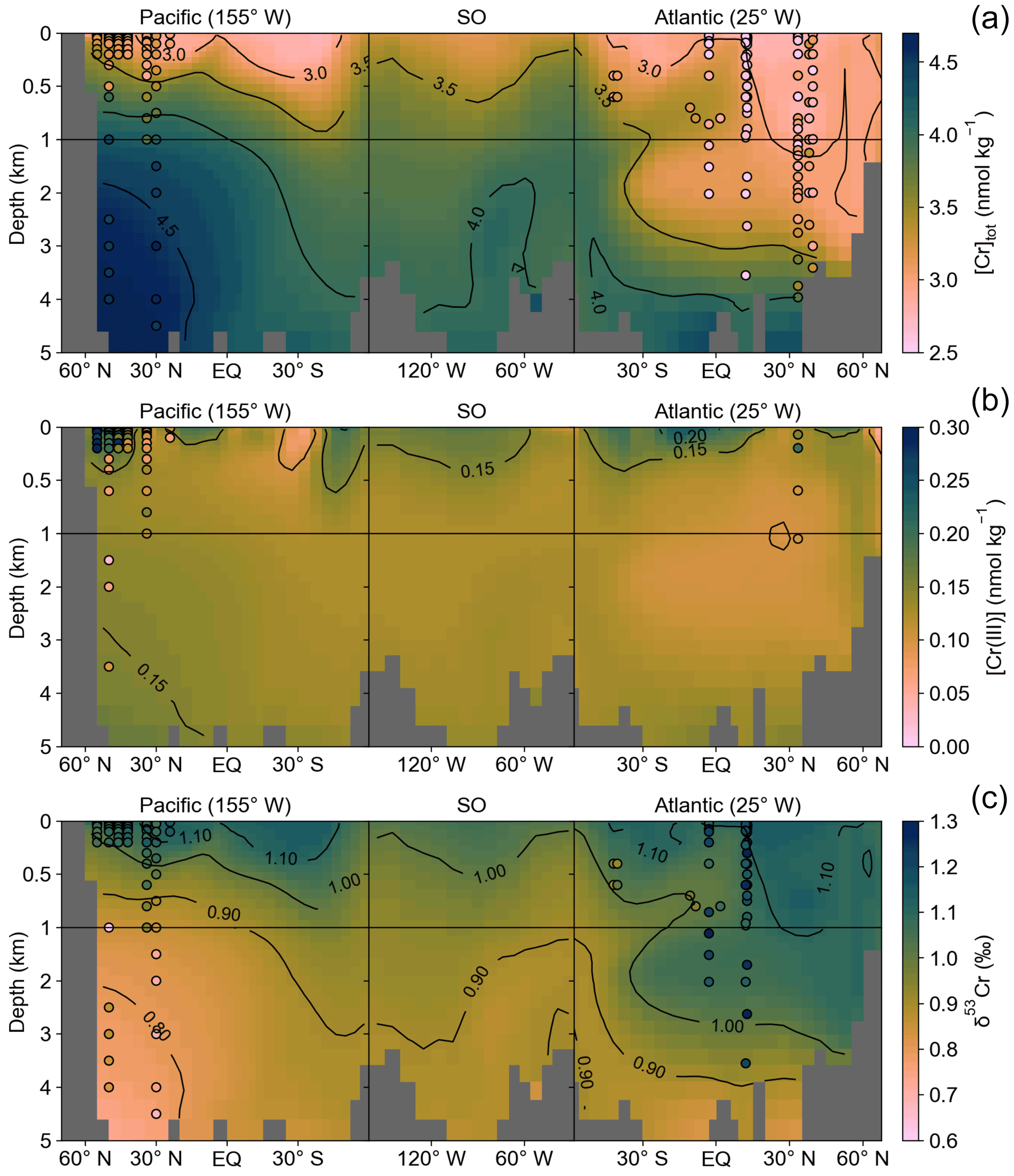
Figure 5 (a) Total dissolved Cr concentrations along the transect marked in Fig. 1 from the North Pacific via the Southern Ocean (SO) to the North Atlantic. Filled circles are seawater observations on the same color scale as the model data. (b) Dissolved Cr(III) distribution along the same transect as in (a). (c) Calculated δ⁵³Cr distribution based on the global ocean array assuming δ⁵³Cr = −0.70 ⋅ ln([Cr]_tot) + 1.86 (Janssen et al., 2021) compared to observational isotope ratio data. Only observational seawater data close to the transect (±15^∘) are shown. Note the different y scales for the top 1 km.

Seawater Cr(III) measurements are comparatively sparse, and reported data are partly inconsistent presumably due to its high reactivity complicating sample processing, standardization, and intercalibration, as well as the lack of sample filtering in some studies (e.g., Connelly et al., 2006). Thus, a model–data assessment is premature at the current stage. Nevertheless, the North Pacific meridional gradient from the high-productivity region off the coast of Alaska to the oligotrophic subtropical gyre by Janssen et al. (2020) is fairly well-represented in the control run. Yet, we reiterate that the model tuning was not targeted at optimizing the Cr(III) distribution, and a better representation of trivalent Cr in the model could most likely be achieved with a better coverage of observational data and an improved understanding of the Cr redox behavior in the ocean.

3.2.2 Deep ocean

The distribution of simulated deep ocean total Cr concentrations is characterized by two pronounced and globally consistent features (Figs. 5, 6). First is an increase in Cr concentrations with depth that is smallest in the Southern Ocean and northern North Atlantic (Δ[Cr]_tot ≈1 nmol kg⁻¹; top-to-bottom difference) and largest in the North Pacific (Δ[Cr]_tot>2 nmol kg⁻¹). The only exception to this feature appears in the South Atlantic where Antarctic Intermediate Water with fairly high total Cr concentrations overlays North Atlantic Deep Water (NADW), characterized by generally lower dissolved Cr. The second feature relates to the accumulation of Cr as water masses age, with the lowest concentrations in waters dominated by newly formed NADW ([Cr]_tot≈3 nmol kg⁻¹) and gradually increasing towards the North Pacific where deep waters exhibit total Cr concentrations > 4.5 nmol kg⁻¹ (Fig. S3). Both these characteristics arise from the reversible scavenging scheme resulting in the net downward transport of Cr in combination with the benthic flux gradually increasing bottom water Cr concentrations.

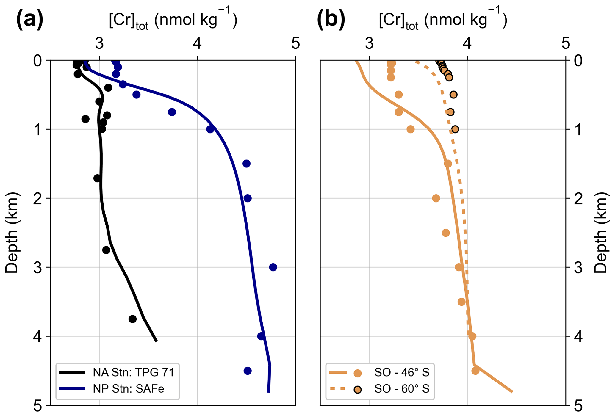
Figure 6 Comparisons between measured total Cr concentrations of four seawater stations (circles) and simulated values of the control run at the closest model grid cells (lines). North Atlantic station TPG 71 (Jeandel and Minster, 1987), North Pacific station SAFe (Moos and Boyle, 2019), and Southern Ocean stations at 46^∘ S (composite of IN2018V04 – Stn. PS2, Janssen et al., 2021, and ACE Leg2 – Stn. 8, Rickli et al., 2019) and 60^∘ S (ACE Leg2 – Stn. 10, Rickli et al., 2019).

On a global scale, observational [Cr]_tot data show very similar trends as simulated by the Bern3D model. Differences between the model and observations are mainly found in the Atlantic basin, where the model generally overestimates total Cr concentrations (while surface concentrations are underestimated as discussed above). Part of the Atlantic model–data mismatch might be attributed to the model simulating NADW that is too shallow due to deep water formation taking place too far south (Müller et al., 2006). Thus, the extent of the low Cr concentration NADW endmember is underestimated in the model. Further, as mentioned above, simulated Arctic [Cr]_tot is far too high compared to observations. This regional model shortcoming is to some extent also propagated into the Atlantic as Arctic water export through the Fram Strait contributes to the formation of NADW. In simulation NoArcticBFlux, in which the benthic flux is set to zero at latitudes > 70^∘ N, Arctic deep ocean Cr concentrations are up to 1 nmol kg⁻¹ lower compared to CTRL (Fig. 4d), which indeed not only improves the model–data agreement in the Arctic but also in the North Atlantic (Table 2). Thus, simulated Atlantic Cr concentrations could be improved, for instance, by a revised representation of North Atlantic deep water formation and a better understanding of regional differences in the benthic flux.

Figure 7 Eastern equatorial Pacific (7.5^∘ N, 90^∘ W) (a) oxygen concentration for CTRL (i.e., globally uniform POM remineralization) and the O₂-dependent remineralization as described by Battaglia et al. (2018) used for the sensitivity experiments. (b) Total Cr and Cr(III) concentrations for CTRL and simulation OMZrem. (c) Same as (b) but for simulations OMZrem20 and OMZrem30.

In a simplified approach we also converted the simulated total Cr concentration to stable isotopic ratios based on the global oceanic array that exhibits a linear relationship between δ⁵³Cr and ln([Cr]_tot) (Fig. 5). Here we use δ⁵³Cr = −0.70 ⋅ ln([Cr]_tot) + 1.86 based on Janssen et al. (2021). This also allows us to compare the model results to seawater isotopic ratios that are obtained independently of the Cr concentrations. Overall, the model–data agreement for the isotopic ratios is comparable to [Cr]_tot, indicating that deviations from the global array due to different fractionation processes, as suggested for instance for OMZs (Moos et al., 2020; Nasemann et al., 2020), have limited impact in the open ocean. The Cr model implementation employed here thus holds the promise of also being applicable to investigations of sedimentary Cr stable isotopic data.

In contrast to the fairly variable surface Cr(III) concentrations, its distribution below a water depth of 500 m exhibits remarkable homogeneous values between 0.10 and 0.15 nmol kg⁻¹ throughout most of the well-oxygenated global deep ocean (Fig. 5). Yet, reliable seawater data of open ocean [Cr(III)] are too sparse for a reasonable global-scale model–data comparison, and hence these model results should be taken cautiously.

Table 3 OMZ volumes and sediment area below OMZs, as well as fraction of total Cr burial flux below OMZs. See Table 2 for more specific information on the experiments.

3.3 Improving the representation of Cr reduction in OMZs

Oxygen minimum zones are thought to represent important environments where Cr is removed from the ocean and deposited in the underlying sediments (Moos et al., 2020; Rue et al., 1997) as they promote the reduction of soluble Cr(VI) to scavenging-prone Cr(III). In the model, about one-fourth of the entire Cr removal (calculated from the particulate concentrations of the bottommost grid cells) takes place at the sediments below OMZs (representing an area of 7.37 % of the seafloor; Table 3). Yet, the simulated Cr(III) concentrations of ∼ 0.15 nmol kg⁻¹ are partly in disagreement with observed Cr(III) concentrations in OMZs that can even exceed 1 nmol kg⁻¹ (Huang et al., 2021; Moos et al., 2020; Rue et al., 1997). We consider this to be the result of the model tuning not taking into account the spatial distribution of Cr(III) due to the insufficient data coverage. Generally, modeled Cr(III) concentrations are only slightly elevated in OMZs (Fig. 7b) in contrast to observations that suggest strong reduction rates and subsequent removal of Cr (e.g., Rue et al., 1997).

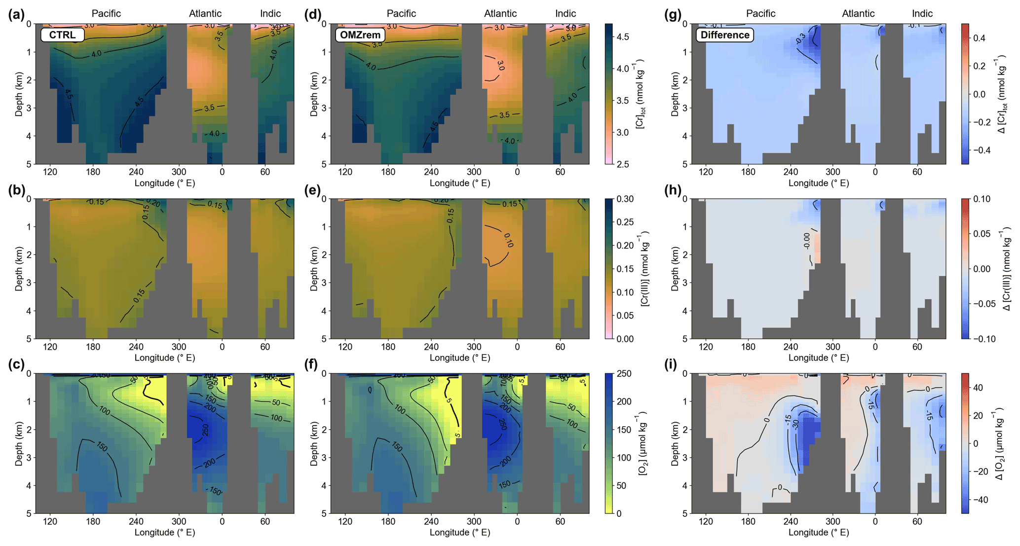
Figure 8 Total Cr (a, d, g), Cr(III) (b, e, h), and O₂ concentrations (c, f, i) along an east–west section at the Equator for the control run (a–c), simulation OMZrem (d–f), and the difference between both (OMZrem minus CTRL) (g–i).

In a first sensitivity experiment (OMZrem) we therefore replaced the globally uniform POM remineralization profile with the O₂-dependent parametrization introduced by Battaglia and Joos (2018) (see Sect. 2.3). This reduces the horizontal expansion of OMZs in the model but at the same time increases their vertical extent (see Fig. 7a). Consequently, the difference in ocean volume where [O₂] < 5 µmol kg⁻¹ is relatively moderate with a decrease from 0.93 % in CTRL to 0.75 % of the total volume with the O₂-dependent remineralization (Fig. 8). However, this is still an overestimation of the modern expansion of OMZs by a factor of about 5 (see Bianchi et al., 2012). This is a persistent issue with Earth system models of various complexity and is mostly related to insufficient spatial resolution to adequately represent these highly dynamic regions even with considerably better spatially resolved models (Cocco et al., 2013).

The greater vertical extent and the strongly attenuated particle remineralization in the OMZs associated with the O₂-dependent parametrization has a profound impact on the vertical [Cr(III)] and [Cr]_tot profiles (illustrated for the eastern equatorial Pacific OMZ in Fig. 7b). In the upper part of the OMZ, Cr(III) concentrations are lower compared to CTRL due to the higher particle concentrations enhancing the scavenging efficiency. In contrast, in the lower part (below 1 km) the effect of the deepened OMZ promoting Cr reduction (local Cr(III) source) dominates over the elevated particle concentrations associated with the vertical expansion (local Cr(III) sink). Both the elevated particle concentration in general and the greater vertical extent of the OMZ increasing Cr reduction (integrated over the entire water column) lead to a decrease in total Cr concentration throughout the water column, yet this effect is most pronounced in the depth range of the OMZ.

Nevertheless, Cr(III) concentrations also remain lower in simulation OMZrem than observations of OMZs indicate (of up to 1 nmol kg⁻¹; Huang et al., 2021). We therefore performed two additional sensitivity experiments with substantially increased OMZ reduction rates of 20 and 30 nmol m⁻³ yr⁻¹ (simulations OMZrem20, OMZrem30, respectively) (compared to 4 nmol m⁻³ yr⁻¹ in CTRL), including the parametrization of O₂-dependent remineralization (Fig. 7c). For both these simulations, Cr(III) concentrations are strongly elevated in OMZs, for instance, peaking at 0.33 and 0.44 nmol kg⁻¹ in the core of the eastern equatorial Pacific OMZ for OMZrem20 and OMZrem30, respectively, compared to a maximum of ∼ 0.20 nmol kg⁻¹ in CTRL. At the same time, the effect of increased OMZ Cr reduction on [Cr]_tot within OMZs is relatively small with a minor decrease in concentrations in the top 1 km and only slightly higher concentrations below. This redistribution in the water column is a direct consequence of the higher Cr(III) concentrations enhancing Cr downward transport and ultimately also removal. Globally this results in 7 % and 12 % more Cr removal below OMZs for simulations OMZrem20 and OMZrem30, respectively, compared to OMZrem (Table 3). As such, the higher OMZ reduction rates, together with the O₂-dependent remineralization, do indeed provide an improved representation of OMZ Cr concentration characteristics (Cr(III) and Cr_tot) consistent with observations (see Moos et al., 2020; Rue et al., 1997). However, it is worthy of note that observations indicate that the Cr(III) maximum in OMZ depth profiles is shifted toward shallower depths (Huang et al., 2021; Rue et al., 1997) and not in the middle or bottom of the OMZ as simulated here. Thus, additional processes such as organic complexation, which stabilizes Cr(III), or elevated Cr reduction at shallow depths might be at play in OMZs that are not explicitly implemented here.

4 Discussion and conclusions

4.1 Global- and regional-scale performance

This study describes the first implementation of the modern marine Cr cycle and more specifically of the two oxidation states, Cr(III) and Cr(VI), into an EMIC. We implemented three Cr sources, namely an aeolian, a riverine, and a benthic flux, that are balanced by the removal associated with reversible scavenging transferring particulate Cr to the sediment. The comparison of our 500-member tuning ensemble to a comprehensive and quality-controlled seawater database provides a best estimate for the mean ocean Cr residence time between 5 and 8 kyr, which is at the lower end of previous first-order approximations (Campbell and Yeats, 1984; Reinhard et al., 2013; Wang et al., 2020). At the same time, we find that the best model–data agreement is achieved with benthic fluxes in the order of 0.1 to 0.2 nmol cm⁻² yr⁻¹, substantially lower than the first local estimates (Janssen et al., 2021). Nevertheless, a benthic flux of such magnitude is substantially larger than the aeolian and riverine source fluxes (for the control run: 68 % benthic, 29 % riverine, and 3 % aeolian).

Overall, the control run simulates the vertical, meridional, and inter-basin [Cr]_tot gradients in good agreement with observational data. Thus, total Cr concentrations increase with depth, as well as with water mass age, which leads to [Cr]_tot > 4.5 nmol kg⁻¹ in the deep North Pacific. Similarly, the vertical gradient increases from Δ[Cr]_tot≈1 nmol kg⁻¹ in the North Atlantic to Δ[Cr]_tot>2.5 nmol kg⁻¹ in the North Pacific. The only major model–data mismatch is observed in the Arctic Ocean basin where simulated concentrations are far too high compared to observations. We attribute this to the poor spatial representation due to the coarse model resolution and to the simplified benthic flux parametrization causing it to have an impact that is too large on this semi-enclosed basin with a large sediment surface area compared to its volume.

In contrast, the poor spatial data coverage of Cr(III) observations precludes not only its incorporation in the tuning metric but also a robust model–data assessment that can only be improved by more seawater measurements. The only exception are OMZs that are fairly well-studied with respect to Cr reduction and hence Cr(III) concentrations (e.g., Huang et al., 2021; Moos et al., 2020; Murray et al., 1983; Rue et al., 1997). Yet, as a consequence of not including Cr(III) in the tuning metric, its representation in OMZs is somewhat deficient. We therefore performed three sensitivity experiments to improve simulated Cr(III) concentrations in these highly reducing regions. By introducing an O₂-dependent parametrization of POM remineralization and a strongly increased OMZ reduction rate, we are able to simulate high Cr(III) concentrations and elevated Cr_tot removal in OMZs that are in much improved agreement with observational data.

4.2 Limitations in simulating the marine Cr cycle

The fairly long mean ocean residence time of Cr puts serious constraints on its implementation in Earth system models. In order to obtain an equilibrated state of the marine Cr cycle, model integrations of several tens of thousands of years are required. This can currently only be achieved with highly computationally efficient, coarse-resolution, intermediate complexity models such as Bern3D. At the same time this limits the representation of the Cr cycle as small-scale processes, for instance at coastal regions, can inherently only be approximated in these models. Furthermore, because of the scarcity of data, processes such as redox reactions, particle scavenging, and sedimentary release of Cr remain critically under-constrained to date, which contributes to substantial uncertainty in the understanding of the marine Cr cycle and thus also impedes its robust implementation in models. As a consequence, only large-scale features of the Cr distributions presented here can be considered as robust. Future improvements in the understanding of, for example, the spatial variability in the benthic flux or the Cr behavior in OMZs, might however bolster our ability to also simulate regional variations in better agreement with observations.

One such more local, yet important, model–data discrepancy relates to the simulated surface depletion of [Cr]_tot that is most pronounced above OMZs but not observed to the same extent in existing seawater profiles (see Figs. 6 and 7; Goring-Harford et al., 2018; Moos et al., 2020; Nasemann et al., 2020). The reversible scavenging scheme linearly scales with the particle concentration. From this follows that Cr removal is strongest in the surface ocean where no remineralization takes place in the model (euphotic zone) and in high-productivity regions that are also responsible for OMZs. One possible explanation to account for the high particle concentrations in these regions not leading to strong surface Cr depletions in the real ocean could relate to complexation with organic ligands. Complexation has been found to be an important process increasing the solubility of a number of trace metals such as rare earth elements (Byrne and Kim, 1990), Cu, Zn, Cd, and most notably Fe (Bruland and Lohan, 2003). Similarly, investigations showed that Cr(III) readily binds with organic ligands (Saad et al., 2017), in contrast to Cr(VI), which seems to be far less affected by complexation (Richard and Bourg, 1991). The dominance of Cr(VI) in oxygenated water therefore indicates that this process is unable to fully explain the simulated surface Cr depletion. Instead, we speculate that internal recycling processes in the mixed layer, not considered in our reversible scavenging parametrization, might be responsible for the observed relatively stable Cr concentrations in the uppermost water column. This could also explain the depleted surface concentrations of other geochemical tracers implemented in the Bern3D model that also make use of the same reversible scavenging formulation (Nd: Pöppelmeier et al., 2020; Pa: Rempfer et al., 2017).

4.3 Future model applications

Despite the uncertainties persisting in the understanding of key processes of the marine Cr cycle, the two main oxidation states of Cr were successfully implemented in the coarse-resolution Bern3D model. This thus provides us with a powerful tool to investigate the biogeochemical cycle of Cr and its isotopes and their tight interconnection with past oceanic and atmospheric oxygenation and biological productivity.

One main focus of future Cr modeling may encompass exploring the impact of expanded OMZs on Cr removal rates. For such endeavors it may be valuable to further improve the parametrization of OMZ-related processes, which should be guided by, for example, new observations of the microbial influence on Cr reduction, as recently suggested by Huang et al. (2021). Furthermore, the Bern3D model is also well-suited for simulations over glacial–interglacial cycles that involve drastic changes not only of the biogeochemistry but also of the ocean circulation and their complex feedbacks.

Finally, past changes in the stable isotopic ratios associated with the fractionation during redox transformations may also be successfully extracted from ocean sediments in the future, which would allow for (semi-)direct comparisons to the Bern3D model.