Using satellite data to identify the methane emission controls of South Sudan's wetlands

The TROPOspheric Monitoring Instrument (TROPOMI) provides observations of atmospheric methane (CH₄) at an unprecedented combination of high spatial resolution and daily global coverage. Hu et al. (2018) reported unexpectedly large methane enhancements over South Sudan in these observations. Here we assess methane emissions from the wetlands of South Sudan using 2 years (December 2017–November 2019) of TROPOMI total column methane observations. We estimate annual wetland emissions of 7.4 ± 3.2 Tg yr⁻¹, which agrees with the multiyear GOSAT inversions of Lunt et al. (2019) but is an order of magnitude larger than estimates from wetland process models. This disagreement may be explained by the underestimation (by up to 4 times) of inundation extent by the hydrological schemes used in those models. We investigate the seasonal cycle of the emissions and find the lowest emissions during the June–August season when the process models show the largest emissions. Using satellite-altimetry-based river water height measurements, we infer that this seasonal mismatch is likely due to a seasonal mismatch in inundation extent. In models, inundation extent is controlled by regional precipitation scaled to static wetland extent maps, whereas the actual inundation extent is driven by water inflow from rivers like the White Nile and the Sobat. We find the lowest emissions in the highest precipitation and lowest temperature season (June–August, JJA) when models estimate large emissions. In general, our emission estimates show better agreement in terms of both seasonal cycle and annual mean with model estimates that use a stronger temperature dependence. This suggests that temperature might be a stronger control for the South Sudan wetlands emissions than currently assumed by models. Our findings demonstrate the use of satellite instruments for quantifying emissions from inaccessible and uncertain tropical wetlands, providing clues for the improvement of process models and thereby improving our understanding of the currently uncertain contribution of wetlands to the global methane budget.

1 Introduction

Reducing anthropogenic methane emissions has been recognized as an important requirement for achieving the 2015 Paris Agreement target of limiting global temperature rise to below 2 ^∘C relative to pre-industrial times (Ganesan et al., 2019). However, large uncertainties remain in the atmospheric budget of methane, calling for an improved understanding of its emissions from both anthropogenic and natural sources (Saunois et al., 2016). Wetlands are ecosystems with seasonally or permanently inundated or saturated soils, including peatlands (bogs and fens), mineral wetlands (swamps and marshes), and seasonal or permanent floodplains, where methanogens produce methane in the anaerobic decomposition of organic matter. Emissions from natural wetlands are the largest and most uncertain emission category of methane (Kirschke et al., 2013). Saunois et al. (2016) provide global methane emission estimates for all source categories combined of 540–568 Tg yr⁻¹ using top-down approaches and 596–884 Tg yr⁻¹ using bottom-up approaches for the period 2003–2012. They attribute the mismatch between the two approaches mainly to uncertainties in emissions from natural wetlands, inland waters and geological sources. They report total emissions of 127–202 and 153–227 Tg yr⁻¹ from wetlands using top-down and bottom-up approaches, respectively, which accounts for 30 % of global emissions.

In addition to being an important source of uncertainty in the methane budget, wetlands emissions can have significant climate feedback due to their sensitivity to changes in precipitation and temperature (Arneth et al., 2010; Zhang et al., 2018; Zhu et al., 2017). By analyzing surface and satellite measurements of methane, Pandey et al. (2017) reported enhanced methane emissions from tropical wetlands due to precipitation and temperature anomalies associated with the La Niña of 2010. Furthermore, according to Zhang et al. (2017), the feedback of methane should be accounted for in climate mitigation policies as they find that global wetland emissions will increase by 50 to 170 Tg yr⁻¹ at the end of the 21st century because of the temperature-driven increase in wetland emissions under the different Representative Concentration Pathways (RCPs) adopted by the IPCC. Their results indicate that the increase in wetland emissions may be 38 %–56 % larger than the projected anthropogenic emission increase by the end of the 21st century under the strong climate mitigation scenario (RCP2.6).

Improving wetland emission estimates is very challenging for many reasons. Wetlands are spread over large, inaccessible regions around the world. Upscaling a few localized measurements of wetland emissions is often futile as these emissions have large temporal and spatial variability, and the parameters controlling them are very uncertain. The emissions are also difficult to monitor on the ground due to logistical limitations. This makes satellite observations a promising and crucial source of information to advance our understanding of the role of wetland methane emissions in the carbon cycle.

Hu et al. (2018) observed large methane enhancements over South Sudan in TROPOMI data collected during the first 2 months of the commissioning phase of the satellite in November and December 2017. Frankenberg et al. (2011) also observed an enhancement over the region in a 7-year average (2003–2010) of SCanning Imaging Absorption spectroMeter for Atmospheric CHartographY (SCIAMACHY) observations. These studies indicated that the enhancements are likely caused by large emissions from wetlands in the region. Recently, Lunt et al. (2019) used methane observations from the Japanese Greenhouse gases Observing Satellite (GOSAT) in inverse modeling to infer emissions from tropical Africa during 2010–2016. They found that emissions from South Sudan were more than 3 times larger than the ensemble mean estimates from the Wetcharts process model (Bloom et al., 2017). They also found that emissions from the Sudd wetlands in the region increased rapidly from 2.4–4.2 Tg yr⁻¹ in 2010–2011 to 5.2–6.9 Tg yr⁻¹ in 2016, likely because of an inundation extent expansion due to an increase in water inflow from the White Nile River.

This study aims to infer the scale of the wetland methane emissions from South Sudan from TROPOMI observations using a simplified emission quantification method and investigate its relationship to the results of wetland process models and seasonally varying climatological conditions. This study is structured as follows. Section 2 describes the method and data used, including the TROPOMI data, wetland models and inundation extent data, as well as the emission quantification method. Section 3 presents our results and discussion, including emission estimates from TROPOMI and their comparison with the process models, as well as an analysis of the differences between models and TROPOMI emission estimates using inundation extent and meteorological data. Our conclusions are given in Sect. 4.

2 Data and methods

2.1 TROPOMI methane data

TROPOMI is the single instrument onboard the Copernicus Sentinel-5 Precursor (S-5P) satellite, launched on 13 October 2017 in a sun-synchronous orbit at 824 km of altitude (Veefkind et al., 2012). It is a push-broom imaging spectrometer recording spectra along a 2600 km swath while orbiting the Earth every 100 min, resulting in daily global coverage. Total column methane (XCH₄) is retrieved with nearly uniform sensitivity in the troposphere from its absorption band around 2.3 µm using earthshine radiance measurements from the shortwave infrared (SWIR) channel of TROPOMI (Hu et al., 2016, 2018). TROPOMI XCH₄ has a ground pixel size of 7 × 7 km² (7 × 5.5 km² since August 2019) at nadir, with larger ground pixels towards the edges of its swath.

In this study, we use the operational two-band retrieval product of TROPOMI (Hasekamp et al., 2019). It uses 0.76 µm O₂A and 2.3 µm CH₄ bands in the near-infrared (NIR) and SWIR spectra. XCH₄ is retrieved using the full-physics RemoTeC algorithm, which accounts for light path perturbations due to scattering by aerosol and cirrus cloud particles in the atmosphere (Butz et al., 2012; Hu et al., 2016). We only use high-quality XCH₄ measurements retrieved under favorable cloud-free conditions. Also, XCH₄ is filtered (qa=1) for solar zenith angle (<70^∘), viewing zenith angle (<60^∘), smooth topography (1 SD surface elevation variability <80 m within a 5 km radius) and low aerosol load (aerosol optical thickness <0.3 in the NIR band). Note that Hu et al. (2018) used 2 months of XCH₄ data from the “scientific” retrieval product of the SRON Netherlands Institute for Space Research. Those measurements had relatively sparse temporal coverage over South Sudan because they were performed during the commissioning phase of TROPOMI when algorithm tests and calibrations were ongoing. The operational product used here provides more temporally homogenous coverage and a surface-albedo-dependent bias correction (Hasekamp et al., 2019).

2.2 Process model data

We compare TROPOMI emission estimates with two wetlands process models: Wetcharts (Bloom et al., 2017) and LPJ-wsl (Zhang et al., 2016). These models calculate monthly methane emissions on a global grid of 0.5^∘ × 0.5^∘ resolution by simulating the microbial production and oxidation processes in the soil using temperature, inundation extent and heterotrophic respiration data. Wetcharts calculates wetland emissions using four inundation extent parameterizations, nine terrestrial biosphere models of heterotrophic respiration and three CH₄ : C temperature parameterizations (q₁₀). Wetcharts version 1.0 provides two ensembles: (1) an ensemble with 324 emission estimates for 2009–2010, called the full ensemble, and (2) an 18-member extended-in-time ensemble for 2001–2015, called the Wetcharts extended ensemble. In the Wetcharts full ensemble, the four inundation extent estimates are calculated based on two maximum wetland area estimates multiplied by two monthly varying scaling factors. The wetlands area estimates are taken from (1) the Global Lakes and Wetlands Database (GLWD; Lehner and Döll, 2004) and (2) the sum of all GLOBCOVER wetland and freshwater land types (Bontemps et al., 2011). The scaling factors are calculated from (1) precipitation data from ERA-Interim meteorological data and (2) inundation extent data from the Surface WAter Microwave Product Series (SWAMPS) multi-satellite surface water product (Schroeder et al., 2015). The 18-member Wetcharts extended ensemble provides emission estimates for only the two inundation extent estimates that are based on ERA-Interim and only one terrestrial biosphere model, CARDAMOM (Bloom et al., 2016).

The LPJ-wsl methane model is based on the process-based dynamic global vegetation model Lund–Potsdam–Jena (LPJ). It uses soil temperature, the soil moisture-dependent fraction of heterotrophic respiration (R_h) and inundation extent to calculate wetlands methane emissions. The inundation extent of LPJ-wsl is calculated by the TOPography-based hydrological model (TOPMODEL) driven by meteorology from ERA-Interim. TOPMODEL simulates hydrologic fluxes of water, including lateral transport such as infiltration–excess overland flow, infiltration, exfiltration, subsurface flow, evapotranspiration and channel routing through a watershed.

2.3 Inundation extent data

Earlier studies have indicated that water availability is particularly important in the tropics (temperature is less limiting here in contrast to high latitudes), and hence inundation extent is one of the main sources of uncertainty for tropical wetlands (Bloom et al., 2010; Ringeval et al., 2010). We analyze the inundation extent data used in process models: TOPMODEL (used in LPJ-wsl); GLWD and GLOBCOVER with ERA-Interim (used in the Wetcharts extended ensemble). We compare these inundation extent estimates against the remote-sensing-based high-resolution inundation extent data from Gumbricht et al. (2017), which maps wetlands and peatlands at 231 m spatial resolution by combining three biophysical indices related to wetland and peat formation: (1) long-term water supply exceeding atmospheric water demand, (2) annually or seasonally waterlogged soils, and (3) geomorphological position where water is supplied and retained. They use 2011 MODIS data to map the duration of wet and inundated soil conditions and the Shuttle Radar Topography Mission (SRTM) for topography. In addition, we use satellite-altimetry-based water height measurements from the Hydroweb database (Crétaux et al., 2011; Da Silva et al., 2010). The water height anomalies of the White Nile and Sobat rivers are used as a proxy for inundation extent variations in the Sudd and Machar wetlands, respectively. Fig. 1b shows the location of the river height measurement sites. We also analyze temperature and precipitation data from the European Centre for Medium-Range Weather Forecasts' ERA5 meteorological reanalysis (Hersbach and Dee, 2016).

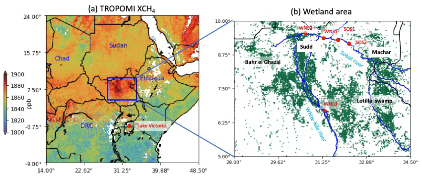
Figure 1 The TROPOMI XCH₄ enhancement over the South Sudan wetlands. (a) Average of 2 years (December 2017 to November 2019) of TROPOMI XCH₄ at 0.1^∘ × 0.1^∘ resolution. (b) Wetlands in South Sudan from Gumbricht et al. (2017) are shown in green, and the rivers in the region are shown in blue. The area within the blue rectangle (5–10^∘ N and 28–34.5^∘ E) is referred to as the South Sudan wetlands region (SSWR). The red dots show the locations of satellite-altimetry-based river water height measurement sites.

2.4 Emission quantification method

The wetland distribution from Gumbricht et al. (2017) is shown in Fig. 1 for the region in South Sudan where a large TROPOMI XCH₄ enhancement can be observed. This region, which includes Sudd, Machar and other smaller wetlands, is hereafter referred to as the South Sudan wetland region (SSWR). To calculate emissions, we first prepare seasonally averaged TROPOMI XCH₄ maps on a grid of 0.1^∘ × 0.1^∘ resolution. Only grid cells with at least five high-quality TROPOMI measurements are used in the season average map. We apply the mass balance method of Buchwitz et al. (2017) to calculate emissions from December 2017 to November 2019. The emission Q (Tg yr⁻¹) from the SSWR box in Fig. 1a for a given period is calculated using the following equation:

$$\begin{array}{}\text{(1)}& Q=\mathrm{\Delta }{\mathrm{XCH}}_{\mathrm{4}}\times M\times M_{\exp }\times L\times V\times C,\end{array}$$

where ΔXCH₄ is the “source XCH₄ enhancement”, i.e., the mean XCH₄ difference between the source and the surrounding background. C is a dimensionless factor of 2.0 derived by Buchwitz et al. (2017) based on the concentration difference of air parcels before and after entering a source area. M ($\mathrm{5.345}\times {\mathrm{10}}^{-\mathrm{6}}$ Tg CH₄ km⁻² ppb⁻¹) is the atmospheric total column mixing ratio to mass conversion factor for a standard surface pressure of 1013.25 hPa, which is the standard atmospheric pressure. M_exp is a dimensionless factor used to correct for the changes in column air mass with surface elevation, calculated as the ratio of surface pressure in the source and standard atmospheric pressure. L is the “effective size” of the source region (632 km), calculated as the square root of its area (4.0 × 10⁵ km²). V (km yr⁻¹) is the ventilation wind speed derived from the ERA5 meteorological reanalysis vertical wind speed profile. Surface elevation variations change the contribution of tropospheric to the total atmospheric column, which influences XCH₄. TROPOMI XCH₄ maps are corrected for this effect by adding the correction factor 7 ppb km⁻¹ from Buchwitz et al. (2017) using the GMTED2010 elevation data shown in Fig. A1 (Danielson et al., 2011). We remove the large-scale latitudinal XCH₄ gradient from the seasonal average TROPOMI XCH₄ maps by subtracting a third-order polynomial fit from the background region, excluding the source region (see Fig. 2a).

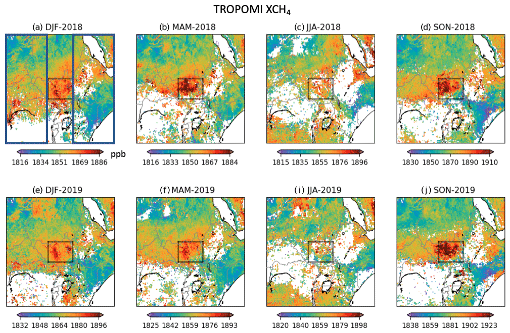
Figure 2 Seasonally averaged TROPOMI XCH₄ (ppb) at 0.1^∘ × 0.1^∘ resolution. The black rectangle at the center of each panel shows the SSWR source region. The area outside it is used as the background region. XCH₄ is corrected for large-scale latitudinal variations by subtracting a third-order polynomial fit using the region shown by blue rectangles in panel (a). The region excludes the longitudes of the source region. Note that DJF includes December of the previous year.

Figure 3 shows the monthly average ERA5 wind speed at 10:00 UTC (TROPOMI overpass time) in the SSWR as a function of pressure within the local boundary layer during select months. To calculate V, the pressure-weighted average of these boundary layer wind speeds is calculated over SSWR using monthly average ERA5 boundary layer height data. We use average boundary layer winds instead of 10 m winds because they were found to better represent the ventilation wind speed in the source region (see Varon et al., 2018). For SSWR, the 10 m wind speed is on average 35 % lower than the boundary layer wind speed, consistent with the diminishing influence of the surface friction with height.

The uncertainty of Q is calculated as the sum in quadrature of uncertainties associated with ΔXCH₄ and V. The ΔXCH₄ uncertainty is estimated as the sum in quadrature of (1) 1 SD of ΔXCH₄ estimates calculated by sequentially increasing the size of the background box from 1 to 10^∘ longitude and latitude in 1^∘ intervals and (2) the XCH₄ uncertainty of a single 0.1^∘ × 0.1^∘ grid cell on the average map (22 ppb), taken as 1 SD XCH₄ of all the grid cells in Fig. 1a. Note that this approach overestimates the XCH₄ uncertainty of the grid cells as XCH₄ variations within the grid are also caused by emissions and surface elevation variations in addition to measurement errors. The uncertainty of V is estimated from the variation in wind speed during a consecutive 4 h period (09:00, 10:00, 11:00, 12:00 UTC) centered around the TROPOMI overpass time. Note that we use the mass balance method equation from Buchwitz et al. (2017), but not their empirical equation, to estimate the uncertainty of Q. They derive that equation using a fixed wind speed of 1.1 m s⁻¹ globally, which would give a larger uncertainty in comparison to our approach of using location- and time-specific wind information: ERA5 average V is 2.5 ± 0.42 m s⁻¹ in SSWR during 2018–2019.

3 Results

3.1 XCH₄ enhancements

We first assess the XCH₄ enhancements over South Sudan from the 2-year average map of TROPOMI XCH₄ shown in Fig. 1a in relation to the SSWR wetland distribution in Fig. 1b. Similar to previous remote sensing studies (Frankenberg et al., 2011; Lunt et al., 2019; Hu et al., 2018), we observe a large XCH₄ enhancement over the Sudd wetlands. In addition, the TROPOMI data also resolve another distinct enhancement over the Machar and Lotilla wetlands in eastern South Sudan, indicating large emissions from these wetlands too. The second enhancement was also observed by Hu et al. (2018) using 2 months of TROPOMI XCH₄.

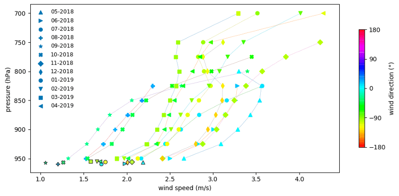
Figure 3 Monthly average boundary layer ERA5 winds in SSWR. Wind speeds (x axis) and directions (color of the markers) at 10:00 UTC, which is the closest hour to the local TROPOMI overpass time, are shown at different pressure levels of the model. The markers with dark edges represent 10 m height winds.

The Sudd wetlands are flooded by the main White Nile tributary originating from Lake Victoria, whereas the wetlands in southeast Sudan are along smaller rivers like the Kangen and Sobat, originating from the Ethiopian mountains. Lunt et al. (2019) attributed their GOSAT inversion emission estimates only to Sudd and evaluated the emissions using auxiliary data for Sudd. However, as the wetlands in the east are flooded by a different set of rivers and have a substantial contribution to the overall XCH₄ enhancement, they also need to be considered when studying the mechanisms driving the large emissions in this region.

The XCH₄ enhancement for SSWR in the 2-year average is 18.8 ± 2.8 ppb, which is more than 3 times the enhancement over the Permian basin in the USA as reported by Zhang et al. (2020). It is very unlikely that the SSWR enhancement is an artifact of the known aerosol or surface albedo biases in the TROPOMI XCH₄ data. We elaborate further on this in Appendix A. Figure 2 shows seasonally average XCH₄ maps over SSWR, and Table 1 quantifies the seasonal XCH₄ enhancement and areal coverage of the TROPOMI data. TROPOMI has good coverage in SSWR, ranging from 40 % in JJA to >90 % in DJF. It is higher than 70 % in all seasons except JJA, likely due to persistent cloud cover during the wet season. The lowest enhancements are observed in JJA in both 2018 (10.5 ± 4.1 ppb) and 2019 (2.6 ± 3.7 ppb). It is unlikely that these low enhancements are artifacts of the low coverage as there are still sufficient TROPOMI data (>40 %) and measurements are not systematically missing over the large emissions areas of SSWR, which are the Sudd and Machar wetlands. SON 2019 has the largest enhancement of 29.3 ± 4.0 ppb, likely due to low wind speeds.

Table 1 SSWR XCH₄ enhancement and emission estimates. The enhancements (ΔXCH₄) are the XCH₄ difference between SSWR and the background after correcting XCH₄ for latitudinal variations. Data coverage is defined here as the fraction of 0.1^∘ × 0.1^∘ grid cells in SSWR with at least five high-quality TROPOMI measurement in a quarter. Wind speed is the average boundary layer wind from ERA5. Emission estimates are calculated using Eq. (1); ± represents 1σ uncertainty.

3.2 Emissions quantification

We use the mass balance method of Buchwitz et al. (2017) to estimate emissions from SSWR for each season (see Table 1). Emissions during most seasons are close to 10 Tg yr⁻¹, except for the low emissions in JJA. We find very low emissions in JJA 2019 (1.4 ± 2.1 Tg yr⁻¹), but they accommodate the season's anthropogenic emissions of about 0.48 Tg yr⁻¹ (sum of 2012 EDGAR emissions and 2016 oil and gas emissions from Scarpelli et al., 2020) and GFED biomass burning emissions (0.003 Tg yr⁻¹). Direct application of the mass balance method to the 2-year average XCH₄ map shown in Fig. 1a yields annual emissions of 10 ± 1.7 Tg yr⁻¹. However, this is likely an overestimate as the 2-year average temporally under-samples the low emissions of JJA seasons due to low coverage during these seasons. Therefore, to ensure uniform temporal sampling of all seasons, we calculate annual SSWR emissions by averaging the seasonal emission estimates, resulting in 8.2 ± 3.2 Tg yr⁻¹. Moreover, this approach is likely less sensitive to error due to the mean-of-products vs. the product-of-means effect. A caveat of the mass balance method is that it ignores two factors: (1) the influence of emissions in the background region and (2) the contribution of emissions in the source region to the background average XCH₄. Both factors increase the background XCH₄ and ignoring them results in an underestimation of the emission estimate. However, this underestimation is large when the ratio of the area of the background region to the source region is small, and as we apply the method using a large background, we do not expect a significant impact on our emission estimates.

Lunt et al. (2019) report methane emissions for all sources (including wetlands, biomass burning, anthropogenic, wild animals) from the Sudd wetlands using multiyear GOSAT inversions. Their emission estimate of 5.2–6.9 Tg yr⁻¹ for 2016 is within the uncertainty bounds of our SSWR total emission estimate of 8.0 ± 3.2 Tg yr⁻¹ for 2018–2019. Note that some difference in the emission estimates can be explained by the difference in the definition of the source region between the two studies as their region extends more north and less east than ours. TROPOMI shows a large XCH₄ enhancement over the Lotilla and Machar wetlands in the east SSWR, indicating large emissions from these wetlands. As the source region in Lunt et al. (2019) only partially covers these wetlands, our emission estimates are expected to be higher.

To calculate wetlands emissions from SSWR, we account for other methane emissions in the region using bottom-up data. According to the EDGAR (version 4.3.2; Janssens-Maenhout et al., 2017) inventory for 2012, the total anthropogenic emissions from SSWR were 0.43 Tg yr⁻¹, with enteric fermentation (0.36 Tg yr⁻¹ ) being the largest anthropogenic category. The region has small emissions from wastewater management (0.03 Tg yr⁻¹), energy for buildings (0.01 Tg yr⁻¹) and manure management (0.01 Tg yr⁻¹). EDGAR does not report any significant emissions from the fossil fuel exploitation sector in the region. Recently, Scarpelli et al. (2020) presented a new inventory for the oil and gas sector in which UNFCCC reported that national emissions are spatially allocated to the fossil fuel infrastructure. They report 0.05 Tg yr⁻¹ of emissions from SSWR in 2016. Biomass burning is the largest natural methane source after wetlands in SSWR, with average emissions of 0.20 Tg yr⁻¹ in 2018–2019 according to GFED4s (0.23 Tg yr⁻¹ in 2018, 0.16 Tg yr⁻¹ in 2019; van der Werf et al., 2017). Another significant natural source is emissions from termites (0.16 Tg yr⁻¹; Sanderson, 1996). We subtract the total of these non-wetlands emissions to calculate wetland emissions of 7.4 ± 3.2 Tg yr⁻¹ from SSWR in 2018–2019. This estimate is an order of magnitude larger than the 0.5 Tg yr⁻¹ wetlands emissions from the prominent Pantanal wetlands of South America in 2010–2018, which are estimated using GOSAT inversions by Tunnicliffe et al. (2020).

Our SSWR wetlands emission estimate of 7.4 ± 3.2 Tg yr⁻¹ can be an overestimate if the emissions from the abovementioned non-wetlands sectors are underestimated in the inventories. However, this is unlikely as it would require a very large underestimation in the inventories for the 2 years studied here. For example, for the oil and gas sector, the annual emissions (0.05 Tg yr⁻¹) would need to be underestimated by 2 orders of magnitude to have a significant error impact on the wetland emission estimates. Moreover, the strong seasonality shown by the TROPOMI emission estimates is not expected in oil and gas emissions. The SSWR biomass burning emissions are higher than other sectors, but a large underestimation in annual emissions by GFED is unlikely as it uses remote-sensing-based fire activity and vegetation productivity data. There are a large number of wild animals in the SSWR, which in total emit 0.03 Tg yr⁻¹ as per Crutzen et al. (1986). Livestock is the largest anthropogenic methane source in the SSWR: 0.36 Tg yr⁻¹ in 2012 as per EDGAR v4.3.2 and 0.37 Tg yr⁻¹ in 2015 as per EDGAR version 5 (Crippa et al., 2020). South Sudan has a large population of livestock: 7.5 million dairy cattle, 4.6 million non-dairy cattle, 13.5 million goats and 16.3 million sheep in 2018, which causes 0.63 Tg yr⁻¹ of methane emissions (FAOSTATS, 2020). This amount is twice what we use to calculate the wetlands emissions for SSWR. Manure management emissions in SSWR (0.01 Tg yr⁻¹ as per EDGAR v4.3.2) are small even though there is a large cattle population in South Sudan due to lack of effective management practices. This is reflected in the small emission factors used for manure management for the country by EDGAR; for example, the dairy cattle emission factors are 1 kg CH₄ per head for South Sudan vs. 48 kg CH₄ per head for the USA. As per FAOSTATS (2020), the total emissions from manure management of dairy and non-dairy cattle, asses, chickens, sheep and goats from the whole of South Sudan are 0.02 Tg yr⁻¹. In the extreme case that all these South Sudan emissions are located in SSWR, it would slightly reduce our wetland emission estimate but still be well within its uncertainty margin.

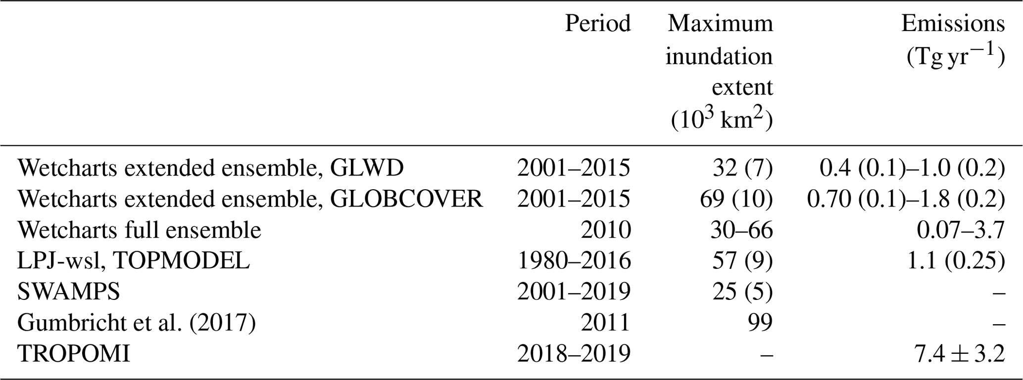
Table 2 Annual emission and maximum inundation extent estimates for SSWR. The values in parentheses show 1 SD spread over the given periods. The dashed values give the range of Wetcharts ensemble estimates.

3.3 Comparison to wetland process models

3.3.1 Annual means

SSWR integrated mean methane emission estimates from the process models are nearly an order of magnitude lower than those from TROPOMI (Table 2). For example, the multi-annual mean emissions from LPJ-wsl for 1980–2016 are 1.1 Tg yr⁻¹ (ranging from 0.5 Tg yr⁻¹ in 1990 to 1.5 Tg yr⁻¹ in 1998). The multi-annual mean individual ensemble estimates from the Wetcharts extended ensemble range from 0.4 Tg yr⁻¹ (uses GLWD) to 1.8 Tg yr⁻¹ (uses GLOBCOVER). The smallest and largest annual emission estimates from these ensemble members are 0.29 Tg yr⁻¹ in 2009 and 2.21 Tg yr⁻¹ in 2013. The Wetcharts full ensemble, with 324 estimates for 2009–2010, has a mean of 0.9 Tg yr⁻¹, ranging from 0.07 to 3.7 Tg yr⁻¹.

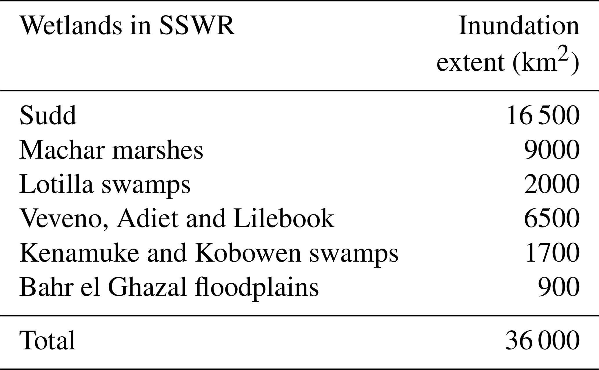
Table 2 also presents the maximum SSWR inundation extent (i.e., sum of seasonal and permanent wetland areas) used by the process models. They range from 25 000 to 69 000 km² across the models and are up to 4 times lower than the observation-based maximum inundation extent estimates of 99 000 km² by Gumbricht et al. (2017). Huges and Huges (1992) give the permanent wetland area of the different wetlands in SSWR (Table A1 in the Appendix). The sum of these areas is 36 000 km², significantly larger than the permanent inundation extent (i.e., minimum inundation extent) used in the models (Wetcharts extended ensemble: 1000 km²; LPJ-wsl: 14 000 km²; SWAMPS: 16 000 km²). Rebelo et al. (2012) used remote sensing data to characterize the inundation extent of the Sudd wetlands over a 12-month period, yielding a total wetlands area of 50 000 km² (41 000 km² seasonally inundated and 9000 km² permanently inundated). According to Huges and Huges (1992), other wetlands in the SSWR have a total permanent wetlands area of >20 500 km², meaning that Sudd accounts for only about a third of the SSWR's total wetland area. As other wetlands in SSWR are also along rivers like the Sobat, their inundation extent likely has a large seasonality, and assuming that the relative seasonal amplitude of the inundation extent of these other wetlands is similar to that of Sudd would give a total (seasonal + permanent) flooded area of 134 000 km². Adding the Sudd inundation extent yields a total SSWR inundation extent of 164 000 km², which is larger than the total estimate of 99 000 km² from Gumbricht et al. (2017). Overall, we find substantial evidence of underestimations of SSWR inundation extent in the process models, which may explain their emission underestimations as they assume that inundation extent is a strong control of the emissions.

We now look at variations in annual mean inundation extent to find a possible cause of the high emissions in 2018–2019. Lunt et al. (2019) attribute the emission increase in South Sudan between 2010 and 2016 to an inundation extent increase in the Sudd owing to increased water inflow from the White Nile River found in satellite-altimetry-based river water height measurements. To investigate this for the period 2018–2019, we look at trends in water height (see Fig. 4) of Lake Victoria as well as the White Nile and Sobat rivers. Similar to Lunt et al. (2019), we observe a rapid water height increase during 2011–2014. After this period, water levels stabilize and slightly decrease but remain significantly higher than in 2009–2010. The year 2019 shows the highest water level for the Sobat River due to a renewed positive trend from 2017 onward. This suggests that the total SSWR inundation extent was significantly higher in 2018–2019 than the pre-2011 levels. In contrast, the inundation extent data used in the process models, shown in Fig. 4a, have negative trends, which means that the process models do not account for the emission increase during 2010–2016 due to increasing inundation extent, as suggested by Lunt et al. (2019).

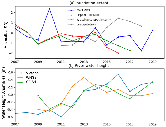
Figure 4 SSWR inundation extent estimates. (a) Annual anomalies of inundation extent estimates from SWAMPS, TOPMODEL and Wetcharts (ERA-Interim) used in process models, as well as ERA5 precipitation, expressed in units of the standard deviation of the respective annualized time series. (b) Water height anomalies for the altimetry sites in Lake Victoria as well as the White Nile (WNS3) and Sobat (SOS1) rivers from the Hydroweb database. Locations of these altimetry sites are given in Fig. 1. Here we only use the altimetry sites which have sufficiently long temporal coverage that includes 2018–2019.

Inundation extent estimates from the remote-sensing-based SWAMPS also do not show the increase and underestimate annual means. Schroeder et al. (2015) have recommended not using SWAMPS absolute inundation extent as the microwave sensors used in SWAMPS have limited capability to detect water underneath the soil surface or beneath closed forest canopies. This effect can also impact temporal changes, in addition to the absolute inundation extent, as such flooding beneath forest canopies would also not be observed. It is unclear why TOPMODEL, which accounts for lateral water transport processes, does not capture the trend in river outflow. These are interesting topics for follow-on investigations.

3.3.2 Seasonal cycle

Next, we assess the seasonal cycle of the TROPOMI-derived emission estimates. Figure 5a shows the seasonal cycles in 2018 and 2019. The largest emissions are in DJF in 2018, while DJF, MAM and SON have large emissions of similar magnitude in 2019. In both 2018 and 2019, TROPOMI emissions are lowest in JJA; in contrast, the process models estimate the lowest emissions in DJF (Fig. 5c). We investigate this mismatch by looking at the seasonal cycle of inundation extent in the models. The model emissions have a strong correlation with the inundation extent they use (Wetcharts R=0.91 and LPJ-wsl R=0.94, where R is correlation coefficient), indicating that the seasonality of emissions is driven by inundation extent. In fact, the differences in inundation extent seasonality between LPJ-wsl and Wetcharts are consistent with the emissions differences; for example, both inundation extent and emissions in LPJ-wsl are lower than in Wetcharts during MAM.

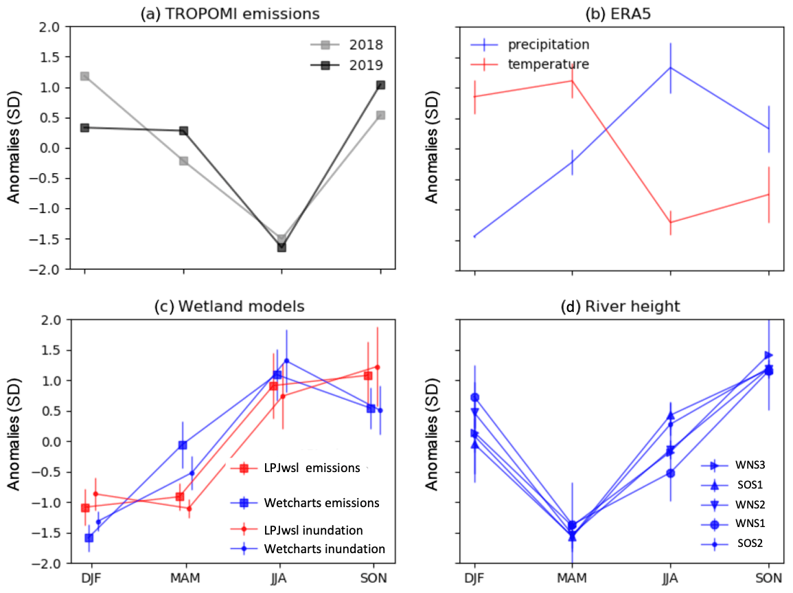
Figure 5 Mean seasonal cycles expressed in units of the standard deviation of the respective time series. (a) Emission estimates from TROPOMI; (b) precipitation and temperature from ERA5 (2010–2019); (c) emissions and inundation extent from the process models LPJ-wsl and Wetcharts extended ensemble; (d) river water height measurements at the altimetry sites given in Fig. 1b. The vertical bars represent 1 SD spread over different years.

The seasonality of the altimetry-based river water height measurements, shown in Fig. 5d, is highest in SON and is very different from the Wetcharts inundation extent (highest in JJA). This can partially explain the difference in the seasonal cycles of Wetcharts and TROPOMI emissions. The seasonal cycle of Wetcharts inundation extent is strongly correlated with local precipitation (Fig. 5b), as the intra-annual inundation extent variation is calculated using precipitation. However, this method would not accurately account for inundation extent variation due to lateral water fluxes and evapotranspiration. Surface runoff is especially important for river-fed wetlands like Sudd, whose inundation extent is controlled by water inflow from the White Nile because the evapotranspiration rate exceeds rainfall in the region (Lunt et al., 2019; Sutcliffe and Brown, 2018). LPJ-wsl inundation extent seasonality shows better agreement with the river height data as it is calculated using TOPMODEL, which accounts for lateral fluxes and evapotranspiration. However, LPJ-wsl emissions still show large differences with the seasonal cycle of TROPOMI emissions. Previous remote sensing studies for the Sudd wetlands have found the largest inundation extent during September–January in 2007–2008 (Rebelo et al., 2012) and during December–January in 1991–1992 (Travaglia et al., 1995), in better agreement with river height measurements than the process models. Overall, the inundation extent seasonality of models appears to be significantly off, which can explain part of the mismatch between TROPOMI and model emissions. In both 2018 and 2019, TROPOMI emission estimates are the lowest during JJA, while river height measurements are the lowest in MAM. A similar seasonal cycle mismatch in the GOSAT emission estimates and inundation extent, derived using MODIS land surface temperature (LST) as a proxy, is shown in Lunt et al. (2019). Furthermore, they find the highest emissions trend during SON, which had the smallest trend in inundation, but no trend in emissions during MAM, which has the highest inundation extent trend (i.e., strongest negative LST trend).

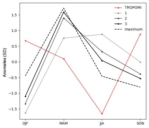
Figure 6 Seasonal cycle of SSWR emissions. Methane emissions from the Wetcharts full ensemble for 2010 (December 2009–November 2010) and TROPOMI are shown. The solid lines show the average of an emission estimate ensemble for a temperature dependency (q₁₀). The dashed line shows the seasonal cycle of the Wetcharts estimate that has the largest annual emissions. All values are shown in units of standard deviation.

An explanation for the difference in seasonal phasing can be a higher temperature dependence of emissions than suggested by the models as temperatures are lowest during JJA. We evaluate this hypothesis using the Wetcharts full ensemble, which provides a total of 324 emission estimates for three temperature dependences q₁₀ (1, 2, 3; see Bloom et al., 2017). Figure 6 compares the average seasonal cycle of TROPOMI emissions with Wetcharts emissions using different q₁₀ values (see also Table 3). Wetcharts emissions with q₁₀ = 1 have the poorest agreement with the seasonal cycle of TROPOMI ($R=-\mathrm{0.62}$). Interestingly, these emissions also have the lowest annual means (0.5 Tg yr⁻¹). Conversely, Wetcharts emissions with q₁₀ = 3 have the best correlation with TROPOMI (R = −0.28) and have the largest annual mean (1.0 Tg yr⁻¹). In fact, the member estimate – out of the 324-member full ensemble – with the largest annual emissions of 3.7 Tg yr⁻¹ has the best correlation with TROPOMI (R = 0.00). As expected, this member uses q₁₀ = 3. The agreement of TROPOMI with the larger q₁₀ model estimates, in terms of both annual mean and seasonal cycle, suggests that wetland emissions from SSWR have a large temperature dependence. In their study of wetlands in the Amazon Basin, Tunnicliffe et al. (2020) pointed to temperature as a more important control on methane emissions than inundation extent. They find a simultaneous, spatially correlated emission and temperature increase in the western Brazilian Amazon during the El Niño of 2015, with an unchanged inundation extent. Moreover, Wilson et al. (2016) found a negligible impact on wetlands emissions in the Amazon Basin despite the large difference in precipitation between 2010 and 2011, which impacted the inundation extent significantly. Note that it is also possible that the higher q₁₀ values we find for SSWR emissions are simply compensating for errors due to a misrepresentation of inundation extent or other factors covarying with temperature.

Table 3 Annual emission estimates from the Wetcharts full ensemble (2010) for different temperature dependencies and the correlation coefficient (R) of their respective average seasonal cycle with TROPOMI emissions.

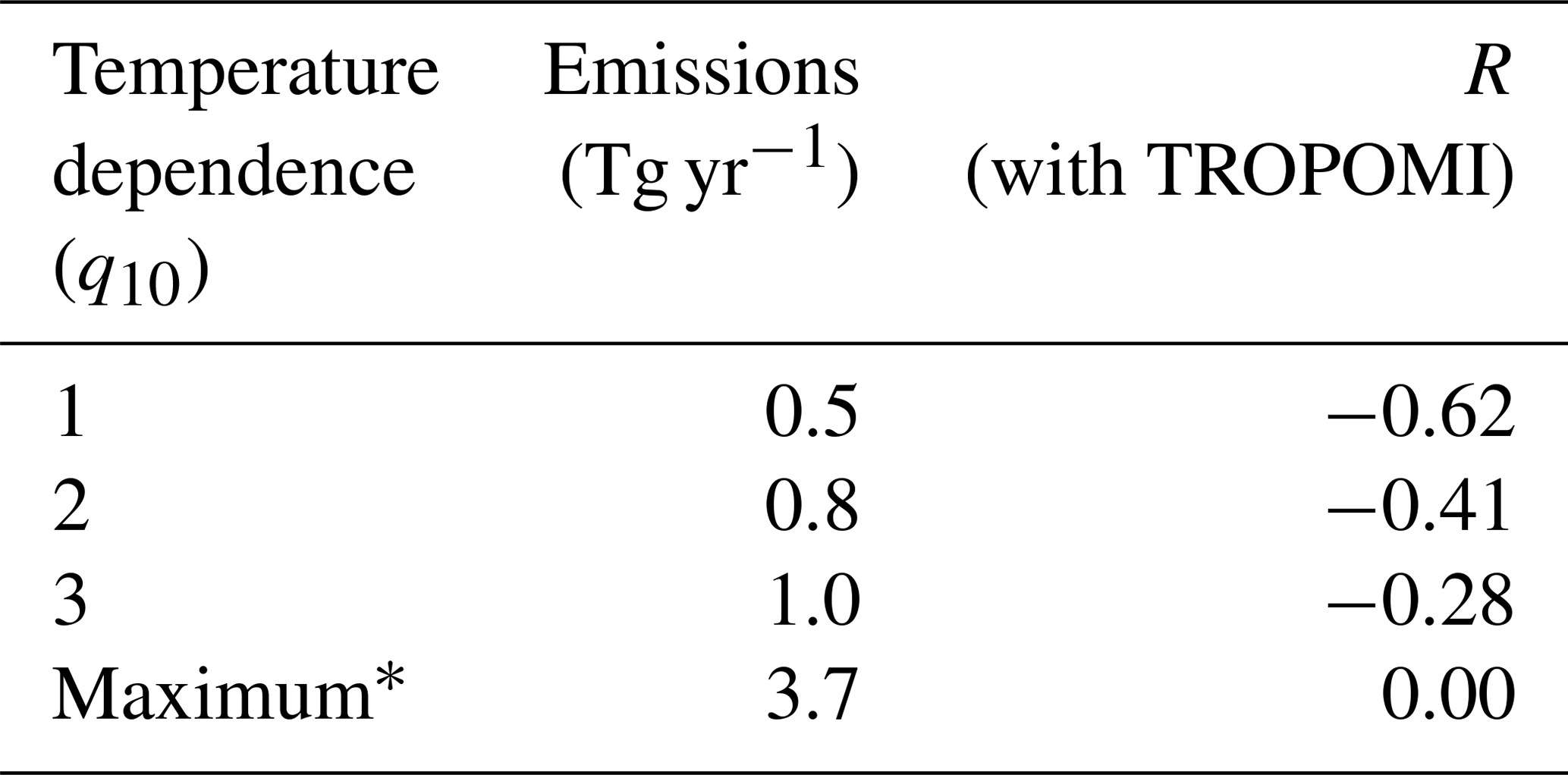
^* The maximum annual emission estimate in the 324-member ensemble of the Wetcharts full ensemble. Its q₁₀ is 3.

Figure 7 shows the emission anomaly time series from TROPOMI along with temperature and inundation extent, which we assume to be proportional to river height. A small lag between the river height and inundation extent is expected, but we expect it to be negligible in comparison to a full season. We observe that the emissions show a strong correlation with temperature (R=0.49) but a poorer correlation with inundation extent (R=0.24). The emissions peak a full season later than inundation extent, and accounting for this seasonal lag improves the correlation significantly (R=0.80). An explanation for this can be the higher temperature dependence of emissions discussed earlier. Another explanation could be the “activation” time of methanogenesis, as after flooding it takes time for anoxic conditions to develop and alternative electron acceptors to be depleted. Jerman et al. (2009) documented evidence that methane emissions from water-saturated soil slurries remained very low for a long time: methane production started after a lag of 84 d at 15 ^∘C and a minimum of 7 d at 37 ^∘C, the optimum temperature for methanogenesis. They found that the lag was inversely related to iron reduction, which is expected as iron reduction outcompeted methanogenesis. Similarly, Itoh et al. (2011) investigated methane emissions from rice paddy fields and found a time lag of a few weeks between the onset of inundation and peak emissions.

Figure 7 Seasonal anomalies in SSWR. (a) TROPOMI emissions estimates, ERA5 temperature and inundation extent from river height measurements are shown. (b) Local precipitation and SWAMPS inundation extent data are shown. All values are expressed in units of standard deviation. The correlation coefficients (R) of TROPOMI emissions with temperature, river height, SWAMPS and precipitation are 0.49 and 0.24, −0.33 and −0.67, respectively.

Process models assume that wetland emissions are instantaneously regulated by inundation extent, and they do not account for the time lag as information on the availability of alternate electron accepters is generally not available. This results in an incorrect temporal allocation of the wetland emissions. Furthermore, some models assume that inundation extent is instantaneously regulated by precipitation. In river floodplains like Sudd, inundation extent is mostly controlled by river inflow and not the local precipitation, as the evapotranspiration rates exceed rainfall in the region. Therefore, scaling with precipitation would even worsen emission estimates. Overall, a combination of temperature and inundation extent dependences that are used in the models can explain their seasonal cycle mismatch with TROPOMI emissions.

4 Conclusions

XCH₄ enhancements over South Sudan have been observed in remote sensing studies suggesting large emissions from the Sudd wetlands as the cause (Lunt et al., 2019; Hu et al., 2018; Frankenberg et al., 2011). We observe two large enhancements in the region on a 2-year average map of TROPOMI XCH₄ – over the Sudd, Machar and Lotilla wetlands. The Sudd wetlands are flooded by the White Nile River originating from Lake Victoria, while the wetlands in the east are around smaller rivers like the Sobat originating in the Ethiopian mountains. In this study, we examine these wetlands and their river systems together to understand the controls of the emissions causing the large XCH₄ enhancements.

We estimate methane emissions of 7.4 ± 3.2 Tg yr⁻¹ from wetlands in South Sudan during 2018–2019 using a mass balance approach applied to TROPOMI data. We find large differences between the emission estimates from TROPOMI and the wetland process models LPJ-wsl and Wetcharts. The annual mean estimates from TROPOMI are an order of magnitude larger than mean estimates of the models, which may be explained by the underestimated (up to 4 times) inundation extent in the models. We find differences in the interannual variability and average seasonal cycles of TROPOMI and the models, which can again be partially explained by the strong dependence of model emissions on poor inundation extent estimates. We find the lowest emission in the highest precipitation and lowest temperature season (JJA) when models estimate large emissions as they incorrectly assume an instantaneous influence of the precipitation-derived inundation extent. We find that the Wetcharts emission estimates that use a stronger temperature dependence (q₁₀ = 3) show better agreement with TROPOMI concerning both seasonality and annual emissions. This indicates that the models may also underestimate the temperature sensitivity of the methane emissions.

The inundation extent of SSWR is analyzed using satellite-altimetry-based river height measurements of the White Nile and Sobat rivers at locations within the Sudd and Machar wetlands. The inundation extent estimates used in models are based on the local precipitation, whereas the actual inundation extent of SSWR is driven by water inflow from the rivers as evapotranspiration exceeds the precipitation in the region. As a result, both the seasonal cycle and trend of model inundation extent disagree with river height data. The seasonal cycle of inundation extent from river height data shows better agreement with the TROPOMI emissions when a full season-long lag between the two is assumed. This time lag can be explained by the time needed for methanogenesis to develop in the seasonally flooded areas of the wetlands. A more precise estimate of the lag is not possible due to the coarse temporal resolution of our TROPOMI emissions estimates.

The lack of information on the correct relationship of wetland emissions to inundation extent and temperature results in large model uncertainties. Such large gaps in our understanding of the processes driving wetland emissions call for further investigation. As shown here for the wetlands of South Sudan, TROPOMI provides valuable observations over remote and inaccessible wetland regions of the world, which future wetland studies can take advantage of.

Appendix A: Systematic measurement errors

Surface albedo and aerosols can alter the optical light path, introducing biases in XCH₄ (Butz et al., 2012). Therefore, the XCH₄ enhancement over South Sudan can be affected by the differences between the source and background region values of these parameters. The average retrieved aerosol optical thickness (AOT) and surface albedo in the SWIR band of TROPOMI are shown in Fig. A1. For SSWR and its background, the AOT and albedo differences in 2-year average data are 0.001 and −0.10, respectively. The average differences for seasonal average maps are −0.01 ± 0.01, −0.15 ± 0.02 and 16.3 ± 8.4 ppb for AOT, albedo and XCH₄, respectively. The negative albedo difference for SSWR occurs due to the high albedo for the Sahara in the background. This small albedo difference is unlikely to influence the SSWR XCH₄ enhancement significantly, especially as an albedo-based bias correction is applied to the XCH₄ in the operational TROPOMI product (Hasekamp et al., 2019). We also examined the possibility that the XCH₄ enhancement over South Sudan is an artifact of the sun-glint geometry of TROPOMI observations due to reflection from standing water in the lakes and inundated areas in the region. This can happen when the observation geometry over a water body surface is at the specular reflection angle (i.e., the viewing zenith angle matches the solar zenith angle), causing a spike in the level 1 radiance measurements. However, this was found not to occur over the wetlands of South Sudan.

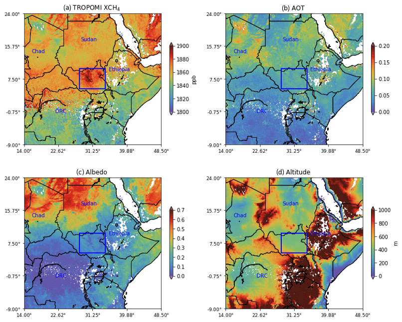
Figure A1 Average TROPOMI data (2018–2019) at 0.1^∘ × 0.1^∘ resolution. The albedo and AOT are retrieved for the SWIR band at 2.3 µm.

Table A1 The total of permanent SSWR inundation extent from Huges and Huges (1992).