the Creative Commons Attribution 4.0 License.
the Creative Commons Attribution 4.0 License.
 | 21 Oct 2021
Theoretical insights from upscaling Michaelis–Menten microbial dynamics in biogeochemical models: a dimensionless approach
Chris H. Wilson
Stefan Gerber
Leading an effective response to the accelerating crisis of anthropogenic climate change will require improved understanding of global carbon cycling. A critical source of uncertainty in Earth system models (ESMs) is the role of microbes in mediating both the formation and decomposition of soil organic matter, and hence in determining patterns of CO2 efflux. Traditionally, ESMs model carbon turnover as a first-order process impacted primarily by abiotic factors, whereas contemporary biogeochemical models often explicitly represent the microbial biomass and enzyme pools as the active agents of decomposition. However, the combination of non-linear microbial kinetics and ecological heterogeneity across space and time guarantees that upscaled dynamics will violate mean-field assumptions via Jensen's inequality. Violations of mean-field assumptions mean that parameter estimates from models fit to upscaled data (e.g., eddy covariance towers) are likely systematically biased. Likewise, predictions of CO2 efflux from models conditioned on mean-field values will also be biased. Here we present a generic mathematical analysis of upscaling Michaelis–Menten kinetics under heterogeneity and provide solutions in dimensionless form. We illustrate how our dimensionless form facilitates qualitative insight into the significance of this scale transition and argue that it will facilitate cross-site intercomparisons of flux data. We also identify the critical terms that need to be constrained in order to unbias parameter estimates.
- Article
(1618 KB) - Full-text XML
- BibTeX
- EndNote


The current crisis of anthropogenic climate change is expected to accelerate during the 21st century. Despite considerable effort to better constrain global biogeochemical models, considerable uncertainty remains about how best to represent emerging mechanistic understanding of soil element cycling into process-based models (Wieder et al., 2015; Todd-Brown et al., 2018). This is a critical gap in knowledge because variations among models predict hugely varying responses to global change drivers such as temperature, soil moisture, and CO2 enrichment. For example, a traditional first-order linear model forecasts no change or even slight enhancement of soil organic carbon (SOC) pools by 2100 whereas one microbially explicit model forecasts a loss of ∼ 70 Pg of carbon (C), depending on whether microbial physiology acclimates to higher temperatures (Wieder et al., 2013). In general, our understanding of how carbon (and other elements) cycles in soil is undergoing significant revision toward a more microbially centric paradigm. In contrast to traditional first-order linear models (e.g., CENTURY; Parton et al., 1987), microbial explicit models feature non-linear dynamics in which microbial biomass (or, similarly, microbially driven enzyme pools) is responsible for decomposition, in addition to providing substrate for synthesis of potentially long-term SOC (Blankinship and Schimel, 2018; Blankinship et al., 2018). While indisputably a better representation of our scientific knowledge, non-linear microbial models face several well-known challenges, including less analytical tractability, greater computational challenges, and uncertainty about structural formulation and dynamics (Georgiou et al., 2017; Sihi et al., 2016; Wang et al., 2014). However, one critical consequence of non-linear microbial models that has only recently begun to gain attention is their implications for addressing the upscaling challenge.
While the fields of population and community ecology have long confronted the challenges posed by non-linearity and heterogeneity in spatiotemporal scaling of ecological dynamics (Chesson, 2009; Levin, 1992), ecosystem ecology and biogeochemistry have tended to approach the challenge of scale either by (1) utilizing mean-field assumptions or (2) addressing the challenge of scaling via grid-based computational/numeric methods. While there is nothing inherently wrong with either approach, they unfortunately cannot yield theoretical insight into the consequences of non-linearity and heterogeneity for scaling. Briefly, the combination of non-linearity and heterogeneity means that aggregated behavior differs systematically from mean-field predictions, a special case of Jensen's inequality. In mathematical notation:
Although Jensen's inequality is well-known from basic probability theory (Ross, 2002) its implications for ecological dynamics under heterogeneity were not well-appreciated until the pioneering work of Peter Chesson in the 1990s (Chesson, 1998). In the case of carbon cycle science, there are a few immediate and critical applications. For instance, most trace gas emission processes are well-known to be non-linear functions of underlying drivers such as temperature and soil moisture. For example, ecosystem respiration is an exponential function of temperature (usually expressed in Q10) and a unimodal function of soil moisture. Thus, when matching observations of CO2 efflux (“F”) to ecosystems, variations in soil temperature and moisture could imply that F differs systematically from a mean-field prediction. Likewise, variations in biotic interactions between microbes likely play a key role in biogeochemical cycling (Buchkowski et al., 2017). In addition to missing critical analytical insight, not accounting for this behavior might have severe consequences for inverse modeling and estimation of the parameters governing process-based models (Bradford et al., 2021). Moreover, a significant advance in recent research has focused not only on microbially explicit formulations but also the role of microbe–substrate colocation in the complex and heterogeneous soil environment in both the synthesis and decomposition of organic matter (Schimel and Schaeffer, 2012; Lehmann et al., 2020). This spatial colocation itself has very important implications for scale transitions in soil systems and thus requires specific theoretical attention from this perspective. Overall, the basic consequences of Jensen's inequality for estimation of trace gas emission (CH4 and N2O) were first discussed by Van Oijen et al. (2017) but have not been picked up on elsewhere, until the present work and by Chakrawal et al. (2020).
Chakrawal et al. (2020) provide a detailed and compelling first-pass application of scale transition theory to biogeochemical modeling. Our contribution here complements their laudable effort by providing a more generic mathematical analysis of the scale transition, equally applicable to both forward and reverse Michaelis–Menten microbial kinetics. As in Chakrawal et al. (2020), we address the consequences of heterogeneity in both substrate/microbes (“biogeochemical heterogeneity”) and in the kinetic parameters (“ecological heterogeneity”). However, we diverge from their approach in that, rather than explore detailed simulation models, we derive a completely non-dimensionalized expression for aggregating non-linear microbial kinetics over both types of heterogeneity simultaneously. We illustrate the clarity this brings in several special cases of our full analysis. Altogether, our approach provides new insight into the properties of the scale transition and enables clear conclusions to be drawn across systems in terms of the role of spatial variances and covariances in shaping ecosystem carbon efflux. Our work provides a simplified, yet systematic framework around which to base subsequent empirical and simulation-based studies.
A variety of microbially explicit process-based models have been proposed in the literature, starting with the classic enzyme pool model of Schimel and Weintraub (2003). In order to elucidate universal properties of the scale transition, we focus here on the CO2 efflux following decomposition of a single substrate by a single microbial pool obeying Michaelis–Menten (MM) dynamics:
where F is the CO2 flux, C is the carbon substrate, MB the live microbial biomass, and θ is a vector of parameters, specifically Vmax (the maximum reaction rate given saturation of either C, in forward MM, or microbial biomass (MB), in reverse MM), kh (the half-saturation constant), and carbon-use efficiency, ϵ.
Our specific model for F is
Following the terminology of Chesson (1998, 2012), the above is our “patch” model, and our goal is to understand how spatial variances and covariances impact the integrated flux, which represents the spatial expectation or E[F] (hereafter denoted ), which represents
where the bar over the expression represents the mean. The incorrect approach to solving for E[F] is to simply plug in the mean-field solution:
Analytically, an exact solution would require specification of a joint distribution for C, MB and parameters, ), and solution of the convolution integral:
However, following Chesson (2012) and Chakrawal et al. (2019), we are free to approximate the solution for arbitrary distributions using a Taylor series approximation expanded to the second moment. Specifically, we take the expectation over a multivariable Taylor series expansion, centered around the mean-field values of all parameters θ (for simplicity, the variables MB and C are included in the parameter vector θ):
where H[f(θ)] represents the Hessian matrix of the function that determines the CO2 efflux F (in this case Michaelis–Menten), and represents the deviation from the mean at each instance and for each of the parameters. It can easily be seen that is the variance–covariance matrix and that the first moment of the Taylor expansion cancels because the first derivative of is zero.
Non-dimensionalization
Expanding Eq. (7) out, we have five terms involving the variances of C, MB, 1−ϵ, Vmax, and kh and 10 terms involving covariances among the parameters. We can redistribute the expectation operator over this approximation to see that we are dealing with the contributions from the variance–covariance terms, weighted by the second partial derivatives evaluated at the mean for each parameter. However, the resulting expression does not readily yield insight into the impact of scale transition upon the dynamics, since second partial derivatives and cross partial derivatives do not have easy intuition. Moreover, variances and covariances depend arbitrarily upon the scale of units and measurements involved, hindering both intuition and cross-site comparisons. Therefore, we non-dimensionalize Eq. (7) for as follows.
We define a dimensionless quantity λ as . λ thus represents a multiplicative factor expressing the ratio of the mean microbial biomass over its half-saturation value, indicating the microbial saturation for the decomposition.
We divide all of the terms in Eq. (6) by their mean-field value and represent the whole equation as a product:
We notice that can be re-expressed as , which in turn is the square of the dimensionless coefficient of variation (CV(θ))2. This enables us to reformulate the variance terms in Eq. (7).
Similarly, since the covariance terms can be rewritten as ), where ρX,Y is the correlation coefficient, we have the following equality:
Applying steps 1–5 to all the terms in the equation, we end up with a fully dimensionless equation:
Note that by symmetry, we have also solved for the case of the forward Michaelis–Menten kinetics. This can be expressed simply by interchanging C and MB and by correspondingly altering λ to represent the ratio of substrate availability over half saturation.
Having fully non-dimensionalized Eq. (7), we are in a much better position to gain analytical insight into the scale transition. To begin, we note the pivotal role played by the quantity λ throughout this equation. λ scales the contributions of the parameter variation and correlation terms to the deviation from mean field behavior according to the ratios , , and . All of the parameter variance terms (which have become CV(θ)2 upon non-dimensionalization) are scaled by one of these three λ ratios, alongside 7 out of 10 of the covariance terms. Overall, low λ (here ⪅1) keeps all the spatial correction terms in play, while increasing λ tends to simplify matters. As noted by others (Sihi et al., 2016; Buchkowski et al., 2017), as MB→∞ (equivalent to MB ≫kh or λ→∞), reverse Michaelis–Menten kinetics converge to first order, leaving
Accordingly, in our setup, the multiplicative factor for the scale transition correction approaches a simplified expression, as λ→∞:
This is quite remarkable. Despite invoking the situation where microbial biomass (and its enzyme supply) is effectively infinite – thus linearizing the underlying patch models – we cannot eliminate the possibility of a potentially substantial deviation from mean field when scaling decomposition kinetics. We note that in this resulting expression, we have reduced the situation to a set of three critical correlations involving two microbial physiological parameters (ϵ and Vm) and substrate availability (C). Regardless of their respective variabilities (CV terms), if these correlations are close to zero, then the whole expression converges to mean field.
Returning to the situation where λ is not large, if we ignore the correlation terms (temporarily setting to zero), we see that there are direct contributions to the scale transition from the variability in MB and kh that may, to some extent, balance each other:
Focusing on the offsetting correction terms, we can re-write as
and for the case of λ=1, this becomes
Thus, variability in the factors of soil protection that impact upon kh in practice can offset the impact of variability in microbial biomass itself.
More generally, starting with our dimensionless Eq. (10) puts modelers and empiricists in a better position to assess the quantitative significance of the scale transition correction across systems compared to expressions with opaque second partial derivatives and cross derivatives and arbitrarily scaled variance terms. By re-expressing in terms of dimensionless coefficients of variation, correlation coefficients and λ, we can plug in realistic values for variability in any relevant parameter and assess the percent effect on in terms of deviation from mean field behavior. We argue that this formulation possesses significant advantages not only in understanding how to scale flux estimates () within a site, but also going forward will help facilitate intercomparison among sites in terms of their scale-free variability. In particular, we explore variation in dominant environmental drivers of inter-site variation (temperature and soil moisture) below. But first, we analyze how the scale transition sheds new light on microbe–substrate colocation.
3.1 Spatial colocation of microbes and substrate
To illustrate these advantages in interpretability, we first take the special case of a model where we treat all parameters as constant (and known) except substrate and microbial biomass. This corresponds to setting the other CV and ρ terms to 0. In this case, we are isolating the impact of the spatial colocation of substrate and decomposers. Our equation becomes
In the case of this formulation, there is a very clear dual convergence as λ increases:
-
deviation from mean-field behavior declines, and
-
first-order kinetics are approached.
Indeed, our Eq. (16) reveals the exact speed of this convergence in terms of dimensionless λ and a balance of CV(MB), CV(C) and their correlation.
We illustrate the scale transition solutions to Eq. (16) as a function of λ for various choices of CV(C), CV(MB) and ρ in Fig. 1.
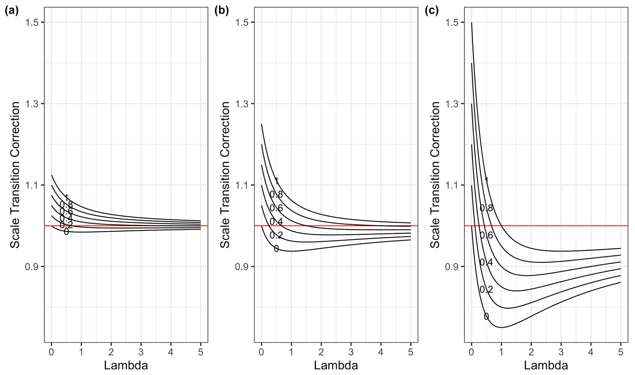
Figure 1Scale transition correction for models given spatial colocation between microbes and substrate across a gradient of λ values and for a variety of correlation ρ values (0–1), with CV(SOC) held constant at 0.5, (a) CV(MB) = 0.25, (b) CV(MB) = 0.5 and (c) CV(MB = 1. Note that in panel (c) the system appears to converge on a value lower than 1. However, as λ increases, convergence to 1 does occur, albeit slowly, as it must according to Eq. (16).
In the case of pure spatial colocation, with no variation in the kinetic parameters, the scale transition correction factor varies from a maximum of 1.5 to a minimum around 0.75 and in all cases indeed converges to 1 as λ increases. The variability assumed for C and MB impacts only the scale of the correction factor not the qualitative behavior as λ and ρ vary. One benefit of having a simplified, generic dimensionless equation of this sort is that it enables us to think in a unit-free/scale-free manner about the plausible range of the scale transition correction given transparent assumptions about variability and correlations.
Another benefit is that it is mathematically tractable to see how the variance and covariance terms can balance each other and to solve for where they are equal. If we introduce a new term λ2 representing the relationship between CV(MB) and CV(C) as follows CV(MB) =λ2CV(C), we can re-express the deviation of the mean-field correction from 1 as
Thus, whether the correction is positive or negative depends crucially on the product of the colocation correlation coefficient ρ and the extent of variability in substrate relative to variability in microbes.
If we fix λ to unity, as done in our Fig.1, our mean-field deviation simplifies to
In general, the scale transition correction is larger to the extent that microbial variability exceeds substrate variability under reverse Michaelis–Menten kinetics (the opposite relation holds for forward Michaelis–Menten by symmetry). Thus, variability in microbial biomass is not only important by itself in driving Jensen's inequality, but also with respect to variability in substrate supply. Our analysis thus highlights another route of convergence back to the mean field beyond the simple increase in λ: variability in substrate increasing to match variability in microbes in the presence of a positive spatial colocation factor. We also note that the magnitude of the scale transition correction scales as the square of the coefficient of variation in microbial biomass. Quadratic scaling means that at low to moderate levels of variability, the deviation from mean field behavior is likely to be minimal, but at moderately high to high levels of variability, severe deviations can be expected. Finally, we note that throughout, our development of these kinetics assumes proportionality to microbial biomass, but it is really the live/active fraction that matters. Since the active fraction varies considerably with environmental conditions (e.g., soil temperature and moisture explored below), we believe it is reasonable to expect large coefficients of variation overall in most real-world ecosystems.
3.2 Environmental heterogeneity
So far, we have analyzed in depth the role of variability in microbes and their substrate but not in the ecological drivers underlying maximal reaction rates (i.e., Vmax) or half saturation (i.e., kh). We start with the observation that both linear first-order and non-linear microbial models will show characteristic scale transitions given heterogeneity in temperature and soil moisture. Consider the asymptotic convergence of the reverse MM to first order:
This is mathematically equivalent to the more standard way of writing these models down as
In the analysis that follows, we will consider both temperature and soil moisture as factors that could drive variations in Vmax over space or time.
3.2.1 Scale transition over temperature heterogeneity
To make matters clear, we re-express the rate limiting maximal reaction velocity Vmax first as a function of temperature (assuming all else constant):
In this case, our integrated flux equation will be
Allowing for variability in T, this integrated equation will show characteristic scale transitions given the convex (exponential) relationship with T.
Using the Taylor expansion again to second order, we have
The critical scale transition correction term here is again multiplicative, and we re-express it into a function of a dimensionless coefficient of variation parameter more suited to ready interpretation. First, the exponential dependence of respiration on temperature is canonically codified in terms of Q10 scaling. We substitute and end up with
For a “typical” Q10 of 2.5 and a of 25, we see the multiplicative scale transition correction in Fig. 2.
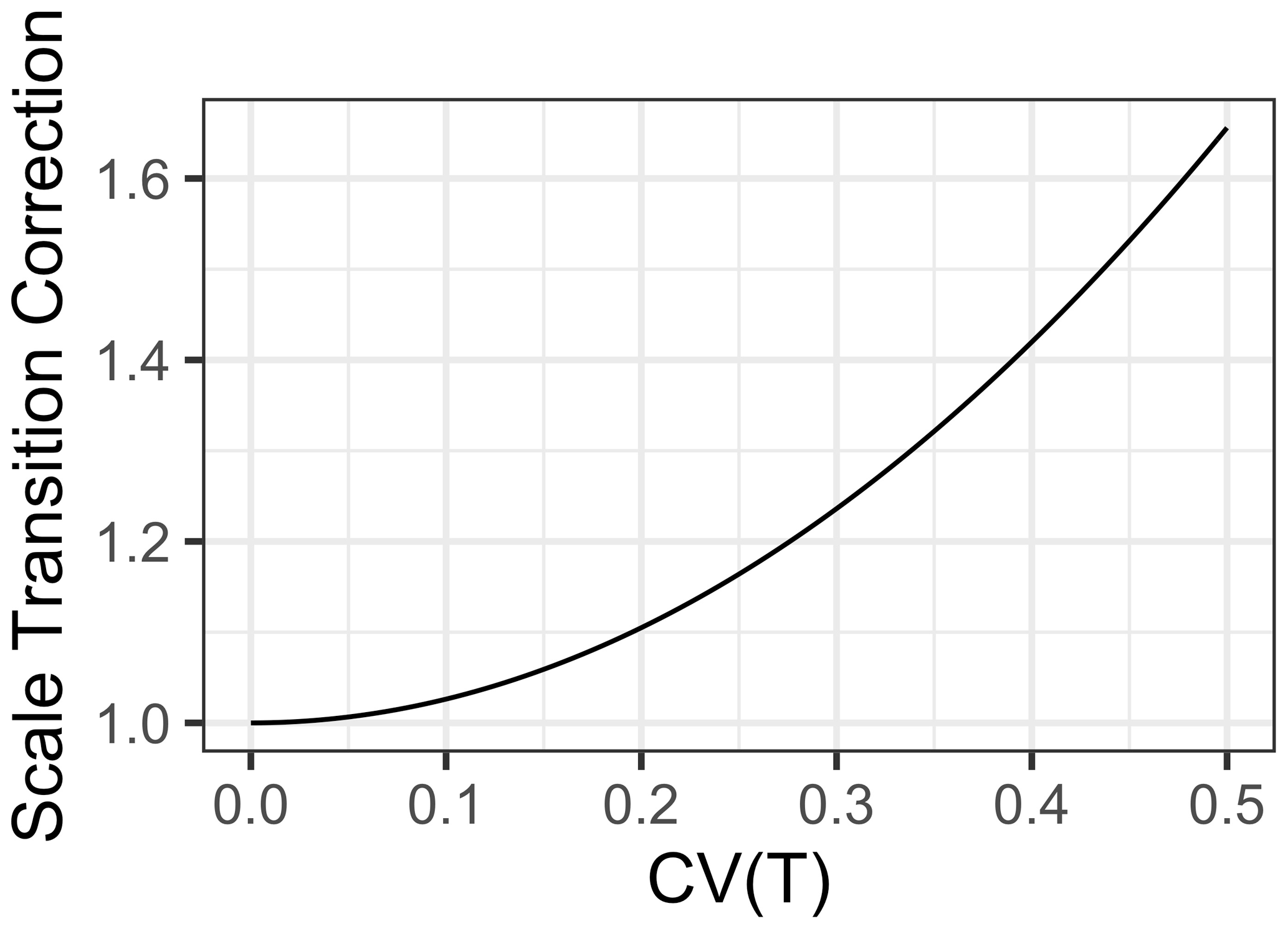
Figure 2Scale transition correction for Q10 temperature response scaling given coefficient of variation CV(Temp) from 0 to 0.5.
As is clear in Fig. 2, the scale transition for temperature is extremely convex. Integration of fluxes over ecosystems with significant heterogeneity in temperature invokes substantial deviation from a mean-field model. For instance, at a CV of 0.2, the scale transition correction is 1.10, but by a CV of 0.5 it is 1.66. Obviously, the significance of this depends on the scale and heterogeneity over which an accurate flux model is desired. For a smaller footprint eddy covariance tower (e.g., Gomez-Casanovas et al., 2018) over a uniform habitat type, soil (and near surface) temperatures probably do not vary by much more than 20 %. Regardless, our general mathematical analysis quantifies and clarifies exactly how the scale of variation influences the degree of the scale transition correction.
Notably, the only difference between the scale transition correction for first-order and for reverse Michaelis–Menten kinetics is that in the latter there would be additional correlation terms to consider, e.g., the correlation between temperature and Vmax, temperature and kh, and temperature and C and MB.
3.2.2 Scale transition over soil moisture heterogeneity
Unlike soil temperature, we expect heterotrophic respiration to respond in a unimodal fashion to soil moisture. At low levels of soil moisture, microbes are moisture limited, and at high levels they are oxygen limited, with some optimum range of values in the middle. Although a considerable amount of work has gone into developing soil moisture functions, including both empirical and theoretical derivations (Yan et al., 2018; Tang and Riley, 2019), there is no clear consensus on an optimal representation. Moreover, many of the candidate functions complicate analysis considerably by virtue of stepwise formulation (Linn and Doran, 1984). Therefore, to study the implications of the scale transition, we proceed via a powerful simplifying abstraction and simply represent the soil moisture response as a quadratic of the form
where ϕ represents the soil moisture content. We normalize our function in two senses: first in output space we assume that it has a maximum of 1 (i.e., represents heterotrophic respiration relative to a maximum value of 1) and second that the soil moisture content ϕ is itself bounded between 0 and 1, with a peak in the middle at 0.5. Thus, our function captures the unimodal abstraction in a symmetric form. Given these conditions, there is a unique solution at β=4.
We seek the scale transition:
As before, we can approximate this as a mean-field plus a correction to the mean field, which after some re-writing becomes
We then substitute Var and re-express
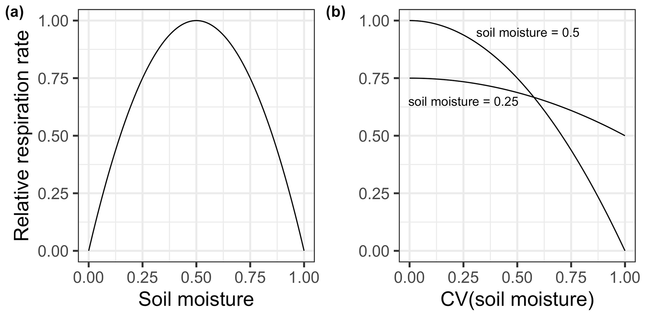
Figure 3(a) Heterotrophic respiration as a function of soil moisture given the solution in Eq. (25). Note that soil moisture is normalized with a maximum response at 0.5, where 1 represents complete waterlogging, and respiration is normalized to a maximum of 1. (b) Scale transition approximate solution for respiration as a function of the dimensionless coefficient of variation in soil moisture where mean field soil moisture is either 0.5 (top curve) or 0.25 (bottom curve, equivalent to 0.75 by symmetry).
As shown in Fig. 3, where mean field soil moisture is close to the optimal value, scale transition effects are expected to be quite large. For instance, by the time the coefficient of variation is 0.5, efflux would only be 75% and declines rapidly to 0 as the coefficient of variation approaches 1. Clearly, this latter outcome is not necessarily biologically realistic, and a more detailed numerical experiment should be done to explore scenarios with that much variation. However, our abstractions yield the simple insight that mean-field solutions invariably overestimate the real flux, and this overestimation can be considerable. In our experience, soil moisture varies tremendously both over space, especially given contrasts in topography, relief and underlying soils, and perhaps even more so over time, including within a small area, due to day-to-day and even hour-by-hour variations in precipitation, evapotranspiration and drainage. To the extent that ecosystems deviate from a stable, consistent soil moisture regime, we should expect strong scale transition effects.
Our results on soil moisture relate to the argument by Tang and Riley (2019) that heterotrophic respiration arises from a two-step process whereby substrate must diffuse into the vicinity of microbes and then be taken up – the latter by a Michaelis–Menten kinetic. However, microscale variations in soil moisture mediate and regulate the first step of the process, so that the “effective substrate affinity” (the kh term in the Michaelis–Menten model) deviates from the base substrate affinity of the second step. Tang and Riley (2019) point out that the effective substrate affinity therefore reflects microscale heterogeneity, and they argue that experimentalists should account for this when fitting efflux data to models. But what about scaling up in the field from small plots to fields to larger ecosystem units? Fortunately, our analytical framework can be readily queried to account for heterogeneity in substrate affinity (kh).
3.2.3 Heterogeneity in substrate affinity
We proceed by first holding all terms constant except allowing the half-saturation constant kh to vary, reflecting variations in soil moisture, or frankly any other factor regulating microbial access to substrate (e.g., soil aggregation, organomineral complexes, etc.; Schmidt et al., 2011; Lehmann et al., 2020). As usual, we seek the scale transition over ). We can recover this transition quickly from Eq. (10) by extracting only the term with (kh), or rederive from scratch holding everything else as constant. The result is that the dimensionless scale transition correction term is
Intriguingly, this result shows that heterogeneity in substrate affinity per se results in a convex correction term, implying that mean-field models will underestimate rather than overestimate the resulting fluxes. Given that the correction is proportional to the inverse of the square of λ, this correction converges rapidly to 1 (no scale transition) as mean microbial biomass increases (Fig. 4). Nevertheless, where heterogeneity is high and λ is around 1 or lower, the correction could be substantial.
More broadly, our analysis highlights that, under non-linear Michaelis–Menten kinetics for representing carbon processing, the impact of environmental heterogeneity acting on the substrate affinity parameter is opposite of when it acts on the Vmax parameter. Thus, if we represent soil moisture as a modifier to the Vmax in the numerator, heterogeneity in soil moisture should result in lower carbon efflux than mean field, whereas if we represent soil moisture heterogeneity by way of substrate affinity it is the opposite. At first glance, this finding appears inconsistent with Tang and Riley (2019). However, we note that their full kinetic formulations include soil moisture acting in both roles ultimately and therefore resulting in the familiar unimodal soil moisture–respiration relationship. For instance, their application of “dual Monod” kinetics includes soil moisture driving effective substrate affinity terms for both carbon and water, as well as an effective fraction of active microbes (which modifies the numerator).
Thus, for the analysis of upscaling fluxes in the presence of soil moisture heterogeneity, we expect the concave corrections of Fig. 3b to hold, regardless of the fine-scale details of the soil moisture function used.
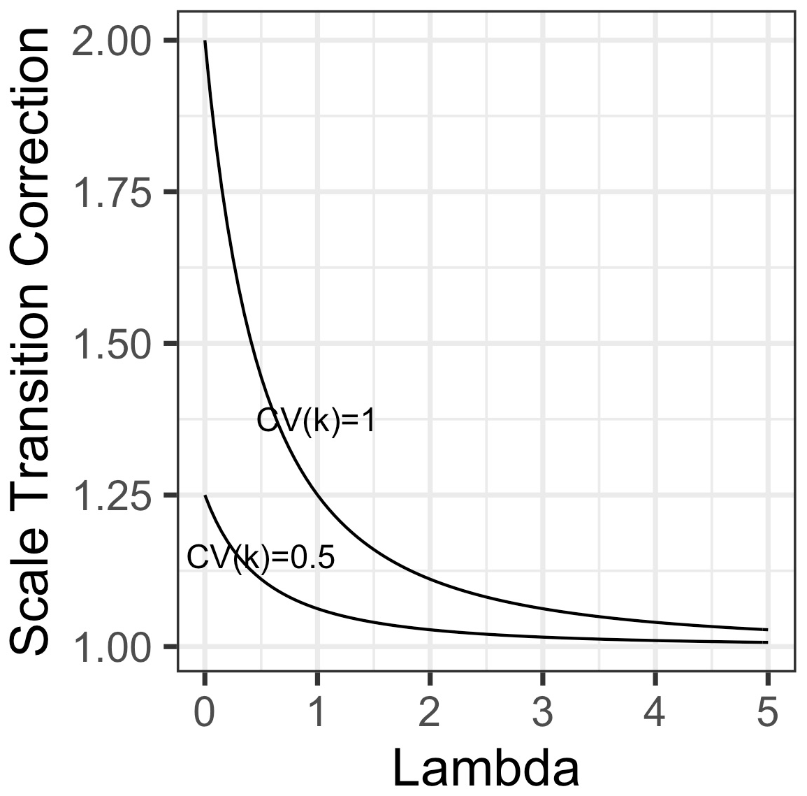
Figure 4Scale transition factor for variations in the substrate affinity (“kh”) parameter in Michaelis–Menten kinetics as a function of dimensionless λ (the ratio of mean-field microbial biomass over mean-field kh), for two scenarios of variability in affinity, one where coefficient of variation = 1 (top curve) and the other where coefficient of variation = 0.5 (bottom curve).
3.3 Lessons for scientific inference
We close our discussion by considering the implications of the scale transition for advancing the state of biogeochemical modeling. Critically, the representation of non-linear (microbial driven) kinetics is a crucial modeling choice with large implications for long-term SOC forecasts. Traditional first-order process-based models dodge explicit representation of these kinetics but nonetheless have worked well in practice. This state of affairs persists because both non-linear and linear kinetics are capable of representing coarse-scaled biogeochemistry reasonably well, at least in certain respects. Since first-order kinetics are known to be a crude approximation, the crucial question for practice is not whether they are “true”, but rather whether there is significant, systematic information loss inherent to their use. Fortunately, the scale transition offers a clear, clean path to discriminate between these alternative model formulations.
As noted throughout, the dimensionless term λ plays a critical role in linking the non-linear (Michaelis–Menten) kinetics to the first-order kinetics. As λ increases, the non-linear kinetics converge to first order. Thus, in seeking to infer where the non-linear kinetic models provide substantial advantages, ensuring that λ is not too large (≫1) is the first priority.
Previous work (Sihi et al. 2016) has approached this question theoretically, from first principles. Here, we point out that demonstrating substantial deviation from the mean-field model when fitting non-linear kinetics to data is both a necessary and sufficient condition for inferring that λ is not too large. Thus, we recommend that time series of flux data be fit to both a first-order and a non-linear kinetic model, where crucial covariates including substrate (SOC), microbial biomass and possibly environmental parameters such as temperature have been measured sufficiently well to quantify the relevant variances and covariances. Where predictive performance and forecasting are the primary goals, we recommend careful consideration of model parameterizations (i.e., based on leave-one-out cross validation) and model combination via “stacking” where it is difficult to infer a decisive “winner” (Yao et al., 2018), acknowledging that carrying this out is a significant enterprise.
In addition to the role of λ, our analysis also cleanly shows the contribution of other terms to the scale transition, and thus alternative metrics to assess. First and foremost, account for the spatial colocation of microbial biomass and substrate (according to Eq. (16) above) or the various correlation terms between microbial biomass and kinetic/environmental factors in Eq. (10). Moreover, recent theoretical developments offer quantitative insights into the interpretation of the half-saturation constant (or the substrate affinity parameter) and thus λ (Tang and Riley, 2019). Tang and Riley (2019) decompose microbial access to substrate into a two-step process, which is often strongly modified by soil moisture. Moreover, conceptual advances suggest that colocation is a potentially important factor in organic matter decomposition vs. stabilization (Schimel and Schaeffer, 2012; Lehmann et al., 2020). Here, we show that both affinity and colocation are co-dependent in their effects on scale transition.
In addition to fitting fully parameterized flux models (as above), simpler statistical models could be fit examining the role of variations in microbial biomass, or colocation of microbial biomass and SOC, in explaining across-site variations in ecosystem respiratory fluxes (F). A substantial role for either correlation of MB and C or their variability would constitute ipso facto evidence of the preferability of well-formulated non-linear kinetic models. On the other hand, small roles for colocation or evidence of large values of λ in practice would suggest a minimal advantage to abandoning first-order models in favor of more complex microbial models. A meta-analytical approach across sites will benefit greatly from our formulation in terms of dimensionless quantities like λ and the various coefficients of variation.
We further note that the scale transition presented here is closely related to global sensitivity analysis (GSA; Saltelli et al., 2010). In its fundamental setup, a GSA tests effects of variability in parameters. While GSA has been typically used towards characterizing the uncertainty of parameters, it is directly applicable to spatial and temporal variability. For example, the first-order results of a GSA (or the result of one at a time parameter substitution) provide the contribution of that parameter to the scale transition. Similarly, the “all but one” perturbation offers insights into how the net effect of all parameters (and variables) violates the mean field approximation. Therefore, a computationally expensive GSA can be leveraged to garner further insights on top of sensitivity effects, allowing for the characterization of the scale transition. Indeed, a computationally intensive approach to simulating scale transitions was utilized by Chakrawal et al. (2020) to good effect. However, we suggest future computational studies build off of the dimensionless approach studied here, including those extended to multiple microbial populations which would result in multiple dimensionless lambdas and corresponding multiplicative contributions to the scale transition. Obviously, the parameter space needs to be properly chosen (or subsetted) to reflect appropriate means, variabilities and perhaps most challenging – correlations. Equation (10) would then provide analytical, albeit approximate, insight into the scale transition effects, while the GSA would enable study of any shortcomings from approximation and also allow for quantification of individual variable importance for those parameters that enter into the dynamics in multiple places.
Finally, our analysis of environmental factors including temperature and soil moisture leads to readily testable predictions. For temperature, the scale transition is convex, and thus, ceteris paribus, variation in soil temperature should lead to greater effluxes than mean field models would predict. The implications of this for climate feedback should be studied in greater detail. For soil moisture, which varies considerably across both space and especially time, our analysis based on an idealized quadratic representation yields a concave scale transition correction, i.e., the mean-field soil moisture will overestimate efflux. Likewise, when represented in both substrate affinity and multiplicative active microbial biomass fraction terms, as in Tang and Riley (2019), the scale transition remains concave. However, environmental factors that act only through substrate affinity would result in a convex correction as in Fig. 4. Once again, we highlight that the nature of scaling corrections, wherever it is possible to be studied empirically, can provide insight into the most productive representations of our models.
Here, we have illustrated how the spatial scale transition can be expressed in dimensionless form, yielding insight into the systematic operation of Jensen's inequality in upscaling microbial decomposition kinetics. Our analysis has identified the central role of the dimensionless quantity λ – representing the ratio of mean-field microbial biomass over its half-saturation value – in governing the extent of the scale transition correction, expressed here in multiplicative form best facilitating comparison among systems. For somewhat simplified scenarios – such as restricting to spatial colocation of substrate and microbes – as λ→∞, the mean-field correction goes to 0, and the model converges to first order.
This dual sense of convergence also provides opportunity to empirically test for the presence of significant non-linear microbial dynamics in upscaled field data: to the extent that upscaled fluxes deviate from the flux estimated at mean-field conditions, we have ipso facto evidence for the importance of formulating our biogeochemical models with these non-linear terms. Conversely, where there is close agreement between mean-field and upscaled fluxes, there are arguably stronger reasons for retaining first-order process model formulations.
In closing, we would like to point out how this mathematical analysis illustrates the challenge of scaling quite nicely. In the context of non-linear models, for each parameter that is allowed to vary in space, there is not only a new variance parameter, but also a number of new covariance terms are induced, growing as the factorial of the number of varying parameters (Fig. 3). Thus, in the case of the five-parameter function considered here, the full approximation has 5 mean field terms, 5 coefficients of variation, 10 correlation coefficients and the dimensionless quantity λ.

Figure 5Model complexity grows exponentially with number of spatially varying parameters. We argue to keep models as simple as possible for both analytical and computational tractability.
Even with a maximally generic and simplified expression, fitting such non-linear time series models to field data still represents quite a challenge, especially while adequately accounting for and propagating uncertainty. Modelers and theoreticians should appreciate the complexity of the task at hand. Fortunately, our analysis has identified a potentially robust route to limiting model complexity: screen systematically for the importance of various correlations in explaining variations in fluxes. Accordingly, we recommend that research focus first upon spatial colocation of MB and C, which is readily measured, and then to thoughtfully and carefully expand models with additional terms as needed.
All code used to generate the figures in this paper, which visualize our theoretical results and mathematical derivations, is publicly available at the first author's GitHub repository here: https://github.com/chwilson/Biogeosciences_Scale_Transition (Wilson, 2021).
No data sets were used in this article.
CHW conceived the original concept, developed the mathematical analysis and wrote the manuscript. SG developed the concepts, contributed to the mathematical analysis, and co-authored and edited the manuscript.
The contact author has declared that neither they nor their co-author has any competing interests.
Publisher’s note: Copernicus Publications remains neutral with regard to jurisdictional claims in published maps and institutional affiliations.
We stand on the shoulders of giants: Peter Chesson's research program on scale transition was enormously influential. We thank Timothy Trevor Caughlin for introducing us to Chesson's papers many years ago and everyone who has humored discussions of Jensen's inequality ever since. Will Wieder and the anonymous reviewer provided constructive reviews that improved our manuscript, and Kathe Todd-Brown provided valuable discussion as we worked through revisions.
This paper was edited by Jens-Arne Subke and reviewed by William Wieder and one anonymous referee.
Blankinship, J. C. and Schimel, J. P.: Biotic versus Abiotic Controls on Bioavailable Soil Organic Carbon, Soil Systems, 2, 10, https://doi.org/10.3390/soilsystems2010010, 2018.
Blankinship, J. C., Berhe, A. A., Crow, S. E., Druhan, J. L., Heckman, K. A., Keiluweit, M., Lawrence, C. R., Marín-Spiotta, E., Plante, A. F., Rasmussen, C., Schädel, C., Schimel, J. P., Sierra, C. A., Thompson, A., Wagai, R., and Wieder, W. R.: Improving understanding of soil organic matter dynamics by triangulating theories, measurements, and models, Biogeochemistry, 140, 1–13, https://doi.org/10.1007/s10533-018-0478-2, 2018.
Bradford, M. A., Wood, S. A., Addicott, E. T., Fenichel, E. P., Fields, N., González-Rivero, J., Jevon, F. V., Maynard, D. S., Oldfield, E. E., Polussa, A., Ward, E. B., and Wieder, W. R.: Quantifying microbial control of soil organic matter dynamics at macrosystem scales, Biogeochemistry, 156, 19–40, https://doi.org/10.1007/s10533-021-00789-5, 2021.
Buchkowski, R. W., Bradford, M. A., Grandy, A. S., Schmitz, O. J., and Wieder, W. R.: Applying population and community ecology theory to advance understanding of belowground biogeochemistry, Ecol. Lett., 20, 231–245, https://doi.org/10.1111/ele.12712, 2017.
Chakrawal, A., Herrmann, A. M., Koestel, J., Jarsjö, J., Nunan, N., Kätterer, T., and Manzoni, S.: Dynamic upscaling of decomposition kinetics for carbon cycling models, Geosci. Model Dev., 13, 1399–1429, https://doi.org/10.5194/gmd-13-1399-2020, 2020.
Chesson, P.: Spatial scales in the study of reef fishes: A theoretical perspective, Ecol. Lett., 23, 209–215, https://doi.org/10.1111/j.1442-9993.1998.tb00722.x, 1998.
Chesson, P.: Scale transition theory with special reference to species coexistence in a variable environment, J. Biol. Dynam., 3, 149–163, https://doi.org/10.1080/17513750802585491, 2009.
Chesson, P.: Scale transition theory: Its aims, motivations and predictions, Ecol. Complex., 10, 52–68, https://doi.org/10.1016/j.ecocom.2011.11.002, 2012.
Georgiou, K., Abramoff, R. Z., Harte, J., Riley, W. J., and Torn, M. S.: Microbial community-level regulation explains soil carbon responses to long-term litter manipulations, Nat. Commun., 8, 1223, https://doi.org/10.1038/s41467-017-01116-z, 2017.
Gomez-Casanovas, N., DeLucia, N. J., Bernacchi, C. J., Boughton, E. H., Sparks, J. P., Chamberlain, S. D., and DeLucia, E. H.: Grazing alters net ecosystem C fluxes and the global warming potential of a subtropical pasture, Ecol. Appl., 28, 557–572, https://doi.org/10.1002/eap.1670, 2018.
Lehmann, J., Hansel, C. M., Kaiser, C., Kleber, M., Maher, K., Manzoni, S., Nunan, N., Reichstein, M., Schimel, J. P., Torn, M. S., Wieder, W. R., and Kögel-Knabner, I.: Persistence of soil organic carbon caused by functional complexity, Nat. Geosci., 529–534, https://doi.org/10.1038/s41561-020-0612-3, 2020.
Levin, S. A.: The problem of pattern and scale in Ecology: the Robert H. MacArthur award lecture, Ecology, 73, 1943–1967, https://doi.org/10.2307/1941447, 1992.
Linn, D. M. and Doran, J. W.: Effect of Water-Filled Pore Space on Carbon Dioxide and Nitrous Oxide Production in Tilled and Nontilled Soils, Soil Sci. Soc. Am. J., 48, 1267–1272, https://doi.org/10.2136/sssaj1984.03615995004800060013x, 1984.
Parton, W. J., Schimel, D. S., Cole, C. V., and Ojima, D. S.: Analysis of factors controlling soil organic matter levels in Great Plains grasslands, Soil Sci. Soc. Am. J., 51, 1173, https://doi.org/10.2136/sssaj1987.03615995005100050015x, 1987.
Ross, S.: A first course in probability, Pearson Education India, 2002.
Saltelli, A., Annoni, P., Azzini, I., Campolongo, F., Ratto, M., and Tarantola, S.: Variance based sensitivity analysis of model output. Design and estimator for the total sensitivity index, Comput. Phys. Commun., 181, 259–270, 2010.
Schmidt, M. W. I., Torn, M. S., Abiven, S., Dittmar, T., Guggenberger, G., Janssens, I. A., Kleber, M., Kögel-Knabner, I., Lehmann, J., Manning, D. A. C., Nannipieri, P., Rasse, D. P., Weiner, S., and Trumbore, S. E.: Persistence of soil organic matter as an ecosystem property, Nature, 478, 49–56, https://doi.org/10.1038/nature10386, 2011.
Sihi, D., Gerber, S., Inglett, P. W., and Inglett, K. S.: Comparing models of microbial–substrate interactions and their response to warming, Biogeosciences, 13, 1733–1752, https://doi.org/10.5194/bg-13-1733-2016, 2016.
Tang, J. and Riley, W. J.: A Theory of Effective Microbial Substrate Affinity Parameters in Variably Saturated Soils and an Example Application to Aerobic Soil Heterotrophic Respiration, J. Geophys. Res.-Biogeo., 124, 918–940, https://doi.org/10.1029/2018JG004779, 2019.
Todd-Brown, K., Zheng, B., and Crowther, T. W.: Field-warmed soil carbon changes imply high 21st-century modeling uncertainty, Biogeosciences, 15, 3659–3671, https://doi.org/10.5194/bg-15-3659-2018, 2018.
Van Oijen, M., Cameron, D., Levy, P. E., and Preston, R.: Correcting errors from spatial upscaling of nonlinear greenhouse gas flux models, Environ. Model. Softw., 94, 157–165, https://doi.org/10.1016/j.envsoft.2017.03.023, 2017.
Wang, Y. P., Chen, B. C., Wieder, W. R., Leite, M., Medlyn, B. E., Rasmussen, M., Smith, M. J., Agusto, F. B., Hoffman, F., and Luo, Y. Q.: Oscillatory behavior of two nonlinear microbial models of soil carbon decomposition, Biogeosciences, 11, 1817–1831, https://doi.org/10.5194/bg-11-1817-2014, 2014.
Wieder, W. R., Bonan, G. B., and Allison, S. D.: Global soil carbon projections are improved by modelling microbial processes, Nat. Clim. Change, 3, 909–912, https://doi.org/10.1038/nclimate1951, 2013.
Wieder, W. R., Allison, S. D., Davidson, E. A., Georgiou, K., Hararuk, O., He, Y., Hopkins, F., Luo, Y., Smith, M. J., Sulman, B., Todd-Brown, K., Wang, Y.-P., Xia, J., and Xu, X.: Explicitly representing soil microbial processes in Earth system models, Global Biogeochem. Cy., 29, 2015GB005188, https://doi.org/10.1002/2015GB005188, 2015.
Wilson, C. H.: Biogeosciences_Scale_Transition, Github [code], available at: https://github.com/chwilson/Biogeosciences_Scale_Transition, last access: 18 October 2021.
Yan, Z., Bond-Lamberty, B., Todd-Brown, K. E., Bailey, V. L., Li, S., Liu, C., and Liu, C.: A moisture function of soil heterotrophic respiration that incorporates microscale processes, Nat. Commun., 9, 2562, https://doi.org/10.1038/s41467-018-04971-6, 2018.
Yao, Y., Vehtari, A., Simpson, D., and Gelman, A.: Using stacking to average bayesian predictive distributions, Bayesian Anal., 13, 917–1007, https://doi.org/10.1214/17-BA1091, 2018.