the Creative Commons Attribution 4.0 License.
the Creative Commons Attribution 4.0 License.
 | 26 Oct 2021
Model simulations of arctic biogeochemistry and permafrost extent are highly sensitive to the implemented snow scheme in LPJ-GUESS
Alexandra Pongracz
David Wårlind
Paul A. Miller
Frans-Jan W. Parmentier
The Arctic is warming rapidly, especially in winter, which is causing large-scale reductions in snow cover. Snow is one of the main controls on soil thermodynamics, and changes in its thickness and extent affect both permafrost thaw and soil biogeochemistry. Since soil respiration during the cold season potentially offsets carbon uptake during the growing season, it is essential to achieve a realistic simulation of the effect of snow cover on soil conditions to more accurately project the direction of arctic carbon–climate feedbacks under continued winter warming.
The Lund–Potsdam–Jena General Ecosystem Simulator (LPJ-GUESS) dynamic vegetation model has used – up until now – a single layer snow scheme, which underestimated the insulation effect of snow, leading to a cold bias in soil temperature. To address this shortcoming, we developed and integrated a dynamic, multi-layer snow scheme in LPJ-GUESS. The new snow scheme performs well in simulating the insulation of snow at hundreds of locations across Russia compared to observations. We show that improving this single physical factor enhanced simulations of permafrost extent compared to an advanced permafrost product, where the overestimation of permafrost cover decreased from 10 % to 5 % using the new snow scheme. Besides soil thermodynamics, the new snow scheme resulted in a doubled winter respiration and an overall higher vegetation carbon content.
This study highlights the importance of a correct representation of snow in ecosystem models to project biogeochemical processes that govern climate feedbacks. The new dynamic snow scheme is an essential improvement in the simulation of cold season processes, which reduces the uncertainty of model projections. These developments contribute to a more realistic simulation of arctic carbon–climate feedbacks.
- Article
(7180 KB) - Full-text XML
-
Supplement
(4857 KB) - BibTeX
- EndNote


The Arctic is undergoing rapid warming, with some of the most pronounced changes occurring during the winter (Box et al., 2019; Natali et al., 2019). As a result, snow thickness, the extent of snow-covered area, and snow season length are decreasing, and this is expected to continue in the future (AMAP, 2017; IPCC, 2014). Snow is an important abiotic component of the Arctic system, since it provides an insulating cover for vegetation and soil. Snow insulation is recognized as the primary control over soil thermodynamics (Lawrence and Slater, 2010), and soil temperature is closely connected to physical (i.e. permafrost active layer depth) and biogeochemical (i.e. decomposition, greenhouse gas emission) processes (Peng et al., 2016). Observations show that snow cover changes have played a major role in a warming trend of permafrost soils of approximately 0.3 ∘C per decade (Biskaborn et al., 2019; AMAP, 2017). This warming may lead to increased microbial activity, decomposition rates and bioavailability of previously frozen soil carbon. Since permafrost soils contain approximately 1600 Pg carbon, accounting for half of the global soil carbon storage (Hugelius et al., 2014), there is ample potential for these changes to lead to the release of the greenhouse gases CO2 and methane. This has the potential to accelerate global warming (Schuur et al., 2015), which underlines the need for a better understanding of drivers and potential feedbacks to better predict the rate and magnitude of future carbon exchange.
Despite numerous field-based and modelling efforts to date, it is still uncertain whether the Arctic will act as a carbon source or sink in the future (McGuire et al., 2012; Virkkala et al., 2021). The predicted future carbon balance varies widely among models – between a loss of 641 Pg C and a gain of 167 Pg C under RCP8.5 (McGuire et al., 2018) – depending on the representation and level of detail of key processes such as soil temperature and vegetation dynamics (Schuur et al., 2015; McGuire et al., 2018). One of the key goals of model development is to decrease uncertainty of simulations by refining these processes. While extensive research has been carried out on the mechanics of the growing season, few studies have been directed at cold season processes. Recent studies suggest that the contribution of the non-growing season to the annual carbon budget may have been underestimated (Pirk et al., 2015; Mastepanov et al., 2013). A recent meta-analysis by Natali et al. (2019) found significant wintertime carbon loss and highlighted the large spread in model simulations of non-growing season greenhouse gas emissions. Models generally underestimated the observed winter flux emissions due to the inaccuracies in their simulation of cold season respiration. Natali et al. (2019) stress the need to revise the impact of environmental drivers and feedbacks in models. Collectively, these efforts demonstrate that the influence of cold season processes on the annual carbon balance is larger than previously suggested.
The ability of models to simulate physical and biological processes in the soil is limited by the complexity of their representation of snow. A recent snow-related model evaluation project analysed the performance of models with different complexity – focusing on variables such as snow-covered area and snow season length. This SNOWMIP found that a dynamic simulation of internal snowpack processes, such as density and temperature calculations, is critical to simulate snow thermal profiles (Krinner et al., 2018). In addition, more complex snow schemes perform better when simulating cold season processes (Vionnet et al., 2012; Slater et al., 2017; Wang et al., 2016). To balance computational efficiency and the need for detail, most ecosystem models use an intermediate-complexity multi-layer snow module (Vionnet et al., 2012; Krinner et al., 2018). Such schemes may not capture fine-scale internal snowpack processes such as the evolution of high-density wind slab layers, but they are complex enough to simulate key physical processes – compaction, freeze–thaw cycles, and liquid water retention – that influence the thermal dampening property of snow. Since LPJ-GUESS had a single-layer static snow representation, it was found to deviate from observational records of air–soil temperature relationships – simulating cooler winter conditions and performing poorly when compared to eight land surface models (Wang et al., 2016). This showed, combined with previous research, that the snow representation in LPJ-GUESS needed to be revised to better capture Arctic cold season conditions.
The primary aim of this study is to improve LPJ-GUESS's simulation of the insulating effect of snow. By developing and integrating a dynamic intermediate-complexity snow scheme, we also aim to improve the soil temperature and biogeochemistry simulation. To investigate the effect of the new snow scheme in LPJ-GUESS, we set out to quantify the impact on physical variables, i.e. the direct impact of snow insulation on soil temperature and permafrost conditions. To further evaluate the snow-related influence on biogeochemistry – such as changes in growing season length – we analyse a set of biogeochemical variables. Due to differences in soil temperature, we expect to see changes in ecosystem productivity, heterotrophic respiration, and soil carbon pools. Moreover, we analyse the changes to vegetation dynamics and composition. The updates to the model will allow us to assess other snow-related processes and feedbacks on a global scale, such as the impact on surface albedo and food access to herbivores, in the future.
LPJ-GUESS is a process-based dynamic vegetation model, widely applied on regional and global scales (Smith et al., 2001, 2014). For this study, we used a customized arctic version of LPJ-GUESS 4.0 (subversion 9905). The model simulates soil freeze–thaw processes and is applicable to studies of processes at northern high latitudes (Miller and Smith, 2012). In this study we restrict simulations to the northern circumpolar region (above 60∘ latitude) with a spatial resolution of 0.5∘ × 0.5∘. The CRUNCEP global reanalysis climate dataset version 7 was used as input for all of our model simulations (Viovy, 2016). We ran the model with a 500-year spin-up period to establish an equilibrium vegetation state and a 40 000-year offline spin-up period for soil conditions.
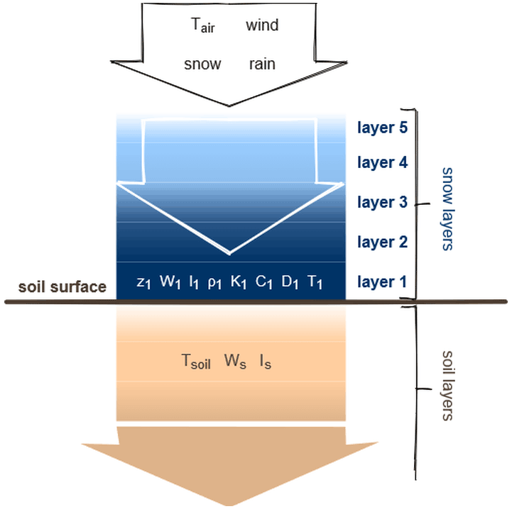
LPJ-GUESS simulates vegetation dynamics on individual and patch scales, taking into account growth, competition for resources, and disturbances. This feature makes it possible to assess how changes in environmental conditions affect vegetation distribution and composition. In this study, we applied 15 plant functional types (PFTs) that characterize arctic ecosystems (see Table S3 in the Supplement). Permafrost dynamics follow Wania et al. (2009) and are simulated using the physical characteristics of 15 soil layers, each 10 cm thick. Soil thermodynamics is governed by climate and snow conditions, and the thermal properties of each soil layer depend on the ice, water, air, mineral, and organic soil fractions. The layer-specific thermal properties define the rate of heat transfer through the soil column. For more details on the model structure, see Smith et al. (2001, 2014), Wania et al. (2009), and references therein. To assess the newly developed intermediate-complexity snow scheme's performance and influence, we conducted simulations with both the old Static and the new Dynamic snow schemes.
2.1 Static snow scheme
The Static snow scheme, which has been in use in LPJ-GUESS until now, treats snow as a single layer with constant values for thermodynamic parameters. Snowfall is simulated on any given day when precipitation (P, mm) occurs and air temperature (Tk, ∘C) is at or below Tmax (∘C) – which is the temperature maximum at which precipitation occurs in snow form. Tk denotes the temperature of a layer k, in this case the air layer. Snow density (ρk, kg m−2) and snow thermal conductivity (Kk, ) are constant at 362 and 0.196, respectively. Snow heat capacity (Ck, ) is calculated by Eq. (1) (Fukusako, 1990).
Compaction processes are not represented in the Static scheme. Snowmelt (melt, mm) is governed by air temperature and precipitation and follows a linear function as shown in Eq. (2) (Choudhury and DiGirolamo, 1998).
The snowpack is homogeneous in its physical properties, and neither internal processes nor seasonal dynamics are simulated using the Static scheme. Using this approach, snow conditions are assumed to be uniform across the Arctic regardless of air temperature regime or seasonal snow dynamics. Due to the heterogeneity in Arctic surface and local climatic conditions, this scheme has a limited ability to represent the variability in high-latitude ecosystems – this is the main shortcoming of the Static snow scheme that this study sets out to improve.
2.2 Dynamic snow scheme
The schematic structure of the multi-layer snow scheme is shown in Fig. 1. The occurrence of snowfall on any given day depends on air temperature and precipitation, using the same principle as for the Static scheme. Fresh snow density (ρfresh, kg m−3) is calculated by taking into account air temperature and wind speed, following Eq. (3), where a, b, and c are scaling parameters defined by Vionnet et al. (2012) (for parameter values see Table A1 in the Appendix).
U10 denotes the 10 m height wind speed (m s−1), following the detailed snowpack model Crocus (Vionnet et al., 2012). To avoid unrealistically low snow density values that may occur in rare cases, the density minimum is set to 100 kg m−3.
The new snow scheme simulates internal snowpack dynamics with up to five snow layers, taking into consideration each layer's depth. Fresh snow either initiates a snowpack or is added to already existing snow layers. If the freshly fallen snow is added to the snowpack, the physical properties of the snow layer are updated. The number and thickness of snow layers are defined according to predefined thresholds: a new snow layer is initialized when an existing layer exceeds twice the prescribed threshold height (2 × 100 mm). If a single snow layer exists but does not reach the minimum height (set to 50 mm), the shallow snow layer properties are combined with the top soil layer. Thereafter, their properties (ice, air, and liquid water fractions and heat capacity) are scaled using weighted averages based on the layer's ice, water, and air fractions for the sake of computational stability. In the case where all five layers exceed the prescribed maximum threshold, the bottom layer accumulates snow in order to preserve and align vertical resolution near the surface of the snowpack. The snow layer density (ρk) and depth (zk, m) relationship is described by Eq. (4), where Ik (kg m−2) defines the ice content of a layer (Lawrence et al., 2019).
The density of a snow layer changes through compaction, which is simulated by two processes: (1) mechanical compaction due to pressure from the overlying snow layers as shown in Eq. (5) (Best et al., 2011).
The increase in the snow layer's density (∂ρk) depends on the mass of overlying layers (Mk, kg). ηk (106 Pa s) denotes the compactive viscosity factor, ks is an empirical constant defined by Best et al. (2011) with a value of 4000 K, and ρ0 is a reference density (50 kg m−2). Snow density may also change by (2) phase changes as a result of freeze–thaw processes within the layers. If a layer's snow or liquid water content changed during freeze–thaw events, its depth and density properties are recalculated, taking into account the snow and ice fractions of the layer as shown in Eq. (4).
In contrast to the Static formulation, phase changes within the snow layers depend on the layer's internal temperature, and this controls the melting process in the Dynamic snow scheme. This development enables the simulation of mid-winter melt events and ensures an improved representation of internal snowpack thermodynamics. Upon melt, each layer can retain a fraction of liquid water based on Eq. (6), where rwmin and rwmax are empirical constants and ρt is a reference density (Wang et al., 2013; Anderson, 1976).
If the liquid water content (Wk, mm) of a layer exceeds the maximum water holding capacity (, mm), water is passed to the layer underneath following a simple bucket model. Rain-on-snow events (ROSs) are simulated if it rains while a snowpack is present. The energy of rainwater may induce phase changes in the snow layers. The overflow liquid water is forwarded to the underlying snow layers and lastly to the top soil layer to percolate to the soil or to be discharged as runoff.
Each layer is characterized thermodynamically by the following physical properties: density, temperature, thermal conductivity, heat capacity, and diffusivity (Dk, m2 d−1). Thermal conductivity is calculated using density as shown in Eq. (7) (Best et al., 2011), following a power function ().
Heat capacity is determined by taking into account snow layer density and temperature according to Eq. (1). The snow diffusivity is calculated by Eq. (8). Soil and snow layer temperatures are computed, taking into account each layer's thermal conductivity, heat capacity, and height, using the Crank–Nicolson finite difference method to solve Eq. (9) (Lawrence et al., 2019).
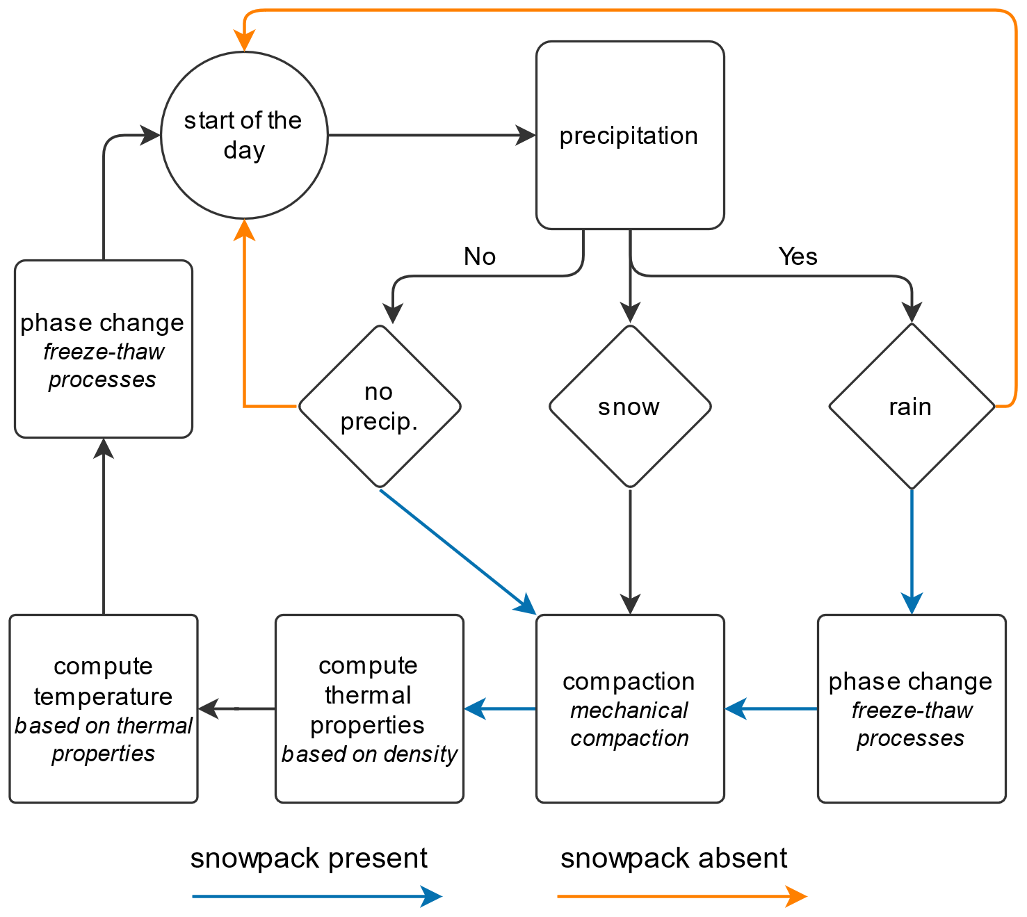
Figure 2Steps in the daily computational cycle for the Dynamic snow scheme. Blue arrows indicate workflow in case a snowpack is present on the ground, while orange arrows show steps when a snowpack is absent.
The computational cycle ends by rearranging the layers based on the depth thresholds, taking into account the potential liquid water content. First we re-calculate each snow layer's depth based on the amount of snow and liquid water using Eq. (4). We then re-arrange the layers by using the leaky-bucket approach, where the snow layers are filled up from the bottom layer (closest to the surface). If the threshold depth is reached, a new snow layer is initiated and the process continues until the total depth of the snowpack is distributed to the specific snow layers. The overflow meltwater is passed to the soil for percolation after this step. This cycle is repeated each day when there is a snow or rain-on-snow event. The daily snow cycle of the Dynamic snow scheme is depicted in Fig. 2.
Besides the changes in the representation of snow, the calculation of heterotrophic respiration below 0 ∘C was changed following a recent data synthesis (Natali et al., 2019) to better represent arctic conditions. This adjustment was implemented for both the Static and Dynamic schemes. The minimum decomposition temperature was set to −20 ∘C, and the Q10 value was set to 2.9. A comparison between the old and new functions is shown in the Supplement (Fig. S1 in the Supplement). This adjustment led to higher soil respiration in both schemes during the cold season compared to the old model set-up.
The implemented processes and physical representations are simpler than in dedicated, high-resolution snow models – such as Crocus and SNOWPACK (Lehning et al., 2002; Vionnet et al., 2012) – but reflect the model improvements identified as being most important in previous model inter-comparison studies (Krinner et al., 2018). These improvements enable us to simulate a more realistic range of snow conditions and soil thermal conditions across the Arctic.
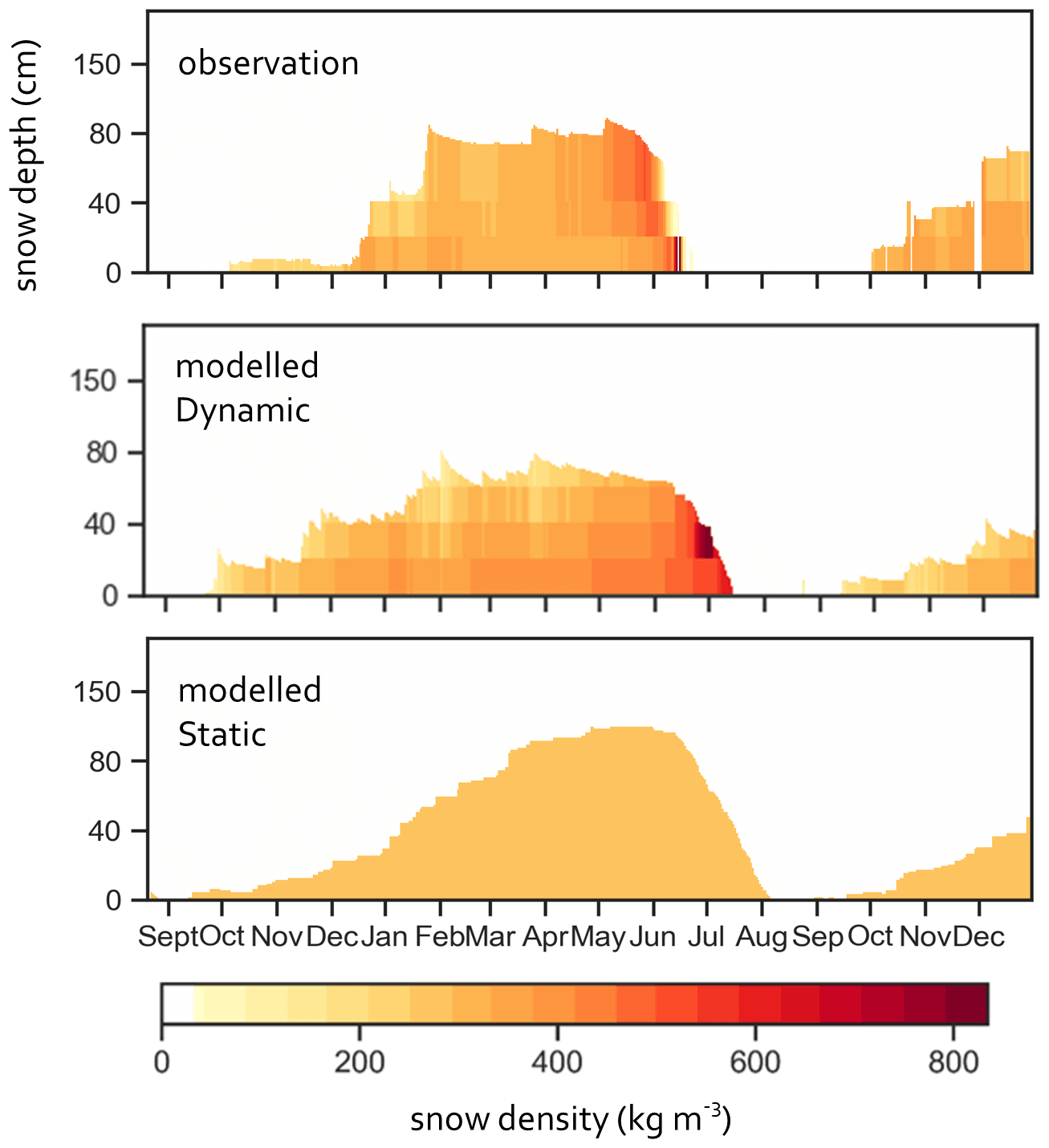
Figure 3Snowpack dynamics at the Zackenberg GeoBasis station. Density values for the layers are extrapolated – from three and five layers for the observational and modelled data, respectively. The colours of the snowpack indicate snow density.
2.3 Simulation set-up
The performance of LPJ-GUESS using both snow schemes was compared at the site and regional levels. Modelled properties were compared to observational datasets, when available. We quantified the correspondence between simulated and measured variables using statistical methods.
- i.
Site-level comparison.
To highlight the differences in snowpack dynamics using the two snow schemes, we compiled a detailed single-site model–data comparison of the internal snowpack structure (Fig. 3). Afterwards, we ran the model for five well-studied northern high-latitude sites in order to identify how well the two snow schemes can simulate snow and soil temperature at the site level. These sites are Abisko, Zackenberg, Bayelva, Kytalyk, and Samoylov – see site details in Table S1 in the Supplement. Measurements of snow depth and soil temperature were sorted and averaged on a daily basis – 10 years for the simulations and all available years for observations at each site. Model outputs were examined and compared to these time series to evaluate the snow schemes' ability to simulate snow depth and soil temperature seasonality adequately.
- ii.
Regional simulations.
We conducted simulations for a set of Russian sites (256 sites) which were part of the study by Wang et al. (2016), as a follow-up, and re-evaluate the snow insulation effect in LPJ-GUESS over a large region. First, snow depth and soil temperature data were sorted monthly for each site for the years 1980–2000. Site observations were provided by the All-Russian Research Institute of Hydrometeorological Information – World Data Centre (RIHMI-WDC; http://meteo.ru/, last access: 3 January 2019). Following this, averages were calculated for December, January, and February. The difference between soil (25 cm depth) and air temperature – henceforth ΔT – was used as a proxy to evaluate the strength of the model-simulated insulation effect. Snow depth, soil temperature, and ΔT series were grouped according to air temperature to evaluate the insulation capacity under different temperature regimes.
- iii.
Pan-Arctic simulations.
Finally, we conducted model simulations across the Arctic to assess the effect of changing the snow scheme on selected physical and biogeochemical variables and vegetation properties. When applicable, variables were averaged over December, January, and February to emphasize the effect on the winter season. Instead of the absolute results, we show the difference between the set of simulations, calculated as the difference between Dynamic and Static model outputs.
3.1 Site-level simulations
Prior to the evaluation of the large-scale performance of the new Dynamic snow scheme, we conducted a single-site comparison to examine the validity of the results. These detailed snowpack observations from Zackenberg helped to determine whether the Dynamic scheme can simulate internal snowpack dynamics, snow depth, and snow density.
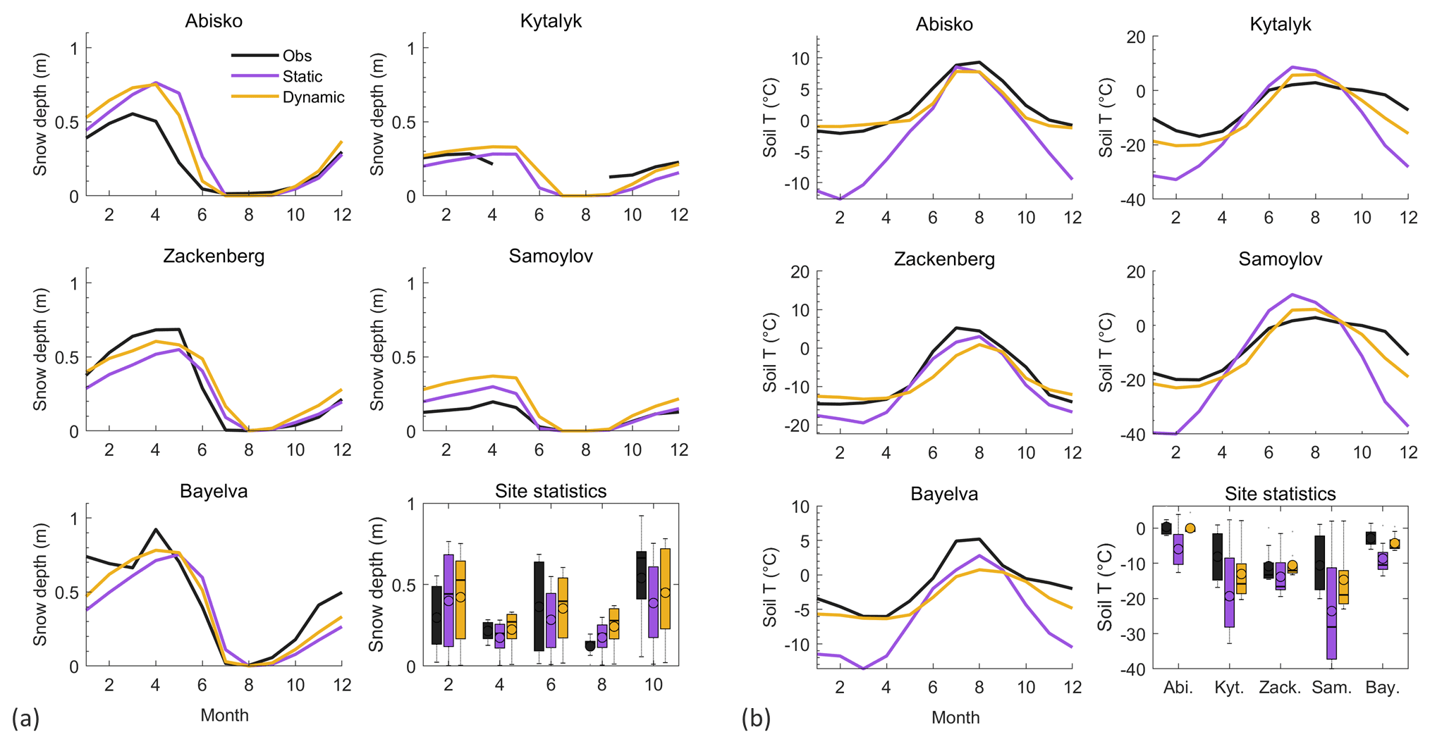
Figure 4Seasonal cycle of (a) snow depth and (b) soil temperature at 25 cm depth for the studied sites, comparing model simulations and observations. Site statistics show the spread of monthly snow depth and soil temperature values for the respective sites – excluding the summer months (June–July–August).
We established the ability of the new snow scheme to simulate snow conditions by comparing a simulated snowpack with snow depth and density observations from Zackenberg (2013–2014 snow season). Figure 3 presents the observed and simulated snowpack by the Dynamic and Static schemes. This figure shows that the Dynamic scheme simulates comparable snow depth and that the simulated snow densities follow the observed snow density pattern through the snow season. Density values are compared qualitatively, since it is difficult to accurately align the observational and modelled layer densities. To be consequent, we used global climatic forcing data for all simulations in this study, including this site-scale comparison. This fact should be taken into account when interpreting the model–data comparison in this section – as some of the differences may be derived from the differences in climatic data.
There are lower densities early in the snow season, with fresh snow having low density, while density increases in late spring, during the melt season. The Static scheme with constant snow density simulated a somewhat higher-than-observed snow depth. Thermal properties in snow layers are derived from density, and this is especially important in the Dynamic snow scheme. Dynamically simulated density translates to more realistic thermal conductivity dynamics, which governs the rate of heat transfer through the snowpack. This feature is essential in simulating a reliable atmosphere–snow–soil heat transfer interaction. The difference in snow depth between the Static and Dynamic simulations is most visible at the end of the snow season, before the start of snowmelt – as indicated in Fig. 3, bottom panel.
Overall, the new scheme reproduces the snow dynamics over the cold season better than the Static scheme. Taken together, these results suggest that the Dynamic scheme is skilled in simulating the snowpack's internal structure and dynamics. Since the Static scheme has a constant snow density throughout the snow season, the Dynamic scheme is expected to better capture the seasonal behaviour of snow and soil conditions. The Zackenberg site comparison indicated that the Dynamic scheme successfully integrated these key processes affecting the density over the snow season. In this study, we used a global climate forcing dataset, which may explain some of the observed model–observation differences. The mismatch between snow observations and simulations is influenced by the use of the global model forcing dataset instead of site-specific temperature, precipitation, or snowfall time series.
Table 1RMSE for soil temperature and snow depth for the applied snow schemes for the single site simulations.
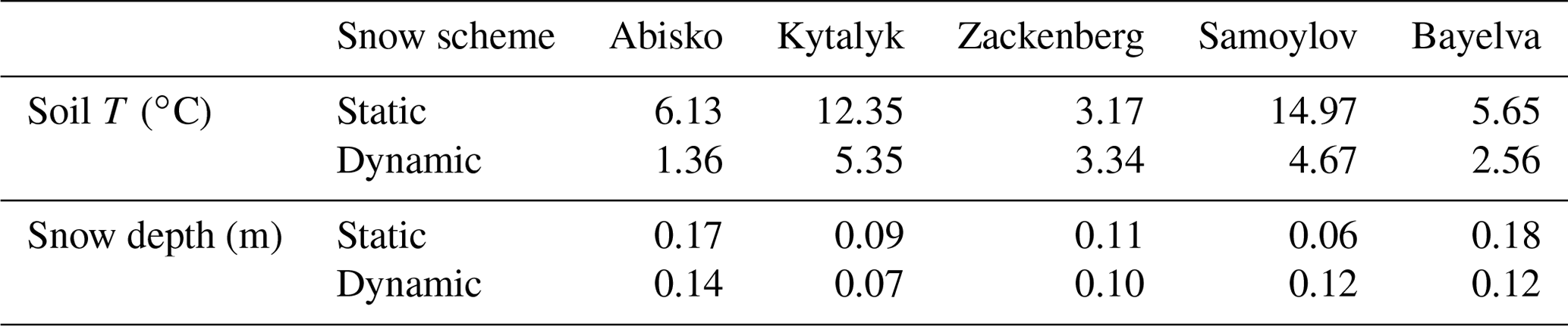
We moved to a multi-site analysis to compare the Static and Dynamic snow schemes on five well-documented sites. To assess the performance of the two snow schemes, we composed seasonal cycles based on monthly averages of (a) snow depth and (b) soil temperature at 25 cm depth, shown in Fig. 4. The corresponding root-mean-squared error (RMSE) for each study site is shown in Table 1. Generally, the Dynamic scheme shows only minor improvements in the simulation of snow depth. Despite this, modelled soil temperatures are much closer to the observed values for all sites, especially during the winter months. This behaviour highlights that changing the internal snowpack dynamics with the Dynamic snow scheme had a significant effect on soil temperature, even when the simulated snow depth differed marginally. The changes in soil temperature are due to the differences in snow thermal properties, which significantly influenced the insulation capacity of the snowpack.
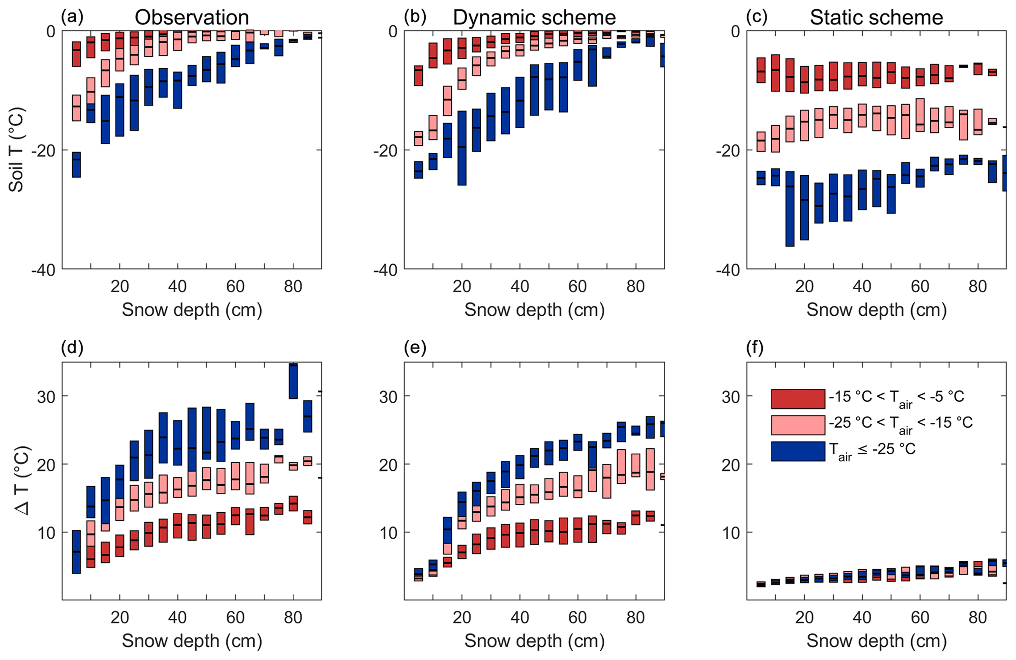
Figure 5Comparison of the observed and modelled snow insulation effect at the Russian sites between observations and model simulations using the Dynamic and Static schemes. (a–c) Soil temperature and snow depth relationship. (d–f) Difference in air–soil temperature and snow depth relationship. Snow depth presented on the horizontal axis is classified in 5 cm depth bins. Colours indicate different air temperature regimes, and upper and lower bars show the 25th and 75th percentiles.
The implementation of the new snow scheme resulted in significant changes within the snowpack that are responsible for the improved soil temperature simulation. The Static scheme applies constant snow density and thermal conductivity, which defines the rate of heat transfer through the snowpack. In the Dynamic scheme, thermal conductivity is dependent on the dynamically updated density; therefore the new scheme can achieve a more realistic simulation of snow heat transfer dynamics throughout the snow season – depending on environmental conditions. The Dynamic scheme simulates snow thermal conductivity in a range from 0.04 to 0.5 , which aligns well with literature estimates of 0.021–0.65 . This feature enables the simulation of a wide range of conditions across the Arctic, as opposed to the general conditions assumed by the Static scheme.
The statistical comparison (site statistics) shows that there is a smaller variance of modelled values of soil temperature using the Dynamic snow scheme, which indicates an improvement in comparison to the Static simulations' outputs. The RMSE (Table 1) also shows that the Dynamic scheme provides an improved fit of simulated soil temperature and snow depth at most sites. Overall, we conclude that, with the Dynamic scheme, the model is able to simulate snow and soil temperatures that correspond better with the observed ranges.
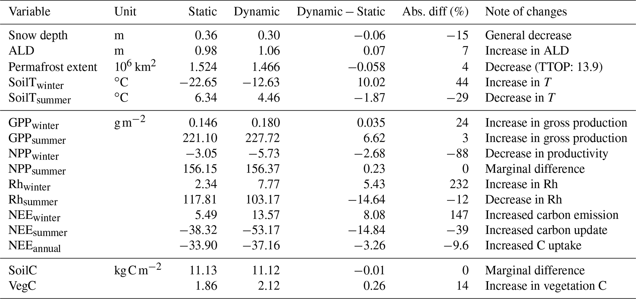
Table 2Pan-arctic mean values for the studied variables for the Static and Dynamic simulations and their respective differences.
3.2 Russian site simulations
Following the Dynamic scheme's improved performance at the site level, we further evaluate the model's performance at the regional scale for the same sites as in the previous model intercomparison by Wang et al. (2016) that highlighted shortcomings in the snow scheme of LPJ-GUESS. Figure 5 shows the snow insulation effect over a set of Russian sites, using the two snow schemes, where the coloured bars show different temperature regimes. The figure is compiled from 20 winter season average values of near-surface soil temperature (25 cm depth) and snow depth per site. Due to the air-temperature-based classification, the number of samples per bin is not balanced, which led to an uneven number of values allocated to the different groups. The top row of Fig. 5 shows that the Dynamic snow scheme has better skill in simulating the relationship between soil temperature and snow depth than the Static scheme. It must be noted that there is a clear difference between the current Static scheme simulations and results reported by Wang et al. (2016), which is due to recent updates in the model, independent of the snow module, and the different climate forcing dataset used in this study.
It is apparent from the ΔT and snow depth relationship (Fig. 5, bottom row) that the Dynamic scheme reproduces the observed insulation effect well. Unlike the Static scheme, the new snow module can also simulate the different insulation behaviour depending on the air temperature regimes. The improved performance of the Dynamic scheme is confirmed by the root-mean-squared error (RMSE), shown in the Supplement (Table S2 in the Supplement). RMSE decreased significantly for both the soil temperature–snow depth and ΔT–snow depth relationships. This regional analysis confirmed that the new Dynamic snow scheme has an improved skill in simulating winter soil conditions.
3.3 Pan-Arctic simulations
To assess how the two snow schemes differ in simulating seasonal snow across the Arctic, we subtracted output variables from simulations with the Static module from those with the Dynamic module. We calculated average conditions for winter (December–January–February) and summer (June–July–August) for the period 1990–2015. The mean pan-arctic seasonal dynamics of snow depth, soil temperature, and upper soil water content are shown in the Table 2.
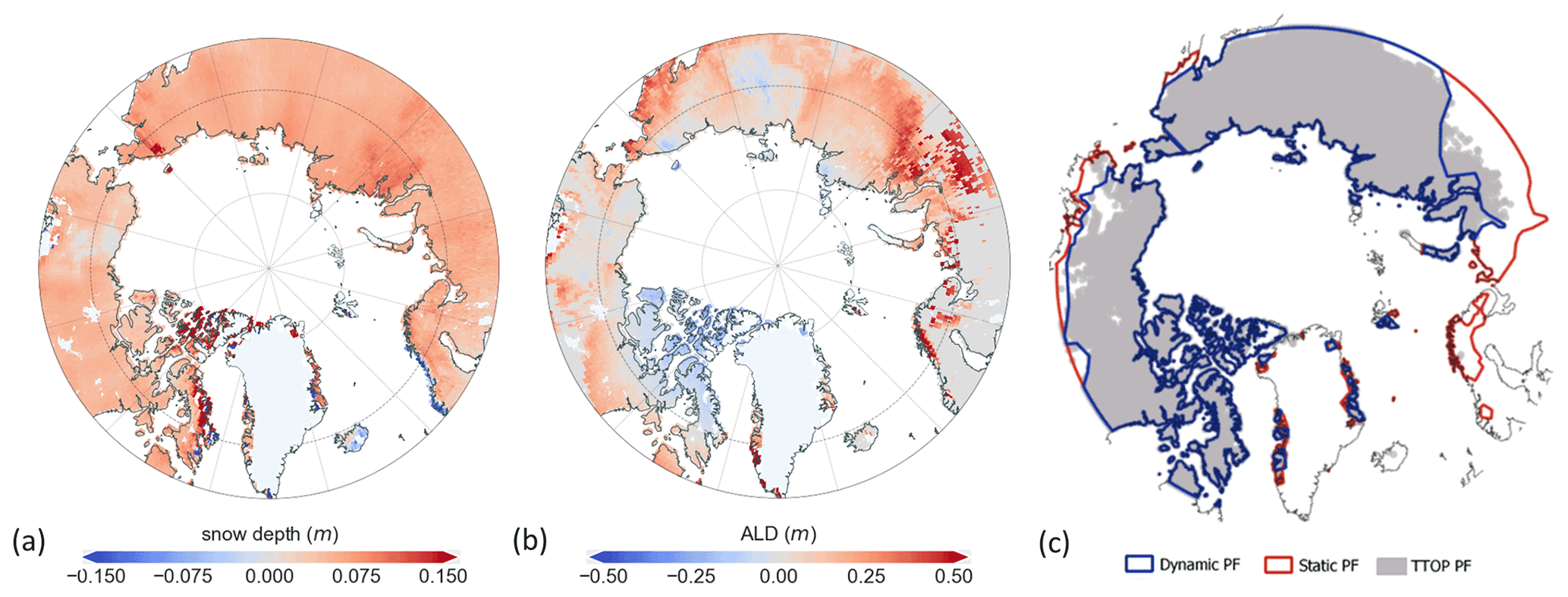
Figure 6(a) Snow depth difference in winter months and (b) maximum ALD difference, calculated by subtracting the Static from Dynamic simulation outputs. Modelled permafrost extent is based on mean annual ground temperature (MAGT) and plotted against the permafrost cover estimate by Obu et al. (2019a) (TTOP model). Simulated absolute snow depth is shown in Fig. S2 in the Supplement and ALD in Fig. S3 in the Supplement.
3.3.1 Impacts on physical variables
Figure 6a shows the difference in simulated wintertime snow depth. The Dynamic scheme shows an overall lower snow depth across the Arctic with the most pronounced changes in coastal Norway and in western Siberia. On average, the snow depth for the Dynamic scheme is 6 cm lower due to the implementation of snow-related processes affecting snow density and consequently snow depth.
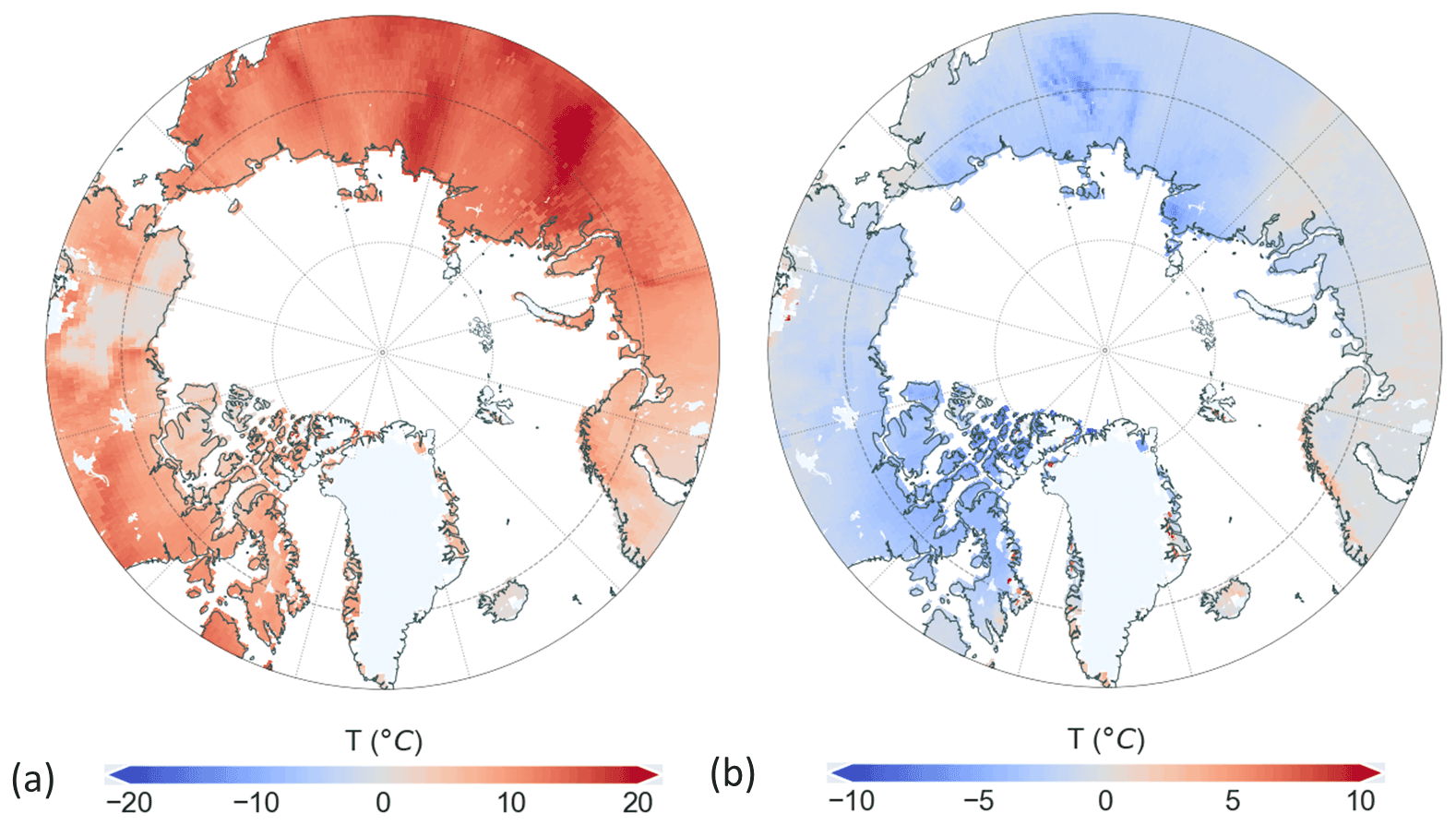
Figure 7Near-surface soil temperature (25 cm depth) difference between the Dynamic and Static simulations, for winter (a) and summer (b) seasons. Differences are calculated by subtracting the Static from Dynamic simulation outputs. The absolute simulated soil temperatures using the two snow schemes are shown in the Supplement in Fig. S4.
The main aim of developing the new snow scheme was not only to enhance the simulation of snow depth but also to improve the simulation of snowpack properties that directly affect soil conditions. Therefore, we investigated how the internal structural changes in the representation of snow influenced soil temperatures. The soil temperature differences shown in Fig. 7 reveal that the new snow scheme influenced the winter season to a large degree, both within and especially outside of the permafrost region. Winter soil temperatures are higher with the Dynamic scheme, while it results in a cooler near-surface soil temperature during the summer. A closer look at the monthly soil temperature values in Fig. 11 showed that spring months are cooler for the Dynamic scheme but that the difference between the two schemes decreases towards the end of summer. This pattern is more pronounced in the permafrost-underlain regions. This shows that the Static snow scheme has too little insulation and results in soil temperatures that are too cold during the winter months, as we also show in the site simulations. Moreover, the Static scheme also does not insulate soils sufficiently during the springtime when air temperatures rise above 0 ∘C, which allows the soil to warm up more quickly even in the presence of a snowpack.
The depth to which the top soil thaws during summer, and refreezes in winter, in permafrost areas is called the active layer depth (ALD). The difference in the seasonal maximum active layer depth for the model simulations is shown in Fig. 6b. Since the Dynamic scheme had warmer soil temperatures, the modelled permafrost extent is smaller than with the Static scheme. We compared our model simulations with a recent satellite-driven permafrost extent estimate by Obu et al. (2019a) – from here on referred to as the TTOP model. Modelled permafrost extent was defined by the area where the mean annual ground temperature (25 cm depth) was below zero. The Dynamic scheme's permafrost extent is much closer to the TTOP model's estimate, while the Static scheme simulates a much larger permafrost extent, as shown in Fig. 6c. The Dynamic scheme's computed areal permafrost cover, while improved compared to the Static scheme, still overestimates the TTOP model estimates by approximately 5 % (see Table 2).
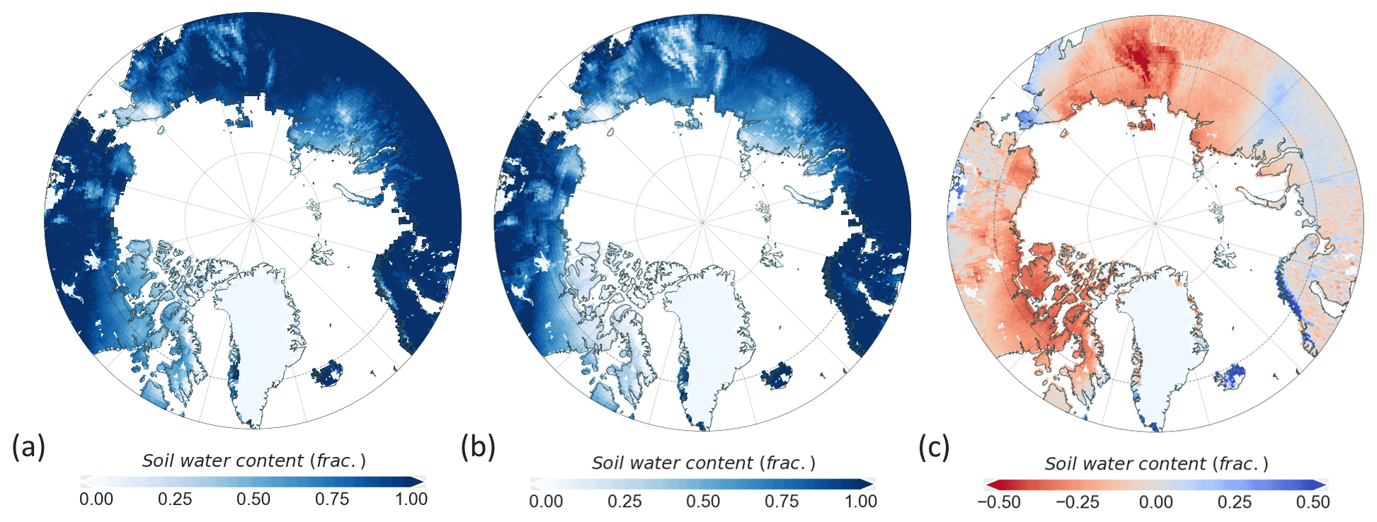
Figure 8Mean fractional water content of the upper soil column in May, June, and July, using the Static (a) and Dynamic (b) schemes and their difference (c). Differences are calculated by subtracting the Static from Dynamic simulation outputs.
Besides governing the physical state of permafrost, snow and soil temperature also have a large influence on the temporal and spatial patterns of soil water content. We show the simulated upper soil column water content in Fig. 8. This figure shows the mean fractional soil water content over May–June–July. Soil water content was calculated using the average seasonal liquid water content from the top 50 cm of the soil column. Soil water content is represented as the fraction of the available capacity between the wilting point and field capacity, and therefore frozen water is not included in these values. Figure 8c shows that there is a higher water availability within the permafrost region using the Static scheme. Water availability is a key driver of the start of the growing season, nutrient availability, and vegetation dynamics. The time-series analysis of upper soil water content highlights that the snowmelt rate is not significantly different between the schemes. Still, there is a large difference in soil temperature dynamics. The Static scheme's soil temperature increases more rapidly during the spring than the Dynamic scheme's soil temperature (see Fig. 11a and b). This results in an earlier onset of snowmelt and earlier increase in soil water availability and nitrogen mineralization. This affects productivity, which we assess in the coming sections. Although the difference in water content and nitrogen mineralization between the snow schemes converges towards zero as summer progresses, we show that the change in snow scheme had a lasting effect beyond the cold season.
Overall, the new snow scheme had a substantial effect on winter soil temperatures. As a result, summer conditions were also altered by the snow scheme updates. It is apparent that the largest changes in snow depth and temperature coincide. For instance, along the Norwegian coast and in central Siberia. Taken together, our results show that the Dynamic snow scheme improved the simulation of physical variables.
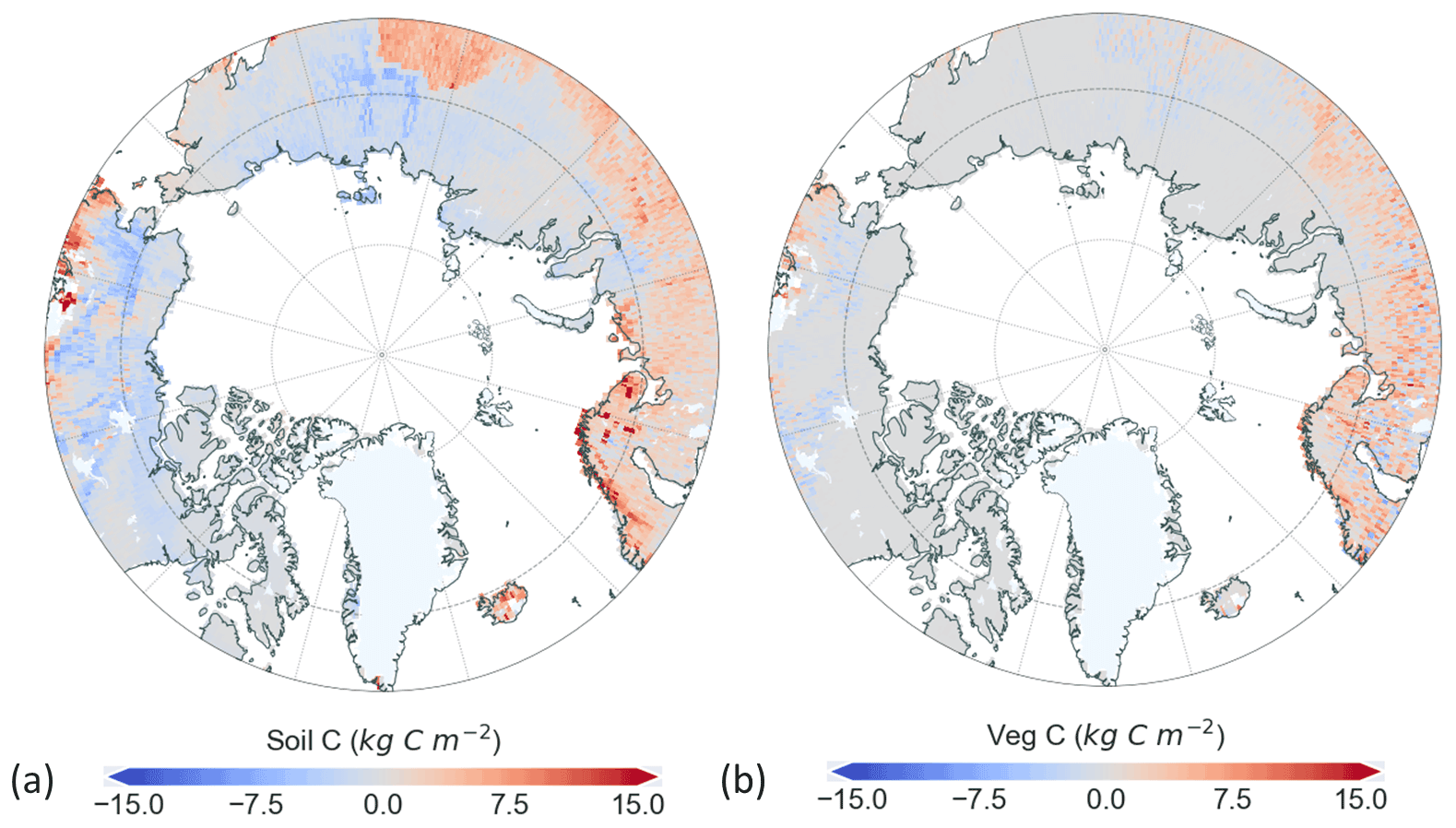
Figure 9The difference in simulated soil (a) and vegetation carbon pools (b) between the two schemes. Differences are calculated by subtracting the Static from Dynamic simulation outputs.
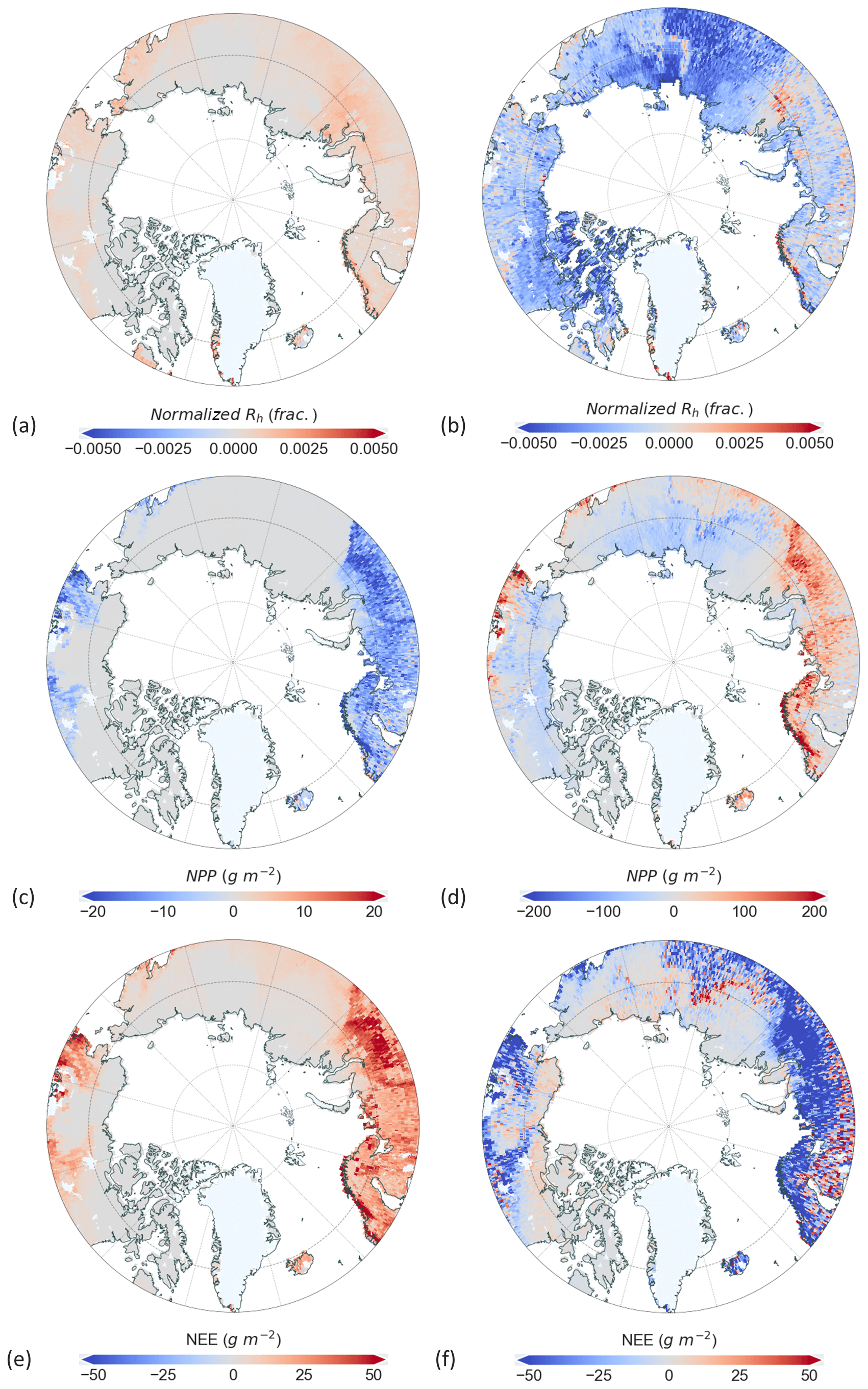
Figure 10The difference in normalized heterotrophic respiration for winter (a) and summer (b) between the two schemes. Differences between simulated Dynamic and Static winter (c) and summer (d) NPP. Differences between simulated Dynamic and Static winter (e) and summer (f) NEE. Differences are calculated by subtracting the Static from Dynamic simulation outputs. Simulations for the two schemes are shown in Figs. S5 (heterotrophic respiration), S6 (NPP), and S7 (NEE) in the Supplement.
3.3.2 Impacts on biogeochemical variables
Besides the impact on soil thermodynamics, we investigated how key biogeochemical components – such as productivity and carbon pools – were affected. The changes across seasons and permafrost conditions are summarized in Figs. 11 and 12.
Our simulated soil carbon pools (Fig. S6 in the Supplement) deviate from literature values (Hugelius et al., 2014) and are consistently lower across the Arctic. The main reason for this is the model's representation of soil organic matter processes. Soil carbon and nitrogen are represented by pools that exist in the top 50 cm of the soil column (Smith et al., 2014) and are thus only influenced by near-surface conditions. Moreover, peatlands are not explicitly represented. The differences in soil carbon between the schemes, as shown in Fig. 9a, coincide spatially with the highest differences in soil temperature. This suggests that the changes in soil temperature influence soil carbon in the model and therefore the rate of respiration from soils as well. Vegetation carbon pools (Fig. 9b) are higher in the non-permafrost region using the Dynamic snow scheme (see Table 2 for mean values). Since the evaluation of soil carbon is not the focus of this study, soil carbon outputs were used to normalize the heterotrophic respiration to be able to interpret the relative differences between schemes (Fig. 10a and b). To do so, we divided the heterotrophic respiration by the soil carbon estimates for the respective simulations using the two snow schemes. With the Dynamic scheme, summer soil respiration decreased across the Arctic. Winter respiration, on the other hand, increased, except for in eastern Siberia. These changes in soil respiration can be attributed to changes in soil temperature, as shown in Fig. 7.
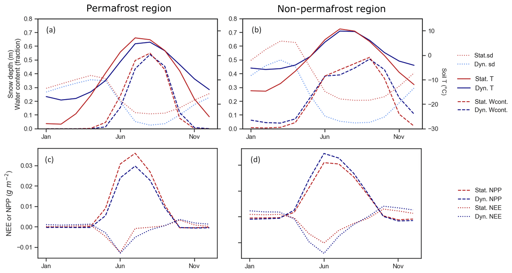
Figure 11Seasonal dynamics of snow depth, soil temperature (25 cm depth), and fractional soil water content within (a) and outside of the permafrost region (b). Seasonal dynamics of NEE and NPP within (c) and outside of the permafrost region (d).
The difference in net primary productivity (NPP) between simulations with the two snow schemes for both winter and summer is shown in Fig. 10c and d, where positive NPP means more carbon uptake by the vegetation. We note an impact of the different snow schemes on summer productivity, caused by the different soil thermodynamics and soil water availability during the spring and early summer period. This artefact is also visible in the simulated pan-Arctic NEE, in Fig. 10e and f, where negative NEE values indicate a stronger uptake of carbon by ecosystems. The positive difference in winter NEE (e) shows that there is a higher carbon release in the winter season for the Dynamic scheme in central Europe, western Siberia, and coastal Norway. The mean winter NEE of the Dynamic scheme more than doubled (Table 2). Compared to the Static scheme, which relates to both the change in soil respiration and NPP. Figure 11c and d show some interesting contrasts regarding the seasonal carbon fluxes. Permafrost-underlain regions (Fig. 10c) experience little difference in the simulated NEE. The Dynamic scheme simulates lower peak summer NPP. Winter NEE in the non-permafrost region is higher using the Dynamic scheme, indicating a larger carbon uptake by the vegetation. On the other hand, we can observe an increased sink capacity (more negative NEE) during the summer months.
3.3.3 Vegetation composition and distribution
Vegetation composition and distribution depend on the changes in physical and biochemical variables described in the previous section. Therefore, we investigated how the application of the two snow schemes affected vegetation distribution to determine if there are shifts in dominant plant functional types (PFTs) as a result of using different snow schemes. The dominant PFT for each simulated grid cell was determined by selecting the PFT with the highest maximum leaf area index (LAI) during the simulation years (1990–2015). Using the Dynamic snow scheme, roughly half of the sites are dominated by summergreen low shrubs and boreal needle-leaved evergreen trees (LSS with 25 % and BNE with 23 %; see Table S3). Prostrate dwarf shrubs, (SPDS), graminoid and forb tundra (GRT), and boreal needle-leaved summergreen trees (BNS) accounted for 20 %, 8 %, and 7 % dominance, respectively. For an easier comparison between the Static and Dynamic simulations, PFT classes were grouped into forest, open grass, shrubs, and no vegetation categories after determining the dominant PFT in each grid cell (classification based on Wolf et al., 2008). This classification showed that grassland classes dominate (56 %), followed by forest cover (36 %). Shrubs dominate at 29 % of the simulation sites. There is a negligible number of sites with mostly bare soil. When comparing the spatial pattern of dominant vegetation groups, we noted that there is only a marginal difference between the Static and Dynamic simulations (see Fig. S10 in the Supplement). Changes in group dominance between the Static and Dynamic simulations occurred at approximately 10 % of the sites; see Fig. S11 in the Supplement. The Sankey diagram shows the direction of change between the three groups. Myers-Smith et al. (2011) suggest that increased soil temperature leads to a shift to an increased forest height and shrub cover. Grass-to-shrub domination change (3.1 %) was the most prevailing change, which indeed points towards an increase in vegetation height. However, we observe a shrub-to-grass (1.95 %) shift in domination at the same time; therefore, we cannot conclude the main direction of changes.
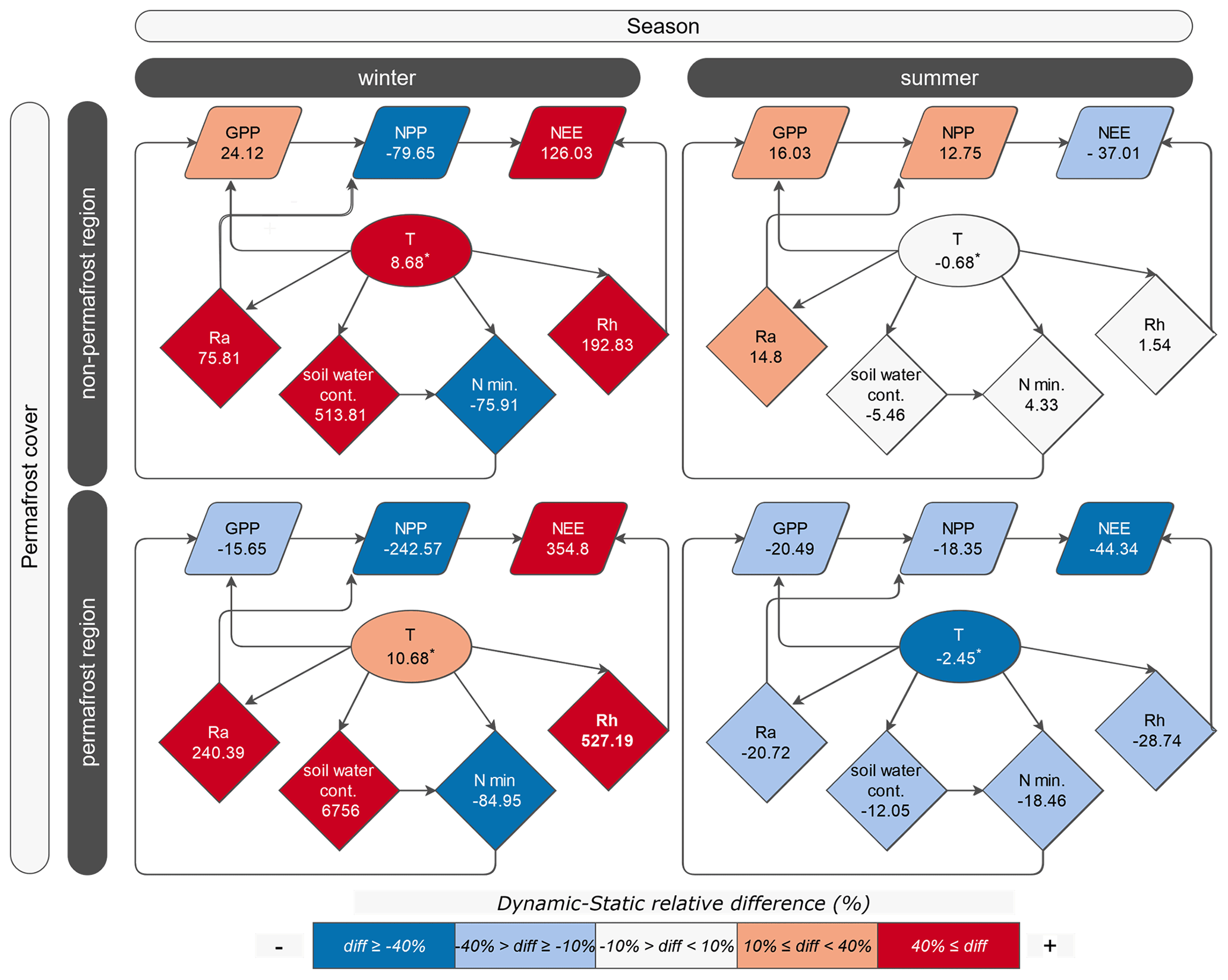
Figure 12Relationship between variables during the winter and summer seasons, within and outside of the permafrost region. The colour of the boxes indicates the direction and qualitative magnitude of changes in the variables, based on the relative difference (%) between Dynamic and Static schemes – shown in the boxes below the variables. Variables are shown as follows: GPP: gross primary production (g m−2); NPP: net primary productivity (g m−2); NEE: net ecosystem exchange (g m−2); Ra: autotrophic respiration (g m−2); Rh: heterotrophic respiration (g m−2); Nmin: net nitrogen mineralization (kg N ha−1); soil water content: fraction. The relative changes in soil water content (in %) are high in the winter due to the low fractional water content values as we only account for the liquid soil water and do not consider the amount of frozen water in the soil. These changes correspond to small absolute changes in fractional soil water content. ∗ Note: temperature differences are shown as absolute differences for easier readability.
3.4 Cause-and-effect relationships
As many of the reviewed processes interact with each other in a complex, non-linear manner, change in one variable may not translate to a direct impact on another variable. To provide an overview of our findings regarding the physical and biogeochemical processes, we created a flow chart showing observed changes in modelled state variables and their connections. Figure 12 shows the difference between simulations using the two snow schemes – calculated by subtracting the Static from Dynamic results. Reddish box colours show that the Dynamic scheme had higher values, and blueish colours show that the Dynamic scheme simulated lower values than the Static scheme. The lightness and darkness of the colours indicate the magnitude of changes between the winter and summer seasons qualitatively.
Each box contains the computed difference, and Table 2 summarizes the mean changes in these key variables. Considering the spatial pattern across the Arctic, we conclude that the pattern of changes and differences between the Static and Dynamic simulations vary depending on the presence or absence of permafrost cover. For a more detailed evaluation, process relationships are therefore divided into permafrost and non-permafrost regions. Since snow depth only affects these variables indirectly, through insulation, it was not included in the feedback graph. The choice of snow scheme induced changes in near-surface temperature (T), which is the key governing factor over these variables. In general, higher soil temperatures during the winter season prompt a positive response in respiration, soil water content, and vegetation primary productivity. Soil temperature increased to a greater degree in the non-permafrost region during the winter season. The same increasing pattern is observed for heterotrophic (Rh) and autotrophic respiration (Ra), soil water content, and NEE. Nitrogen mineralization decreased in the wintertime, with a larger decrease outside of the permafrost region. In contrast, summer months' average soil temperature showed an overall decrease in the permafrost region. This is due to the different thermal soil and snow dynamics in the two applied snow schemes. We observed rapid heat loss using the Static scheme, resulting in insufficient insulation during the snow season. The same feature causes soil temperature to rise rapidly in the spring, when air temperature is already above zero but a snow cover remains present. Faster soil warming leads to increased soil water availability that affects productivity. Respiration and NEE are slightly reduced for both permafrost and non-permafrost regions in the Dynamic scheme during the summer. Differences noted for the summer are smaller for all variables than in the winter season.
4.1 Snow scheme dynamics
The site-level analysis shows that the new Dynamic scheme is able to simulate snow height and density adequately due to the implementation of physical processes and a dynamic representation of snow properties. The integrated mechanistic compaction scheme and phase changes within snow layers make it possible to simulate heterogeneous snow density and thermal properties within the snowpack. This influences the simulated snow density directly by altering snowpack structure. Density regulates heat transport rate through snow layers by affecting thermal conductivity (Eq. 7): lower density results in a more insulating cover, whereas higher density and compacted layers are a better heat-transferring medium and exhibit lower insulation. In the Static scheme, snow density was assumed constant through the snow season and across all study sites. Such static snow representation is unsatisfactory when simulating arctic conditions (Krinner et al., 2018). The new snow scheme provides an improved framework for a mechanistic snow season simulation.
The single site simulations (Sect. 3.1) provide reasonably consistent evidence that the new snow scheme's implementation leads to significant changes in near-surface temperature simulation – especially at Abisko, Bayelva, and Samoylov. As shown by Chadburn et al. (2017), the site-wise model–data comparison is challenging since point measurements may not be representative of a larger area due to the complexity in topography and vegetation conditions. The model–observation fit may be improved by using site-specific climatic forcing instead of a global gridded dataset.
To avoid site-specific problems in the interpretation of simulations, we also evaluated the model at a regional scale. By comparing the results of the Russian site simulations (Sect. 3.2) with those of Wang et al. (2016), we conclude that the development of the representation of snow in LPJ-GUESS significantly improved air–soil temperature and snow depth–soil temperature relationships. The Dynamic snow scheme's insulation capacity followed a quasi asymptotic trend, increasing with snow depth and slightly levelling out after reaching the so-called effective depth at 30–40 cm (Slater et al., 2017). The insulation capacity was, in general, slightly lower than observations, with a notable underestimation when snow depth is below 20 cm. Nonetheless, these results are a vast improvement over the old Static scheme, as shown in Fig. 5.
The RMSE values (Table S2) also show that the Dynamic scheme better captured the observed the soil temperature and snow depth relationship than the Static scheme. RMSE was slightly higher for the coldest air temperature regime for both snow schemes. We note that the Static schemes' performance differs from what was shown in Wang et al. (2016). The reasons for these differences are developments of the model since then in components other than the snow scheme and also the different meteorological forcing used in this study. Our results indicate that the enhancement of snow-related processes improves the simulation of soil temperatures in LPJ-GUESS and that the model can be more reliably applied to assess the impact of environmental changes on the arctic carbon cycle.
4.2 Impact on physical and biogeochemical variables
The changes to the snow insulation capacity in the Dynamic scheme had a significant effect on permafrost conditions. Our pan-Arctic results showed that the Static scheme simulated near-surface soil temperatures that were too cold in winter and too warm in summer. Permafrost extent simulated with the Dynamic scheme agreed more closely with the permafrost estimate by Obu et al. (2019a), as shown in Fig. 6. Comparison of these findings with other studies where a new snow scheme was introduced reiterates that the model representation of snow strongly affects soil temperatures (Gouttevin et al., 2012; Wang et al., 2013). Reliable soil temperature simulations are essential to study the permafrost–climate feedback. Biskaborn et al. (2019) concluded that recent warming trends of permafrost soils are partly due to an increase in snow insulation, accelerating its degradation. Both field observations and modelling studies have identified this close link between snow and permafrost conditions (Johansson et al., 2013; McGuire et al., 2016; Lawrence and Slater, 2010). Identifying changes in permafrost-underlain areas is important because of the potential increase in organic matter decomposition and release of greenhouse gases. These aspects will be further evaluated in LPJ-GUESS with the new snow scheme.
We observed a general decrease in mean NPP during the winter and a marginal difference in the summer. Considering the presence of permafrost, however, we noted an increase in GPP and NPP for non-permafrost-underlain areas in summer. The significantly warmer winter soil conditions for the Dynamic scheme caused an increase in heterotrophic respiration – i.e due to faster litter decomposition rates and increased microbial activity. Accordingly, soil respiration increased during the winter in the non-permafrost region. During the summer, there is an overall minor decrease in soil respiration due to the lower soil temperatures simulated by the Dynamic scheme. The net effect of the above-discussed processes is an overall increase in carbon emissions during the winter and an increased uptake during the summer.
The impact of the new snow scheme on summer conditions was surprising. These differences were caused by the changes in spring snow and soil temperatures and soil water availability. During springtime, soils with the Static scheme warm more quickly, due to the lower insulation, which leads to an earlier thaw and increased soil water availability. The Dynamic scheme simulates a more realistic atmosphere–snow–soil heat transfer, leading to a slower temperature transition. The difference between the schemes diminishes towards the end of the summer. Overall, the simulated pan-arctic carbon fluxes are systematically lower than other published values (Efren et al., 2019; Rawlins et al., 2015; McGuire et al., 2012). Virkkala et al. (2021) estimate an annual NEE in the range of −46 to +10 , while our simulations have a mean estimate around −35.5 (see Table 2).
Besides the carbon fluxes, we also evaluated the simulated annual soil and vegetation carbon pools. Vegetation pools were more different when applying the Dynamic, while no clear differences were apparent for soil carbon (see Table 2). With the Dynamic snow scheme, the soil carbon pool is lower within the permafrost region and higher outside of the permafrost region. These results align well with the sensitivity study by Gouttevin et al. (2012), which highlighted that decreased soil carbon stocks can be attributed to a higher respiration rate and increased microbial decomposition rates.
The mean simulated soil carbon content was around 10 kg C m−2, which is much lower than the 50–100 kg C m−2 range suggested in literature (Hugelius et al., 2014; Hugelius, 2012). This difference is most likely due to the fact that we only simulated grid cells with upland soils, while peatlands were not represented. The inclusion of peatlands would have led to a larger amount of soil carbon, since these ecosystems are characterized by waterlogged soils in which decomposition is suppressed – although carbon can be released as methane. Also, all organic matter is considered to be in the top 0.5 m of the soil in the current version of LPJ-GUESS and is therefore only affected by the average soil temperature and moisture conditions down to 0.5 m, but not by conditions further down. These aspects will be taken into account in ongoing model development. Our analysis highlights that the observed differences between the Static and Dynamic schemes correlate well with the spatial pattern of near-surface soil temperature changes. This shows that the changes in soil temperature influence the soil carbon content in the model. The shortcomings in soil carbon simulation will be addressed and improved in the future, which will enable a more reliable carbon pool assessment.
4.3 Impact on vegetation dynamics
Satellite-based studies have identified an overall greening trend across the Arctic, in response to a warming from the 1980s until now. However, they also showed that this greening trend is not uniform and certain areas have actually experienced browning (loss of greenness) during this period (Berner et al., 2020; Myers-Smith et al., 2020). This may be partly due to damage to vegetation following extreme winter events (Phoenix and Bjerke, 2016). At the site level, a recent study by Niittynen et al. (2020) showed that winter thermal conditions are a strong control on vegetation patterns in arctic landscapes. Still, it is challenging to fully understand vegetation responses to warming solely from remotely sensed data or field observations, due to the scale dependency of interpreting trends in vegetation dynamics. Moreover, most field sites are highly concentrated in northern Scandinavia and Alaska, which leaves the full heterogeneity of the arctic and its ecosystems vastly under-sampled (Metcalfe et al., 2018). With ecosystem models, we can fill in spatial gaps, identify feedback loops, and assess potential future changes.
Following the assessment of the new snow scheme's impact on biogeochemical variables, we compiled the simulated vegetation conditions with the two snow schemes. We found that PFT domination changed marginally using the updated snow scheme in some grid cells. The main direction of change is a grass-to-shrub dominance shift in grid cells – shown in Fig. S11. The forest–shrub border did not shift much in most areas. However, the vegetation carbon pool was higher with the Dynamic scheme, which indicates that even though the changes are minor visually, they affected vegetation biomass. These comparisons show that changing the snow scheme in LPJ-GUESS affected vegetation distribution and composition, albeit on a small scale.
4.4 Outlook
It is well established that the Arctic is highly susceptible to climate change, and the ongoing warming has significant consequences for the arctic system – even if we implement the most strict mitigation measures (Bruhwiler et al., 2021; AMAP, 2017). One of these consequences is a change in snow conditions. In the near future, snow thickness will decrease, caused by air temperature and precipitation changes, inducing a decrease in snow-covered area in the region (AMAP, 2017; IPCC, 2014). Due to a later onset and earlier spring melt, the snow season is expected to shorten under a changing climate. Moreover, northern high latitudes are predicted to be rain-dominated in the future (Bintanja and Andry, 2017; Johansson et al., 2011). These changes will strongly influence soil thermodynamics, and the observed and projected changes will have a significant impact on arctic ecosystems (Bruhwiler et al., 2021). To be able to provide robust projections of the future, we need to account for a multitude of interlinked processes and feedbacks. Some of the current key areas are to assess the relative sensitivity of plant productivity to climate change, the development of decomposition rates, and their net effect on the carbon budget.
Besides an assessment of geophysical and biogeochemical processes, LPJ-GUESS can also be used to explore future vegetation trends to assess whether favourable growing conditions will induce further greening or whether new stressors will prompt local- to regional-scale browning (loss of productivity) (Myers-Smith et al., 2020). Studying future vegetation trends across the Arctic is important from a global perspective. A potential decrease in snow-covered area may significantly decrease surface albedo, which would enhance arctic warming. Consequently, changes in snow dynamics on a local scale influence carbon fluxes by altering soil thermal conditions and vegetation habitat. Evaluating snow–soil–vegetation feedbacks in future studies is therefore relevant to further investigate climate change impacts on the Arctic in global-scale land surface modelling.
This study shows that the representation of snow dynamics in a dynamic vegetation model significantly influences the simulated soil thermodynamics and related biogeochemical variables. We show, due to the improved snow insulation capacity, that the new Dynamic snow scheme simulates more realistic soil thermodynamics and permafrost extent than the old Static scheme. The improved simulation of permafrost cover can be attributed to significantly warmer winter soil temperatures, which compare well to observations across 256 locations in Russia. We further showed the importance of an accurate snow scheme for the simulation of biogeochemical processes. Our results show that the intermediate-complexity snow scheme had a significant impact on carbon fluxes. Heterotrophic respiration increased during the winter, which led to an increased carbon release during the cold season. We also identified differences in soil carbon content between the Static and Dynamic simulations. Although the modelled soil carbon content was lower than literature values, the spatial pattern of low and high soil carbon content aligns well with observations. A differentiation between the seasons and accounting for permafrost presence highlighted the differences between the two sets of simulations. Wintertime carbon emissions were higher using the Dynamic scheme, both within but especially outside of the permafrost region. The differences between the simulations were larger within permafrost-underlain areas for the physical variables. Besides spatial patterns, we explored seasonal differences, which showed that summertime conditions were also affected by the representation of snow. In contrast to warmer soils in winters, soils were cooler in summer using the Dynamic scheme – especially in permafrost-underlain areas – due to a delayed response to snowmelt. These differences between the old and new snow schemes underline the importance of further developing winter processes as they may significantly affect the annual carbon budget.
These findings contribute to our understanding of the impact of wintertime changes on the arctic carbon cycle. We show that an accurate, dynamic snow scheme is essential to investigate the full complexity of snow–soil–vegetation relationships. Models are valuable tools to aid our understanding of large-scale climate change impacts due to the sparse availability of observations in the Arctic. Addressing identified knowledge gaps in models is imperative to decrease the uncertainty around carbon balance estimates. Due to the large spread of observed and modelled seasonal and inter-annual cycles of carbon fluxes, it is not yet possible to determine with high certainty whether the Arctic will act as a carbon source or sink in the future (Fisher et al., 2014; McGuire et al., 2018). To decrease uncertainty in simulations, contemporary modelling efforts are directed, on the one hand, at model inclusion (account for key, still missing processes) and, on the other hand, at refining process formulations using observational data (McGuire et al., 2012; Fisher et al., 2014, 2018).
In this study, we aimed to improve the representation of the cold-season process using non-growing-season observations and findings. This enhances the versatility and applicability of LPJ-GUESS as a tool to address the remaining uncertainties regarding climate change impacts at northern high latitudes and its consequences on a global scale. With this model, we have the ability to investigate complex ecosystem interactions under changing environmental conditions at multiple scales, considering nitrogen cycling, permafrost processes (freeze–thaw cycles, hydrology), stochastic vegetation dynamics, and also potential land cover and land use changes. Realistic soil temperature simulations are the first step to improve the simulation of greenhouse gas emissions under different climate scenarios across the Arctic (Natali et al., 2019). Our results show that by improving a process that appears only relevant in winter, such as snow, we not only decrease the uncertainty regarding physical and biogeochemical parameters during the cold season, but we also improve simulations of soil conditions and the carbon cycle in the growing season. Further developments will aim at improving soil carbon content simulations and better assessing plant responses to future environmental conditions during the cold season. By accounting for snow–soil–vegetation interactions in all seasons of the year, we ensure more reliable projections of the future state of vegetation composition, permafrost stability, and greenhouse gas exchange in a rapidly warming Arctic.
Table A1Table with used variables, their description, and units.

The code version used for this study is stored in a central code repository and will be made accessible upon request. Observational data used in this study can be retrieved from the following sources: Russian site observations (snow depth, air and soil T): RIHMI-WDC, http://meteo.ru/; PAGE21 site observations: Johansson et al. (2011, 2013); Parmentier et al. (2011); Boike et al. (2018, 2019); Zackenberg snow-related observations: Greenland Ecosystem Monitoring (2020); TTOP model permafrost estimate: Obu et al. (2019b).
The supplement related to this article is available online at: https://doi.org/10.5194/bg-18-5767-2021-supplement.
AP and FJWP designed the research. Model developments were lead by AP and implemented by AP, DW, and PAM. AP performed the model simulations and analysed the data. AP prepared the paper with contributions from all co-authors.
The contact author has declared that neither they nor their co-authors have any competing interests.
Publisher's note: Copernicus Publications remains neutral with regard to jurisdictional claims in published maps and institutional affiliations.
We gratefully acknowledge support from the Swedish Research Council (WinterGap, registration no. 2017-05268) and the Research Council of Norway (WINTERPROOF, project no. 274711). David Wårlind has received funding from the European Union's Horizon 2020 research and innovation programme under grant agreement no. 641816 (CRESCENDO). David Wårlind and Paul A. Miller also acknowledge financial support from the Strategic Research Area MERGE and the Swedish national strategic e-Science research programme eSSENCE.
This research has been supported by the Swedish Research Council (WinterGap, registration no. 2017-05268), the Research Council of Norway (WINTERPROOF, project no. 274711), the European Union's Horizon 2020 research and innovation programme under grant agreement no. 641816 (CRESCENDO), the Strategic Research Area MERGE, and the Swedish national strategic e-Science research programme eSSENCE.
This paper was edited by Alexey V. Eliseev and reviewed by two anonymous referees.
AMAP: Arctic carbon cycling, 203–218, AMAP (Arctic Monitoring and Assessment Programme), 2017. a, b, c, d
Anderson, E. A.: A point energy and mass balance model of a snow cover, NOAA technical report NWS 19, Md: Office of Hydrology, National Weather Service, U.S. Dep. Commerce, Silver Spring, 1976. a
Berner, L., Massey, R., Jantz, P., Burns, P., Goetz, S., Forbes, B., Macias-Fauria, M., Myers-Smith, I., Kumpula, T., Gauthier, G., Andreu-Hayles, L., D'Arrigo, R., Gaglioti, B., and Zetterberg, P.: Summer warming explains widespread but not uniform greening in the Arctic tundra biome, Nat. Commun., 11, 4621, https://doi.org/10.1038/s41467-020-18479-5, 2020. a
Best, M. J., Pryor, M., Clark, D. B., Rooney, G. G., Essery, R. L. H., Ménard, C. B., Edwards, J. M., Hendry, M. A., Porson, A., Gedney, N., Mercado, L. M., Sitch, S., Blyth, E., Boucher, O., Cox, P. M., Grimmond, C. S. B., and Harding, R. J.: The Joint UK Land Environment Simulator (JULES), model description – Part 1: Energy and water fluxes, Geosci. Model Dev., 4, 677–699, https://doi.org/10.5194/gmd-4-677-2011, 2011. a, b, c
Bintanja, R. and Andry, O.: Towards a rain-dominated Arctic, Nat. Clim. Change, 7, 263–267, 2017. a
Biskaborn, B. K., Smith, S. L., and Lantuit, H.: Permafrost is warming at a global scale, Nat. Commun., 10, 264, https://doi.org/10.1038/s41467-018-08240-4, 2019. a, b
Boike, J., Juszak, I., Lange, S., Chadburn, S., Burke, E., Overduin, P. P., Roth, K., Ippisch, O., Bornemann, N., Stern, L., Gouttevin, I., Hauber, E., and Westermann, S.: A 20-year record (1998–2017) of permafrost, active layer and meteorological conditions at a high Arctic permafrost research site (Bayelva, Spitsbergen), Earth Syst. Sci. Data, 10, 355–390, https://doi.org/10.5194/essd-10-355-2018, 2018. a
Boike, J., Nitzbon, J., Anders, K., Grigoriev, M., Bolshiyanov, D., Langer, M., Lange, S., Bornemann, N., Morgenstern, A., Schreiber, P., Wille, C., Chadburn, S., Gouttevin, I., Burke, E., and Kutzbach, L.: A 16-year record (2002–2017) of permafrost, active-layer, and meteorological conditions at the Samoylov Island Arctic permafrost research site, Lena River delta, northern Siberia: an opportunity to validate remote-sensing data and land surface, snow, and permafrost models, Earth Syst. Sci. Data, 11, 261–299, https://doi.org/10.5194/essd-11-261-2019, 2019. a
Box, J. E., Colgan, W. T., Christensen, T., Schmidt, N. M., Lund, M., Parmentier, F.-J. W., Brown, R., Bhatt, U. S., Euskirchen, E. S., Romanovsky, V. E., Walsh, J. E., Overland, J. E., Wang, M., Corell, R., Meier, W. N., Wouters, B., Mernild, S. H., Mård, J., Pawlak, J., and Olsen, M. S.: Key indicators of Arctic climate change: 1971–2017, Environ. Res. Lett., 14, 4, https://doi.org/10.1088/1748-9326/aafc1b, 2019. a
Bruhwiler, L., Parmentier, F.-J. W., Crill, P., Leonard, M., and Palmer, P. I.: The Arctic Carbon Cycle and Its Response to Changing Climate, Current Climate Change Reports, 7, 14–34, https://doi.org/10.1007/s40641-020-00169-5, 2021. a, b
Chadburn, S. E., Krinner, G., Porada, P., Bartsch, A., Beer, C., Belelli Marchesini, L., Boike, J., Ekici, A., Elberling, B., Friborg, T., Hugelius, G., Johansson, M., Kuhry, P., Kutzbach, L., Langer, M., Lund, M., Parmentier, F.-J. W., Peng, S., Van Huissteden, K., Wang, T., Westermann, S., Zhu, D., and Burke, E. J.: Carbon stocks and fluxes in the high latitudes: using site-level data to evaluate Earth system models, Biogeosciences, 14, 5143–5169, https://doi.org/10.5194/bg-14-5143-2017, 2017. a
Choudhury, B. J. and DiGirolamo, N. E.: A biophysical process-based estimate of global land surface evaporation using satellite and ancillary data I. Model description and comparison with observations, J. Hydrol., 205, 164–185, https://doi.org/10.1016/S0022-1694(97)00147-9, 1998. a
López-Blanco, E., Exbrayat, J.-F., Lund, M., Christensen, T. R., Tamstorf, M. P., Slevin, D., Hugelius, G., Bloom, A. A., and Williams, M.: Evaluation of terrestrial pan-Arctic carbon cycling using a data-assimilation system, Earth Syst. Dynam., 10, 233–255, https://doi.org/10.5194/esd-10-233-2019, 2019. a
Fisher, J., Hayes, D., Schwalm, C., Huntzinger, D., Stofferahn, E., Schaefer, K., Luo, Y., Wullschleger, S., Goetz, S., Miller, C., Griffith, P., Chadburn, S., Chatterjee, A., Ciais, P., Douglas, T., Genet, H., Ito, A., Neigh, C., Poulter, B., Rogers, B., Sonnentag, O., Tian, H., Wang, W., Xue, Y., Yang, Z., Zeng, N., and Zhang, Z.: Missing pieces to modeling the Arctic-Boreal puzzle, 13, 2, https://doi.org/10.1088/1748-9326/aa9d9a, 2018. a
Fisher, J. B., Sikka, M., Oechel, W. C., Huntzinger, D. N., Melton, J. R., Koven, C. D., Ahlström, A., Arain, M. A., Baker, I., Chen, J. M., Ciais, P., Davidson, C., Dietze, M., El-Masri, B., Hayes, D., Huntingford, C., Jain, A. K., Levy, P. E., Lomas, M. R., Poulter, B., Price, D., Sahoo, A. K., Schaefer, K., Tian, H., Tomelleri, E., Verbeeck, H., Viovy, N., Wania, R., Zeng, N., and Miller, C. E.: Carbon cycle uncertainty in the Alaskan Arctic, Biogeosciences, 11, 4271–4288, https://doi.org/10.5194/bg-11-4271-2014, 2014. a, b
Fukusako, S.: Thermophysical Properties of Ice, Snow, and Sea Ice, Int. J. Thermophys., 11, 353–372, https://doi.org/10.1007/BF01133567, 1990. a
Gouttevin, I., Menegoz, M., Dominé, F., Krinner, G., Koven, C., Ciais, P., Tarnocai, C., and Boike, J.: How the insulating properties of snow affect soil carbon distribution in the continental pan-Arctic area, J. Geophys. Res.-Biogeo., 117, G02020, https://doi.org/10.1029/2011JG001916, 2012. a, b
Greenland Ecosystem Monitoring: GeoBasis Zackenberg – Flux monitoring – AC, Greenland Ecosystem Monitoring (GEM) [data set], https://doi.org/10.17897/430P-DS31, 2020. a
Hugelius, G.: Spatial upscaling using thematic maps: An analysis of uncertainties in permafrost soil carbon estimates, Global Biogeochem. Cy., 26, GB2026, https://doi.org/10.1029/2011GB004154, 2012. a
Hugelius, G., Strauss, J., Zubrzycki, S., Harden, J. W., Schuur, E. A. G., Ping, C.-L., Schirrmeister, L., Grosse, G., Michaelson, G. J., Koven, C. D., O'Donnell, J. A., Elberling, B., Mishra, U., Camill, P., Yu, Z., Palmtag, J., and Kuhry, P.: Estimated stocks of circumpolar permafrost carbon with quantified uncertainty ranges and identified data gaps, Biogeosciences, 11, 6573–6593, https://doi.org/10.5194/bg-11-6573-2014, 2014. a, b, c
IPCC: Climate Change 2014: Impacts, Adaptation, and Vulnerability. Part A: Global and Sectoral Aspects. Contribution of Working Group II to the Fih Assessment Report of the Intergovernmental Panel on Climate Change, Tech. rep., Cambridge University Press, 2014. a, b
Johansson, C., Pohjola, V. A., Jonasson, C., and Callaghan, T. V.: Multi-Decadal Changes in Snow Characteristics in Sub-Arctic Sweden, Ambio, 40, 566–574, https://doi.org/10.1007/s13280-011-0164-2, 2011. a, b
Johansson, M., Callaghan, T. V., Bosiö, J., Åkerman, J., Jackowicz-Korczynski, M., and Christensen, T.: Rapid responses of permafrost and vegetation to experimentally increased snow cover in sub-arctic Sweden, Environ. Res. Lett., 8, 3, https://doi.org/10.1088/1748-9326/8/3/035025, 2013. a, b
Krinner, G., Derksen, C., Essery, R., Flanner, M., Hagemann, S., Clark, M., Hall, A., Rott, H., Brutel-Vuilmet, C., Kim, H., Ménard, C. B., Mudryk, L., Thackeray, C., Wang, L., Arduini, G., Balsamo, G., Bartlett, P., Boike, J., Boone, A., Chéruy, F., Colin, J., Cuntz, M., Dai, Y., Decharme, B., Derry, J., Ducharne, A., Dutra, E., Fang, X., Fierz, C., Ghattas, J., Gusev, Y., Haverd, V., Kontu, A., Lafaysse, M., Law, R., Lawrence, D., Li, W., Marke, T., Marks, D., Ménégoz, M., Nasonova, O., Nitta, T., Niwano, M., Pomeroy, J., Raleigh, M. S., Schaedler, G., Semenov, V., Smirnova, T. G., Stacke, T., Strasser, U., Svenson, S., Turkov, D., Wang, T., Wever, N., Yuan, H., Zhou, W., and Zhu, D.: ESM-SnowMIP: assessing snow models and quantifying snow-related climate feedbacks, Geosci. Model Dev., 11, 5027–5049, https://doi.org/10.5194/gmd-11-5027-2018, 2018. a, b, c, d
Lawrence, D. M. and Slater, A. G.: The contribution of snow condition trends to future ground climate, Clim. Dynam., 34, 969–981, 2010. a, b
Lawrence, D. M., Fisher, R. A., Koven, C. D., Oleson, K. W., Swenson, S. C., Bonan, G., Collier, N., Ghimire, B., van Kampenhout, L., Kennedy, D., Kluzek, E., Lawrence, P. J., Li, F., Li, H., Lombardozzi, D., Riley, W. J., Sacks, W. J., Shi, M., Vertenstein, M., Wieder, W. R., Xu, C., Ali, A. A., Badger, A. M., Bisht, G., van den Broeke, M., Brunke, M. A., Burns, S. P., Buzan, J., Clark, M., Craig, A., Dahlin, K., Drewniak, B., Fisher, J. B., Flanner, M., Fox, A. M., Gentine, P., Hoffman, F., Keppel-Aleks, G., Knox, R., Kumar, S., Lenaerts, J., Leung, L. R., Lipscomb, W. H., Lu, Y., Pandey, A., Pelletier, J. D., Perket, J., Randerson, J. T., Ricciuto, D. M., Sanderson, B. M., Slater, A., Subin, Z. M., Tang, J., Thomas, R. Q., Val Martin, M., and Zeng, X.: The Community Land Model Version 5: Description of New Features, Benchmarking, and Impact of Forcing Uncertainty, J. Adv. Model. Earth Sy., 11, 4245–4287, https://doi.org/10.1029/2018MS001583, 2019. a, b
Lehning, M., Bartelt, P., Brown, B., Fierz, C., and Satyawali, P.: A physical SNOWPACK model for the Swiss avalanche warning: Part II. Snow microstructure, Cold Reg. Sci. Technol., 35, 147–167, https://doi.org/10.1016/S0165-232X(02)00073-3, 2002. a
Mastepanov, M., Sigsgaard, C., Tagesson, T., Ström, L., Tamstorf, M. P., Lund, M., and Christensen, T. R.: Revisiting factors controlling methane emissions from high-Arctic tundra, Biogeosciences, 10, 5139–5158, https://doi.org/10.5194/bg-10-5139-2013, 2013. a
McGuire, A. D., Christensen, T. R., Hayes, D., Heroult, A., Euskirchen, E., Kimball, J. S., Koven, C., Lafleur, P., Miller, P. A., Oechel, W., Peylin, P., Williams, M., and Yi, Y.: An assessment of the carbon balance of Arctic tundra: comparisons among observations, process models, and atmospheric inversions, Biogeosciences, 9, 3185–3204, https://doi.org/10.5194/bg-9-3185-2012, 2012. a, b, c
McGuire, A. D., Koven, C., Lawrence, D. M., Clein, J. S., Xia, J., Beer, C., Burke, E., Chen, G., Chen, X., Delire, C., Jafarov, E., MacDougall, A. H., Marchenko, S., Nicolsky, D., Peng, S., Rinke, A., Saito, K., Zhang, W., Alkama, R., Bohn, T. J., Ciais, P., Decharme, B., Ekici, A., Gouttevin, I., Hajima, T., Hayes, D. J., Ji, D., Krinner, G., Lettenmaier, D. P., Luo, Y., Miller, P. A., Moore, J. C., Romanovsky, V., Schädel, C., Schaefer, K., Schuur, E. A., Smith, B., Sueyoshi, T., and Zhuang, Q.: Variability in the sensitivity among model simulations of permafrost and carbon dynamics in the permafrost region between 1960 and 2009, Global Biogeochem. Cy., 30, 1015–1037, https://doi.org/10.1002/2016GB005405, 2016. a
McGuire, A. D., Lawrence, D. M., Koven, C., Clein, J. S., Burke, E., Chen, G., Jafarov, E., MacDougall, A. H., Marchenko, S., Nicolsky, D., Peng, S., Rinke, A., Ciais, P., Gouttevin, I., Hayes, D. J., Ji, D., Krinner, G., Moore, J. C., Romanovsky, V., Schädel, C., Schaefer, K., Schuur, E. A. G., and Zhuang, Q.: Dependence of the evolution of carbon dynamics in the northern permafrost region on the trajectory of climate change, P. Natl. Acad. Sci. USA, 115, 3882–3887, https://doi.org/10.1073/pnas.1719903115, 2018. a, b, c
Metcalfe, D. B., Hermans, T. D. G., Ahlstrand, J., Becker, M., Berggren, M., Björk, R. G., Björkman, M. P., Blok, D., Chaudhary, N., Chisholm, C., Classen, A. T., Hasselquist, N. J., Jonsson, M., Kristensen, J. A., Kumordzi, B. B., Lee, H., Mayor, J. R., Prevéy, J., Pantazatou, K., Rousk, J., Sponseller, R. A., Sundqvist, M. K., Tang, J., Uddling, J., Wallin, G., Zhang, W., Ahlström, A., Tenenbaum, D. E., and Abdi, A. M.: Patchy field sampling biases understanding of climate change impacts across the Arctic, Nature Ecology & Evolution, 2, 1443–1448, 2018. a
Miller, P. A. and Smith, B. E.: Modelling Tundra Vegetation Response to Recent Arctic Warming, Ambio, 41, 281–291, 2012. a
Myers-Smith, H., Forbes, B., Wilmking, M., Hallinger, M., Lantz, T., Blok, D., Tape, K., Macias-Fauria, M., Sass-Klaassen, U., Lévesque, E., Boudreau, S., Ropars, P., Hermanutz, L., Trant, A., Siegwart Collier, L., Weijers, S., Rozema, J., Rayback, S., Schmidt, N., and Hik, D.: Shrub expansion in tundra ecosystems: Dynamics, impacts and research priorities, Environ. Res. Lett., 6, 045509, https://doi.org/10.1088/1748-9326/6/4/045509, 2011. a
Myers-Smith, I. H., Assmann, J. J., Angers-Blondin, S., Thomas, H. J. D., Kerby, J. T., John, C., Post, E., Phoenix, G. K., Treharne, R., Bjerke, J. W., Tømmervik, H., Epstein, H. E., Normand, S., Andreu-Hayles, L., Beck, P. S. A., Berner, L. T., Goetz, S. J., Bhatt, U. S., Bjorkman, A. D., Blok, D., Bryn, A., Christiansen, C. T., Cornelissen, J. H. C., Cunliffe, A. M., Elmendorf, S. C., Forbes, B. C., Hollister, R. D., de Jong, R., Loranty, M. M., Macias-Fauria, M., Maseyk, K., Olofsson, J., Parker, T. C., Parmentier, F.-J. W., Stordal, F., Schaepman-Strub, G., Sullivan, P. F., Tweedie, C. E., Walker, D. A., and Wilmking, M.: Complexity revealed in the greening of the Arctic, Nat. Clim. Change, 10, 106–117, 2020. a, b
Natali, S. M., Watts, J. D., Rogers, B. M., Potter, S., Ludwig, S. M., Selbmann, A.-K., Sullivan, P. F., Abbott, B. W., Arndt, K. A., Birch, L., Björkman, M. P., Bloom, A. A., Celis, G., Christensen, T. R., Christiansen, C. T., Commane, R., Cooper, E. J., Crill, P., Czimczik, C., Davydov, S., Du, J., Egan, J. E., Elberling, B., Euskirchen, E. S., Friborg, T., Genet, H., Göckede, M., Goodrich, J. P., Grogan, P., Helbig, M., Jafarov, E. E., Jastrow, J. D., Kalhori, A. A. M., Kim, Y., Kimball, J. S., Kutzbach, L., Lara, M. J., Larsen, K. S., Lee, B.-Y., Liu, Z., Loranty, M. M., Lund, M., Lupascu, M., Madani, N., Malhotra, A., Matamala, R., McFarland, J., McGuire, A. D., Michelsen, A., Minions, C., Oechel, W. C., Olefeldt, D., Parmentier, F.-J. W., Pirk, N., Poulter, B., Quinton, W., Rezanezhad, F., Risk, D., Sachs, T., Schaefer, K., Schmidt, N. M., Schuur, E. A. G., Semenchuk, P. R., Shaver, G., Sonnentag, O., Starr, G., Treat, C. C., Waldrop, M. P., Wang, Y., Welker, J., Wille, C., Xu, X., Zhang, Z., Zhuang, Q., and Zona, D.: Large loss of CO2 in winter observed across the northern permafrost region, Nat. Clim. Change, 9, 852–857, https://doi.org/10.1038/s41558-019-0592-8, 2019. a, b, c, d, e
Niittynen, P., Heikkinen, R., Aalto, J., Guisan, A., Kemppinen, J., and Luoto, M.: Fine-scale tundra vegetation patterns are strongly related to winter thermal conditions, Nat. Clim. Change, 10, 1143–1148, https://doi.org/10.1038/s41558-020-00916-4, 2020. a
Obu, J., Westermann, S., Bartsch, A., Berdnikov, N., Christiansen, H., Avirmed, D., Delaloye, R., Elberling, B., Etzelmüller, B., Kholodov, A., Khomutov, A., Kääb, A., Leibman, M., Lewkowicz, A., Panda, S., Romanovsky, V., Way, R., Westergaard-Nielsen, A., Wu, T., and Zou, D.: Northern Hemisphere permafrost map based on TTOP modelling for 2000–2016 at 1 km2 scale, Earth-Sci. Rev., 193, 299–316, https://doi.org/10.1016/j.earscirev.2019.04.023, 2019a. a, b, c
Obu, J., Westermann, S., Kääb, A., and Bartsch, A.: Ground Temperature Map, 2000-2017, Antarctic, PANGAEA [data set], https://doi.org/10.1594/PANGAEA.902576, 2019b. a
Parmentier, F. J. W., van der Molen, M. K., van Huissteden, J., Karsanaev, S. A., Kononov, A. V., Suzdalov, D. A., Maximov, T. C., and Dolman, A. J.: Longer growing seasons do not increase net carbon uptake in the northeastern Siberian tundra, J. Geophys. Res.-Biogeo., 116, G04013, https://doi.org/10.1029/2011JG001653, 2011. a
Peng, S., Ciais, P., Krinner, G., Wang, T., Gouttevin, I., McGuire, A. D., Lawrence, D., Burke, E., Chen, X., Decharme, B., Koven, C., MacDougall, A., Rinke, A., Saito, K., Zhang, W., Alkama, R., Bohn, T. J., Delire, C., Hajima, T., Ji, D., Lettenmaier, D. P., Miller, P. A., Moore, J. C., Smith, B., and Sueyoshi, T.: Simulated high-latitude soil thermal dynamics during the past 4 decades, The Cryosphere, 10, 179–192, https://doi.org/10.5194/tc-10-179-2016, 2016. a
Phoenix, G. K. and Bjerke, J. W.: Arctic browning: extreme events and trends reversing arctic greening, Glob. Change Biol., 22, 2960–2962, 2016. a
Pirk, N., Santos, T., Gustafson, C., Johansson, A., Tufvesson, F., Parmentier, F.-J., Mastepanov, M., and Christensen, T. R.: Methane emission bursts from permafrost environments during autumn freeze-in: New insights from ground-penetrating radar, Geophys. Res. Lett., 42, 6732–6738, https://doi.org/10.1002/2015GL065034, 2015. a
Rawlins, M. A., McGuire, A. D., Kimball, J. S., Dass, P., Lawrence, D., Burke, E., Chen, X., Delire, C., Koven, C., MacDougall, A., Peng, S., Rinke, A., Saito, K., Zhang, W., Alkama, R., Bohn, T. J., Ciais, P., Decharme, B., Gouttevin, I., Hajima, T., Ji, D., Krinner, G., Lettenmaier, D. P., Miller, P., Moore, J. C., Smith, B., and Sueyoshi, T.: Assessment of model estimates of land-atmosphere CO2 exchange across Northern Eurasia, Biogeosciences, 12, 4385–4405, https://doi.org/10.5194/bg-12-4385-2015, 2015. a
Schuur, E. A. G., McGuire, A. D., Schädel, C., Grosse, G., Harden, J. W., Hayes, D. J., Hugelius, G., Koven, C. D., Kuhry, P., Lawrence, D. M., Natali, S. M., Olefeldt, D., Romanovsky, V. E., Schaefer, K., Turetsky, M. R., Treat, C. C., and Vonk, J. E.: Climate change and the permafrost carbon feedback, Nature, 520, 171–179, 2015. a, b
Slater, A. G., Lawrence, D. M., and Koven, C. D.: Process-level model evaluation: a snow and heat transfer metric, The Cryosphere, 11, 989–996, https://doi.org/10.5194/tc-11-989-2017, 2017. a, b
Smith, B., Prentice, I. C., and Sykes, M. T.: Representation of vegetation dynamics in the modelling of terrestrial ecosystems: comparing two contrasting approaches within European climate space, Global Ecol. Biogeogr., 10, 621–637, https://doi.org/10.1046/j.1466-822X.2001.t01-1-00256.x, 2001. a, b
Smith, B., Wårlind, D., Arneth, A., Hickler, T., Leadley, P., Siltberg, J., and Zaehle, S.: Implications of incorporating N cycling and N limitations on primary production in an individual-based dynamic vegetation model, Biogeosciences, 11, 2027–2054, https://doi.org/10.5194/bg-11-2027-2014, 2014. a, b, c
Vionnet, V., Brun, E., Morin, S., Boone, A., Faroux, S., Le Moigne, P., Martin, E., and Willemet, J.-M.: The detailed snowpack scheme Crocus and its implementation in SURFEX v7.2, Geosci. Model Dev., 5, 773–791, https://doi.org/10.5194/gmd-5-773-2012, 2012. a, b, c, d, e
Viovy, N.: CRUNCEP Version 7 – Atmospheric Forcing Data for the Community Land Model, available at: http://rda.ucar.edu/datasets/ds314.3/ (last access: 1 May 2021), 2016. a
Virkkala, A.-M., Aalto, J., Rogers, B. M., Tagesson, T., Treat, C. C., Natali, S. M., Watts, J. D., Potter, S., Lehtonen, A., Mauritz, M., Schuur, E. A. G., Kochendorfer, J., Zona, D., Oechel, W., Kobayashi, H., Humphreys, E., Goeckede, M., Iwata, H., Lafleur, P., Euskirchen, E. S., Bokhorst, S., Marushchak, M., Martikainen, P. J., Elberling, B., Voigt, C., Biasi, C., Sonnentag, O., Parmentier, F.-J. W., Ueyama, M., Celis, G., St Loius, V. L., Emmerton, C. A., Peichl, M., Chi, J., Järveoja, J., Nilsson, M. B., Oberbauer, S. F., Torn, M. S., Park, S.-J., Dolman, H., Mammarella, I., Chae, N., Poyatos, R., López-Blanco, E., Røjle Christensen, T., Jung Kwon, M., Sachs, T., Holl, D., and Luoto, M.: Statistical upscaling of ecosystem CO2 fluxes across the terrestrial tundra and boreal domain: regional patterns and uncertainties, Glob. Change Biol., 27, 4040–4059, https://doi.org/10.1111/gcb.15659, 2021. a, b
Wang, T., Ottlé, C., Boone, A., Ciais, P., Brun, E., Morin, S., Krinner, G., Piao, S., and Peng, S.: Evaluation of an improved intermediate complexity snow scheme in the ORCHIDEE land surface model, J. Geophys. Res.-Atmos., 118, 6064–6079, https://doi.org/10.1002/jgrd.50395, 2013. a, b
Wang, W., Rinke, A., Moore, J. C., Ji, D., Cui, X., Peng, S., Lawrence, D. M., McGuire, A. D., Burke, E. J., Chen, X., Decharme, B., Koven, C., MacDougall, A., Saito, K., Zhang, W., Alkama, R., Bohn, T. J., Ciais, P., Delire, C., Gouttevin, I., Hajima, T., Krinner, G., Lettenmaier, D. P., Miller, P. A., Smith, B., Sueyoshi, T., and Sherstiukov, A. B.: Evaluation of air–soil temperature relationships simulated by land surface models during winter across the permafrost region, The Cryosphere, 10, 1721–1737, https://doi.org/10.5194/tc-10-1721-2016, 2016. a, b, c, d, e, f, g
Wania, R., Ross, I., and Prentice, I. C.: Integrating peatlands and permafrost into a dynamic global vegetation model: 2. Evaluation and sensitivity of vegetation and carbon cycle processes, Global Biogeochem. Cy., 23, GB3015, https://doi.org/10.1029/2008GB003413, 2009. a, b
Wolf, A., Callaghan, T. V., and Larson, K.: Future changes in vegetation and ecosystem function of the Barents Region, Climatic Change, 87, 51–73, 2008. a