On the influence of erect shrubs on the irradiance profile in snow

The warming-induced expansion of shrubs in the Arctic is transforming snowpacks into a mixture of snow, impurities and buried branches. Because snow is a translucent medium into which light penetrates up to tens of centimetres, buried branches may alter the snowpack radiation budget with important consequences for the snow thermal regime and microstructure. To characterize the influence of buried branches on radiative transfer in snow, irradiance profiles were measured in snowpacks with and without shrubs near Umiujaq in the Canadian Low Arctic (56.5^∘ N, 76.5^∘ W) in November and December 2015. Using the irradiance profiles measured in shrub-free snowpacks in combination with a Monte Carlo radiative transfer model revealed that the dominant impurity type was black carbon (BC) in variable concentrations up to 185 ng g⁻¹. This allowed the separation of the radiative effects of impurities and buried branches. Irradiance profiles measured in snowpacks with shrubs showed that the impact of buried branches was local (i.e. a few centimetres around branches) and only observable in layers where branches were also visible in snowpit photographs. The local-effect hypothesis was further supported by observations of localized melting and depth hoar pockets that formed in the vicinity of branches. Buried branches therefore affect snowpack properties, with possible impacts on Arctic flora and fauna and on the thermal regime of permafrost. Lastly, the unexpectedly high BC concentrations in snow are likely caused by nearby open-air waste burning, suggesting that cleaner waste management plans are required for northern community and ecosystem protection.

1 Introduction

Due to Arctic warming, erect shrubs are expanding into the tundra biome, replacing low-growing vegetation like grasses, lichen and mosses (Tape et al., 2006; Myers-Smith et al., 2011; Ropars and Boudreau, 2012; Lemay et al., 2018). The vegetation change is transforming natural snowpacks, which originally consisted of snow with impurities, to a mix of snow, impurities and branches (Pomeroy et al., 2006; Loranty and Goetz, 2012). This has a large influence on the snow radiation budget, because branches are much more light-absorbing than snow in the visible range (Juszak et al., 2014; Belke-Brea et al., 2019). Numerous experimental and model-based studies have investigated the albedo-reducing effect of branches that protrude above the snow surface (e.g. Sturm et al., 2005; Pomeroy et al., 2006; Liston et al., 2002; Loranty et al., 2011; Ménard et al., 2014; Belke-Brea et al., 2020). However, little attention has been given to the potential effects of branches that are buried in the snowpack.

Snow is a translucent medium into which light can penetrate 20 to 40 cm deep, depending on the wavelength and snow physical properties (France et al., 2011; Tuzet et al., 2019). Light penetration and transmittance are important parameters influencing photochemical processes (Grannas et al., 2007; Domine et al., 2008; France et al., 2011) and the thermal regime of the snowpack (Flanner and Zender, 2005; Picard et al., 2012). In turn, the thermal regime controls snow melt rates in spring and during warm spells in autumn, which is of crucial importance for many bio-geophysical processes in the tundra ecosystem and for Arctic climate (Walker et al., 1993). For example, snow melt timing impacts hydrological processes (Pomeroy et al., 2006), permafrost thawing (Romanovsky et al., 2010; Johansson et al., 2013), energy and mass exchanges between the surface and the atmosphere (Groendahl et al., 2007), hibernation behaviour of Arctic fauna (Berteaux et al., 2017; Domine et al., 2018), and the growing season length of Arctic flora (Cooper et al., 2011; Semenchuk et al., 2016). Moreover, the depth of light penetration and the amount of transmitted light both impact the microstructure of the snowpack: they influence the formation of melt–freeze grains and the degree of temperature gradient metamorphism (Aoki et al., 2000; Domine et al., 2007). Because the insulating properties of a snowpack depend on its microstructure, light distribution in snow could ultimately affect the permafrost thermal regime and its thawing rate due to climate change (Pelletier et al., 2018; Dombrovsky et al., 2019). These complex processes highlight the importance of studying snow–light interactions in the snowpack and understanding how buried branches may alter these processes.

In natural snowpacks, light propagation is strongly influenced by light-absorbing particles (LAPs) but also by buried branches. Studying the radiative forcing of LAP in snow, identifying typical LAP types and quantifying LAP concentrations on a global scale have been active fields of study over the last decades (e.g. Warren and Wiscombe, 1980; Hansen and Nazarenko, 2004; Doherty et al., 2010; Skiles et al., 2018; Tuzet et al., 2019). It is now known that LAPs increase light absorption in the UV and visible spectrum (350–750 nm), where the absorption by ice is extremely weak, but that their effect is negligible in the near-infrared spectrum (> 1000 nm) where ice itself is sufficiently absorptive (Picard et al., 2016; Warren, 2019a). Each type of LAP has a specific wavelength-dependent absorption efficiency, which creates a characteristic shape in plots of spectral absorption measured in snow (Bond et al., 1999; Grenfell et al., 2011; Dal Farra et al., 2018). Due to this spectral signature, optical measurements can be used to not only separate different types of LAP but also measure their respective concentrations in snowpacks. The most absorbing impurity commonly found in snow is black carbon (BC), but significant concentrations of mineral dust are also found in windy and mountainous regions or close to deserts (e.g. Ramanathan et al., 2001; Painter et al., 2007; Moosmüller et al., 2009; Dang et al., 2017). Besides LAP, buried branches also have an effect on light transmission and absorption because branches are highly light-absorbing in the visible spectrum (Fig. 1). However, this effect has not yet been studied, mainly because erect vegetation was mostly absent in high latitudes and high-elevation environments, which coincidentally, is where snow is a dominant factor (Stevens and Fox, 1991; Holtmeier and Broll, 2007). However, shrubs are now expanding northwards due to Arctic warming, and the effect of buried branches on the snow radiation budget in the Arctic tundra may gain in importance.

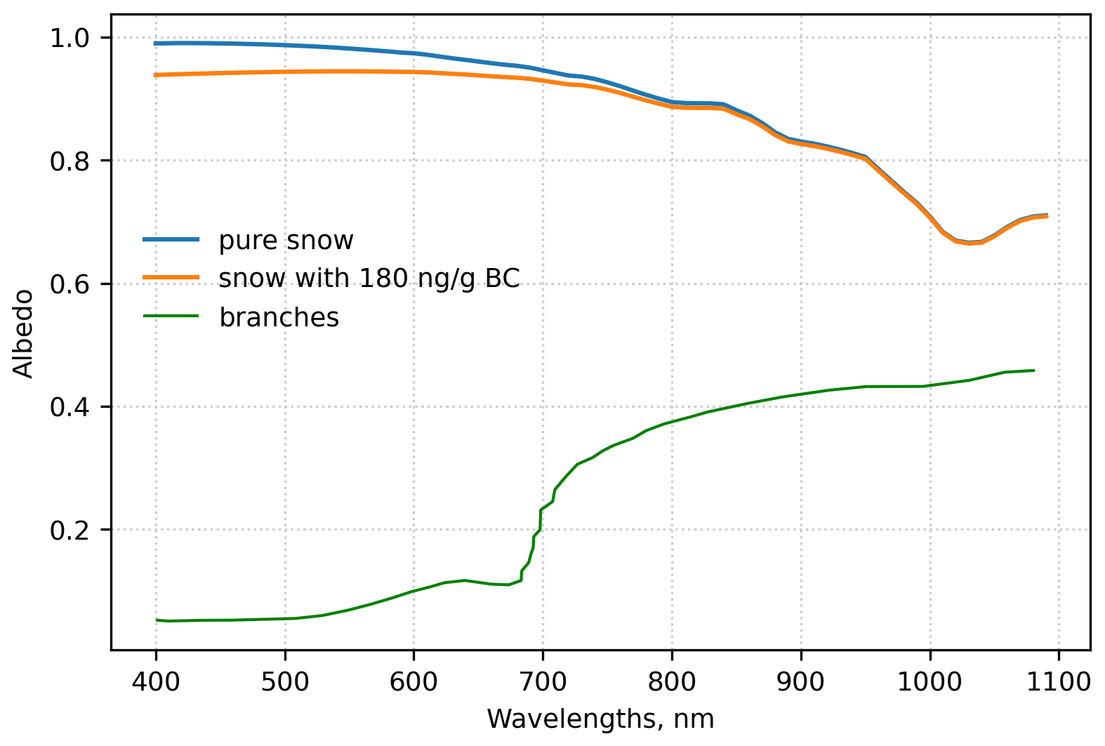
Figure 1 Comparison of the spectral albedo of pure snow (blue), dirty snow with 180 ng g⁻¹ of BC (orange) and branches (green). Albedo of branches was determined from measurements taken by Juszak et al. (2014). Branch absorption is strongly wavelength dependent and decreases sharply for wavelengths >680 nm.

Irradiance in snow and the effect of LAPs are generally computed numerically with radiative transfer models (Warren and Wiscombe, 1980; Hansen and Nazarenko, 2004; Aoki et al., 2011; Tuzet et al., 2017). Today, it is possible to calculate radiative transfer through snow as a function of snow physical properties (i.e. snow density, specific surface area (SSA) and grain shape), using the analytical equations established by Kokhanovsky and Zege (2004). For LAPs, the radiative effect is calculated for pre-established impurity concentrations using the optical properties that are associated with the different impurity types (i.e. the impurity-specific mass absorption efficiency, MAE). However, from a radiative transfer modelling point of view, branches and LAPs are very different objects, and their radiative effect in the snowpack cannot be calculated in the same way. LAPs are homogeneously mixed with snow so that their absorption can be averaged and combined with that of the ice, and the classical solution of the radiative transfer equation for homogeneous media applies without any change. These LAPs are externally mixed with snow; i.e. they are not incorporated inside the snow grains. In contrast, branches are macroscopic embedded absorbers that affect the path of light, a situation that has no simple analytical solution. To design a model that accurately represents buried branches and allows calculation of their specific radiative impact, it is first necessary to acquire basic knowledge about how snow, light and buried branches interact.

This study aims to bring the first insights, to our knowledge, on how buried branches influence light propagation in snowpacks. We present a qualitative analysis where we use a combination of in situ measurements and radiative transfer simulations. The latter were computed with the radiative transfer model SnowMCML (Picard et al., 2016) for snowpacks with known snow physical properties and estimated impurity type and concentrations. In situ data were acquired during a field campaign in Umiujaq, Northern Quebec (56.5^∘ N, 76.5^∘ W), in autumn 2015 and consisted of (i) vertical spectral irradiance profiles (350–900 nm) measured in snowpacks with and without shrubs and (ii) vertical profiles of snow density and SSA measured in snowpits. Impurity concentrations and types were estimated from optical measurements taken in shrub-free snowpacks. The effect of buried branches was investigated by comparing irradiance profiles measured in shrub snowpacks with SnowMCML simulations that include LAPs estimated from irradiance profiles measured in shrub-free snowpacks.

2 Study site and data acquisition

2.1 Study site

Our study site is located near the village of Umiujaq on the coast of Hudson Bay in Nunavik, Northern Quebec (56^∘33^′07^′′ N, 76^∘ 32^′57^′′ E, Fig. 2). Measurements were taken in Tasiapik Valley, ∼ 4 km from Umiujaq village. The study sites happen to also be ∼ 2 km from a waste disposal site, where waste was occasionally burned in open-air conditions. All measuring sites were situated on a wind-exposed plateau, with sites situated in the northern part of the plateau (Fig. 2 and Table 1) being slightly windier and with slightly less snow. The distance between the sites on the northern and southern parts of the plateau was around 1 km. The plateau is covered with lichen and shrubs, but stands of black spruces (Picea mariana) which are relicts of past warmer periods (Payette and Morneau, 1993) are also found in the southern area of the plateau (Gagnon et al., 2019). Over the last 3 decades, Nunavik has experienced the strongest greening trend in North America (Ju and Masek, 2016). This is due to shrubs expanding in the tundra biome and replacing lichen patches of mostly Cladonia spp. (Ropars and Boudreau, 2012; Provencher-Nolet et al., 2014; Gagnon et al., 2019). In the Umiujaq region, the main shrub species are birches (Betula glandulosa), willows (mostly Salix glauca and S. planifolia) and alders (Alnus viridis subsp. crispa). An automatic weather station has been recording climatic data in the Tasiapik Valley since 1997 (Fig. 2). From 1997 to 2018, the mean annual air temperature has been −3^∘ C (CEN, 2018). In the region of Umiujaq, strong winds and snowstorms are frequent, and wind speeds can reach up to 100 km h⁻¹ (Barrere et al., 2018). The predominant wind direction is from the bay (west and northwest) (Paradis et al., 2016), and our measuring sites are thus mostly downwind from the village and the waste burning site as shown by the wind rose in Fig. 2. The wind rose was calculated using wind data from September to December that were collected by the automatic weather station (AWS) from 2012 to 2019. After analysis of the snow optical data, it seemed very likely that fumes from the waste burning in open air could have reached our measuring sites and probably affected the acquired data when wind speeds were high enough.

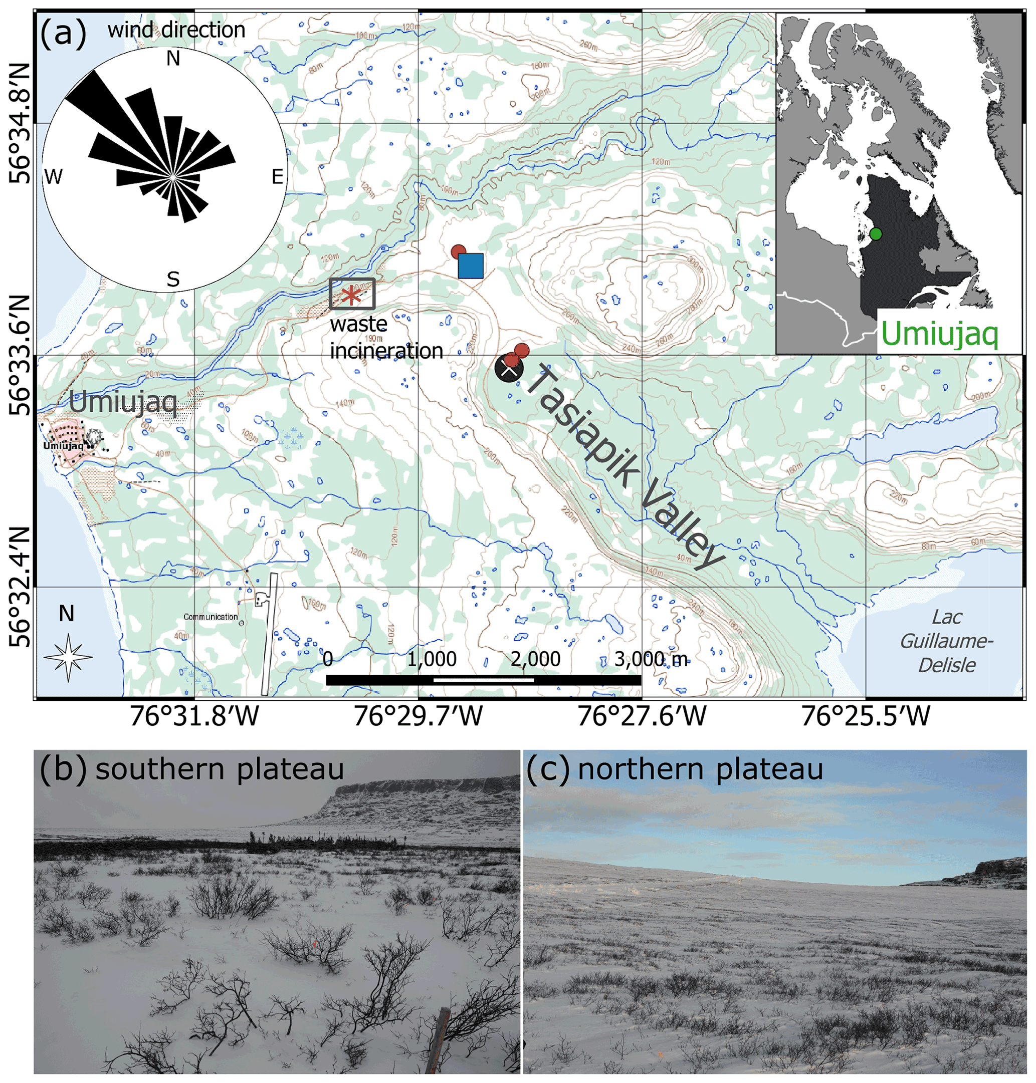
Figure 2 Map and photos of the study area in the Tasiapik Valley near the village Umiujaq. (a) In the map, the blue rectangle marks the area where irradiance profiles were measured in shrub-free snowpacks, the red dots mark where irradiance profiles were measured in snowpacks with shrubs, and a white cross marks the position of the automatic weather station (AWS). The site where waste was burned is denoted with a red star. The general wind direction for the time period from September to December is given by a wind rose and was calculated using data collected by the AWS from 2012–2019. (b) Landscape around sites in the southern plateau area and (c) landscape around measuring sites in the northern plateau area. Map source: Natural Resources Canada (http://atlas.gc.ca/toporama/en/index.html, last access: September 2016).

Table 1 Snow height and shrub height in Umiujaq for the three shrub-free snowpacks and the four snowpacks with shrubs.

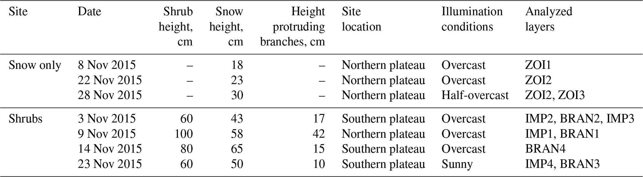
Data were acquired during a field campaign from 29 October to 6 December 2015. During that period, snow and irradiance measurements were taken at four sites with shrubs and three sites with a shrub-free snowpack. Snow and irradiance measurements are destructive and could therefore only be taken once for each site. Measurements in snowpacks with shrubs were conducted on 3, 9, 14 and 23 November. Snow height at these sites varied between 43 and 63 cm, shrub height varied between 60 and 100 cm, and the height of protruding branches varied between 10 and 42 cm (Table 1). The differences in shrub height (Table 1) indicate the intra-site variability. Measurements in shrub-free snowpacks were conducted on 8, 22 and 28 November, and snow height at these sites varied between 18 and 30 cm (Table 1). All shrub-free sites were within a range of ∼ 10 m from each other and are considered comparable with similar topography and wind exposure. We aimed to conduct measurements for shrub and shrub-free snowpacks at weekly intervals, but harsh measuring conditions and frequent blizzards often prevented us from maintaining this regular measuring interval.

2.2 Data acquisition

2.2.1 Spectral irradiance profiles

Vertical irradiance in the snowpack was measured with the SOLar EXtinction in Snow profiler (SOLEXS). The instrument was developed and tested by Libois et al. (2014) and Picard et al. (2016), where a full description and schematic illustrations can be found. Basically, the SOLEXS instrument consists of an optical fibre cable which is inserted into a metallic rod painted in white (colour: RAL 9003). The rod (10 mm diameter) is vertically inserted in the snowpack into a hole of the same diameter which was punched by a metal rod prior to the measurement. Throughout the continuous manual descent and subsequent rise of the rod in the hole, its position is registered with a depth sensor with a resolution of 1 mm. The optical cable is connected to an Ocean Optics MayaPro spectrometer with a spectral range of 300 to 1100 nm and a resolution of 3 nm. Here, we use measurements from 350 to 900 nm only because the signal-to-noise ratio is too low outside this range. Spectral radiation is recorded every 5 mm while the rod is continuously moving down and up the hole. The maximum acquisition depth is ∼ 40 cm. Below 40 cm the signal-to-noise ratio becomes too low because of the reduced light intensity, and the shadow of the operator cannot be neglected past this point (Libois et al., 2014), as detailed in Picard et al. (2016). The acquisition of one irradiance profile took around 2 min once the instrument was deployed. A photosensor was placed at the snow surface to monitor the incident radiation changes during the acquisition. If changes in incident radiation exceeded 3 %, the measurement was discarded. Measurements were conducted during any lighting conditions, i.e. overcast, partially overcast and sunny.

SOLEXS is accompanied by a post-processing library (Picard et al., 2016). This library automatically deploys the following processing to the recorded profiles: (1) subtraction of the dark current, (2) a depth correction using the small difference of timestamps between the depth and spectrum acquisitions, and (3) normalization by the photosensor current to correct for the small fluctuation of irradiance during the complete acquisition.

2.2.2 Snowpit data

After each acquisition of a SOLEXS profile, we dug a snowpit at the same spot. In the snowpit, the snow stratigraphy was recorded and photographed, vertical profiles of snow density and snow specific surface area (SSA) were measured, and, in snowpacks with shrubs, the presence of branches was noted. Snow density profiles have a resolution of 3 cm and were measured with a 100 cm³ box cutter (Domine et al., 2016). SSA is the surface area of the snow–air interface per mass unit and is inversely related to the optical grain diameter of snow (Warren, 1982; Domine et al., 2007). SSA was acquired with the DUFISSS instrument detailed in Gallet et al. (2009). Briefly, DUFISSS measures the infrared reflectance of snow samples at 1310 nm by using an integrating sphere. SSA is then calculated from that reflectance with a simple algorithm (Gallet et al., 2009). SSA profiles were measured with a resolution of 1 to 3 cm.

Knowing snow density and SSA allows calculation of the light absorption efficiency of pure snow by using radiative transfer theory (Kokhanovsky and Zege, 2004; Picard et al., 2016). For these calculations, density and SSA need to be available with the same depth resolution. Where this was not the case in our data set, we performed linear interpolation between measured density data points, in order to synchronize the SSA and density profiles.

3 Methodology

3.1 Overview of methods

SOLEXS records the irradiance intensity at different depths (I(z)) and thus shows how much light is transmitted through the snowpack. The intensity of transmitted light decreases with depth either because radiation gets absorbed or because it is scattered, which provokes a change in the light path direction. The processes of scattering and absorption together are called extinction. In a pure snowpack, extinction is mainly due to scattering. In contrast, impurities in the snowpack as well as buried branches cause light to become extinct mainly through absorption. Hence, when referring to light–impurity or light–branch interactions, for all practical purposes extinction and absorption can be used synonymously. In this study we are interested in comparing the extinction of light with depth in snowpacks with and without shrubs. This extinction is visualized as log-irradiance profiles (I_log(z,λ)):

$$\begin{array}{}\text{(1)}& I_{\log }\left(z,\mathit{\lambda }\right)=\log \left(I_{\mathrm{0}}\left(\mathit{\lambda }\right)/I\left(z,\mathit{\lambda }\right)\right),\end{array}$$

where I₀ is the incoming radiation at the surface, z is snow depth, λ is wavelength and (I(z,λ)) represent the measured SOLEXS profiles. Hence, to obtain I_log(z,λ) from the measured data, SOLEXS profiles were normalized with I₀(λ) and then presented in log scale. Here, the surface irradiance values for normalization are obtained at a depth of 3 cm ($z=-\mathrm{3}$), because the presence of direct light may influence measurements at shallower depths.

Snowpacks are heterogeneous media made up of several kinds of light-extinctive materials – i.e. snow, light-absorbing particles (LAPs) and, for snowpacks with shrubs, buried branches. During SOLEXS acquisitions, the measuring rod inserted into the snowpack also contributes to light extinction (Picard et al., 2016). If the interaction between the different light-extinctive materials is negligible, the log-irradiance profile in the medium I_log(z,λ) is the sum of the material-specific terms. In snowpacks with shrubs this is calculated as

$$\begin{array}{}\text{(2)}& \begin{array}{rl}{I}_{\log }\left(z,\mathit{\lambda }\right)& =E_{\mathrm{snow}}\left(z,\mathit{\lambda }\right)+E_{\mathrm{rod}}\left(z,\mathit{\lambda }\right)+E_{\mathrm{LAP}}\left(z,\mathit{\lambda }\right)\\ & +E_{\mathrm{shrub}}\left(z,\mathit{\lambda }\right),\end{array}\end{array}$$

where E_snow, E_LAP,E_shrub and E_rod represent the material-specific extinction of snow, impurities, shrubs and the measuring rod, respectively. In order to evaluate the extinction due to buried branches E_shrub from measured I_log profiles, E_snow, E_rod and E_LAP need to be calculated or estimated.

The approach presented here is a simplification, and more physically based approaches can be imagined where the influence of branches would be calculated with sophisticated 3D radiative transfer models. Such an approach would require complex simulations and to precise characterizations of the optical and physical properties of our medium (i.e. the snowpack with branches and impurities). However, at this stage, very little is known about the influence of branches on radiative transfer in snow. We therefore gave precedence to this simpler and more straightforward approach to obtain first insights into the buried branch–snow–light interactions.

To determine the amount of light absorption by branches, we applied three successive steps. (i) First, light extinction by pure snow and the measuring rod (E_snow+E_rod) was calculated with a radiative transfer model as a function of in situ measured snow physical properties (Sect. 3.2). (ii) Next, the light absorption of impurities (E_LAP) was estimated using two complementary methods that allow retrieval of impurity information from the irradiance profiles measured in shrub-free snowpacks (Sect. 3.3). (iii) Finally, based on the information acquired on E_snow, E_rod, and E_LAP in the two previous steps, we determined the influence of buried branches in the irradiance profiles measured in snowpacks with shrubs using Eq. (2).

3.2 Calculation of light extinction by snow and the measuring rod

The 3D radiative transfer model SnowMCML was used to compute the combined light extinction of snow and the measuring rod (E_snow+E_rod). SnowMCML was developed by Picard et al. (2016) and is based on the model “Monte Carlo modeling of light transport in multi-layered tissues” (MCML) from Wang et al. (1995). Specifically, Picard et al. (2016) adapted the model to compute the signal recorded at the tip of a rod inserted in a multi-layered snowpack. The snow physical properties of each snow layer are supposed to be known, as well as the absorption of the rod. A detailed description of the model is given in Picard et al. (2016). Briefly, the model traces N light rays through a multi-layered snowpack with known physical properties. At each calculation step, light absorption and scattering are determined, and the associated decrease in intensity for each light ray is calculated. To optimize calculation time, the model uses the inverse principle in optics, launching rays from the collector tip and tracing them back to the source at the surface instead of launching rays at the surface. Using this inverse mode allows the calculation of only the path of those rays that hit the collector and which are thus relevant to compute the signal recorded at the tip of the rod. The size and optical properties of the rod need to be known to implement its effect in the simulations. Following the indications from Picard et al. (2016), the rod was modelled as a cylinder with a 10 mm diameter and a length corresponding to the insertion depth of the rod. The albedo of the rod (ω_rod) was set to 0.9 based on the reflectance measurements of the paint conducted by Picard et al. (2016), and it was assumed that the rod had Lambertian scattering characteristics; i.e. rays hitting the rod are scattered in a random direction. In the simulations, the rays hitting the rod were absorbed with a probability 1−ω_rod.

In addition to the size and optical properties of the rod, input data to SnowMCML were the physical properties of snow measured in the snowpits. The model outputs were theoretical transmittance profiles. These profiles show light transmittance for a snowpack without LAPs and branches, but with the same physical properties (SSA and density) as the snowpacks investigated. The simulated I(z,λ) profiles were normalized and converted to log scale to obtain the log-irradiance profiles (I_log(z,λ)) from Eq. (1). These profiles were then compared with the log-irradiance profiles acquired in the field.

At transition zones, the performance of the model was found to be limited. These zones include the snow–atmosphere transition in the uppermost layer, the transition between two stratigraphic layers inside the snowpack or the transition from snow to the underlying soil layer at the bottom of the snowpack. Discrepancies at the snow–atmosphere transition are probably caused by the rod entering the snowpack and causing an optical disturbance. Moreover, close to the surface and down to −7 cm, direct light can potentially penetrate the snowpack and come in through holes around the measuring rod as detailed by Picard et al. (2016). Since the presence of direct light is known to perturb the measured irradiance profiles (Picard et al., 2016; Tuzet et al., 2019), we discarded the first 7 cm in measured and simulated log-irradiance profiles. At stratigraphic transitions inside the snowpack, a mismatch between the model and the measured log-irradiance can be due to uncertainties in the snow physical properties that are used as input to the model. These arise because snow physical properties often change gradually or are heterogeneous in stratigraphic transition zones. These fine-scale changes are not captured by our measuring profiles with a resolution of 1 to 3 cm, leading in turn to inaccuracies in the simulations compared to processes in the natural snowpack. Moreover, rod–light interactions that are calculated in the model also depend on snow physical properties, which can further amplify the discrepancies between the simulated and measured irradiance profiles.

An additional particularity at stratigraphic transition zones is the occasional occurrence of positive irradiance gradients (Picard et al., 2016). These are caused by different interactions between the rod and radiation in each snow layer near the layer transition. These interactions are complex and are explained in detail by Picard et al. (2016). Intuitively, when the rod reaches a lower layer, the magnitude of the artefact it causes is determined by interactions between the rod and the layer above, and in some cases, this can result in an increase in the measured signal, even though the radiative transfer in a 1D layered media excludes positive irradiance gradients. Although SnowMCML accounts for the rod artefact at transition zones and can calculate associated positive gradients, their occurrence in simulated and measured profiles may not concur if there are uncertainties in the snow physical properties that are used as input to the model. For this reason, we excluded transition zones, i.e. the top and bottom of each layer, from the interpretation of SnowMCML simulations.

3.3 Estimation of absorption by LAPs

Determining the specific absorption of LAPs (E_LAP) with radiative transfer models requires that concentrations of LAP be given and that the optical properties for a given impurity type be known. Unfortunately, there are no data on LAPs for the snowpack near Umiujaq. Therefore, we assumed that LAPs are either mineral dust coming from a local source (hereafter called dust) or black carbon (BC). Dust can be transported from the cliffs and the barren rock surfaces at the top of cuestas to the valley during windy autumn storms which are typical for this region (Barrere et al., 2018; Paradis et al., 2016). BC is typically introduced to Arctic snow through long-range transport from fossil fuel combustion in the south (McConnell et al., 2007; Doherty et al., 2010). Based on field observations it seems likely that BC was also produced by snowmobile traffic in the valley and, perhaps more importantly, by the waste burning occurring ∼2 km upwind from our study site (Fig. 2). Based on these assumptions, we employed two methods to estimate the relative concentration of BC and mineral dust.

The first method applies a regression approach to in situ data while the second uses SnowMCML to simulate radiative transfer in a snowpack with impurities. Both methods are similar in that they determine impurity type and concentration. The advantage of the SnowMCML method is that the model considers the influence of the measuring rod, but the disadvantage is that it assumes homogeneous impurity concentrations for the entire snowpack. In contrast, the regression method neglects the impact of the measuring rod but allows determination of LAP concentrations for different layers individually. We applied the two complementary methods to validate results from each other. Finally, both methods were verified against log-irradiance measured in shrub-free snowpacks, where LAPs were the only unknown light-absorbing material. The two methods are detailed in the following sections.

3.3.1 Regression analysis of experimental profiles

In the first approach, information on LAP concentrations is derived from the irradiance profiles I(z,λ) measured with SOLEXS by analyzing the rate of decrease in light intensity with snow depth following Tuzet et al. (2019). In snow layers with optically homogeneous conditions, light intensity decreases exponentially (Beer–Lambert law). Using logarithmic plots allows this exponential decrease to appear linear, and the rate of decrease for a specific snow layer is then obtained from the slope of a linear regression (Fig. 3a). In the literature, this rate of decrease is commonly referred to as the asymptotic flux extinction coefficient (e.g. Libois et al., 2013), but for the sake of simplicity we will refer to it as the extinction coefficient, k_e. The rate by which light decreases in the snowpack is wavelength-dependent, and k_e is thus usually shown as a spectral curve termed k_e(λ) (Fig. 3b). k_e also depends on the physical properties of the snowpack (SSA and density ρ) and on the type and concentrations of LAPs mixed in the snowpack. For example, the k_e(λ) curve for a dirty snowpack would display higher k_e values than a clean snowpack because the former is a much more absorbing medium and thus absorbs light at a greater rate. Consequently, each snowpack layer has a specific spectral curve k_e(λ) which is a function of the physical properties of the layer as well as the type and concentration of the LAPs mixed in the snowpack. This relation is mathematically expressed as (Libois et al., 2013; Tuzet et al., 2019):

$$\begin{array}{}\text{(3)}& k_{\mathrm{e}}\left(\mathit{\lambda }\right)=\sqrt{{\displaystyle \frac{\mathrm{3}\left(\mathrm{1}-g\right)}{\mathrm{2}}}{\mathit{\rho }}^{\mathrm{2}}\mathrm{SSA}\left({\displaystyle \frac{B{\mathit{\gamma }}_{\mathrm{ice}}\left(\mathit{\lambda }\right)}{{\mathit{\rho }}_{\mathrm{ice}}}}+\mathrm{MAE}\left(\mathit{\lambda }\right)c\right)},\end{array}$$

where γ_ice is the ice absorption index which was set to the most recent estimate from Picard et al. (2016). B is the ice absorption enhancement factor and g the scattering asymmetry factor, which were set to default values of 1.6 and 0.85, respectively (Libois et al., 2014). ρ_ice is the density of ice (917 kg m⁻³), and finally, c is the LAP concentration in kg kg⁻¹ and MAE is the mass absorption efficiency (m² kg⁻¹) describing the optical property of a given LAP type (Caponi et al., 2017). For this study, the impurity type and the associated MAE values were set to either dust or BC. To determine LAP concentrations in the Umiujaq snowpack, the k_e(λ) curve deduced from SOLEXS measurements (Fig. 3) (k_{e_meas}(λ)) was fitted to the k_e(λ) curve calculated with Eq. (3) (k_{e_calc}(λ)). To fit both curves, the LAP concentration (c in Eq. 3) was estimated using Python's scipy.optimize.least_squares function which minimizes the mean square error between k_{e_calc}(λ) and k_{e_meas}(λ). The final best fit between the k_{e_calc}(λ) and k_{e_meas}(λ) curves in the spectral range considered (350–900 nm) was evaluated with the coefficient of determination (R²), and the error was given by the root mean square error (RMSE). R² was calculated with

$$\begin{array}{}\text{(4)}& R^{\mathrm{2}}=\mathrm{1}-({\mathrm{SS}}_{\mathrm{total}}/{\mathrm{SS}}_{\mathrm{res}}),\end{array}$$

where SS_total is the sum of squares of the vertical distance of all points to a horizontal line (called the null hypothesis), and SS_res is the sum of squares of the vertical distance of all points to the model (Motulsky and Christopoulos, 2003).

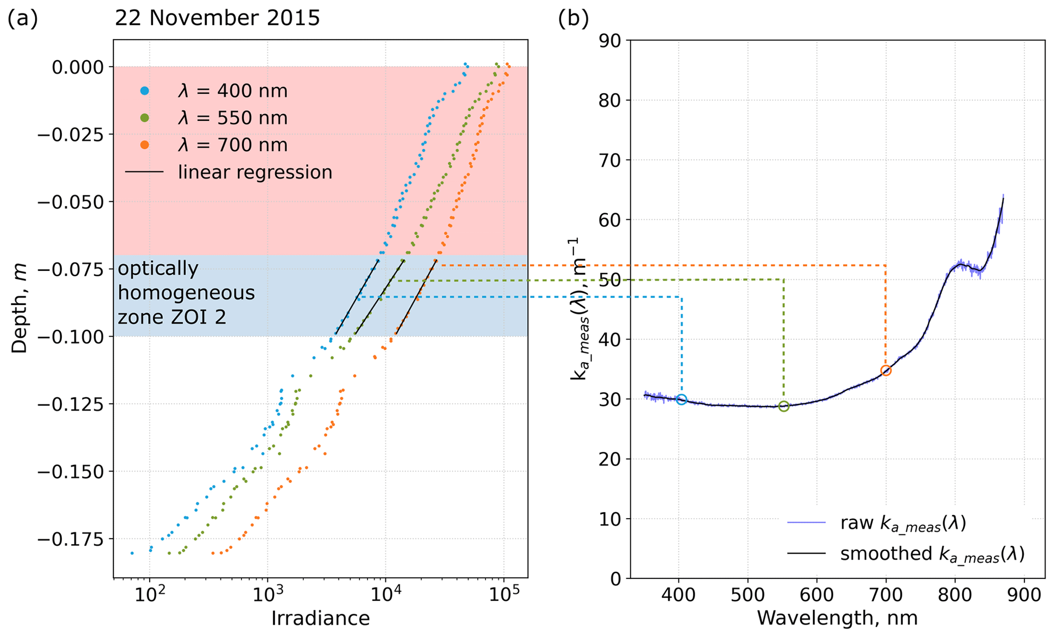
Figure 3 Overview of how the extinction coefficient (k_{e_meas}(λ)) was determined from optically homogeneous layers in irradiance profiles. (a) Irradiance as a function of depth for selected wavelengths. The blue shaded area highlights an optically homogeneous zone where the recorded signal is linear on a logarithmic scale. The red shaded area was discarded due to potential influence of direct light. k_{e_meas}(λ) is the slope of the linear regression of irradiance vs. depth in the optically homogeneous zone (black lines). (b) k_{e_meas}(λ) determined for each wavelength in the measured spectrum (350–900 nm) before (blue curve) and after smoothing (black curve). The figure layout was adopted from Tuzet et al. (2019) and modified using data measured near Umiujaq on 22 November 2015. The blue shaded area is subsequently referred to as ZOI2.

Following Tuzet et al. (2019), k_{e_meas}(λ) curves were only determined for layers where the optical properties in the snowpack were homogeneous for at least 3 consecutive centimetres, and the recorded SOLEXS signal was visually linear, because deducing a slope via linear regression is only possible under these conditions. These layers where k_{e_meas}(λ) could be calculated are hereafter called zones of interest (ZOIs). According to Tuzet et al. (2019), ZOIs have to be at least 3 cm thick and lie at a snow depth >7 cm because at shallow depths and around transition zones the k_{e_meas}(λ) determination can be biased by the impact of the SOLEXS measuring rod (discussed in Sect. 3.1; Picard et al., 2016). k_{e_meas}(λ) curves were smoothed using a first-order Butterworth filter with the scipy.signal.butter function in Python (cutoff frequency set to 0.05; Fig. 3b). The spectrum used to fit k_{e_meas}(λ) and k_{e_calc}(λ) ranged from 400 to 450 nm. In this range absorption by ice is lowest, and impurities thus have the strongest impact on absorption profiles. Constraining the fit to a specific range instead of using the entire spectrum (350–900 nm) allows us to test the hypothesis that BC or dust is the principal impurity type. A good fit between 400–450 nm should also return a good fit at wavelengths >450 nm if the spectral absorption of the absorbers was chosen correctly.

3.3.2 SnowMCML simulation

SnowMCML allows the simulation of the effect of light-absorbing impurities for snowpacks with given LAP concentrations and MAE values for a given LAP type. For dust, the MAE was taken from Caponi et al. (2017) choosing an Algerian dust type, with a grain diameter of 10 µm. Algerian dust was chosen because its optical properties (in particular its Ångström absorption exponent) are similar to those of the typical dust reported for snow in the Canadian sub-Arctic (2.5 for Algerian dust vs. 2.2 for sub-Arctic impurities) (Doherty et al., 2010). The relatively large grain diameter of 10 µm (vs. 2 µm) was chosen because we assumed the dust source to be local. For BC, we followed the approach of Tuzet et al. (2019) and determined the MAE from the studies of Bond and Bergstrom (2006) and Hadley and Kirchstetter (2012). SnowMCML simulations were then computed with a variety of BC and dust concentrations. Note that each simulation corresponds to one LAP concentration as SnowMCML simulated radiative transfer assuming homogeneous LAP concentrations in the entire snowpack. BC or dust concentrations were determined by fitting the simulations with known LAP concentrations to the measured log-irradiance profiles with unknown concentrations. The snow–atmosphere transition zone (0 to −7 cm) and the stratigraphic transition zones were excluded from the fit as explained above. From the remaining non-transition layers, LAP type and concentrations were deduced from simulations that most accurately represented the radiative effect in the snowpack in Umiujaq. These best-fitting simulations were determined from a visual comparison of the simulated and measured profiles in shrub-free snowpacks.

4 Results and discussion

4.1 Impurity type and concentration in snow without shrubs

The objective of the impurity analysis was to obtain representative impurity concentration values and to test the validity of our initial assumption that the significant LAPs were either mineral dust or BC. For this, LAP type and concentrations were determined from log-irradiance profiles measured in shrub-free snowpacks on 8, 22 and 28 November by using the two methods, i.e. the k_e analysis (Fig. 4) and the SnowMCML method (Fig. 5). Both methods are complementary but should ideally yield similar results for the deduced LAP type and concentration. For the LAP analysis we identified four zones (ZOI1 to ZOI4) where optical and physical snow properties were homogeneous (Fig. 5). Two of the four zones were in snowpits measured on 8 and 22 November (ZOI1 and ZOI2), and the other two were in the snowpit of 28 November (ZOI3 and ZOI4; Fig. 5 and Table 2). Within these zones we compared the fit between k_{e_meas}(λ) and k_{e_calc}(λ) as well as the fit between measured irradiance profiles and SnowMCML simulations.

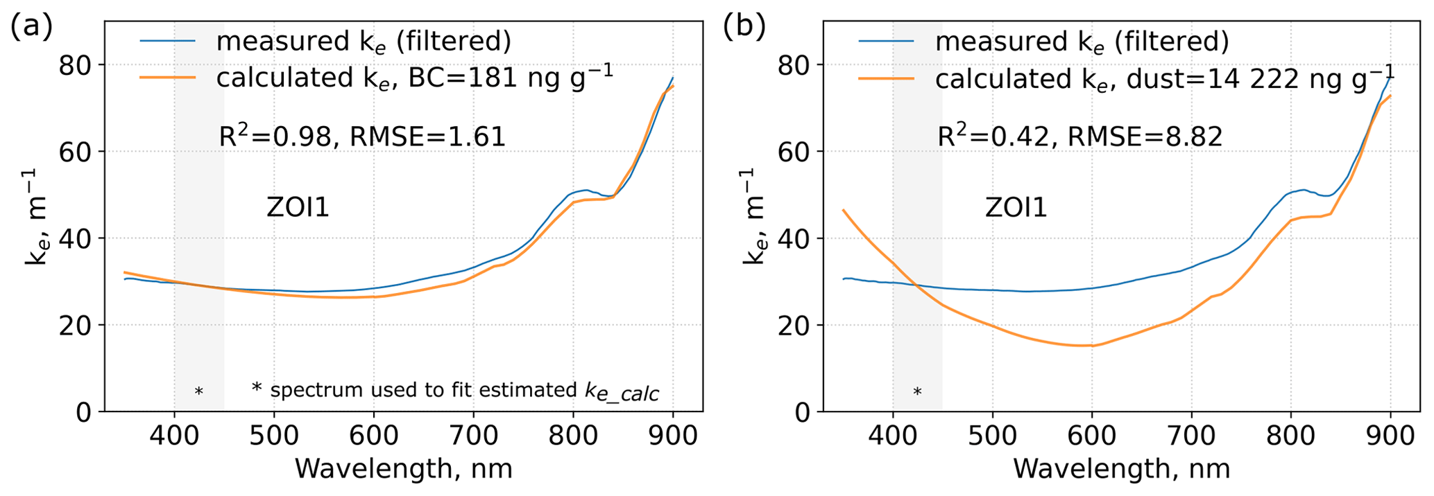
Figure 4 Example for measured and calculated absorption coefficient k_e for a snowpack without shrubs. Measured k_e was determined from SOLEXS measurements taken on 8 November (ZOI1). Calculated k_e was computed with either (a) black carbon (BC) or (b) mineral dust as impurity type in the snowpack. The concentration of dust or BC was determined with an iterative approach, where calculated k_e was fitted to the measured k_e. This example shows how assuming BC as impurity type returns significantly better fits.

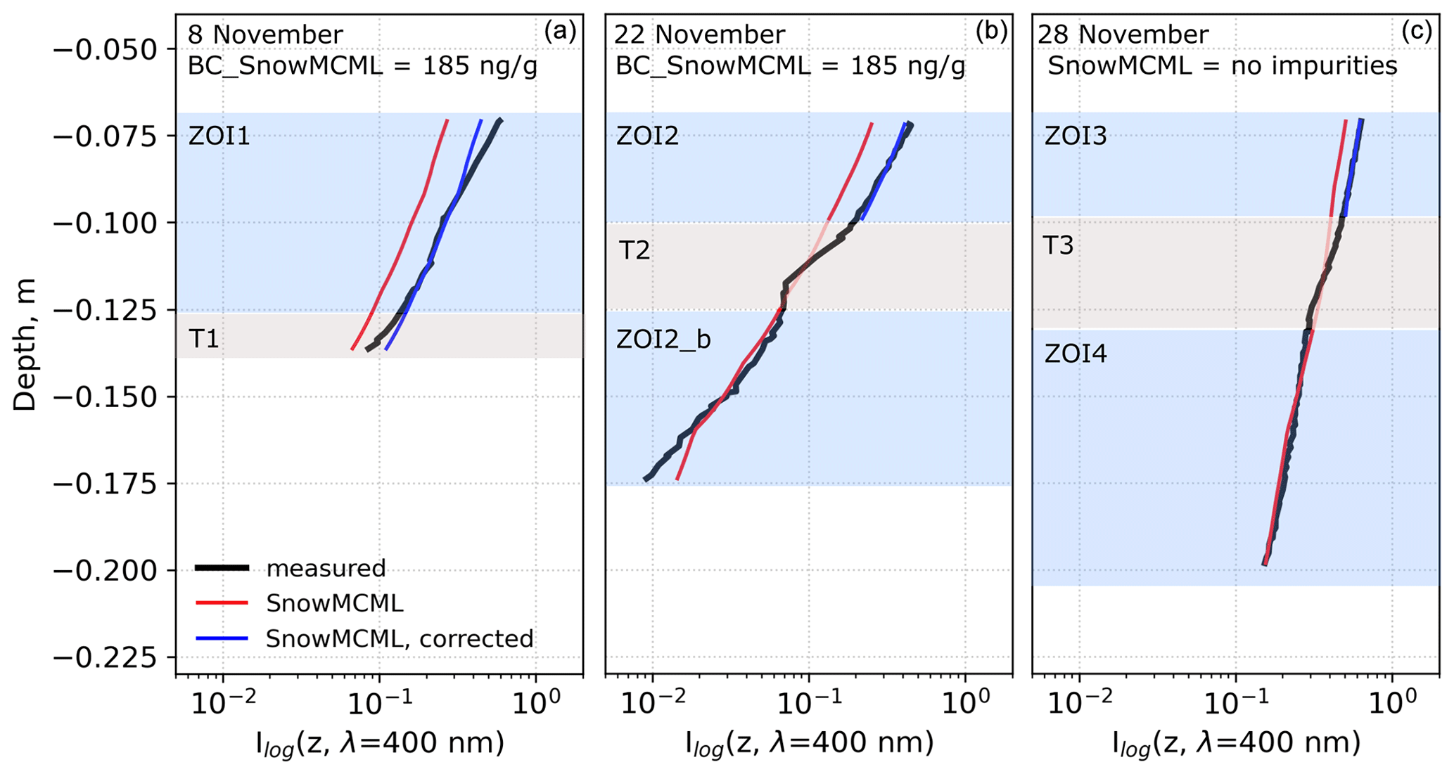
Figure 5 Measured log-irradiance profiles (black curves) and SnowMCML simulations (red and blue curves) for snowpacks without shrubs at 400 nm. Simulated profiles were computed assuming black carbon (BC) as the impurity type. Log-irradiance profiles were measured on (a) 8 November, (b) 22 November and (c) 28 November. Grey shaded areas highlight transition zones, where simulated and measured profiles were not expected to fit. Blue shaded areas highlight non-transition zones where the fit between simulated and measured profiles allowed the determination of impurity concentrations. A constant correction factor was applied to the simulated data in those layers where the extinction gradients were similar to the measured values but the profiles were parallel instead of overlapping. Correction factors were 0.61 (a, b) and 0.8 (c).

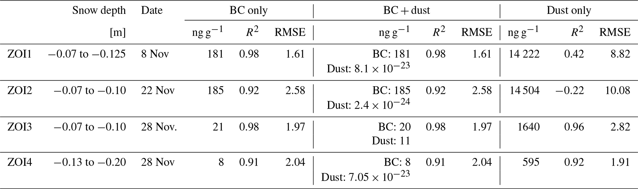
Table 2 Fit between measured and calculated extinction coefficient curves (k_e(λ)) for measurements in shrub-free snowpacks. Calculated k_e(λ) was computed with black carbon (BC), BC and mineral dust, or mineral dust only. The fit between measured and calculated k_e(λ) was analyzed with the coefficient of determination (R²); the error is indicated with the root-mean-square error (RMSE).

4.1.1 Results from the k_e analysis

The results of the fit between k_{e_meas}(λ) and k_{e_calc}(λ) shown in Table 2 highlight that impurity concentrations were variable between the different snowpits. For snowpits measured on 8 and 22 November (ZOI1 and ZOI2), the k_e analysis returned high impurity concentrations, whereas the snowpit measured on 28 November (ZOI3 and ZOI4) had comparatively lower values. For the high-impurity zones ZOI1 and ZOI2, setting the LAP type to BC in Eq. (3) constantly returned a very good fit between the estimated and measured k_e curves. For example, in ZOI1 the achieved fit had a R² value of 0.98 and a RMSE of 1.61 (Fig. 4a) when LAP was set to BC. The fit was good for all wavelengths in the spectrum considered (350–900 nm), suggesting that the spectral absorption signature of BC is well suited to reproduce the extinction coefficients observed in ZOI1 and ZOI2. In contrast, setting the LAP type to dust in Eq. (3) (Fig. 4b) resulted in visibly poor fits between k_{e_meas}(λ) and k_{e_calc}(λ) curves (R²=0.42; RMSE = 8.82). The fit was poor for the entire spectrum, but the direction and magnitude of the mismatch was wavelength-dependent, suggesting that the spectral absorption signature of dust was ill-suited to reproduce the extinction coefficients observed in ZOI1 and ZOI2. For the low-impurity zones (ZOI3 and ZOI4), using BC only, dust only, or dust and BC in Eq. (3) returned consistently low impurity concentrations with similarly good fits for all impurity types. For example, in ZOI3 the best fit (R²=0.98) was achieved by using BC only, while using dust only reduced the fit slightly (R²=0.96). For ZOI4 the best fit (R²=0.92) was achieved by using dust only, while using BC only reduced the fit slightly (R²=0.91). Results for all four ZOIs are listed in Table 2.

4.1.2 Results from SnowMCML simulations

For the SnowMCML method, the same ZOI layers were used as for the k_e analysis (ZOI1–ZOI4, highlighted in blue in Fig. 5), plus one additional layer (ZOI2_b, Fig. 5). Transition zones (T1–T3 in Fig. 5) were excluded from our analysis because they had no homogeneous snow optical and physical properties. The additional layer ZOI2_b was only used for the SnowMCML analysis because its signal-to-noise ratio at longer wavelengths was too weak to establish a spectral k_{e_meas}(λ) curve. The results of the SnowMCML simulations concur with the results of the k_e analysis. For the high-impurity zones ZOI1 and ZOI2 measured on 8 and 22 November, using BC concentrations of 185 ng g⁻¹ returned a good and wavelength-independent agreement between the simulated profiles and the measured log-irradiance profiles (Fig. 5a and b). Note that in these layers the simulations with BC showed the same extinction gradient as the measured data but with an offset. Consequently, simulated and measured profiles were parallel to each other in ZOI1 and ZOI2 instead of being superposed. The reason for the offset was probably that the amount of light transmitted to ZOI1 and ZOI2 from the transition zone was inaccurately calculated by the model. The fit between simulations with mineral dust and the measured data in ZOI1 and ZOI2 was not as good as shown in the Supplement (S2). For the low-impurity zones ZOI3 and ZOI4 the best fit for the SnowMCML profile was obtained for the simulation without impurities, which agrees with the overall low impurity concentrations determined with the k_e analysis.

4.1.3 BC as a significant absorber

We conclude from the k_e analysis and SnowMCML simulations that BC is the significant absorber in snow without shrubs. However, for the snowpack measured on 28 November, using dust instead of BC in simulations also returned a good fit, and it is likely that some trace amounts of dust, coming from the cuestas surrounding Tasiapik Valley, were also present in the snow. Nevertheless, the overall impurity concentrations on 28 November were very low (Table 2) and the good fit for the SnowMCML profile simulated without impurities suggests that impurity impact on absorption was negligible in those cases (Fig. 5c). This is, of course, a simplification, and a chemical analysis of LAPs in snow would nicely complement these optical studies, but this is left for future work. Based on our current data, we conclude that light extinction in snow without shrubs is best modelled with BC as the main impurity type. This is also consistent with other studies in the Arctic that have found BC to be the main impurity type in Arctic snow (e.g. Doherty et al., 2010; Wang et al., 2013). Moreover, the open-air waste burning near our study area was probably an important additional BC source (Fig. 2). For the purpose of this study we will therefore assume that BC is the dominant impurity type in the Umiujaq snowpack.

Unfortunately, BC concentrations were found to vary considerably among the shrub-free snowpacks, which prevented the determination of a representative BC concentration for the Umiujaq snowpack in general. Nevertheless, we obtained concordant results with both independent methods and we are thus confident in the BC concentrations reported here. The observation that BC concentrations have high spatiotemporal variability also fits with our previous interpretation that an important source of BC in Umiujaq snow was most likely the nearby irregular waste burning. Waste was not burned continuously, and the specific spatial deposition of BC would strongly depend on wind speed and direction during burning events. The snowpacks sampled on 8 and 22 November both had high BC concentrations, and the analyzed layers were probably accumulated during burning events. Accumulation could either have happened through direct precipitation or when a previously clean precipitated layer was drifted by wind through contaminated air masses and then redeposited in wind-sheltered areas. In contrast, the clean snowpack on 28 November was probably accumulated during a waste-burning-free period. It is important to note that despite the small increase in snow height from 22 and 28 November (only 7 cm), it is unlikely that the same snow measured on 22 November was still the surface snow layer on 28 November because of snow re-distribution by strong winds and melt events during warm spells. This explains how a snowpack with high BC could be measured on 22 November, while 1 week later on 28 November the snowpack was found to be clean with low BC concentrations. The spatiotemporal variability in BC concentrations is thus probably the result of discontinuous waste burning and the heterogeneous snow accumulation and erosion patterns due to wind drifting and precipitation.

4.2 Insights into the radiative effect of buried branches

Determining the effect of buried branches from the acquired log-irradiance profiles proved a complex task because we could not deduce a constant impurity concentration representative of the Umiujaq snowpack in general. Consequently, in Eq. (2), E_LAP(z) and E_shrub(z) both remain unknown variables in the log-irradiance profiles measured in snowpacks with shrubs. Furthermore, high BC concentrations had a strong impact on absorption, potentially masking the effect of branches. Nevertheless, interesting insights into how buried branches might influence light propagation were gained by (i) comparing SnowMCML simulations with the measured log-irradiance profiles and (ii) studying the spectral shape of k_{e_meas}(λ) and k_{e_calc}(λ) for different layers in snowpacks with branches.

4.2.1 Comparison of log-irradiance profiles with SnowMCML simulations

From the comparison of measured log-irradiance profiles with SnowMCML simulations at 400 nm, we found that snowpacks in shrubby areas consisted of two types of optically distinct layers (Fig. 6). Characteristics of the first layer type were that the measured profiles fitted well with the SnowMCML simulations (we called these layers IMP1 through IMP4 in Fig. 6), although the simulations only considered the extinction of light by snow, the measuring rod and BC, but not by shrubs. Moreover, photographs of the snowpits showed no or very few branches in these layers. The best examples for this layer type are IMP1 and IMP2, where the measured log-irradiance fitted very well with simulated SnowMCML profiles using BC = 100 ng g⁻¹ (Fig. 6a and b). In IMP3 and IMP4 the measured log-irradiance profile was less regular, showing numerous small disturbances in the extinction coefficient. Nevertheless, the general trend in IMP3 fitted well to simulations with BC concentrations of 50 ng g⁻¹ and IMP4 to simulations with 200 ng g⁻¹.

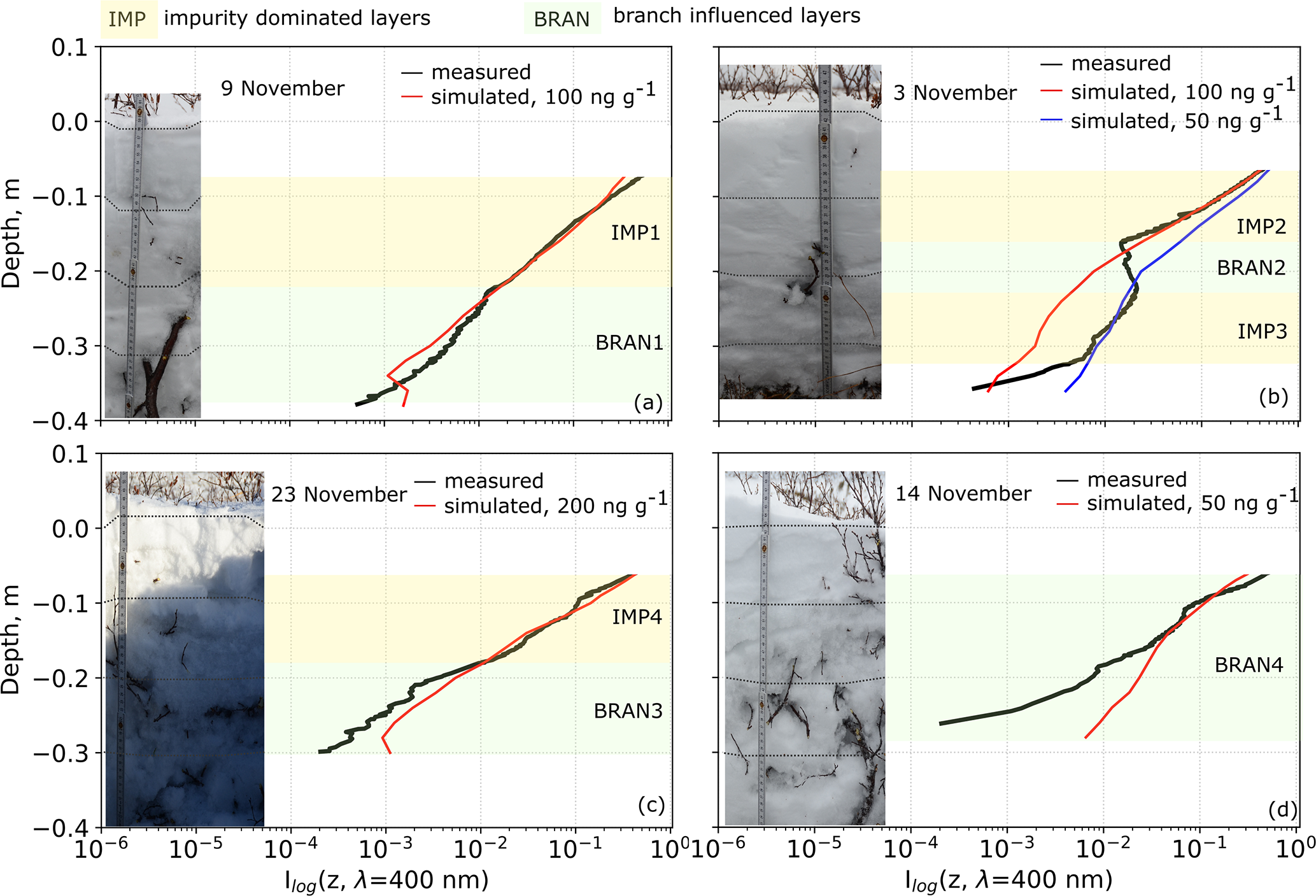
Figure 6 Log-irradiance and SnowMCML simulations at 400 nm for measurements taken on (a) 9 November, (b) 3 November, (c) 23 November and (d) 14 November in snowpacks with shrubs. Yellow shaded areas highlight layers where measured log-irradiance profiles and SnowMCML simulations fitted well. Green shaded areas highlight layers where log-irradiance and SnowMCML simulations fit less well and branches were visible in the snowpit photographs.

Unlike for the IMP layers, we found that for the second layer type (called BRAN1 through BRAN4) the log-irradiance profiles did not fit the SnowMCML simulations well. The log-irradiance profiles were also very irregular in comparison with IMP1 or IMP2, indicating a highly variable extinction coefficient. Finally, comparing the BRAN layers to the snowpit photographs revealed striking correspondences between these layers and the presence of branches. In Fig. 6a, a branch appeared at 22 cm depth, where the simulated and measured profiles start to diverge (BRAN1). Note that between snow depths 34 and 37 cm in BRAN1 the simulated profile shows a positive irradiance gradient which is not visible in the measured signal. As explained in Sect. 3.2 positive gradients can happen at transition zones and are an artefact caused by the rod. The discrepancy between the measured and modelled profiles arises most likely due to uncertainties in the measured snow physical properties input to the model. In Fig. 6b, two small twigs appeared between snow depths 16 to 24 cm, which coincided with a part of the log-irradiance profile that poorly fits the simulations (BRAN2). In this layer the measured profile shows a positive gradient but not the simulated profile. This discrepancy may again be caused by uncertainties in the snow physical properties, but it is more likely that here it is the result of the optical disturbance caused by branches. Branches absorb light locally, thus reducing the irradiance signal, but once the sensor exits the shadow of the branch, light may hit it from the side, resulting in an increase in measured irradiance and thus an enhancement of the positive gradient. This effect is not considered by the model, and the simulated profile therefore shows no increased irradiance. In Fig. 6c, the snowpit had generally more branches than the snowpits in Fig. 6a and b. Branches became particularly abundant between 10 and 40 cm depth, as also documented in our field notes. This was also where the simulation started to diverge more significantly from the measured profile (BRAN3). A high variability of the extinction coefficient, which was already observed in IMP4, was also visible in the irregular log-irradiance profile in BRAN3. Finally, in Fig. 6d, branches were abundant in the entire snowpit, and the measured profile could not be properly fitted to any of the simulations (BRAN4). BRAN4 also showed a highly variable extinction coefficient similar to the log-irradiance profile in Fig. 6c.

4.2.2 Spectral shape of k_{e_meas}(λ) vs. k_{e_calc}(λ)

We determined the k_{e_meas}(λ) and k_{e_calc}(λ) curves for the two different layer types identified with the SnowMCML method to test whether the optical differences are also visible in the spectral curves. The k_e analysis was performed for IMP1, IMP2 and IMP3 as well as for BRAN1 and BRAN4, but not for BRAN2, because k_e values were negative due to the observed positive extinction gradient, or for BRAN3 because the signal-to-noise ratio was too low. The results of the k_e analysis are shown in Fig. 7b. For comparison, we also show k_e curves for the ZOIs 1–3 in shrub-free snowpacks (Fig. 7a). For IMP2, k_{e_meas}(λ) and k_{e_calc}(λ) fitted very well (R²=0.98) in the 350–830 nm spectral range and returned BC concentrations of 95 ng g⁻¹, which concurs with the results from the SnowMCML simulations (BC = 100 ng g⁻¹). For IMP1 the fit was good for wavelengths <680 nm, and estimated BC concentrations (95 ng g⁻¹) concurred with SnowMCML results (BC = 100 ng g⁻¹). However, for wavelengths >680 nm the two curves started to diverge, and the k_{e_meas}(λ) curve showed a significant drop at wavelengths >780 nm, which did not appear in the theoretical k_{e_calc}(λ) curve. The same drop at longer wavelengths and the divergence between k_{e_meas}(λ) and k_{e_calc}(λ) curves was also observed in layers IMP3, BRAN1 and BRAN4. For those layers the fit between k_{e_meas}(λ) and k_{e_calc}(λ) was also generally lower with R² of −4.65 (IMP3), −9.32 (BRAN1) and 0.61 (BRAN4). Note the R² can be negative as it is not actually a square (Eq. 4). Negative R² indicates a poorly performing model (Motulsky and Christopoulos, 2003), which can happen when constraints are applied to a model. Here, we constrained the fit of k_{e_meas}(λ) and k_{e_calc}(λ) to the range 400–450 nm while performing model evaluation for a much larger range. The model used in the presented study is missing one component, i.e. the absorbing effect of branches, and it is thus not surprising that it has a poor fit. The misfit between model and measured data was intentionally used to study the effect of branches.

Figure 7 Measured and calculated k_e for (a) ZOIs in shrub-free snowpacks and (b) IMP and BRAN layers identified in snowpacks with shrubs (see also Fig. 6). Grey areas highlight the spectral range where calculated k_e was fitted to measured k_e. Deviations at wavelengths > 680 nm are interpreted as the influence of buried branches.

4.2.3 Radiative effect of buried branches

The results from the SnowMCML and k_e analysis suggest that in the two identified layer types, absorption profiles are either impurity-dominated (IMP1 to IMP4) or branch-influenced (BRAN1 to BRAN4). For the IMP layers there are several lines of evidence that suggest a BC-dominated absorption profile. First, log-irradiance profiles and SnowMCML simulations have a good fit, particularly in IMP1 and IMP2. Second, the measured log-irradiance profiles in IMP1 and IMP2 decrease linearly, indicating a constant extinction coefficient. These layers thus seem to have homogeneous optical properties and to be free of optical disturbances like branches. Finally, no branches were visible in the snowpit photographs. Therefore, it is reasonable to suggest that light absorption in the IMP layers was mostly dominated by BC concentrations, although the deviation between measurement and model k_e above 700 nm in IMP1 and IMP3 also indicates some influence of branches. In contrast, for the second layer type (BRAN1 through BRAN4, Fig. 6), snowpit images showed the presence of branches, log-irradiance profiles and SnowMCML simulations generally had a poorer fit than the IMP layers, and the measured log-irradiance profiles were visibly irregular, indicating high variability of the extinction coefficient. These irregularities are probably optical disturbances caused by branches. The irregularities may be caused through direct light absorption by branches, but also by branch shadows cast at the surface or within the snowpack. Especially during sunny conditions, the shadows cast by branches at the snow surface can have an impact on the quality of the irradiance profile with depth. The effect of shadows is attenuated with depth, while the area affected by the shadow increases. For example, a point shadow at the surface has a cone-shaped effect with depth, i.e. a circle that is extending with depth (with radius equal to depth). As a consequence, shadows cast by individual branches at the snow surface create a complex 3D field of light within the snowpack because the effects of the different shadows overlap. Thus, for a given point (x,y), the I(z) profile decreases and increases because of variations in the influence of different shadows and open areas, creating irregular profiles. Therefore, branch shadows could be one explanation for the irregular profile and variations observed in the extinction coefficient, particularly in BRAN3, which was measured on a sunny day.

The finding that shrubby snowpacks consist of two types of layers that are either impurity-dominated or branch-influenced was further corroborated by the spectral information from the k_e analysis. IMP2 is the best example for an impurity-dominated layer where absorption properties of BC were well suited to reproduce the observed spectral extinction. In contrast, for IMP1, IMP3, BRAN1 and BRAN 4 the k_{e_meas}(λ) curves displayed a drop at wavelengths >680 nm, which was not visible in the k_{e_calc}(λ) curves. We interpret this drop as a strong indicator of the influence of branches (Fig. 7), because reflectivity measurements for Arctic shrub branches showed that branches are highly absorbing at 400–500 nm but that reflectivity increases slightly at 500 nm and then even more sharply at 680 nm (Juszak et al., 2014) (Fig. 1). Thus, the optical properties of branches seem well suited to explain the observed drop in extinction at 500–900 nm in the measured k_e curves (Fig. 7). In contrast, k_{e_calc}(λ) curves were calculated assuming that all the extinction other than by snow or the rod was due to BC. In this case, the k_{e_calc}(λ) curves overestimate extinction in the spectrum >500 nm because in this range BC is more absorbing than branches. It is likely that in IMP1 and IMP3 branches had some influence on the irradiance profile, although the measured log-irradiance fitted well with the SnowMCML simulations, and no branches were detected in the photographs. In BRAN1 to BRAN4 the effect of branches seemed to be stronger, as suggested by the multiple indicators for branch influence (for example irregular profiles or the mismatch between measured log-irradiance and SnowMCML simulations). In contrast, almost no influence of shrubs could be detected in IMP2 despite the layer being located in a snowpack with shrubs. This leads us to conclude that the optical effect of a buried branch must be highly localized and that its impact strongly weakens as a function of distance from the branch. The log-irradiance profiles here were measured at different distances to branches, but the exact distances are unknown to us, which is why the strength of the influence of branches varied in the different IMP and BRAN layers. This shows that quantifying the impact of branches would require knowing the position of branches in the snowpack with precision, making the task of quantifying the effect of buried branches more complex. Moreover, the magnitude of the radiative effect of branches also varies as a function of wavelength, as indicated by the results from the k_e analysis where branches, compared to BC, reduce the absorption coefficient at 700 nm by 2 to 12 m⁻¹ and at 800 nm by 12 to 27 m⁻¹.

4.2.4 Local heating effect and impact on snow physical properties

An important consequence of light absorption by buried branches is a local heating effect. This local heating assumption was mentioned in Sturm et al. (2005) and Pomeroy et al. (2006) and is further supported by cursory observations on snow physical properties made during the field campaign in this study. During a warm spell on 19 and 20 November 2015, we observed that snow melt rates were increased in the direct vicinity of branches, forming a snowpack filled with holes (Fig. 8a and b). If shrub-induced radiative heating had had a non-local effect, the snowpack would have melt more homogeneously than the observed Swiss-cheese-looking snowpack. Localized melting around buried branches was also suggested by Sturm et al. (2005) and Pomeroy et al. (2006), which they considered to be an important factor for shrub spring-up in spring. In addition to the melt holes, we also found large clusters of melt–freeze grains attached to branches (Fig. 8c and d), indicating local melting. A non-local effect could be caused during warm spells in autumn and in spring, when more extensive melting may be possible, leading to percolation that would affect the whole snowpack, but this was not observed. When conditions were cold enough to prevent melting, the local radiative heating effect of branches resulted in the formation of pockets of depth hoar (or faceted crystals) around branches (Fig. 8e and f). Depth hoar are snow grains with a high metamorphic degree (Akitaya, 1975) and are formed by high water vapour fluxes generated by strong temperature gradients in snowpacks. Strong vertical temperature gradients exist in the Arctic tundra in autumn, between the cold atmosphere and the relatively warmer soils. In the absence of shrubs, these temperature gradients typically form horizontal layers of depth hoar at the bottom of the Arctic snowpack. In the presence of shrubs, temperature gradients between the warmer branches and the colder snow nearby are increased, leading to enhanced depth hoar formation. As the effect of branches is very local, however, this causes metamorphism only in the direct vicinity of branches, explaining the formation of depth hoar pockets rather than layers. This effect is particularly important for branches near the surface due to the proximity with the cold atmosphere and the higher irradiance. However, when depth hoar starts forming, its low thermal conductivity increases thermal gradients and further favours depth hoar formation so that the process may persist near branches even once they are deeply buried (this is also discussed in Domine et al., 2016). The effect of branches on melting and depth hoar formation may vary in different topographical settings because microtopography impacts total snow accumulation but also snow density, with wind-exposed areas having denser snowpacks than wind-sheltered areas. However, topography was similar in all our sites so no topography-induced impact could be studied.

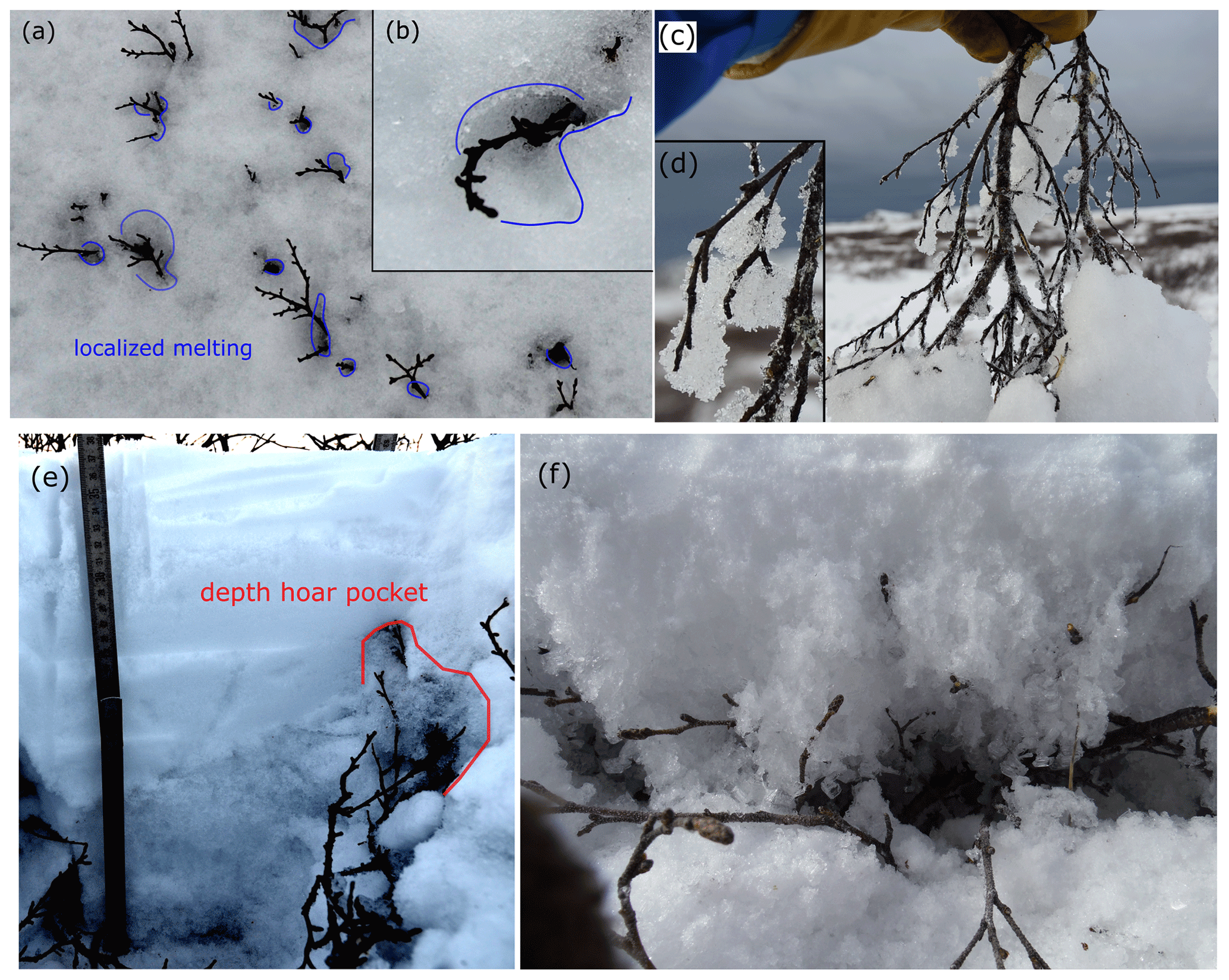
Figure 8 Photos showing observations of localized snow melting around branches (a, b), a branch cut from a buried shrub with attached clusters of melt–freeze grains (c, d) and the formation of depth hoar pockets around buried branches (e, f). Photos were taken during the measurement campaign from 29 October to 6 December 2015. In (e) the contrast of the photo was increased to better reveal the depth hoar pockets.

The modifications of snow physical properties induced by buried branches are important because they influence the insulating effect of snow. In particular, depth hoar layers have very good insulating properties (Domine et al., 2016), while melt–freeze layers are poor insulators (Barrere et al., 2018). The insulating properties of a snowpack are critical for the survival of Arctic flora and fauna in winter (Berteaux et al., 2017; Domine et al., 2018) and directly impact the thermal regime of permafrost, which has important implications for ongoing climate change (Koven et al., 2013; Schuur et al., 2015). Apart from these ecosystem-related consequences, shrub-induced modifications of snow physical properties are also disturbing the layered structure of the snowpack which is important for radiative transfer models calculating light propagation through snow under the presumption that snowpacks are plane-parallel media. It may be important to factor in these branch-induced structural disturbances in future studies simulating snow radiative transfer in mixed snowpacks.

4.3 Source of high BC concentrations

The data presented here on shrub-free snowpacks were not intended to be an exhaustive study of impurities in snow in the Umiujaq region, as their primary objective was to serve as a comparison to the measurements in snowpacks with shrubs. It is nevertheless noteworthy that BC concentrations measured on 8 and 22 November were unexpectedly more than twice as high as the median values reported for the rest of the Arctic, where concentrations outside Greenland lie around 20 ng g⁻¹, with slightly higher values up to 60 ng g⁻¹ in Arctic Russia and Scandinavia (Doherty et al., 2010). High values similar to those measured here usually occur in mid-latitudes, for example in northern China (117–1220 ng g⁻¹) (Wang et al., 2013) or the Chilean Andes (up to 100 ng g⁻¹) (Rowe et al., 2019), where the proximity to cities and industrial activities produces more BC. The Arctic was usually found to be cleaner due to its distance to BC source regions (Skiles et al., 2016) and because BC concentrations have been continuously declining since industrial BC emissions in Europe and North America started decreasing in the early twentieth century (McConnell et al., 2007; Gong et al., 2010).

The high BC concentrations this study determined in Umiujaq cannot be due to forest fires because they do not happen in late autumn or winter and are therefore most likely due to local anthropogenic sources early in the snow season. These could be snowmobile traffic in the valley and, perhaps more importantly, the waste burning occurring ∼ 2 km upwind from our study site (Fig. 2). Such local anthropogenic sources in the Arctic may become more influential as Arctic tourism keeps blooming, ship traffic keeps increasing and northern communities keep growing. It is thus most likely that the contribution of BC emissions produced in the north, amongst others by waste burning, will increase in the near future. This is important because BC in snow has a significant impact on snow albedo. Models have calculated that at concentrations in the 5–50 ng g⁻¹ range BC reduces albedo by up to 4 %. Albedo reductions of 4 % can cause positive radiative forcing of up to 16 W m⁻² during an average Arctic spring and early summer day and hence are climatically significant (Warren, 2019b). Moreover, decreases in snow albedo can possibly advance the melt season by a few weeks (Tuzet et al., 2020), causing extensive environmental perturbations, and also amplify the impact of warm spells in autumn. However, more research is necessary to accurately quantify BC production in Umiujaq and in northern communities in general and to determine potential impacts. Nevertheless, our findings highlight that the anthropogenic footprint in the Arctic may be important and suggest that a cleaner waste management should be considered for the self-protection of northern communities and the ecosystem.

5 Conclusions

This study presented the first measurements of irradiance profiles in snowpacks with shrubs, together with comparative irradiance measurements acquired in shrub-free snowpacks. Irradiance profiles measured in snowpacks with shrubs showed that the impact of branches was local. In some layers, light absorption depended primarily on BC concentrations, and branches played only a minor role. In other layers, coinciding with where branches were visible in snowpit photographs, the branch effect was more prominent, suggesting the local-effect hypothesis. This assumption was further supported by cursory observations of localized melting and depth hoar pockets forming in the vicinity of branches in the snowpack. The local modification of snow physical properties by branches and the resulting changes in snow microstructure impact the insulating properties of snow with potential consequences for Arctic flora and fauna as well as the thermal regime of permafrost. Moreover, the branch-induced modifications in snow physical properties increase the heterogeneity of the snowpack and disturb its plane-parallel structure. The structural changes are important for measuring or modelling the radiative impact of shrubs and should be considered by future research.

Profiles measured in shrub-free snow were analyzed to determine impurity types and concentrations. For snow in Umiujaq, the main impurity, as inverted from a radiative transfer model, was black carbon (BC), which occurred in concentrations with large spatiotemporal variability. Some layers featured low concentrations (8 ng g⁻¹) while other layers had concentrations as high as 185 ng g⁻¹. High concentrations were likely caused by the emission of nearby open-air waste burning. The high BC concentrations reported here may be one of the first indicators that cleaner waste management plans are required to avoid the production of important BC concentrations from local sources in the Arctic. Impurities in Arctic snow accelerate snow melting in spring and can also amplify the impact of warm spells in autumn. Based on our results and given the important impact impurities can have on snowmelt timing, we suggest further research on the regional and long-term importance of waste management in Arctic regions.