the Creative Commons Attribution 4.0 License.
the Creative Commons Attribution 4.0 License.
 | 30 Nov 2021
Enhanced chlorophyll-a concentration in the wake of Sable Island, eastern Canada, revealed by two decades of satellite observations: a response to grey seal population dynamics?
Emmanuel Devred
Andrea Hilborn
Cornelia Elizabeth den Heyer
Elevated surface chlorophyll-a (chl-a) concentration ([chl-a]), an index of phytoplankton biomass, has been previously observed and documented by remote sensing in the waters to the southwest of Sable Island (SI) on the Scotian Shelf in eastern Canada. Here, we present an analysis of this phenomenon using a 21-year time series of satellite-derived [chl-a], paired with information on the particle backscattering coefficient at 443 nm (bbp(443), a proxy for particle suspension) and the detritus/gelbstoff absorption coefficient at 443 nm (adg(443), a proxy to differentiate water masses and presence of dissolved organic matter) in an attempt to explain some possible mechanisms that lead to the increase in surface biomass in the surroundings of SI. We compared the seasonal cycle, 8 d climatology and seasonal trends of surface waters near SI to two control regions located both upstream and downstream of the island, away from terrigenous inputs. Application of the self-organising map (SOM) approach to the time series of satellite-derived [chl-a] over the Scotian Shelf revealed the annual spatio-temporal patterns around SI and, in particular, persistently high phytoplankton biomass during winter and spring in the leeward side of SI, a phenomenon that was not observed in the control boxes. In the vicinity of SI, a significant increase in [chl-a] and adg(443) during the winter months occurred at a rate twice that of the ones observed in the control boxes, while no significant trends were found for the other seasons. In addition to the increase in [chl-a] and adg(443) within the plume southwest of SI, the surface area of the plume itself expanded by a factor of 5 over the last 21 years. While the island mass effect (IME) explained the enhanced biomass around SI, we hypothesised that the large increase in [chl-a] over the last 21 years was partly due to an injection of nutrients by the island's grey seal colony, which has increased by 200 % during the same period. This contribution of nutrients from seals may sustain high phytoplankton biomass at a time of year when it is usually low following the fall bloom. A conceptual model was developed to estimate the standing stock of chl-a that can be sustained by the release of nitrogen (N) by seals. Comparison between satellite observations and model simulations showed a good temporal agreement between the increased abundance of seal on SI during the breeding season and the phytoplankton biomass increase during the winter. We found that about 20 % of chl-a standing stock increase over the last 21 years could be due to seal N fertilisation, the remaining being explained by climate forcing and oceanographic processes. Although without in situ measurements for ground truthing, the satellite data analysis provided evidence of the impact of marine mammals on lower trophic levels through a fertilisation mechanism that is coupled with the IME with potential implications for conservation and fisheries.
- Article
(8219 KB) - Full-text XML
- BibTeX
- EndNote


Increased phytoplankton production around islands, known as the island mass effect (IME), has been documented in many studies since the development of the concept (Doty and Oguri, 1956). This phenomenon, often occurring leeward of islands, results from a large range of processes, among which are mixing of the water column induced by hydrodynamic forcing (e.g., flow disturbance), benthic resuspension (Signorini et al., 1999) and land drainage (Dandonneau and Charpy, 1985) that provide nutrients to the well-lit upper layer of the ocean (Heywood et al., 1990), in turn sustaining enhanced phytoplankton production (e.g., Gilmartin and Revelante, 1974; Gove et al., 2016; Messié et al., 2020; James et al., 2020). Evidence of the IME has been documented in the proximity of islands located in oligotrophic oceanic basins (Dandonneau and Charpy, 1985; Gove et al., 2016; Messié et al., 2020) and in mesotrophic and sub-Antarctic environments (Boden, 1988). Ocean colour remote sensing (OCRS) has proven to be a useful tool to observe increased primary production around islands and study its spatio-temporal variation given the fine spatial and temporal scales achievable in comparison to in situ sampling (e.g., Signorini et al., 1999; Gove et al., 2016; Martinez et al., 2018; Martinez and Maamaatuaiahutapu, 2004; James et al., 2020). For the first time, to our knowledge, IME around an island located in the mesotrophic environment of the eastern Canadian continental shelf, Sable Island (SI), is investigated using OCRS. The Scotian Shelf is a productive environment with an annual mean chlorophyll-a concentration ([chl-a]) of about 0.75 mg m−3 (± 0.38 mg m−3) observed by ocean colour satellites. Phytoplankton biomass is subject to a strong seasonal cycle, with a spring bloom representing a major food input into the ecosystem and a secondary fall bloom triggered by the replenishment of nutrients to the surface-lit layer as a result of physical forcing (Song et al., 2010). While this general progression is well established, the mesoscale patterns of phytoplankton dynamics are more complex given the complicated bathymetry and hydrodynamics of the Scotian Shelf. For instance, the effect of the numerous banks and channels results in spatially distinct timing and intensities of the spring bloom throughout the surface waters of the shelf (Casault et al., 2020) and an overall patchiness in phytoplankton growth and decay (Denman and Platt, 1976). However, a feature that remains constant is the moderate to high surface phytoplankton biomass that occurs leeward of SI in comparison to its surroundings as observed by satellite OCRS (Fig. 1). While this has been documented in previous studies (King et al., 2016; Zhai et al., 2011), the temporal and spatial dynamics of this plume off SI have not been examined using a 21-year time series of satellite records. We further discuss possible mechanisms that explain the high phytoplankton biomass, and, in particular, we consider a previously neglected source of nutrient entrainment into the local ocean; the presence of the world's largest colony of grey seals (Halichoerus grypus). The breeding colony on SI has grown rapidly since the 1960s when just a few thousand pups were born on the island (Bowen et al., 2007; den Heyer et al., 2020). The population associated with the SI breeding colony is now over 300 000 individuals (Rossi et al., 2021), and the impact of this population on prey species has been focus of much research (e.g., Trzcinski et al., 2006; O'Boyle and Sinclair, 2012; Hammill et al., 2014; Neuenhoff et al., 2019). Recently the grey seal breeding colony has also been shown to contribute to the ecology of the island by fertilising vegetation that supports a population of feral horses (McLoughlin et al., 2016). Previous studies have demonstrated the impact of marine mammals on the supply of nutrients by direct release of N in the marine environment (Roman and McCarthy, 2010; Laver et al., 2012; Mccauley et al., 2012; Wing et al., 2014), through turbulent mixing (Kanwisher and Ridgway, 1983) and atmospheric deposition (Theobald et al., 2006).
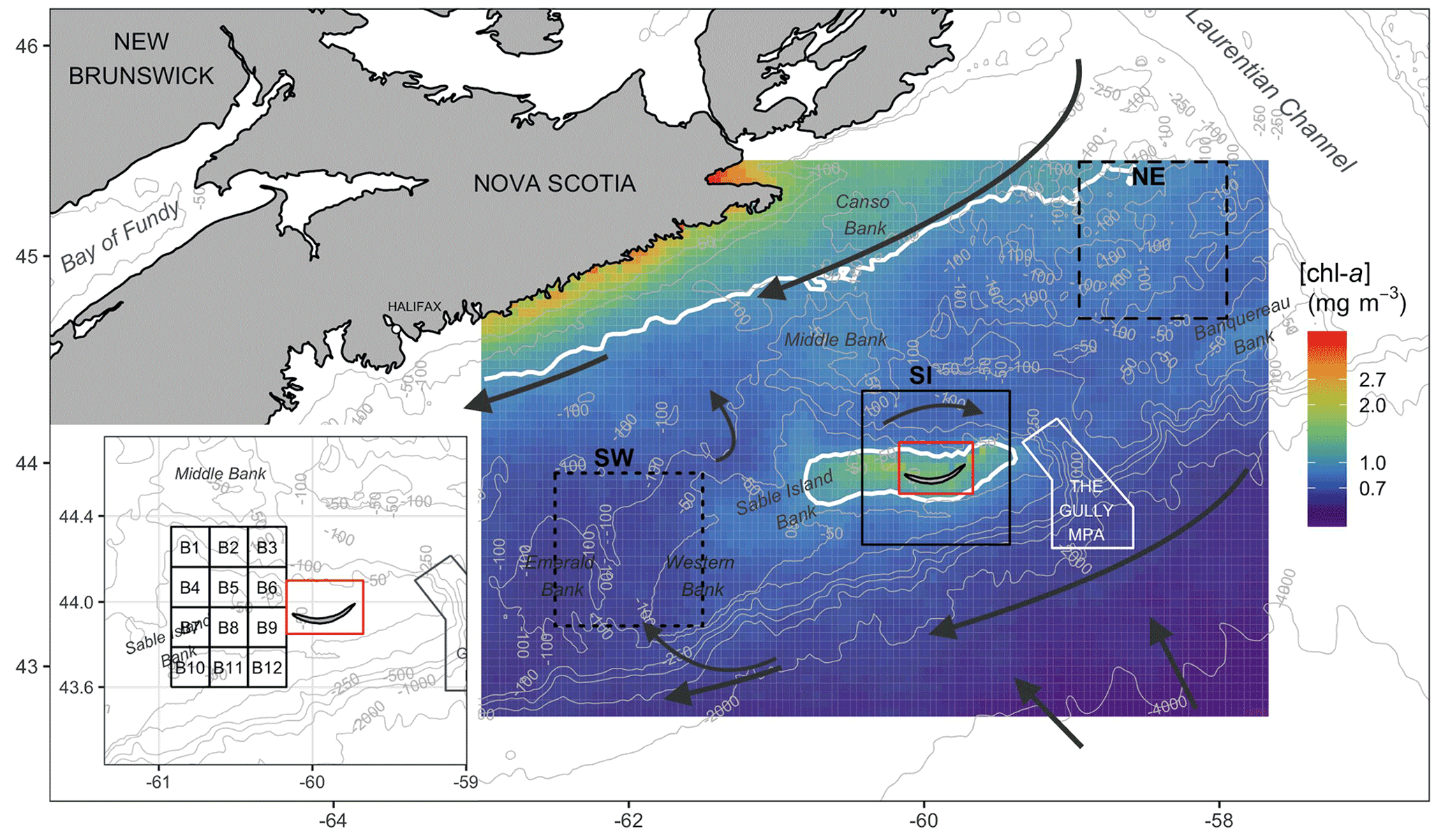
Figure 1Map of the Scotian Shelf showing bathymetric features (grey lines), main hydrodynamic circulation (dark arrows) and the three regions used for analysis (solid black line is SI; short-dashed line is the southwest, SW; and long-dashed line is the northeast, NE). Pixels in the red box were removed from analysis. The inset shows 12 small boxes adjacent to SI (see Sect. 2.4). The mean [chl-a] over the period 1998–2018 is shown in the background, with white contours delineating 1.0 mg m−3.
The Ocean Colour Climate Change Initiative (OC-CCI) satellite time series over the period 1998–2018 was used to investigate the dynamics of [chl-a] (in mg m−3), absorption by detritus and dissolved organic matter (DOM, adg(443) in m−1), and the backscattering coefficient (bbp(443) in m−1) around SI and over a portion of the Scotian Shelf. In addition to [chl-a], we considered variations in absorption by yellow substances and detritus to help track possible runoff from the island and significant sources of dissolved organic matter, while variations in the backscattering coefficient were used to indicate the presence of mineral particles in the water column (Boss et al., 2004; Slade and Boss, 2015) near the island due to resuspension as both of these properties could induce an artificial increase in [chl-a] observed by satellite (Bukata et al., 1995). The first objective of the study was to demonstrate and quantify the higher phytoplankton biomass around SI and evidence the IME. Given that the time series of satellite observations span over two decades, we analysed the 8 d climatologies and seasonal cycles of several subregions of the Scotian Shelf, including SI, using the artificial neural network technique of self-organising maps (SOMs) to isolate recurring patterns of [chl-a], and we investigated decadal trends of the three remote-sensing parameters. While the information provided by satellites remains limited to marine components that are optically active, the second objective of the study was to examine some of the possible mechanisms causing such an increase in biomass in space and time around the island, and in particular fertilisation by seal excretion. The first part of the paper presents the area of interest, data and methodology, with the results and discussion section organised to answer the following questions.
-
Is there an IME, and if so, what is its spatio-temporal distribution?
-
Are there decadal trends in the satellite-derived properties around SI?
-
What is(are) the possible mechanism(s) that can explain the trends?
2.1 Study area
The Scotian Shelf bioregion is a significant marine shelf region due to its biological richness and diversity (Ward-Paige and Bundy, 2016). The influence of the warm gulf stream makes the area home to marine species normally found further south, and it is used as spawning and nursery grounds by many fish species. The mean surface circulation consists of a persistent current flowing to the southwest, trapped by the coast, and a parallel cold current (Labrador Current) flowing to the southwest along the shelf break (Smith and Schwing, 1991; Loder et al., 1997) (Fig. 1). The Scotian Shelf is bounded to the east by the Laurentian Channel, to the west by the Northeast Channel and to the south by the continental shelf break oriented parallel to coastal Nova Scotia. SI is the only island on the shelf, emerging centrally adjacent to the shelf break from Sable Island Bank (SI Bank; see Fig. 1); most of the bank is an ecologically and biologically significant area (EBSA) due to its high abundance of groundfish and persistently high [chl-a] (King et al., 2016). While the average depth of the Scotian Shelf is 90 m, there is complex circulation over banks and basins as deep as 300 m, and SI Bank lies at a depth of approximately 60 m. SI itself has a surface area of only 34 km2 (about 49 km in length with large interannual variation and 1.25 km at its widest point) and is composed of sand and partially vegetated by marram grass (Ammophila breviligulata), other grasses, forbs, and shrubs and as a result undergoes little surface runoff. Precipitation directly recharges a freshwater aquifer that runs the length of the island maintained by hydrostatic pressure (Kennedy et al., 2014). SI is home to a population of feral horses in addition to hosting the largest breeding colony of grey seals (Halichoerus grypus) in the northwest Atlantic that aggregate in breeding colonies from December to February.
While the focus of this study is the marine region adjacent to SI, data were also analysed for two control boxes, which were arbitrarily selected near the island to evidence the unique increase in biomass around SI (Fig. 1) and to ensure that the findings around SI were the results of local processes and not only the reflection of a general pattern occurring over the entire Scotian Shelf. One box was located to the northeast (i.e., upstream and referred to as NE with a mean depth of 111 m) and the second one was located to the southwest (downstream and referred to as SW with a mean depth of 83 m) of SI. These boxes were located far enough from SI and the continent to avoid influences of terrigenous runoff. A large box centred on SI of the same geographic size to NE and SW was defined to investigate the possible IME, and a grid made up of 12 small boxes to the west of the island was defined to infer the spatial extension of the SI plume (Fig. 1, inset) without subjective delineation.
2.2 Satellite and environmental datasets
Satellite data were downloaded from the Ocean Colour Climate Change Initiative (OC-CCI, https://rsg.pml.ac.uk/thredds/catalog-cci.html, last access: 15 November 2021), a project providing validated, inter-sensor calibrated and error-characterised Essential Climate Variables (ECVs) from several satellite sensors (OC-CCI dataset v4.0; Sathyendranath et al., 2019, 2020). The dataset consists of merged products from the Sea-viewing Wide Field-of-view Sensor (SeaWiFS, 1997–2010), MEdium Resolution Imaging Spectrometer (MERIS, 2002–2012), Moderate resolution Imaging Spectroradiometer on Aqua satellite (MODISA, 2002–present) and Visible Infrared Imaging Radiometer Suite sensors (VIIRS, 2012–present). For this study, 8 d 4 km resolution composites of [chl-a], adg(443) and bbp(443) were extracted from the global dataset for a region bounded by 42.7–45.45∘ N and 57.6–63.0∘ W. The [chl-a] was produced by the OC-CCI from remote-sensing reflectance (Rrs) using the OC3 algorithm (see Jackson et al., 2020, for details), dependent on water class membership, where Rrs values are atmospherically corrected using the SeaWiFS Data Analysis System (SeaDAS 7.3) and POLYMER software (Steinmetz et al., 2011). Inherent optical properties (IOPs) such as adg(443) and bbp(443) are calculated at SeaWiFS wavelengths from Rrs using the quasi-analytical algorithm (Lee et al., 2005). For the SI box, a small rectangle containing the island and submerged shallows was masked from all calculations (shown as the red box in Fig. 1) to reduce the impact of pixels potentially influenced by resuspended sediment or bottom reflectance. Further, large coccolithophore blooms occasionally occur in the surrounding waters of SI (Moore et al., 2012), which increases the magnitude of bbp(443), as the white skeleton of coccolithophores (i.e., coccoliths), made of calcite, has strong scattering properties. Therefore, 8 d composite images with bbp(443) several orders of magnitude greater than the annual mean in a given year were discarded to remove the impact of high scattering coefficients due to the presence of coccolithophore blooms. This included the periods of 25 June through 11 August 2003 and 25 June through 3 August 2010. Lastly, 24 images with erroneous data were identified and removed during the SOM processing (see Sect. 2.4). The resulting remote-sensing dataset used in this study consisted of 958 [chl-a] and adg(443) and 946 bbp(443) level 3 8 d composites spanning from 1998 to 2018.
The 5 d composite NASA OSCAR sea-surface velocity dataset (https://data.noaa.gov/dataset/dataset/oscar-sea-surface-velocity-1-3-l4-global-1992-present-5-day-composite1, last access: 15 November 2021) at ∘ resolution was downloaded from the NOAA ERDDAP server (https://coastwatch.pfeg.noaa.gov/erddap, last access: 15 November 2021, dataset ID: jplOscar_LonPM180) for the corresponding time period to the satellite observations. The zonal (u in m s−1) and meridional (v in m s−1) components of the sea-surface velocity field were further averaged into monthly and annual fields to examine prevailing current speed and direction. We also examined the meteorological data over the period 1998–2018, including daily wind speed and precipitation, from an Environment and Climate Change Canada station located on SI (ID 8204700, https://climate-change.canada.ca/climate-data/#/daily-climate-data, last access: 15 November 2021). Bathymetry was acquired from NOAA ETOPO1 and used to calculate chl-a standing stocks (Sect. 2.5.2).
All analyses were performed using R statistical software (R Core Team, 2020).
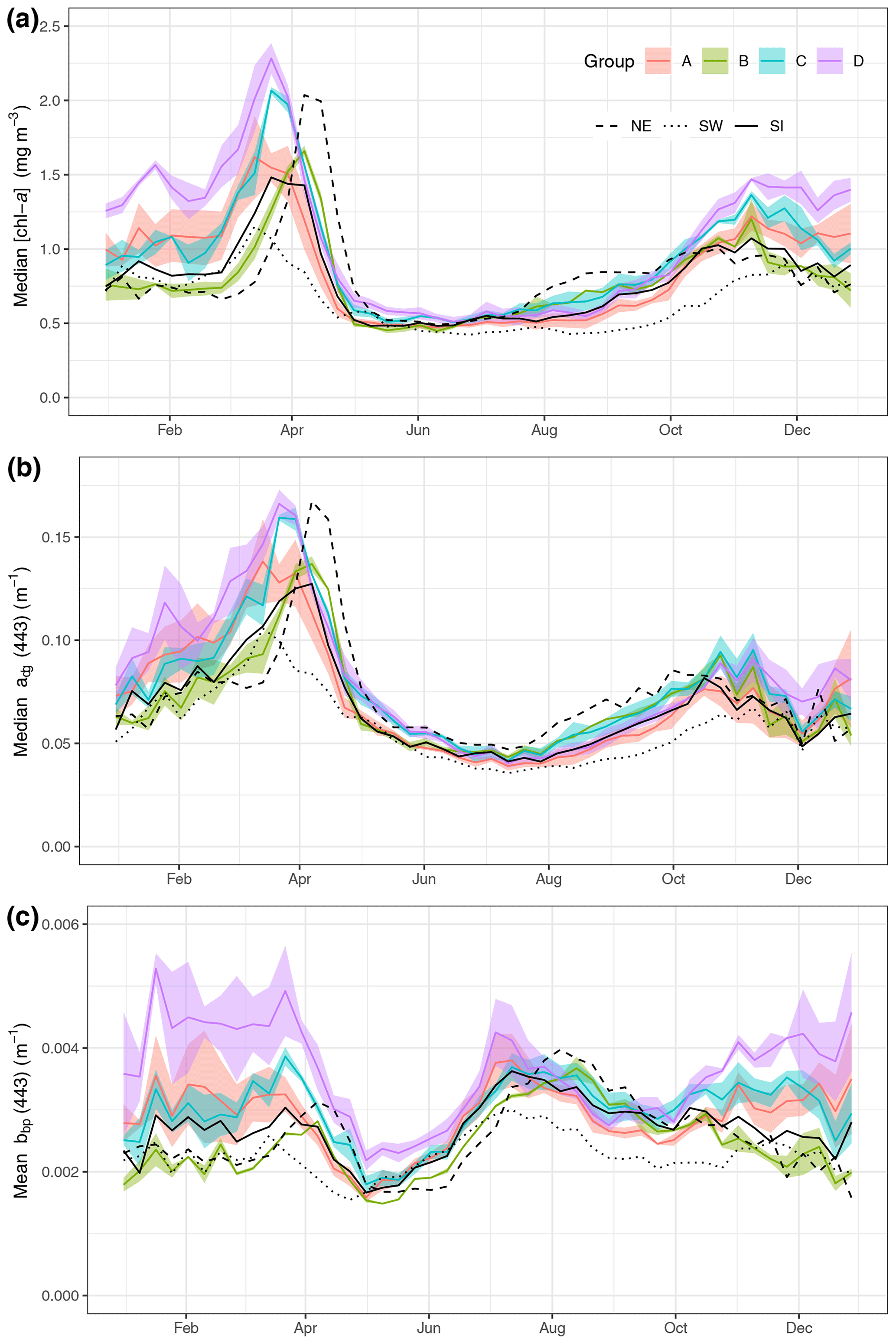
Figure 2Median value per week of [chl-a] (a), adg(443) (b) and bbp(443) (c) for the regions on the Scotian Shelf (see Fig. 1). The three large regions are noted by black lines (SW is dotted, SI is solid and NE is dashed). The coloured line represents means of small boxes with similar seasonal cycles; groups A, B, C and D correspond to boxes 1 to 3, 4 to 6, 7 to 9 and 10 to 12, respectively.
2.3 Eight-day climatology and trends of satellite [chl-a], adg(443) and bbp(443)
Eight-day climatologies of [chl-a], adg(443) and bbp(443) for SI and the two control boxes (i.e., SW and NE) were calculated as the average of all pixels of all years within a given 8 d period and box (Fig. 2). Pixels with values outside of the 1.5 interquartile range (IQR) were removed, and, following that step, boxes with less than 30 % of spatial coverage for a given 8 d period were discarded to ensure the highest quality of the data and prevent skewing of results by outliers. In addition, 8 d climatologies were computed for a total of 30 small boxes (0.2∘ × 0.2∘) organised around SI to identify in an objective manner the region of influence of the IME. A total of 18 small boxes, located north and east of the island, were not used for further analysis because they showed a similar [chl-a] 8 d climatology to the control boxes, meaning that they were not subjected to the IME. The analysis focused on the 12 remaining boxes to help understand and quantify the variability in [chl-a], adg(443) and bbp(443) southwestward of SI (Fig. 1, inset). Finally, the boxes with similar temporal patterns were averaged together for clarity and referred to group A for boxes 1, 2, 3 and 4; group B for boxes 5 and 6; group C for boxes 7, 8 and 9; and group D for boxes 10 to 12.
In addition to the 8 d time binning, seasonal composites of [chl-a], adg(443) and bbp(443) were computed as the arithmetic mean of images during winter, spring, summer and fall for the SW and NE boxes, as well as a plume defined by [chl-a] greater than 1 mg m−3 located southwest of SI and occurring in the winter (i.e., SOM5; see Sect. 2.4 for details). Winter, spring, summer and fall were defined as the months of December to February, March to May, June to August, and September to November, respectively. The same quality control used for the 8 d climatology calculations was also implemented. The seasonal binning was favoured against the 8 d composite for the trend analysis as it decreased the impact of missing data in the time series, allowing a better definition of the chl-a plume. The seasonal long-term trends were computed as the slope of the linear least-squares regression for [chl-a], adg(443) and bbp(443) against time.
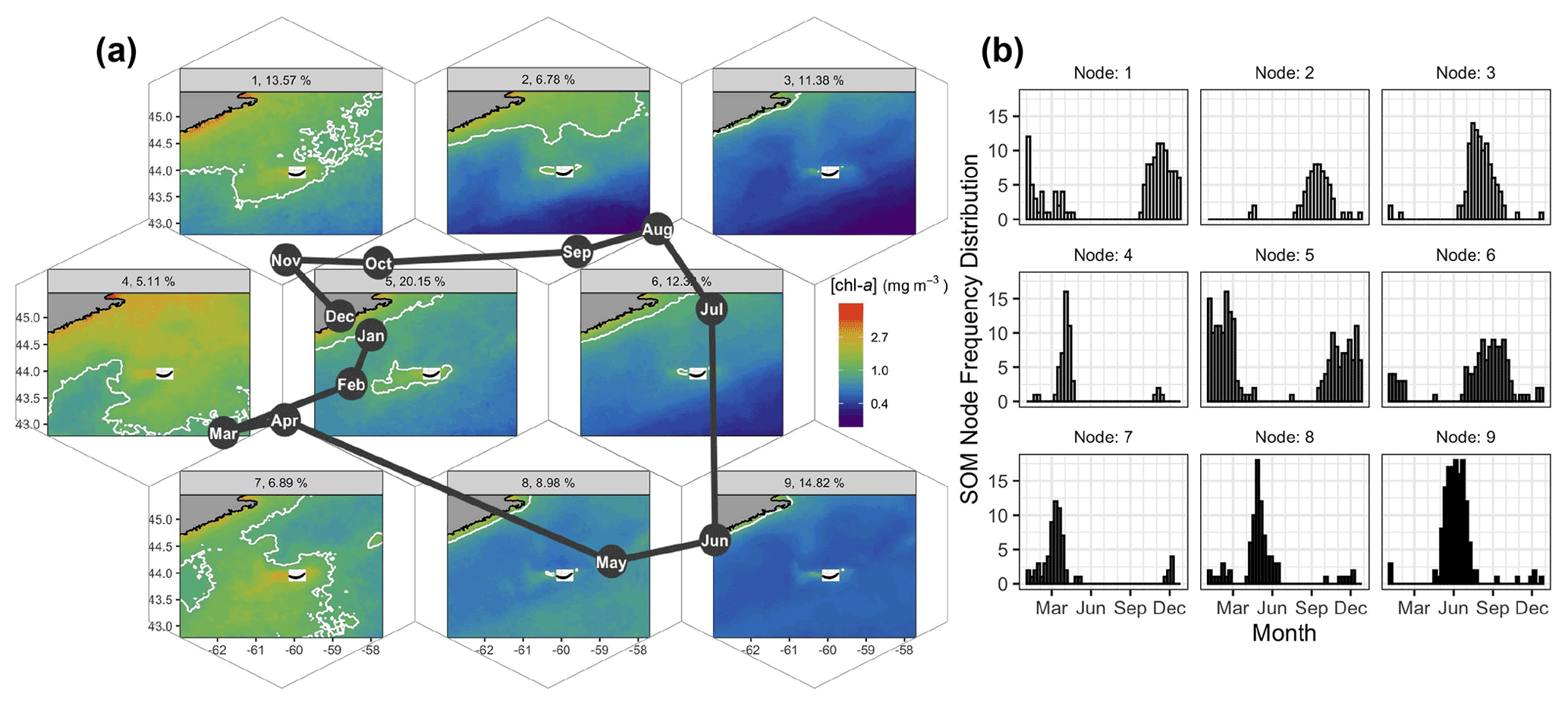
Figure 3Results of the SOM shown hexagonally to illustrate the spatial structure of [chl-a] in the SOM layout as well as their annual succession (a). The node number and percent occurrence in the time series are shown in the light grey banner on top of each pattern of [chl-a]. The solid white contour delineates 1.0 mg m−3. The month abbreviations in the dark solid circles represent the most occurrence of each SOM node. For instance, node no. 8 occurred mainly in May, and about 9 % of the 8 d images were associated with that node. The number of 8 d composite images per node and per month are shown as histograms on the right panel (b).
While the above time series and trend analysis are useful to quantify changes in the bio-optical properties around SI, we selected a different approach to bin the satellite data for comparison with model simulations (see Sect. 2.5.2). The satellite data were averaged into 5-year time periods, namely, 1999–2003 (P1), 2004–2008 (P2), 2009–2013 (P3) and 2014–2018 (P4), to reduce the impact of missing data in the maps of [chl-a] for the SOM5 region. Note that the year 1998 was discarded from this analysis to have all periods equal to 5 years exactly. These maps were used to calculate chl-a standing stocks from ocean colour satellite for comparison with chl-a standing stocks derived from seal N excretion (see Sect. 2.5.2). The chl-a standing stocks independent of possible seal influence during P1 were computed by subtracting the chl-a standing stocks due to seal N excretion from the satellite observations and referred to as P1N. This initial value was linearly extrapolated to the three other periods (i.e., P2, P3 and P4) by applying the slope of the [chl-a] linear trends derived in the SW box, which is assumed to be too far from the island to be influenced by seal fertilisation. The P2N, P3N and P4N chl-a standing stocks obtained using this method provided the increase in chl-a standing stocks due to physical processes without any influence from the presence of seals on SI. Note that in November of 2011, an unusual and intense phytoplankton bloom occurred southward of SI, partially covering the SOM5 region but not connected to SI; this bloom that lasted almost the entire month was removed from the analysis as it contaminated the background [chl-a] and was not part of the IME.
2.4 Chlorophyll-a concentration spatio-temporal variation using self-organising maps (SOMs)
Self-organising maps (SOMs) are a useful tool for extracting patterns in time series of satellite imagery and their frequency of occurrence (Richardson et al., 2003), with previous applications including pattern analysis of sea-surface height (Hardman-Mountford et al., 2003), spatio-temporal scatterometer and sea-surface temperature (SST) variation (Richardson et al., 2003), and improved pixel classifications of satellite [chl-a] time series (Ainsworth, 1999). Here we applied the SOMs method to the satellite [chl-a] estimates to summarise the spatio-temporal dynamics of phytoplankton biomass. The basic principle of a SOM is to map high-dimension data, in our case a three-dimensional dataset (i.e., two dimensions in space and one in time), to a two-dimensional array of nodes. The kohonen R package (Wehrens and Buydens, 2007; Wehrens and Kruisselbrink, 2018) was applied as an unsupervised SOM method to the 21-year dataset of OC-CCI [chl-a] for a region bounded by −63 to −57.5∘ E and 42.8 to 45.5∘ N (Fig. 3). Nine nodes were selected after trials of multiple layout configurations, as it provided low mean node distance and enough nodes to represent distinct spatial patterns of [chl-a] and avoid redundancy, with each node accounting for a distinct general pattern across the time series (Fig. 3a). Each 8 d image retained a measure of fit (i.e., resemblance) to the node it was assigned to (referred to as distance), with a large distance indicating a poor membership of a given 8 d image to a node. The final result had each node (i.e., [chl-a] map) representing a particular spatial pattern consisting of the distance-weighted average of its assigned images, with similar nodes located nearer each other in the final SOM layout (Fig. 3a). This is an iterative procedure that runs until the overall distance of the entire system is minimum; in this case, a total of 500 iterations was sufficient for the mean distance of all nodes to converge and for all individual node distances to stabilise to a similar value (0.0042, unitless). Note that prior to processing, the daily [chl-a] images were log-transformed, and images with less than 10 % spatial coverage were excluded from the analysis. Temporal gaps were not accounted for, as images are assigned to the node array individually with no dependence on position in the time series. A total of 24 [chl-a] images were identified as having persistently high node distance through all trials (e.g., did not fit with any node, regardless of array size), which when visually inspected displayed heterogeneous and often unrealistic [chl-a] values (e.g., very high); these images and corresponding adg(443) and bbp(443) were removed from the dataset for all analysis including the SOM, 8 d climatology computation and time series analysis. The temporal occurrence of each node in the 21-year time series was recorded for each month to produce frequency histograms (Fig. 3b) as in Richardson et al. (2003). Additionally, given that we are interested in the elevated [chl-a] near SI in winter, the SOM results were used to delineate a plume where [chl-a] exceeds 1 mg m−3, a threshold used by Zhai et al. (2011) to define phytoplankton blooms. Node no. 5, which occurred consistently through the winter months and had the highest assignment in the time series (20.1 %), was used to delineate the winter chl-a plume region used in further analysis (thereafter referred to as SOM5, Fig. 3).
2.5 Grey seal, nitrogen and chl-a standing stocks: seasonal and interannual variations
2.5.1 Decadal change in grey seal abundance and a conceptual model of seasonal variation in presence
SI is an important haul-out for seals that forage on the eastern Scotian Shelf and breeding colony for seals that forage from Cape Cod to southern Newfoundland and in the Gulf of St. Lawrence. The breeding season starts in early December and lasts until February, with the population of grey seals peaking in mid- to late January, with the accumulation of newly weaned pups, lactating females and males. While there are no counts of the entire seal population during the breeding period, the number of pups produced has been monitored since the 1960s with the last pup production estimate collected in 2016. At that time pup production had increased from roughly 30 000 in 1998 to roughly 90 000 in 2016 (den Heyer et al., 2020). We have developed a conceptual model to describe the seasonal variation in the number of adult seals (i.e., age one and above) hauling out on the island based on the estimates of the number of pups and age 1+ animals for the Scotian Shelf population, of which the SI breeding colony accounts for more that 95 % of the pup production (Rossi et al., 2021) and the analysis of satellite-telemetry data from more than 100 seals that were tagged on SI (O'Boyle and Sinclair, 2012; Breed et al., 2013). Roughly 80 % of the grey seals tagged on SI used the eastern Scotian Shelf as foraging habitat (O'Boyle and Sinclair, 2012), and outside the breeding season seals spent about 20 % of their time hauled out (Breed et al., 2013). Breed et al. (2013) estimated that in January males spent on average 80 %–85 % of time hauled out on SI and females about 40 %. Our conceptual model does not differentiate between males and females the same, so we have estimated peak haul-out as the average of time hauled out for males and females. Notably, the timing of the peak haul-out from satellite telemetry on the island in mid-January is consistent with birth distribution models (Bowen et al., 2007; den Heyer et al., 2020), estimates of mean pup birthdate from individually marked adults (Bowen et al., 2020) and the reproductive biology of the seals. The model is built around three hypotheses:
-
breeding seals start to arrive on SI in early December, steadily increasing until about mid-January, after which they leave the island;
-
variation in seal annual abundance was modelled using a skewed log-normal distribution (Eq. 1), with a peak abundance of 60 % of the age 1+ animals present on SI in January (Fig. A1); note that, for practical purposes, the initiation day of the model is early October (i.e., 8 October in agreement with the 8 d composites);
-
for the remainder of the year, the seal population is constant at about 20 % of the age 1+ animals.
The model for any period can therefore be described as
where Nseal corresponds to the number of seals at day d (varying from 365 to 1), Nh represents the number of seals hauled out year-round and Nb represents the maximum number of animals that haul out on the island during the breeding season (Table A1). The parameters 2.3 and 1.1 were defined to temporally align the arrival and departure of the seals on SI with current knowledge (Fig. A1). The seal population was then binned into 8 d means and averaged over 5-year periods to remain consistent for comparison with the four periods used for the satellite observations when computing the potential chl-a standing stocks that could be sustained by N fertilisation.
2.5.2 From seal population to chl-a standing stocks and comparison to satellite observations
We applied the N excretion rate of 0.22 kg d−1 that Roman and McCarthy (2010) used for a study in the Gulf of Maine, which is also located on the eastern North American continental shelf and is a foraging habitat for the grey seals that breed on SI (Breed et al., 2006). This provided a means to convert the presence of seals on SI during winter into excretion of N in tonnes, which was further converted into moles of N. Chl-a that can be sustained by N was computed using the conversion factor of 1.59 mg chl a (mmol N)−1 from Matear (1995), which is in agreement with the value of 1.6 from Yentsch and Vaccaro (1958). This conversion provided a rough estimate of the upper limit of phytoplankton biomass that seal N excretion could sustain in the surroundings of SI, assuming that all N would reach the water and be consumed by primary producers. Some of the mechanisms that describe the availability of N are not accounted for in the model, such as the amount of N that would be sequestered in the soil and assimilated by other flora and fauna or N that will be leaked to the surrounding water through sand permeability (which varies from a few centimeters to a few meters per hour, Lunne et al., 2009). We assumed that seal excretion is washed out to sea by atmospheric precipitation, which remained fairly constant over the annual cycle (Fig. B1). The release of N would also decrease when temperatures are negative from the end of January to the end of February (Fig. B2) as the soil is frozen and precipitation occurs as snow, which could introduce an additional lag between seal presence and N release to the surrounding waters.
Estimation of standing stocks of chl-a from satellite observations was carried out for the SOM5 region, assuming that this region would be the most impacted by N release from seal excretion. The [chl-a] (mg m−3) was multiplied by the SOM5 plume surface area (m2) and integrated over a depth of up to 50 m to provide standing stocks of chl-a in tonnes. We assumed an homogeneous [chl-a] profile over the first 50 m, which is consistent with the strong mixing that occurs in this area in winter. Biweekly (every 2 weeks) CTD profiles collected over the last 20 years at a monitoring station located on the Scotian Shelf show that the mixed-layer depth reaches between 50 and 60 m in winter (Casault et al., 2020). The period 1999–2003 (i.e., P1) was chosen as a reference for the other model estimates, as it provided the chl-a standing stocks in the plume when the seal population was at its lowest number over the 1999–2018 period. We assumed that the phenology of [chl-a] during this early period was mainly driven by the oceanographic/environmental conditions (e.g., nutrient availability in the water column, temperature, light availability); however, it also accounts for the possible impact of seal N release during the breeding season when the seal population was smaller, at about 100 000 individuals. The satellite-derived increase in 8 d chl-a standing stocks not due to the oceanographic/environmental conditions for the period 2014–2018 (P4), assumed instead to be sustained by seal N excretion only, was obtained by subtracting the chl-a standing stock between the periods P1 and P4. Note that the 8 d time series for both periods were smoothed (R smooth.spline function) before subtraction to more easily examine the signal. Negative values of chl-a therefore indicated a net loss of biomass standing stocks between the two periods of interest, while positive values indicated a net gain of biomass. This provided a means to compare the 8 d averaged chl-a standing stocks derived from satellite observations and model simulations.
3.1 Evidence of enhanced [chl-a] around SI
3.1.1 Phenology of [chl-a], acdom(443) and bbp(443) in the control boxes
The three large boxes delineated on the shelf showed a clear south-to-north gradient in terms of [chl-a] and timing of the spring bloom (Fig. 2a). The SW box showed the lowest annual mean of [chl-a] (0.67 ± 0.03 mg m−3) compared to the SI (annual mean of 0.87 ± 0.17 mg m−3) and NE (annual mean of 0.87 ± 0.17 mg m−3) boxes and the earliest spring bloom (week 10, 11 and 12 for the SW, SI and NE boxes, respectively) and the lowest spring bloom magnitude. In contrast, the NE box exhibited the highest [chl-a] among the three control boxes and the latest bloom initiation, in agreement with the northward progression of the spring bloom (Siegel et al., 2002) even at such a small latitudinal scale (i.e, 2∘ N). The higher magnitude of the bloom in the NE box relative to the SI and SW boxes might be explained by local processes, such as the presence of high winter nitrate, as shown in Zhai et al. (2011).
The absorption coefficient followed a similar pattern to [chl-a] (Spearman correlation of 0.93, 0.88 and 0.88 for NE, SI and SW, respectively, with p value lower than 0.01, Fig. 2b), suggesting that, away from terrigenous inputs, detritus and dissolved organic matter originate from phytoplankton degradation, consistent with the definition of case I waters (Morel and Prieur, 1977). The backscattering coefficient at 443 nm showed a very different pattern than [chl-a] and adg(443), with values remaining relatively high in winter and early spring (weeks 1 through 13) followed by a small increase corresponding to the peak of the spring bloom and a decrease in late spring at the end of the spring bloom (Fig. 2c). The backscattering coefficient peaked in the summer between week 24 and 26 (depending on the box) and continuously decreased thereafter until late fall. The backscattering coefficient seasonal cycle was decoupled from the [chl-a] one, suggesting that it may result from hydrodynamic forcing and particle resuspension rather than biogenic processes.
3.1.2 Small-scale variations of [chl-a], acdom(443) and bbp(443) in the vicinity of SI
While the SI box did not exhibit a markedly different pattern than the SW and NE boxes, likely due to the large size of the box and the smoothing of any spatial patterns within it, we carried out an analysis on a grid made of small boxes located around SI with the purpose of identifying a zone of enhanced production without assuming its boundaries. When examining the 12 small boxes to the leeward side of SI (Fig. 2, coloured lines), the averaged seasonal cycles of [chl-a], adg(443) and bbp(443) told a different story than the ones for the control boxes. The location of these boxes was chosen to emphasise the higher phytoplankton biomass southwest of SI than elsewhere without a priori knowledge of the plume spatial distribution. Boxes 7 to 12 showed higher [chl-a] and adg(443) than the control boxes in winter and early spring (weeks 41 through 13), while boxes 1 to 6 showed values consistent with the control boxes. In particular, boxes 10, 11 and 12 showed the highest [chl-a] through the winter, with a sharp increase that starts in late December, followed by a slight decrease in February when [chl-a] increases until late March. In summer to early fall, [chl-a] and adg(443) in all 12 boxes followed the same pattern as the control boxes SW and NE, without obvious enhanced [chl-a]. During the second part of fall (i.e., early November), bbp(443) increased in all boxes except 5 and 6 (i.e., group B), while it decreased in the control boxes. The high bbp(443) values during the winter through early spring suggest that the water mass in boxes 10, 11 and 12 was impacted by SI and likely carried the signature of mineral particle resuspension as this signal decreased as the distance to SI increased (e.g., see boxes 1, 2 and 3). The location and extent of the plume was consistent with the hydrodynamics of the area as revealed by model simulation (Brickman and Drozdowski, 2012) and comparison to the global sea-surface velocity dataset (OSCAR). The annual depth-averaged Labrador Current follows the continental slope along a southwest axis at a speed of about 20 cm s−1, which is heavily reduced when reaching SI Bank, flowing southward with a much lower speed of about a few centimetres per second (< 5 cm s−1 in OSCAR dataset, Fig. C1). Its flow increases at the beginning of October, peaks in February and March, and declines until June (Loder et al., 1997). The current-induced kinetic energy has therefore a strong seasonal cycle that is highest in fall and winter on SI Bank and lowest in summer, while the spring values lie in between (Brickman and Drozdowski, 2012, pp. 18–21). These findings addressed the first question raised in the introduction and confirmed that the IME occurs mainly southwest of SI and decreases rapidly away for SI; we also found that the IME is stronger in winter, which is consistent with physical forcing.
3.2 Timing of [chl-a] peak and seasonal trends
Details on the spatio-temporal dynamics of phytoplankton biomass on the Scotian Shelf, and in particular around SI, were revealed when applying an unsupervised classifier to the entire time series of the 8 d composite of [chl-a]. Here we applied the SOMs method to the satellite [chl-a] estimates to summarise the spatio-temporal dynamics of phytoplankton biomass in nine main patterns on the Scotian Shelf. A common feature to all maps was a region of enhanced [chl-a] around SI that is more pronounced to the southwest of the island, in agreement with the 8 d climatology study (Sect. 3.1). The largest extent of the plume around SI, not including the spring bloom that covers most of the Scotian Shelf, occurred mainly in winter (Fig. 3a, SOM5), with a mean surface area of [chl-a] > 1 mg m−3 of 4 × 10³ km2. This chl-a plume around SI persisted in the spring, even during the spring bloom that developed over most of the shelf (SOMs no. 4 and 7), and until the spring bloom terminated (SOMs no. 8 and 9). In summer, from June to August, a low background of [chl-a] on the Scotian Shelf emphasised the enhanced [chl-a] to the southwest of SI, with a smaller surface area than in winter (SOMs no. 6 and 3). Finally, from September to November (SOMs no. 1 and 2), the [chl-a] remained distinctively higher than its surroundings despite an overall increase in biomass (i.e., fall bloom). The SOM5 (i.e., SOM node no. 5) was the most frequent, occurring 20 % of the time in the entire time series (Fig. 3b). The SOM analysis strongly supports the hypothesis of the IME without examining underlying mechanisms. The extent of the plume and the [chl-a] within its boundaries followed a seasonal cycle that remains independent of the phytoplankton phenology on the rest of the Scotian Shelf as revealed by the two control boxes.
Table 1Slope and p values of the linear regression of annual [chl-a] (), adg(443) () and bbp(443) () versus time in year for each season and region.
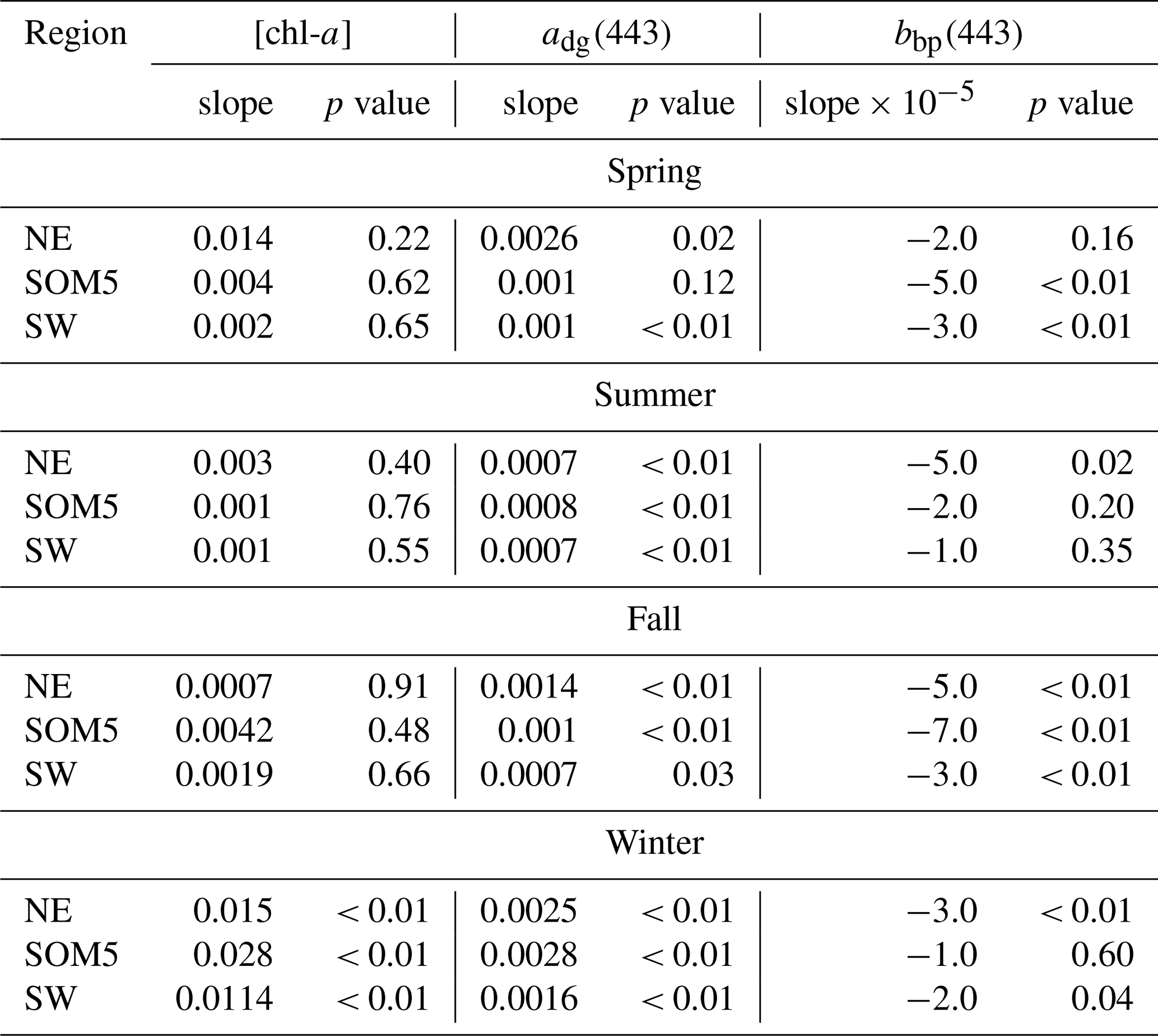
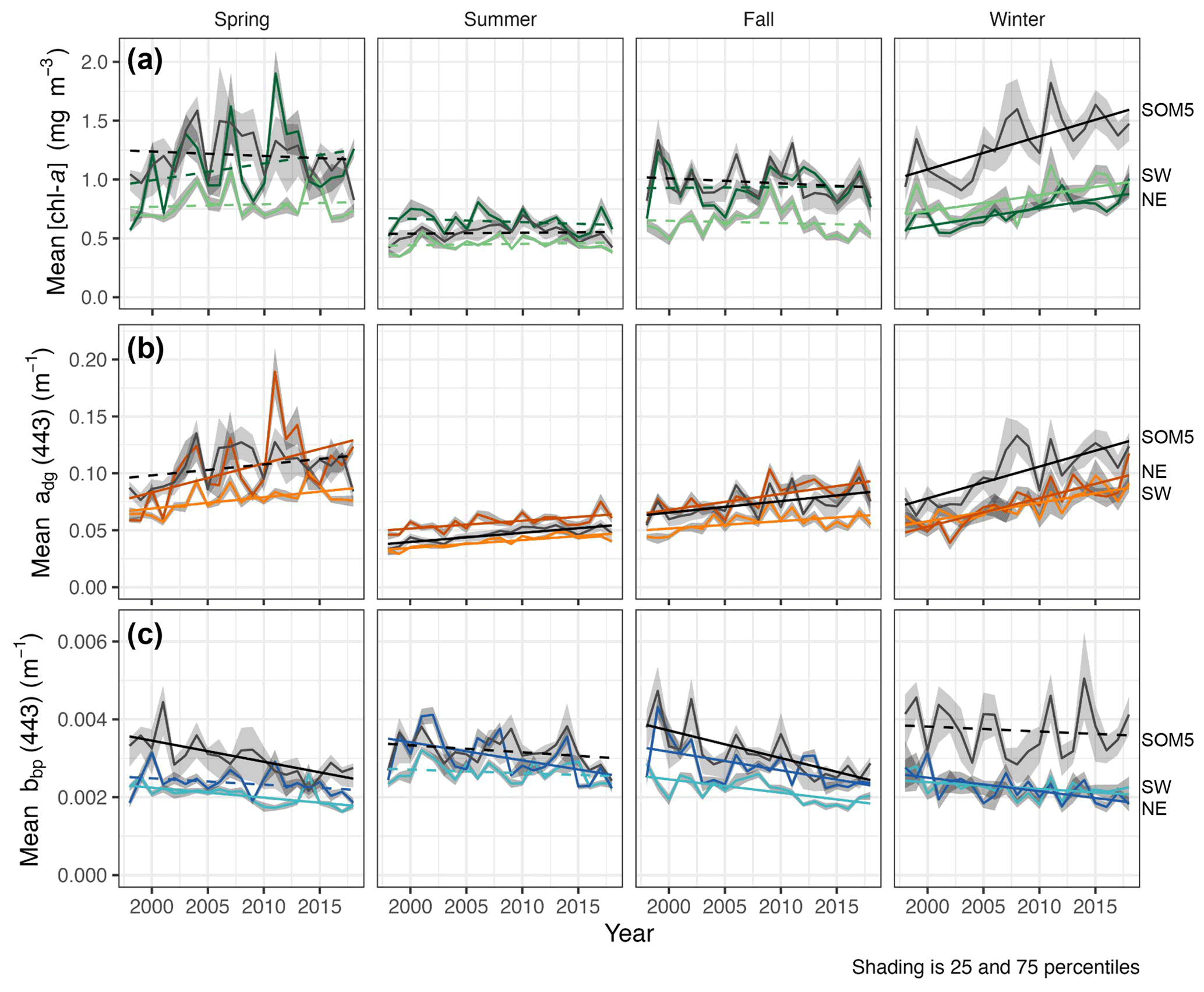
Figure 4Seasonal mean [chl-a] (a), adg(443) (b) and bbp(443) (c) for the SOM5 region (i.e., plume southwest of SI in SOM node no. 5 where [chl-a] is greater than 1 mg m−3) and control boxes (NE and SW). Statistically significant trends (p value < 0.05) are shown as solid lines, while non-significant trends are dashed. Line regions are labelled on the right.
The seasonal [chl-a] trends were significant in winter for all three regions of interest (ROIs; Fig. 4a and Table 1), while no trends in [chl-a] were observed in these ROIs for the other seasons. It is noteworthy that the rate of increase in [chl-a] over the period of observation for the plume near SI (i.e., SOM5) was twice that of the control boxes. The adg(443) linear trend was also positive and significant in all three ROIs in winter (Fig. 4b). The highest increase was observed in winter around SI (slope of 0.0028 ) as for the [chl-a] trend; the second highest positive linear trend was also observed in winter in the NE box (0.0025 ). For the other seasons, the increase, when significant, was much smaller. In summer, the slope was significant and around 0.0007 for all three ROIs, while for spring and fall the results were more variable, with only the SW region showing a significant positive trend in summer and the SOM5 and NE regions showing a significant positive trend in fall. The backscattering coefficient showed significant declines in all seasons and ROIs except for the NE in spring, SI and SW in summer, and SI in winter (Fig. 4c). These findings are consistent with changes in hydrodynamic forcing observed on the Scotian Shelf and, in particular, an increase in stratification (Hebert et al., 2021), which could explain the decrease in particle resuspension and hence the decrease in bbp(443).

Figure 5Mean [chl-a] in winter for the four periods of interest. The white solid line represent the 1 mg m−3 contour.
When averaging the winter [chl-a] over a 5-year period (Fig. 5), the increase in [chl-a] was even more striking, as it revealed both the increase in magnitude within the plume and the increase in the plume surface area. Our study shows that not only does SI have a local effect on the surrounding ecosystem as enhanced [chl-a] is observed in the leeward region of the island, but also that the phytoplankton biomass has increased in winter over the last two decades at a rate not matched by the other regions (i.e., control boxes).
The SOM and trend analysis responded to the second question raised in the introduction and provided information on the dynamics of the chl-a plume southwest of SI, and notably they showed the large extent of the plume in winter and an increase in [chl-a] over the last 21 years that was particular to the SOM5 region.
3.2.1 Simultaneous increase in seal abundance and phytoplankton biomass, a coincidence?
The position of SI near the continental shelf may explain some of the elevated [chl-a] (hypothesis 3), due to the warm slope waters advecting on the Scotian Shelf from the continental slope (Petrie and Drinkwater, 1993) bringing nutrients from horizontal and vertical mixing (Zhai et al., 2011); however, if that was the case, this phenomenon would occur along the entire slope and also in the SW box, which was not evidenced. In addition, repeated measurements of nutrients over the entire Scotian Shelf over the last 20 years have revealed a continuous decrease in nitrate concentration since about 2012, in agreement with an increase in stratification (Casault et al., 2020). Therefore, physical forcing and advection of nutrients alone cannot explain the increase in [chl-a] in the SOM5 region.
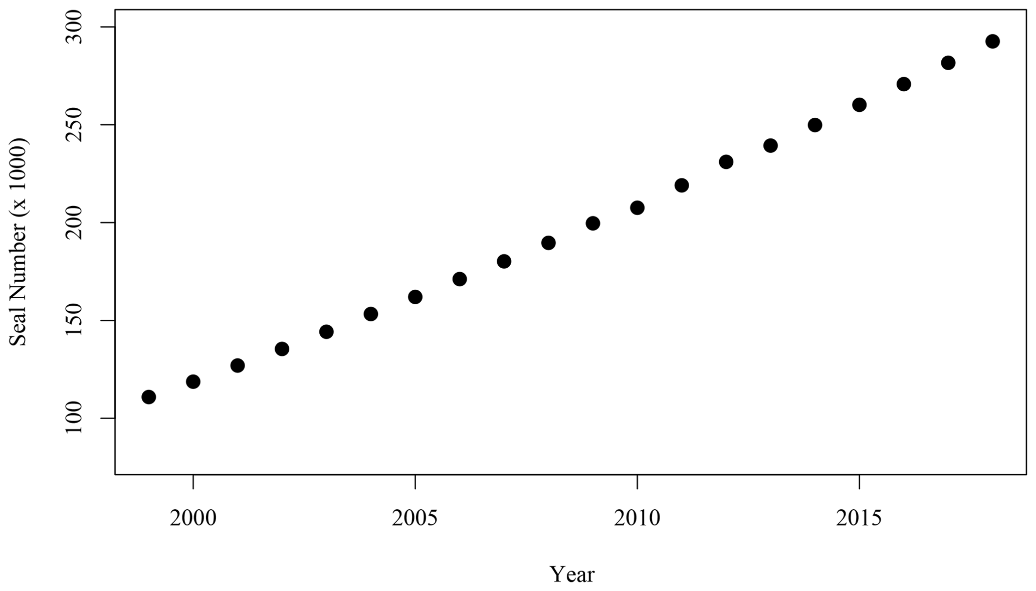
Figure 6Number of adult (age 1+) grey seals associated with the SI breeding colony (Rossi et al., 2021).
While the hypotheses stated above did not provide a satisfactory explanation of the spatio-temporal pattern occurring leeward of SI, an interesting parallel to the satellite observations over the same time period was the large increase in the population of grey seal (Halichoerus grypus), particularly during the breeding season in the winter months (December through February, Fig. 6). Fecal matter from marine mammals including pinnipeds and whales liberates nitrogenous compounds including (Roman and McCarthy, 2010) to the environment. Fertilisation of the ocean by marine mammals and birds has been demonstrated in several regions of the world (e.g., Roman and McCarthy, 2010; Laver et al., 2012; Mccauley et al., 2012; Wing et al., 2014). In the Gulf of Maine, adjacent to the Scotian Shelf, Roman and McCarthy (2010) estimated that whales and seals provide up to 2.3 × 10⁴ t N yr−1 to the surface waters. A parallel was therefore made between the contribution of the growing population of grey seals on SI and the increase in phytoplankton biomass around SI, particularly considering that has been shown to be used preferentially to nitrate by phytoplankton on the Scotian Shelf (Cochlan, 1986).

Figure 7Satellite-derived 8 d mean (solid circles) and smoothing (solid lines) of chl-a standing stocks in the SOM5 region for the periods 1999–2003 (red) and 2014–2018 (black). The green solid line corresponds to the difference between the two periods. The grey dashed line corresponds to the [chl-a] phenology in the NE box, assumed free of N fertilisation by seals.
3.2.2 Seal abundance on SI and chl-a standing stocks in SOM5
The difference in satellite-derived chl-a standing stocks between the period 1993–2003 and the period 2014–2018 was most important from winter to early spring (Fig. 7), with the most recent period (P4) higher than the reference period (P1). The maximum difference is reached in early March, with an excess of 134 t of chl-a, following a steady increase that started in early December. From late spring to fall, the difference between the two periods ranged between −50 and +10 t of chl-a. The results observed in the SOM5 region were in agreement with the decadal trend analysis that did not show any trends in [chl-a] in spring, summer and fall in the SOM5 region (Table 1 and Fig. 4), while winter showed the highest rate of increase (0.028 ). Regardless, the presence of seals on the island has been increasing during spring, summer and fall. The faster rate of increase in winter could suggest that there has been a change in the distribution of seals as the population has grown, with a smaller proportion of seals using SI as a haul-out location outside of the breeding season. The spring bloom during P4 is somewhat masked by high [chl-a] that started to occur in early December (Fig. 7).
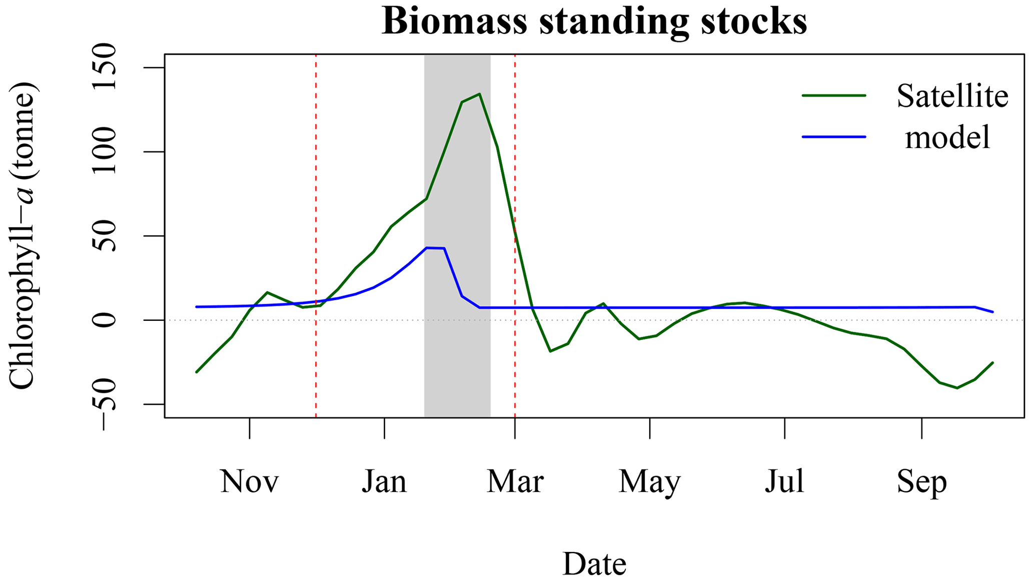
Figure 8Increase in chl-a standing stocks between P1 and P4 (green solid line) and modelled chl-a standing stocks due to seal N release in the environment (blue solid line). The vertical red dashed line corresponds to the arrival and departure of seal on SI (i.e., breeding season), and the light grey rectangle corresponds to the 8 d climatology of air temperature that is below zero.
Based on telemetry data (Breed et al., 2011), grey seal abundance year long on SI is about 16 % of the total adult population, or about 40 000 individuals are hauled out on SI outside of the breeding season. Seals defer digestion and therefore defecation during rest time, suggesting that they may, indeed, relieve themselves on SI or its surroundings rather than during foraging in the ocean (Sparling et al., 2007). The daily pattern of N release, which was further converted into chl-a standing stocks following Roman and McCarthy (2010) and Matear (1995), is a multiplicative term based on an average rate per individual. As the telemetry data show that larger male grey seals spend more time using SI as a haul-out location in winter, our estimate, based on the average duration of time hauled out, is a conservative estimate of N flux per individual. There is a good temporal agreement between the standing stock of chl-a derived by satellite and modelled with a Pearson correlation coefficient of 0.54 (Fig. 8), which increased to 0.86 when using a 24 d lag (i.e., corresponding to three 8 d periods), with the chl-a standing sock reaching its peak later than the peak in N release. We found that for the period P4, annual N released by seals could support about 580 t of chl-a (Fig. A1), while the biomass standing stocks sustained by seals during the breeding period equal 297 t when including the 24 d lag. About 50 % of the potential chl-a standing stocks due to seal fertilisation would occur during the breeding season. We have also estimated the winter chl-a standing stocks using both satellite observations and the model of hauled out seals in four 5-year blocks. The seal-supported chl-a annual standing stock (i.e.158 t) accounts for about 21 % of the increase between P4 and P1 derived by satellite observations (i.e., 761 t, Fig. 8). These annual estimates did not account for breeding behaviour or sexual dimorphism, which could have an impact on the estimates of N release at the breeding colony, where females fast during lactation and much larger males spend higher proportion of time hauled out. Similarly, for the satellite-observed [chl-a], we used conversion factors from the literature to derive the daily nutrient release and chl-a standing stocks from the seal population model. We used a conversion factor of N to chl-a of 1.59 mg chl a (mmol N)−1, in agreement with Yentsch and Vaccaro (1958) and Matear (1995); however, William et al. (2010) found a conversion factor that varies from 1.1 mg chl a (mmol N)−1 on an intra-daily scale to 1.4 mg chl a (mmol N)−1 at a weekly scale during the spring bloom; using this value would further reduce the chl-a standing stocks that could be sustained by seals. The satellite observations were mainly constrained by the assumption of an homogeneous profile of [chl-a] from 0 to 50 m and the delineation of the plume. Here we decided on a 1 mg m−3 threshold to delineate the plume in the SOM5 region, which was consistent with the description of a phytoplankton bloom on the Scotian Shelf. Using a smaller threshold would have increased the surface area of the plume and increased the chl-a standing stocks estimates; however, the general patterns and notably the temporal variation would remain the same. To test the mechanisms that can explain the increase in [chl-a], in situ sampling of standing stocks and water chemistry surrounding SI is necessary.
The lag observed between the peaks in seal abundance and phytoplankton biomass in the plume can be explained by several factors, including (1) the transport of seal feces to the ocean, which will certainly take a few days and depends on atmospheric forcing, soil permeability, sea state and tide, with storm surges inundating the beach and releasing organic material; (2) the negative air temperatures that occur between the end of January and February (Fig. B2), which would reduce and delay the diffusion of N from SI to the adjacent waters, when the soil is frozen and precipitation occurs as snow; and (3) day length, which increases by about an hour from about 9 h and 45 min to 11 h and 5 min between early January and the end of February, which will increase primary production over this period as N is not the limiting factor. Undoubtedly, other environmental factors contribute to the production of biomass in the area of interest (e.g., atmospheric forcing, timing and strength of stratification, light availability) but are not taken into account in our conceptual model.
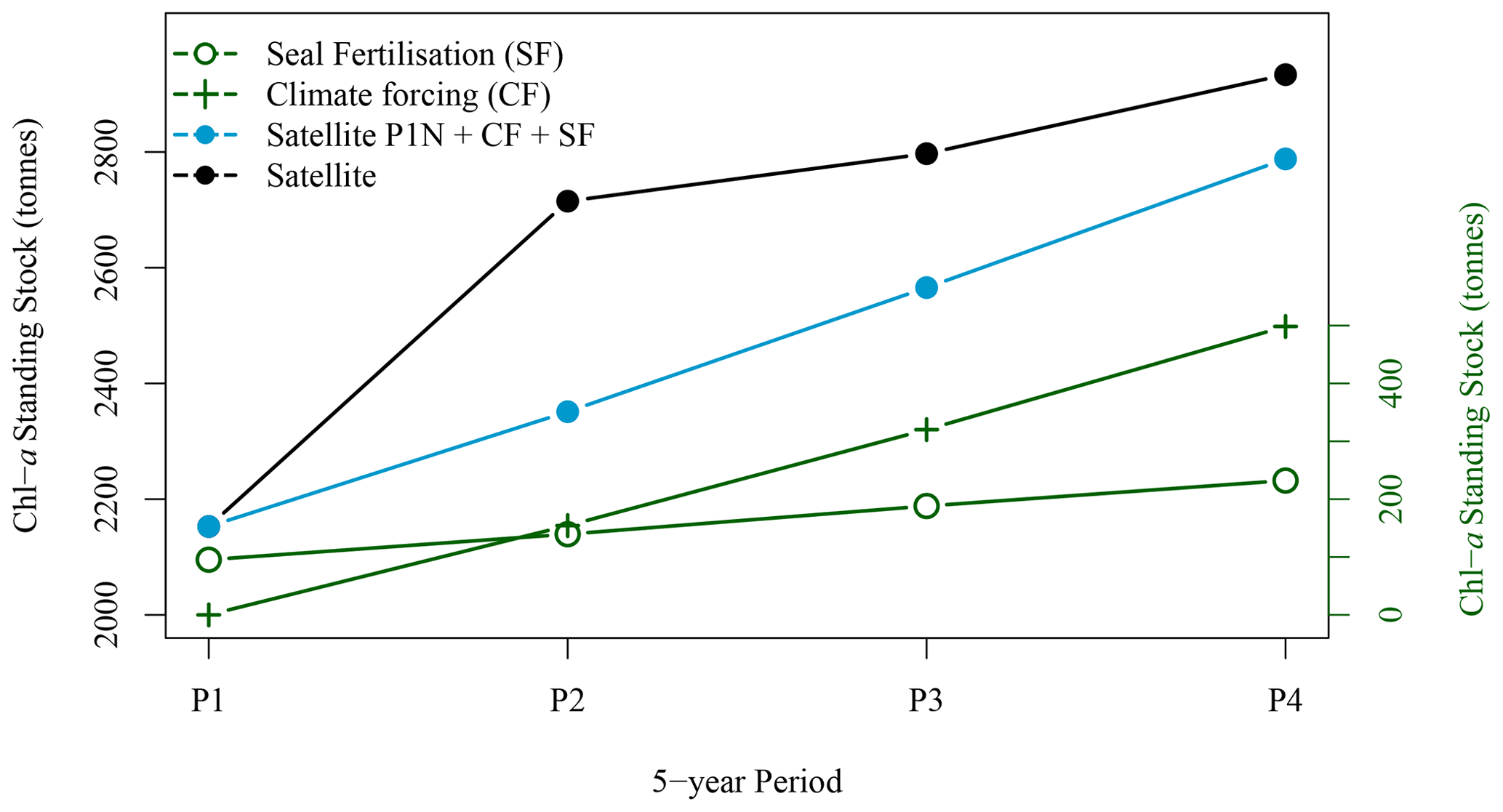
Figure 9Five-year winter average standing stock of chl-a derived from satellite observations (solid black circle), from satellite observation for P1 extrapolated with climate forcing and seal N fertilisation (blue solid circles), from climate forcing (green crosses) and from seal N fertilisation (green open circles) for the four periods of interest (black solid circles).
3.2.3 Synchronised decadal increase in seal population, extent and concentration of the chl-a plume around SI
The winter increase in chl-a standing stocks in the leeward region of SI (SOM5) was consistent with the increase in seal population on SI over the last 21 years. From the late 1990s to the late 2010s, pup production at the breeding colony has increased at a rate of about 5–7 % yr−1 (Fig. 6 den Heyer et al., 2020). We demonstrated that the average [chl-a] increased within the plume southward of SI at a faster rate than the surrounding control boxes in winter. In terms of the 5-year average standing stocks of chl-a over the four periods of interest, P1 to P4 (Fig. 9), a quasi-linear increase in chl-a standing stocks was observed, except for the period P2, which slightly departs from linearity. The high values for P2 were due to a sudden increase in chl-a standing stocks during a large bloom occurring in early December, a phenomenon that may be explained by natural variation in phytoplankton biomass, and notably a short growth period that can occur on the Scotian Shelf when conditions are favourable. The increase in chl-a standing stocks due to climate forcing was computed by taking the value during P1 and subtracting the chl-a standing stocks due to N fertilisation by seals and then applying a mean 5-year rate of increase of 0.075 taken from the annual rate of increase at the NE box (i.e., 0.015 ). This provided chl-a standing stocks of 2947, 3619, 3923 and 3709 t for P1N, P2N, P3N and P4N, respectively, which corresponded to an increase in chl-a standing stocks of 154, 317 and 489 t between each 5-year time period (Fig. 9). During the same periods, the contribution by seal fertilisation to chl-a standing stocks was 139, 188, 241 and 297 for P1, P2, P3 and P4, respectively. The sum of the chl-a standing stocks due to the natural increase and seal fertilisation matches the total chl-a standing stocks observed using satellite ocean colour for the period P1 and P4, while a large discrepancy was observed for the period P2 and P3 (Fig. 9). The main difference occurred during the period P2 with a difference of 215 t between both estimations. For the period P4, the combined climate forcing and seal fertilisation provided a very similar estimate than the one observed by satellite. The linear increase due to climate forcing might be too simplistic as large interannual variations exist and Liu et al. (2018) showed that the increase in [chl-a] on the Scotian Shelf slowed down after 2012, but the consistency between both estimates remains remarkable. The contribution by seal N fertilisation to the total chl-a standing stocks in SOM5 has increased from 4.7 % to 8 % between P1 to P4 and the contribution by climate forcing increased from 4.2 % to 13.1 % between P2 and P4. As for the seasonal cycle, the satellite estimates provided here depended on the delineation of the plume southward of SI; the value selected here (i.e., 1 mg m−3) happened to provide a good agreement between the model and the satellite observations.
Sable Island, a large sandbar located at the edge of the continental shelf off eastern Canada, sees enhanced [chl-a] and yellow substance concentration in its vicinity and in particular leeward of the island as revealed by satellite ocean colour. This finding is in agreement with the island mass effect theory that has been demonstrated in other parts of the world. The increase and phenology of phytoplankton biomass around SI was demonstrated by comparison with two control boxes located to the northeast (NE) and southwest (SW) of SI, away from possible terrigenous inputs. We found that [chl-a] around SI showed a different annual cycle than the control boxes with higher values in late fall through winter. This was also the case for the absorption coefficient of DOM and the backscattering coefficient. Using an objective classification method (i.e., self organising maps), we were able to describe the spatio-temporal variation of [chl-a] on the Scotian Shelf in general and around SI in particular. A distinct pattern of high [chl-a] around SI, the region referred to as SOM5, was revealed by this analysis and occurred from late fall through winter; comparison with the [chl-a] phenology in the control boxes showed that this pattern was different than the fall bloom and singular to SI. In addition, analysis of seasonal trends in mean [chl-a] showed only a significant increase in the three regions of interest in winter but with a trend twice as high for SI than for the SW and NE boxes, i.e., 0.028 mg yr−1. The absorption coefficient, adg(443), showed a positive trends in all regions in winter and summer but some regional differences for spring and fall. For bbp(443), one observed a significant decreasing trend in all regions in fall only. The results highlighted the possible link between variations in [chl-a] and adg(443), while variations in bbp(443) seemed to be the results of hydrodynamic forcing.
The location of SI (away from continental inputs) and the analysis of adg(443) and bbp(443) seasonal cycles and decadal trends did not help explain the processes that led to the increase in [chl-a] around SI, as no trends in particulate backscattering and DOM absorption were markedly different from the surrounding environment. Notably, the seal population that breeds on SI increased from about 100 000 to more than 300 000 individuals from 1999 to 2018. We developed a simple model that describes the seal occurrence on SI, in particular during the reproductive season (i.e., early December to February), and converted the daily theoretical N release due to seal excretion to chl-a standing stocks. Comparison of the model results with satellite-derived chl-a standing stocks shows a good agreement, not only in terms of the seasonal cycle, but also to the decadal trends. Both the mean [chl-a] increased within the plume located leeward of the island and the plume surface area increased by a factor of 5 over the period of observation, which was also a period of rapid growth for the grey seal population.
The seal population on SI exceeded 300 000 individuals in recent years, and the associated N release in the surrounding waters can support chl-a standing stocks of 297 t in winter, in agreement with standing stocks observed in the SI chl-a plume in recent years. While we acknowledge the lack of in situ measurements in the surrounding waters of SI, the good agreement between our model results and satellite observations support the role that grey seals can play at haul-out sites and breeding colonies. Our results are consistent with Roman and McCarthy (2010), who found that marine mammals (both seals and cetaceans) could support 2.3 × 10⁴ t of nitrogen in the Gulf of Maine. The high concentration of seals on a small island located at the edge of the continental shelf for a short period of time represents ideal conditions to witness their impact on the marine ecosystem; however, this impact is certainly diminished when they leave the breeding colony to forage over very large areas (i.e., the Scotian Shelf, Gulf of St. Lawrence, Gulf of Maine and Grand Banks). Here we see evidence for the transfer of nutrients from benthic fish communities (i.e., seal prey) to surface waters near SI, with implications for marine conservation and fisheries.
The annual seal population distribution on SI was estimated using information on pup production from Rossi et al. (2021) and den Heyer et al. (2020). The mathematical formulation is described in Sect. 2.5.1, Eq. (1). The model was also applied to the 5-year average seal abundance on SI for the periods P1 to P4 (Table A1) and used to generate the chl-a standing stocks in Fig. 9. Note that fluctuations around the mean seal abundance outside the breeding season is expected but not accounted for in the model.
Table A1Five-year average of seal haul-out on SI all year long and during the breeding season used in the seal population dynamic model.

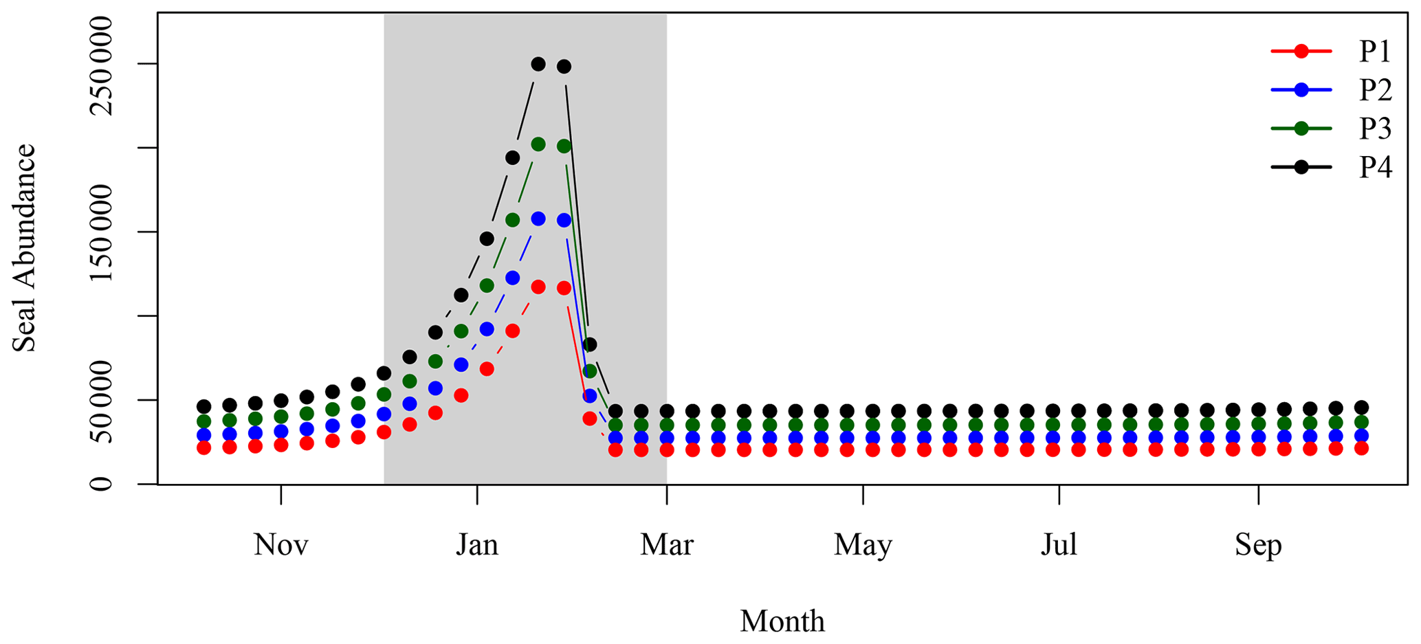
Figure A1Annual cycle of seal hauls on SI for the four period of interest. The grey shaded area corresponds to the breeding season.
Daily data at the SI weather station were downloaded from the ECCC website (https://climate.weather.gc.ca/historical_data/search_historic_data_e.html, last access: 16 November 2021). Data from the station 8204700 (1998–2017) and 8204708 (2018) were used. The temperature and precipitation 8 d climatology was computed by averaging all data available in a given 8 d period for all years. The standard deviation is indicated with the mean in both Figs. B1 and B2.
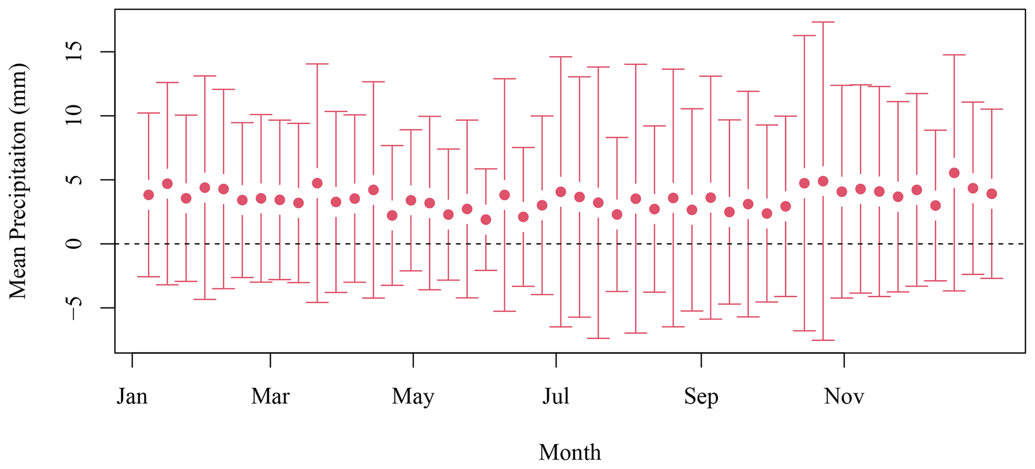
Figure B1The 8 d composite climatology of precipitation SI meteorological stations (solid circles). The vertical bars indicate 1 standard deviation.
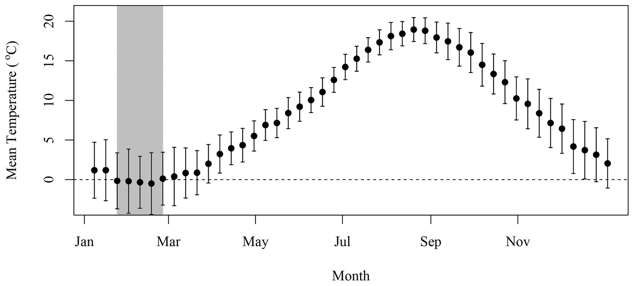
Figure B2The 8 d composite climatology of air temperature over SI (solid circles). Vertical bar indicates 1 standard deviation.

Figure C1Monthly mean surface velocity of on the Scotian Shelf from the OSCAR dataset. Numbers in the grey banner correspond to the month of the year; e.g., 1 corresponds to January while 12 corresponds to December.
All data used in the study are in the public domain. Ocean Colour satellite datasets were obtained from the Ocean Colour Climate Change Initiative: https://oceancolour.org/browser/ (ESA and PML, 2021). The dataset on oceanic current was downloaded from https://coastwatch.pfeg.noaa.gov/erddap (NOAA, 2021), and the meteorological dataset was downloaded from Environment and Climate Change Canada: https://climate-change.canada.ca/climate-data/#/daily-climate-data (Government of Canada, 2021). The SOM maps are available upon request. All computations were carried out using the R package, and the code is available upon request.
ED and CEdH initially discussed the idea of seal fertilisation around SI. ED designed the study. AH carried out all computations and statistical analysis related to satellite data. ED and CEdH developed the seal distribution model and chl-a standing stock budget. AH and ED contributed equally to the drafting of the manuscript. AH, CEdH and ED all contributed to the editing of the manuscript.
The authors declare that they have no conflict of interest.
Publisher's note: Copernicus Publications remains neutral with regard to jurisdictional claims in published maps and institutional affiliations.
We thank the NASA Goddard Space Flight Center, Ocean Ecology Laboratory, Ocean Biology Processing Group, for making the Aqua-MODIS data used in this study freely available.
The study was supported by Fisheries and Oceans Canada as well as the Canadian Space Agency Climate Change Impact and Ecosystem Resilience programme.
This paper was edited by Julia Uitz and reviewed by two anonymous referees.
Ainsworth, E. J.: Visualization of Ocean Colour and Temperature from multi-spectral imagery captured by the Japanese ADEOS satellite, J. Visual., 2, 195–204, https://doi.org/10.1007/BF03181523, 1999. a
Boden, B. P.: Observations of the island mass effect in the Prince Edward archipelago, Polar Biol., 61–68, 260–265, https://doi.org/10.1007/BF00441765, 1988. a
Boss, E., Stramski, D., Bergmann, T., Pegau, W., and Marlon, L.: Why Should We Measure the Optical Backscattering Coefficient?, Oceanography, 17, 44–49, https://doi.org/10.5670/oceanog.2004.46, 2004. a
Bowen, W. D., McMillan, J. I., and Wade, B.: Reduced population growth of gray seals at Sable Island: evidence from pup production and age of primiparity, Mar Mammal Sci., 23, 48–64, https://doi.org/10.1111/j.1748-7692.2006.00085.x, 2007. a, b
Breed, G. A., Bowen, D. W., McMillan, J., and Leonard, M. L.: Sex segregation of seasonal foraging habitats in a non-migratory marine mammal, P. R. Soc. B, 273, 2319–26, https://doi.org/10.1098/rspb.2006.3581, 2006. a
Breed, G. A., Bowen, D. W., and Leonard, M. L.: Development of foraging strategies with age in a long-lived marine predator, Mar. Ecol. Prog. Ser., 431, 267–279, https://doi.org/10.3354/meps09134, 2011. a
Breed, G. A., Bowen, D. W., and Leonard, M. L.: Behavioral signature of intraspecific competition and density dependence in colony-breeding marine predators, Ecol. Evol., 3, 3838–3854, https://doi.org/10.1002/ece3.754, 2013. a, b, c
Brickman, D. and Drozdowski, A.: Atlas of Model Currents and Variability in Maritime Canadian Waters, Tech. Rep. 277: vii + 64 pp., Can. Tech. Rep. Hydrogr. Ocean Sci., 2012. a, b
Bukata, R., Jerome, J., Kondratyev, K., and Pozdnyakov, D.: Optical properties and remote sensing of inland and coastal waters, CRC Press, Boca Raton, Fl, 1995. a
Casault, B., Johnson, C., Devred, E., Head, E. J. H., Cogswell, A., and Spry, J.: Optical, Chemical, and Biological Oceanographic Conditions on the Scotian Shelf and in the Eastern Gulf of Maine during 2019, in: Can. Sci. Advis. Sec. Res. Doc., p. 64, DFO, 2020. a, b, c
Cochlan, W. P.: Seasonal study of uptake and regeneration of nitrogen on the Scotian Shelf, Cont. Shelf Res., 5, 555–577, https://doi.org/10.1016/0278-4343(86)90076-2, 1986. a
Dandonneau, Y. and Charpy, L.: An empirical approach to the island mass effect in the south tropical Pacific based on sea surface chlorophyll concentrations, Deep-Sea Res. Pt. A, 32, 707–721, https://doi.org/10.1016/0198-0149(85)90074-3, 1985. a, b
den Heyer, N., Bowen, W., Dale, J., Gosselin, J. F., Hammill, M., Johnston, D., Lang, S., Murray, K., Stenson, G., and Wood, S.: Contrasting trends in gray seal (Halichoerus grypus) pup production throughout the increasing northwest Atlantic metapopulation, Mar Mammal Sci., 37, 611–630, https://doi.org/10.1111/mms.12773, 2020. a, b, c, d, e
Denman, K. L. and Platt, T.: The variance spectrum of phytoplankton in a turbulent ocean, J. Mar. Res., 34, 593–6016, 1976. a
Doty, M. S. and Oguri, M.: The Island Mass Effect, ICES J. Mar. Sci., 22, 33–37, https://doi.org/10.1093/icesjms/22.1.33, 1956. a
ESA and PML: Ocean Coulour Climate Change initiative, available at: https://oceancolour.org/browser/, last access: 17 November 2021. a
Gilmartin, M. and Revelante, N.: The “island mass” effect on the phytoplankton and primary production of the Hawaiian Islands, J. Exp. Mar. Biol. Ecol., 16, 181–204, https://doi.org/10.1016/0022-0981(74)90019-7, 1974. a
Gove, J. M., McManus, M. A., Neuheimer, A. B., Poloniva, J. J., Draven, J. C., Smith, C. R., Merrifield, M. A., Friedlander, A. M., Ehses, J. S., Young, C. W., Dillon, A. K., and Williams, G. J.: Near-island biological hotspots in barren ocean basins, Nat. Commun., 7, 154–157, https://doi.org/10.1038/ncomms10581, 2016. a, b, c
Government of Canada: Daily climate data, available at: https://climate-change.canada.ca/climate-data/#/daily-climate-data, last access: 18 November 2021. a
Hammill, M. O., Stenson, G. B., Swain, D. P., and Benoît, H. P.: Feeding by grey seals on endangered stocks of Atlantic cod and white hake, ICES J. Mar. Sci., 71, 1332–1341, https://doi.org/10.1093/icesjms/fsu123, 2014. a
Hardman-Mountford, N., Richardson, A., Boyer, D., Kreiner, A., and Boyer, H.: Relating sardine recruitment in the Northern Benguela to satellite-derived sea surface height using a neural network pattern recognition approach, Prog. Oceanogr., 59, 241–255, https://doi.org/10.1016/j.pocean.2003.07.005, 2003. a
Hebert, D., Layton, C., Brickman, D., and Galbraith, P.: Physical Oceanographic Conditions on the Scotian Shelf and in the Gulf of Maine during 2019, in: Can. Sci. Advis. Sec. Res. Doc., 2021/040, pp. iv + 58, DFO, 2021. a
Heywood, K., Barton, E. D., and Simpson, J.: The effects of flow disturbance by an oceanic island, J. Mar. Res., 48, 55–73, https://doi.org/10.1357/002224090784984623, 1990. a
Jackson, T., Chuprin, A., Sathyendranath, S., Grant, M., Zühlke, M., Dingle, J., Storm, T., and ad N. Fomferra, M. B.: Product User Guide, Tech. rep., European Space Agency, available at: https://docs.pml.space/share/s/okB2fOuPT7Cj2r4C5sppDg (last access: 16 November 2021), 2020. a
James, A. K., Washburne, L., Gotschalks, C., Maritorena, S., Alldredge, A., Nelson, C. E., Hench, J. L., Leichter, J. J., Wyat, A. S. J., and Carlson, C. A.: An Island Mass Effect Resolved Near Mo'orea, French Polynesia, Frontiers in Marine Science, 7, 16, https://doi.org/10.3389/fmars.2020.00016, 2020. a, b
Kanwisher, J. and Ridgway, S.: The Physiological Ecology of Whales and Porpoises, Sci. Am., 248, 110–120, https://doi.org/10.1038/scientificamerican0683-110, 1983. a
Kennedy, G. W., Drage, J., and Hennigar, T. W.: Groundwater Resources of Sable Island, Tech. rep., Open File Report ME 2014-001, Nova Scotia Department of Natural Resources, Mineral Resources Branch, Government of Nova Scotia, available at: https://novascotia.ca/natr/meb/data/pubs/14ofr01/14ofr01.pdf (last access: 16 November 2021), 2014. a
King, M., Fenton, D., Aker, J., and Serdynska, A.: Offshore Ecologically and Biologically Significant Areas in the Scotian Shelf Bioregion, Tech. Rep. 2016/007. vii + 92 p., DFO Can. Sci. Advis. Sec. Res. Doc., 2016. a, b
Laver, T., Roudnew, B., Seymou, J., Mitchell, J., and Jeffries, T.: High nutrient transport and cycling potential revealed in the microbial metagenome of Australian sea lion (Neophoca cinerea) faeces, PloS one, 7, e36 478, https://doi.org/10.1371/journal.pone.0036478, 2012. a, b
Lee, Z. P., Du, K., Arnone, R., Liew, S. C., and Penta, P.: Penetration of solar radiation in the upper ocean – A numerical model for oceanic and coastal waters, J. Geophys. Res., 110, C09019, https://doi.org/10.1029/2004JC002780, 2005. a
Liu, X., Devred, E., and Johnson, C.: Remote Sensing of Phytoplankton Size Class in Northwest Atlantic from 1998 to 2016: Bio-Optical Algorithms Comparison and Application, Remote. Sens.-Basel, 10, 1028, https://doi.org/10.3390/rs10071028, 2018. a
Loder, J., Han, G., Hannah, C. G., Greenberg, D. A., and Smith, P. C.: Hydrography and baroclinic circulation in the Scotian Shelf region: winter versus summer, Can. J. Fish. Aquat. Sci., 54, 40–56, https://doi.org/10.1139/cjfas-54-S1-40, 1997. a, b
Lunne, T., Robertson, P. K., and Powell, J.: Cone-penetration testing in geotechnical practice, Soil Mech. Found. Eng., 46, 237, https://doi.org/10.1007/s11204-010-9072-x, 2009. a
Martinez, E. and Maamaatuaiahutapu, K.: Island mass effect in the Marquesas Islands: Time variation, Geophys. Res. Lett., 31, L18307, https://doi.org/10.1029/2004GL020682, 2004. a
Martinez, E., Raapotoi, H., Maes, C., and Maamaatuaiahutapu, K.: Influence of Tropical Instability Waves on Phytoplankton Biomass near the Marquesas Islands, Remote Sens.-Bael, 10, 640, https://doi.org/10.3390/rs10040640, 2018. a
Matear, R.: Parameter optimization and analysis of ecosystem models using simulated annealing: A case study at Station P, J. Mar. Res., 53, 571–607, https://doi.org/10.1357/0022240953213098, 1995. a, b, c
Mccauley, D., Desalle, P., Young, H., Dunbar, R., Dirzo, R., Mills, M., and Micheli, F.: From wing to wing: The persistence of long ecological interaction chains in less-disturbed ecosystems, Sci. Rep.-UK, 2, 409, https://doi.org/10.1038/srep00409, 2012. a, b
McLoughlin, P. D., Lysak, K., Debeffe, L., Perry, T., and Hobson, K. A.: Density-dependent resource selection by a terrestrial herbivore in response to sea-to-land nutrient transfer by seals, Ecology, 97, 1929–1937, https://doi.org/10.1002/ecy.1451, 2016. a
Messié, M., Petrenko, A., Doglioli, A., Aldebert, C., Martine, E., Koenig, G., and T. Moutin, S. B.: The Delayed Island Mass Effect: How Islands can Remotely Trigger Blooms in the Oligotrophic Ocean, Geophys. Res. Lett., 47, e2019GL085282, https://doi.org/10.1029/2019GL085282, 2020. a, b
Moore, T., Dowell, M., and Franz, B.: Detection of coccolithophore blooms in ocean color satellite imagery: A generalized approach for use with multiple sensors, Remote Sens. Environ., 117, 249–263, https://doi.org/10.1016/j.rse.2011.10.001, 2012. a
Morel, A. and Prieur, L.: Analysis of variation in ocean color, Limnol. Oceanogr., 22, 709–722, 1977. a
Neuenhoff, R. D., Swain, D. P., Cox, S. P., McAllister, M. K., Trites, A. W., Walters, C. J., and Hammill, M. O.: Continued decline of a collapsed population of Atlantic cod (Gadus morhua) due to predation-driven Allee effects, Can. J. Fish. Aquat. Sci., 76, 168–184, https://doi.org/10.1139/cjfas-2017-0190, 2019. a
NOAA: ERDDAP, available at: https://coastwatch.pfeg.noaa.gov/erddap, last access: 17 November 2021. a
O'Boyle, R. and Sinclair, M.: Seal–cod interactions on the Eastern Scotian Shelf: Reconsideration of modelling assumptions, Fish. Res., 115–116, 1–13, https://doi.org/10.1016/j.fishres.2011.10.006, 2012. a, b, c
Petrie, B. and Drinkwater, K.: Temperature and salinity variability on the Scotian Shelf and in the Gulf of Maine 1945–1990, J. Geophys. Res., 982, 20 079–20 090, https://doi.org/10.1029/93JC02191, 1993. a
R Core Team: R: A Language and Environment for Statistical Computing, R Foundation for Statistical Computing, Vienna, Austria, available at: https://www.R-project.org/ (last access: 16 November 2021), 2020. a
Richardson, A. J., Risien, C., and Shillington, F. A.: Using self-organizing maps to identify patterns in satellite imagery, Prog. Oceanogr., 59, 223–239, https://doi.org/10.1016/j.pocean.2003.07.006, 2003. a, b, c
Roman, J. and McCarthy, J. J.: The Whale Pump: Marine Mammals Enhance Primary Productivity in a Coastal Basin, PLoS ONE, 5, e13255, https://doi.org/10.1371/journal.pone.0013255, 2010. a, b, c, d, e, f, g
Rossi, S., Cox, S., den Heyer, M. H. C. E., Mosnier, D. S. A., and Benoît, H.: Forecasting the response of a recovered pinniped population to sustainable harvest strategies that reduce their impact as predators, ICES J. Mar. Sci., 78, 1804–1814, https://doi.org/10.1093/icesjms/fsab088, 2021. a, b, c, d
Sathyendranath, S., Brewin, B., Brockmann, C., Brotas, V., Calton, B., Chuprin, A., Cipollini, P., Cout, A., Dingle, J., R. Doerffer, R., Donlon, C., Dowell, M., Farman, A., Grant, M., Groom, S., Horseman, A., Jackson, T., Krasemann, H., Lavender, S., and Platt, T.: An Ocean-Colour Time Series for Use in Climate Studies: The Experience of the Ocean-Colour Climate Change Initiative (OC-CCI), Sensors, 19, 4285, https://doi.org/10.3390/s19194285, 2019. a
Sathyendranath, S., Jackson, T., Brockmann, C., Brota, V., Calton, B., A.Chuprin, Clements, O., Cipollin, P., Danne, O., Dingle, J., Donlon, C., Grant, M., Groom, S., Krasemann, H., Lavende, S., Mazeran, C., Mélin, F., T. S. Moore, T., Mülle, D., Regner, P., Steinmetz, F., Steele, C., Swinton, J., Valente, A., Zühlke, M., Feldman, G., Franz, B., Frouin, R., Werdell, J., and Platt, T.: ESA Ocean Colour Climate Change Initiative (Ocean_Colour_cci): Global chlorophyll-a data products gridded on a sinusoidal projection, Version 4.2, available at: https://catalogue.ceda.ac.uk/uuid/99348189bd33459cbd597a58c30d8d10 (last access: 16 November 2021), 2020. a
Siegel, D. A., Doney, S. C., and Yoder, J. A.: The North Atlantic spring phytoplankton bloom and Sverdrup's critical depth hypothesis, Science, 296, 730–733, 2002. a
Signorini, S. R., McClain, C. R., and Dandonneau, Y.: Mixing and phytoplankton bloom in the wake of the Marquesas Islands, Geophys. Res. Lett., 26, 3121–3124, https://doi.org/10.1029/1999GL010470, 1999. a, b
Slade, W. H. and Boss, E.: Spectral attenuation and backscattering as indicators of average particle size, Appl. Optics, 54, 7264–7277, https://doi.org/10.1364/AO.54.007264, 2015. a
Smith, P. C. and Schwing, F. B.: Mean circulation and variability on the eastern Canadian continental shelf, Cont. Shelf Res., 11, 977–1012, https://doi.org/10.1016/0278-4343(91)90088-N, 1991. a
Song, H., Ji, R., Stoc, C., and Wang, Z.: Phenology of phytoplankton blooms in the Nova Scotian Shelf-Gulf of Maine region: Remote sensing and modeling analysis, J. Plankton Res., 32, 1485–1499, https://doi.org/10.1093/plankt/fbq086, 2010. a
Sparling, C. E., Fedak, M. A., and Thompson, D.: Eat now, pay later? Evidence of deferred food-processing costs in diving seals, Biol. Letters, 3, 95–99, https://doi.org/10.1098/rsbl.2006.0566, 2007. a
Steinmetz, F., Deschamps, P., and Ramon, D.: Atmospheric correction in presence of sun glint: application to MERIS, Opt. Express, 19, 9783–9800, https://doi.org/10.1364/OE.19.009783, 2011. a
Theobald, M. R., Crittenden, P. D., Hunt, A. P., Tang, Y. S., Dragosits, U., and Sutton, M. A.: Ammonia emissions from a Cape fur seal colony, Cape Cross, Namibia, Geophys. Res. Lett., 33, L03812, https://doi.org/10.1029/2005GL024384, 2006. a
Trzcinski, M. K., Mohn, R., and Bowen, W. D.: Continued decline of an atlantic cod population: how important is gray seal predation?, Ecol. Appl., 16, 2276–2292, https://doi.org/10.1890/1051-0761(2006)016[2276:CDOAAC]2.0.CO;2, 2006. a
Ward-Paige, C. A. and Bundy, A.: Mapping Biodiversity on the Scotian Shelf and in the Bay of Fundy, Tech. Rep. 2016/006. v + 90 p., DFO Can. Sci. Advis. Sec. Res. Doc., 2016. a
Wehrens, R. and Buydens, L. M. C.: Self- and Super-organizing Maps in R: The kohonen Package, J. Stat. Softw., 21, 1–19, https://doi.org/10.18637/jss.v021.i05, 2007. a
Wehrens, R. and Kruisselbrink, J.: Flexible Self-Organizing Maps in kohonen 3.0, J. Stat. Softw., 87, 1–18, https://doi.org/10.18637/jss.v087.i07, 2018. a
William, K. W. L., Lewis, M. R., and Harrison, W. G.: Multiscalarity of the Nutrient–Chlorophyll Relationship in Coastal Phytoplankton, Estuar. Coast., 33, 440–447, 2010. a
Wing, S., Jack, L., Shatova, O., Leichter, J., Barr, D., R. Frew, R., and Gault-Ringold, M.: Seabirds and marine mammals redistribute bioavailable iron in the Southern Ocean, Mar. Ecol. Prog. Ser., 510, 1–13, https://doi.org/10.3354/meps10923, 2014. a, b
Yentsch, C. S. and Vaccaro, R. F.: Phytoplankton Nitrogen in the Oceans, Limnol. Oceanogr., 3, 443–448, https://doi.org/10.4319/lo.1958.3.4.0443, 1958. a, b
Zhai, L., Platt, T., Tang, C., Sathyendranath, S., and Hernández-Walls, R.: Phytoplankton phenology on the Scotian Shelf, ICES J. Mar. Sci., 68, 781–791, https://doi.org/10.1093/icesjms/fsq175, 2011. a, b, c, d
- Abstract
- Introduction
- Data and methods
- Results and discussion
- Conclusions
- Appendix A: Seal haul-out model
- Appendix B: Eight-day climatology of precipitation and temperature on SI
- Appendix C: Monthly surface currents from OSCAR dataset
- Data availability
- Author contributions
- Competing interests
- Disclaimer
- Acknowledgements
- Financial support
- Review statement
- References