the Creative Commons Attribution 4.0 License.
the Creative Commons Attribution 4.0 License.
 | 13 Dec 2021
Seasonal dispersal of fjord meltwaters as an important source of iron and manganese to coastal Antarctic phytoplankton
Lisa Hahn-Woernle
Robert M. Sherrell
Vincent J. Roccanova
Kaixuan Bu
David Burdige
Maria Vernet
Katherine A. Barbeau
Glacial meltwater from the western Antarctic Ice Sheet is hypothesized to be an important source of cryospheric iron, fertilizing the Southern Ocean, yet its trace-metal composition and factors that control its dispersal remain poorly constrained. Here we characterize meltwater iron sources in a heavily glaciated western Antarctic Peninsula (WAP) fjord. Using dissolved and particulate ratios of manganese to iron in meltwaters, porewaters, and seawater, we show that surface glacial melt and subglacial plumes contribute to the seasonal cycle of iron and manganese within a fjord still relatively unaffected by climate-change-induced glacial retreat. Organic ligands derived from the phytoplankton bloom and the glaciers bind dissolved iron and facilitate the solubilization of particulate iron downstream. Using a numerical model, we show that buoyant plumes generated by outflow from the subglacial hydrologic system, enriched in labile particulate trace metals derived from a chemically modified crustal source, can supply iron to the fjord euphotic zone through vertical mixing. We also show that prolonged katabatic wind events enhance export of meltwater out of the fjord. Thus, we identify an important atmosphere–ice–ocean coupling intimately tied to coastal iron biogeochemistry and primary productivity along the WAP.
- Article
(10840 KB) - Full-text XML
-
Supplement
(13611 KB) - BibTeX
- EndNote


Warm atmospheric temperatures are accelerating glacial retreat and increasing meltwater discharge, rapidly changing Earth's cryosphere (Mouginot et al., 2019; Rignot et al., 2013). Ranging from diffuse flows to waterfalls and streams, cryospheric meltwaters deliver dissolved and particulate material, altering coastal ocean biogeochemistry. Glacial meltwater enters the ocean through surface runoff, direct melting of glacial ice (including icebergs), and discharge from liquid water reservoirs beneath glaciers, carrying iron (Fe) and other trace metals weathered from continental crust. In the surface ocean, the delivery of new Fe is critical for the growth of phytoplankton, and when enhanced, naturally or artificially, primary production, and potentially carbon export, increases (Boyd et al., 2019). However, direct measurements of Fe in heavily glaciated fjords reveal that up to 90 %–99 % of dissolved Fe (dFe) originating from glaciers is removed upon mixing with seawater due to estuarine-type removal processes, including precipitation of insoluble oxyhydroxides, adsorption to the surfaces of particles, and aggregation of colloids and particles (Boyle et al., 1977; Schroth et al., 2014). Together, these processes are known as scavenging and constitute a major control on the distribution of Fe in the ocean by converting soluble forms of Fe into colloidal aggregates and particles (Wu et al., 2001). Constraints on the flux of newly delivered glacial Fe that escapes this sink and is transported across continental shelves will enable better predictions of open ocean primary production and carbon sequestration, especially in oceanic regimes where Fe is a limiting nutrient. Given that recent studies revealed a critical role for manganese (Mn) in co-limiting primary production in coastal Antarctica and the core of the Antarctic Circumpolar Current (Browning et al., 2021; Wu et al., 2019), an investigation of Mn delivery by glacial meltwaters is also needed (Bown et al., 2018). Currently, very little is known about how glacial meltwaters affect marine Mn cycling.
Evidence for Fe delivery from the cryosphere is historically based on geochemical analysis of endmember glacial discharge (Hawkings et al., 2014; Raiswell and Canfield 2012; Hodson et al., 2017; Hawkings et al., 2020) and discrete sampling of glacial ice (e.g., Hopwood et al., 2018) and seawater adjacent to marine-terminating glaciers and ice sheets (Hopwood et al., 2016; Annett et al., 2015; Gerringa et al., 2015; Alderkamp et al., 2012; Sherrell et al., 2018). Trace-metal studies at the ice–ocean interface have been conducted previously in fjords experiencing intense seasonal melt, such as in Alaska, Greenland, and Svalbard (Hopwood et al., 2016; Kanna et al., 2020; Schroth et al., 2014; Zhang et al., 2015). These temperate and high Arctic coastal waters are experiencing large freshwater and sediment fluxes as a result of increased glacial discharge, which in turn creates extreme physical and geochemical gradients. Ultimately, such dramatic changes in turbidity decrease light availability while strong stratification reduces macronutrient supply to local primary producers (Holding et al., 2019; Meire et al., 2017). Even with high particulate and dissolved Fe contents, meltwaters from these fjords do not feed directly into offshore waters without undergoing significant scavenging, mixing, and dilution (Hopwood et al., 2015), bringing into question the effectiveness with which glacial-meltwater-derived Fe may fertilize the surrounding ocean.
In Antarctica, fjords are less well-studied than their Arctic counterparts, but they are also locations of intense seasonal blooms with comparable or higher primary production relative to the adjacent continental shelves and high sequestration efficiencies of organic carbon (Vernet et al., 2008; Grange and Smith 2013; Taylor et al., 2020). Along the western Antarctic Peninsula (WAP), 674 marine-terminating glaciers drain into the coastal ocean, primarily in fjords (Cook et al., 2016). The vast majority of these marine-terminating glaciers are retreating due to intrusions of warm deep water from the shelf, but many still remain as “cold-water” glaciers (that is, local ocean temperatures are too cold to melt the glacier terminus), particularly in the northern WAP where Weddell Water from the eastern side advects and mixes into the Bransfield Strait (Cook et al., 2016; Pritchard and Vaughan, 2007). These glaciers are thought to have relatively small subglacial meltwater discharge, with suspended sediment signatures that spread laterally in the coastal ocean (Domack and Ishman, 1993; Domack and Williams, 2011). This makes cold glaciomarine Antarctic fjords unique locations for sampling subglacial discharge with minimal dilution by ambient seawater.
Subglacial environments distinguish themselves from other cryospheric sources of Fe to the oceanic euphotic zone. Within the subglacial cavity, anoxia develops due to enhanced microbial respiration processes, high weathering rates, and limited diffusion of oxygen and exchange with the coastal ocean (Mikucki et al., 2009). The result is increased solubility of iron as Fe(II) and other redox sensitive elements, such as Mn. Meltwater discharge from beneath marine-terminating glaciers enters the ocean in the subsurface but may be mixed into the surface because of the positive buoyancy of meltwater–seawater mixtures. Enhanced vertical shear occurs episodically in the Antarctic coastal ocean as cooled dense parcels of air accelerate down ice sheets, generating the strongest coastal winds on Earth (> 30 m s−1), near the coast. These episodic katabatic wind events could also be important for enhancing the supply of subsurface meltwaters to the surface (Jackson et al., 2014; Lundesgaard et al., 2019). The subglacial meltwater source represents a large uncertainty in the supply of cryospheric Fe to the ocean given the challenge of acquiring samples of this reservoir directly or with minimal alteration, particularly in Arctic environments with intense seasonal melt flows and associated sediment turbidity (Straneo and Cenedese, 2015).
We present trace-metal results from two expeditions (December 2015 and April 2016) to Andvord Bay, a cold glaciomarine fjord located midlatitude along the WAP. This study is part of the FjordEco project which assessed the ecosystem function and seasonality of Andvord Bay (Pan et al., 2019, 2020; Ziegler et al., 2020; Eidam et al., 2019; Lundesgaard et al., 2020, 2019; Hahn-Woernle et al., 2020). The WAP is host to the most extensive collection of glaciomarine fjords on the Antarctic continent, and its shelf waters are subject to ongoing biogeochemical and ecological alteration linked to large-scale changes to the western Antarctic Ice Sheet (Henley et al., 2020). We present a detailed and unprecedented picture of fjord Fe and Mn biogeochemistry and seasonality in the early stages of glacier retreat associated with recent climate change (Pritchard and Vaughan, 2007).
2.1 Oceanographic setting and sampling
Andvord Bay is a glaciomarine fjord located midlatitude along the west Antarctic Peninsula (WAP). This site was chosen because it has been identified as a productivity “hotspot” (Grange and Smith, 2013), and because of its proximity to long-standing ecological research programs (Palmer Long Term Ecological Research program). This location is characterized by converging deep water masses with distinct physical properties (relatively warm modified Upper Circumpolar Deep Water, cold Weddell Water). Bordering Andvord Bay are 11 marine-terminating glaciers (Fig. 1) with Moser and Bagshawe glaciers responsible for the majority of the solid ice flux. These glaciers are cold-water (−1 to −0.5 ∘C), resulting in weak meltwater signatures within the fjord (Lundesgaard et al., 2020). Observations and sampling of Andvord Bay were conducted during two cruises as part of the FjordEco program: LMG15-10 from 27 November to 22 December 2015 (late spring) on R/V Laurence M. Gould, NBP16-03 from 4 to 26 April (fall) aboard R/V Nathaniel B. Palmer. On 11 December 2015 a strong katabatic wind event, with peak along-fjord velocities of 30 m s−1, was observed and lasted for 5 d. Atmospheric observations by two automatic weather stations (Neko Harbor, Useful Island) recorded episodes of high-velocity katabatic winds between field seasons, showing that these are common events in this study region.
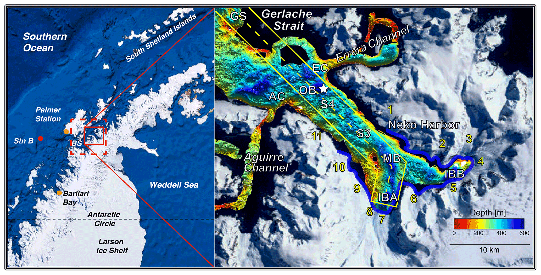
Figure 1Regional map of study region (red box, inset right) and model domain (dashed red box) with nearby Palmer Station, shelf station (Stn B), and Bismarck Strait (BS). Bathymetric map of Andvord Bay with important stations labeled (GS: Gerlache Strait; AC: Aguirre Channel; EC: Errera Channel; OB: Outer Basin; S4: Sill 4; S3: Sill 3; MB: Middle Basin; IBA: Inner Basin A; IBB: Inner Basin B) and the surrounding tidewater glaciers numbered (4: Moser Glacier; 7: Bagshawe Glacier). The locations for sediment cores collected in January 2016 and included in this study are indicated by the star. The dashed yellow line indicates the transect along which vertical sections are plotted. The blue outline (inset right) shows glacial fronts where meltwater is introduced in the model.
A total of 18 stations per season were sampled for Fe geochemical variables using acid-cleaned 12 L Go-Flo bottles (General Oceanics) suspended in series on a clean hydroline (Amsteel) and triggered with acid-cleaned Teflon messengers designed by Ken Bruland (UC Santa Cruz). This sampling effort coincided with concurrent CTD stations. Once on board, Go-Flo bottle tops and bottoms were covered with plastic and placed on a wooden rack located within the trace-metal clean shipboard plastic “bubble”, which was positively pressurized with HEPA-filtered air. Sample bottles were soaked in a soap detergent overnight with heat applied (60 ∘C), followed by a 1-week soak in 3N HNO3 (trace-metal grade) at room temperature and finally a 1-week soak in a 3N HCl (trace-metal grade) bath at room temperature. Rinsing with ultrapure Milli-Q water occurred after each step. Samples for dFe analysis were pressure-filtered (N2 gas, 99.99 %) directly from Go-Flo bottles through 0.2 µm Acropak 200 capsule filters (VWR International) into low-density polyethylene bottles (Nalgene) and acidified to pH 1.7 to 1.8 using HCl (Optima grade, Fisher Scientific). Samples for Fe-binding ligands were similarly filtered in-line but collected in fluorinated high-density polyethylene (Nalgene) bottles, unacidified, and frozen at −20 ∘C until laboratory analysis back on land. This sampling protocol followed established trace-metal clean methods to the standards of the GEOTRACES program to avoid metal contamination. In addition to the filtered samples, unfiltered seawater was sampled directly from the Go-Flo bottles and acidified to pH 1.8 and stored for > 6 months (up to 2 years) and vacuum-filtered prior to analysis using acid-cleaned 0.4 µm polycarbonate (PC) filters in a Teflon filtration apparatus to determine total dissolvable Fe (TDFe). Labile particulate Fe (LpFe) is calculated as the difference between TDFe and dFe. Particulate samples were collected on 0.4 µm PC filters and stored at −20 ∘C until complete digestion using an HNO3–HF mixture. The digestion method employed is described in Planquette and Sherrell (2013) and is widely used in the GEOTRACES program (Cutter and Bruland, 2012; Fitzsimmons et al., 2017) .
Attention to cleanliness was applied when sampling icebergs during small boat deployments in the fjord. Floating icebergs were sampled using a clean stainless-steel pickaxe and rust-free stainless-steel screwdriver and plastic mallet for chiseling pieces of ice. Samples were collected by slowly (engine idled) approaching the target piece of floating ice from downwind, limiting the chance of engine exhaust contamination. Each piece of ice was collected above freeboard (sea surface), to reduce the chance the ice was altered by seawater, and rinsed with Milli-Q prior to placing into acid-cleaned 2 gallon Ziploc polyethylene bags and storing at −4 ∘C until sample processing. Prior to filtration, ice samples were removed from the freezer and left to melt at ambient shipboard temperatures. Once completely melted, a small incision was made on the Ziploc bags using a clean stainless-steel razor, and contents were poured into the Teflon filtration manifold or directly into sample bottles, thus collecting samples for dissolved, total dissolvable, and particulate trace-metal fractions. We note that steel-free tools should be used when available, such as titanium tools and ceramic knives, for the cleanest method for sampling of icebergs.
2.2 Trace-metal concentrations
Stored acidified filtered seawater samples were analyzed for Fe at Scripps Institution of Oceanography using flow injection with chemiluminescence methods described by Lohan et al. (2006). Dissolved Fe in the samples was oxidized to iron(III) for 1 h with 10 mM Q-H2O2 (Suprapur grade), buffered in-line with ammonium acetate to pH ∼ 3.5, and pre-concentrated and matrix removed on a chelating column packed with a resin (Toyopearl® AF-Chelate-650M). Dissolved Fe was eluted from the column using 0.14 M HCl (Optima grade, Fisher Scientific), and the chemiluminescence was recorded by a photomultiplier tube (PMT, Hamamatsu Photonics). The manifold was modified based on Lohan et al. (2006). Standardization of Fe was carried out with a matrix-matched standard curve (0, 0.4, 0.8, 3.2, 10 nmol kg−1 added high-purity Fe metal ICP spectrometry standard in 2 % HNO3) using 0.34 nM dFe Pacific surface seawater. Standards were treated identically to samples. Accuracy was assessed by repeated measurements of GEOTRACES coastal and Pacific Ocean reference seawater samples. Our measurements of GSC gave Fe = 1.391 ± 0.115 nM (n=19, over a 3-month period, consensus 1.535 ± 0.115 nM). Our measurements of GSP gave Fe = 0.164 ± 0.024 nM (n=8, over a 1-month period, consensus 0.155 ± 0.045 nM). Consensus values are from the most recent July 2019 compilation (geotraces.org). Precision, determined by replicated analyses of an in-house large-volume reference seawater sample within each analytical session, was typically ± 5 % or better. For the duration of these analyses, the average limit of detection (defined as 3× the standard deviation of the blank) was 0.036 nM dFe (n=10).
A subset of the seawater samples and all freshwater samples were run for Fe and Mn at Rutgers University using isotope dilution inductively coupled plasma mass spectrometry (ICP-MS) methods based on Lagerström et al. (2013) and similar to those described in Annett et al. (2017). Briefly, 10 mL aliquots of seawater samples were extracted using a commercially available automated SeaFAST pico system (Elemental Scientific, Inc.) after online buffering to a pH of approximately 6.5 using ammonium acetate buffer, achieving a 25-fold pre-concentration after column elution in 0.4 mL of 1.6 M ultrapure nitric acid (Optima grade, Fisher Scientific)(Lagerström et al., 2013). Isotope dilution was used to standardize Fe, while Mn was standardized using an external matrix-matched standard treated identically to samples. The analysis of the concentrate was performed on an Element 2 sector-field ICP-MS (Thermo Fisher Scientific). Accuracy and precision (± 3 %, 1SD, for Fe and Mn) were assessed by repeated measurements of in-house large-volume reference seawater samples within each analytical session. Blanks averaged 51 pmol kg−1 for Fe (n=59; limit of detection, or LOD = 48 pmol kg−1) and 4 pmol kg−1 for Mn (n= 69; LOD = 4 pmol kg−1) for all analytical runs. A comparison of the seawater analysis methods employed here is shown in Fig. S1. In general, there is good agreement (average 11 % and 6 % difference between late spring and fall, respectively) between the chemiluminescence and ICP-MS methods, comparable to the uncertainty of GEOTRACES consensus values from the intercalibration of 13 trace-metal laboratories (for Fe, RSD 10 %, https://www.geotraces.org/standards-and-reference-materials/, last access: 1 March 2021). Total dissolvable trace metals and particle digests, including freshwater dissolved metals (i.e., glacial melt), were analyzed using direct-injection ICP-MS methods using external standards and added In as a matrix and instrument drift corrector for the quantification of particulate Fe, Mn, aluminum (Al), and titanium (Ti) concentrations (Annett et al., 2017).
2.3 Sediment cores and diffusive flux
Cores for this study were collected using a 12-barrel Megacore multi-coring device aboard the R/V Nathaniel B. Palmer cruise NBP16-01 in January 2016. Multiple barrels were sampled from a single Megacore deployment. See Taylor et al. (2020) for a complete account of coring efforts and Komada et al. (2016) for a description of the pore water sampling procedures. Porewater dFe and dMn were determined colorimetrically using the ferrozine and formaldoxime techniques, respectively (Armstrong et al., 1979; Burdige and Komada, 2020). For dFe, hydroxylamine-HCl (0.2 % final concentration) was added to the samples before analysis, to reduce any dissolved Fe(III) in the samples to Fe(II). For dMn, a hydroxylamine solution was added to an acidified (pH ∼ 1–2) sample, and an EDTA solution was added to remove interference from a colored Fe complex. Porewater oxygen concentrations were measured using a polarographic microelectrode (Brendel and Luther, 1995; Luther et al., 1998, 2008). A sequential extraction technique (Goldberg et al., 2012; Poulton and Canfield, 2005) was used to determine sediment Fe speciation for the following fractions: Feox (highly reactive, poorly crystalline iron oxides), Femag (magnetite), Feprs (Fe in poorly reactive sheet silicates), FeT (total sediment Fe), Fepyr (Fe in pyrite), and finally FeU (unreactive pool under all treatments = FeT − (Feox+ Femag+ Feprs+ Fepyr)). All extracts were analyzed for Fe by flame atomic absorption spectrometry (for details see Burdige and Komada, 2020).
In this study, we investigate the potential for efflux of dissolved trace metals as a source to the overlying water column. Using Eq. (1), we can estimate the approximate sediment diffusive flux (Jsed) for dissolved porewater species.
In this equation, ϕ is the porosity of the sediments and was found to be 0.9 on average near the sediment surface. Porewater analyses of dissolved Fe and Mn in the Outer Basin (OB) cores reveal high variability in the top-of-core gradient () in porewater Fe and Mn (Fig. S2). An average of two cores gives a gradient of 21.9 µM cm−1 dissolved Fe and 3.6 µM cm−1 dissolved Mn. Assuming a diffusion coefficient for Fe and Mn in free solution for seawater (DSW) at 0 ∘C to be 3.15x10⁻¹⁰ m2 s−1 for Fe(II) and 3.02 × 10⁻¹⁰ m2 s−1 for Mn(II), we can then estimate the diffusion coefficient in the sediments (Dsed) using the following relationship (Boudreau, 1996; Halbach et al., 2019):
2.4 Iron-binding ligands
A subset of seawater samples was analyzed for dFe-binding ligands using single analytical window methods. The methods applied here are described extensively in Buck et al. (2018). Briefly, natural seawater samples were titrated with dFe (0–35 nM) in order to fully saturate the natural ligands. Following a 2 h equilibration with the added Fe, a well-characterized ligand (salicylaldoxime, SA) was added to compete with natural dFe-binding ligands. The concentration of SA used in this study to examine ligands was 25.0 µmol L−1 (). After at least 15 min of equilibration, the Fe(SA)x electroactive complex was measured using adsorptive cathodic stripping voltammetry (ACSV) on a hanging mercury drop electrode (BioAnalytical Systems, Incorporated). Peak heights were measured using ECDSOFT, and sensitivity was optimized in ProMCC (Omanović et al., 2015). A combination of traditional linearization techniques was previously applied to determine the concentrations and strengths of natural ligands within the seawater sample using ProMCC (Omanović et al., 2015). The uncertainty on modeled complexation parameters was optimized using single- or multiple-ligand fitting. These methods were applied successfully to the GEOTRACES speciation data sets (Buck et al., 2015, 2018).
We calculate the capacity for the free ligand pool to bind Fe at equilibrium (Fitzsimmons et al., 2015), or , defined as
where eL is the difference between the total ligand concentration (Lt) and the dFe concentration, and K is the conditional stability constant.
2.5 Numerical model simulations
Based on Hahn-Woernle et al. (2020), the ocean in the Andvord Bay region is modeled with the primitive-equation, finite-difference Regional Ocean Model System (ROMS; Haidvogel et al., 2008). The grid has a horizontal resolution of ∼ 350 m and a terrain-following vertical coordinate system with 25 depth layers. Due to the changing terrain, the fixed number of layers, and surface intensified resolution, the maximum thickness for deeper layers is 84.6 m, and the minimum thickness for surface layers is 0.5 m (to better resolve the surface currents, for example). The domain has three open boundaries: the western end of Bismarck Strait, a passage to the continental shelf in the northwest, and along Gerlache Strait to the northeast (Fig. 1). Boundary and initial conditions were derived from CTD and ADCP observations. The model is forced with tidal and meteorological data (from TPXO8 Egbert and Erofeeva 2002 (updated) and RACMO van Wessem et al., 2014, respectively) and run from November 2015 for 5 months. After 1 month, the transient effects, based on dynamics and thermodynamics, were found to no longer be present, and the system was consistent. Only the final 4 sea-ice-free months were analyzed (December through March). Processes like melting of icebergs and floating sea ice are not modeled directly; therefore such local freshwater sources are represented in a surface intensified meltwater input applied along the glacial fronts (for further details see Hahn-Woernle et al., 2020). These new freshwater sources also include surface runoff and local melt of glacial ice, while precipitation and snowfall are represented in the meteorological forcing. To represent the seasonal cycle of temperature-induced melting, the volume flux of inflowing meltwater follows a bell-shaped temporal distribution peaking at the end of January.
We use this model to identify the potential supply pathways and estimate the hydrographic export of three Fe-rich sources in Andvord Bay: surface glacial meltwater, subsurface subglacial plume, and deep water masses located within the inner basin. For this purpose, we designed three model experiments with numerical “dyes” to track potential iron pathways: one, to track the current seasonal input of meltwater from glaciers in Andvord Bay (surface meltwater dye experiment) released along the glacial fronts in the inner fjord at 0–50 m depth (Fig. 1), and two additional experiments involving subsurface water masses in front of Bagshawe Glacier in Inner Basin A (IBA, 64∘53′36′′ S, 62∘34′48′′ W) at two different depths (subsurface and deep dye experiments). Due to the model geometry, the mean depths at which the subsurface and deep dyes were released were 107 (94–120 m) and 314 m (290–342 m), respectively. Covering two horizontal grid cells each (with different thickness), the subsurface and deep dyes had initial volumes of 5 × 10⁶ and 11.3 × 10⁶ m3, respectively. It follows from the experiment setup that the surface meltwater dye has a continuous source while the total amount of the other two dyes is a constant as long as they do not leave through the open boundaries of the model domain.
3.1 Seasonality and hydrography in Andvord Bay
In Andvord Bay (Fig. 1), seasonal changes in phytoplankton biomass were documented, as indicated by the proxy chlorophyll a, which shows a 10-fold concentration decrease across all taxonomic classes between the late spring and fall cruises (Pan et al., 2020). Associated with these changes in primary production, depletion of the surface macronutrients nitrate (N) and silicic acid (Si) were observed (Ekern, 2017). Increased Si concentrations, with respect to nitrate, within the inner fjord are driven by dissolution of biogenic silica sediments, or weathering of the bedrock by contact with the 11 marine-terminating glaciers feeding into Andvord Bay since Si-to-N ratio is highly correlated with meltwater fraction (MWf) below the surface layer (Hawkings et al., 2018; Ng et al., 2020). Surface stocks of macronutrients were never exhausted (Fig. 2). The phytoplankton community was dominated by small size classes, with very few large diatoms (Pan et al., 2020). The microplankton class, including large diatoms, was sparingly present in the fall; however, benthic cameras captured a large sedimentation event of marine aggregates indicative of a large diatom bloom in late January. The export of biogenic particles from the surface also showed a distinct seasonality indicated by increased chlorophyll a pigment content in seafloor surface sediments in fall (Ziegler et al., 2020), as well as higher respiration rates from chamber incubation experiments in the fall compared to spring (data not shown), although no indication of sulfate reduction was observed in sediment box and Kasten cores (2.3 m long), suggesting that oxygen, nitrate, and metal oxides were sufficient to oxidize organic matter within the upper sediments (Craig Smith, personal communication, 2018).
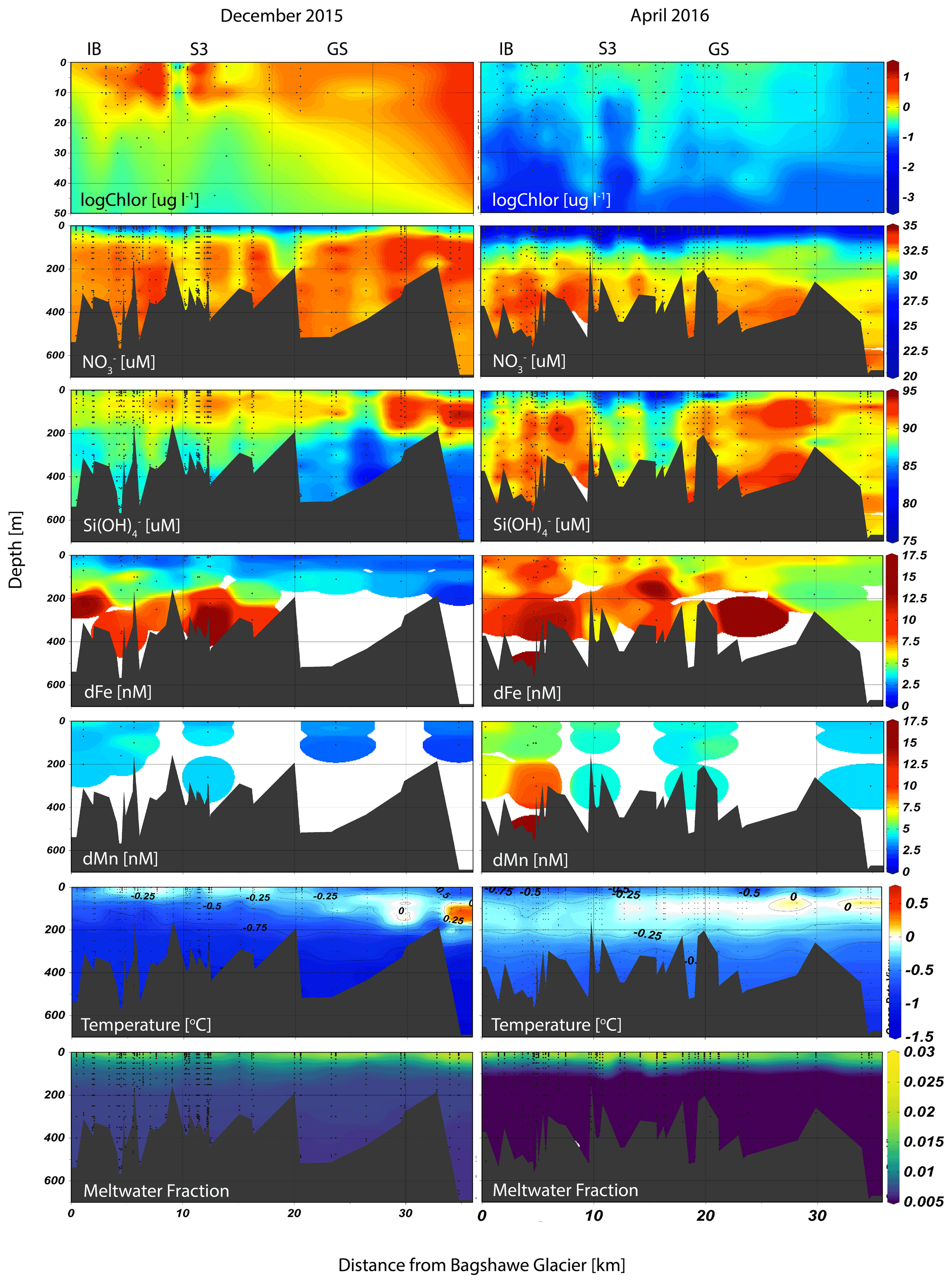
Figure 2Seasonal phytoplankton, macronutrient, micronutrient, temperature, and meltwater distributions plotted as sections extending from the inner basin (IB, left) towards Gerlache Strait (GS, right). Plots were made with Ocean Data View visualization software (Schlitzer, 2002, Ocean Data View, last access: 1 February 2021).
Derived glacial MWf (Fig. 2), based on salinity and oxygen isotopes of seawater, ranged from 0.75 %–2 % in late spring and from 0.5 %–2.5 % in the fall (Pan et al., 2019). The fjord also exhibited a gradient in meltwater content, with the highest MWf at the glacier terminus. Using a simple mass balance for the surface layer in Andvord Bay, we estimate an approximate meltwater input of 23 600 m3 d−1 in order to account for the observed changes in oxygen isotope ratios. This estimate is within the derived estimates of surface meltwater flux generated by warm atmospheric temperatures (1.4 × 10⁴ to 1.2 × 10⁵ m3 d−1; Lundesgaard et al., 2020). The MWf is strongly correlated with phytoplankton abundance within Andvord Bay; for a detailed discussion see Pan et al. (2019). We find that glacial meltwater impacts phytoplankton within the fjord, but the geographical influence of meltwater can extend across the shelf, hundreds of kilometers from the coastal inputs (Dierssen et al., 2002; Meredith et al., 2017).
Physical properties measured in the study region showed the dominant water masses in the fjord were Antarctic Surface Water (cold fresh) and Bransfield Strait water (cold salty) (Lundesgaard et al., 2020). However, during late spring, greater influence of modified Upper Circumpolar Deep Water was observed outside of the fjord, indicated by its distinctly higher temperature at depth, but this water mass is prevented from entering the fjord due to a shallow sill near the fjord mouth in the Gerlache Strait (Fig. 2). Optical measurements recorded a change in the particle concentration and assemblage between the two cruises. Profiles of beam attenuation coefficient and particulate backscattering coefficient showed strong seasonality (see Fig. 4 and discussion in Pan et al., 2019). Pan et al. (2019) interpreted these optical signatures in the upper water column as a change from a surface biogenic-dominated signal in late spring to a subsurface lithogenic-dominated signal in the fall, composed of fine suspended particles contained within plumes. An important feature observed within the fjord was a subsurface neutrally buoyant plume (∼ 100 m) characterized by a point source of relatively cold and particle-laden water emanating from the terminus of Bagshawe Glacier and extending several kilometers over the inner basin (Fig. S3).
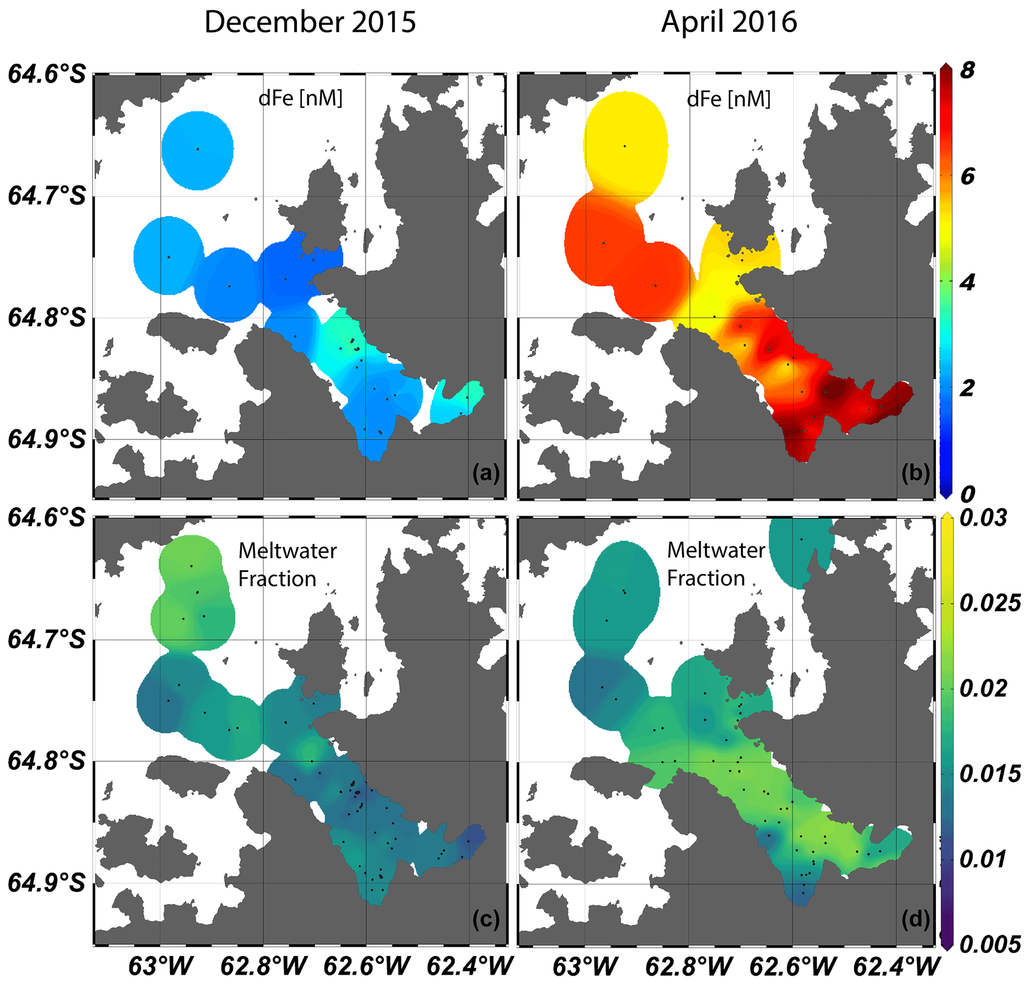
Figure 3Surface (< 20 m) dissolved Fe (a, b) and meltwater fraction (c, d) for late spring (left two panels) and fall (right two panels). Plots were made with Ocean Data View visualization software (Schlitzer, 2002, Ocean Data View, last access: 1 February 2021).
Strong buoyant plumes can drive circulation in fjords via the “meltwater pump”, but small amounts of basal and subglacial melt have a negligible effect on circulation in Andvord Bay. While this process is described in depth for Arctic glaciers, Andvord Bay differs in that ocean temperatures are approximately −1 ∘C at depth, too cold to ablate the glacier terminus, and neutral buoyancy is reached below the surface layer (indicated by subsurface sediment plumes; Domack and Ishman, 1993). However, cold-water glaciers must have some mass loss even at seawater temperatures below the glacial ice melting point. Two important consequences of these plumes are a flux of suspended particulate matter within subsurface “layers” as indicated by a high beam attenuation coefficient and optical backscatter (Fig. S3 in Pan et al., 2019), and general mid-water cooling found in the inner fjord (Fig. 8 in Lundesgaard et al., 2020). Downstream mixing mechanisms, such as flow over topographic features or wind-induced upwelling, can displace plume water closer to the euphotic zone.
3.2 Water column trace metals
Dissolved Fe concentrations in the surface, defined as the upper ∼ 20 m based on similar mixed layer depths (MLDs) for both seasons (Lundesgaard et al., 2020), changed seasonally with an overall increase in dFe concentration in the fall (Fig. 3). The average surface concentration during late spring was 2.47 ± 0.92 nM (n=21), while in fall it was 6.67 ± 1.41 nM (n=19). Water column trace metals are presented in Table S1. These concentrations are within the ranges of dFe determined in prior studies (1–31 nM) in the northern WAP region but indicate that large temporal variability exists in surface waters in this region (Bown et al., 2018; Hatta et al., 2013; Sañudo-Wilhelmy et al., 2002; Ardelan et al., 2010; Martin et al., 1990). The smaller range of surface concentrations during late spring suggests that dFe was more tightly controlled by phytoplankton uptake, whereas in the fall, patchiness among stations arises due to varying proximity to Fe sources and the effects of circulation and mixing. Vertical profiles of dFe showed a steep increase to values greater than 10 nM at the deepest depths sampled during late spring, especially at stations located within the inner fjord and basins (Figs. 2, 4). In the subsurface (50–150 m), an enriched dFe source was present with average concentrations 3.68 ± 1.52 nM in late spring and 7.38 ± 2.49 nM in the fall. Deep water masses more than 150 m deep had the highest average concentrations of dFe, and similar mean concentrations were observed for both seasons (8.79 ± 4.75 nM in late spring, 6.37 ± 2.38 nM in fall). The greatest concentrations of dFe were found in the inner fjord and basin stations, with the exception of one station located at the mouth of the fjord near Aguirre Channel (station AC in Fig. 1). Water column concentrations were lower in the Gerlache Strait and fjord mouth. The general shapes of the profiles in late spring are characteristic of a stratified water column, with dramatic ferriclines below the surface.
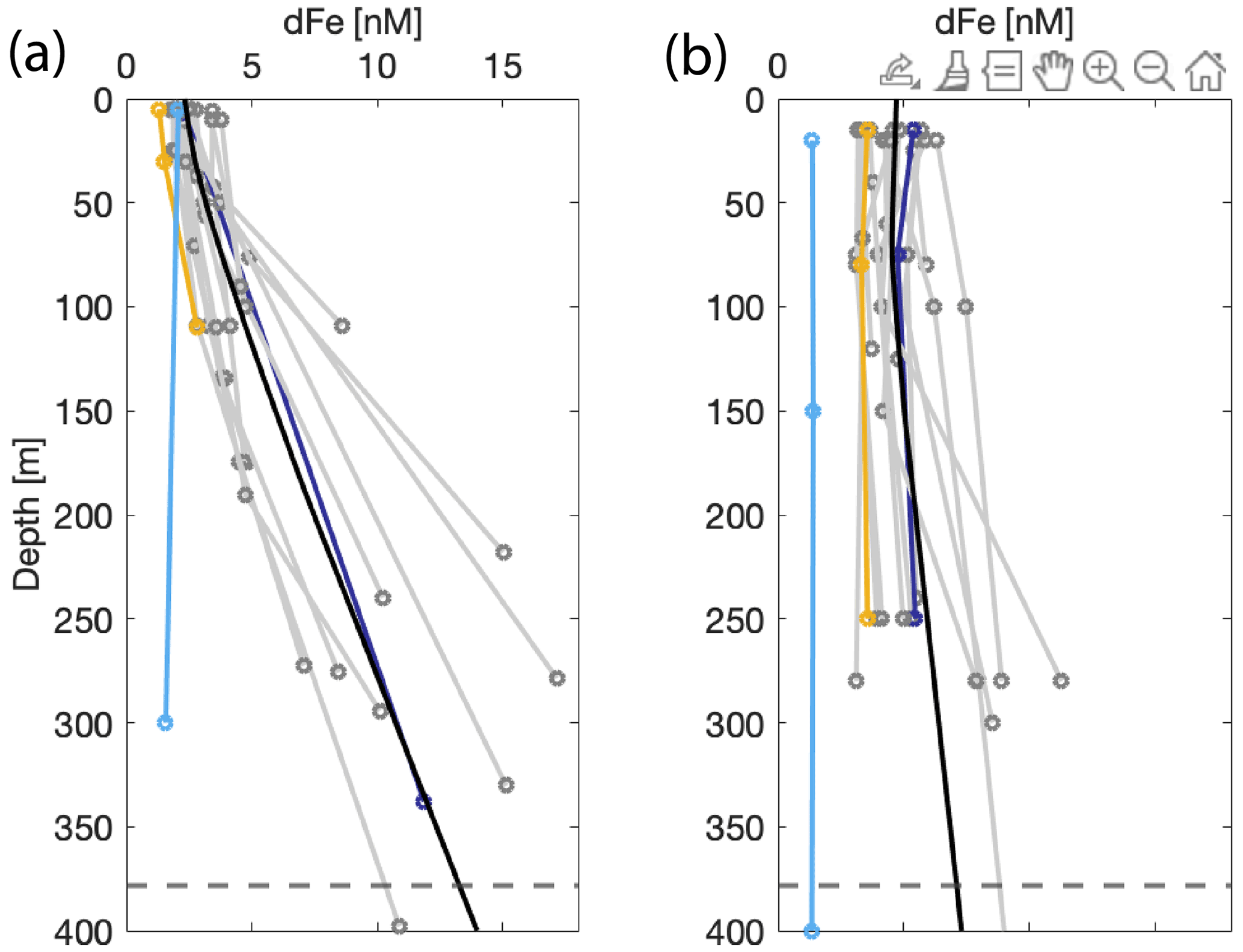
Figure 4Depth profiles of dissolved Fe [nM] sampled in the Andvord Bay region for December 2015 (a) and April 2016 (b). The colored lines indicate highlighted profiles: the geometric mean of the linearly interpolated data points within Andvord Bay (black), Station B on the continental shelf (light blue; see Fig. 1), Station GS (Gerlache Strait, yellow), and Station S3 (dark blue). Other Andvord Bay stations are shown in grey. The dashed line is the average bottom depth within the fjord.
In the fall, surface dMn was more than double that observed in late spring, but surface dFe showed a greater seasonal increase, such that the dissolved Mn : Fe ratio decreased overall and was more variable than in late spring. Concentrations of dMn remained below 4.5 nM, even at depth in the late spring. Labile particulate Mn (LpMn = TDMn − dMn) showed strong co-variation with LpFe and beam attenuation coefficient c(660). The comparatively high surface dissolved Mn : Fe ratios in late spring were presumably due to intense biological drawdown of Fe during the vernal bloom, evidenced from low concentrations of dFe where phytoplankton biomass (as chl a) was highest (Fig. 5a). In the late spring, dFe is anti-correlated with MWf (Fig. 5c), whereas there was no significant trend between dFe, biomass, and MWf variables in the fall (Fig. 5b, d). The correlation between dMn and dFe was stronger in the fall, however, compared to the late spring (Fig. 5e, f).
Labile particulate iron (LpFe = TDFe − dFe) concentrations were elevated in the inner basins in late spring and fall and strongly correlated with suspended particle concentrations, indicated by optical beam attenuation coefficient c(660) m−1 (Fig. 5n). Average TDFe and LpFe concentrations in the surface were comparable to surface waters in Ryder Bay (southern Antarctic Peninsula), where TDFe varied temporally from 57 to 237 nM (Annett et al., 2015). This comparison between LpFe and TDFe is valid since TDFe is much greater than dFe in these two coastal locations; hence it is a good approximation of LpFe. The LpFe maxima were associated with high turbidity in the inner basins, reaching as high as 900 nM at 300 m depth in the fall (Fig. 6). Dissolved Fe and LpFe were correlated (r2=0.48 late spring n=19; 0.77 fall n=28) (Fig. 5g, h). On average, dFe made up 3.1 % (late spring) and 4.6 % (fall) of the total dissolvable pool. The LpMn concentrations displayed similar seasonality to LpFe and a similar association with total particles, but they were more strongly correlated in the fall (Fig. 5l). Dissolved Mn and LpMn were highly correlated (r2=0.70 late spring n=19; 0.79 fall n=28; Fig. 5i, j). On average, dMn composed 52 % (late spring) and 57 % (fall) of the total dissolvable pool.
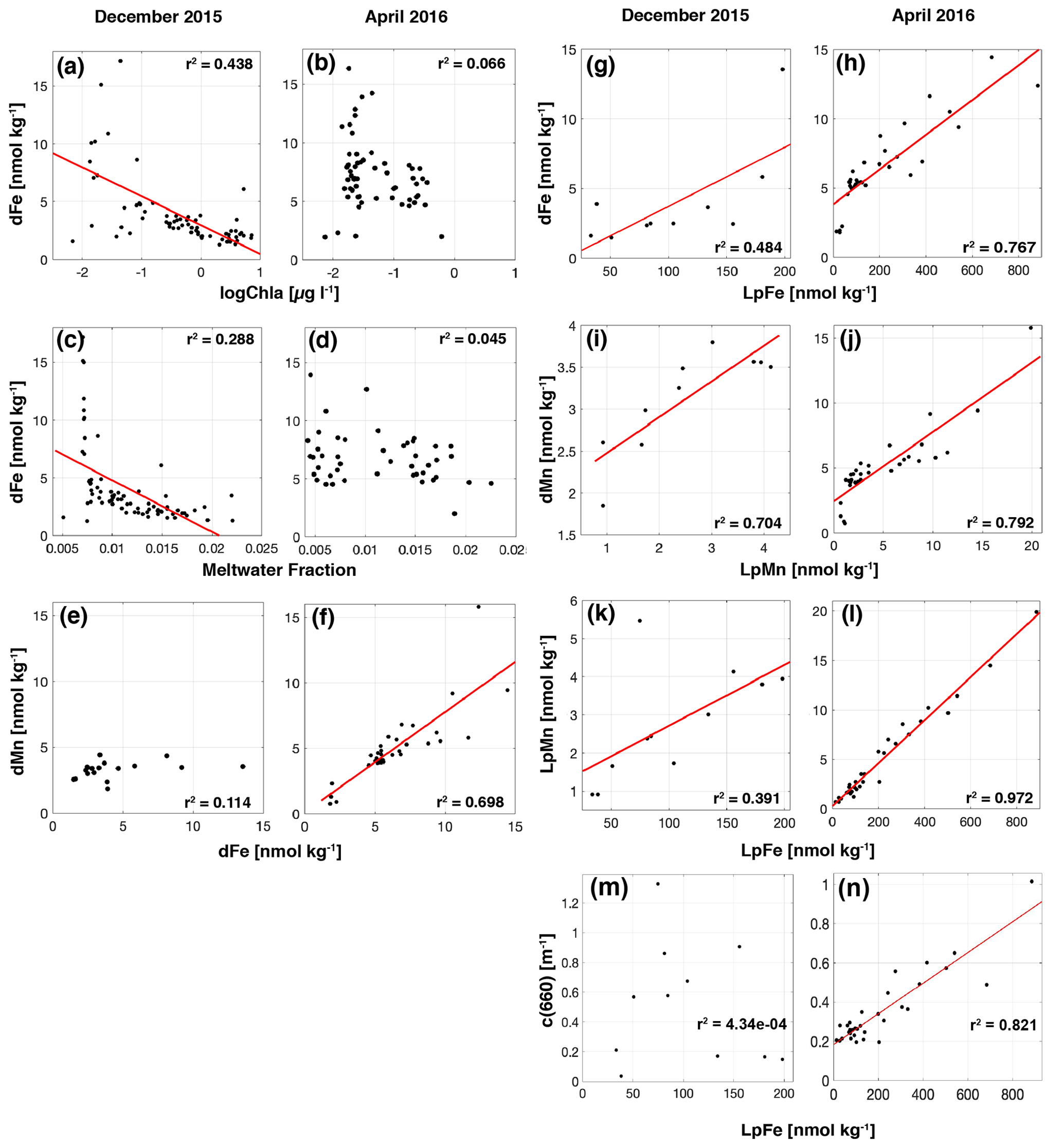
Figure 5Dissolved trace metals plotted against observed and derived variables for December 2015 (a, c, e) and April 2016 (b, d, f). Dissolved Fe (a–b) versus logChlorophyll a concentrations. Dissolved Fe (c–d) versus meltwater fraction. Dissolved Mn (e–f) versus dissolved Fe. Least-squares regression lines are shown where they are statistically significant (p<0.005).
Figure 5 (continued). Dissolved Fe and Mn concentrations versus labile particulate Fe and Mn for each season. Dissolved Fe (g–h), labile particulate Mn (k–l), and beam attenuation coefficient (m–n) versus labile particulate Fe. Dissolved Mn (i–j) versus labile particulate Mn. Least-squares regression lines are shown where they are statistically significant (p<0.005).
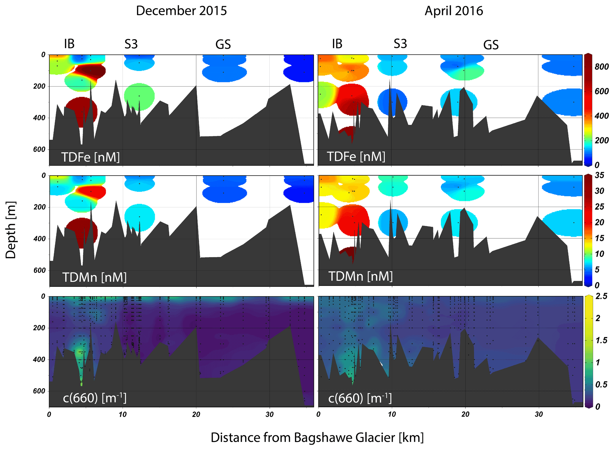
Figure 6Total dissolvable trace metals and beam attenuation coefficient c(660) for both seasons. The transects are plotted as distance from the Bagshawe Glacier terminus. Plots were made with Ocean Data View visualization software (Schlitzer, 2002, Ocean Data View, last access: 1 February 2021).
3.3 Glacial ice and plume trace metals
Glacial ice and plume samples were analyzed for Fe, Mn, Al, and Ti concentrations, which are presented in Table 1. Three glacial ice samples were analyzed for dFe (72 ± 121 nM) and dMn (49 ± 83 nM). Visual inspection of Glacial Ice 3 and 4 showed these pieces contained low particle loads, while Glacial Ice 1 and 2 had a comparatively high content of dark colored coarse-grained particles. Hence, these and the “clean” glacial ice samples are indicative of the variability of trace-metal concentrations in icebergs found in Andvord Bay. Labile particulate trace-metal concentrations were 2 orders of magnitude higher than the dissolved fraction based on two ice samples (41 ± 86 µM LpFe, 3.6 ± 5.1 µM LpMn). We did not determine labile particulate trace metals for Glacial Ice 3 and 4; thus these average labile particulate concentrations are skewed toward a high value. Total particulate trace metals showed similar concentration variability to the dissolved fraction (95 ± 181 µM TpFe, 2.7 ± 5.1 µM TpMn). For Glacial Ice 3 and 4, the concentration of dMn was greater than TpMn. The ratios of labile and total particulate Mn : Fe were 0.061 ± 0.002 mol : mol and 0.028 ± 0.004 mol : mol, respectively.
Dissolved Al and Ti were not analyzed for these ice samples, but total dissolvable and total particulate samples were analyzed for Glacial Ice 1 and 2 and 1–4, respectively. We defined the refractory particulate trace-metal concentration as the difference between the total particulate and total dissolvable fractions (RpTM = TpTM − TDTM). Total dissolvable Al and Ti average concentrations were skewed due to the heavy particle load present within Glacial Ice 1 and 2 (603 ± 716 µM TDAl, 20.8 ± 27.1 µM TDTi). Total particulate Al and Ti had similar variability to the total dissolvable fraction and included all four glacial ice samples with averages of 428 ± 790 µM TpAl and 13.4 ± 25.7 µM TpTi; therefore the average total particulate concentrations were lower than the average determined for total dissolvable Al and Ti in Glacial Ice 1 and 2. We found the labile particulate concentration to be a valid comparison to total dissolvable particulate concentration since dFe concentration was on average 1.8 ± 1.5 % of TpFe concentration. Thus, the particulate fraction dominated trace-metal speciation of total Fe, Mn, Al, and Ti in glacial ice.
Table 1Glacial ice and seawater samples analyzed for dissolved, labile, and total particulate trace metals. Crustal averages from Taylor and McClellen (1995): Mn : Fe (0.017 mol : mol), Fe : Al (0.2), and Al : Ti (35).

NA: not available.
Four seawater samples were collected from 100–110 m depth, corresponding to the core of the subsurface turbidity plume within IBA. Average concentrations of dissolved metals were 8.75 ± 2.25 nM dFe and 5.52 ± 0.62 nM dMn. LpFe (351 ± 148 nM) and LpMn (8.23 ± 2.68 nM) were indistinguishable from the total particulate fractions (416 ± 93 nM TpFe, 9.52 ± 2.05 nM TpMn) within measurement error, including filter splitting and sample distribution uncertainties. The average ratio of labile particulate Mn : Fe was 0.024 ± 0.003 mol : mol. Particles collected from the plume had high concentrations of Al and Ti but with distinctly different lability from that of Mn and Fe. The TDAl was 894 ± 68 nM while TpAl was 1734 ± 369 nM. Similarly, TDTi was 14.1 ± 0.45 nM and TpTi was 45.1 ± 10.7 nM. The total dissolvable Al : Ti ratio was 64 ± 6 mol mol−1 and the total particulate Al : Ti ratio was 39 ± 1 mol mol−1. The Al : Ti ratio is elevated above the crustal ratio (35 mol mol−1) in the total dissolvable fraction, suggesting a larger adsorbed fraction for Al than for Ti.
3.4 Glacial sediments
Solid phase Fe speciation of one sediment core from the Outer Basin station (OB, 64∘46′46′′ S, 62∘43′57′′ W, ∼ 500 m, collected in January 2016) showed an enrichment of authigenic Fe oxides at the surface. Chemical treatments of the sediments with HCl poorly dissolves crystalline Fe oxy(hydr)oxides (ferrihydrite and lepidocrocite), which are found to be 10 % of the total particulate Fe of the surface sediments in this location, compared to an average of 2 % below 1.5 cm (Fig. S4). In the surficial sediments, a larger portion of the Fe is associated with poorly labile sheet silicates (e.g., structural Fe(III) in clays, 36 %), and a comparable fraction is refractory and is not liberated by any of the solution treatments (31 %). Other fractions of particulate Fe are associated with more crystalline Fe oxides (goethite, hematite) and the minerals magnetite and pyrite. Porewater analyses were performed on two OB cores using colorimetric methods, revealing high concentrations of dFe and dMn. Below the well-oxygenated layer (upper ∼ 0.5 cm), but within the upper 10 cm, dFe reaches its peak concentration of 80 µM, while maximum dMn is 6 µM. Down-core from the peak, concentrations tend to decrease for both trace metals, but there is considerable variability between 15 and 25 cm, including several deeper local maxima. The average porewater concentration of dFe in the top 2.5 cm is 26 µM (Fig. S2). There is considerable difference in the porewater concentrations of the two OB cores, indicating bioturbation of the sediments resulting in large variability on small scales. Points excluded from the oxygen profiles were below the detection limit, while several samples were lost from the porewater profiles, represented as gaps in the vertical traces of dFe and dMn.
3.5 Fe-binding organic ligands
To gain insight into the speciation of dFe within the fjord, we analyzed seawater samples for Fe-binding ligands and to identify comparative strengths of organic Fe complexes (see Sect. 2). There is potential to overestimate ligand concentrations using these methods (Gerringa et al., 2021); however, the trends within these data and interpretations are valid. Analysis of the ligands within Andvord Bay shows a down-fjord gradient in both quantity and quality (all ligand data presented in Table 2). In the late spring, strong ligands ) were detected in the surface at stations located within the fjord at concentration levels ranging from 4.06 ± 1.74 nM at Inner Basin A (IBA) to 7.27 ± 1.97 nM at Sill 3 (S3), while only weak ligands () were detected in the Gerlache Strait (GS; 5.72 ± 2.21 nM). An excess of strong ligands, relative to dFe, was detected in the inner basins. A gradient in concentration of undersaturated ligands (eL in Table 2) is observed towards the GS, with increasing eL. Within the fjord, weak ligands were detected at Inner Basin B (IBB), closest to Moser Glacier. In the fall, total ligand concentrations (Lt) were elevated everywhere within the fjord, but the surface ligands were somewhat weaker compared to the late spring. The greatest concentrations of ligands were found closest to the glaciers (range 11.18–15.42 nM) and in the GS (12.00 ± 2.94 nM). For both seasons, weak ligands were detected in the subsurface, but a greater concentration in the fall suggested that these ligands have a local source within the fjord. Compared to other stations in the fall, we found the plume to contain a small excess of weak ligands (IBA, 110 m). Interestingly, the highest concentration of strong ligands (17.44 ± 1.12 nM) among all sites was in deep water of Station IBA, at 280 m. This is the deepest depth sampled for Fe-binding ligands, and the IBA bottom depth was 382 m. We found a down-fjord gradient in ligand strength at the surface, decreasing with distance from the inner basins ( at IBA, 11.03 at GS).
Table 2Ligand concentrations and equilibrium constants detected in seawater samples. Fe′ is the free (unbound) iron concentration. Lt is the total ligand concentration. logK is the conditional stability constant. eL is the excess ligand concentration (eL = Lt − [dFe]). log is the complexation capacity. is the ratio of Fe′ of reoccupied stations, expressed as a percentage.
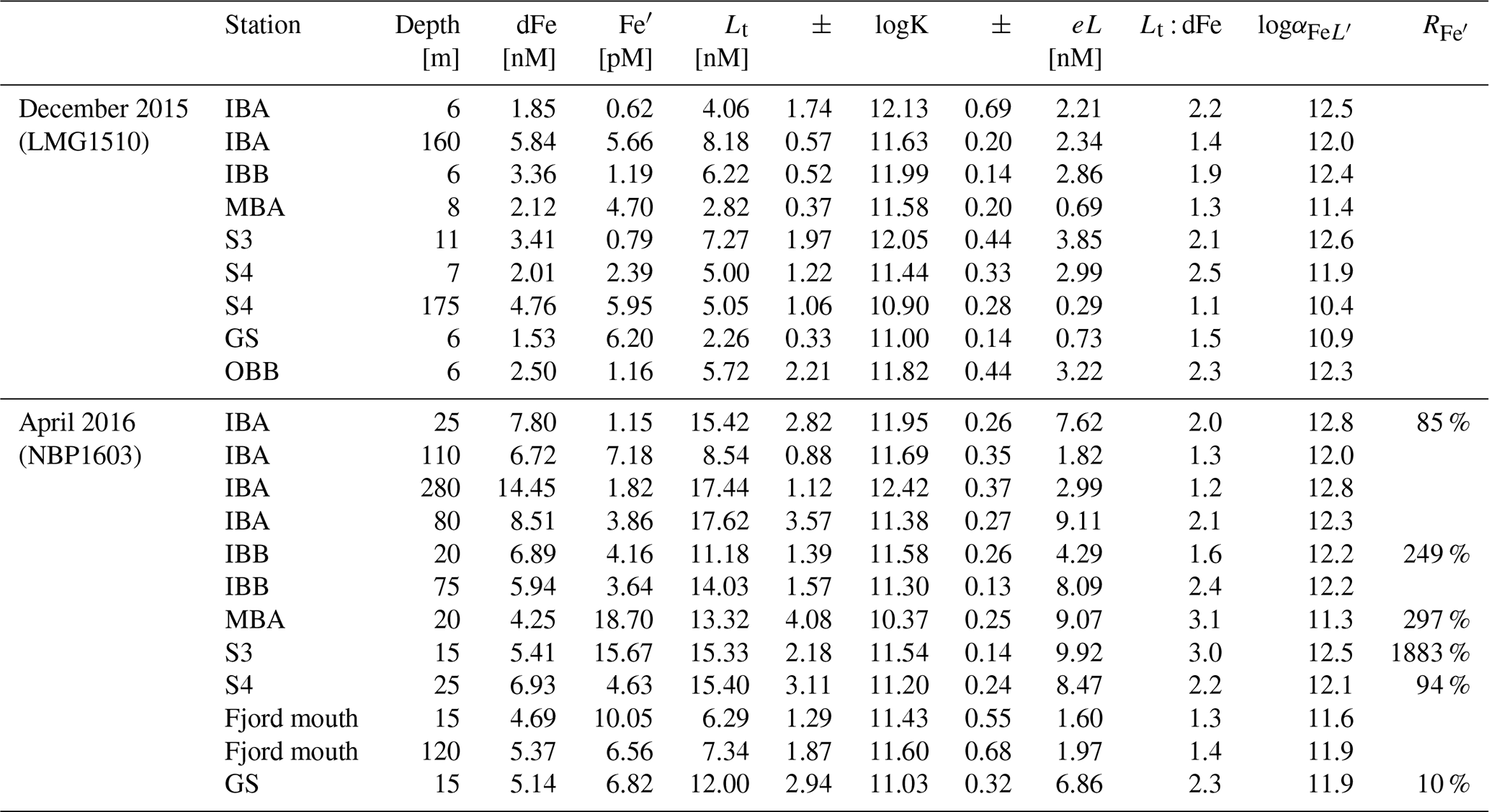
We determined the free (uncomplexed) Fe concentration (Fe′ in Table 2) within samples analyzed for Fe-binding ligands. In the surface, a greater mean concentration of Fe′ was found in the fall (8.74 ± 6.43 pM, n=7) compared to the late spring (2.44 ± 2.18 pM, n=7). Water below the surface showed similar concentrations for each season (5.8 ± 0.21 pM late spring, 4.61 ± 2.22 pM fall). The greatest concentrations of Fe′ were observed mid-fjord at the surface (18.7 pM Fe′ at MB, 15.67 pM Fe′ at S3) in the fall.
3.6 Dye experiments
To study the transport pathways for dFe, we use numerical passive dyes in the Hahn-Woernle et al. (2020) regional model of Andvord Bay (see Fig. 1 in Hahn-Woernle et al., 2020) to track three potential sources of dFe: surface glacial meltwater (0–50 m) from Bagshawe and Moser Glacier termini, neutrally buoyant subsurface plume (100 m), and deep water located in IBA (300 m; as in Methods). Due to numerous inputs and complex biogeochemical processes which result in observed dFe distributions in time and space, we simplify the problem by assuming no removal over the duration of simulated dye experiments. We use this approach to illustrate the multiple transport pathways for dFe supply to the fjord and surrounding ocean from December through March (St-Laurent et al., 2017). The results are presented first for the surface meltwater experiment, followed by two fixed-volume experiments, referred to as subsurface and deep dye experiments.
Most of the surface glacial meltwater dye remains in the upper 100 m throughout the model run, and due to its proximity to the surface, it is quickly dispersed over a large region by relatively rapid surface currents. It takes about 10–15 d for the surface meltwater to exit the fjord mouth, where most ends up in the central and northern Gerlache Strait after 120 d (Fig. S5a).
The subsurface dye (100 m) is spread more rapidly than the deep dye (300 m). After 8 d, the subsurface dye reaches the fjord mouth, which is 4 d before the deep dye, implying it has a shorter residence time within the fjord compared to the deep dye. We loosely define residence time as the model timestamp at which a fixed fraction of dye remains within the fjord domain. After 22 d, 25 % of the subsurface dye has left the fjord, while it takes the deep dye almost twice as long (43 d). At the end of the 120 d long model run, less than 18 % of the subsurface dye and over 30 % of the deep dye remain in the fjord domain (Fig. S6a). Looking at the whole model domain in Fig. 1, which includes Andvord Bay and Gerlache Strait, only 59 % of the subsurface dye and 75 % of the deep dye are still present after 120 d. The missing 41 % (25 %) has mainly left the model domain through the Gerlache Strait to the north, where these waters mix with Bransfield Strait water and subsequently with the southern Antarctic Circumpolar Front waters.
We analyzed the vertical distribution of the subsurface and deep dyes along the fjord mouth and horizontally over different depth layers. Within the first day, the subsurface dye spreads over the depth range of 20 to 125 m and the deep dye over 125 to 500 m (> 1 % of dye per depth layer). The subsurface dye leaves the fjord mainly within the upper 200 m. After 8 d, as the subsurface dye reaches the fjord mouth (Fig. S5b), the maximum concentration is still found close to its release depth at 100–125 m. Over the next few days, surface layer concentrations (< 20 m) increase, but the highest concentration is soon found below 125 m (after 2 weeks) (Fig. S6a).
The deep dye remains mainly below 200 m as it passes the fjord mouth (maximum water depth at the fjord mouth is 360 m). After 12 d, as the deep dye reaches the fjord mouth, the maximum concentration is found below 300 m depth. In contrast to the subsurface dye, the deep dye remains longer in the proximity of the fjord mouth and on several occasions re-enters the fjord, leading to a longer residence time within the fjord (Fig. S5c). The majority of the deep dye leaves the fjord at depths below 100 m and along the southwestern coastline. Both dyes, subsurface and deep, have low concentrations in the upper 100 m of the northeastern flank of the fjord mouth. This is due to the inflow of external water from the GS along the northeastern coastline. Throughout the run, the deep dye is confined to the inner basins of the fjord. In all cases, the dyes remain at higher concentrations and for longer periods in the subsurface fjord waters than in the surface layer, which shows faster transport out of the fjord.
4.1 Iron sources in a heavily glaciated fjord
Due to the proximity to glaciers and influence of ice within Andvord, we hypothesized meltwaters to be an important source of Fe. We focus on quantifying dissolved, total dissolvable and particulate Fe and Mn, as well as total dissolvable and particulate Al and Ti. Ratios of these elements are treated as proxies for contributions of various endmembers. Candidate endmembers include reducing sediments, weathered crustal material, and biogenic particles (Taylor and McLennan, 1995; Twining et al., 2004). Where possible, we estimate fluxes of dFe. We begin by examining the relationship between glacial meltwater and dFe.
4.2 Role of surface glacial meltwater
Glacial meltwater at the surface has the potential to be a significant source of Fe to phytoplankton. There exists a weakly negative correlation between derived MWf and dFe at the start of the melt season (late spring: r2=0.29, n = 30; early fall: r2= 0.05, n = 13; Fig. 5c, d). One possible explanation is that increased meltwater at the surface leads to greater stratification and limits upwelling of Fe-rich deep water, with the effect augmented by removal processes, such as biological drawdown and scavenging of dFe onto sinking particles. Indeed, higher rates of primary production are associated with greater fractions of meltwater in Andvord Bay (Pan et al., 2020). While we observe high concentrations of dissolved and particulate trace metals within glacial ice, we note that the icebergs within Andvord were predominantly “clean” ice, with little sediment embedded in the ice, indicated by relatively low dFe and TpFe (for instance, Glacial Ice 3 and 4 in Table 1). Based on Fe : Al ratios in particles and average values for continental crust (Taylor and McLennan, 1995), we estimate 87 ± 22 % (n=4) of the particulate Fe contained within Andvord icebergs is terrigenous in origin. This is consistent with mechanical weathering of continental crust followed by inclusion of the particles into the ice (freeze-in; Raiswell et al., 2018). Low Fe : Ti and Al : Ti ratios also reflect a continental crust source, but it is worth noting that Glacial Ice 2 had significantly more Mn and Al, relative to continental Fe and Ti. Further, Mn and Al solid speciation suggests there are high concentrations of Mn and Al oxides, which may be formed when crustal material is altered (Raiswell et al., 2018). It is also possible that fjord sediments were the source of particulate matter within Glacial Ice 2, which would correspondingly have higher Mn content (and higher Mn : Fe) than what is found in basal ice interacting with the subglacial environment (Hawkings et al., 2020). Continental crust material delivered to the ocean would contain a relatively low Mn content compared to Fe (Fe is 4 % in crustal material, while Mn is 0.08 % , Rudnick and Gao, 2013).
Visual inspection suggests that the majority of the ice within Andvord has relatively low concentrations of particles, whereas basal ice, with dark layers of sediment (Glacial Ice 1 in Table 1), will likely skew the average towards high values (Hopwood et al., 2019). A compilation of TDFe in icebergs in Antarctica estimated an average concentration of 24 µM (Hopwood et al., 2019). Our two measurements of LpFe in glacial ice are different (mean for this study is 61 ± 70 µM LpFe, n=2) but are within the range of concentrations determined in the previous study. Thus, we use our mean concentration (Table 1) as indicative of the glacial ice composition in Andvord to compute the following meltwater fluxes. It is important to note that the mean and median values in glacial ice are likely different, with median values closer to Glacial ice 1 and 2 concentrations. Using a range of estimated surface glacial meltwater volume inputs (2.4 × 10⁴ m3 d−1 for this study based on oxygen stable-isotope mass balance; 1.8 × 10⁴ to 1.2 × 10⁵ m3 d−1, Lundesgaard et al., 2020; 1.1 × 10⁶ m3 d−1, Hahn-Woernle et al., 2020, including other freshwater sources that are not precipitation) and assuming the input of meltwater is distributed evenly over the fjord surface layer, we calculate fluxes on the order of 15 to 704 nmol m−2 d−1 for dFe and 10 to 487 nmol m−2 d−1 for dMn. Based on modeling work in this paper, it will become evident that meltwater released to Andvord does not stay within the fjord. Additionally, significant metal loss results from scavenging processes, transferring Fe to depth on sinking particle surfaces, rendering it inaccessible for phytoplankton uptake. Still, the availability of excess macronutrients within Andvord Bay (Fig. 2) means that substantial increases in the supply of trace metals from glacial meltwater could stimulate growth in the euphotic zone if light were not limiting (Pan et al., 2020).
4.3 The nature of Fe in subglacial plumes
The inner basins consistently show higher beam attenuation and particle backscattering coefficients than mid-fjord and shelf stations (see Fig. 3 in Supplement in Pan et al., 2019). These signals are attributed to ultra-fine suspended sediments (< 0.8 µm) contained within a buoyant plume. The high particle backscattering coefficient in the surface at all stations in late spring is due to the high concentrations of biogenic particles associated with the vernal bloom. Inner basins also show local maxima in beam attenuation coefficients at 70–150 m, as well as approaching the benthic boundary layer (Fig. 6). Buoyant turbulent plumes that spread laterally are consistent with the presence of glacial meltwater plumes, or “cold tongues”, which originate at the glacier grounding line (described in Domack and Williams, 2011), entrain deep water masses, and resuspend sediments (Straneo and Cenedese, 2015). Since ocean temperatures remained below 0 ∘C in Andvord (see Fig. 2), there is little to suggest basal melting of the ice, as is observed further south along the WAP. It appears reasonable on the basis of the evidence given above that the subsurface plume signature is subglacial in origin.
Total digestion and subsequent analyses of marine particles collected within the plume revealed high concentrations of weathered crustal sediments (82 %–86 % of TpFe, 61 %–64 % of TpMn) and also ingrowth of authigenic particles most likely consisting of precipitated Fe- and Mn-oxide phases (16 %–18 % TpFe, 36 %–39 % TpMn). These results suggest that the origin of plume particles is a chemically altered crustal source (see Supplement). Labile particulate Fe is 82 %–100 % of TpFe (Table 1). The Fe : Al and Fe : Ti in plume particles (0.24 ± 0.01 and 9.25 ± 0.24 mol mol−1, respectively) were elevated above the average crustal ratios (0.2 mol mol−1 Fe : Al, 7 mol mol−1 Fe : Ti), which implies these samples are enriched in Fe relative to both crustal Al and Ti. In agreement with these results, particulate Al : Ti (39 ± 1 mol mol−1) was elevated above crustal ratios (35 mol mol−1), indicating a large oxide fraction is associated with this particulate matter, since the total dissolvable fraction, more enriched in Al than the total particulate fraction, forms when Al is heavily scavenged on to oxy(hydr)oxides at oceanic pH levels (Kryc et al., 2003). This substantiates our claim that most of the Fe found in the plume is weakly adsorbed to particles and recently precipitated, since dilute HCl leaches liberate the most labile forms of Fe, most likely oxy(hydr)oxides (e.g., ferrihydrite) in addition to some Fe from clays. This could include oxides directly precipitated from the anoxic subglacial source, as well as a potential fraction of oxides derived from fjord sediments and porewaters entrained at the grounding line.
Cold-water glaciers are locations where the subglacial environment flows directly into the fjord with minimal mixing with seawater since lower meltwater production cannot induce much turbulence and vertical currents at the glacier face. We find elevated concentrations of dMn (∼ 15 nM, Fig. 2) emanating from the inner fjord, indicative of the reducing conditions beneath Moser and Bagshawe glaciers, consistent with other studies of subglacial environments (Henkel et al., 2018; Zhang et al., 2015). Compared to subglacial fluids in contact with bedrock, we report relatively low concentrations of dFe within the plume (8.75 ± 2.25 nM) < 1 km away from the glacier terminus. If we assume a MWf of 0.01 for the plume, and assuming a deep fjord seawater concentration of zero, the subglacial meltwater endmember would have a dFe concentration of 875 ± 231 nM, which is higher than the mean value for TDFe measured within the plume (347 ± 160 nM), suggesting settling loss through flocculation is likely occurring even within 1 km of the grounding line. The subglacial endmember dFe estimated here is lower than the range used to parameterize subglacial inputs from ice shelves to the Southern Ocean (SO) (3–30 µM in Death et al., 2014). The long residence time and enhanced chemical weathering beneath large glaciers in west Antarctica (PIG, Thwaites Glacier) could result in larger accumulations of dissolved trace metals in subglacial outflow, compared to small glaciers located along the WAP. However, subglacial discharge from large glaciers occurs at some distance from the open continental shelf waters because of the broad floating horizontal ice shelves, which make up about 45 % of the Antarctic coastline (Schodlok et al., 2016). Scavenging during advective transport under ice shelves reduces the flux of dFe upwelled into the euphotic zone tens to hundreds of kilometers away from the point source of meltwater discharge (Krisch et al., 2021). Our results suggest that assumptions of high export efficiency to the coastal ocean (i.e., using endmember dFe concentrations from glacial runoff and groundwaters as in Death et al., 2014) potentially overestimates dFe supply from anoxic subglacial environments because significant dFe boundary scavenging occurs during lateral transport. It is therefore important, albeit difficult, to parameterize scavenging and removal at the ice–ocean interface as all studies suggest intense removal of dFe on short time and length scales.
4.4 Role of sediments
Analyses of Andvord Bay sediments reveal they are compositionally distinct from temperate fjords consisting of poorly sorted fine silt and clay, many dropstones, suspension deposits and ice-rafted debris (Eidam et al., 2019). Sediment accumulation rates are spatially variable, but a weak along-fjord gradient is present. These deposits suggest sluggish circulation, allowing for the deposition of sediments close to their source, likely through flocculation processes (Cowan and Powell, 1990).
Profiles of beam attenuation coefficient show the highest concentration of particles in the inner basins compared to other station locations (see Fig. 4 in Pan et al., 2019). There is little evidence for mechanical resuspension through gravity flows (i.e., turbidites) along the steep basin walls, yet such processes could be responsible for the near-bottom elevation in water column particles (Eidam et al., 2019). The presence of elevated particles in the inner basins is accompanied by the greatest concentrations of dissolved and labile particulate Fe and Mn (Fig. 6), demonstrating the potential of resuspended fjord sediments as a source of dissolved trace metals.
Based on the core top porewater profiles, we estimate the sedimentary efflux to be 43.7 µmol m−2 d−1 for dFe and 7.2 µmol m−2 d−1 for dMn, due to diffusion alone (Fig. S2). This magnitude of flux was also observed in the shelf sediments in the vicinity of South Georgia Island in the SO (Schlosser et al., 2018). Abundant epibenthic fauna were observed within Andvord Bay, which mix the sediments through bioturbation while consuming labile organic matter. Taylor et al. (2020) used 234Th as a proxy to investigate the effect of bioturbation on short timescales and found Andvord Bay sediments possess a high mixing coefficient down to 5 cm (Db=36 cm2 yr−1) consistent with greater deposition and subsequent utilization of organic carbon in the sediments compared to data from the adjacent continental shelf. We believe this accurately reflects the conditions in this fjord: bioturbation by dense aggregations of epibenthic fauna within the basins.
These flux estimates are not surprising when compared to a global compilation of in situ measurements of sedimentary efflux of dFe, which is on average ∼ 12 µmol m−2 d−1 for water masses located on continental margins and with O2 concentrations greater than 63 µmol L−1 (Dale et al., 2015). The bottom water oxygen concentration in Andvord Bay always exceeded 230 µmol L−1. The bottom water O2 concentration for OB at the time sediments were cored was 270 µmol L−1. Abundant epibenthic fauna found within Andvord (Ziegler et al., 2017, 2020) would introduce oxygen to the upper few centimeters of the sediments through bioturbation and could decrease the efflux of reduced metals (Severmann et al., 2010). Taylor et al. (2020) found Andvord Bay sediments possessed high inventories of 210Pb relative to open shelf and Palmer Deep stations, indicating a high mixing coefficient for sediments between 7 and 22 cm depth on timescales of 100 years (Taylor et al., 2020). The effect of this process is mixing of oxide- and organic carbon-rich surficial sediments further down in the core on short to long timescales. These dFe flux estimates, together with solid phase speciation results, highlight the importance of rapid oxidation and precipitation occurring at the seawater interface, which effectively retain most Fe as oxy-hydroxides within the sediments (Burdige and Komada, 2020; Laufer-Meiser et al., 2021). The Fe oxides are enriched within the penetration depth of oxygen (∼ 0.5 cm, Fig. S2 inset) and once bioturbated downward could be a source of dFe following microbial cycling. Multiple local maxima of porewater dFe were observed deeper in the cores. While dissimilatory iron reduction would be a source for Fe, oxidation of Fe with bottom water O2 and Mn(IV) is important sinks and exert a control on the dFe concentration of deep water masses. The deep inner basin water column samples had high dFe concentrations concomitant with high LpFe concentrations (Figs. 2, 6), suggesting some loss of porewater dFe to the water column and rapid formation of authigenic Fe mineral particles. Therefore, the fluxes calculated from porewater profiles are upper limit estimates because they do not account for oxidative losses at the sediment–water interface (e.g., Burdige and Komada, 2020). In the Ross Sea, Marsay et al. (2014) estimated spatially variable efflux spanning 0.028–8.2 µmol m−2 d−1 based on water column dFe profiles, which might better illustrate the net effect of rapid oxidation of reduced Fe, for which large uncertainties remain (Marsay et al., 2014).
Due to weak midwater circulation, low tidal energy, and stratification of the surface, a disconnect between deep water masses enriched in dFe and the surface of Andvord Bay persists during prolonged quiescent periods. For these reasons, we believe most sedimentary-sourced Fe from diffusion and resuspension is restricted to deep water masses and therefore plays a minor role in dFe concentrations within the upper water column. There is potential, however, for resuspension and entrainment of surface sediments where subglacial meltwater discharges at the grounding line. Due to the low inferred volume of discharge and lack of strong tides in Andvord Bay, it is unclear if resuspended sediments contribute to the total particulate mass within the plume.
The Mn : Fe ratio is a useful signature of the source of dissolved and particulate trace metals in Antarctica and has been applied to the PAL LTER data set (Annett et al., 2017). Applying this same framework to our study, we find that water column dissolved trace metals are heavily influenced by surface glacial ice melt and subglacial meltwater and to a lesser extent sediment sources within the fjord, irrespective of season, depth, and meteoric water input (Fig. 7). Due to the shorter residence time of dFe relative to dMn (i.e., inorganic oxidation of Mn(II) is 107 times slower than Fe(II) Sherrell et al., 2018), we would expect the porewater dissolved Mn : Fe ratio to tend towards higher values once exposed to the seawater oxidative front. We therefore cannot rule out porewaters as a source of dMn to the water column. A similar process occurs within the plume, where the elevated dissolved Mn : Fe (0.65 mol mol−1) relative to labile particulate Mn : Fe (0.024 mol mol−1) shows the effect of rapid conversion of Fe to authigenic mineral particles. Although we do not have comparable measurements for sedimentary labile particulate Mn, based on labile particulate Mn : Fe, we find that the water column labile particulate Mn : Fe ratio is precisely the same ratio as particles found within the subglacial plume, again irrespective of when and where the sample was taken (Fig. 8), suggesting plume particles remain suspended throughout the fjord water column.

Figure 7Dissolved Fe and Mn plotted for water column samples. The color bar shows depth (a) or meltwater fraction (b). For both panels, the December 2015 cruise is indicated by filled circles, and the April 2016 cruise is indicated by filled diamonds. The lines indicate the average Mn : Fe ratio for each candidate source.
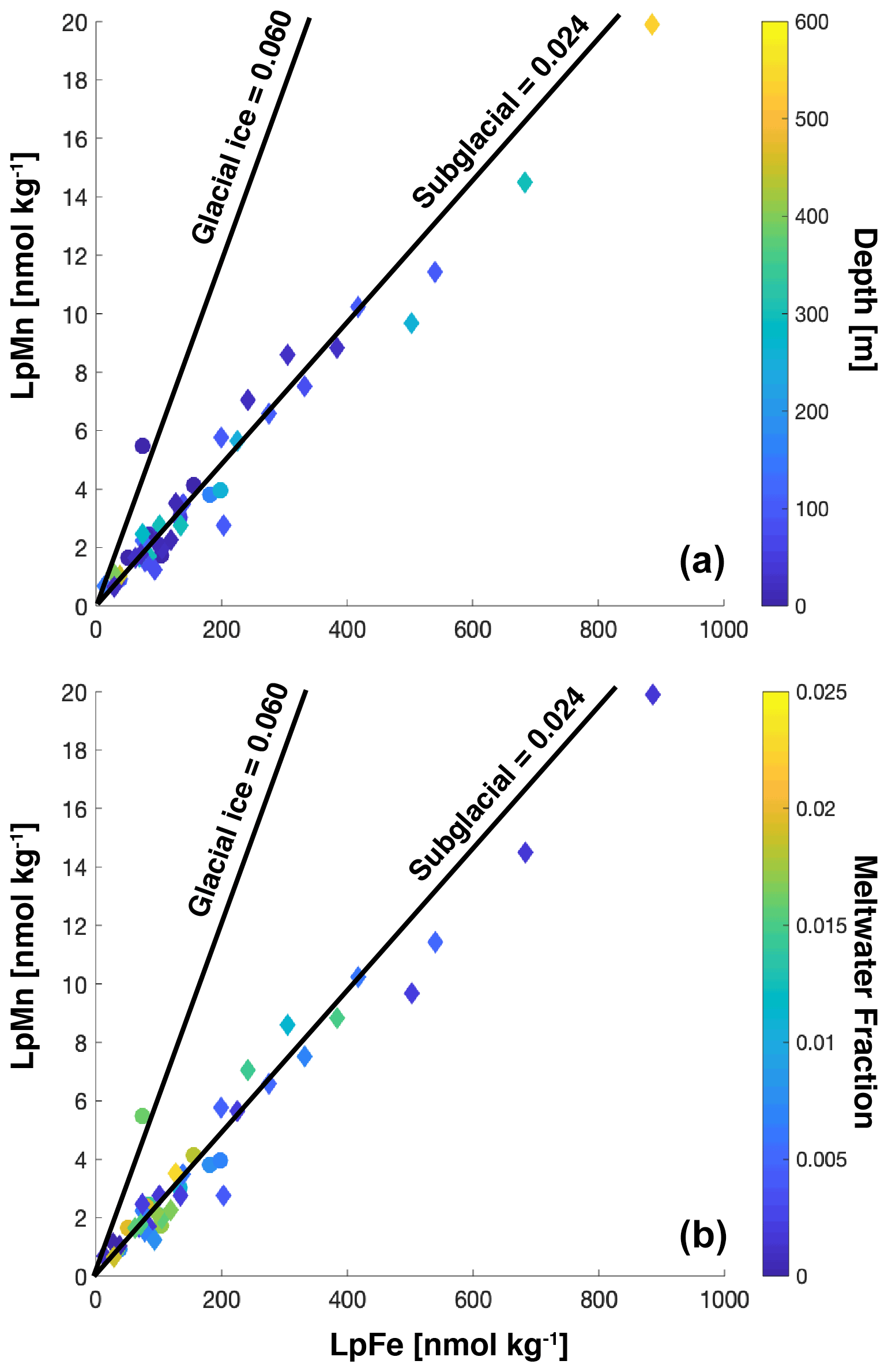
Figure 8Labile particulate Fe and Mn plotted for water column samples. The color bar shows the influence of depth (a) or meltwater fraction (b). For both panels, the December 2015 cruise is indicated by filled circles, and the April 2016 cruise is indicated by filled diamonds. The lines indicate the average ratio of Mn : Fe determined from candidate sources.
4.5 Organic speciation of dissolved Fe
It has been hypothesized that excess ligands (eL = [Lt] − [dFe]) increase the solubility of particulate Fe phases (Thuróczy et al., 2011; Gledhill and Buck, 2012; Wagener et al., 2012; Tagliabue et al., 2019). The persistence of exchangeable pools of dFe would therefore be controlled primarily by particle assemblage and organic ligand complements, where pFe dominates total Fe speciation. We observe consistency between late spring and fall in the relative contribution of dFe to total Fe (4 %–5 % of LpFe, respectively), implying dFe is controlled by scaling closely to LpFe (Fig. 5g, h) since both pools have large interseason differences. An increase in eL between seasons is observed (average 2.1 ± 1.3 nM late spring n=9, 6.0 ± 3.2 nM fall n=12). The ligands are likely produced during microbial high-affinity uptake or remineralization processes following the termination of a bloom (Gledhill and Buck, 2012; Hogle et al., 2016). The only subsurface sample to contain strong Fe-binding ligands is the deep inner basin adjacent to Bagshawe Glacier (IBA), possibly indicating these ligands have a sedimentary source. It appears, based on these results, ligands in Andvord Bay have the capacity to complex additional Fe input, as well as prevent significant loss due to scavenging (Thuróczy et al., 2012). The nature of these ligands, taken together with the low concentration of dFe and abundance of LpFe within the plume, leads us to speculate that Fe minerals are the target for ligand-mediated mineral dissolution and perhaps microbial uptake, previously hypothesized to occur in deep-sea hydrothermal vent plumes (Li et al., 2014). In the fall, despite a greater eL, a lower average conditional stability constant of the ligand pool results in lower complexation capacity and inferred ability to compete with particle binding sites (Ardiningsih et al., 2021). However, the ratio of dFe to LpFe does not reflect a greater enrichment of particles.
While we observe a seasonal increase in the excess ligand concentration, there is no significant change in the ratio of Lt : dFe (late spring 1.8 ± 0.5, fall 2.0 ± 0.7). In the Amundsen sector, Thuróczy et al. (2012) found waters heavily influenced by the Pine Island Glacier to have Lt : dFe ratios < 2.5 throughout the water column, with relatively weaker ligands compared with those found in the highly productive surface waters of the polynya. These findings are similar to an Arctic study, where Ardiningsih et al. (2021) detected weaker ligands close to the 79 N Glacier terminus along the northeast Greenland shelf compared to the adjacent open ocean. We too identify weaker Fe-binding ligands associated with the glaciers, and only at MB and Sill 3 did we observe elevated Lt : dFe (3.13 and 2.99, respectively, in the fall). It is possible that sea ice released strong Fe-binding ligands in Andvord that remained in the surface until sampling in the late spring (Lannuzel et al., 2015). The presence of strong excess Fe-binding ligands at IBA and S3 during the bloom onset also corresponds to elevated NO : dFe (data not shown) above the threshold for potential Fe limitation of coastal diatoms in the California Current region (10–12 µmol nmol−1; King and Barbeau, 2011). The presence of strong Fe-binding ligands might suggest an active microbial strategy in this coastal region to sequester additional Fe from particulate phases during the bloom initiation.
The intense seasonality in primary production and the presence of an undersaturated ligand pool could further increase the bioavailability of particles for downstream communities, where particles within the water column are rare. We calculated the capacity for the free Fe-binding ligands to bind Fe ( (eL⋅K)). Calculations of are included for each sample in Table 2 as well as the inter-seasonal percent change in Fe′ for reoccupied stations (). We find the increased between late spring and fall at IBA and Sill 4, while a decrease was found at the IBB, Sill 3, and Gerlache Strait stations. While all reoccupied stations show an increase in the Fe′ concentration (), the percent change is greatest where decreased in the fall. Thus, the seasonal increase in Fe′ reflects the increase in dFe concentrations as well as lower complexation coefficient of weaker Fe–ligand complexes, which contribute most to dFe speciation in the fall and are associated with surface waters adjacent to glaciers.
These first results of organic speciation of dFe in an Antarctic fjord highlight the importance of seasonal ligand sources in establishing the solubility of new Fe entering the coastal ocean. Accurate ligand pools are not currently represented within SO biogeochemical models (Death et al., 2014; Oliver et al., 2019; Person et al., 2019; St-Laurent et al., 2019). During the bloom initiation, overall ligand strengths are higher than in the fall; however, concentrations of ligands increase following the bloom. Concurrently, dFe concentrations increase and do not saturate the ligands to the same extent as in late spring. This is due to a greater relative increase in ligand concentrations compared to dFe. Ligand-mediated complexation has the potential to greatly expand the spatial extent over which solubilization of particulate Fe occurs and could be critical for sustaining productivity over a larger geographical region (Lippiatt et al., 2010; Ardiningsih et al., 2021). Thus, the size, sinking rate, and composition of particles is critical to their lateral transport and reactivity over time with excess ligands. Our understanding of how cryospheric Fe is transformed after entering the coastal ocean is an important step towards understanding its impact on marine productivity and global biogeochemical cycles of the macronutrients. For the marine Fe cycle, these geochemical transformations control the bioavailability of Fe, while vertical advection and mixing supply this critical micronutrient to the surface ocean and the euphotic zone.
4.6 Using dye experiments to explore Fe sources and export
Rapid communication between the surface and subsurface water masses occurs during katabatic wind events. The large magnitude of vertical shear initializes an upwelling cell close to the inner basins of the fjord. Using an idealized model of a fjord, Lundesgaard et al. (2018) found that katabatic winds can laterally export the surface layer, depending on wind velocity, elapsed time of the event, and whether the wind is along-fjord versus off-axis. Within this idealized model of the fjord, the forcing event leads to outcropping of deeper isohalines (up to 0.3 PSU greater) at the surface along the northern flank of the fjord, corresponding to upwelling (see Fig. 11 in Lundesgaard et al., 2019). Wind-induced overturning circulation, along with deepening of the mixed layer by up to 25 m, would increase surface dFe concentrations at Sill 3. These general model results showed that wind forcing caused water at depths of 50–150 m to upwell rapidly (within 24 h) near the glacier termini. This is an important consequence explored further in the highly resolved model representation of the study region by Hahn-Woernle et al. (2020).
The results of the dye experiments allow for the determination of fluxes, either prescribed (in the case of glacial meltwater) or as a result of wind forcing. St. Laurent et al. (2017) applied similar methods in the Amundsen Sea with explicit coupling of sea ice–ice sheet–ocean interactions (St-Laurent et al., 2017). In a more rigorous biogeochemical model, which included ocean interactions with both sea ice and ice shelves, as well as parameterized Fe reactions, the productive waters in the Amundsen Sea Polynya were supplied by an advected source of dFe from the “meltwater pump” and coastal currents, but this model lacked explicit contributions of subglacial Fe (St-Laurent et al., 2019). These prior modeling results highlight the importance of lateral exchange of surface water masses, providing the impetus to investigate the export of the surface water out of the fjord mouth as explored in the following section.
4.6.1 Surface meltwater Fe sources and export
Given that the MWf varied from 1 %–2.5 % within Andvord Bay during the time of sampling, it is expected that the input of glacial meltwater throughout the melt season would supply some dFe to the surface. We extracted vertical profiles of MWf from the model at Sill 3 and Gerlache Strait stations and found that glacial meltwater originating from Bagshawe and Moser glaciers reaches maximum concentration during the summer bloom (late January 2016) and is relatively constrained to the upper 25 m (Fig. S7b). In early February, when the bloom was terminated, glacial meltwater concentrations in the fjord decreased due to a weakening meltwater input and lateral dispersal. The weakening input is designed to reflect the seasonal cycle of ice melting. Ocean circulation dispersed the meltwater into the Gerlache Strait, as shown by a progressive increase in meltwater in the upper water column throughout the melt season (Fig. S7a). If the volume flux of meltwater input is indeed correlated to the seasonal air temperature cycle, as it is parameterized in the model, the results in Fig. 3 would reaffirm that meltwater is an important control on the accumulation of phytoplankton biomass within Andvord Bay (Pan et al., 2020).
The effect of the wind in driving vertical fluxes will vary with wind direction and location within the fjord. The vertical velocity is analyzed for the observation site at Sill 3 and in front of Bagshawe Glacier (IBA). The latter site is an example location for which katabatic winds are expected to lead to intensified upwelling and is also the location of the subsurface and deep dye experiments. Figure 9a and b depict the relationship between the katabatic wind events and vertical velocities at 20 m: landward-blowing wind generally leads to downwelling, while seaward-blowing katabatic wind leads to upwelling. Based on observations of dFe from the late spring prior to a wind event that started on December 11 ([dFe] at 20 m: 1.97 nM at S3, 2.01 nM at IBA), and the modeled maximum vertical velocities during the wind event (2.09 × 10⁻⁵ m s−1 at S3, 5.08 × 10⁻⁵ m s−1 at IBA), we computed the upwelling flux of dFe into the surface (20 m) at Sill 3 and IBA to be 3.54 and 8.81 µmol m−2 d−1, respectively. These results shed light on the spatial heterogeneity of upwelling conditions within the fjord. Model results for Sill 3 are supported by late spring observations of elevated dFe and low meltwater fraction at this station (Fig. 3). This is also corroborated by increases in surface dFe concentrations observed during repeat occupations of Sill 3 station before (3.19 ± 1.53 nM dFe) and after the wind event (3.94 ± 1.92 nM dFe). We argue that these punctuated periods of upwelling could be a substantial source of dFe to surface waters in Andvord Bay. Further, this supply, together with the flux of glacial meltwater, provides dFe to fuel phytoplankton community growth.
The efficiency with which wind events export the fjord surface water is explored in the glacial meltwater dye experiment. To account for the changing amount of meltwater in the fjord, export across the fjord mouth in Fig. 9c is given as the percentage of the total amount of dye present within the fjord to resolve the effect of katabatic winds on dispersal dynamics of Fe-rich sources. The meltwater dye experiences up to a 28-fold increased export into the Gerlache Strait during periods of strong along-fjord wind, primarily through the surface. To analyze the correlation between along-fjord wind velocity and the relative meltwater export, we first apply a 24 h Gaussian filter to the relative export of glacial meltwater (Fig. 9), to exclude tidal signals. Applying the same filter to the wind time series, we find the wind and export data are positively correlated (r = 0.628). The correlation between export and along-fjord winds supports the results by Lundesgaard et al. (2019), who found that katabatic winds control the export of fjord water. This has important implications for the dispersal of Fe-rich waters downstream, which eventually mix with Fe-poor waters located on the continental shelf (Annett et al., 2017).
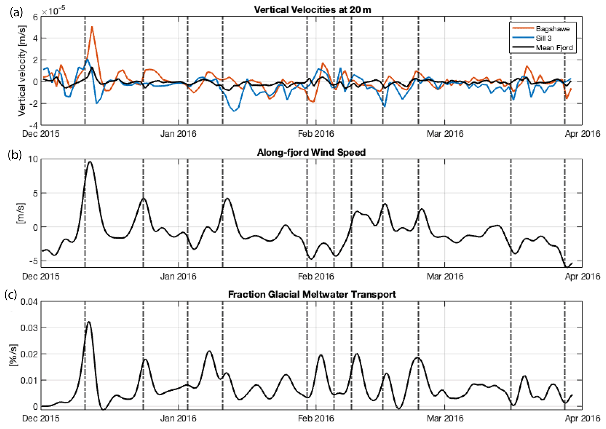
Figure 9(a) Modeled vertical velocities at 20 m for the following locations: Bagshawe Glacier (IBA), Sill 3, and the fjord region average. The 24 h Gaussian filter applied to time series of along-fjord wind velocity (b) and relative meltwater export out of the fjord (c). Wind events exceeding an absolute velocity of 8 m s−1 are indicated by vertical dashed lines. Wind speed data are based on bias-corrected RACMO model output for the center of the fjord, used to force the ROMS model. The transport of meltwater dye is shown relative to the total amount of meltwater dye within Andvord Bay to focus on the physical dynamics and not the changes in volume of dye present in the fjord.
4.6.2 Subsurface and deep sources supplying Fe to export
As discussed in the previous section, periods of vertical mixing due to overturning circulation and mixed layer deepening are shown to occur during katabatic wind events (Lundesgaard et al., 2019, 2020). This could be an important mechanism for supplying additional dFe to the fjord surface from the subglacial plume. We examine this possibility here using the subsurface and deep dye tracers. Prior to the wind event on 11 December, the subsurface dye increases gradually in the upper 20 m (Fig. S6b). With the onset of the wind event, the vertical transport of the subsurface dye into the upper 20 m intensifies and reaches a maximum of 32.7 × 10³ m3 d−1. In comparison, the deep dye does not enter the upper 20 m prior to the wind event, and its maximum vertical transport is only 4.2 × 10³ m3 d−1. It follows that katabatic wind events increase mixing in front of Bagshawe Glacier and have a particularly strong effect on water masses at intermediate depth. Assuming a mean concentration of 8.75 nM dFe for the subsurface plume (Table 1) and 8.68 nM dFe for deep (∼ 300 m) IBA waters in the late spring, these periods of vertical mixing correspond to dFe fluxes of up to 2.81 nmol dFe m−2 d−1 and 0.36 nmol m−2 d−1 (3.17 nmol m−2 d−1 combined) based on the subsurface dye and deep dye, respectively. Following the katabatic wind event, which lasted approximately 11 d, model results show that 36 % of the subsurface dye has shoaled above 75 m, with 10 % of dye found within the surface layer (< 20 m, Fig. S6b). Of the deep water dye, less than 1 % is found within the surface layer. The behavior of the deep water masses suggests an insignificant contribution of deep water masses to the surface hydrography and thus to surface dFe inventory. The vertical fluxes estimated in this section are interpreted as a lower bound for the contribution of the subsurface plume, since the modeled subglacial plume is a fixed volume, when in reality, subglacial meltwater might be supplied continually throughout the melt season. Compared to the flux of surface glacial meltwater input, and the flux due to subsurface and deep water mixing, the upwelling flux generated by wind events is the largest by an order of magnitude.
The quicker export of the subsurface dye, relative to the deep dye, and therefore the low surface dye concentration, is mainly due to its proximity to the ocean surface (Fig. S5b). The upper water column is controlled by katabatic winds, which exports the surface layer out of the fjord mouth. In contrast, the deep dye is exported more slowly and is more continuously released to Gerlache Strait (Fig. S5c). These modeling results provide evidence for the flushing of fjord water to the Gerlache Strait, which coincides with periods of intensified winds. Thus, katabatic winds are important both for replenishing the surface Fe concentrations from the subglacial plume and for exporting Fe-rich surface waters. It is reasonable to assume that in the absence of a strengthened buoyancy-driven overturning circulation, sources from fjord sediments are negligible in supplying the surface with dFe in Andvord Bay.
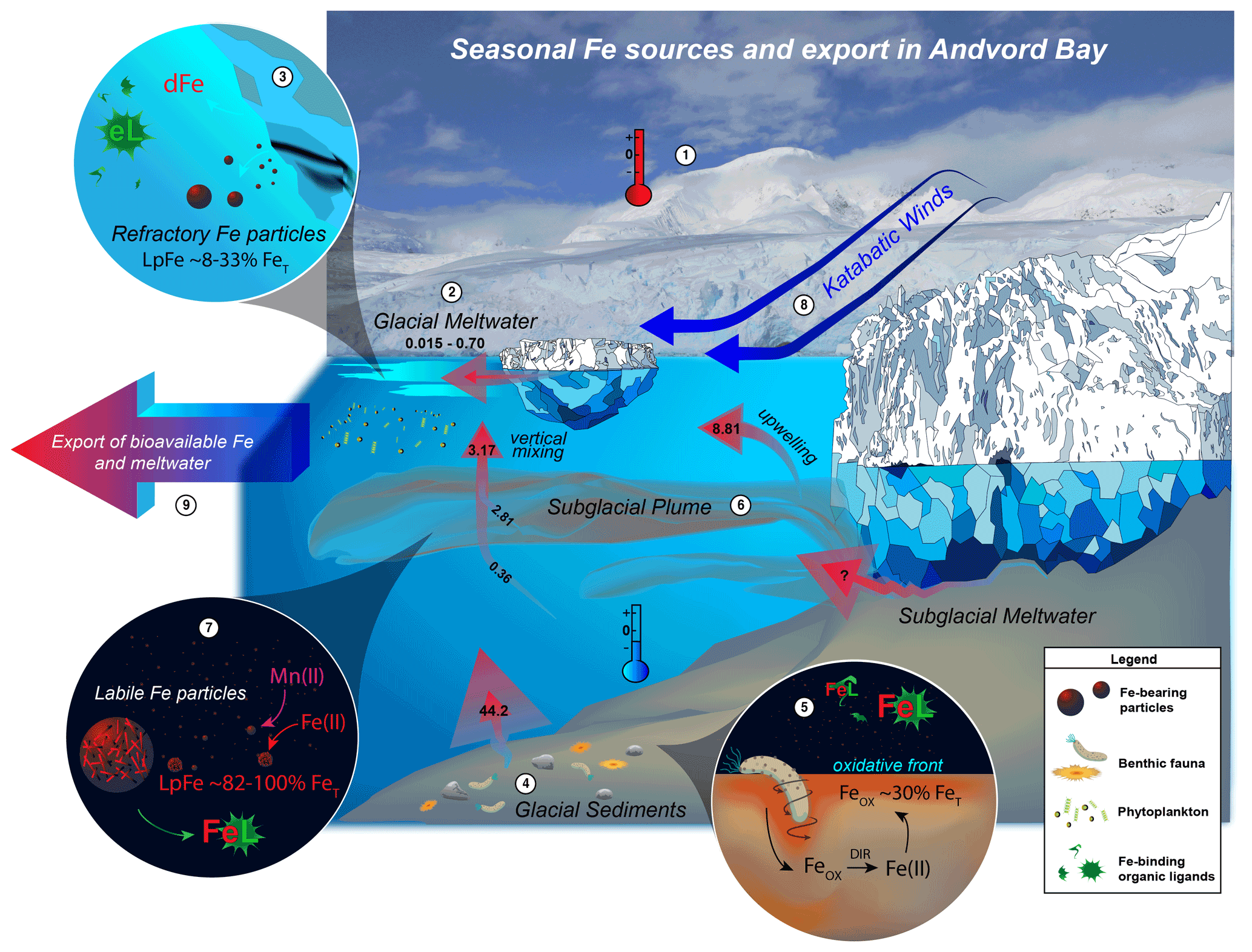
Figure 10Conceptual diagram showing the important seasonal sources of new Fe during the growth and melt season. The red arrows indicate the major fluxes (in µM m−2 d−1), with the size ranges showing the uncertainty in the measurement – some fluxes are difficult to quantify. These fluxes also vary from season to season and from location to location and may even be going through long-term changes due to human influences, such as climate change, though this is not shown here. The small arrows show internal transformations of Fe, which play an important role in the supply of Fe to phytoplankton. See text for a description of important processes highlighted by circled numbers.
4.7 Wind driven meltwater export from WAP fjords
Given that the west Antarctic Peninsula hosts the greatest number of glaciomarine fjords on the continent, and multiple katabatic wind events occur throughout the year, wind events can play a crucial role in the export of Fe and Mn to the larger shelf water region. The modeled export of meltwater integrated over the week after the wind event on December 11 is 38 × 107 m3, which is about 43 % of the meltwater input during the same time. For comparison, during the following week, with relatively calm wind conditions, only 20 % of the meltwater input is exported. We estimate the Fe export to be 272 mol dFe per week and 245 mol dMn per week for this event. However, the warming climate may lessen the likelihood for pulsed export of meltwater-derived Fe by intensifying coastal currents due to declines in sea ice (Moffat et al., 2008) and reduced surface cooling, decreasing the velocity and frequency of katabatic winds over the west Antarctic Ice Sheet (Bintanja et al., 2014).
The large variability in inferred dFe content of glacial meltwaters along the WAP (Annett et al., 2017) means that supply likely depends on fjord-specific processes and future changes in ice volume. Advected sources of dFe remain the largest contribution (∼ 50 %) to the inventory on the productive continental shelves (De Jong et al., 2015), while reducing marine sediments are thought to be the main source of dMn (Annett et al., 2015; Sherrell et al., 2015, 2018). Therefore, we believe that a latitudinal assessment of WAP fjords could begin to address variable responses to ocean and atmospheric forcing in these productive ecosystems. Indeed, less than 160 km south of Andvord Bay, observations of warm modified UCDW intrusions and an invigorated “meltwater pump” present an alternative mechanism for sustaining local primary production in Barilari Bay, a glaciomarine fjord (Cape et al., 2019).
The scope of our results should be highlighted. If we assume Andvord Bay is representative of a typical cold-water fjord, and similarly, Barilari Bay is representative of a warm-water fjord (6 % MWf at surface; Cape et al., 2019), then we can estimate the glacial meltwater export resulting from a single wind event for the entire western coast of the WAP (see Supplement). A total of 3.6 × 10¹⁰ m3 (36 km3) of surface glacial meltwater is exported seaward, which corresponds to 2.0 × 10⁶ mol dFe and 1.8 × 10⁶ mol dMn. Thus, katabatic winds are highly efficient at delivering surface meltwater produced near the coast to the continental shelves and Antarctic Circumpolar Current (ACC), where Fe and Mn limit and co-limit primary production (Browning et al., 2021). However, this volume of surface meltwater exported per year from WAP fjords is small compared to the total basal meltwater production rate due to warm ocean temperatures for the largest ice shelves in Antarctica. Using highly accurate remote sensing topographic measurements, Adusumilli et al. (2020) found that the major Antarctic ice sheets have a steady-state meltwater production value of 1100 ± 60 km3 yr−1. In a different modeling study, it was estimated that 300–800 km3 yr−1 meltwater enters the SO accounting for observed trends in SO sea surface temperature, sea ice expansion, and sea surface height (Rye et al., 2020). The “effective” fluxes of Fe and Mn may be lower than what was calculated here because of the non-conservative behavior of these elements during their lateral advection to the shelf. It should be noted that the WAP feeds most directly into the Antarctic Circumpolar Current (ACC), which advects modified coastal waters downstream to the productive Scotia Sea region, potentially magnifying the ecological impact of WAP fjord meltwater production.
We have argued that, for glaciers terminating in cold-water fjords with a resultant absence of buoyancy-driven upwelling, the interaction of the ice sheet, atmosphere, and surface ocean is important for resupplying the surface waters with Fe throughout the summer season. Using a high-resolution ROMS model of the study region, we showed katabatic wind events result in pulsed export of the surface layer to the adjacent shelf water, while upwelling and vertical mixing entrains subglacial plume water in the inner fjord. Observed surface concentrations of dFe in fall lend support to these modeled dynamics since elevated concentrations of dFe and meltwater are found within the inner fjord and at Sill 3 (see Fig. 3). At both fjord locations, upwelling of subsurface water masses occurs, potentially entraining subglacial plume water. We summarize the findings of this study in a conceptual diagram showing important seasonal sources of Fe during the growth and melt season (Fig. 10). We highlight important processes in the diagram using circled number notation. We found ocean temperatures are cold ① and do not melt the fronts of glaciers, but warm summer atmospheric temperatures contribute to the surface melting of glacial ice ②. Variability in dissolved and particulate Fe concentrations in glacial ice imposes large uncertainties in the calculated Fe flux associated with melting. Iron occurs in glacial ice predominantly in the form of refractory Fe-bearing mineral particles ③. Only a small fraction of Fe from these particles may be stabilized by excess organic ligands. Another Fe source is fjord sediments ④, though there is considerable uncertainty shown in the magnitude of this flux because evidence indicates that a significant fraction of porewater Fe rapidly precipitates at the oxidative front, forming a rich surface layer of Fe oxyhydroxides at the sediment surface ⑤. Intense bioturbation of fjord sediments mixes the surface sediments downwards, fueling redox processes in deeper sediment layers. The dFe that escapes this sink enriches deep waters within the fjord basins. Small amounts of subglacial meltwater discharge enter the ocean and form turbid buoyant subsurface plumes ⑥. Within the plumes, speciation is dominated by high concentrations of labile authigenic Fe-bearing particles that can be solubilized by Fe-binding organic ligands ⑦. Seaward-blowing katabatic winds ⑧ occur episodically and cause upwelling and vertical mixing, supplying additional Fe to the surface phytoplankton assemblage. These intense energetic periods facilitate the dispersion and export of surface Fe, Mn, and meltwater away from the fjord where it is advected downstream in the Gerlache Strait and into the Bransfield Strait ⑨.
In Andvord Bay, primary production will be sensitive to future changes in subglacial discharge as Antarctic glaciers continue to melt in response to oceanic and atmospheric warming (Smith et al., 2020). In the short term, increased Fe and Mn supply may increase primary production. Conversely, in the long term, increased meltwater discharge will generate a greater flux of sediment to the fjord (Brinkerhoff et al., 2017), reducing light availability for primary producers, while stratifying the upper water column and preventing nutrient replenishment (Hopwood et al., 2018). A key question outside the scope of this research is how the quantity and quality of Fe-binding ligands will change in the future. To a first approximation, decreases in the magnitude of local phytoplankton blooms and associated ligand sources is expected to reduce efficacy of solubilization of particulate Fe and natural fertilization downstream resulting from this fjord. This climatic trend is not yet realized within Andvord Bay (Eidam et al., 2019) but is expected to decrease dFe export through increased scavenging and sedimentation, further resembling high-Arctic and temperate fjords (Hopwood et al., 2016).
All CTD data from this study are available at the US Antarctic Program (USAP) Data Center: https://doi.org/10.15784/601158 (Vernet et al., 2019).
The supplement related to this article is available online at: https://doi.org/10.5194/bg-18-6349-2021-supplement.
KOF designed the study, conducted the analyses, and led the writing of the manuscript. LHW performed numerical dye simulations. RMS, VJR, and KB assisted in the preparation of multi-elemental analyses. DB provided data for sediment core analyses. LHW, RMS, DB, MV, and KAB were involved in discussing the results and their implications and contributed to the drafting of the manuscript.
The authors declare that they have no conflict of interest.
Publisher’s note: Copernicus Publications remains neutral with regard to jurisdictional claims in published maps and institutional affiliations.
The authors would like to thank all participating principal investigators and their affiliates during the NSF FjordEco project. Lauren Manck (University of Montana) assisted with sampling efforts during NBP1603. We would like to thank the captain and crew of R/V Laurence M. Gould and RVIB Nathaniel B. Palmer and United States Antarctic Program contractors. We also thank Brian Powell (University of Hawai'i, Manoa) for helpful comments and for providing resources for the modeling effort. We would also like to thank the two anonymous reviewers for their attention to detail. Their efforts have greatly improved this paper.
This research has been supported by the National Science Foundation (grant no. PLR-1443705). Funding for speciation work was funded through an NSF grant (NSF OCE-1558841). Kiefer Forsch was supported by an NSF GRF (NSF 15-597).
This paper was edited by Jack Middelburg and reviewed by Rob Middag and one anonymous referee.
Alderkamp, A. C., Mills, M. M., van Dijken, G. L., Laan, P., Thuróczy, C. E., Gerringa, L. J. A., de Baar, H. J. W., Payne, C. D., Visser, R. J. W., Buma, A. G. J., and Arrigo, K. R.: Iron from melting glaciers fuels phytoplankton blooms in the Amundsen Sea (Southern Ocean): Phytoplankton characteristics and productivity, Deep-Sea Res. Pt. II, 71–76, 32–48, https://doi.org/10.1016/j.dsr2.2012.03.005, 2012.
Annett, A. L., Skiba, M., Henley, S. F., Venables, H. J., Meredith, M. P., Statham, P. J., and Ganeshram, R. S.: Comparative roles of upwelling and glacial iron sources in Ryder Bay, coastal western Antarctic Peninsula, Mar. Chem., 76, 21–33, https://doi.org/10.1016/j.marchem.2015.06.017, 2015.
Annett, A. L., Fitzsimmons, J. N., Séguret, M. J. M., Lagerström, M., Meredith, M. P., Schofield, O., and Sherrell, R. M.: Controls on dissolved and particulate iron distributions in surface waters of the Western Antarctic Peninsula shelf, Mar. Chem., 196, 81–97, https://doi.org/10.1016/j.marchem.2017.06.004, 2017.
Ardelan, M. V, Holm-Hansen, O., Hewes, C. D., Reiss, C. S., Silva, N. S., Dulaiova, H., Steinnes, E., and Sakshaug, E.: Natural iron enrichment around the Antarctic Peninsula in the Southern Ocean, Biogeosciences, 7, 11–25, https://doi.org/10.5194/bg-7-11-2010, 2010.
Ardiningsih, I., Seyitmuhammedov, K., Sander, S. G., Stirling, C. H., Reichart, G.-J., Arrigo, K. R., Gerringa, L. J. A., and Middag, R.: Fe-binding organic ligands in coastal and frontal regions of the western Antarctic Peninsula, Biogeosciences, 18, 4587–4601, https://doi.org/10.5194/bg-18-4587-2021, 2021.
Armstrong, P. B., Lyons, W. B., and Gaudette, H. E.: Application of Formaldoxime Colorimetric Method for the Determination of Manganese in the Pore Water of Anoxic Estuarine Sediments, Estuaries, 2, 198–201, https://doi.org/10.2307/1351736, 1979.
Bintanja, R., Severijns, C., Haarsma, R., and Hazeleger, W.: The future of Antarctica's surface winds simulated by a high-resolution global climate model: 1. Model description and validation, J. Geophys. Res.-Atmos., 119, 7136–7159, https://doi.org/10.1002/2013JD020847, 2014.
Boudreau, B. P.: The diffusive tortuosity of fine-grained unlithified sediments, Geochim. Cosmochim. Ac., 60, 3139–3142, https://doi.org/10.1016/0016-7037(96)00158-5, 1996.
Bown, J., van Haren, H., Meredith, M. P., Venables, H. J., Laan, P., Brearley, J. A., and de Baar, H. J. W.: Evidences of strong sources of DFe and DMn in Ryder Bay, Western Antarctic Peninsula, Philos. Trans. A, 376, 20170172, https://doi.org/10.1098/rsta.2017.0172, 2018.
Boyd, P. W., Claustre, H., Levy, M., Siegel, D. A., and Weber, T.: Multi-faceted particle pumps drive carbon sequestration in the ocean, Nature, 568, 327–335, https://doi.org/10.1038/s41586-019-1098-2, 2019.
Boyle, E. A., Edmond, J. M., and Sholkovitz, E. R.: The mechanism of iron removal in estuaries, Geochim. Cosmochim. Ac., 41, 1313–1324, https://doi.org/10.1016/0016-7037(77)90075-8, 1977.
Brendel, P. J. and Luther, G. W.: Development of a Gold Amalgam Voltammetric Microelectrode for the Determination of Dissolved Fe, Mn, O2, and S(-II) in Porewaters of Marine and Freshwater Sediments, Environ. Sci. Technol., 29, 751–761, https://doi.org/10.1021/es00003a024, 1995.
Brinkerhoff, D., Truffer, M., and Aschwanden, A.: Sediment transport drives tidewater glacier periodicity, Nat. Commun., 8, 90, https://doi.org/10.1038/s41467-017-00095-5, 2017.
Browning, T. J., Achterberg, E. P., Engel, A., and Mawji, E.: Manganese co-limitation of phytoplankton growth and major nutrient drawdown in the Southern Ocean, Nat. Commun., 12, 884, https://doi.org/10.1038/s41467-021-21122-6, 2021.
Buck, K. N., Sohst, B., and Sedwick, P. N.: The organic complexation of dissolved iron along the U.S. GEOTRACES (GA03) North Atlantic Section, Deep-Sea Res. Pt. II, 116, 152–165, https://doi.org/10.1016/j.dsr2.2014.11.016, 2015.
Buck, K. N., Sedwick, P. N., Sohst, B., and Carlson, C. A.: Organic complexation of iron in the eastern tropical South Pacific: Results from US GEOTRACES Eastern Pacific Zonal Transect (GEOTRACES cruise GP16), Mar. Chem., 201, 229–241, https://doi.org/10.1016/j.marchem.2017.11.007, 2018.
Burdige, D. J. and Komada, T.: Iron redox cycling, sediment resuspension and the role of sediments in low oxygen environments as sources of iron to the water column, Mar. Chem., 223, 103793, https://doi.org/10.1016/j.marchem.2020.103793, 2020.
Cape, M. R., Vernet, M., Pettit, E. C., Wellner, J., Truffer, M., Akie, G., Domack, E., Leventer, A., Smith, C. R., and Huber, B. A.: Circumpolar Deep Water Impacts Glacial Meltwater Export and Coastal Biogeochemical Cycling Along the West Antarctic Peninsula, Front. Mar. Sci., 6, 144 pp., 2019.
Cook, A. J., Holland, P. R., Meredith, M. P., Murray, T., Luckman, A., and Vaughan, D. G.: Ocean forcing of glacier retreat in the western Antarctic Peninsula, Science, 353, 283–286, https://doi.org/10.1126/science.aae0017, 2016.
Cowan, E. A. and Powell, R. D.: Suspended sediment transport and deposition of cyclically interlaminated sediment in a temperate glacial fjord, Alaska, USA, Geol. Soc. Lond. Spec. Publ., 53, 75–89, https://doi.org/10.1144/GSL.SP.1990.053.01.04, 1990.
Cutter, G. A. and Bruland, K. W.: Rapid and noncontaminating sampling system for trace elements in global ocean surveys, Limnol. Oceanogr. Method., 10, 425–436, https://doi.org/10.4319/lom.2012.10.425, 2012.
Dale, A. W., Nickelsen, L., Scholz, F., Hensen, C., Oschlies, A., and Wallmann, K.: A revised global estimate of dissolved iron fluxes from marine sediments, Global Biogeochem. Cy., 29, 691–707, https://doi.org/10.1002/2014GB005017, 2015.
Death, R., Wadham, J. L., Monteiro, F., Le Brocq, A. M., Tranter, M., Ridgwell, A., Dutkiewicz, S., and Raiswell, R.: Antarctic ice sheet fertilises the Southern Ocean, Biogeosciences, 11, 2635–2643, https://doi.org/10.5194/bg-11-2635-2014, 2014.
De Jong, J. T. M., Stammerjohn, S. E., Ackley, S. F., Tison, J.-L., Mattielli, N., and Schoemann, V.: Sources and fluxes of dissolved iron in the Bellingshausen Sea (West Antarctica): The importance of sea ice, icebergs and the continental margin, Mar. Chem., 177, 518–535, https://doi.org/10.1016/j.marchem.2015.08.004, 2015.
Dierssen, H. M., Smith, R. C., and Vernet, M.: Glacial meltwater dynamics in coastal waters west of the Antarctic peninsula, P. Natl. Acad. Sci. USA, 99, 1790–1795, https://doi.org/10.1073/pnas.032206999, 2002.
Domack, E. W. and Ishman, S.: Oceanographic and physiographic controls on modern sedimentation within Antarctic fjords, Geol. Soc. Am. Bull., 105, 1175–1189, 1993.
Domack, E. W. and Williams, C. R.: Fine Structure and Suspended Sediment Transport in Three Antarctic Fjords [Internet], Contributions to Antarctic Research I, Antarctic Research Series, 71–89, available at: https://doi.org/10.1029/AR050p0071, 1990.
Egbert, G. D. and Erofeeva, S. Y.: Efficient Inverse Modeling of Barotropic Ocean Tides, J. Atmos. Ocean. Technol., 19, 183–204, https://doi.org/10.1175/1520-0426(2002)019<0183:EIMOBO>2.0.CO;2, 2002.
Eidam, E. F., Nittrouer, C. A., Lundesgaard, Homolka, K. K., and Smith, C. R.: Variability of Sediment Accumulation Rates in an Antarctic Fjord, Geophys. Res. Lett., 46, 13271–13280, https://doi.org/10.1029/2019GL084499, 2019.
Ekern, L.: Assessing Primary Production via nutrient deficits in Andvord Bay, Antarctica 2015–2016, University of California, San Diego, 2017.
Fitzsimmons, J. N., Bundy, R. M., Al-Subiai, S. N., Barbeau, K. A., and Boyle, E. A.: The composition of dissolved iron in the dusty surface ocean: An exploration using size-fractionated iron-binding ligands, Mar. Chem., 173, 125–135, https://doi.org/10.1016/j.marchem.2014.09.002, 2015.
Fitzsimmons, J. N., John, S. G., Marsay, C. M., Hoffman, C. L., Nicholas, S. L., Toner, B. M., German, C. R., and Sherrell, R. M.: Iron persistence in a distal hydrothermal plume supported by dissolved–particulate exchange, Nat. Geosci., 10, 195–201, https://doi.org/10.1038/ngeo2900, 2017.
Gerringa, L. J. A., Laan, P., van Dijken, G. L., van Haren, H., De Baar, H. J. W., Arrigo, K. R., and Alderkamp, A. C.: Sources of iron in the Ross Sea polynya in early summer, Mar. Chem., 177, 447–459, 2015.
Gerringa, L. J. A., Gledhill, M., Ardiningsih, I., Muntjewerf, N., and Laglera, L. M.: Comparing CLE-AdCSV applications using SA and TAC to determine the Fe-binding characteristics of model ligands in seawater, Biogeosciences, 18, 5265–5289, https://doi.org/10.5194/bg-18-5265-2021, 2021.
Gledhill, M. and Buck, K. N.: The organic complexation of iron in the marine environment: a review, Front. Microbiol., 3, 69, https://doi.org/10.3389/fmicb.2012.00069, 2012.
Goldberg, T., Archer, C., Vance, D., Thamdrup, B., McAnena, A., and Poulton, S. W.: Controls on Mo isotope fractionations in a Mn-rich anoxic marine sediment, Gullmar Fjord, Sweden, Chem. Geol., 296/297, 73–82, https://doi.org/10.1016/j.chemgeo.2011.12.020, 2012.
Grange, L. J. and Smith, C. R.: Megafaunal communities in rapidly warming fjords along the West Antarctic Peninsula: Hotspots of abundance and beta diversity, PLoS One, 8, 12, https://doi.org/10.1371/journal.pone.0077917, 2013.
Hahn-Woernle, L., Powell, B., Lundesgaard, Ø., and van Wessem, M.: Sensitivity of the summer upper ocean heat content in a Western Antarctic Peninsula fjord, Prog. Oceanogr., 183, 102287, https://doi.org/10.1016/j.pocean.2020.102287, 2020.
Haidvogel, D. B., Arango, H., Budgell, W. P., Cornuelle, B. D., Curchitser, E., Di Lorenzo, E., Fennel, K., Geyer, W. R., Hermann, A. J., Lanerolle, L., Levin, J., McWilliams, J. C., Miller, A. J., Moore, A. M., Powell, T. M., Shchepetkin, A. F., Sherwood, C. R., Signell, R. P., Warner, J. C., and Wilkin, J.: Ocean forecasting in terrain-following coordinates: Formulation and skill assessment of the Regional Ocean Modeling System, J. Comput. Phys., 227, 3595–3624, https://doi.org/10.1016/j.jcp.2007.06.016, 2008.
Halbach, L., Vihtakari, M., Duarte, P., Everett, A., Granskog, M. A., Hop, H., Kauko, H. M., Kristiansen, S., Myhre, P. I., Pavlov, A. K., Pramanik, A., Tatarek, A., Torsvik, T., Wiktor, J. M., Wold, A., Wulff, A., Steen, H., and Assmy, P.: Tidewater Glaciers and Bedrock Characteristics Control the Phytoplankton Growth Environment in a Fjord in the Arctic , Front. Mar. Sci., 6, 254, https://doi.org/10.3389/fmars.2019.00254, 2019.
Hatta, M., Measures, C. I., Selph, K. E., Zhou, M., and Hiscock, W. T.: Iron fluxes from the shelf regions near the South Shetland Islands in the Drake Passage during the austral-winter 2006, Deep-Sea Res. Pt. II, 90, 89–101, https://doi.org/10.1016/j.dsr2.2012.11.003, 2013.
Hawkings, J. R., Wadham, J. L., Tranter, M., Raiswell, R., Benning, L. G., Statham, P. J., Tedstone, A., Nienow, P., Lee, K., and Telling, J.: Ice sheets as a significant source of highly reactive nanoparticulate iron to the oceans., Nat. Commun., 5, 3929, https://doi.org/10.1038/ncomms4929, 2014.
Hawkings, J. R., Hatton, J. E., Hendry, K. R., de Souza, G. F., Wadham, J. L., Ivanovic, R., Kohler, T. J., Stibal, M., Beaton, A., Lamarche-Gagnon, G., Tedstone, A., Hain, M. P., Bagshaw, E., Pike, J., and Tranter, M.: The silicon cycle impacted by past ice sheets, Nat. Commun., 9, 3210, https://doi.org/10.1038/s41467-018-05689-1, 2018.
Hawkings, J. R., Skidmore, M. L., Wadham, J. L., Priscu, J. C., Morton, P. L., Hatton, J. E., Gardner, C. B., Kohler, T. J., Stibal, M., Bagshaw, E. A., Steigmeyer, A., Barker, J., Dore, J. E., Lyons, W. B., Tranter, M., and Spencer, R. G. M.: Enhanced trace element mobilization by Earth's ice sheets, P. Natl. Acad. Sci. USA, 117, 31648–31659, https://doi.org/10.1073/pnas.2014378117, 2020.
Henkel, S., Kasten, S., Hartmann, J. F., Silva-Busso, A., and Staubwasser, M.: Iron cycling and stable Fe isotope fractionation in Antarctic shelf sediments, King George Island, Geochim. Cosmochim. Ac., 237, 320–338, https://doi.org/10.1016/j.gca.2018.06.042, 2018.
Henley, S. F., Cavan, E. L., Fawcett, S. E., Kerr, R., Monteiro, T., Sherrell, R. M., Bowie, A. R., Boyd, P. W., Barnes, D. K. A., Schloss, I. R., Marshall, T., Flynn, R., and Smith, S.: Changing Biogeochemistry of the Southern Ocean and Its Ecosystem Implications, Front. Mar. Sci., 7, 581, https://doi.org/10.3389/fmars.2020.00581, 2020.
Hopwood, M. J., Cantoni, C., Clarke, J. S., Cozzi, S., and Achterberg, E. P.: The heterogeneous nature of Fe delivery from melting icebergs, Geochem. Perspect. Lett., 3, 200–209, https://doi.org/10.7185/geochemlet.1723, 2017.
Hodson, A., Nowak, A., Sabacka, M., Jungblut, A., Navarro, F., Pearce, D., Ávila-Jiménez, M. L., Convey, P., and Vieira, G.: Climatically sensitive transfer of iron to maritime Antarctic ecosystems by surface runoff, Nat. Commun., 8, 14499, https://doi.org/10.1038/ncomms14499, 2017.
Hogle, S. L., Bundy, R. M., Blanton, J. M., Allen, E. E., and Barbeau, K. A.: Copiotrophic marine bacteria are associated with strong iron-binding ligand production during phytoplankton blooms, Limnol. Oceanogr. Lett., 1, 36–43, https://doi.org/10.1002/lol2.10026, 2016.
Holding, J. M., Markager, S., Juul-Pedersen, T., Paulsen, M. L., Møller, E. F., Meire, L., and Sejr, M. K.: Seasonal and spatial patterns of primary production in a high-latitude fjord affected by Greenland Ice Sheet run-off, Biogeosciences, 16, 3777–3792, https://doi.org/10.5194/bg-16-3777-2019, 2019.
Hopwood, M. J., Bacon, S., Arendt, K., Connelly, D. P., and Statham, P. J.: Glacial meltwater from Greenland is not likely to be an important source of Fe to the North Atlantic, Biogeochemistry, 124, 1–11, https://doi.org/10.1007/s10533-015-0091-6, 2015.
Hopwood, M. J., Connelly, D. P., Arendt, K. E., Juul-Pedersen, T., Stinchcombe, M., Meire, L., Esposito, M., and Krishna, R.: Seasonal changes in Fe along a glaciated Greenlandic fjord, Front. Earth Sci. , 4, 1–13, https://doi.org/10.3389/feart.2016.00015, 2016.
Hopwood, M. J., Carroll, D., Höfer, J., Achterberg, E. P., Meire, L., Le Moigne, F. A. C., Bach, L. T., Eich, C., Sutherland, D. A., and González, H. E.: Highly variable iron content modulates iceberg-ocean fertilisation and potential carbon export, Nat. Commun., 10, 5261, https://doi.org/10.1038/s41467-019-13231-0, 2019.
Jack Pan, B., Vernet, M., Reynolds, R. A., and Greg Mitchell, B.: The optical and biological properties of glacial meltwater in an Antarctic fjord, PLoS One, 14, e0211107, https://doi.org/10.1371/journal.pone.0211107, 2019.
Jackson, R. H., Straneo, F., and Sutherland, D. A.: Externally forced fluctuations in ocean temperature at Greenland glaciers in non-summer months, Nat. Geosci., 7, 503–508, https://doi.org/10.1038/ngeo2186, 2014.
Kanna, N., Sugiyama, S., Fukamachi, Y., Nomura, D., and Nishioka, J.: Iron Supply by Subglacial Discharge Into a Fjord Near the Front of a Marine-Terminating Glacier in Northwestern Greenland, Global Biogeochem. Cy., 34, e2020GB006567, https://doi.org/10.1029/2020GB006567, 2020.
King, A. L. and Barbeau, K. A.: Dissolved iron and macronutrient distributions in the southern California Current System, J. Geophys. Res. Ocean., 116, C03018, https://doi.org/10.1029/2010JC006324, 2011.
Komada, T., Burdige, D. J., Magen, C., Li, H.-L., and Chanton, J.: Recycling of Organic Matter in the Sediments of Santa Monica Basin, California Borderland, Aquat. Geochem., 22, 593–618, https://doi.org/10.1007/s10498-016-9308-0, 2016.
Krisch, S., Hopwood, M. J., Schaffer, J., Al-Hashem, A., Höfer, J., Rutgers van der Loeff, M. M., Conway, T. M., Summers, B. A., Lodeiro, P., Ardiningsih, I., Steffens, T., and Achterberg, E. P.: The 79∘N Glacier cavity modulates subglacial iron export to the NE Greenland Shelf, Nat. Commun., 12, 3030, https://doi.org/10.1038/s41467-021-23093-0, 2021.
Kryc, K. A., Murray, R. W., and Murray, D. W.: Al-to-oxide and Ti-to-organic linkages in biogenic sediment: relationships to paleo-export production and bulk Al Ti, Earth Planet. Sc. Lett., 211, 125–141, https://doi.org/10.1016/S0012-821X(03)00136-5, 2003.
Lagerström, M. E., Field, M. P., Séguret, M., Fischer, L., Hann, S., and Sherrell, R. M.: Automated on-line flow-injection ICP-MS determination of trace metals (Mn, Fe, Co, Ni, Cu and Zn) in open ocean seawater: Application to the GEOTRACES program, Mar. Chem., 155, 71–80, https://doi.org/10.1016/j.marchem.2013.06.001, 2013.
Lannuzel, D., Grotti, M., Abelmoschi, M. L., and van der Merwe, P.: Organic ligands control the concentrations of dissolved iron in Antarctic sea ice, Mar. Chem., 174, 120–130, https://doi.org/10.1016/j.marchem.2015.05.005, 2015.
Laufer-Meiser, K., Michaud, A. B., Maisch, M., Byrne, J. M., Kappler, A., Patterson, M. O., Røy, H., and Jørgensen, B. B.: Potentially bioavailable iron produced through benthic cycling in glaciated Arctic fjords of Svalbard, Nat. Commun., 12, 1349, https://doi.org/10.1038/s41467-021-21558-w, 2021.
Li, M., Toner, B. M., Baker, B. J., Breier, J. A., Sheik, C. S., and Dick, G. J.: Microbial iron uptake as a mechanism for dispersing iron from deep-sea hydrothermal vents, Nat. Commun., 5, 3192, https://doi.org/10.1038/ncomms4192, 2014.
Lippiatt, S. M., Lohan, M. C., and Bruland, K. W.: The distribution of reactive iron in northern Gulf of Alaska coastal waters, Mar. Chem., 121, 187–199, https://doi.org/10.1016/j.marchem.2010.04.007, 2010.
Lohan, M. C., Aguilar-Islas, A. M., and Bruland, K. W.: Direct determination of iron in acidified (pH 1.7) seawater samples by flow injection analysis with catalytic spectrophotometric detection: Application and intercomparison, Limnol. Oceanogr. Method., 4, 164–171, https://doi.org/10.4319/lom.2006.4.164, 2006.
Lundesgaard, Ø., Powell, B., Merrifield, M., Hahn-Woernle, L., and Winsor, P.: Response of an antarctic Peninsula fjord to summer Katabatic wind events, J. Phys. Oceanogr., 49, 1485–1502, https://doi.org/10.1175/JPO-D-18-0119.1, 2019.
Lundesgaard, Ø., Winsor, P., Truffer, M., Merrifield, M., Powell, B., Statscewich, H., Eidam, E., and Smith, C. R.: Hydrography and energetics of a cold subpolar fjord: Andvord Bay, western Antarctic Peninsula, Prog. Oceanogr., 181, 102224, https://doi.org/10.1016/j.pocean.2019.102224, 2020.
Luther, G. W., Glazer, B. T., Ma, S., Trouwborst, R. E., Moore, T. S., Metzger, E., Kraiya, C., Waite, T. J., Druschel, G., Sundby, B., Taillefert, M., Nuzzio, D. B., Shank, T. M., Lewis, B. L., and Brendel, P. J.: Use of voltammetric solid-state (micro)electrodes for studying biogeochemical processes: Laboratory measurements to real time measurements with an in situ electrochemical analyzer (ISEA), Mar. Chem., 108, 221–235, https://doi.org/10.1016/j.marchem.2007.03.002, 2008.
Luther III, G. W., Brendel, P. J., Lewis, B. L., Sundby, B., Lefrançois, L., Silverberg, N., and Nuzzio, D. B.: Simultaneous measurement of O2, Mn, Fe, I-, and S(–II) in marine pore waters with a solid-state voltammetric microelectrode, Limnol. Oceanogr., 43, 325–333, https://doi.org/10.4319/lo.1998.43.2.0325, 1998.
Marsay, C. M., Sedwick, P. N., Dinniman, M. S., Barrett, P. M., Mack, S. L., and McGillicuddy, D. J.: Estimating the benthic efflux of dissolved iron on the Ross Sea continental shelf, Geophys. Res. Lett., 41, 7576–7583, https://doi.org/10.1002/2014GL061684, 2014.
Martin, J. H., Gordon, R. M., and Fitzwater, S. E.: Iron in Antarctic waters, Nature, 345, 156–158, https://doi.org/10.1038/345156a0, 1990.
Meire, L., Mortensen, J., Meire, P., Juul-Pedersen, T., Sejr, M. K., Rysgaard, S., Nygaard, R., Huybrechts, P., and Meysman, F. J. R.: Marine-terminating glaciers sustain high productivity in Greenland fjords, Glob. Change Biol., 23, 5344–5357, https://doi.org/10.1111/gcb.13801, 2017.
Meredith, M. P., Stammerjohn, S. E., Venables, H. J., Ducklow, H. W., Martinson, D. G., Iannuzzi, R. A., Leng, M. J., van Wessem, J. M., Reijmer, C. H., and Barrand, N. E.: Changing distributions of sea ice melt and meteoric water west of the Antarctic Peninsula, Deep-Sea Res. Pt. II, 139, 40–57, https://doi.org/10.1016/j.dsr2.2016.04.019, 2017.
Mikucki, J. A., Pearson, A., Johnston, D. T., Turchyn, A. V, Farquhar, J., Schrag, D. P., Anbar, A. D., Priscu, J. C., and Lee, P. A.: A Contemporary Microbially Maintained Subglacial Ferrous “Ocean”, Science, 324, 397–400, https://doi.org/10.1126/science.1167350, 2009.
Moffat, C., Beardsley, R. C., Owens, B., and van Lipzig, N.: A first description of the Antarctic Peninsula Coastal Current, Deep-Sea Res. Pt. II, 55, 277–293, https://doi.org/10.1016/j.dsr2.2007.10.003, 2008.
Mouginot, J., Rignot, E., Bjørk, A. A., van den Broeke, M., Millan, R., Morlighem, M., Noël, B., Scheuchl, B.,, and Wood, M.: Forty-six years of Greenland Ice Sheet mass balance from 1972 to 2018, P. Natl. Acad. Sci. USA, 116, 9239–9244, https://doi.org/10.1073/pnas.1904242116, 2019.
Ng, H. C., Cassarino, L., Pickering, R. A., Woodward, E. M. S., Hammond, S. J., and Hendry, K. R.: Sediment efflux of silicon on the Greenland margin and implications for the marine silicon cycle, Earth Planet. Sc. Lett., 529, 115877, https://doi.org/10.1016/j.epsl.2019.115877, 2020.
Oliver, H., St-Laurent, P., Sherrell, R. M., and Yager, P. L.: Modeling Iron and Light Controls on the Summer Phaeocystis antarctica Bloom in the Amundsen Sea Polynya, Global Biogeochem. Cy., 33, 570–596, https://doi.org/10.1029/2018GB006168, 2019.
Omanović, D., Garnier, C., and Pižeta, I.: ProMCC: An all-in-one tool for trace metal complexation studies, Mar. Chem., 173, 25–39, https://doi.org/10.1016/j.marchem.2014.10.011, 2015.
Pan, B. J., Vernet, M., Manck, L., Forsch, K., Ekern, L., Mascioni, M., Barbeau, K. A., Almandoz, G. O., and Orona, A. J.: Environmental drivers of phytoplankton taxonomic composition in an Antarctic fjord, Prog. Oceanogr., 183, 102295, https://doi.org/10.1016/j.pocean.2020.102295, 2020.
Person, R., Aumont, O., Madec, G., Vancoppenolle, M., Bopp, L., and Merino, N.: Sensitivity of ocean biogeochemistry to the iron supply from the Antarctic Ice Sheet explored with a biogeochemical model, Biogeosciences, 16, 3583–3603, https://doi.org/10.5194/bg-16-3583-2019, 2019.
Poulton, S. W. and Canfield, D. E.: Development of a sequential extraction procedure for iron: implications for iron partitioning in continentally derived particulates, Chem. Geol., 214, 209–221, https://doi.org/10.1016/j.chemgeo.2004.09.003, 2005.
Pritchard, H. D. and Vaughan, D. G.: Widespread acceleration of tidewater glaciers on the Antarctic Peninsula, J. Geophys. Res. Earth Surf., 112, F03S29, https://doi.org/10.1029/2006JF000597, 2007.
Raiswell, R. and Canfield, D. E.: The Iron Biogeochemical Cycle Past and Present, Geochem. Perspect., 1, 1–220, https://doi.org/10.7185/geochempersp.1.1, 2012.
Raiswell, R., Hawkings, J., Elsenousy, A., Death, R., Tranter, M., and Wadham, J.: Iron in Glacial Systems: Speciation, Reactivity, Freezing Behavior, and Alteration During Transport, Front. Earth Sci., 6, 222, https://doi.org/10.3389/feart.2018.00222, 2018.
Rignot, E., Jacobs, S., Mouginot, J., and Scheuchl, B.: Ice-Shelf Melting Around Antarctica, Science, 341, 266–270, https://doi.org/10.1126/science.1235798, 2013.
Rudnick, R. L. and Gao, S.: Composition of the Continental Crust, in: Treatise on Geochemistry, 2nd Edn., Elsevier Ltd., Kidlington, Oxford UK, 2013.
Rye, C. D., Marshall, J., Kelley, M., Russell, G., Nazarenko, L. S., Kostov, Y., Schmidt, G. A., and Hansen, J.: Antarctic Glacial Melt as a Driver of Recent Southern Ocean Climate Trends, Geophys. Res. Lett., 47, e2019GL086892, https://doi.org/10.1029/2019GL086892, 2020.
Sañudo-Wilhelmy, S. A., Olsen, K. A., Scelfo, J. M., Foster, T. D., and Flegal, A. R.: Trace metal distributions off the Antarctic Peninsula in the Weddell Sea, Mar. Chem., 77, 157–170, https://doi.org/10.1016/S0304-4203(01)00084-6, 2002.
Schlitzer, R.: Interactive analysis and visualization of geoscience data with Ocean Data View, Comput. Geosci., 28, 1211–1218, https://doi.org/10.1016/S0098-3004(02)00040-7, 2002.
Schlosser, C., Schmidt, K., Aquilina, A., Homoky, W. B., Castrillejo, M., Mills, R. A., Patey, M. D., Fielding, S., Atkinson, A., and Achterberg, E. P.: Mechanisms of dissolved and labile particulate iron supply to shelf waters and phytoplankton blooms off South Georgia, Southern Ocean, Biogeosciences, 15, 4973–4993, https://doi.org/10.5194/bg-15-4973-2018, 2018.
Schodlok, M. P., Menemenlis, D., and Rignot, E. J.: Ice shelf basal melt rates around Antarctica from simulations and observations, J. Geophys. Res. Ocean., 121, 1085–1109, https://doi.org/10.1002/2015JC011117, 2016.
Schroth, A. W., Crusius, J., Hoyer, I., and Campbell, R.: Estuarine removal of glacial iron and implications for iron fluxes to the ocean, Geophys. Res. Lett., 41, 3951–3958, https://doi.org/10.1002/2014GL060199, 2014.
Severmann, S., McManus, J., Berelson, W. M., and Hammond, D. E.: The continental shelf benthic iron flux and its isotope composition, Geochim. Cosmochim. Ac., 74, 3984–4004, https://doi.org/10.1016/j.gca.2010.04.022, 2010.
Sherrell, R. M., Lagerström, M. E., Forsch, K. O., Stammerjohn, S. E., and Yager, P. L.: Dynamics of dissolved iron and other bioactive trace metals (Mn, Ni, Cu, Zn) in the Amundsen Sea Polynya, Antarctica, Elem. Sci. Anthr., 3, 000071, https://doi.org/10.12952/journal.elementa.000071, 2015.
Sherrell, R. M., Annett, A. L., Fitzsimmons, J. N., Roccanova, V. J., and Meredith, M. P.: A “shallow bathtub ring” of local sedimentary iron input maintains the Palmer Deep biological hotspot on the West Antarctic Peninsula shelf, Philos. T. R. Soc. A, 376, 20170171, https://doi.org/10.1098/rsta.2017.0171, 2018.
Smith, B., Fricker, H. A., Gardner, A. S., Medley, B., Nilsson, J., Paolo, F. S., Holschuh, N., Adusumilli, S., Brunt, K., Csatho, B., Harbeck, K., Markus, T., Neumann, T., Siegfried, M. R., and Zwally, H. J.: Pervasive ice sheet mass loss reflects competing ocean and atmosphere processes, Science, 368, eaaz5845, https://doi.org/10.1126/science.aaz5845, 2020.
St-Laurent, P., Yager, P. L., Sherrell, R. M., Stammerjohn, S. E., and Dinniman, M. S.: Pathways and supply of dissolved iron in the Amundsen Sea (Antarctica), J. Geophys. Res. Ocean., 122, 7135–7162, https://doi.org/10.1002/2017JC013162, 2017.
St-Laurent, P., Yager, P. L., Sherrell, R. M., Oliver, H., Dinniman, M. S., and Stammerjohn, S. E.: Modeling the Seasonal Cycle of Iron and Carbon Fluxes in the Amundsen Sea Polynya, Antarctica, J. Geophys. Res. Ocean., 124, 1544–1565, https://doi.org/10.1029/2018JC014773, 2019.
Straneo, F. and Cenedese, C.: The Dynamics of Greenland's Glacial Fjords and Their Role in Climate, Ann. Rev. Mar. Sci., 7, 89–112, https://doi.org/10.1146/annurev-marine-010213-135133, 2015.
Tagliabue, A., Bowie, A. R., DeVries, T., Ellwood, M. J., Landing, W. M., Milne, A., Ohnemus, D. C., Twining, B. S., and Boyd, P. W.: The interplay between regeneration and scavenging fluxes drives ocean iron cycling, Nat. Commun., 10, 4960, https://doi.org/10.1038/s41467-019-12775-5, 2019.
Taylor, R. S., DeMaster, D. J., and Burdige, D. J.: Assessing the distribution of labile organic carbon from diverse depositional environments on the West Antarctic Peninsula shelf, Deep-Sea Res. Pt. I, 156, 103166, https://doi.org/10.1016/j.dsr.2019.103166, 2020.
Taylor, S. R. and McLennan, S. M.: The geochemical evolution of the continental crust, Rev. Geophys., 33, 241–265, https://doi.org/10.1029/95RG00262, 1995.
Thuróczy, C.-E., Gerringa, L. J. A., Klunder, M., Laan, P., Le Guitton, M., and de Baar, H. J. W.: Distinct trends in the speciation of iron between the shallow shelf seas and the deep basins of the Arctic Ocean, J. Geophys. Res. Ocean., 116, C10009, https://doi.org/10.1029/2010JC006835, 2011.
Thuróczy, C. E., Alderkamp, A. C., Laan, P., Gerringa, L. J. A., Mills, M. M., Van Dijken, G. L., De Baar, H. J. W., and Arrigo, K. R.: Key role of organic complexation of iron in sustaining phytoplankton blooms in the Pine Island and Amundsen Polynyas (Southern Ocean), Deep-Sea Res. Pt. II, 71–76, 49–60, https://doi.org/10.1016/j.dsr2.2012.03.009, 2012.
Twining, B. S., Baines, S. B., Fisher, N. S., and Landry, M. R.: Cellular iron contents of plankton during the Southern Ocean Iron Experiment (SOFeX), Deep-Sea Res. Pt. I, 51, 1827–1850, https://doi.org/10.1016/j.dsr.2004.08.007, 2004.
van Wessem, J. M., Reijmer, C. H., Lenaerts, J. T. M., van de Berg, W. J., van den Broeke, M. R., and van Meijgaard, E.: Updated cloud physics in a regional atmospheric climate model improves the modelled surface energy balance of Antarctica, The Cryosphere, 8, 125–135, https://doi.org/10.5194/tc-8-125-2014, 2014.
Vernet, M., Martinson, D., Iannuzzi, R., Stammerjohn, S., Kozlowski, W., Sines, K., Smith, R., and Garibotti, I.: Primary production within the sea-ice zone west of the Antarctic Peninsula: I – Sea ice, summer mixed layer, and irradiance, Deep-Sea Res. Pt. II, 55, 2068–2085, https://doi.org/10.1016/j.dsr2.2008.05.021, 2008.
Vernet, M., Forsch, K., Manck, L., and Pan, B.: FjordEco Phytoplankton Ecology Dataset in Andvord Bay, US Antarctic Program (USAP) Data Center [data set], https://doi.org/10.15784/601158, 2019.
Wagener, P., Schwenke, A., and Barcikowski, S.: How Citrate Ligands Affect Nanoparticle Adsorption to Microparticle Supports, Langmuir, 28, 6132–6140, https://doi.org/10.1021/la204839m, 2012.
Wu, J., Boyle, E., Sunda, W., and Wen, L.-S.: Soluble and colloidal iron in the oligotrophic North Atlantic and North Pacific, Science, 293, 847–849, 2001.
Wu, M., McCain, J. S. P., Rowland, E., Middag, R., Sandgren, M., Allen, A. E., and Bertrand, E. M.: Manganese and iron deficiency in Southern Ocean Phaeocystis antarctica populations revealed through taxon-specific protein indicators, Nat. Commun., 10, 3582, https://doi.org/10.1038/s41467-019-11426-z, 2019.
Zhang, R., John, S. G., Zhang, J., Ren, J., Wu, Y., Zhu, Z., Liu, S., Zhu, X., Marsay, C. M., and Wenger, F.: Transport and reaction of iron and iron stable isotopes in glacial meltwaters on Svalbard near Kongsfjorden: From rivers to estuary to ocean, Earth Planet. Sc. Lett., 424, 201–211, 2015.
Ziegler, A. F., Smith, C. R., Edwards, K. F., and Maria, V.: Glacial dropstones: islands enhancing seafloor species richness of benthic megafauna in West Antarctic Peninsula fjords, Mar. Ecol. Prog. Ser., 583, 1–14, 2017.
Ziegler, A. F., Cape, M., Lundesgaard, Ø., and Smith, C. R.: Intense deposition and rapid processing of seafloor phytodetritus in a glaciomarine fjord, Andvord Bay (Antarctica), Prog. Oceanogr., 187, 102413, https://doi.org/10.1016/j.pocean.2020.102413, 2020.