Impact of moderately energetic fine-scale dynamics on the phytoplankton community structure in the western Mediterranean Sea

Model simulations and remote sensing observations show that ocean dynamics at fine scales (1–100 km in space, day–weeks in time) strongly influence the distribution of phytoplankton. However, only a few in situ-based studies at fine scales have been performed, and most of them concern western boundary currents which may not be representative of less energetic regions. The PROTEVSMED-SWOT cruise took place in the moderately energetic waters of the western Mediterranean Sea (WMS), in the region south of the Balearic Islands. Taking advantage of near-real-time satellite information, we defined a sampling strategy in order to cross a frontal zone separating different water masses. Multi-parametric in situ sensors mounted on the research vessel, on a towed vehicle and on an ocean glider were used to sample physical and biogeochemical variables at a high spatial resolution. Particular attention was given to adapting the sampling route in order to estimate the vertical velocities in the frontal area also. This strategy was successful in sampling quasi-synoptically an oceanic area characterized by the presence of a narrow front with an associated vertical circulation. A multiparametric statistical analysis of the collected data identifies two water masses characterized by different abundances of several phytoplankton cytometric functional groups, as well as different concentrations of chlorophyll a and O₂. Here, we focus on moderately energetic fronts induced by fine-scale circulation. Moreover, we explore physical–biological coupling in an oligotrophic region. Our results show that the fronts induced by the fine-scale circulation, even if weaker than the fronts occurring in energetic and nutrient-rich boundary current systems, maintain nevertheless a strong structuring effect on the phytoplankton community by segregating different groups at the surface. Since oligotrophic and moderately energetic regions are representative of a very large part of the world ocean, our results may have global significance when extrapolated.

1 Introduction

Phytoplankton are essential for the functioning of the oceans by supporting the marine food chain and playing a key role in biogeochemical cycles. They are responsible for almost half of the oxygen produced each year on the planet by photosynthesis (Field et al., 1998). Studying their role in CO₂ recycling (Watson et al., 1991) in particular is important in the context of global climate change. For several decades, satellite observations have revealed that phytoplankton concentrations at the surface of the ocean are characterized by a patchy distribution (Gower et al., 1980; Yoder et al., 1987). These patches can be generated by biological processes such as cell buoyancy, behavioral patterns or grazing (Martin, 2003), as well as by physical ocean circulation (Strass, 1992). The term “fine scales” refers here to ocean dynamical processes occurring on horizontal scales of the order of 1–100 km, characterized by a small Rossby number, and having a relatively short lifetime from days to weeks. Such ephemeral structures are induced by mesoscale interactions and frontogenesis (McWilliams, 2016). Since the fine-scale lifetime is often similar to the phytoplankton growth timescale, this suggests that fine scale can affect and modulate the phytoplankton community.

The role of fine scales on phytoplankton bulk primary production is now well established. Several modeling studies have shown that fine scales could generate intense vertical velocities, which transport nutrients from the mixed layer to the euphotic zone, thus enhancing phytoplankton production (e.g., Lapeyre and Klein, 2006; Lévy et al., 2001; Pidcock et al., 2016; Mahadevan, 2016). These vertical motions can also limit phytoplankton growth by subducting phytoplankton cells from the euphotic zone to the deeper layers before the nutrients are entirely consumed (Lévy et al., 2001). Much less is known about the role of fine scales on phytoplankton diversity. However, the effect of fine-scale oceanic features on phytoplankton diversity has been predominantly studied using numerical simulations (Clayton et al., 2013; Barton et al., 2014; Lévy et al., 2015; Soccodato et al., 2016), while in situ sampling remains challenging because of the ephemeral nature of the dynamical structures. This explains why the few existing targeted in situ sampling experiments have been performed principally in coastal upwelling regions (Ribalet et al., 2010) and in boundary currents (Clayton et al., 2014, 2017), which generate persistent fronts. These frontal structures associated with intense horizontal transport and vertical velocities (Allen and Smeed, 1996; Rudnick, 1996) can create physical barriers in the surface ocean which separate water masses and phytoplankton (Bower and Lozier, 1994). Furthermore, since the study by Yoder et al. (1994) these regions have been well known to be sites of high biological productivity.

More recently, the numerical simulations of Barton et al. (2010) showed that fine scales may also be hotspots of phytoplankton diversity. In addition, d'Ovidio et al. (2010) exploited remote sensing observations and suggested that fronts play a key role in the generation of fluid dynamical niches by segregating water patches with specific physical and chemical characteristics for timescales for long enough to permit the emergence of a local phytoplanktonic community. It has since been suggested that these features, which eventually mix together, can precondition biodiversity hotspots (De Monte et al., 2013; Soccodato et al., 2016). This scenario of higher phytoplanktonic diversity driven by fine-scale fronts has recently been reinforced by empirical evidence obtained from the comparison of molecular data of diatom diversity with satellite-derived front detections (Busseni et al., 2020).

However, the large majority of these studies have focused on extreme situations occurring in boundary currents, where intense fronts and dramatic contrasts in water properties are not representative of the global ocean. On the contrary, vast oceanic regions are dominated by weak fronts which are continuously created, moved and dissipated and which separate water masses with similar properties. Whether or not fine-scale fronts also maintain their driving role on phytoplankton diversity in these weaker regions remains therefore an open question which has been largely neglected, no doubt due to the difficulty of performing in situ experiments over these short-lived features. In this study, we attempt to address this issue in a case study, focusing on a moderately energetic front, and we try to explain its role on the distribution of phytoplankton groups. Compared to more energetic regions, the effect of fine-scale features on biogeochemical processes is more elusive here. This leads to the following question: is the physical forcing induced by horizontal and vertical motions sufficiently strong to segregate phytoplankton groups effectively in this moderately energetic region?

New sampling strategies were required to track the fine-scale ephemeral structures. Using remote sensing and numerical simulations to define the sampling strategy, field studies such as LatMix (Shcherbina et al., 2015), AlborEx (Pascual et al., 2017) and LATEX (Petrenko et al., 2017) have demonstrated that individual fine-scale features can be targeted experimentally. While these past campaigns focused mainly on physical processes, recent progress in biogeochemical sensors now makes the study of physical–biological coupling easier, including in moderately energetic and oligotrophic areas. During the BLUE-FIN-13 cruise, Mena et al. (2016) studied the picophytoplankton distribution in a haline front formation area in the Balearic Sea. More recently, the OSCAHR cruise in the Ligurian Sea was specially designed to combine high-resolution measurements of both physical and biological variables (Doglioli, 2015). Exploiting the large data set collected during this cruise, Marrec et al. (2018) and Rousselet et al. (2019) have shown the influence of physical dynamics in controlling the spatial distribution of phytoplankton through an eddy structure, highlighting the close relationship between fine-scale dynamics and the distribution of phytoplankton. In the southwest Pacific ocean, high-resolution biological sampling during OUTPACE (Moutin and Bonnet, 2015) and TONGA (Guieu and Bonnet, 2019) has shown the influence of fronts in controlling the spatial distribution of bacteria and phytoplankton (Rousselet et al., 2019; Benavides et al., 2021). Recently, the methodological developments in underway nitrogen (N₂) fixation measurements have allowed researchers to capture a rapid shift of the diazotrophic community in the North Atlantic Ocean (Tang et al., 2020).

Following a satellite-based adaptive and Lagrangian sampling strategy, high-resolution coupled physical–biological sampling was performed during the PROTEVSMED-SWOT cruise in the southwestern Mediterranean Sea, south of the Balearic Islands (Dumas, 2018; Garreau et al., 2020). This cruise was operated in the context of the preparation for the new satellite mission Surface Water and Ocean Topography (SWOT; https://swot.jpl.nasa.gov/, https://swot.cnes.fr, last access: 3 December 2021). This mission is dedicated to providing ocean topography and surface currents at an unprecedented resolution, in particular during a fast sampling phase when SWOT will sample some key crossover areas twice per day, thus providing a suitable opportunity to study the physical–biological fine-scale coupling (Morrow et al., 2019; d'Ovidio et al., 2019). The PROTEVSMED-SWOT cruise took place at one of these future crossovers in the Mediterranean Sea. We have combined this large data set obtained during our cruise with another data set collected during the simultaneous and coordinated Spanish PRE-SWOT cruise (Barceló-Llull et al., 2018).

In this paper, we first describe the hydrodynamics of the study area, with a focus on the vertical velocities estimated using the omega equation, and we identify the water masses residing in the region during the cruise. We then present the distribution of various phytoplankton groups and fluorescent dissolved organic matter (FDOM) in relation to the fine-scale dynamics. An advanced statistical analysis is performed to highlight the physical–biological coupling objectively.

2 Materials and methods

2.1 Satellite-based adaptive sampling strategy

PROTEVSMED-SWOT took place on board the RV Beautemps-Beaupré between 30 April and 18 May 2018. During the cruise, an adaptive Lagrangian sampling strategy was made possible thanks to SPASSO (Software Package for an Adaptive Satellite-based Sampling for Oceanographic cruises; https://spasso.mio.osupytheas.fr, last access: 3 December 2021). Various satellite data sets were used during PROTEVSMED-SWOT. Sea surface temperature (SST, levels 3 and 4, 1 km resolution, not shown in this study) and chlorophyll a concentrations ([chl a], level 3, 1 km resolution) were provided by CMEMS (Copernicus Marine Environment Monitoring Service, https://marine.copernicus.eu, last access: 3 December 2021). In addition, ocean color composite maps were provided by CLS with the support of CNES. They were constructed using a simple weighted average over the previous 5 d of data gathered by the Suomi/NPP/VIIRS sensor. The altimetry-derived geostrophic velocities from the AVISO (Archiving, Validation and Interpretation of Satellite Oceanographic data) database were exploited to extract near-real-time daily maps. These were also used to derive the finite-size Lyapunov exponents (FSLEs). The FSLE analysis permits the identification of biogeochemical regions of potential interest. Indeed, FSLEs values often form continuous lines, or ridges, which are used to identify regions of enhanced strain that are to be expected near frontal zones. The first study to show the benefit of using FSLE-derived fronts for biogeochemical studies was probably Lehahn et al. (2007). Before that, Abraham and Bowen (2002) were the first to apply the Lyapunov exponent technique (albeit using finite time rather than finite size) to the ocean, in turn borrowing some ideas from dynamical system theory (see in particular Boffetta et al., 2001). A review on the FSLE and other satellite-based Lagrangian techniques can be also found in Lehahn et al. (2018) and Hu and Zhou (2019). This strategy has since been tested in both post-cruise and real-time analysis during many campaigns (e.g., Smetacek et al., 2012; d'Ovidio et al., 2015; Rousselet et al., 2018; De Verneil et al., 2019; Benavides et al., 2021). In the present work, FSLEs were obtained by time-integrating trajectories following the algorithm of d'Ovidio et al. (2004), after a 30 d backward integration.

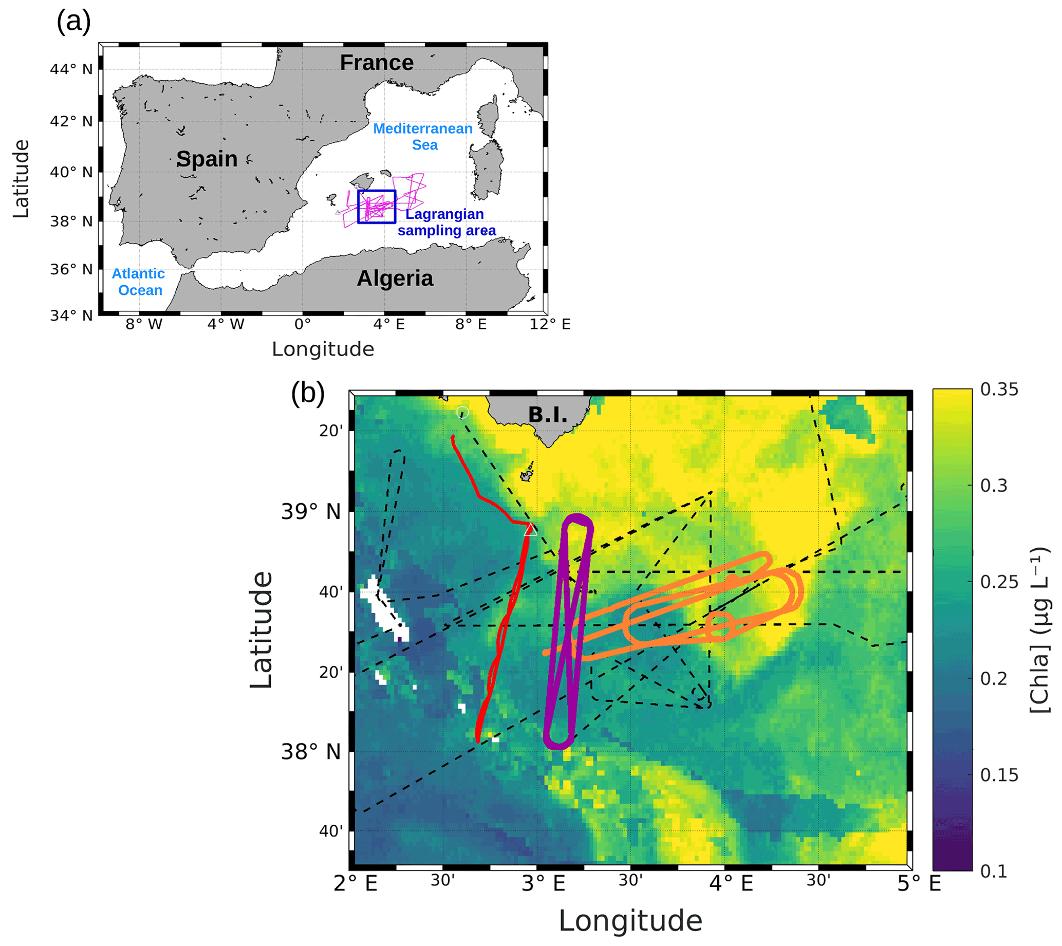
Figure 1 (a) Whole route of the RV Beautemps-Beaupré during PROTEVSMED-SWOT (pink line). The blue box corresponds to the area sampled with the Lagrangian strategy. (b) Map of satellite-derived [chl a] provided by CLS for 3 May 2018, selected in the Lagrangian sampling area and superimposed onto the route of the ship (black dotted line). The orange and purple lines delineate the two areas called “hippodromes”: west–east (orange) and north–south (purple). The red line represents the route of the SeaExplorer glider.

SPASSO was used to follow both the temporal and spatial variability of the horizontal fine-scale features of interest. SPASSO combines satellite-derived currents, SST and [chl a], to provide maps of dynamical and biogeochemical structures in both near real time (NRT) and delayed time (DT). During the cruise, the analysis of these maps suggested the presence of two different regions, characterized by their different surface [chl a] (Fig. 1). Consequently, these two regions were sampled along a designated route of the ship, represented in purple and in orange in Fig. 1. Special attention was paid to adapting the temporal sampling in these different water masses to the biological timescales, i.e., to trying to catch the diurnal cycle. The shape depicted by the ship's track led us to call these areas west–east (WE) hippodrome (in orange in Fig. 1) performed from 8 to 15 May at 15:30 to 10 May at 17:30 UTC and north–south (NS) hippodrome (in purple in Fig. 1) performed between 11 May at 02:00 and 13 May at 08:30 UTC.

2.2 In situ measurements

Physical and biological variables (horizontal velocities, temperature, salinity and abundances of the different phytoplankton functional groups) were measured at high frequency all along the route. In situ systems included a SeaSoar deployed at sea, a vessel-mounted acoustic Doppler current profiler (VMADCP), a thermosalinograph (TSG) and a flow cytometer installed on board. The SeaSoar is a towed undulating vehicle capable of achieving undulations from the surface down to 400 m. Two Sea-Bird SBE-9 (with SBE-3 temperature and SBE-4 conductivity sensors) instruments mounted on either side of the SeaSoar enabled simultaneous measurements of temperature, salinity (from conductivity) and pressure. The conductivity and temperature data were lag-corrected to reduce salinity spiking following the methodology developed by Lueck and Picklo (1990), Morison et al. (1994) and Mensah et al. (2009), before conversion to absolute salinity S_A and conservative temperature Θ, in accordance with TEOS-10 standards (McDougall et al., 2012). Herein, temperature and salinity refer to absolute salinity and conservative temperature. Horizontal velocities between 19 and 253 m were measured with a VMADCP operating at 150 kHz. VMADCP data treatment was performed with the MATLAB software Cascade V.7 (https://www.umr-lops.fr/en/Technology/Software/CASCADE-7.2, last access: 3 December 2021). The sea surface temperature and salinity were measured continuously along the ship route by the underway TSG. The TSG was equipped with two sensors: (i) a CTD Sea-Bird Electronics SBE 45 sensor, which was installed in the wet lab, was connected to the surface water and which continuously pumped seawater at 3 m depth; and (ii) an SBE 38 temperature sensor, which was installed at the entry of the water intake.

An automated CytoSense flow cytometer (CytoBuoy b.v.) was installed on board and connected to the seawater circuit of the TSG to perform scheduled automated sampling and analysis of phytoplankton (Thyssen et al., 2009, 2015). The instrument contains a sheath fluid made of 0.1 µm filtered seawater, which stretches the sample in order to separate, align and drive the individual particles (i.e., cells) through a light source. This light source is composed of a 488 nm laser beam. When the particles cross the laser beam, they interact with the photons. Several optical signals are recorded for each individual particle: the forward angle light scatter (FWS) and 90^∘ sideward angle scatter (SWS), related to the size and the structure (granularity) of the particles. Two signals of fluorescence induced by the light excitation were also recorded: a red fluorescence (FLR) induced by chlorophyll a and an orange fluorescence (FLO) induced by the phycoerythrin pigment. Two distinct protocols were run sequentially every 30 min, in order to process the 1164 samples. The first protocol (FLR6) had an FLR trigger threshold fixed at 6 mV and could analyze a volume of 1.5 cm³. It was dedicated to the analysis of the smaller phytoplankton such as Synechococcus, which were optimally resolved and counted with this protocol. The second protocol (FLR25) targeted nanophytoplankton and microphytoplankton with an FLR trigger level set at 25 mV and an analyzed volume of 4 cm³. The data were acquired using the USB software (CytoBuoy b.v.) but were analyzed with the CytoClus software (CytoBuoy b.v.). The combination of the different variables recorded by the flow cytometer exhibited various clusters of particles (cells) whose abundance (cells per cubic centimeter) and average variable intensities were provided by the CytoClus software, which generated several two-dimensional cytograms (e.g., Fig. 6; see Sect. 3.3 for explanation of the group identification) of retrieved information from the four pulse-shaped curves (FWS, SWS, FLO, FLR) obtained for each individual cell.

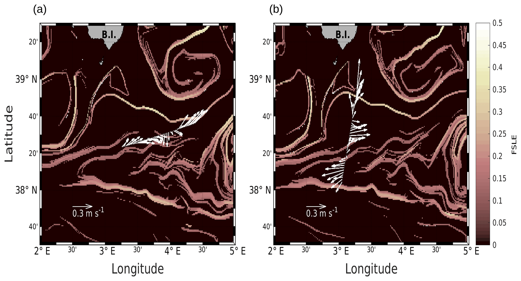
Figure 2 Horizontal velocities measured by VMADCP at 25 m, along the WE (a) and NS (b) transects, superimposed onto the FSLE field for the corresponding date (i.e., 9 and 11 May 2018, respectively). Unit for FSLE is d⁻¹.

On 5 May 2018, a SeaExplorer glider, manufactured by Alseamar (code name: SEA003), was deployed at sea. After a short transit, it performed a route approximately parallel to the NS hippodrome (red track in Fig. 1). This glider was programmed to dive to 650 m depth and was equipped with a pumped conductivity–temperature–depth sensor (Sea-Bird's GPCTD) from which the conservative temperature (Θ), the absolute salinity (S_A) and the density anomaly referenced to the surface (σ₀) were derived using the TEOS-10 toolbox (McDougall and Barker, 2011). This GPCTD was also equipped with a dissolved oxygen (O₂) sensor (Sea-Bird's SBE-43F) to measure oxygen concentrations. In addition, the glider carried a WET Labs ECO Puck FLBBCD for measurements of (i) [chl a] fluorescence (targeting excitation and emission wavelengths at λEx/λEm: 470/695 nm), converted into chl a concentrations (in micrograms per liter); (ii) backscattering at 700 nm (BB700); and (iii) a FDOM fluorophore, namely the humic-like fluorophore or peak C in the Coble (1996) classification (λEx/λEm: 370/460 nm), expressed in micrograms per liter equivalent quinine sulfate units (micrograms per liter QSU). Finally, the SeaExplorer was also equipped with two MiniFluo-UV fluorescence sensors (hereafter called MiniFluo) for the detection of various FDOM fluorophores (Cyr et al., 2017, 2019). In this study, the MiniFluo-1 was used for the detection of tryptophan-like fluorophore (λEx/λEm: 275/340 nm), while the MiniFluo-2 was used for the detection of tyrosine-like fluorophore (λEx/λEm: 260/315 nm). Tryptophan- and tyrosine-like fluorophores, referred to as peak T and peak B, respectively, in the Coble (1996) classification, are amino-acid-like components commonly found in the marine environment and generally associated with autochthonous biological processes (see review by Coble et al., 2014). Here, fluorescence intensities of tryptophan- and tyrosine-like fluorophores are provided in relative units (RU) and are not converted into mass concentration (microgram per liter) (Cyr et al., 2017, 2019). Glider observations were processed with the Socib glider toolbox (Troupin et al., 2015) for cast identification and geo-referencing.

2.3 Vertical velocity estimation

Vertical velocity was estimated using the so-called quasi-geostrophic (QG) omega Eq. (1) (Hoskins et al., 1978; Tintoré et al., 1991; Allen and Smeed, 1996):

$$\begin{array}{}\text{(1)}& {\mathrm{\nabla }}^{\mathrm{2}}\left(N^{\mathrm{2}}w\right)+f^{\mathrm{2}}{\displaystyle \frac{{\partial }^{\mathrm{2}}w}{\partial z^{\mathrm{2}}}}=\mathrm{2}\mathrm{\nabla }\cdot \mathit{Q},\end{array}$$

where w is the vertical component of the velocity field and Q is the vector determined by the horizontal derivatives of water density and horizontal velocity Eq. (2) (Hoskins et al., 1978; Giordani et al., 2006):

$$\begin{array}{}\text{(2)}& \mathit{Q}=\left({\displaystyle \frac{g}{{\mathit{\rho }}_{\mathrm{0}}}}{\displaystyle \frac{\partial {\mathit{V}}_{\text{g}}}{\partial x}}\mathrm{\nabla }\mathit{\rho },{\displaystyle \frac{g}{{\mathit{\rho }}_{\mathrm{0}}}}{\displaystyle \frac{\partial {\mathit{V}}_{\text{g}}}{\partial y}}\mathrm{\nabla }\mathit{\rho }\right),\end{array}$$

with V_g the geostrophic horizontal velocity vector, ρ the density, ρ₀ a reference density equal to 1025 kg m⁻³, g the gravitational acceleration, f the Coriolis parameter (considered constant and computed at the mean latitude of the area) and N² the Brunt–Väisälä frequency. The QG theory is valid for low Rossby numbers, a condition that is satisfied in this study.

Figure 3 Maps of vertical velocities at (a) 25 m and (b) 85 m. Black lines represent the σ contours. The data have been selected where the error on the objective mapping of σ is ≤0.0025.

High-resolution in situ data are necessary to solve Eq. (1). In this work, σ was obtained from SeaSoar CTD measurements (Fig. A1), and the geostrophic component of the horizontal velocity was estimated from the measurements performed with the VMADCP as in the work of Barceló-Llull et al. (2017). Following suggestions made by Allen et al. (2001) to preserve synopticity as much as possible, we selected four transects of the NS hippodrome (see Fig. 1) between 11 and 12 May 2018 in order to obtain a “butterfly” design as in Cotroneo et al. (2016) and Rousselet et al. (2019). The σ, u and v fields were interpolated onto a 3D grid, using objective analysis (Le Traon, 1990; Rudnick, 1996). The horizontal grid resolution is 0.9 km × 0.9 km, and the vertical resolution is 6 m (from 19 to 253 m depth). We followed the method described by Rudnick (1996), using the scripts freely downloadable from his web page at http://chowder.ucsd.edu/Rudnick/SIO_221B.html (last access: 3 December 2021). The in situ data are considered to be composed of a mean value, a fluctuation and some noise including both smaller-scale variability and instrument error. The fluctuation part of the field statistics was assumed to have a decorrelation length scale of 20 km in both the x and y directions, with a structure orientation of 18.4^∘ from north. The correlation length scale was chosen by analyzing the auto-covariance matrix of the σ field and performing several sensitivity tests. The noise-to-signal ratio was assumed to be 0.05, as in Rudnick (1996). The interpolated fields are shown superimposed onto the in situ measurements (see Fig. A1 in the Appendix). The ageostrophic component of the velocity measured by the VMADCP was then removed and Eq. (1) was solved with an iterative relaxation method and constrained by Dirichlet boundary conditions (w=0), as in the case of the front studied by Rudnick (1996). To minimize the effect of the imposed boundary conditions, only data with an error on the objective mapping of σ≤0.0025 were then considered.

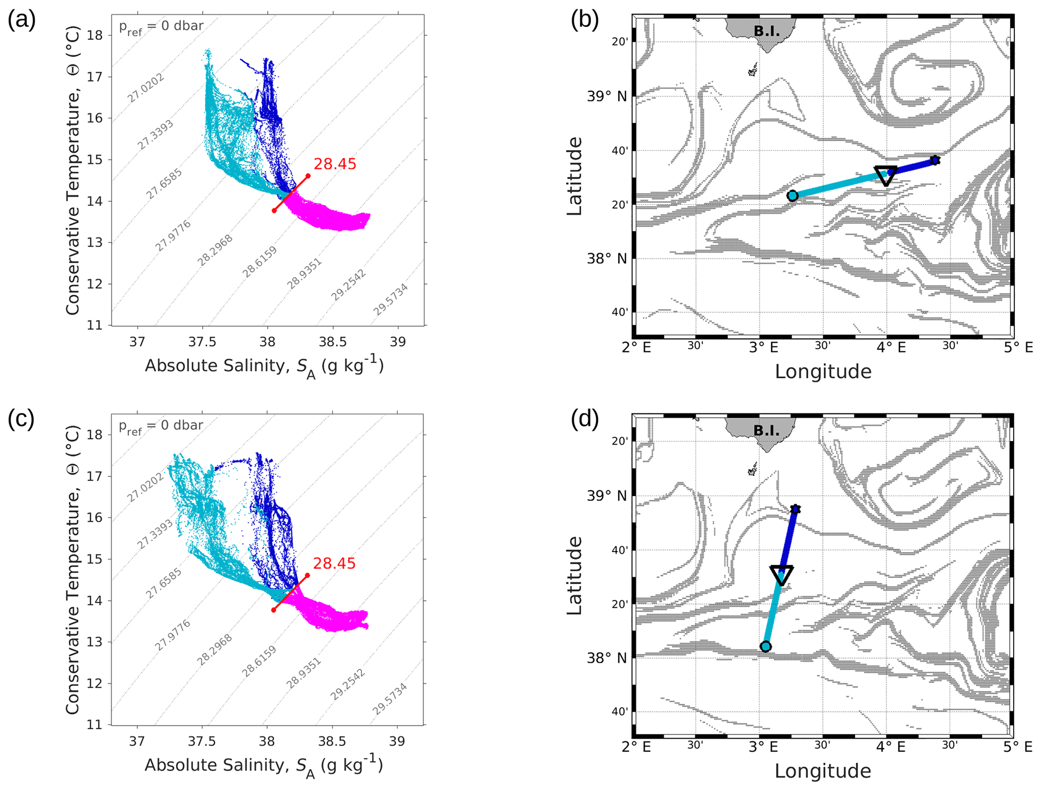
Figure 4 Θ–S_A diagrams of data collected along the WE (a) and the NS (c) transects. The younger AW is represented in light blue and the older AW in dark blue. Intermediate water is also represented in pink. The isopycnal 28.45 kg m⁻³, separating surface waters from the deeper ones, is highlighted in red. Triangles in panels (b) and (d) indicate the geographical position of the separation between the two types of AW along the corresponding transect.

3 Results

3.1 Hydrodynamics

We will first describe the hydrodynamic conditions encountered during PROTEVSMED-SWOT in order to characterize the area. For simplicity, two transects only, representative of each of the two hippodromes, are described: the first transect, on the WE hippodrome and performed from 16:50 to 23:45 UTC on 9 May, is referred to as the WE transect (Fig. 2a). The second one, performed on the NS hippodrome from 02:00 to 08:40 UTC on 11 May, is referred to as the NS transect (Fig. 2b). Note that we obtained similar results for the other transects (see Fig. A2 in the Appendix). The horizontal velocities were measured by VMADCP at 25 m along both WE and NS transects and superimposed onto the FSLE field for the corresponding date. The intensity and the direction of the current vary along the transects. A slowly evolving zonal fine-scale feature is present at around 38^∘ 20^′ N in the altimetry-derived FSLE field and is confirmed by the VMADCP data. Indeed, two FSLE features cut the transect at this latitude, exactly where the horizontal current directions change substantially. The WE transect shows a larger current variability than the NS transect, due to its alignment with the fine-scale structure. However, an FSLE feature cuts this transect just north of 38^∘ 20^′ N where the current begins to change and turns to the northeast.

Figure 3a and b show the vertical velocities estimated at 25 and 85 m depths for the NS hippodrome. The area is characterized by three main features: two upwelling cells (positive values) separated by a downwelling cell (negative values) located between 38^∘ 30^′ N and 38^∘ 36^′ N. Another smaller downwelling patch is present in the southeast of the sampling area. The intensities of these vertical motions, ranging from 2 to $\mathrm{8}\times {\mathrm{10}}^{-\mathrm{5}}$ m s⁻¹ (corresponding to 1.7 to 6.9 m d⁻¹), are stronger in the intermediate layer.

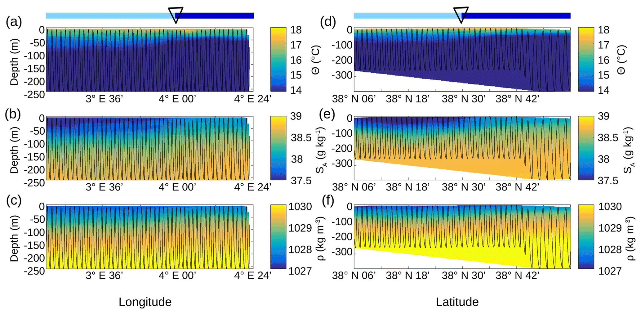
Figure 5 Vertical sections of conservative temperature Θ (a, d), absolute salinity S_A(b, e) and density ρ (c, f), sampled by the SeaSoar along the WE transect (a–c) and along the NS transect (d–f). The SeaSoar trajectory is represented by the black lines. The triangle indicates the location of the front area between the two types of AW represented in light and dark blue (see Fig. 4b and d respectively).

Table 1 Results of the iterative algorithm to determine the best separation between the two types of AW along the SeaSoar transects of the WE and NS hippodromes. The lines in bold correspond to the WE and the NS transects represented in Fig. 4. Only one transect is available for the WE hippodrome due to technical problems encountered with the towed fish.

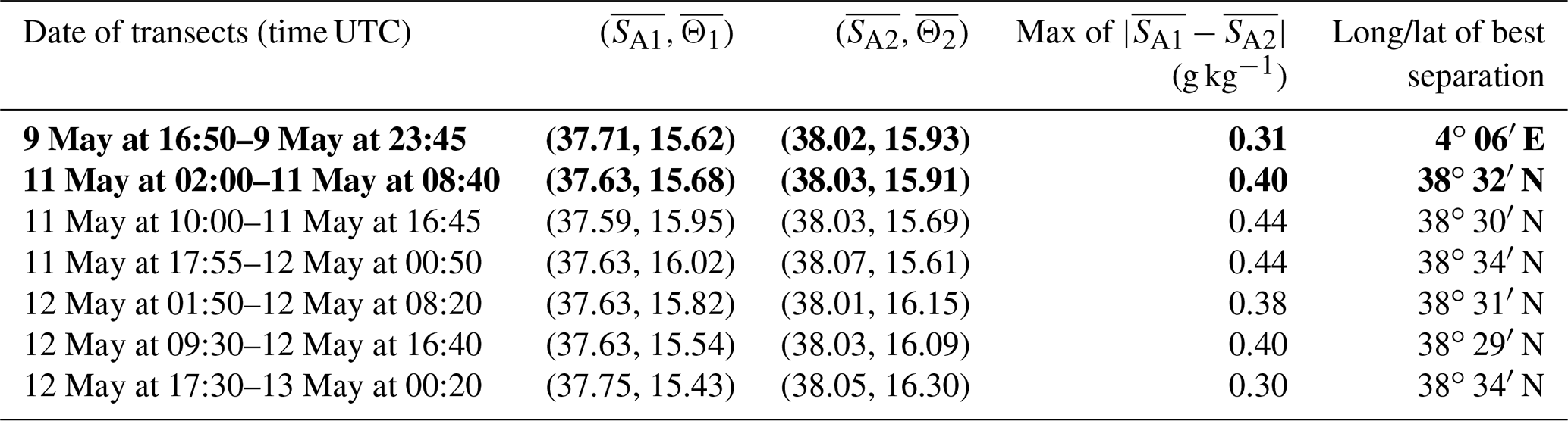
3.2 Hydrology

The typical southwestern Mediterranean water masses are shown in the Θ–S_A diagrams of the SeaSoar CTD data of the WE and NS transects (Fig. 4a and c, respectively). A clear separation into two different water masses is visible at the surface. In order to objectively identify where these two water masses separate we first distinguish surface from intermediate waters by the isopycnal at 28.45 kg m⁻³ on the Θ–S_A diagrams. Then, an iterative method with a granularity of 0.05^∘ in longitude (latitude) along the WE (NS) transect was used to calculate the means of the two surface water masses in terms of salinity and temperature, $(\stackrel{\mathrm{‾}}{S_{\text{A1}}},\stackrel{\mathrm{‾}}{{\mathrm{\Theta }}_{\mathrm{1}}})$ and $(\stackrel{\mathrm{‾}}{S_{\text{A2}}},\stackrel{\mathrm{‾}}{{\mathrm{\Theta }}_{\mathrm{2}}})$, and the difference in terms of mean salinity, $|\stackrel{\mathrm{‾}}{S_{\text{A1}}}-\stackrel{\mathrm{‾}}{S_{\text{A2}}}|$. The best separation between the two surface water masses thus corresponds to the longitude (latitude) along the WE (NS) transect where the maximal difference $|\stackrel{\mathrm{‾}}{S_{\text{A1}}}-\stackrel{\mathrm{‾}}{S_{\text{A2}}}|$ is found. Table 1 summarizes the maximal differences calculated for the transects of the WE and NS hippodromes performed with the SeaSoar and the associated localizations of the best separation. Only one transect of the WE hippodrome is shown due to a lack of data in the SeaSoar measurement during the other transects of this hippodrome. In Table 1, along the WE transect the surface water masses separate at longitude 4^∘ 06^′ E, while along the NS transect they separate at latitude 38^∘ 32^′ N, as is also indicated by the triangles on the corresponding figures (Fig. 4b, d). Note that for the other meridional transects the estimated separation varies by a few minutes only (Table 1). Θ–S_A diagrams (Fig. 4a, c), and their associated maps (Fig. 4b, d) correspond to the WE and the NS transects described previously in Sect. 3.1. The maps shown in Fig. 4b and Fig. 4d indicate the geographical positions of the two types of Atlantic Water (AW), using the same color code as in the Θ–S_A diagrams. Interpretation of these data is as follows: the surface layer is occupied by AW with different residence times in the Mediterranean Sea. We refer to these two AWs as “younger AW” (in light blue) and “older AW” (in dark blue). The younger AW corresponds to AW which has entered the Mediterranean basin more recently and which is characterized by a salinity between 37 and 38 g kg⁻¹, while the older AW is characterized by a higher salinity. Previous authors have referred to this water as “local AW” (Barceló-Llull et al., 2019) or “resident AW” (Balbín et al., 2012). The younger AW is located at the west and at the south of the WE and NS transects, respectively. Moreover, the separation between the two types of AW is in agreement with the localization of the front identified by the FSLE and the change in the current direction (Fig. 2).

This separation between the two types of AW is also visible on the SeaSoar vertical sections of conservative temperature, absolute salinity and density (Fig. 5). Examination of the gradients along the temperature (Fig. 5a, d) and salinity (Fig. 5b, e) transects enables us to clearly identify the separation between the two types of AW at longitude 4^∘ E for the WE transect and latitude 38^∘ 30^′ N for the NS transect, corresponding to the localization of the front. However, this separation is less apparent along the two density transects (Fig. 5c, f). Furthermore, the vertical extension of the surface and intermediate water masses is also visible on the vertical SeaSoar sections along the WE and NS transects (Fig. 5). The warm surface layer with temperature greater than 15 ^∘C extends to about 100 m (Fig. 5a, d). This layer is also characterized by a salinity between 37.5 and 38 g kg⁻¹ (Fig. 5b, e) and, as a consequence, by the lowest density (Fig. 5c, f). Note that this surface layer is more apparent along the WE transect (Fig. 5a, b, c) than along the NS transect. Below 100 m depth, the intermediate water is more homogeneous and is characterized by a temperature of 13–14 ^∘C and a salinity of 38–38.5 g kg⁻¹ (in pink in Fig. 4a, c).

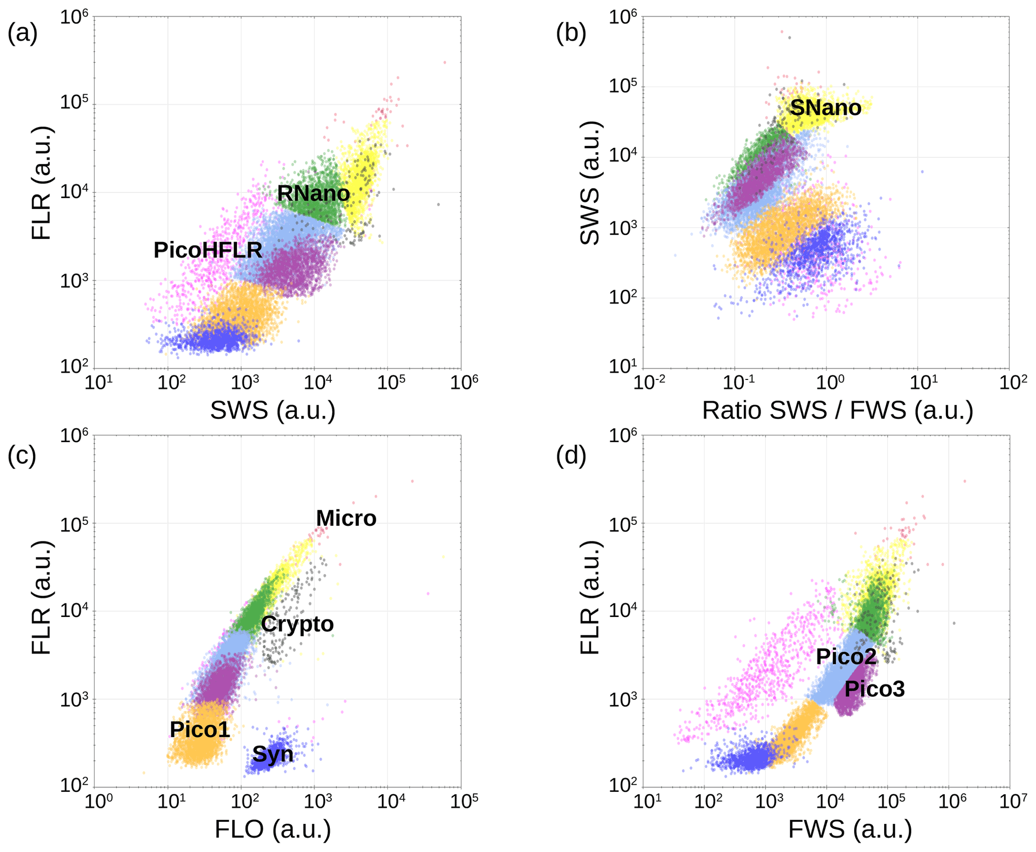
Figure 6 Cytograms obtained with the CytoSense automated flow cytometer. Synechococcus are in dark blue (Syn), the picophytoplankton with lowest FLO in orange (Pico1), the picophytoplankton with intermediate FWS in light blue (Pico2), the picophytoplankton with highest FWS in purple (Pico3), the picophytoplankton with a high red fluorescence in pink (PicoHFLR), the nanophytoplankton with high SWS $/$ FWS ratio in yellow (SNano) and higher SWS intensities than the other nanophytoplankton (RNano) in green, the cryptophytes in grey (Crypto), and the microphytoplankton in red (Micro). The flow cytometry units for both fluorescence and light scatter are arbitrary (a.u.).

The SeaExplorer glider also performed temperature and salinity measurements along a transect parallel to and slightly west of the NS hippodrome (see Fig. 1). The Θ–S_A diagrams of the glider data (Fig. A3a, b) confirm the presence of the two types of AW in surface, in particular during the outward route (Fig. A3a). During the glider's return route (Fig. A3b) the surface water masses were beginning to be more homogeneous than during the outward route and the NS SeaSoar transect (Fig. 4c). This can be explained by the fact that the SeaSoar transects were performed within a few hours, while the glider transects lasted several days. Finally, the deeper glider sampling allowed us to detect another thermohaline signature, with temperature values about 13 ^∘C and salinity about 38.5 g kg⁻¹, corresponding to Western Mediterranean Deep Water (WMDW) as found by Balbín et al. (2012).

3.3 Characterization and distribution of phytoplankton by flow cytometry

Up to nine phytoplankton groups were optically resolved by flow cytometry (Fig. 6). The light scatter (forward scatter, FWS; and sideward scatter, SWS) and fluorescence intensities (red fluorescence, FLR; and orange fluorescence, FLO) were used to identify these nine phytoplankton groups, following Thyssen et al. (2015) and Marrec et al. (2018). We called these groups by the conventional names used by flow cytometrists, i.e., some groups relate to taxonomy (Synechococcus, cryptophytes), while others relate to a range of sizes (picoeukaryotes, nanoeukaryotes) following Sieburth et al. (1978). Indeed, the first group corresponds to Synechococcus (Syn in Fig. 6c), which is a prokaryotic picophytoplankton. We distinguish Synechococcus from the other picophytoplanktonic groups, because it was evidenced by flow cytometry thanks to its higher FLO intensity compared to FLR intensity (Fig. 6c), induced by the presence of phycoerythrin pigments. A first eukaryotic picophytoplankton group (Pico1) shows lower FLR and FLO intensities than Synechococcus (Fig. 6c). Two other groups of picophytoplankton (Pico2 and Pico3) exhibit higher FWS, SWS and FLR intensities than Pico1 (Fig. 6d). The last group of picophytoplankton (PicoHFLR) is characterized by a high FLR signal induced by chl a. Two distinct nanophytoplankton groups (SNano and RNano) were defined according to their high FLR and FLO intensities (Fig. 6a, c). SNano nanophytoplankton have a high SWS $/$ FWS ratio and higher SWS intensities than RNano (Fig. 6a, b). Finally, microphytoplankton (Micro) and cryptophytes (Crypto) exhibit high FLR and FLO intensities (Fig. 6c). Cryptophytes can belong to the picoeukaryotes or nanoeukaryotes but have also been discriminated from the red-only fluorescing picoeukaryotes or nanoeukaryotes based on their orange fluorescence induced by phycoerythrin, like Synechococcus. The size and the abundances of these nine groups are summarized in Table 2.

Table 2 Size and abundances of the nine phytoplankton groups, identified by flow cytometry analysis in Fig. 6.

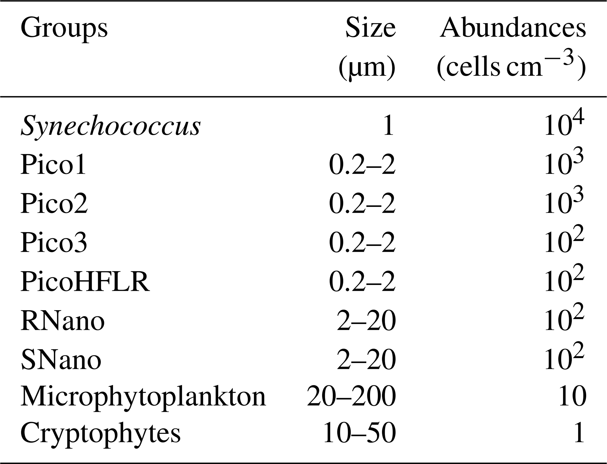
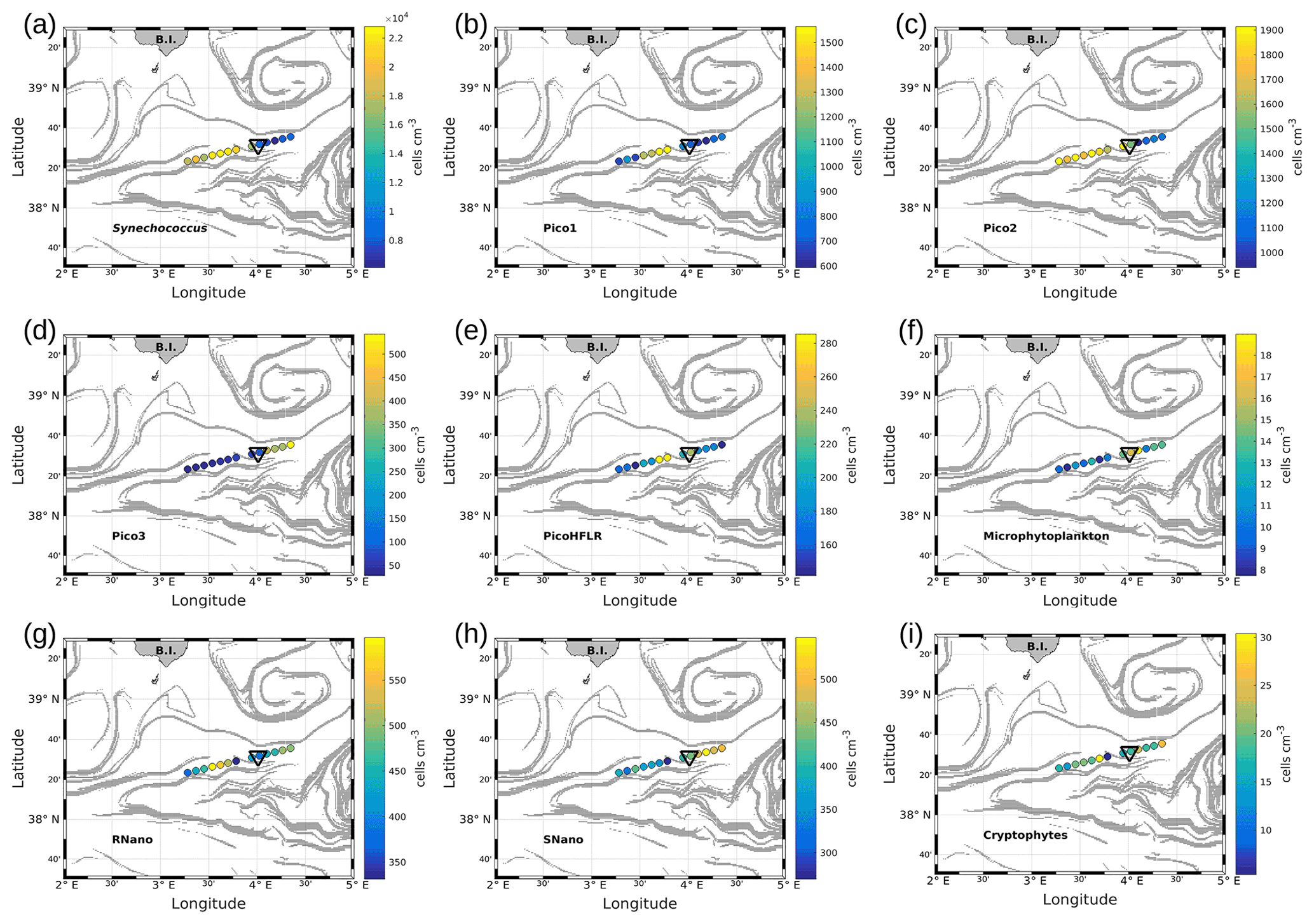
Figure 7 Abundances (in cells per cubic centimeter) of the phytoplankton groups along the WE transect, superimposed upon the FSLE field. Triangles indicate the front area. (a) Synechococcus, (b) Pico1, (c) Pico2, (d) Pico3, (e) PicoHFLR, (f) microphytoplankton, (g) RNano, (h) SNano and (i) cryptophytes.

Figures 7 and 8 show the surface abundances of the various phytoplankton groups, along the WE and the NS transects. Synechococcus (Figs. 7a and 8a), Pico1 (Figs. 7b and 8b) and Pico2 (Figs. 7c and 8c) present a similar distribution pattern. High abundances around 2.2–3.0×10⁴, $\ge \mathrm{1.1}\times {\mathrm{10}}^{\mathrm{3}}$ and $\ge \mathrm{1.7}\times {\mathrm{10}}^{\mathrm{3}}$ cells cm⁻³, recorded respectively for Synechococcus, Pico1 and Pico2, are located at the western and southern parts of the front, along with the WE and the NS transects. On the other side of the front, their abundances are lower ($\le \mathrm{1}\times {\mathrm{10}}^{\mathrm{4}}$ cells cm⁻³ for Synechococcus and ∼ 500 and ∼ 900 cells cm⁻³ for Pico1 and Pico2, respectively). RNano abundances (Figs. 7g and 8g) present a similar distribution with these groups along the NS transect, with high abundances (450–500 cells cm⁻³) located at the southern part of the front. However, the distribution of RNano abundances is less clear along the WE transect. Pico3 (Figs. 7d and 8d), microphytoplankton (Figs. 7f and 8f) and SNano (Figs. 7h and 8h) abundances vary between 100–500, 8–18 and 300–500 cells cm⁻³, respectively, and present an opposite distribution compared to the other groups. Indeed, higher abundances are found in the eastern and northern parts of the front. PicoHFLR (Figs. 7e and 8e) and cryptophyte abundances (Figs. 7i and 8i) ranged from 160–280 and 10–30 cells cm⁻³ respectively. However, the latter exhibited a less obvious pattern between the two sides of the front. Overall, the distribution of the abundances of the various phytoplankton groups evidenced by flow cytometry on either side of the front (except for these two last groups) fits well with the hydrodynamic and hydrological observations.

3.4 Statistical analysis

Surface temperature and salinity data measured with the TSG were merged with abundance data of the nine phytoplankton groups at each cytometry sampling point along the WE and NS hippodromes. Thus, the final data set consists of 11 variables, each of which contains 215 observations. To deal with this large multivariate data set a principal component analysis (PCA) was applied.

PCA consists of summarizing the information contained in the data set by replacing the initial variables with new synthetic variables (called principal components), which are linear combinations of the initial variables and uncorrelated two by two. When applied to our data set, a PCA reveals that the first three components account for 36.7 %, 18.1 % and 13 % of the total variance of the data, respectively. The following statistical analysis focuses on these three components, representing 67.8 % of the total variance of the data. Figure 9a shows positively correlated variables grouped together in the first factorial plane: salinity (S_A) with microphytoplankton (Micro); Synechococcus (Syn) with picophytoplankton Pico1 group, picophytoplankton Pico2 group and nanophytoplankton RNano group; and temperature (Θ) with picophytoplankton Pico3 group and nanophytoplankton SNano group. However, the cryptophytes (Crypto) group and the picophytoplankton PicoHFLR group are less well correlated with the other variables compared to the other groups of phytoplankton.

The K-medoid algorithm, described by Hartigan and Wong (1979) and Kaufman and Rousseeuw (1987), is another method used to represent the various aspects of the data structure. This algorithm divides M points in N dimensions into K groups (or clusters). A cluster is an object for which the average dissimilarity to all the data is minimal. In our case study, the K-medoid algorithm splits the 215 points (i.e., observations) into three clusters (Fig. 9b). Each point of a given cluster shows a high degree of similarity with the others points of the same cluster. The three clusters are well separated from each other. Only a few points of the black and red clusters are difficult to unravel. Finally, the average of each variable called local average and the global average can be calculated for each cluster to show the contribution of each variable to a cluster. The most discriminating variables for each cluster (Table 3) were also determined with the standard deviation.

Figure 8 As in Fig. 7 but for the NS transect.

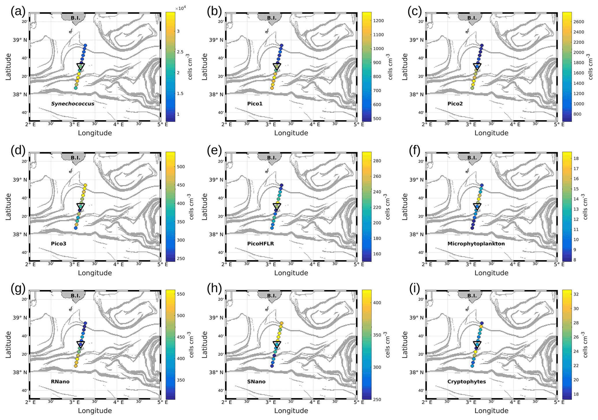
Figure 9c is a spatiotemporal representation of the three main clusters obtained by the K-medoid algorithm. The WE hippodrome from 8 to 10 May is characterized by the presence of the black cluster in the east and the red cluster in the west. The NS hippodrome starts on 11 May, with the red cluster present in the south and the black cluster in the north. The latter remains dominant in the north for the remainder of the sampling period. In the south, the red cluster is gradually replaced by the blue cluster, except for a few points on 13 May.

Table 3 Description of the three clusters obtained with the K-medoid algorithm and represented in Fig. 9b, c and d. The local averages (i.e., the average of each variable in a cluster) are compared with the global average (i.e., the average of each variable for the complete data set) to highlight the contribution of each variable to a cluster. Note that only the five most discriminating variables, determined with the standard deviation, are shown for each cluster. Absolute salinity is measured in grams per kilogram, conservative temperature in degrees Celsius and phytoplankton abundances in cells per cubic centimeter. The bold lines represent the variables with the greatest contribution to each cluster (i.e., with local average > global average).

Figure 9d displays the geographical distribution of the three clusters superimposed upon the FSLE field. It evidences a general good agreement between the shifts of the clusters and the FSLE maxima. In particular, the separation between the black and red clusters at around 4^∘ E on the WE hippodrome corresponds to the two FSLE maxima crossing this longitude at 38^∘ 40^′ N and 38^∘ 20^′ N. On the NS hippodrome, the black cluster is separated from the two others at about 38^∘ 20^′ N where zonally disposed FSLE maxima cross the vessel route. To summarize, the black cluster dominates in the north of the sampled area, while in the south the red cluster is dominant at the beginning before being replaced by the blue cluster. The separation between the clusters matches the distribution of the FSLE field maxima and can be explained by the fine-scale dynamics. Given their ephemeral nature the fine-scale structures, the temporal evolution of the distribution of the red and blue cluster is probably due to the displacement over time of the frontal structure during the cruise.

4 Discussion

4.1 Physical properties of the front

During the PROTEVSMED-SWOT cruise, the satellite-derived surface [chl a] showed contrasted values between the southwest and the northeast of the studied area (Fig. 1). The analysis of ocean color images combined with the altimetry-derived FSLE field has been associated with the strong variation of current direction observed in the horizontal velocities measured by VMADCP data, allowing the identification of a frontal area located at about 38^∘ 30^′ N latitude and between 3 and 4^∘ E longitude (Fig. 2).

Our estimation of vertical velocities using the omega equation method has allowed us to investigate the vertical dynamics in the frontal area (Fig. 3). Several previous studies have shown the importance of fine-scale dynamics in generating vertical velocities (e.g., Rudnick, 1996; Lapeyre and Klein, 2006; Mahadevan and Tandon, 2006; Balbín et al., 2012). Although the ship route was designed mainly with an eye to cytometry sampling across the front, we obtained a sufficiently regular spatial grid to allow us to apply the omega equation method, as Allen et al. (2001). In the area where our SeaSoar sampling overlapped with CTD casts performed on a 10 km regularly space grid by Barceló-Llull et al. (2018), the respective estimations of the vertical velocity field are in good agreement (Barceló-Llull et al., 2021). As our sampling area extends further south with respect to that of Barceló-Llull et al. (2018), we were also able to observe the shift in current direction, from eastward to westward, and the associated vertical recirculation pattern. Vertical velocities associated with the front are in the order of a few meters per day. These values are of the same order of magnitude as the velocities associated with a frontal structure reported by Balbín et al. (2012) in the northwest of the Balearic Islands and by Ruiz et al. (2019) in the Alboran Sea.

The data from the CTD sensors mounted on the SeaSoar towed fish and on the SeaExplorer ocean glider reveal a rapid shift between two different types of surface water masses on the Θ–S_A diagrams (Figs. 4 and A3). These water masses are AW at different stages of modification. Indeed, AW enters the Mediterranean Sea through the Strait of Gibraltar and then forms a counterclockwise circulation along the continental slope of the western Mediterranean basin, caused by the combination of the Coriolis effect and the topographical forcing (Millot, 1999; Millot and Taupier-Letage, 2005; Millot et al., 2006). In the southwest part of the basin, this circulation is dominated by the Algerian Current (AC), which can form meanders and mesoscale eddies due to baroclinic and barotropic instabilities (e.g., Millot, 1999). These eddies spread over the basin and join the study area south of the Balearic Islands, carrying with them the newly arrived AW, known as younger AW. In this region, the younger AW encounters the older AW, i.e., the AW modified by cooling and evaporation during its progression along the northern part of the western Mediterranean basin (Millot, 1999; Millot and Taupier-Letage, 2005). The presence of this water has already been observed by Balbín et al. (2012) and Barceló-Llull et al. (2019), who use the terms resident AW or local AW, respectively, to indicate the colder and saltier AW of the Balearic Sea.

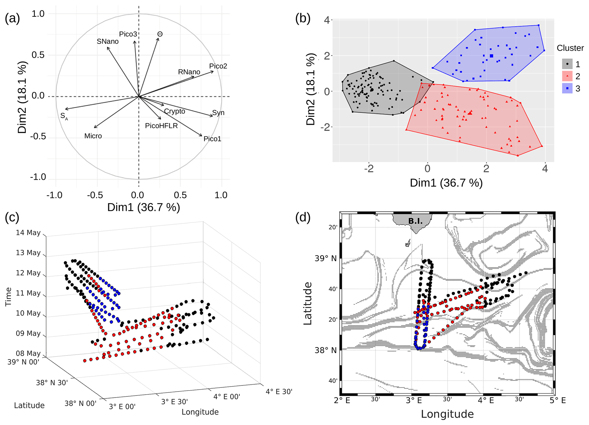
Figure 9 (a) Principal component analysis in the first factorial plane. (b) Representation in two dimensions of the three clusters obtained with the K-medoid algorithm. (c) Spatiotemporal representation of the three clusters obtained with the K-medoid algorithm. (d) Geographical representation of these clusters, superimposed upon the FSLE field, 11 May 2018.

During our cruise, the older AW and younger AW are separated by a frontal area (Fig. 4). This separation between these two AWs is also clearly visible in the first 100 m of the water column, on the depth sections of temperature and salinity (Fig. 5). López-Jurado et al. (2008) and Balbín et al. (2012, 2014) made similar observations and developed hypotheses to explain the seasonal and inter-annual variability of the location and intensity of the front between these two AWs. According to Balbín et al. (2014), the presence or absence in early summer of intermediate water in the Mallorca and Ibiza channels determines the meridional position of the front.

4.2 Biogeochemistry

Vertical sections of [chl a] and oxygen [O₂], provided by the SeaExplorer glider, were measured along the outward route (Fig. A4a, b) and the return route (Fig. A4c, d) parallel to the NS hippodrome, in the first 250 m of the water column. These glider vertical sections show patterns that can be explained by the vertical movement of the water masses. The deep chlorophyll maximum (DCM) appears to remain at a fairly constant depth along the transects. However, a deepening of the lower boundary of the layer containing the DCM is noticeable north of 38^∘ 30^′ N along the outward route (Fig. A4a) and the return route (Fig. A4c) of the SeaExplorer glider, corresponding to the older AW identified in Fig. 4d. Similar patterns also observed in the [O₂] data confirm a possible downwelling of the surface waters at the front location (see Fig. 3) but also indicate a deeper oxygenation of the older AW.

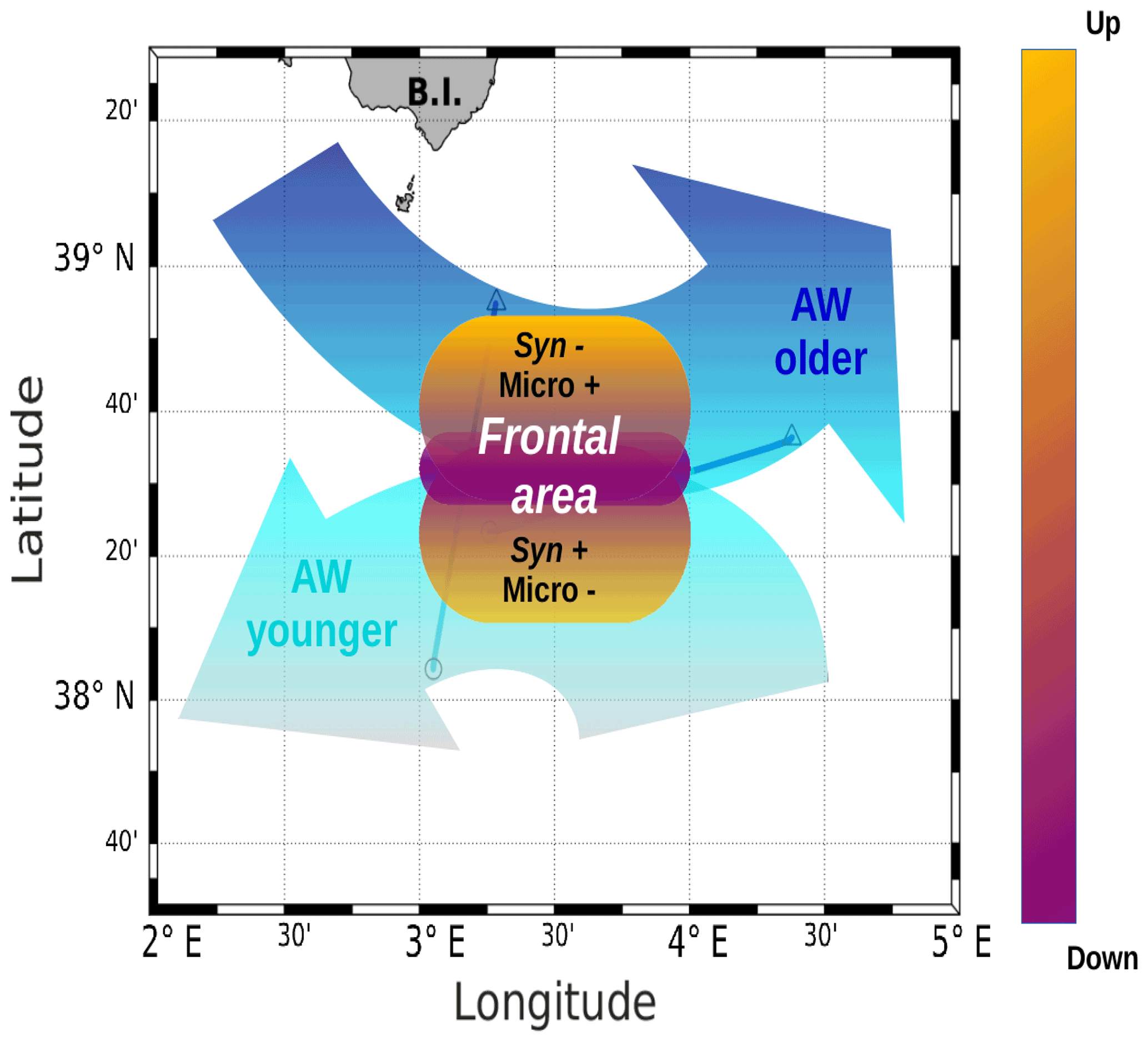
Figure 10 A schematic view of the of PROTEVSMED-SWOT results in the surface layer. A narrow frontal area, characterized by the change in direction of the horizontal current and by opposite vertical movements, corresponds to a rapid shift in hydrological properties and biological content of the two water masses separated by the front. For simplicity's sake, only two groups of phytoplankton, Synechococcus (Syn) and microphytoplankton (Micro), are indicated, but their contrasted abundances are also representative of those of other phytoplankton groups.

The vertical sections of tyrosine- and tryptophan-like fluorophores (peak B and peak T respectively) from the glider (not shown) reveal distribution patterns very close to that of [chl a] for tyrosine-like fluorophore and very close to that of [O₂] for tryptophan-like fluorophore. These similarities in the profiles of [chl a] and [O₂] were confirmed by correlation analyses (not shown), which indicate a very highly significant linear positive correlation between [chl a] and tyrosine-like fluorophores and between [O₂] and tryptophan-like fluorophores when considering all glider data for the two transects from 5 to 200 m depth (r=0.88 and 0.84, n∼32 595, p<0.0001). Tryptophan- and tyrosine-like fluorophores are recognized as having an autochthonous origin (Coble et al., 2014); as being produced through the activity of autotrophic and heterotrophic plankton organisms, in particular phytoplankton and heterotrophic bacteria (Stedmon and Cory, 2014); and as being indicators of bioavailable/labile DOM (C and N) (Hudson et al., 2008; Fellman et al., 2009). Even though phytoplankton activity is considered a source of tryptophan- and tyrosine-like fluorophores (Determann et al., 1998; Stedmon and Markager, 2005; Romera-Castillo et al., 2010), bacterial degradation appears to be not only a source, but also a sink for these fluorophores, depending on nutrient availability (Cammack et al., 2004; Nieto-Cid et al., 2006; Biers et al., 2007). The fact that tyrosine-like fluorophore was fairly associated with [chl a] and tryptophan-like with [O₂] reveals that these two fluorophores were probably not produced by the same phytoplankton groups. Moreover, it seems that tryptophan is more susceptible to release by heterotrophic bacteria (in addition to being released by phytoplankton) than is tyrosine-like material (Hudson et al., 2008; Tedetti et al., 2012; Stedmon and Cory, 2014). Figure A5 shows the comparison of distribution of [chl a] and fluorescence intensities of tyrosine- and tryptophan-like fluorophores between the younger and older AW. It appears that the content of chl a, tyrosine-like fluorophores and tryptophan-like fluorophores was higher in older AW than in younger AW (the mean values of chl a, peak B and peak T in older AW being significantly higher than those in younger AW; t test, p<0.0001). These results are in line with the distribution of microphytoplankton, which exhibited higher abundances in the northern part of the transect (older AW), thus highlighting the strong coupling between hydrology, phytoplankton activity and DOM concentration in this area.

4.3 Physical–biological coupling in the frontal area

The distribution of phytoplankton groups showed contrasted abundances across the front. Figure 10 summarizes our results, providing a view of the physical forcing occurring in the frontal area and its effect on the distribution of phytoplankton groups. The southwest of the front corresponding to the localization of the younger AW is characterized by high abundances of Synechococcus, Pico1, Pico2 and RNano groups, whereas the northeast of the front associated with the older AW is dominated by the other phytoplankton groups, i.e., Pico3, microphytoplankton and SNano (Figs. 7 and 8).

Although some studies conducted in western boundary currents have shown that fronts are sites of elevated phytoplankton diversity (Barton et al., 2010; Clayton et al., 2014), it remains unclear how physical processes impact phytoplankton distribution. In order to explain the distribution of phytoplankton abundances observed during our cruise, we can schematically separate the horizontal from the vertical processes as follows.

In terms of horizontal processes, the dominance of certain groups of phytoplankton appears well related with the type of AW. Statistical analysis proved very useful in synthesizing the physical and biological information and in identifying the relationship between some groups of phytoplankton and the hydrological water conditions. For instance, the principal component analysis (PCA) shows that Synechococcus abundance, salinity and temperature are well correlated (Fig. 9). This correlation is in accordance with the study by Mena et al. (2016), who found higher abundances of Synechococcus in the younger AW than in the older AW. Marrec et al. (2018) also revealed a dominance of Synechococcus in the warmer waters surrounding a colder cyclonic recirculation. Previous studies have shown that fine-scale ocean dynamics can drive the formation of ecological niches, by segregating water masses for long enough to create favorable conditions that permit some locally well adapted phytoplankton groups to become dominant (d'Ovidio et al., 2010; Perruche et al., 2011). d'Ovidio et al. (2010) also highlighted that these fluid ecological niches can be advected and can transport phytoplankton cells over distances far from their origin. This transport favors the creation of complex community distributions by enhancing the mingling of populations of phytoplankton. Clayton et al. (2013) reinforced this theory using global numerical simulations. According to them, dominant phytoplankton that are very well adapted locally can emerge in hotspot regions, whereas the presence of other phytoplankton called “immigrants” is sustained by physical transport. The Mediterranean spans a much reduced latitudinal gradient, and the intensity of its stronger currents allows a slower advection than that of western boundary currents. As a consequence, it is not surprising that our cytometry measurements fail to show the presence or absence of specific groups. Nevertheless, our results highlight that fine-scale dynamics modulate the relative abundance of phytoplankton groups. We can assume, for instance, that the younger AW may transport some phytoplankton cells from the Algerian Basin to the Balearic Islands. However, the front observed during our cruise cannot be defined as a hotspot of diversity as is seen in Clayton et al. (2014, 2017), where fine-scale features advect phytoplankton ecotypes that are absent in one oceanic region towards another. Our future cruises will include taxonomic analyses such as metagenomics, which will allow us to detail the structure of the communities further and better understand competition and immigration processes.

In terms of vertical processes, we can underline the role of vertical velocity (see Fig. 3). Clayton et al. (2014, 2017) highlighted the role of fine-scale circulation in regulating phytoplankton diversity. Nevertheless, they showed this in boundary currents and coastal upwelling regions and regarding opportunistic species (such as diatoms), which were fertilized by the strong nutrient enrichment induced by a very intense vertical transport. In our case, we found vertical velocities associated with the front that were less intense than those revealed by Clayton et al. (2014, 2017). This vertical transport can convey phytoplankton cells from the euphotic layer into the depths and in so doing play a key role in their distribution and their metabolism (Marrec et al., 2018). In addition to playing a role in phytoplankton distribution, vertical velocity can also advect a sufficient quantity of nutrients into the euphotic layer, creating favorable conditions for phytoplankton groups that are well adapted to the oligotrophic conditions of the Mediterranean Sea. Indeed, a previous modeling study by Lévy et al. (2001) showed the significant impact of nutrient enhancement on the phytoplankton production in an oligotrophic regime. In order to better understand these two mechanisms, additional high-resolution and high-precision nutrient measurements are needed.

5 Conclusion and perspectives

In conclusion, our adaptive Lagrangian strategy and high-resolution coupled physical–biological sampling have allowed us to detect a fine-scale frontal structure and have highlighted its structuring effect on the surface phytoplankton community, in accordance with previous modeling studies. The originality of our work resides in the fact that we have been able to demonstrate that less energetic fronts than those found in western boundary currents also have an impact on phytoplankton distribution. This suggests that the physicochemical contrasts induced by the horizontal stirring processes in moderately energetic fronts are sufficiently strong to spatially reflect into phytoplanktonic communities with different structures. Furthermore, our work offers an interesting explanation concerning the fact that despite the Mediterranean Sea being an oligotrophic regime, this region is also characterized by a high diversity of phytoplankton. Because fine-scale processes and oligotrophic regions are predominant in ocean, our results shed a new light on the functioning of the global ocean.

There remains a need for improved understanding of the biogeochemical processes generating this observed fine-scale physical–biological coupling. In particular, we plan to estimate and compare the growth rates of the various phytoplankton groups in the different water masses in future studies, using the data collected in a Lagrangian manner and applying a method similar to the one recommended by Marrec et al. (2018). Moreover, the role of nutrient supply (bottom-up) and the role of zooplankton grazing (top-down) are also key factors to be considered in explaining the variation in abundances of the diverse phytoplankton groups in the different areas visited during the cruise. To address these latter points, future experiments will involve high-resolution nutrient measurements (and also high-precision ones, considering the oligotrophy of the Mediterranean Sea), coupled with zooplankton sampling and experiments designed to improve understanding of zooplankton grazing on the different phytoplankton groups. Finally, this study highlights the value of satellite information, both in the design of the cruise sampling strategy and in the on-shore post-cruise interpretation of the data.

The new satellite SWOT (https://swot.jpl.nasa.gov/, last access: 3 December 2021; https://swot.cnes.fr, last access: 3 December 2021) will provide ocean topography and surface current data with a resolution 1 order of magnitude higher than present altimeters (Morrow et al., 2019). During the few months after its launch, throughout the so-called “fast sampling phase”, the satellite will be on a specific orbit that will overfly a portion of the global ocean and measure crossover zones, where high spatial resolution will be associated with high temporal resolution (d'Ovidio et al., 2019). The large data set collected during PROTEVSMED-SWOT represents precious new information on the SWOT crossover area located to the south of the Balearic Islands. The work presented here thus paves the way for future cruises to be planned in this area during the SWOT period, which will provide a unique opportunity for a more detailed study of physical–biological fine-scale coupling.

Appendix A

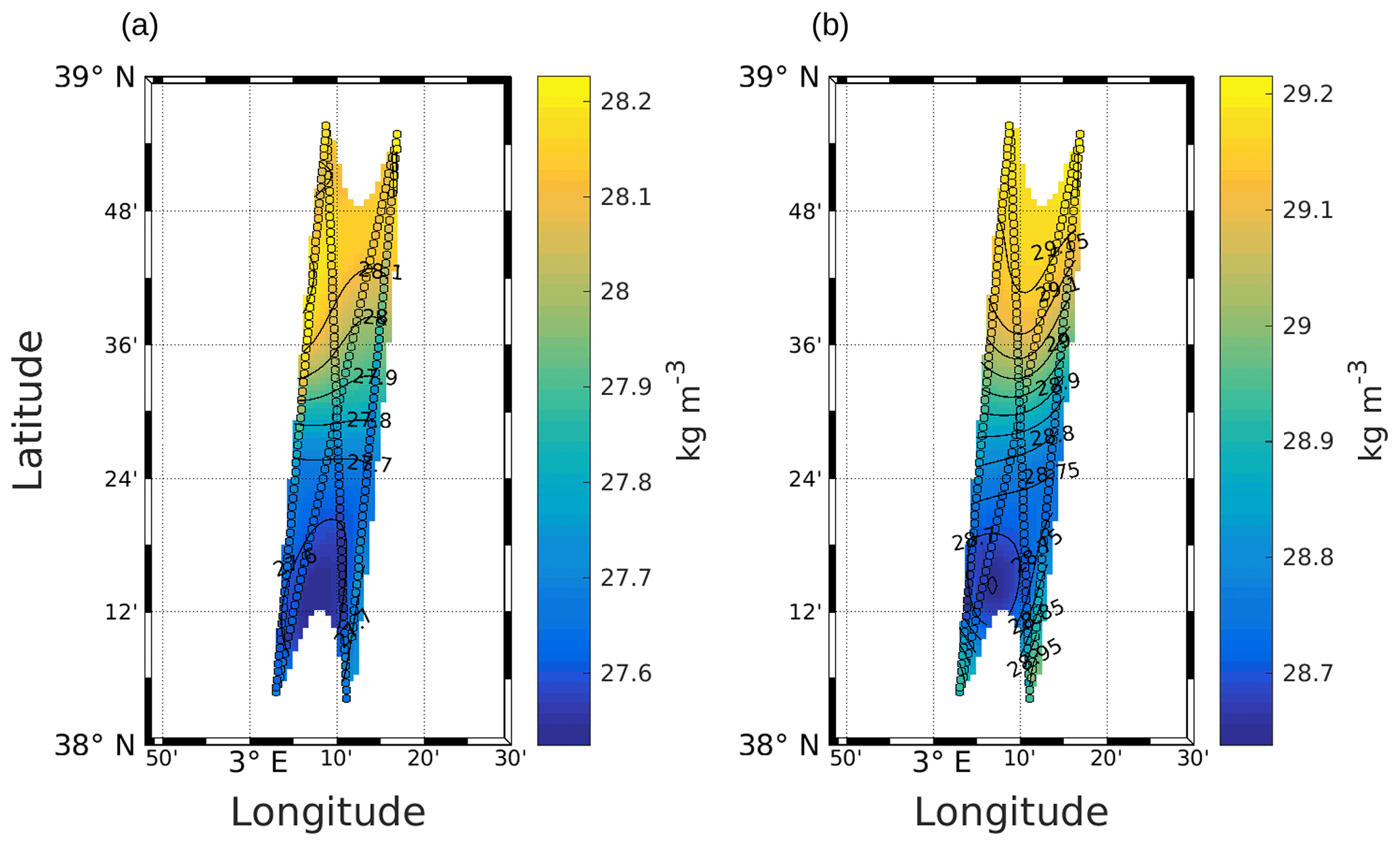
Figure A1 Objective mapping of potential density anomaly σ at 25 m (a) and 85 m (b). The circles represent σ as measured by the SeaSoar, along the transects used for the interpolation. Black lines represent σ contours. The data were selected where the error on the objective mapping of σ is ≤0.0025.

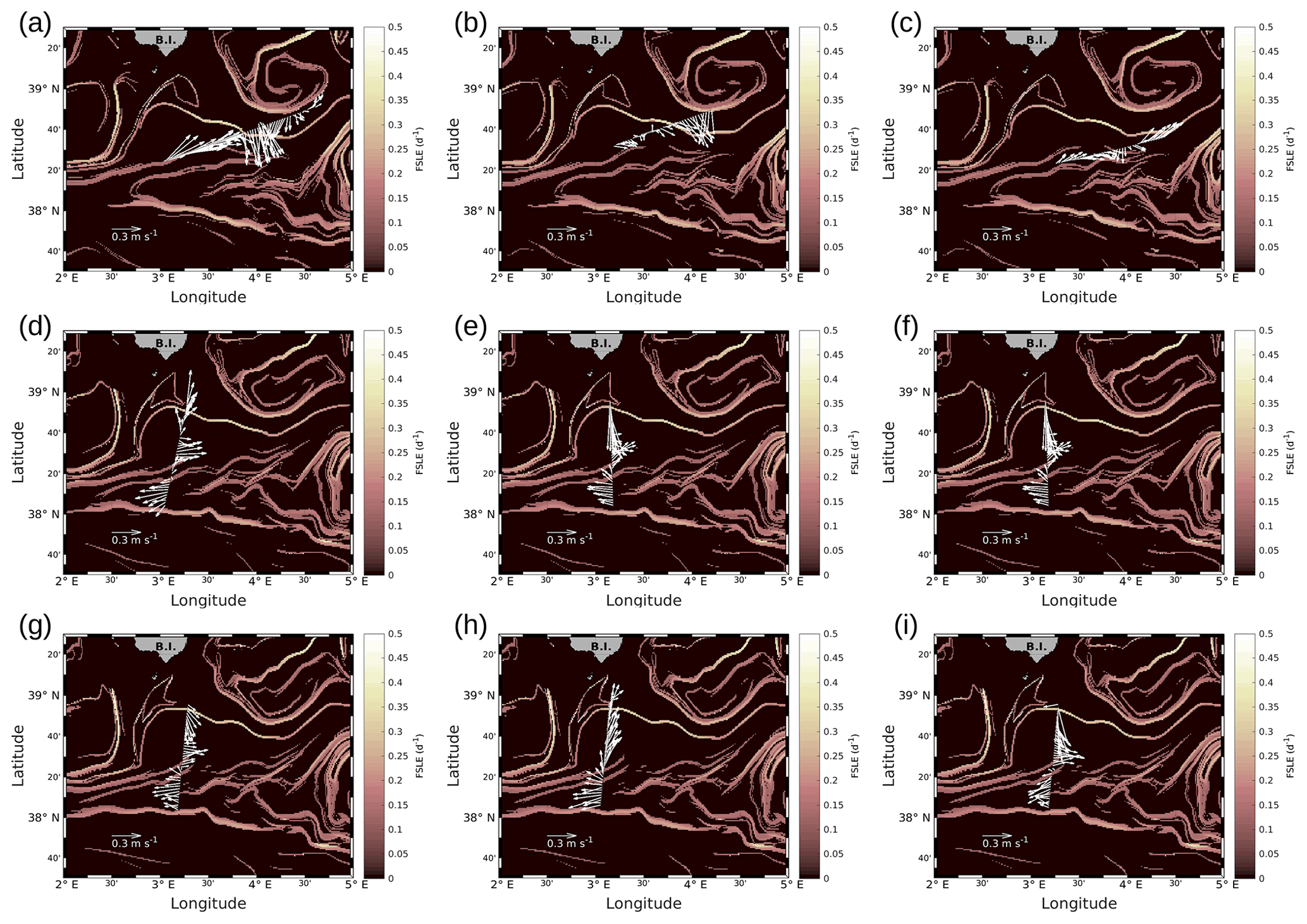
Figure A2 Horizontal velocities measured by VMADCP, along transects of the WE hippodrome (a–c) and the NS hippodrome (d–i): (a) 8 May at 12:50–9 May at 00:30; (b) 9 May at 09:00–9 May at 15:30; (c) 9 May at 16:50–9 May at 23:45; (d) 11 May at 02:00–11 May at 08:40; (e) 11 May at 10:00–11 May at 16:45; (f) 11 May at 17:55–12 May at 00:50; (g) 12 May at 01:50–12 May at 08:20; (h) 12 May at 09:30–12 May at 16:40; (i) 12 May at 17:30–13 May at 00:20. The lines in bold correspond to the WE and the NS transects described in the manuscript and also represented in Fig. 4. In our study, we have chosen to select transect (c) for the WE hippodrome, due to a lack of temperature and salinity data for the other transects of the WE hippodrome, resulting from technical problems with the SeaSoar.

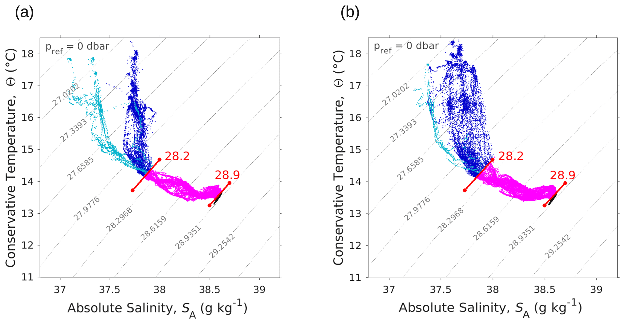
Figure A3 Θ–S_A diagrams measured by the SeaExplorer glider along the outward route (a) 6 May 2018 at 00:00–9 May 2018 at 21:00 UTC and the return route (b) 10 May 2018 at 00:00–13 May 2018 at 21:00 UTC. As in Fig. 4, the younger AW is represented in light blue, whereas the older AW is represented in dark blue. Intermediate water and deeper water are represented in pink and black, respectively. The isopycnals 28.2 and 28.9 kg m⁻³, separating surface waters from deeper water, are also shown.

Figure A4 Vertical profiles of [chl a] (a, c) and dissolved oxygen concentration (b, d), measured by the SeaExplorer glider, along the outward route (a, b) from 6 May 2018 at 00:00 to 9 May 2018 at 21:00 UTC and along the return route (c, d) from 10 May 2018 at 00:00 to 13 May 2018 at 21:00 UTC. The SeaExplorer glider trajectory is depicted by the black lines. The data were selected between the surface and 250 m for a better visualization of the surface layer.

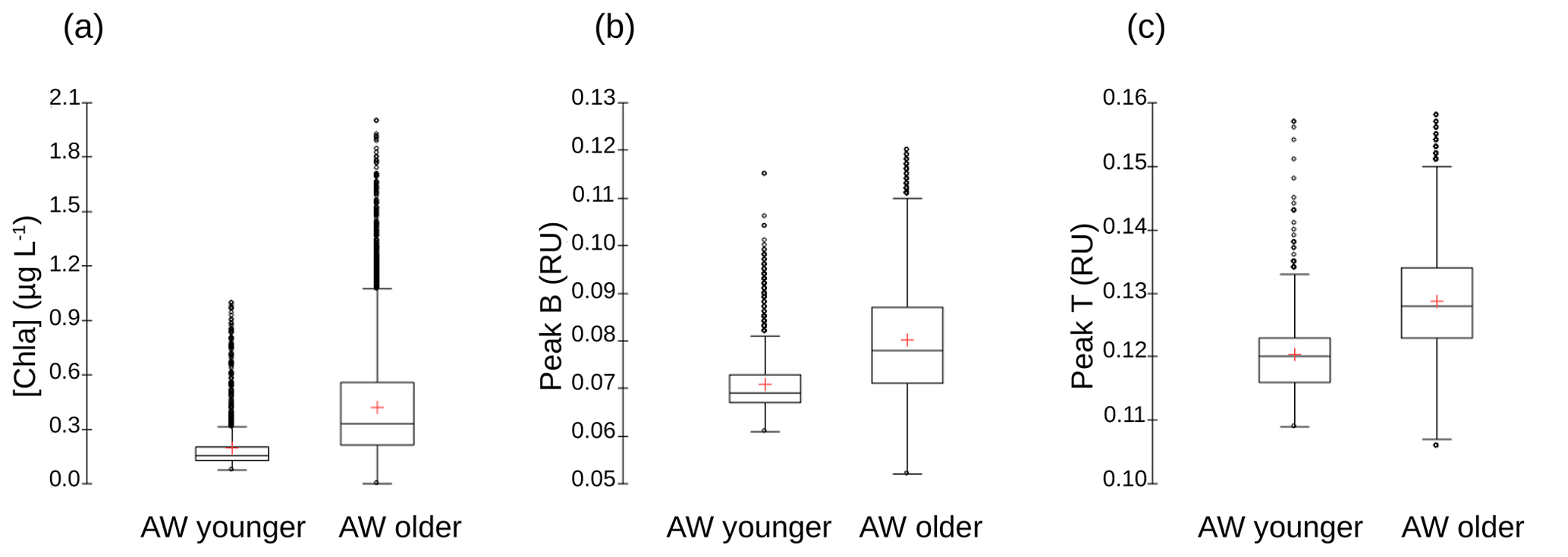
Figure A5 Box-and-whisker plots for the comparison of (a) [chl a] (in micrograms per liter), (b) fluorescence intensities of tyrosine-like fluorophore (peak B in RU) and (c) fluorescence intensities of tryptophan-like fluorophore (peak T in RU) between younger and older AW. The bottom and top of the box are the 25th and 75th percentiles, respectively, whereas the central line is the 50th percentile (the median), and the cross is the mean. The ends of the error bars correspond to the 10th percentile (bottom) and to 90th percentile (top). All the SeaExplorer glider transects are considered here (all data acquired from 6 to 15 May 2018). Younger AW corresponds to samples showing salinity between 37.20 and 37.84 and temperature between 14.5 and 17.4 ^∘C (n=1657). Older AW corresponds to samples with salinity between 37.82 and 38.14 and temperature between 14.0 and 18.3 ^∘C (n=11 760). Mean values of chl a, peak B and peak T of older AW are significantly higher than those of younger AW (t test, p<0.0001).