Resistance and resilience of stream metabolism to high flow disturbances

Streams are ecosystems organized by disturbance. One of the most frequent and variable disturbances in running waters is elevated flow. Yet, we still have few estimates of how ecosystem processes, such as stream metabolism (gross primary production and ecosystem respiration; GPP and ER), respond to high flow events. Furthermore, we lack a predictive framework for understanding controls on within-site metabolic responses to flow disturbances. Using 5 years of high-frequency dissolved oxygen data from an urban- and agricultural-influenced stream, we estimated daily GPP and ER and analyzed metabolic changes across 15 isolated high flow events. Metabolism was variable from day to day, even during lower flows; median and ranges for GPP and ER over the full measurement period were 3.7 (minimum, maximum = 0.0, 17.3) and −9.6 (−2.2, −20.5) g O₂ m⁻² d⁻¹. We calculated metabolic resistance as the magnitude of departure (M_GPP, M_ER) from the mean daily metabolism during antecedent lower flows (lower values of M represent higher resistance) and estimated resilience as the time until GPP and ER returned to the prior range of ambient equilibrium. We evaluated correlations between metabolic resistance and resilience with characteristics of each high flow event, antecedent conditions, and time since last flow disturbance. ER was more resistant and resilient than GPP. Median M_GPP and M_ER were 0.38 and −0.09, respectively. GPP was typically suppressed following flow disturbances, regardless of disturbance intensity. The magnitude of departure from baseflow ER during isolated storms increased with disturbance intensity. Additionally, GPP was less resilient and took longer to recover (0 to >9 d, mean = 2.5) than ER (0 to 6 d, mean = 1.1). Prior flow disturbances set the stage for how metabolism responds to later high flow events: the percent change in discharge during the most recent high flow event was significantly correlated with M of both GPP and ER, as well as the recovery intervals for GPP. Given the flashy nature of streams draining human-altered landscapes and the variable consequences of flow for GPP and ER, testing how ecosystem processes respond to flow disturbances is essential to an integrative understanding of ecosystem function.

1 Introduction

Disturbances can alter stream ecosystem function by changing flow while influencing carbon and nutrient inputs, transformations, and exports (Stanley et al., 2010). Stream biogeochemical cycles are altered by long-term “press” disturbances, such as land use change (e.g., Plont et al., 2020), and by episodic “pulse” disturbances, such as transitory changes in allochthonous inputs (e.g., Bender et al., 1984; Dodds et al., 2004; Seybold and McGlynn, 2018). Here, we use the definition of disturbance from White and Pickett (1985): “any relatively discrete event in time that disrupts the ecosystem … and changes resources, substrate availability, or the physical environment”. Frequent disturbances generate oscillations that form a dynamic ambient equilibrium (sensu Odum et al., 1995) that includes variability in processes (Resh et al., 1988; Stanley et al., 2010). Stream disturbances come in many forms, including rapid increases in the volume and velocity of water, drought, substrate movement, and anthropogenic alterations of channel morphology, flow, or solute chemistry (Resh et al., 1988).

Elevated flow is one of the most pervasive, frequent disturbances to streams. Flow disturbances can scour the benthos, increase turbidity, and reduce light – all of which can change stream function (Hall et al., 2015; Blaszczak et al., 2019). However, flow is an inherent characteristic of streams and may influence stream function along a “subsidy–stress” gradient (sensu Odum et al., 1979; Fig. 1). Extreme high flows can stress stream biota and induce conditions unfavorable for biotic processes, whereas more “normal”, frequent high flows can stimulate internal biogeochemical transformations by bringing in limiting nutrients or organic matter subsidies (Lamberti and Steinman, 1997; Roley et al., 2014; Demars, 2019). How changes in flow subsidize or stress stream functions will depend on a variety of factors, including the ecosystem process of interest.

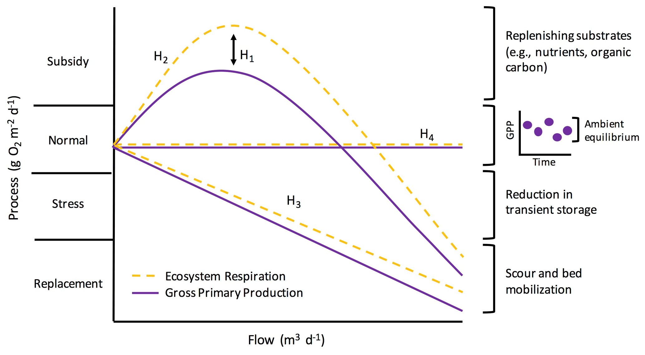
Figure 1 Potential metabolic responses along a subsidy–stress gradient of stream flow (adopted from Odum et al., 1979). Flow is on the x axis. The y axis represents ecosystem metabolism (i.e., gross primary production and ecosystem respiration; GPP and ER), scaled to the same “normal” starting values for comparison, and is broken into four categories as proposed by Odum et al. (1979): (1) subsidy (when flow replenishes carbon and nutrients and metabolism increases), (2) normal (periods of dynamic equilibrium under ambient flow), (3) stress (when ecosystem processes are suppressed by disturbance), and (4) replacement (when there is a severe reduction in metabolism and communities are scoured or replaced). H₁–H₄ labels correspond to different hypotheses about how GPP and ER may respond differently to flow (H₁) and how metabolism might change with flow (H₂–H₄), and they are described further in the main text of the “Introduction”. The inset graph next to the “normal” bracket depicts how ambient process rates are best represented by a dynamic ambient equilibrium rather than a fixed point of stability (sensu Odum et al., 1995).

Stream metabolism is an integrative whole-ecosystem estimate of the carbon fixed and respired by autotrophs and heterotrophs. Metabolism is most commonly estimated via diel changes in dissolved oxygen (Hall and Hotchkiss, 2017): autotrophs produce oxygen during gross primary production (GPP); autotrophs and heterotrophs consume oxygen during respiration, which we refer to as ecosystem respiration (ER) when measured at the whole-reach scale. Together, ER and GPP can elucidate whether a stream is a net producer (autotrophic; GPP > ER) or consumer (heterotrophic; ER > GPP) of carbon. Ecosystem metabolism is coupled with other ecosystem processes (e.g., nitrogen uptake; Hall and Tank, 2003) and is used to monitor stream health (Young et al., 2008; Jankowski et al., 2021), as well as ecosystem responses to disturbance and restoration (e.g., Arroita et al., 2019; Blersch et al., 2019; Palmer and Ruhi, 2019).

Metabolism on any given day is influenced by current and past environmental factors. GPP can increase with light (Mulholland et al., 2001; Roberts and Mulholland, 2007), nutrients (Grimm and Fisher, 1986; Mulholland et al., 2001), temperature (Acuña et al., 2004), and transient storage (Mulholland et al., 2001). ER is controlled by organic carbon availability (e.g., Demars, 2019), as well as the same physicochemical conditions as GPP, and consequently often mirrors GPP (e.g., Roberts et al., 2007; Griffiths et al., 2013; Roley et al., 2014). Antecedent conditions may also play a role in the variability in ecosystem responses to flow (McMillan et al., 2018; Uehlinger and Naegeli, 1998). GPP and ER respond differently to flow disturbances (O'Donnell and Hotchkiss, 2019), likely influenced by where the microbes contributing to GPP and ER reside on or within the heterogeneous stream benthos (e.g., Uehlinger, 2000, 2006). Autotroph reliance on light for energy creates a stream bed commonly dominated by photoautotrophic algal communities and associated heterotrophs. Many heterotrophs, on the other hand, are established within the substrata and hyporheic zone, which can increase resistance and resilience of ER relative to GPP (Uehlinger, 2000; Qasem et al., 2019). Environmental drivers of metabolism fluctuate in response to disturbances (e.g., Uehlinger, 2000) but also vary sub-daily to seasonally, thus inducing temporal variation in GPP and ER during base flows that are best characterized as a pulsing steady state or dynamic equilibrium (e.g., Roberts et al., 2007).

The subsidy–stress relationship between flow and ecosystem function likely induces a range of metabolic responses to and recovery from flow changes (Fig. 1). Both GPP and ER may decline due to disturbance during higher flows (Uehlinger, 2006; Roley et al., 2014; Reisinger et al., 2017); however, flow changes can also stimulate metabolism (Roberts et al., 2007; Demars, 2019). Ultimately, resistance is reflected in the capacity of microbial assemblages to withstand a flow disturbance, with metabolic processes not reduced or stimulated outside of a dynamic ambient equilibrium. Resistance captures the instantaneous response of ecosystem metabolism to a flow disturbance. We can also quantify post-disturbance ecosystem responses by estimating resilience: the time it takes for a process to return to equilibrium following a disturbance (Carpenter et al., 1992). The resilience of ER and GPP following a flow disturbance may take anywhere from days to weeks (e.g., Uehlinger and Naegeli, 1998; Smith and Kaushal, 2015; Reisinger et al., 2017), and it likely varies with season and the magnitude of disturbance (Uehlinger, 2006; Roberts et al., 2007). A flow event of lesser magnitude may yield higher resistance and resilience for both GPP and ER by supplying subsidizing, limiting nutrients and organic matter from the terrestrial landscape without inducing extreme scour. Stream metabolism appears to have low resistance to disturbance but high resilience (Uehlinger and Naegeli, 1998; Reisinger et al., 2017). Understanding how different attributes of flow events (e.g., magnitude, timing) control resistance and recovery trajectories is a critical next step in characterizing metabolic responses to flow changes within and among ecosystems.

We quantified ecosystem resistance and resilience over several years of isolated, higher flow events to examine controls on and patterns of stream metabolic responses to disturbance. We had four hypotheses (Fig. 1): (H₁) ER will be more resistant than GPP to flow disturbances, given the protection of many heterotrophs within the streambed; (H₂) there will be a stimulation of GPP and ER at intermediate flow disturbances due to an influx of limiting carbon and nutrients; (H₃) metabolic resistance and resilience will change with the size of the event, with larger flow disturbances inducing more stress due to enhanced scour; and (H₄) some flow events will not push GPP and ER outside of their ambient dynamic equilibrium. In addition to testing the subsidy–stress hypotheses and differences in how GPP and ER may respond to and recover from higher flow events (Fig. 1), we also analyzed the relationships between environmental variables and metabolic responses, including those prior to flow disturbances that may influence how stream microbial communities respond to flow changes. We predicted recent disturbances might make microbes more vulnerable and less resistant to the next high flow disturbance. We analyzed response and recovery dynamics (i.e., resistance and resilience) relative to a dynamic ambient equilibrium for 15 isolated flow events across 5 years in a flashy urban- and agricultural-influenced stream. Our methods were chosen to address a lingering knowledge gap in our understanding of ecosystem processes, which motivated the three overall objectives of this work: (1) quantify how biological processes (GPP and ER) respond to and recover from discrete higher flow disturbances during storms (Fig. 1, H₂–H₄), (2) test how the response and recovery of GPP and ER differ (Fig. 1, H₁), and (3) identify which environmental drivers best explain metabolic resistance and recovery.

2 Methods

2.1 Study site

Stroubles Creek is a third-order, urban- and agricultural-influenced stream draining a 15 km² sub-watershed of the New River in Southwest Virginia in the United States (Fig. A1; O'Donnell and Hotchkiss, 2019). The mean annual precipitation of Stroubles Creek's catchment is 1006 mm, with more than half (54 %) of that precipitation falling from May to October (PRISM Climate Group, 2013). Annual mean air temperature is 11.3 ^∘C (0.4–22.0 ^∘C monthly mean minimum and maximum; PRISM Climate Group, 2013). The catchment draining into Stroubles Creek at our study location is 85.5 % developed, 11.6 % agriculture (pasture and crops), and 2.9 % forested (Homer et al., 2015). Stroubles Creek has been designated an impaired waterway due to high sediment loading, and it has NO₃ concentrations that typically exceed 1 mg L⁻¹ N-NO₃ (O'Donnell and Hotchkiss, 2019); biological oxygen demand in Stroubles Creek appears to be limited by organic carbon availability more than inorganic nutrients (O'Donnell and Hotchkiss, unpublished data). Our study site is part of the Stream Research, Education, and Management Lab (StREAM Lab, https://www.bse.vt.edu/research/facilities/StREAM_Lab.html, last access: 6 August 2020) and has been monitored by Virginia Tech researchers for over 10 years.

2.2 Sensor data collection

High-temporal-resolution sensor data were collected from 8 January 2013 through 14 April 2018. Dissolved oxygen (DO) (mg L⁻¹), turbidity (nephelometric turbidity unit, NTU), conductivity (ms cm⁻¹), pH, and temperature (^∘C) data were logged at 15 min intervals by an in situ YSI 6920V2 sonde (Hession et al., 2020; O'Donnell and Hotchkiss, 2019). Because a freeze event impaired DO measurements from the YSI sonde, we gap-filled with calibration-checked and comparable data from an adjacent PME miniDOT from 1 September 2017 to 14 April 2018 (Fig. A2 in the Appendix; O'Donnell and Hotchkiss, 2019). We obtained the data needed to model the relative change in light over 24 h (Eq. 1) from a nearby weather station (Fig. A1), which also provided estimates of barometric pressure. A Campbell Scientific CS451 pressure transducer recorded stage measurements every 10 min. Velocity (v) and width (w) measurements were taken over multiple years to create site-specific relationships between stage, velocity, wetted width, and discharge (Q). A stage–discharge relationship was created in 2013 and updated in 2018 to allow for daily estimates of depth (z) from Q=vwz. Sensors were calibrated every 2–4 weeks according to best practice recommendations from the manufacturer (Hession et al., 2020) or, in the case of the PME DO sensor, with Winkler titration checks of our 100 % and 0 % calibration solutions (Hall and Hotchkiss, 2017; O'Donnell and Hotchkiss, 2019).

To remove lower-quality sensor data due to sensor error or periods of low flow, we used data cleaning and quality checks as in O'Donnell and Hotchkiss (2019). Briefly, we excluded values below the 1 % and above the 99 % quantile for physicochemical parameters that were heavily skewed (i.e., turbidity and conductivity). We removed physicochemical values we knew to be unreasonable (e.g., turbidity was cut off at zero). We calculated daily medians of physicochemical parameters for all days that had at least 80 % of measurements over the course of the day after confirming the 80 % cutoff as one that would not bias daily medians from dates without gaps in sensor measurements. Data from lower flow periods when individual sensors may have been out of the water (Hession et al., 2020) were excluded when values were out of range of grab sample calibration checks.

2.3 Estimating ecosystem metabolism

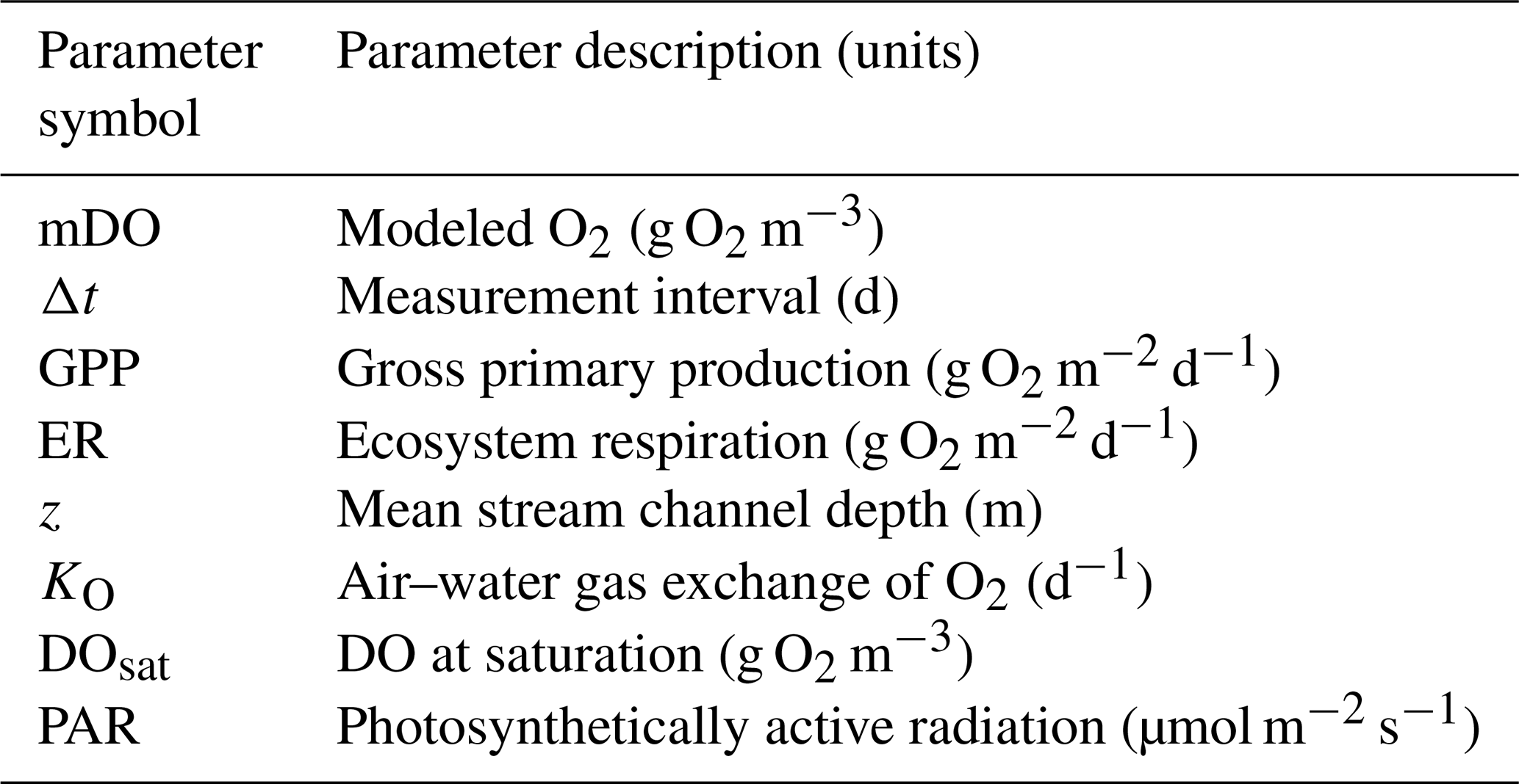
We estimated GPP, ER, and K (the air–water gas exchange coefficient) from diel O₂ (DO), light, and temperature sensor data using the same inverse modeling approach and data as O'Donnell and Hotchkiss (2019). Conservative tracer additions (Hotchkiss and O'Donnell, unpublished data) suggested there are no substantial groundwater inputs to this study reach that would otherwise bias our estimates of GPP and ER (Hall and Hotchkiss, 2017). We selected the streamMetabolizer R package for our analyses (Appling et al., 2018a), which uses Bayesian parameter estimation and a hierarchical state space modeling framework to generate daily estimates of GPP, ER, and K that create the best fit between modeled and observed DO data (Appling et al., 2018b; Eq. 1; Table 1). In Eq. (1), GPP is multiplied by the proportion of modeled light at the previous measurement (PAR_i−Δt) to total daily light (∑PAR) to inversely model diel changes in DO (mDO).

$$\begin{array}{}\text{(1)}& \begin{array}{rl}{\mathrm{mDO}}_i& ={\mathrm{mDO}}_{i-\mathrm{\Delta }t}+{\displaystyle \frac{\mathrm{GPP}\times {\mathrm{PAR}}_{i-\mathrm{\Delta }t}}{z\times \mathrm{\Sigma }\mathrm{PAR}}}+{\displaystyle \frac{\mathrm{ER}}{z}}\mathrm{\Delta }t\\ & +K_{\mathrm{O}}({\mathrm{DO}}_{\mathrm{sat}(i-\mathrm{\Delta }t)}-{\mathrm{mDO}}_{i-\mathrm{\Delta }t})\mathrm{\Delta }t\end{array}\end{array}$$

Table 1 Parameter symbols, descriptions, and units used in Eq. (1).

We modeled GPP, ER, and K with both observation error and process error. We used most of the default model specs for streamMetabolizer. Model convergence was visualized via traceplot in the rstan package (Stan Development Team, 2019) to identify the proper number of burn-in steps (500); we saved 2000 Markov chain Monte Carlo (mcmc) steps from four chains after burn-in. We calculated credible intervals for posterior estimates of GPP and ER derived from the mcmc-derived distributions of GPP and ER. Additionally, to decrease the chances of equifinality between GPP, ER, and K estimates (Appling et al., 2018b), we constrained day-to-day variability in K by binning the range of possible K estimates according to discharge (O'Donnell and Hotchkiss, 2019). We divided yearly discharge into six bins, which the hierarchical modeling framework of streamMetabolizer then used to create K–Q relationships to constrain model K estimates (O'Donnell and Hotchkiss, 2019). We used nighttime linear regression of DO as another way to estimate the range in K in Stroubles (Hall and Hotchkiss, 2017) and used regression-derived estimates of K to quality-check values of modeled K from streamMetabolizer (e.g., Fig. A3). We quality-checked metabolism model output as in O'Donnell and Hotchkiss (2019). We removed all metabolism estimates that were biologically impossible, such as negative GPP or positive ER (ER is modeled as a negative flux of O₂ consumption). Next, we used diagnostics from fit() in stan to remove values resulting from a poor model fit or lack of chain convergence (Stan Development Team, 2019). We removed dates with poor model convergence when Rhat exceeded 1.1 and poor model fit when N_eff (effective sample size) ended at or exceeded the product of the number of chains (4) and the number of saved mcmc steps (2000) specified for our model. Additionally, to avoid using biased estimates of metabolism, we removed days with K values below the 1 % (<3.38 d⁻¹) and above the 99 % (>27.21 d⁻¹) quantile of model estimates. A total of 246 d of metabolism estimates were ultimately removed due to these model output evaluation criteria, resulting in 1375 d (of 1621 total from 8 January 2013 to 14 April 2018) of quality-checked GPP and ER for further analyses.

2.4 Selection of isolated flow events

To identify flow events for our analyses of metabolic resistance and resilience, we calculated the percent change in cumulative daily discharge (Q) relative to the day prior (Eq. 2).

$$\begin{array}{}\text{(2)}& \mathit{\%}\mathrm{\Delta }Q={\displaystyle \frac{Q_i-Q_{i-\mathrm{1}}}{Q_{i-\mathrm{1}}}}\times \mathrm{100},\end{array}$$

where Q_i is the discharge of the day of interest and Q_i−1 is the discharge during the previous day. We selected isolated flow events that had a greater than 50 % Q change relative to the antecedent cumulative daily Q. We defined isolation as a period of 3 d before and 3 d after a high flow event when no other flow events exceeding 10 % Q change occurred. In total, there were 15 isolated flow events across all 5 years that met our criteria for isolated flow events and had quality-checked metabolism estimates (Fig. 2). A hydrograph and metabolism time series plot for each isolated flow event are available in Figs. A4–A18.

Figure 2 (a) Time series of cumulative daily discharge (m³ d⁻¹) on all days with quality-checked metabolism estimates from 8 January 2013 to 14 April 2018. The 15 isolated flow events analyzed for metabolic responses to higher flow are represented by open squares. (b) Frequency distribution of cumulative daily discharge for days with quality-checked metabolism estimates. Vertical dashed lines denote the cumulative daily discharge values of the 15 different isolated flow events. (c) Box plots of cumulative daily discharge for all days with metabolism estimates and those isolated flow event days that fit our criteria for analyzing metabolic resistance and resilience.

The goal of this work was to assess how metabolism responded to and recovered from higher flow events that were also isolated flow events. The designation of 50 % change in flow for high flow events ensured analyzed events were outside of the range of baseline flows. We defined a flow event as >10 % change in Q when comparing the high flow changes to prior metabolic rates as smaller changes in Q may still influence metabolism. In testing different thresholds of flow change and different discharge metrics, we settled on our current method to optimize the thresholds for a change in Q that resulted in the highest number of quality-checked events while ensuring differences between classifications of ambient stream flow and higher flow events. We focused on quality over quantity when selecting for and analyzing stream metabolism results before, during, and after high flow events. To calculate resistance and recovery, we needed consecutive days of high-quality metabolism estimates, which further limited the number of high flow events appropriate for our analyses. For example, in 2016, there were 52 (out of 352) days with quality-checked sensor data that had a 50 % flow change relative to the day prior. After looking at these 52 storms and selecting those that had 3 d before and 3 d after without any other flow events, we had 12 that were isolated. After quality-checking our metabolism estimates for all of those days, we had four high flow events from 2016 that passed all quality-checking steps required for this analysis.

2.5 Characterizing metabolic resistance and resilience

To acknowledge the ambient day-to-day variability in GPP and ER, we used metabolism estimates from 3 d prior to each isolated flow event to calculate a mean value of antecedent metabolism. We quantified metabolic responses to flow disturbances by comparing the pre-event metabolic means with event and post-event metabolism rates. We estimated the metabolic magnitude of departure (M) during events to quantify the resistance of GPP and ER to higher flow disturbances. We calculated M per isolated flow event by comparing the difference between GPP and ER to the mean of the antecedent range (Eq. 3; Fig. 3),

$$\begin{array}{}\text{(3)}& M=\mathrm{1}-{\displaystyle \frac{X_{\mathrm{event}}}{X_{\mathrm{prior}}}},\end{array}$$

where X_event is either GPP or ER (g O₂ m⁻² d⁻¹) on the day of the isolated flow event. X_prior is the mean value of GPP or ER from the antecedent range, and whether M is positive or negative depends on if the isolated flow event resulted in a stimulated (increased) or suppressed (reduced) metabolic response. For instance, if GPP declined during a flow event, M was calculated as the difference between GPP for the isolated flow event and the mean value from the antecedent 3 d range (Fig. 3). A negative M represents a suppression and a positive M a stimulation of GPP or ER relative to the antecedent mean. If GPP or ER on the event day did not fall above or below the antecedent mean, M was zero, thus indicating high resistance.

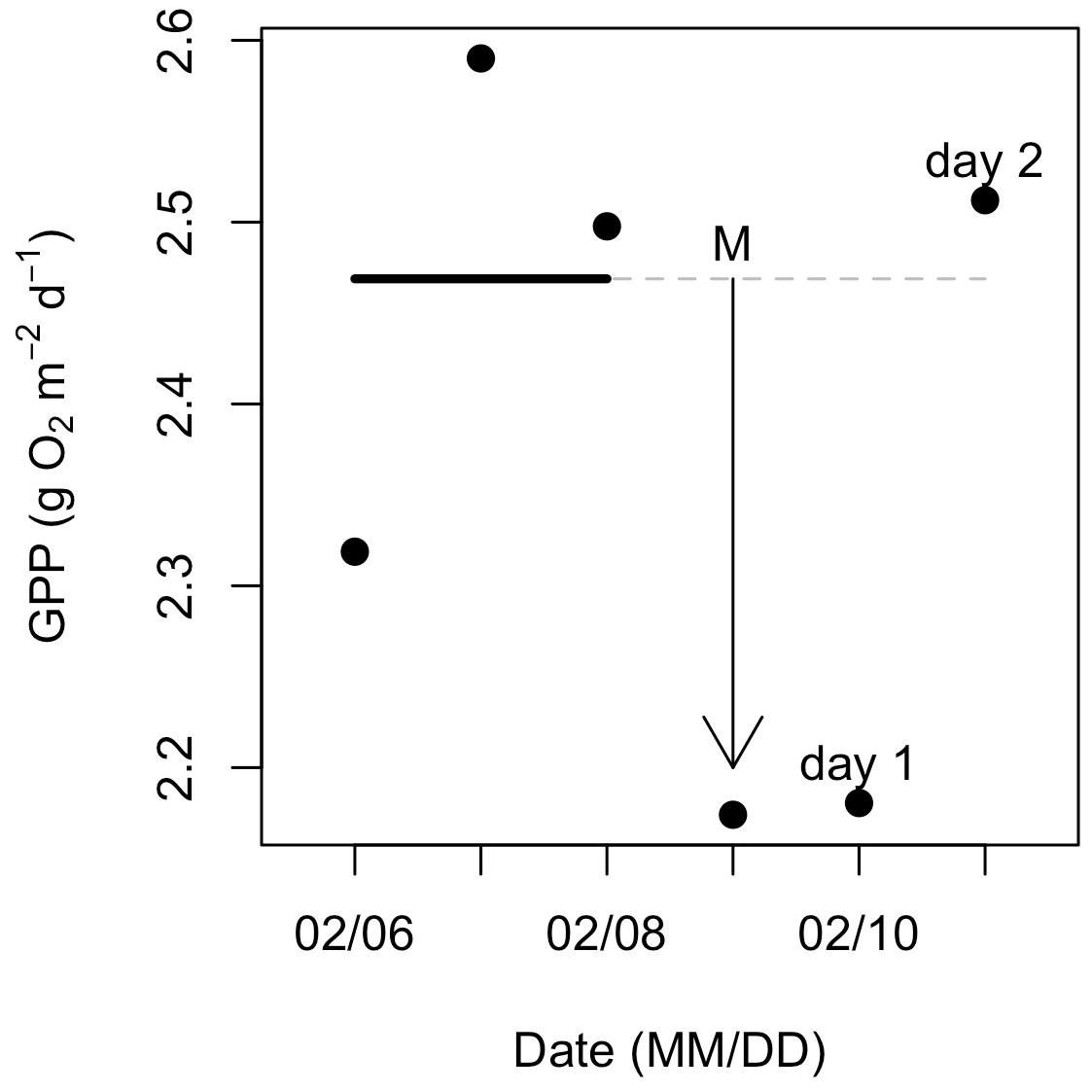
Figure 3 Example calculations of metabolic resistance (magnitude of departure; M) and resilience (recovery interval; RI). Daily gross primary production (GPP) was estimated for the 3 d before, 1 d during, and 2 d following an isolated flow event that occurred on 9 February 2017. The solid (prior to the flow event) and dashed (during and after the flow event) horizontal line represents the mean of GPP estimates from 3 d prior to the flow event. In this case, GPP declined with higher flow, and the magnitude of departure (M with arrow) is the difference between mean prior GPP (dashed line) and GPP during the event. After this flow event, GPP recovered to its prior mean on day two.

To quantify the resilience of GPP and ER, we estimated recovery intervals (RIs) by counting the number of days until metabolic rates returned to or exceeded pre-event mean GPP or ER, signifying a return to antecedent ambient conditions (Fig. 3). If metabolism (mean and 2.5 %–97.5 % credible intervals) during the isolated flow event did not fall outside of the antecedent mean, the RI was 0 d (metabolism cannot recover if it never shifts outside the ambient values). To ensure additional flow events did not obscure the recovery interval of GPP or ER, we stopped counting RI the day before the next event (i.e., if another flow event happened 4 d later, we stopped counting RI at 3 d). To test for statistically significant differences between ER and GPP recovery intervals (RI_ER and RI_GPP) and ER and GPP magnitude of departure (M_ER and M_GPP), we ran Welch's t tests in R (R Core Team, 2018).

While limiting our assessment to isolated flow events decreased the number of suitable events for analysis, our choice of methods allowed us to focus on metabolic response and recovery to discrete disturbances and avoid biased comparisons of multiple high flow (but not isolated) events that encompass time periods long enough (e.g., weeks) for which pre–post comparisons are less meaningful. Because flow was so variable, we chose 3 d to balance best practices from past work on metabolic responses to storms (e.g., 4 d of prior stable baseflow; Reisinger et al., 2017) while ensuring we could analyze as many events with quality-checked data as possible.

2.6 Testing controls on metabolic resistance and resilience

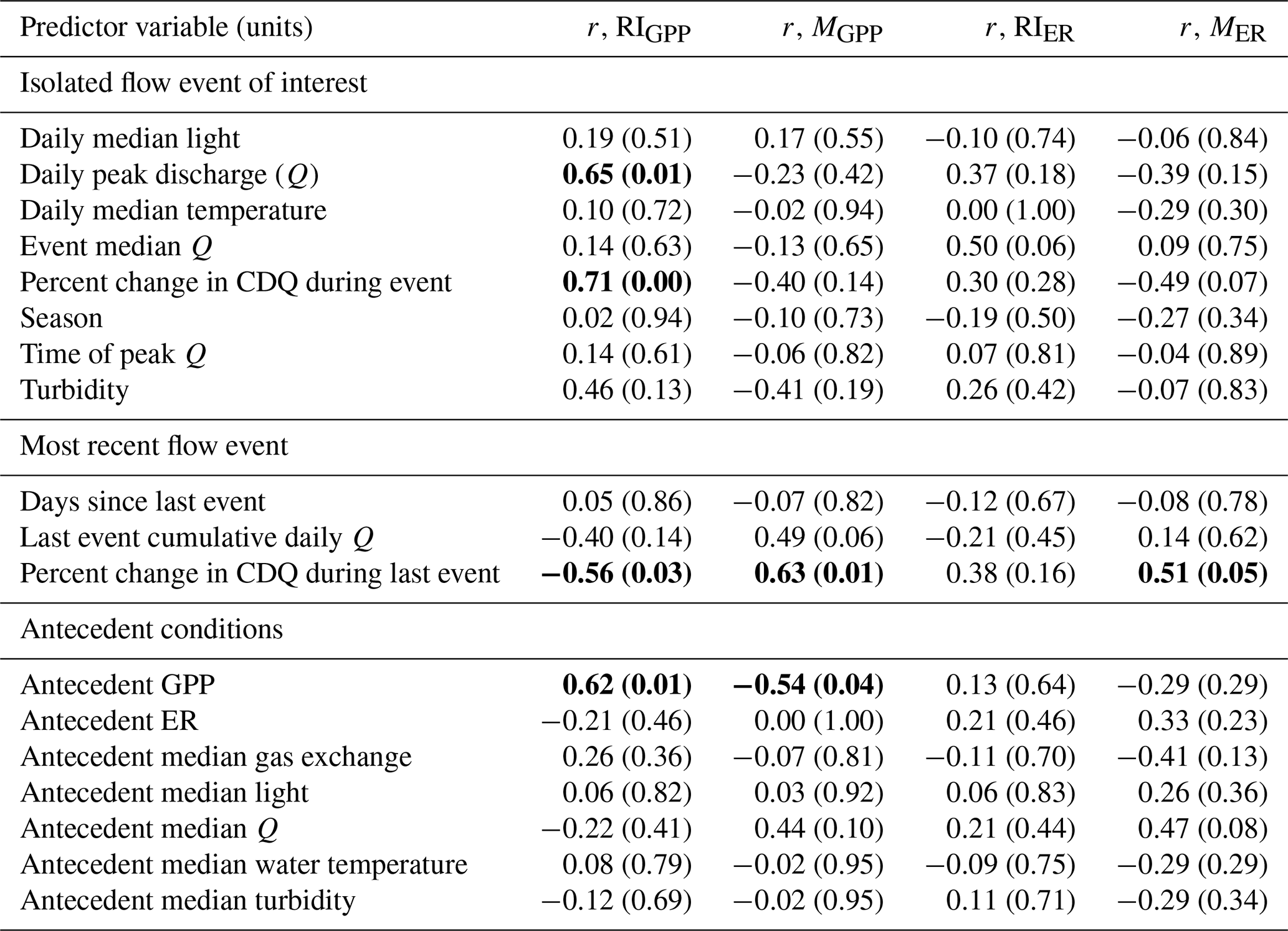
We assessed three categories of potential predictors of metabolic resistance and resilience: antecedent conditions, characteristics of the isolated flow event, and characteristics of the most recent prior flow event. Antecedent conditions included median GPP, ER, turbidity, water temperature, and light. Antecedent medians for turbidity were estimated from 7 d prior due to missing sensor data. We had to remove poor-quality data from the turbidity dataset and chose to set methods that would accommodate inclusion of the most storms for our analysis. We compared the outcome of changing the number of days prior to events with turbidity data available for both 3 and 7 d analyses and found no difference in the results. For all other variables, we estimated values from 3 d prior to the flow event for correlations between metabolism M and RI. Flow event characteristics included flow magnitude (percent change in cumulative daily discharge; Eq. 2), time of peak discharge, and environmental conditions (e.g., light, temperature, turbidity, season) on the event day. Characteristics of the most recent flow event included the magnitude of and days since the last flow event. We visually identified the most recent flow event (percent change in cumulative daily discharge > 50) prior to each isolated flow event. We ran bivariate correlation analyses to quantify the strength and directions of linear relationships between predictor variables and metabolic resistance and resilience using the R cor.test function (R Core Team, 2018). We interpreted correlation strengths as follows: negligible (r = 0.0–0.3), low (0.3–0.5), moderate (0.5–0.7), or high (0.7–1.0) (Hinkle et al., 2003). All modeling and analyses were conducted in R (R Core Team, 2018).

3 Results

3.1 Flow and metabolism

Stroubles Creek is a hydrologically dynamic stream with frequent high flow events (Fig. 2). Cumulative daily discharge for days with quality-checked metabolism estimates ranged from 66 to 114 408 m³ d⁻¹, with a median of 6230 m³ d⁻¹. The 15 isolated flow events selected for analyses were within the mid–high range of all cumulative daily discharge values and were of magnitudes that occurred multiple times a year (Table 2, Fig. 2). We identified isolated flow events of interest based on percent changes in flow, so changes in cumulative daily discharge are proportional across seasons. During the entire measurement period, GPP ranged from 0.00 to 17.3 g O₂ m⁻² d⁻¹ (median = 3.7); ER ranged from −2.2 to −20.5 g O₂ m⁻² d⁻¹ (median = −9.6) (Fig. 4; O'Donnell and Hotchkiss, 2019). Stroubles was heterotrophic ($\left|\mathrm{ER}\right|>\mathrm{GPP}$), except for 38 d (3 %) when GPP > ER, all of which occurred in spring except for 1 d in the fall.

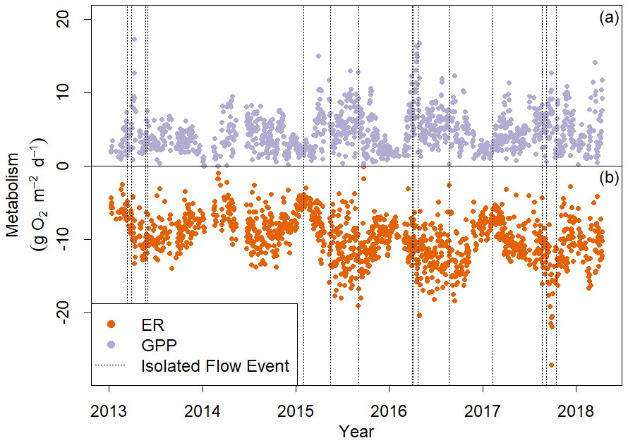
Figure 4 Gross primary production (GPP, a) and ecosystem respiration (ER, b) in Stroubles Creek, VA, from 8 January 2013 to 14 April 2018. ER is represented here as a negative rate because it is the consumption of oxygen. Dashed vertical lines mark the isolated flow events that fit our criteria for analyzing metabolic responses to flow change (Fig. 2).

Table 2 Cumulative daily discharge (CDQ), percent change in CDQ relative to the prior day, metabolism (gross primary production (GPP), ecosystem respiration (ER)), and air–water gas exchange (K) of isolated flow events analyzed for metabolic recovery.

3.2 Metabolic resistance and resilience

GPP most often declined following an isolated flow event (11 of 15 events had suppressed GPP on the high flow day), whereas ER was less likely to deviate from the antecedent equilibrium during higher flows (10 of 15 events had ER credible intervals that overlapped with antecedent mean ER). The magnitude of departure for GPP (M_GPP) ranged from −0.95 to 0.34, with a mean of −0.38 (Table 3; Figs. 5, 6). GPP was inhibited during 11 and slightly stimulated (credible intervals still overlapped prior mean GPP) during 3 of 15 isolated flow events. The magnitude of departure for ER (M_ER) ranged from −0.74 to 0.45, with a mean of −0.09 (Table 3; Figs. 5, 6). ER (mean and credible intervals) did not deviate from the antecedent mean for 10 events (i.e., M_ER was close to zero). ER responses to elevated flow were more variable than those of GPP; ER was both stimulated and suppressed during different high flow periods.

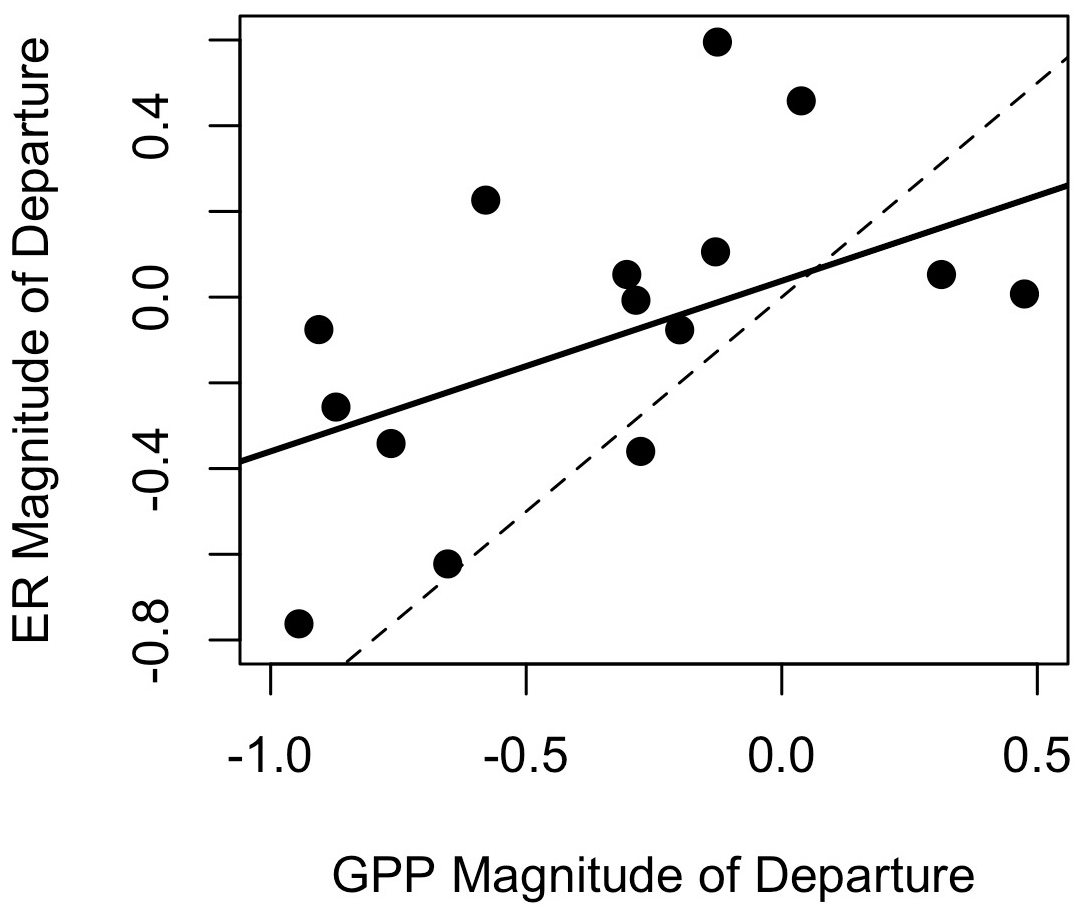
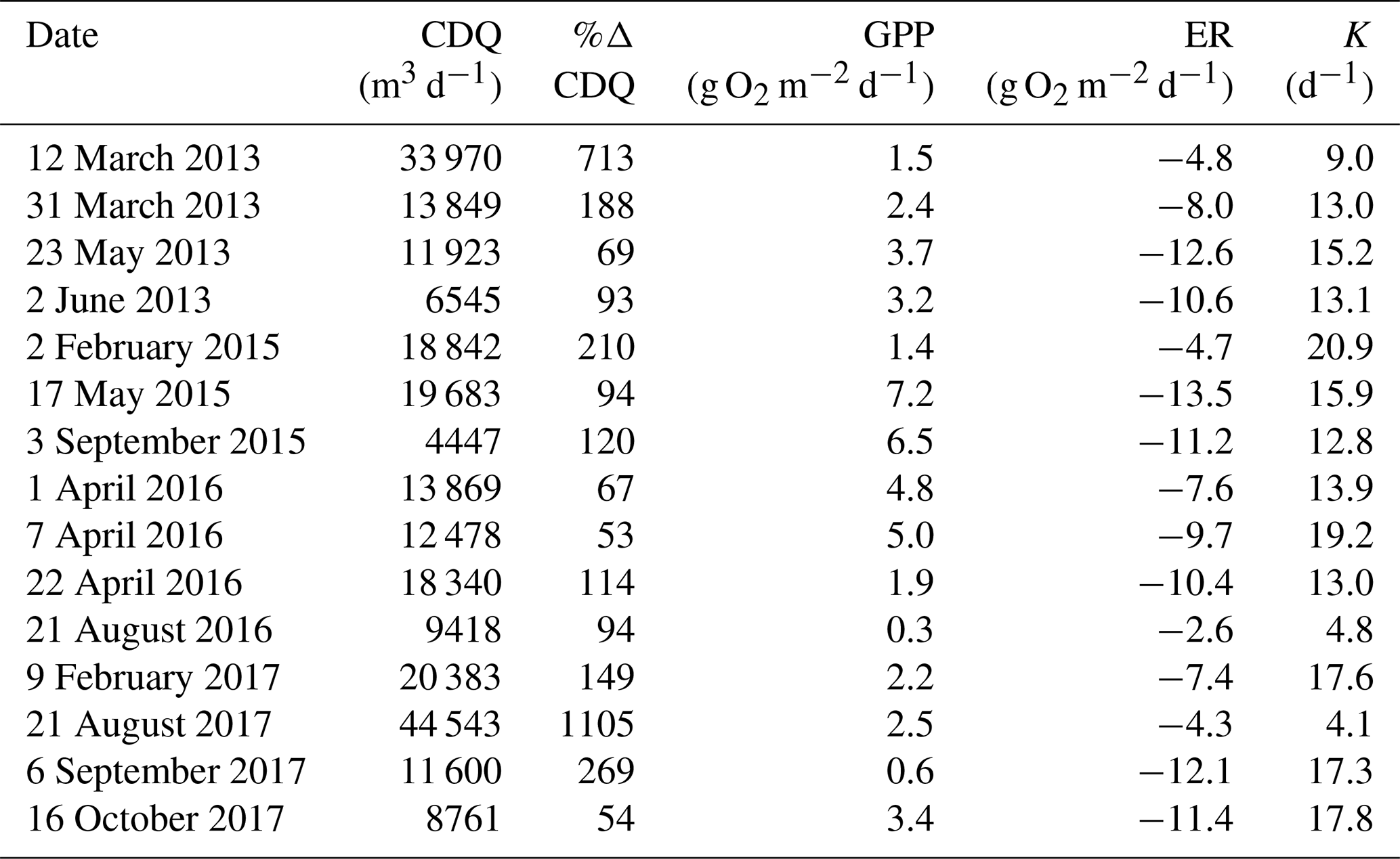
Figure 5 Resistance (i.e., magnitude of departure) of gross primary production (GPP) versus ecosystem respiration (ER) in Stroubles Creek, VA. Dashed line is the 1 : 1 line; solid line is the linear model fit through all data (R²=0.25, p=0.03).

Figure 6 Flow event magnitude (percent change in cumulative daily discharge (Q) relative to the day prior) was negatively correlated with magnitude of departure (M) for gross primary production (GPP; R²=0.10, p=0.143) and ecosystem respiration (ER; R²=0.18, p=0.066). The solid purple line is the regression line for the relationship between M_GPP and percent change in discharge, while the dashed orange line is the regression line for the relationship between M_ER and percent change in discharge.

Table 3 Magnitude of departure (M, unitless) and recovery intervals (RIs, days) of gross primary production (GPP) and ecosystem respiration (ER) during and after 15 isolated flow events between 8 January 2013 and 14 April 2018. A negative M represents a suppression. A positive M is a stimulation, in which GPP or ER increase relative to the prior mean GPP or ER calculated over 3 d. Estimates of M differed between GPP and ER (t(26.3)=2.15, p=0.04), while the RIs for GPP and ER were not significantly different ($t\left(\mathrm{25.8}\right)=-\mathrm{1.22}$, p=0.23). The two instances when GPP did not recover during the isolated flow event analyzed are noted with an “n/a” (not applicable) and the number of days without recovery (X+) that could be counted before the next high flow event occurred.

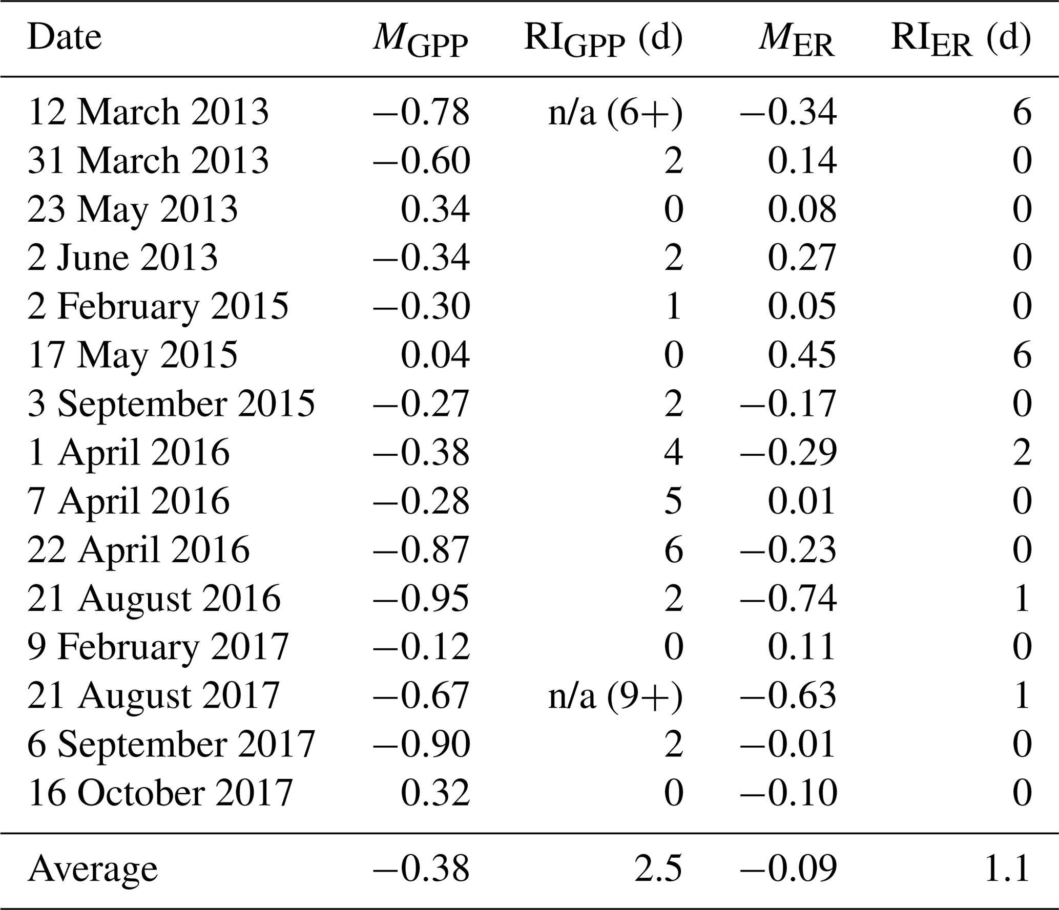
GPP exhibited stronger responses across isolated flow events than ER; M_GPP and M_ER were positively correlated (R²=0.25, p=0.03, Fig. 5) and significantly different (t(26.3)=2.15, p=0.04). M_GPP was lower than M_ER for nearly all flow events, except for three in which M_GPP and M_ER were near zero (Table 3, Figs. 5, 6, A19). The isolated flow event that induced the greatest stimulation of GPP (M_GPP=0.34) also stimulated ER (M_ER=0.08), but the credible intervals of GPP and ER on the high flow day overlapped with prior GPP and ER (Fig. A6). The one flow event that stimulated ER (M_ER=0.45) had a GPP response near zero (M_GPP=0.04). Similarly, the only other event that stimulated GPP (M_GPP=0.34) had a minor ER response (M_ER=0.08), suggesting many flow disturbances may decouple GPP and ER.

Both GPP and ER typically recovered from flow-related stimulation or reduction in less than 3 d (Table 3). There were many isolated flow events when GPP took multiple days to recover, but ER never departed from the antecedent mean (i.e., RI = 0; Fig. 5). When M_GPP and M_ER were both greater than zero, ER almost always recovered faster than GPP. RI_GPP ranged from 0 to 9+ d, with an average of 2.5 d (Table 3). RI_ER ranged from 0–6 d, with an average of 1.1 d (Table 3). There were only two isolated flow events when GPP recovered before ER. While ER always recovered before another flow event occurred, GPP did not recover before another flow event for 2 of 15 analyzed events. The recovery intervals for GPP and ER were not significantly different across all isolated flow events ($t\left(\mathrm{25.8}\right)=-\mathrm{1.22}$, p=0.23).

3.3 Controls on metabolic resistance and resilience after a flow disturbance

Although GPP and ER are linked processes, the variables that were moderate or strong predictors of resistance or resilience (r>0.5) differed between ER and GPP (Table 4). The two predictors with moderate or stronger relationships with both M_GPP and RI_GPP were the percent change in Q during the most recent high flow event and antecedent mean GPP. The percent change in Q during the most recent high flow event was positively correlated with M_ER (r=0.51). The magnitude of each disturbance, characterized by the percent change in cumulative daily discharge, was negatively correlated with M_GPP ($r=-\mathrm{0.40}$, p=0.14) and M_ER ($r=-\mathrm{0.49}$, p=0.07) (Fig. 6) and positively correlated with RI_GPP (r=0.71, p=0.003). Overall, there were multiple environmental controls on metabolic resistance or resilience that had low correlations with either GPP or ER but no significant drivers of both GPP and ER resistance and resilience (Table 4).

Table 4 Pearson correlations (r) between predicted drivers of gross primary production (GPP) and ecosystem respiration (ER) magnitudes of departure (M) and recovery intervals (RIs) of isolated flow events. Predictor variables with moderate or stronger relationships (r>0.5; Hinkle et al., 2003) are bolded. The p values are included in parentheses. CDQ = cumulative daily discharge.

4 Discussion

4.1 Metabolic resistance and resilience

GPP and ER responded differently to flow events in a heterotrophic stream draining an urban–agricultural landscape. Notably, ER was more resistant than GPP to metabolic changes induced by higher flow (Figs. 5, 6). Of the 15 isolated flow events analyzed here, 3 events suppressed ER, and there were 11 instances of GPP suppression (Table 3). Although heterotrophic activity was disturbed by flow changes, 10 of 15 events analyzed in this study had M_ER near zero. Furthermore, a pattern emerged in Stroubles Creek metabolism when analyzed across all flows in a previous study: GPP decreased, but ER was relatively constant on days with higher than median flow (O'Donnell and Hotchkiss, 2019), suggesting a balance between subsidy (e.g., increased inputs of organic carbon from terrestrial sources) and stress buffered changes in ER during higher flows (Roberts et al., 2007; Demars, 2019).

ER was also more resilient than GPP. Differences in ER and GPP resilience were likely a result of flow-induced changes to physicochemical parameters (e.g., increasing turbidity with higher flows) that decrease GPP (O'Donnell and Hotchkiss, 2019). For instance, sustained periods of high turbidity following a flow disturbance can prolong the recovery of GPP by inhibiting light attenuation (Blaszczak et al., 2019). In contrast, higher ER resilience is likely a function of greater resistance of ER to disturbances (i.e., smaller M; Table 3), as well as flow-induced ER stimulation. The correlation of M_GPP and M_ER, but a lack of correlation between RI_GPP and RI_ER (Fig. 5, Table 3), suggests GPP and ER were temporarily decoupled while recovering despite similar initial responses of GPP and ER to flow disturbances.

We do not discuss net ecosystem production results in the context of this work as the patterns mirror those for ER (O'Donnell and Hotchkiss, 2019); however, we note that during the high flows when GPP and ER responses differed, Stroubles Creek was even more heterotrophic due to the higher resistance and resilience of ER relative to GPP. How often and when GPP and ER respond similarly to flow disturbances may differ among ecosystems as a function of their metabolic balance (GPP : ER), nutrient limitation status, and history of flow disturbance. Ultimately, flow-induced changes disproportionately disturbed GPP relative to ER, even in a stream like Stroubles Creek with frequently dynamic flows and relatively short recovery times.

The dynamic nature of stream metabolism, even during low flow periods, must guide how we quantify metabolic responses to disturbance. We estimated resistance as a deviation from an antecedent average (e.g., as in Reisinger et al., 2017; Roley et al., 2014) and leveraged posterior information about our certainty in GPP and ER estimates (i.e., Bayesian credible intervals). Additionally, we assigned RIs of 0 d when the mean and credible intervals of high flow GPP or ER overlapped the mean of GPP or ER from 3 d prior to the high flow event. We thus reduced the potential bias of assuming more discrete differences between day-to-day metabolism estimates that may come with using means or medians instead of the full posterior distributions provided by Bayesian parameter estimation. Without acknowledging the dynamic ambient equilibrium of metabolism in many streams and rivers, we may overestimate disturbances in ecosystem function. In assessing metabolic responses and recovery from smaller flow events relative to dynamic metabolism during ambient flows and acknowledging the uncertainty of metabolism model estimates, we found some of the shortest metabolic recovery intervals recorded in the literature (Fig. 7; Table A1 in the Appendix). Incorporating the dynamic nature of metabolism and standardizing calculations of metabolic recovery dynamics will enable more robust, cross-site comparisons of complex ecosystem response to changes in flow.

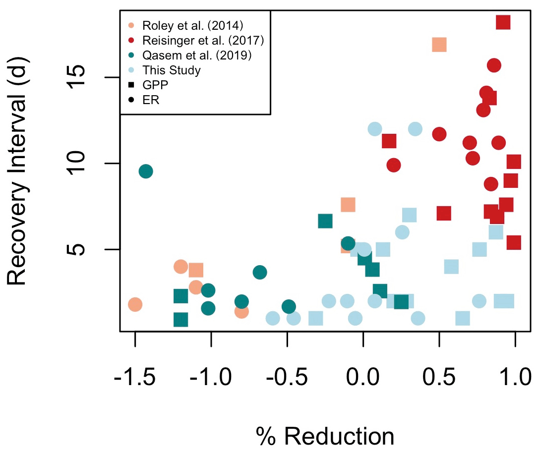
Figure 7 A synthesis of metabolic recovery intervals (days) and percent reduction of gross primary production (GPP) and ecosystem respiration (ER) in response to flow disturbances. A negative percent reduction is a stimulation. Included in Table A1 are additional studies that have reported either recovery intervals or percent metabolic reduction in response to flow disturbances, but not both, and consequently could not be included here.

Our analysis of 15 isolated flow events provided examples of all four hypothesized changes in metabolism with flow (Fig. 1; H₁–H₄). ER was more resistant than GPP to most flow disturbances (H₁). At small-to-intermediate sized flow disturbances, the response of metabolism was variable (H₂, H₃), with the greatest range of metabolic stimulation or reduction (i.e., subsidy or stress) observed at smaller flow changes (Fig. 6). ER and GPP also did not increase or decrease relative to their ambient values during several high flow events (H₄). With increasing intensity of flow disturbance, stress and replacement may indeed scale with intensity (H₃). We note that many smaller streams, even those draining heavily modified landscapes, may continue to play an important role in carbon cycling and nutrient removal, especially during smaller flow disturbances. Further work exploring when and why metabolism–flow dynamics adhere to predicted disturbance responses is critical for a predictive understanding of disturbances, biogeochemical processes, and ecosystem health.

4.2 Controls on metabolic resistance and resilience after a flow disturbance

In addition to testing potential subsidy–stress responses of metabolism to higher flow disturbances, a major objective of this work was to identify controls of metabolic resistance and resilience. While GPP responded similarly to flows regardless of magnitude, ER was more resistant to smaller isolated flow events. Our prediction that isolated flow events of greater magnitudes (i.e., larger percent change in cumulative daily discharge) would result in less resistance and higher M due to increased scouring was supported only marginally for M_GPP and M_ER (Fig. 6, Table 4). GPP appears to have low resistance to flow disturbances, regardless of flow magnitude (Table 4, Fig. 7; Reisinger et al., 2017; Roley et al., 2014). Of the other stream metabolism studies that provided results suitable to be included in our comparison of percent reduction in GPP or ER and metabolic recovery intervals (RI_GPP, RI_ER; Fig. 7), two were from streams draining more heavily urbanized watersheds (Reisinger et al., 2017; Qasem et al., 2019) and one was from a stream draining an agriculturally dominated landscape (Roley et al., 2014). It appears streams draining more urbanized landscapes have higher reductions in metabolism and longer recovery intervals; additional analyses at sites covering a range of land cover types and flow regimes will provide exciting opportunities to see if the trends in Fig. 7 are more broadly applicable.

The different responses of GPP and ER to variable flow may be attributed to differences in energy sources and locations of autotrophs and heterotrophs (Uehlinger, 2000, 2006). Primary producers reside in exposed areas on the streambed to access light required for photosynthesis and are thus more vulnerable to scour than heterotrophic biofilms tucked within, and protected by, substrates in the streambed and hyporheic zone (Uehlinger, 2000). At some threshold of higher flows that disturb more protected areas within and below streambeds, we expect ER will decline as flow-induced stress exceeds flow-induced carbon and nutrient subsidies. Analyses of the interactions between flow-induced changes in shear stress, water depth, and light availability may provide additional insights to tests of potential subsidy–stress dynamics related to stream metabolism. Future analyses that include event duration may also provide new insights into flow–metabolism dynamics: do sustained, higher flows change GPP and ER in the same way as a more instantaneous, intense flow event? As is common with long-term characterizations of metabolism in streams, many high flow days had metabolism model outputs that did not hold up to quality checks and thus were not included in our analyses. Overcoming the logistic and computational challenges of estimating metabolism during extreme flows that disturb deeper substrates will also allow us to better test predictions relating flow magnitude with ecosystem functions.

Quantifying how different antecedent conditions induce variable responses from GPP and ER is critical to furthering our understanding of stream ecosystem responses to flow disturbances. Contrary to our prediction that past scouring might reduce future resistance to disturbances, the size of the most recent antecedent flow disturbance had a positive relationship with both M_GPP and M_ER (Table 4, Fig. A19). M_GPP was smaller and GPP was more resistant when the most recent flow events were larger. Similarly, the percent change in cumulative daily discharge from the last event was positively correlated with M_GPP and M_ER. Stream biota still recovering and regenerating biomass lost from scour might respond differently to flow events depending on the successional stage (Peterson and Stevenson, 1992). Furthermore, biomass growth initially stimulated by a preceding event may have been limited by one or more nutrients later supplied by the isolated flow event. Antecedent GPP and RI_GPP were positively correlated, while M_GPP was negatively correlated with antecedent GPP. We ultimately do not know what caused the negative relationships between the magnitude of the most recent event and M_GPP, as well as M_ER, in Stroubles Creek; quantifying the interactions between recovery of biofilm assemblages and changes in nutrient limitation across multiple flow events may provide greater insights into the mechanisms linking metabolism responses to higher flows with antecedent flow and GPP.

Environmental conditions on the day of isolated flow events that promote biomass growth, such as high light and temperature, were not significant predictors of ER or GPP recovery intervals. Metabolic recovery trajectories often increase with temperature and light (Uehlinger and Naegeli, 1998; Uehlinger, 2000) and consequently may change seasonally, with faster recoveries in spring and slower recoveries in winter (Uehlinger, 2000, 2006). While we did not find strong predictors of RI_ER among the environmental variables in our dataset, changes in the source, magnitude, and biological reactivity of organic matter inputs may alter RI_ER (Roberts et al., 2007). Combining high-frequency nutrient and organic matter quality measurements with metabolic resistance and resilience estimates will offer an improved understanding of how changing nutrients and organic matter mediate metabolic responses to flow changes.

5 Conclusions

Metabolic regimes are punctuated by high flow events that create frequent pulses of stimulated or reduced GPP or ER (e.g., Uehlinger, 2006; Beaulieu et al., 2013; Bernhardt et al., 2018). As such, changes in flow play an influential role in the trends and variability in metabolism. While geomorphology and disturbance regimes may control metabolic resistance across sites (Uehlinger, 2000; Blaszczak et al., 2019), within-site variability in M and RI may be controlled by the characteristics of each flow event, as well as prior flow disturbances. Differences between ER and GPP response and recovery to flow disturbances at our study site were controlled by the higher resistance and resilience of ER relative to GPP. Within this study, our prediction that ER would be more resistant than GPP to flow disturbances was supported as ER frequently did not even deviate from the antecedent ambient equilibrium. However, ER had less resistance to events of greater magnitude. Indeed, both M_ER and M_GPP were negatively correlated with the percent change in discharge of flow event, but M_ER had a stronger negative relationship with the percent change in discharge than M_GPP. Metabolic responses to small and intermediate flow disturbances were variable: GPP and ER were both stimulated and suppressed. We suggest there may be a resistance threshold to flow disturbances, in which controls other than flow magnitude (e.g., season, light, turbidity) might regulate metabolic responses to lower flow changes. Using segmented process–discharge relationships to quantify a resistance threshold of processes to flow disturbances (O'Donnell and Hotchkiss, 2019) may support a more predictive understanding of metabolic response to flow disturbances as it provided insights on how patterns of water-quality parameters and metabolism changed across the full range of flow, thus supporting the inferences we were able to make from storm-specific analyses in this paper.

One motivation of our work was to better understand metabolic dynamics in less pristine ecosystems. Dynamic hydrology makes estimating metabolism more challenging and consequently decreased the number of events with appropriate data for our analysis. Although we analyzed only 15 high flow events in this study, many of the past analyses on related topics included a similar or lower number of events over a shorter time period. Our work fills in substantial knowledge gaps: we analyzed across seasons (not only summer months or a short sensor deployment period) and high flow magnitudes (not only base flow or the highest flow disturbances), which allowed us to show a suite of different metabolic responses to changing flow. We are also left with questions about how ecosystem processes respond to discrete changes: how might environmental drivers of metabolic subsidy or stress determine thresholds of resistance and timelines of recovery? How do recent high flow events facilitate improved resistance to flow disturbances? What is the role of flow duration in altering metabolism within and after high flow events? Ultimately, we are entering an era of metabolic data opportunity (e.g., Bernhardt et al., 2018). As time series of metabolism lengthen and modeling tools improve, we envision exciting opportunities to better assess the consequences of isolated flow events, as well as the impacts of multiple, sequential high flow disturbances that did not meet our criteria for analyzing isolated flow events in this paper. While the short periods between high flow events in many streams and rivers make isolating and quantifying functional resistance and resilience an ongoing challenge, including dynamic flow in our assessment of metabolic regimes is a critical next step toward a more holistic understanding of frequently disturbed ecosystems.

Appendix A

Figure A1 Stroubles Creek watershed and land cover types in the area that drains to the StREAM Lab monitoring site at Bridge 1, Blacksburg, VA, USA (coordinates in decimal degrees: 37.21013, −80.44511). The nearby weather station that provided light and barometric pressure is just west of the watershed boundary and within the same valley. We created this map using ArcGIS, NHDplus version 2.1, and the US Geological Survey's 2011 National Land Cover Database.

Figure A2 Dissolved oxygen measurements from the two sensors – YSI Sonde and PME miniDOT – at Bridge 1 on Stroubles Creek. The spread of YSI Sonde values spanning from the end of January to mid-April was likely a result of a freeze event. We used PME data during the period of record when YSI data did not pass our quality assurance checks. Date format is month/year.

Figure A3 Example of data used to confirm modeled K₆₀₀ (d⁻¹) using a regression of the nighttime dissolved oxygen saturation deficit versus changes in saturation (as in Hall and Hotchkiss, 2017). These data are from 4 September 2017, when the estimated value for K₆₀₀ was 22 d⁻¹.

Figure A4 Cumulative daily discharge and metabolism (gross primary production and ecosystem respiration; GPP and ER) time series for the Stroubles Creek flow event on 12 March 2013 (noted with a dashed vertical red line in all three panels). The dashed horizontal black lines are mean values of GPP and ER prior to the high flow event. Error bars for posterior estimates of GPP and ER are 2.5 % and 97.5 % Bayesian credible intervals.

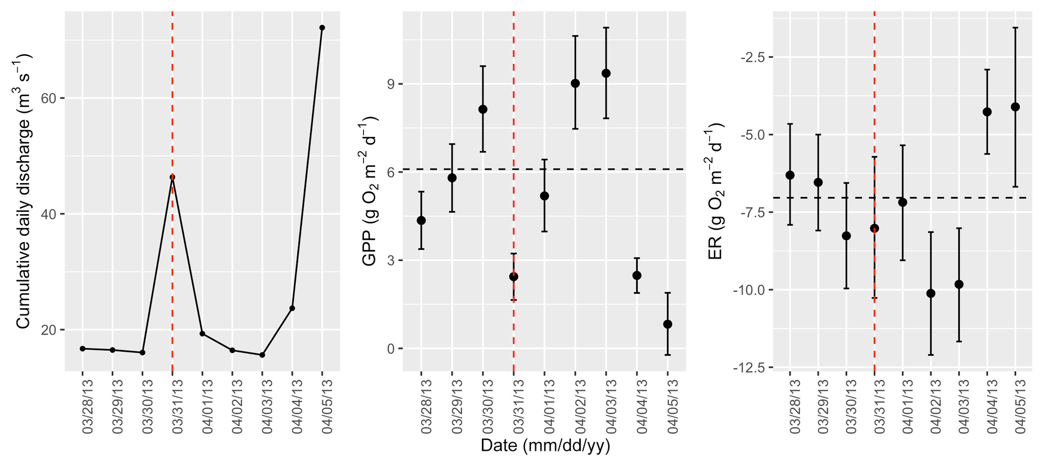
Figure A5 Cumulative daily discharge and metabolism (gross primary production and ecosystem respiration; GPP and ER) time series for the Stroubles Creek flow event on 31 March 2013 (noted with a dashed vertical red line in all three panels). The dashed horizontal black lines are mean values of GPP and ER prior to the high flow event. Error bars for posterior estimates of GPP and ER are 2.5 % and 97.5 % Bayesian credible intervals.

Figure A6 Cumulative daily discharge and metabolism (gross primary production and ecosystem respiration; GPP and ER) time series for the Stroubles Creek flow event on 23 May 2013 (noted with a dashed vertical red line in all three panels). The dashed horizontal black lines are mean values of GPP and ER prior to the high flow event. Error bars for posterior estimates of GPP and ER are 2.5 % and 97.5 % Bayesian credible intervals.

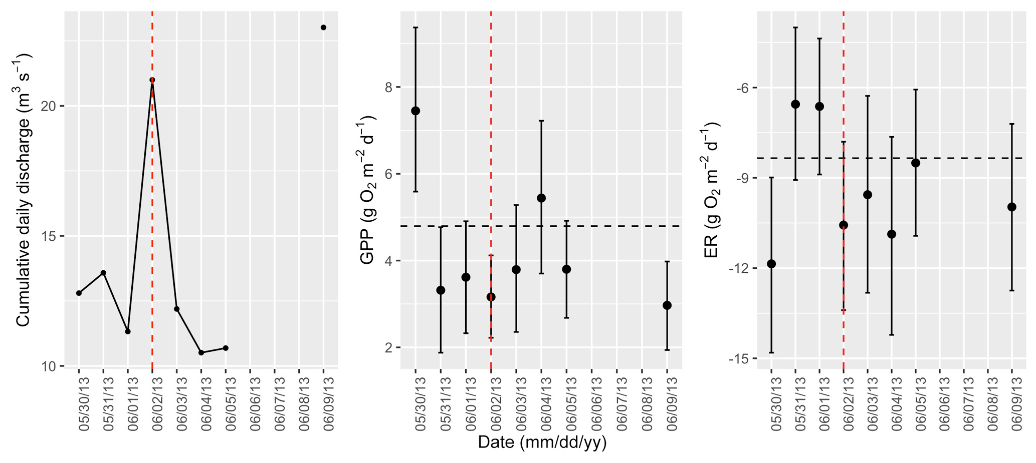
Figure A7 Cumulative daily discharge and metabolism (gross primary production and ecosystem respiration; GPP and ER) time series for the Stroubles Creek flow event on 2 June 2013 (noted with a dashed vertical red line in all three panels). The dashed horizontal black lines are mean values of GPP and ER prior to the high flow event. Error bars for posterior estimates of GPP and ER are 2.5 % and 97.5 % Bayesian credible intervals.

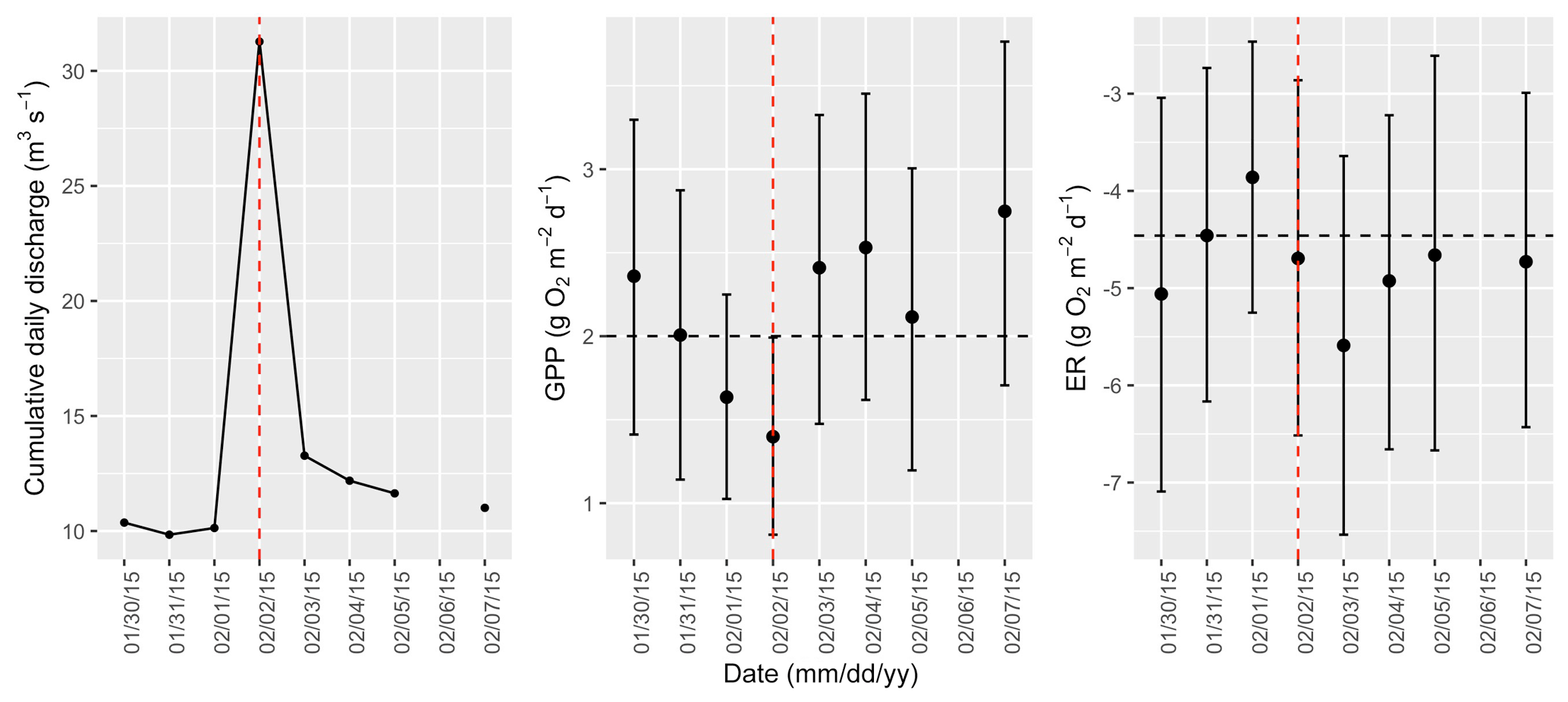
Figure A8 Cumulative daily discharge and metabolism (gross primary production and ecosystem respiration; GPP and ER) time series for the Stroubles Creek flow event on 2 February 2015 (noted with a dashed vertical red line in all three panels). The dashed horizontal black lines are mean values of GPP and ER prior to the high flow event. Error bars for posterior estimates of GPP and ER are 2.5 % and 97.5 % Bayesian credible intervals.

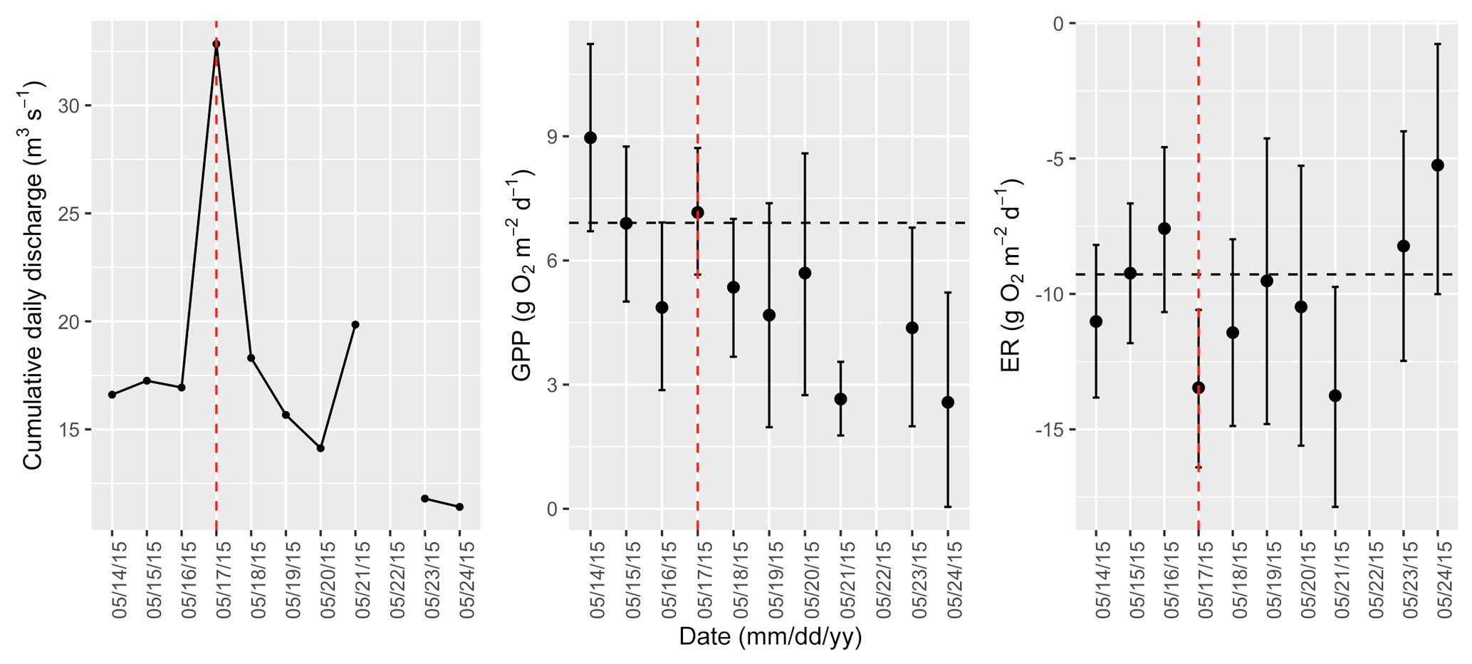
Figure A9 Cumulative daily discharge and metabolism (gross primary production and ecosystem respiration; GPP and ER) time series for the Stroubles Creek flow event on 17 May 2015 (noted with a dashed vertical red line in all three panels). The dashed horizontal black lines are mean values of GPP and ER prior to the high flow event. Error bars for posterior estimates of GPP and ER are 2.5 % and 97.5 % Bayesian credible intervals.

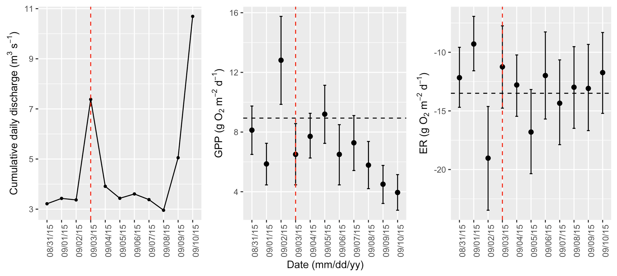
Figure A10 Cumulative daily discharge and metabolism (gross primary production and ecosystem respiration; GPP and ER) time series for the Stroubles Creek flow event on 3 September 2015 (noted with a dashed vertical red line in all three panels). The dashed horizontal black lines are mean values of GPP and ER prior to the high flow event. Error bars for posterior estimates of GPP and ER are 2.5 % and 97.5 % Bayesian credible intervals.

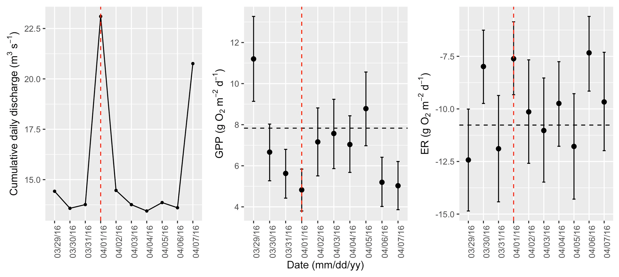
Figure A11 Cumulative daily discharge and metabolism (gross primary production and ecosystem respiration; GPP and ER) time series for the Stroubles Creek flow event on 1 April 2016 (noted with a dashed vertical red line in all three panels). The dashed horizontal black lines are mean values of GPP and ER prior to the high flow event. Error bars for posterior estimates of GPP and ER are 2.5 % and 97.5 % Bayesian credible intervals.

Figure A12 Cumulative daily discharge and metabolism (gross primary production and ecosystem respiration; GPP and ER) time series for the Stroubles Creek flow event on 7 April 2016 (noted with a dashed vertical red line in all three panels). The dashed horizontal black lines are mean values of GPP and ER prior to the high flow event. Error bars for posterior estimates of GPP and ER are 2.5 % and 97.5 % Bayesian credible intervals.

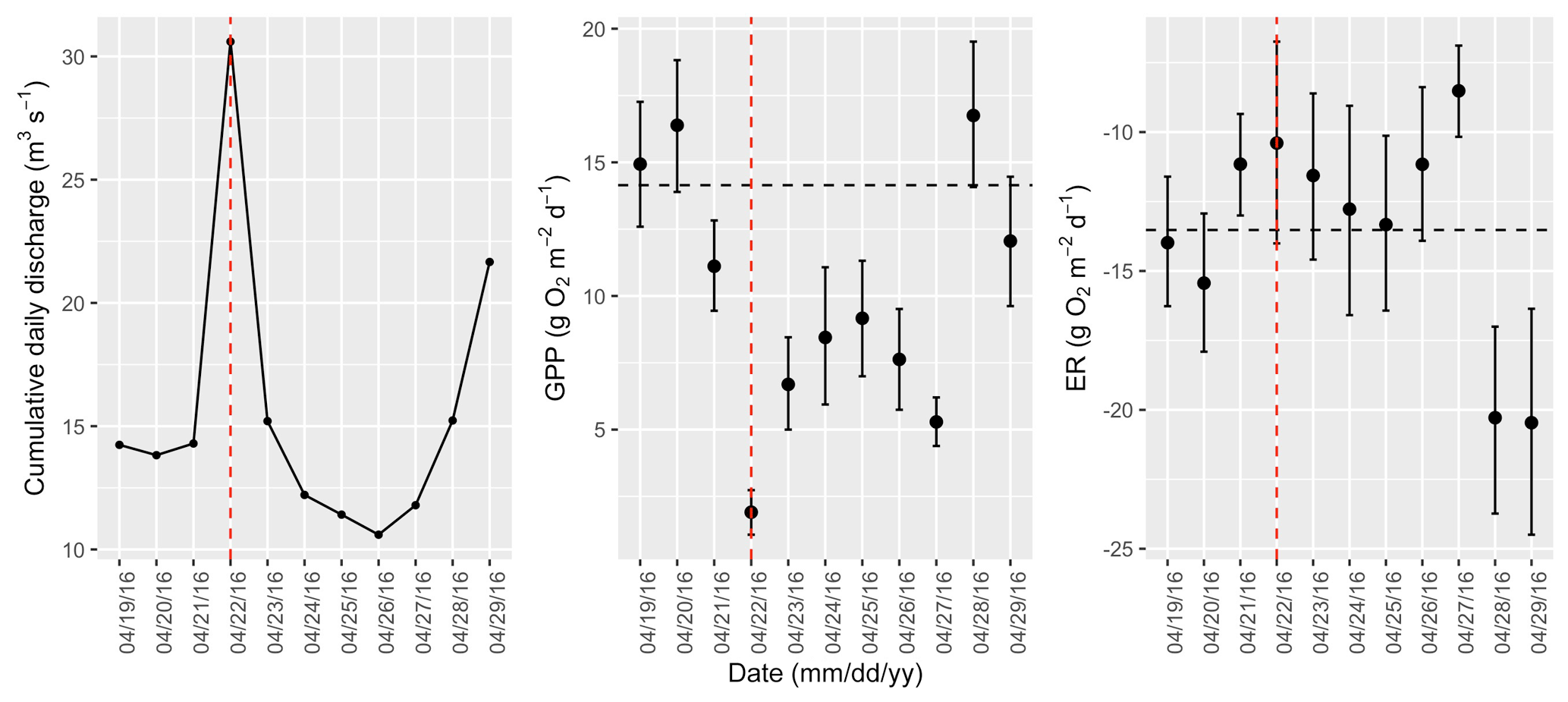
Figure A13 Cumulative daily discharge and metabolism (gross primary production and ecosystem respiration; GPP and ER) time series for the Stroubles Creek flow event on 22 April 2016 (noted with a dashed vertical red line in all three panels). The dashed horizontal black lines are mean values of GPP and ER prior to the high flow event. Error bars for posterior estimates of GPP and ER are 2.5 % and 97.5 % Bayesian credible intervals.

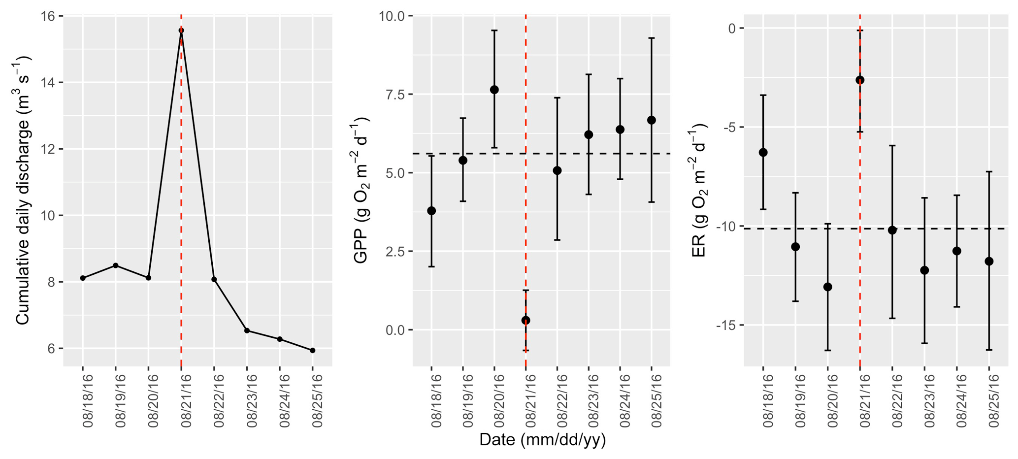
Figure A14 Cumulative daily discharge and metabolism (gross primary production and ecosystem respiration; GPP and ER) time series for the Stroubles Creek flow event on 21 August 2016 (noted with a dashed vertical red line in all three panels). The dashed horizontal black lines are mean values of GPP and ER prior to the high flow event. Error bars for posterior estimates of GPP and ER are 2.5 % and 97.5 % Bayesian credible intervals.

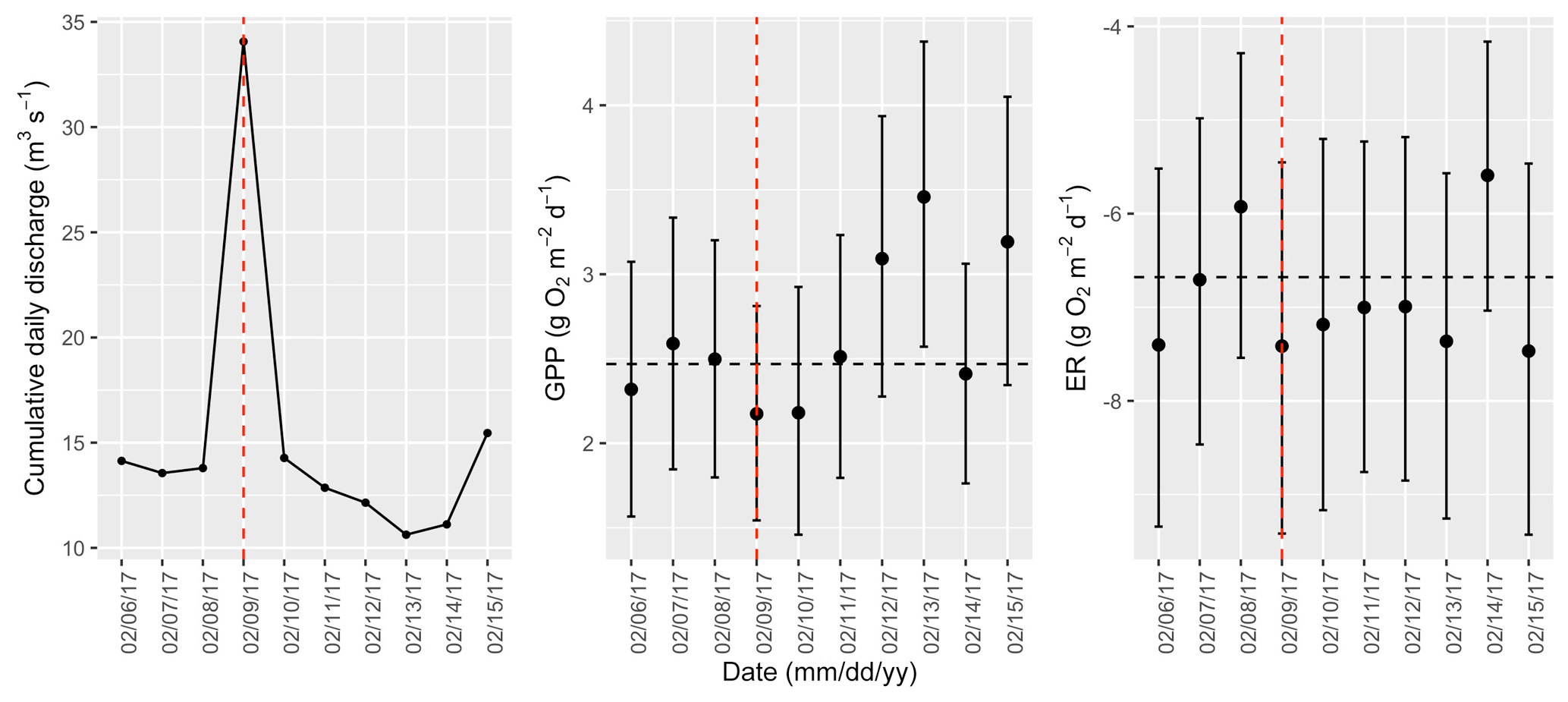
Figure A15 Cumulative daily discharge and metabolism (gross primary production and ecosystem respiration; GPP and ER) time series for the Stroubles Creek flow event on 9 February 2017 (noted with a dashed vertical red line in all three panels). The dashed horizontal black lines are mean values of GPP and ER prior to the high flow event. Error bars for posterior estimates of GPP and ER are 2.5 % and 97.5 % Bayesian credible intervals.

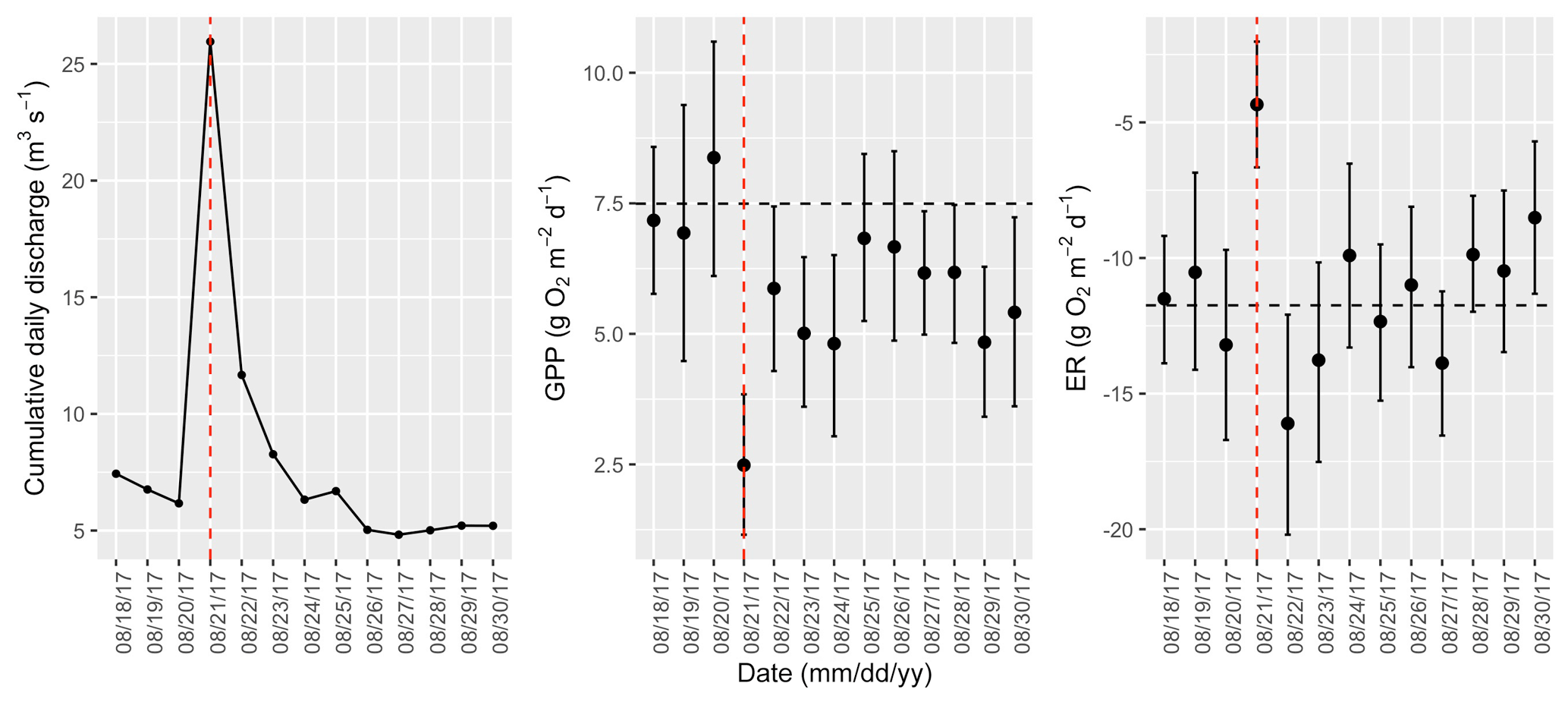
Figure A16 Cumulative daily discharge and metabolism (gross primary production and ecosystem respiration; GPP and ER) time series for the Stroubles Creek flow event on 21 August 2017 (noted with a dashed vertical red line in all three panels). The dashed horizontal black lines are mean values of GPP and ER prior to the high flow event. Error bars for posterior estimates of GPP and ER are 2.5 % and 97.5 % Bayesian credible intervals.

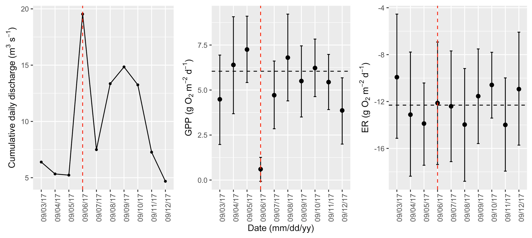
Figure A17 Cumulative daily discharge and metabolism (gross primary production and ecosystem respiration; GPP and ER) time series for the Stroubles Creek flow event on 6 September 2017 (noted with a dashed vertical red line in all three panels). The dashed horizontal black lines are mean values of GPP and ER prior to the high flow event. Error bars for posterior estimates of GPP and ER are 2.5 % and 97.5 % Bayesian credible intervals.

Figure A18 Cumulative daily discharge and metabolism (gross primary production and ecosystem respiration; GPP and ER) time series for the Stroubles Creek flow event on 16 October 2017 (noted with a dashed vertical red line in all three panels). The dashed horizontal black lines are mean values of GPP and ER prior to the high flow event. Error bars for posterior estimates of GPP and ER are 2.5 % and 97.5 % Bayesian credible intervals.

Figure A19 The magnitude of the previous high flow event (percent change in cumulative daily discharge) had a positive relationship with M_GPP and M_ER. GPP is represented by purple squares, and the orange circles are ER. The solid purple regression line reflects the relationship between magnitude of the last event and M_GPP, whereas the dashed orange regression line represents the relationship between the magnitude of the last event and M_ER.

Uehlinger and Naegeli (1998)Uehlinger (2000)Uehlinger (2000)Uehlinger (2006)Roberts et al. (2007)Roberts et al. (2007)Roley et al. (2014)Roley et al. (2014)Roley et al. (2014)Roley et al. (2014)Smith and Kaushal (2015)Reisinger et al. (2017)Reisinger et al. (2017)Reisinger et al. (2017)Reisinger et al. (2017)Reisinger et al. (2017)Reisinger et al. (2017)Reisinger et al. (2017)Reisinger et al. (2017)Reisinger et al. (2017)Reisinger et al. (2017)Reisinger et al. (2017)Qasem et al. (2019)Qasem et al. (2019)Qasem et al. (2019)Qasem et al. (2019)Qasem et al. (2019)Qasem et al. (2019)

Table A1 Literature review of published reduction and recovery intervals (RIs) of stream gross primary production (GPP) and ecosystem respiration (ER) after high flow events. If not enough information was given to calculate reduction or RI, we listed it as “n/a”.

^a Approximated days of recovery from figure in publication. ^b Approximation given in publication.