Tidal mixing of estuarine and coastal waters in the western English Channel is a control on spatial and temporal variability in seawater CO₂

Surface ocean carbon dioxide (CO₂) measurements are used to compute the oceanic air–sea CO₂ flux. The CO₂ flux component from rivers and estuaries is uncertain due to the high spatial and seasonal heterogeneity of CO₂ in coastal waters. Existing high-quality CO₂ instrumentation predominantly utilises showerhead and percolating style equilibrators optimised for open-ocean observations. The intervals between measurements made with such instrumentation make it difficult to resolve the fine-scale spatial variability of surface water CO₂ at timescales relevant to the high frequency variability in estuarine and coastal environments. Here we present a novel dataset with unprecedented frequency and spatial resolution transects made at the Western Channel Observatory in the south-west of the UK from June to September 2016, using a fast-response seawater CO₂ system. Novel observations were made along the estuarine–coastal continuum at different stages of the tide and reveal distinct spatial patterns in the surface water CO₂ fugacity (fCO₂) at different stages of the tidal cycle. Changes in salinity and fCO₂ were closely correlated at all stages of the tidal cycle and suggest that the mixing of oceanic and riverine endmembers partially determines the variations in fCO₂. The correlation between salinity and fCO₂ was different in Cawsand Bay, which could be due to enhanced gas exchange or to enhanced biological activity in the region. The observations demonstrate the complex dynamics determining spatial and temporal patterns of salinity and fCO₂ in the region. Spatial variations in observed surface salinity were used to validate the output of a regional high-resolution hydrodynamic model. The model enables a novel estimate of the air–sea CO₂ flux in the estuarine–coastal zone. Air–sea CO₂ flux variability in the estuarine–coastal boundary region is influenced by the state of the tide because of strong CO₂ outgassing from the river plume. The observations and model output demonstrate that undersampling the complex tidal and mixing processes characteristic of estuarine and coastal environment biases quantification of air–sea CO₂ fluxes in coastal waters. The results provide a mechanism to support critical national and regional policy implementation by reducing uncertainty in carbon budgets.

1 Introduction

The ocean has taken up about a quarter of anthropogenic carbon dioxide (CO₂) emissions to date, absorbing approximately 2.5 Pg C yr⁻¹ (Friedlingstein et al., 2019). Global observations of the partial pressure of CO₂ in seawater (pCO₂) are stored in the Surface Ocean CO₂ Atlas (SOCAT) (https://www.socat.info/, last access: 20 March 2022) (Bakker et al., 2016). The latest version of SOCAT (v2021) contains ∼ 32.7 million pCO₂ measurements, with the majority (≳  75 %) of data collected in the open ocean (Laruelle et al., 2018). The carbon cycle in continental shelf waters has been extensively studied in recent years (Laruelle et al., 2018; Robbins et al., 2018; Kahl et al., 2017; Ahmed and Else, 2019; Laruelle et al., 2017b; Kitidis et al., 2019; Fennel et al., 2019). Whilst the surface area of coastal, estuarine and continental shelf waters makes up 7.5 % of global waters (∼ 2.7 × 10⁷ km²) (Cai, 2011), continental shelves alone have been shown to take up a substantial proportion 0.20–0.25 Pg C yr⁻¹ (8 %–10 %) of global ocean uptake (Laruelle et al., 2018, 2014; Chen et al., 2013; Cai, 2011; Bauer et al., 2013). Estuaries are net heterotrophic and thus typically oversaturated with pCO₂ with respect to the atmosphere (Laruelle et al., 2017a; Frankignoulle et al., 1998). The global air–water CO₂ flux from estuaries is thus into the atmosphere, and this flux is currently perceived to roughly offset the CO₂ uptake by the continental shelves (Cai, 2011; Borges et al., 2006). However, the global estuarine air–water CO₂ flux remains highly uncertain, with estimates ranging from 0.09 to 0.78 Pg C yr⁻¹ (Cai, 2011; Laruelle et al., 2010; Chen and Borges, 2009; Chen et al., 2013; Resplandy et al., 2018; Roobaert et al., 2019).

Estuaries and rivers around major ports and harbours are deep and easily accessed with large research vessels. However, many estuaries are shallow and/or have irregular topography. Navigating shallow estuaries safely, particularly at low tide, is not always possible for many ocean-going research vessels, such that mapping the pCO₂ is challenging. The observations of pCO₂ included in SOCAT from upper estuarine waters come from a limited number of research vessels that are typically small (∼ 25 m long) and have shallow (∼ 3 m) draughts. Transects of large rivers and estuaries by shallow-bottom boats identify a CO₂ concentration gradient between the mouth and source, with high pCO₂ (∼ 10 000 ppm) upriver and pCO₂ levels similar to seawater close to the river mouth (Borges et al., 2018; Joesoef et al., 2015; Macklin et al., 2014; Bozec et al., 2012; Volta et al., 2016; Cai, 2011; Jeffrey et al., 2018b). Assessment of pCO₂ in inland waters, determined from measurements of total alkalinity (TA) and dissolved inorganic carbon (DIC), is also highly uncertain due to limited carbonate buffering capacity at low pH and because acids in terrestrial organic matter make an unknown contribution to the TA anions (Abril et al., 2015).

The zone where estuarine waters meet coastal waters is a physically dynamic system influenced by riverine outflow, winds, waves and tidal cycles; hence, pCO₂ is likely to vary where estuarine water and continental shelf water interact, yet there has been relatively little attention given to air–water CO₂ fluxes in this zone (Cai, 2011). Increased research effort over the past decade has shown that many processes are important in this zone (Cai et al., 2021; Ward et al., 2017; Shen et al., 2019). One holistic modelling study has tried to understand the coastal system in eastern North America, encompassing tidal wetlands, estuaries and continental shelves (Najjar et al., 2018). The study demonstrated that, despite estuaries representing < 10 % of the domain area, interactions with shelf seas must be considered as the estuarine waters gave off more CO₂ than the shelves drew down. Eulerian studies in the estuarine zone have identified large tidal signals in pCO₂ with data collected from research vessels (Borges and Frankignoulle, 1999; Jeffrey et al., 2018a) and from moorings or fixed sites (Dai et al., 2009; Jeffrey et al., 2018a; Li et al., 2018; Bakker et al., 1996; Call et al., 2015; Ferrón et al., 2007; Santos et al., 2012). pCO₂ levels at the mouth of different rivers have been observed to co-vary with changes in river flow rate and with the tidal cycle (Ribas-Ribas et al., 2013; Canning et al., 2021; Najjar et al., 2018; Frankignoulle et al., 1996). Underway CO₂ measurements along transects have been made (Hales et al., 2005) but have not been regularly repeated through the transitional zone where estuaries connect with continental shelf waters.

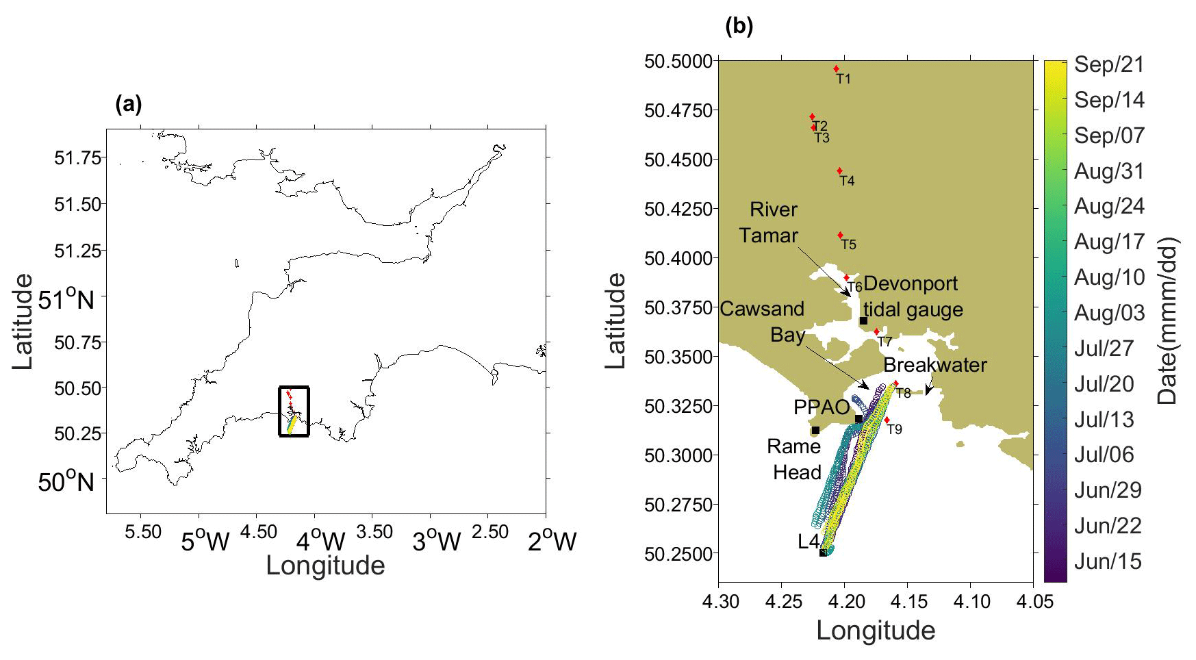
Figure 1 (a) Map of the south-west of the England Western Channel Observatory (WCO) and study area (black rectangle). (b) Breakwater to L4 transects for the 15 transects made with the RV Plymouth Quest (coloured circles). Ship tracks are coloured by date between 10 June and 21 September 2016. The River Tamar, Devonport tidal gauge station, Plymouth Breakwater, Cawsand Bay, PPAO, Rame Head and station L4 are marked. Transect sites T1–T9 are shown as red diamonds.

Here we present weekly surface water fCO₂ observations along a < 8 km transect from estuarine waters into continental shelf waters in the western English Channel between April and September 2016 (Fig. 1). The CO₂ measurement system was capable of high spatial (∼ 0.2 km) and temporal resolution (∼ 48 s), revealing substantial variations in surface fCO₂. Our aim was to examine in detail the transition zone between rivers, estuaries and the coastal zone in order to investigate variations in surface CO₂ and potential drivers of this variation. We then used the observed relationship in the CO₂ and salinity data together with the output of a high-resolution hydrodynamic model of the estuary and nearshore region to estimate the spatial heterogeneity in fCO₂ and air–water CO₂ flux.

2 Study location and physical setting

This study was conducted in the English Channel off the coast of Plymouth (south-west UK) at the Western Channel Observatory (WCO, see Fig. 1a), which includes the oceanographic station L4 (50.251^∘ N, 4.221^∘ W; Smyth et al., 2010a) and the Penlee Point Atmospheric Observatory (PPAO, 50.319^∘ N, 4.193^∘ W; Yang et al., 2019, 2016) among other routine monitoring activities and assets. The PPAO is a coastal land-based observatory on the Rame Head peninsula at the entrance to the Plymouth Sound. Station L4 is a coastal site ∼ 8 km from PPAO and is a focal point of the ongoing WCO time series.

L4 is seasonally stratified between late April and early October (Smyth et al., 2010b). The onset of stratification typically drives a diatom-dominated spring bloom in early April. Nitrogen limitation later in the year favours a summertime dominance of smaller plankton (Widdicombe et al., 2010). A prominent feature of the coastal region around WCO is the coastal/tidal current that entrains buoyant freshwater from the River Tamar outflow with prominent frontal features (Uncles and Torres, 2013). The River Tamar is a large source of freshwater to the region despite being a relatively small river (Uncles et al., 2015). The coastal current moves along the west coast of Plymouth Sound adjacent to the Plymouth Breakwater and toward PPAO before following the coastline towards the Rame Head peninsula (Uncles et al., 2015; Siddorn et al., 2003). The River Tamar is known to occasionally influence L4. For example salinity reductions of ∼ 0.5 have been observed after several days of rainfall led to elevated river discharge rates (Rees et al., 2009).

The annual cycle of L4 surface water pCO₂ is mainly determined by biological activity, with the spring bloom depleting pCO₂ in April and May (Torres et al., 2020). Seawater pCO₂ increases to pre-bloom levels throughout the summer and is at equilibrium or slightly oversaturated with respect to the atmosphere in the autumn and winter (Kitidis et al., 2012; Marrec et al., 2013). Surface water pCO₂ decreases with distance offshore at all times of the year, with the greatest variability within 10 km of the coast (Kitidis et al., 2012). Changes in surface pCO₂ > 40 ppm have been observed during a 24 h Eulerian study at L4 (Litt et al., 2010). Direct methane flux measurements made at the PPAO indicate that the waters around the Rame Head peninsula are influenced by the interaction between tidal cycles and the Tamar freshwater outflow (Yang et al., 2016).

2.1 Methods

2.1.1 Sampling approach

Transects between the breakwater in the Plymouth Sound and station L4 were conducted weekly where possible during the study period (Fig. 1b). Transects took place between 09:00 and 15:00 BST (UTC+1) using the RV Plymouth Quest. Fifteen transects were conducted on 12 non-sequential days between 10 June and 21 September 2016. RV Plymouth Quest takes ∼ 40 min to travel directly to L4 during transects, except during a number of voyages when the ship was redirected into Cawsand Bay and/or closer to the PPAO. The underway seawater system on the ship has an intake at 3 m depth, supplying seawater for measurements of pCO₂, sea surface temperature (SST) and surface salinity (SBE45; Sea-Bird Scientific, USA). The underway system is turned off when the ship is shoreside of the breakwater to reduce the risk of heavy biofouling and the intake of large quantities of sediment and coastal debris.

A rigid inflatable boat (PML Explorer) was used to sample the River Tamar on the 1 October 2014. SST and salinity were measured with a portable CTD package (SeaCat CTD 19plus; Sea-Bird Scientific), and seawater was sampled at nine stations along a ∼ 25 km transect between the breakwater and Calstock slip (T1, Fig. 1b, 50^∘29.732^′ N, 4^∘12.408^′ W). Seawater was collected for laboratory analysis of total alkalinity (TA) and dissolved inorganic carbon (DIC) following the best practice (SOP 1 of Dickson et al., 2007). The salinity (35.16) and pCO₂ (410.93 ppm) were measured by the RV Plymouth Quest on the 29 September 2014 at station L4.

2.1.2 Seawater CO₂ and carbonate system analyses

Two independent CO₂ systems with different equilibrator designs were used to measure seawater CO₂ on the RV Plymouth Quest. The PML-Dartcom Live pCO₂ system (Dartcom Systems Ltd, UK) is permanently installed to measure ocean surface CO₂ at L4 and utilises a vented showerhead equilibrator with an equilibration time of 8 min (four e-folding times). This was set up with a sampling frequency of 27 min (Kitidis et al., 2012). The showerhead system also measured atmospheric pCO₂ every 27 min. Additionally, a high-frequency and high-resolution membrane CO₂ system (Sims et al., 2017) was installed during the study period. This system utilises a membrane equilibrator (Hales et al., 2004) with a fast response time of 48 s (two e-folding times) and has a high sampling frequency (1 Hz). Both CO₂ systems were calibrated with the same secondary standards (263.04 and 483.36 ppm), traceable to WMO standards by cross calibration at PML against National Oceanic and Atmospheric Administration Global Monitoring Laboratory (NOAA GML, USA) certified standards (244.91, 388.62 and 444.40 ppm). The membrane system was calibrated pre- and post-voyage (∼ 4–5 h apart), and the showerhead system was calibrated hourly while the underway system was running.

The membrane and Dartcom systems used non-dispersive infrared gas analysers (model 840B and 7000, respectively; LI-COR, Inc., USA) to measure gas phase CO₂ mixing ratio (xCO₂) in the equilibrated gas exiting the membrane or showerhead equilibrators. The fugacity of CO₂ inside the equilibrator (fCO_2(eq)) and the fugacity of CO₂ in seawater (fCO_2(sw)) were calculated using measured SST, surface salinity, equilibrator pressure and equilibrator temperature, using equations listed in SOP 5 (Dickson et al., 2007). Lag-time correlation analysis between SST and the equilibrator temperature identified that a −79 s adjustment should be made to the fCO₂ measurement time. The fCO₂ time adjustment accounted for the time taken for water to enter the seawater intake beneath the hull of the ship and arrive at the showerhead and membrane equilibrators.

The flux (F) of CO₂ ($\mathrm{mmol}{\mathrm{m}}^{-\mathrm{2}}{\mathrm{d}}^{-\mathrm{1}}$) is computed following Wanninkhof (2014):

$$\begin{array}{}\text{(1)}& F_{\text{(sea-air)}}=k_{\mathrm{w}}{k}_{\mathrm{0}}\mathrm{\Delta }\mathit{\text{f}}{\mathrm{CO}}_{\mathrm{2}}\text{SF}.\end{array}$$

k_w is the water phase gas transfer velocity (cm h⁻¹; Eq. 2), k₀ is the solubility of CO₂ in seawater ($\mathrm{mol}{\mathrm{L}}^{-\mathrm{1}}{\mathrm{atm}}^{-\mathrm{1}}$) from Weiss (1974), ΔfCO₂ is the difference in fugacity between the atmosphere and ocean ( µatm; Eq. 3), and SF is a scaling factor of 0.24 to express the result flux F in units of $\mathrm{mmol}{\mathrm{m}}^{-\mathrm{2}}{\mathrm{d}}^{-\mathrm{1}}$.

The gas transfer velocity is computed following Nightingale et al. (2000):

$$\begin{array}{}\text{(2)}& k_{\mathrm{w}}=\left(\mathrm{0.222}\right(U_{\mathrm{10}}{)}^{\mathrm{2}}+\mathrm{0.333}\left(U_{\mathrm{10}}\right)\left)\right(\mathit{Sc}/\mathrm{660}{)}^{-\mathrm{1}/\mathrm{2}},\end{array}$$

where U₁₀ is the mean wind speed at 10 m height, and for neutral conditions, Sc is the scaling by unitless Schmidt number of 660 (Wanninkhof, 2014). U₁₀ measurements were taken from the L4 buoy (Smyth et al., 2010a).

ΔfCO₂ is here defined as the difference between the seawater interface fugacity and the fugacity of air:

$$\begin{array}{}\text{(3)}& \mathrm{\Delta }\mathit{\text{f}}{\mathrm{CO}}_{\mathrm{2}}=\mathit{\text{f}}{\mathrm{CO}}_{\mathrm{2}\left(\mathrm{sw}\right)}-\mathit{\text{f}}{\mathrm{CO}}_{\mathrm{2}\left(\mathrm{air}\right)}).\end{array}$$

To account for the cool and salty layer at the atmosphere ocean interface, −0.17 ^∘C and +0.1 were added to the in situ temperature and salinity when calculating seawater fCO₂ at the interface and for the estimation of air–sea CO₂ flux (Woolf et al., 2019).

TA samples were measured by open-cell potentiometric titration with 0.1 M hydrochloric acid on a total alkalinity titrator (model AS–ALK2; Apollo SciTech, Inc. USA) following SOP 3b in Dickson et al. (2007). DIC was measured using an Apollo SciTech DIC analyser (model AS-C3; Apollo SciTech, Inc., USA) following SOP 2 in Dickson et al. (2007) and Sabine et al. (2007). Samples were acidified with excess 10 % phosphoric acid, and nitrogen gas was then used to transfer liberated CO₂ to an infrared gas analyser (LI-COR model 7000, LI-COR, Inc., USA). These two measurement systems are described in more detail in Kitidis et al. (2017). fCO₂ was calculated from TA and DIC using CO2SYS in MATLAB (Van Heuven et al., 2011) with the carbonic acid dissociation constants of Mehrbach (1973) refit by Dickson and Millero (1987) and the hydrogen sulfate dissociation constant of Dickson (1990).

2.1.3 Numerical model

The hydrodynamics of the WCO were modelled following Uncles et al. (2020) using an implementation of the Finite-Volume Community Ocean Model (FVCOM; Chen et al., 2003). The model domain (∼ 49.7 to 50.6^∘ N and ∼ 4.8 to 3.8^∘ W) encompasses station L4, PPAO, Plymouth Sound and the estuary of the River Tamar including its major tributaries. FVCOM utilises an unstructured grid consisting of a mesh of variable resolution triangles, which allows the representation of complex coastlines and higher resolution in areas of interest whilst remaining computationally feasible. The resolution of the model is ∼ 600 m at L4, becoming finer towards the PPAO and Plymouth Sound (∼ 85 m), with the highest resolution around the upper River Tamar channel (∼ 40 m). The vertical system is terrain-following sigma coordinates with 24 equally spaced layers. Horizontal mixing is parameterised through the (Smagorinsky, 1963) scheme and vertical turbulence closure through an updated version of the MY 2.5 scheme (Mellor and Yamada, 1982), with mixing coefficients of 0.2 and 1 × 10⁻⁵, respectively.

Water depth within the model domain uses the EMODNET bathymetry product with a nominal resolution of $\mathrm{1}/\mathrm{16}$^∘. In the estuary and nearshore areas (< 20 m depth) the data have been complemented with local data sources of lidar, single and multi-beam surveys accessed through the Channel Coastal Observatory (CCO, https://www.channelcoast.org/, last access: March 2015). The CCO data were re-projected from their original projection (OSGB) to WGS84 and concatenated and averaged into a 20 m regular grid using the Generic Mapping Tools (GMT 5.3.2) software (http://gmt.soest.hawaii.edu/doc/5.3.2/gmt.html, last access: March 2015). The merged dataset was processed using the Regional Ocean Modelling System (ROMS) toolbox for bathymetry processing downloaded from https://github.com/dcherian/ROMS (last access: March 2015). The scattered bathymetry was interpolated to 25 m and smoothed iteratively to achieve a Haney number less than 2 (Haney, 1991).

Lateral boundary conditions are provided as a one-way direct nesting at hourly resolution from a larger FVCOM model covering the west UK shelf (Cazenave et al., 2016). The surface atmospheric forcing is from the NCEP GFS 6-hourly historical product, which is downscaled to ∼ 3 km resolution using a triple nested implementation of the Weather Research and Forecasting (WRF) model (Skamarock et al., 2008). The freshwater input flux for 11 rivers in the domain was obtained from daily river gauge data from the National River Flow Archive (https://nrfa.ceh.ac.uk, last access: December 2016). The temperature of freshwater inputs was determined using a regression model on the WRF 2 m air temperature, which was trained on temperature records from the UK Environment Agency's Surface Water Temperature Archive (Orr et al., 2010) and data from the Wessex Rivers Trust.

The model was run for the period between March 2016 and November 2016, with instantaneous values output hourly. Only the uppermost layer of the FVCOM output is used in the analysis below. The thickness of this layer varies between 0.05 and 5 m across the domain (because the model uses terrain-following coordinates), and the significance of this and how it relates to the 3 m underway measurement and air–sea CO₂ fluxes is discussed below.

3 Results

3.1 Showerhead vs. membrane comparison

Surface fCO₂ was measured for several hours, while RV Plymouth Quest was stationary at L4 in between outbound and return transects. The showerhead system sampled continuously from the fixed seawater intake (3 m depth). The membrane equilibrator system was switched to sample via tubing from a near-surface ocean profiler (Sims et al., 2017) when at L4 (Fig. S1 in the Supplement). The two CO₂ systems showed good agreement when the surface ocean profiler was between 2.5 and 3.5 m, despite sampling slightly different water through different tubing (Fig. 2). The mean residual was 2.77 µatm and the RMSE was 6.9 µatm when sampling on station (Fig. 2); this is similar to the ± 2 µatm difference that has been observed during other seawater CO₂ intercomparison exercises (Körtzinger et al., 2000; Ribas-Ribas et al., 2014; Jiang et al., 2008). The CO₂ systems both sampled from the underway seawater supply of the ship during the L4 to breakwater transects, and fCO₂ was estimated from pCO₂ using the underway SST and salinity. The 11 coincident fCO₂ measurements during the transects had a mean residual of 2.88 µatm and a RMSE of 27.1 µatm (Fig. 2). The largest differences between the CO₂ systems tend to occur when the ship was not on station at L4.

Figure 2 Comparison of coincident seawater fCO₂ measurements made using membrane and showerhead equilibrator systems on the RV Plymouth Quest. Both systems sampled from the underway seawater supply during transects between L4 and the Plymouth Breakwater (filled squares). The ship was stationary for long periods (> 1 h) at L4 (filled circles). The membrane equilibrator system was switched at L4 to tubing connected to a near-surface profiler (Sims et al., 2017) while the showerhead system continued to sample from the underway supply. Data points are coloured as a function of distance from L4 (km). The 1:1 line represents perfect agreement and is shown for reference.

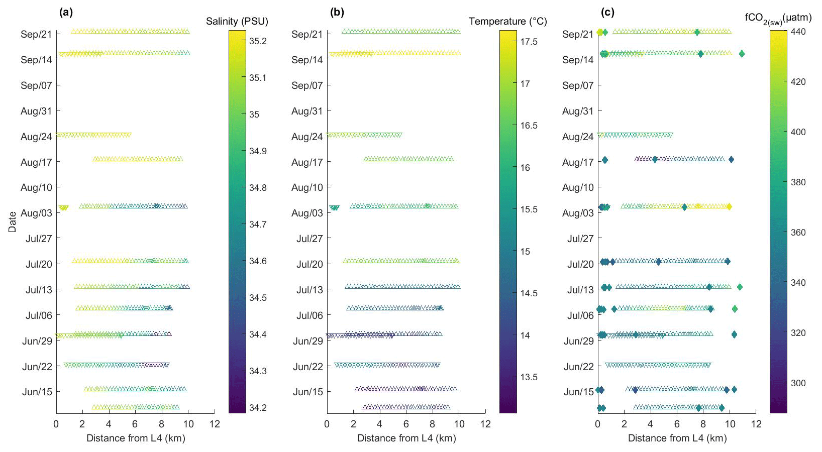
Figure 3 Surface water transects by RV Plymouth Quest between Plymouth Breakwater and station L4 from 10 June to 21 September 2016. Plotted are (a) salinity, (b) temperature and (c) fCO₂ as a function of distance from L4. Outbound transects are shown as downwards triangles, and inbound transects are shown as upwards triangles for salinity, temperature and membrane equilibrator fCO₂ (sampling period = 0.5 min). Showerhead equilibrator fCO₂ observations are denoted by filled diamonds.

3.2 Spatial and temporal variation in salinity, SST and fCO₂

Sea surface salinity at L4 during the June to October study period does show small variation (mean ± SD = 35.15 ± 0.08; Fig. 3a). The L4 salinity range during the study period is within the range of previous years (Smyth et al., 2010b). L4 salinity decreased intermittently, with a maximum reduction of 0.68 on 9 August. The salinity measurements at L4 contrast with the large variability in breakwater salinity during the study period (34.17–35.23). The average salinity difference between the breakwater and L4 is 0.36. The salinity ranges observed at L4 and at the breakwater are similar to model results during a tidal cycle (Uncles et al., 2015).

Coastal SSTs (Fig. 3b) followed the seasonal warming pattern slowly increasing from 13.9 ^∘C on 10 June to 16.7 ^∘C on 21 September. The warming trend was in broad agreement with SST trends observed during previous years (Smyth et al., 2010b). The SST variation along each transect was typically small (< 1 ^∘C) compared to the SST change over the study period (2.8 ^∘C). The smallest temperature difference between L4 and the breakwater (0.025 ^∘C) occurred on 15 September. The largest temperature differences occurred during early summer (1.20, 0.63, 0.59 and 0.65 ^∘C on 10, 15, 22 and 30 June, respectively).

L4 surface fCO₂ increased from 355 to 420 µatm between 10 June and 21 September (Fig. 3c). The average fCO₂ difference between L4 and the breakwater was 20 µatm. Abrupt changes in fCO₂ were observed along the transects, generally close to the breakwater (> 4 km from the L4 station). fCO₂ in waters within 4 km of the breakwater ranged between 338 and 440 µatm during the study period. fCO₂ measurements within 2 km of the PPAO also varied considerably during some of the transects; for example, fCO₂ varied between 337 and 434 µatm during the transect past the PPAO on 7 July. The variability in membrane equilibrator fCO₂ measurements agreed with previous observations in the region (Kitidis et al., 2012).

When transects were ordered by stage along the 12 h tidal cycle, the spatial variability in salinity transects (Fig. S2 in the Supplement) appeared to correspond to the different stages of the tidal cycle. Temperature and fCO₂ transects can be found in the Supplement (Figs. S3 and S4). We divided our transect data according to the stage in the tidal cycle (determined from the Devonport tidal gauge station; 50.368^∘ N, −4.185^∘ W; Fig. 1b). Transects were characterised by the time elapsed since the last period of low water (i.e. LW + X h) using the time at the midpoint of each transect.

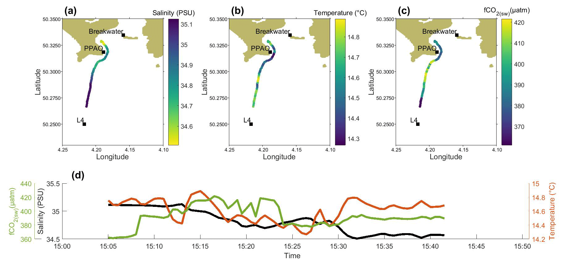
Figure 4 Example of a low water transect (transect midpoint = LW + 0.5 h). Surface measurements of salinity, temperature and fCO₂ represented spatially (a–c) and as a time series (d) from station L4 toward the coast. Data were collected aboard RV Plymouth Quest on 7 July 2016 (filled circles, data every 30 s).

Four categories were used, corresponding to 3 h tidal periods: low water (LW + 0 h), flooding tide (LW + 3 h), high water (LW + 6 h) and ebbing tide (LW + 9 h). Four transects are used below to exemplify the relationship between the different stages of the tidal cycle and the spatial variation in fCO₂ (Figs. 4–7).

3.3 Example transects

The transect on 7 July (low water, LW + 0 h) began at L4 and headed inland (Fig. 4). Salinity was 35.1 close to L4 and declined along the transect. The low salinity was directly north of PPAO (34.7) and in the shallow waters of Cawsand Bay (north of PPAO, 35.5). SST was warmest near L4 and in the relatively shallow Cawsand Bay. The river water was cooler than the L4 seawater, and there was a negative gradient (0.55 ^∘C) into Cawsand Bay. fCO₂ was lowest (∼ 360 µatm) when near to L4 and highest (∼ 430 µatm) immediately south of PPAO. fCO₂ to the north of PPAO in Cawsand Bay was ∼ 390 µatm, which is lower than waters south of PPAO.

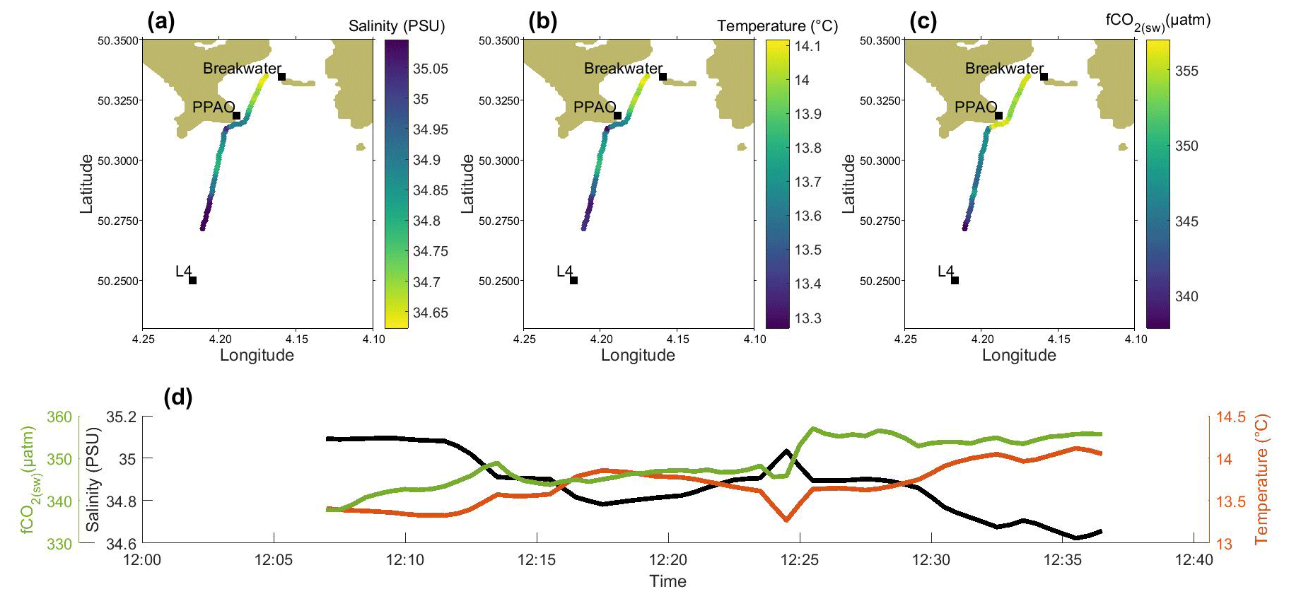
Figure 5 Example of a flooding tide transect (transect midpoint = LW + 3.5 h). Surface measurements of salinity, temperature and fCO₂ represented spatially (a–c) and as a time series (d) from station L4 toward the coast. Data were collected aboard RV Plymouth Quest on 15 June 2016, (filled circles, data every 30 s).

The data collected on 15 June are an example from a flooding tide transect (LW + 3 h, Fig. 5). Salinity was 35.1 in waters close to L4 and decreased toward PPAO and the breakwater (34.7 minimum). The River Tamar plume was warmer than coastal waters in July. SST was highest (∼ 14.1 ^∘C) close to the breakwater, and the coldest water along the transect (13.3 ^∘C) was near to L4. The difference in fCO₂ between L4 and the breakwater was ∼ 18 µatm, with higher fCO₂ (353 µatm) in the warm, low-salinity water close to the breakwater.

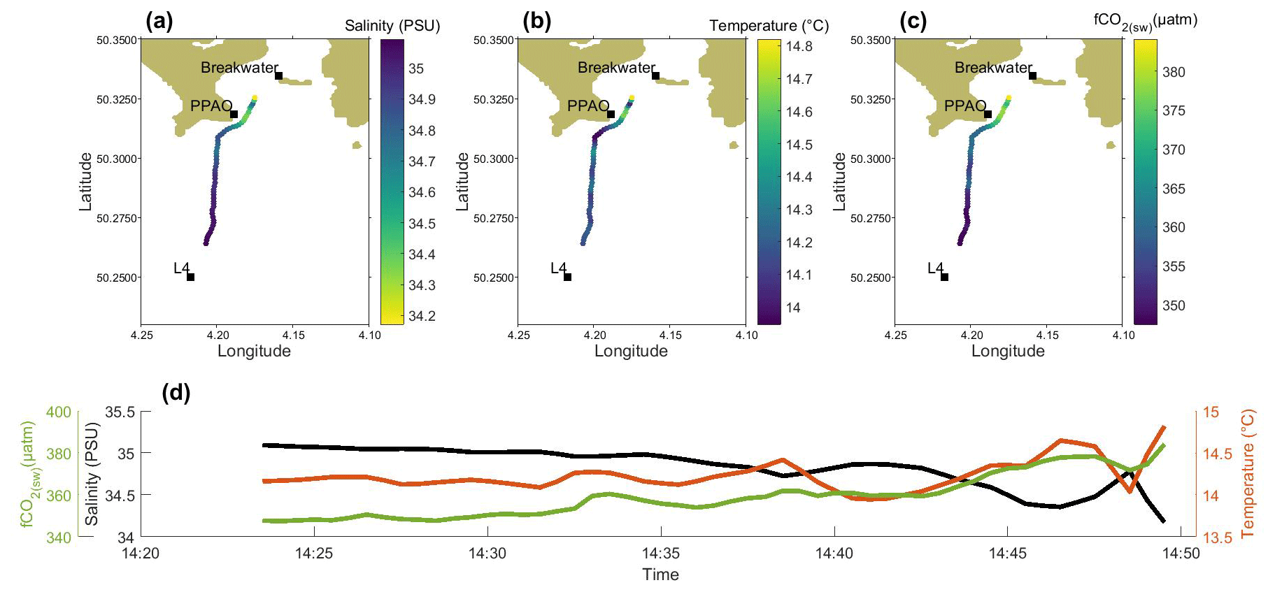
Figure 6 Example of a high water transect (transect midpoint = LW + 6 h). Surface measurements of salinity, temperature and fCO₂ represented spatially (a–c) and as a time series (d) from station L4 toward the coast. Data were collected aboard RV Plymouth Quest on 30 June 2016, (filled circles, data every 30 s).

Data collected on 30 June are an example of a transect at high water (LW + 6 h, Fig. 6). High-salinity (> 35) water was observed much closer to PPAO during the LW + 6 h transect than on transects during low water periods in the tidal cycle (Figs. 4 and 5). Salinity reduces rapidly to 34.1 in between the PPAO and the breakwater. Spatial patterns similar to surface salinity are seen in SST and fCO₂, with the gradients the inverse of the salinity gradient. The low-salinity water close to the breakwater has higher SST and fCO₂ (14.8 ^∘C and 385 µatm) than the observations south of PPAO. The fCO₂ range on this transect was ∼ 38 µatm, and the majority of the change was close to the PPAO. The fCO₂ difference between L4 and the water just south of PPAO was only ∼ 12 µatm. These data suggest that the Tamar plume during LW + 6 h was restricted near to the coast and did not make a big impact upon the waters in between PPAO and L4.

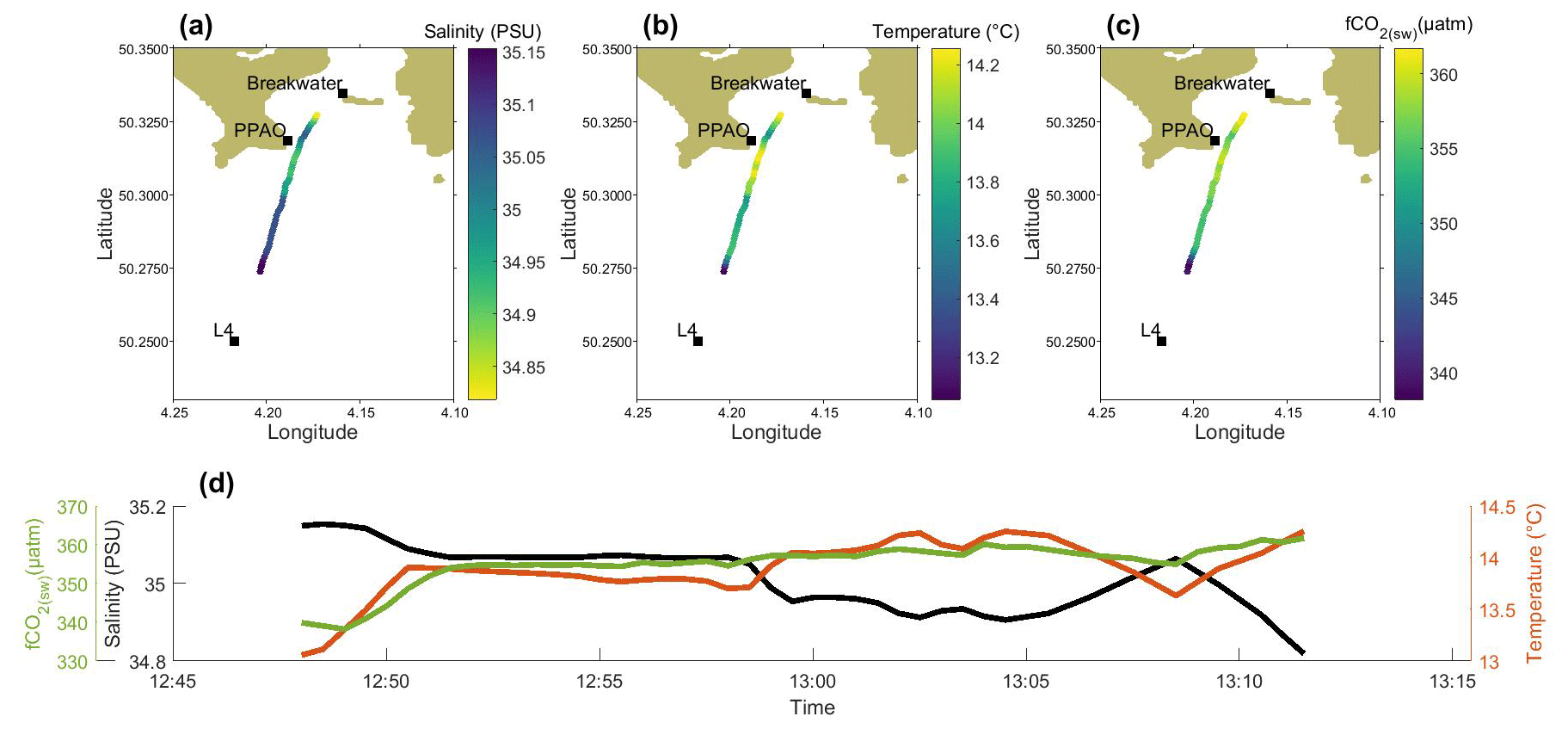
Figure 7 Example of an ebbing tide transect (transect midpoint = LW + 8.75 h). Surface measurements of salinity, temperature and fCO₂ represented spatially (a–c) and as a time series (d) from station L4 toward the coast. Data were collected aboard RV Plymouth Quest on 10 June 2016, (filled circles, data every 30 s).

Data on 10 June show a transect during an ebbing tide (LW + 9 h) (Fig. 7). Salinity near to L4 was 35.15 and declined toward the coast, interrupted by a patch of water due east of PPAO with salinity levels similar to L4. Two patches of low-salinity water (34.8) were encountered along the transect. One low-salinity patch was just south of PPAO and the other patch was close to the breakwater. Spatial variations in SST and fCO₂ coincide with the variations in salinity, with higher SST (∼ 14.2 ^∘C) and fCO₂ (∼ 365 µatm) in the patches of low-salinity water. The fCO₂ difference between L4 surface waters and the fresh, warm waters influenced by the River Tamar plume is ∼ 25 µatm.

In summary, the variations in salinity observed in all transects (i.e. examples above and those in Fig. S2) qualitatively agreed with output from a previous physical model of the Plymouth Sound (Siddorn et al., 2003). The freshwater plume at low water extends out past the PPAO, whereas the plume at high water (LW + 6 h) is restricted to close to the breakwater (Siddorn et al., 2003). The same model on an ebbing tide predicts that two plumes of river water exit via the channels at the east and west ends of the breakwater.

3.4 Relationship between salinity and fCO₂

The changes in salinity and fCO₂ during the example transects suggest that the changes in fCO₂ are driven by conservative mixing of salt water and freshwater endmembers. Robust fCO₂ and salinity relationships have been observed in large river plumes like the Amazon and Mississippi (Lefèvre et al., 2010; Cai et al., 2013). The relationship between salinity and fCO₂ is complicated by the seasonal variability in fCO₂ and the constantly changing position of the tidally controlled freshwater plume. We calculated the difference between in situ data from transects and from measurements at L4 to account for seasonal variations in seawater CO₂:

$$\begin{array}{}\text{(4)}& {\displaystyle }& {\displaystyle }\mathit{\xi }\mathit{\text{f}}{\mathrm{CO}}_{\mathrm{2}}={\text{Transect}}_{\mathit{\text{f}}{\mathrm{CO}}_{\mathrm{2}}}-{\text{L4}}_{\mathit{\text{f}}{\mathrm{CO}}_{\mathrm{2}}},\text{(5)}& {\displaystyle }& {\displaystyle }\mathit{\xi }S={\mathrm{Transect}}_{\mathrm{Salinity}}-\mathrm{L}{\mathrm{4}}_{\mathrm{Salinity}}.\end{array}$$

ξfCO₂ and ξS displayed an apparent relationship throughout different seasons and stages of the tidal cycle (Fig. 8). ξS was a stronger predictor of ξfCO₂ than location along the transect (distance from L4).

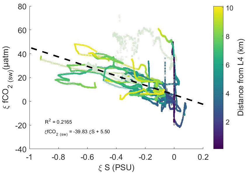
Figure 8 Scatter plot of ξS versus ξfCO₂; difference of data from transects between Plymouth Breakwater and station L4 between 10 June and 21 September 2016. Data are coloured by their distance from station L4; the dashed black line is the best fit for the data. The data for 7 July are shown in light grey.

The fCO₂ and salinity data diverged from the general trend when the RV Plymouth Quest travelled into Cawsand Bay (west of the breakwater) on 7 July (Fig. 8). Uncles and Torres (2013) showed that the seawater residence time increases as you approach the breakwater; following that methodology, the FVCOM model used here also shows this is true for Cawsand Bay. A long residence time and a shallow water column mean that the waters in Cawsand Bay are likely to be closer to equilibrium with the atmosphere due to relatively higher turbulent mixing from bottom stress and surface waves (Upstill-Goddard, 2006). As Cawsand Bay is a microscale environment (< 1 km²), the bay could be a biological hotspot driving the changes in CO₂. Excluding the 7 July transect that went into Cawsand Bay, the linear fit to the ξfCO₂ and ξS data gives ξfCO₂ = −39.83 ξS + 5.50 (R² = 0.2165, N=22 262, p = < 0.001). The fit explained 21.6 % of the variability in the data, with a RMSE of 18.95 µatm.

fCO₂ values calculated from TA and DIC bottle data from the River Tamar on 1 October 2014 show a qualitatively similar relationship between salinity and fCO₂ (Fig. S5 in the Supplement) for stations T3–T9. The trend continues for stations furthest upstream (T1 and T2) but does not follow the same linear relationship. A linear fit between ξS and ξfCO₂ for stations T3–T9 suggests a 42.24 µatm change per unit of salinity. The bottle data indicate that the ξfCO₂ and ξS relationship can be extrapolated to lower salinities and that the relationship begins to break down at ξS < −4. Note that the TA/DIC data and fCO₂ data were collected at different times (years and stages of seasonal cycle) and with different sampling and analytical approaches. The apparent linear relationship between ξfCO₂ and ξS suggested that it can be applied to the wider coastal region. The next section assesses the utility of the high-resolution model (Uncles et al., 2020) to predict coastal fCO₂.

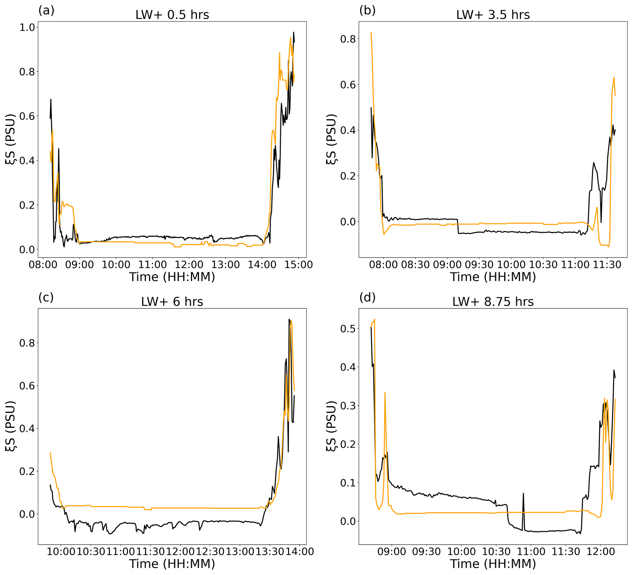
Figure 9 Comparison of ξS from surface observations (underway RV Plymouth Quest, black) and the FVCOM model (orange). Each of the four panels corresponds to the four example transects from four stages of the tidal cycle: (a) 7 July (LW + 0 h), (b) 15 June (LW + 3.5 h), (c) 30 June (LW + 6 h) and (d) 10 June (LW + 8.75 h).

3.5 Using FVCOM to estimate coastal air–sea CO₂ fluxes

Extrapolation of the relationship between ξS and ξfCO₂ across the coastal domain required that FVCOM accurately replicates available surface salinity observations at different stages of the tidal cycle. FVCOM compares very well with the spatial and temporal variability in the four example transects at different stages of the tidal cycle (Fig. 9), even though the hourly resolution of the model means the model output frequency cannot capture subtle changes in frontal positions that are penalised in point-to-point comparisons. Model agreement with the ξS observations (−0.1 > ξS < 4) from all 15 transects was also good (RMSE = 0.213), which indicates that FVCOM can be used as a reliable indication of spatial and temporal salinity changes during the observation period (June–September 2016) (Fig. S6 in the Supplement).

Figure 10 (a) Model surface salinity field on 7 July at the midpoint of the observational transect. Note that the range of the colour bar was restricted to better depict salinity in the lower estuary, and thus salinity in the upper estuaries is beyond the range of the colour bar. (b) Derived ξfCO₂ using the determined ξS and ξfCO₂ relationship.

Modelled spatial variations in coastal surface salinity are shown in Fig. 10a, which focuses on the 7 July transect. Equivalent plots for the other three example transects on 30 June, 15 June and 10 June (Figs. S7 to S9 in the Supplement). The 7 July transect was at low water (LW + 0 h) and when low-salinity water was exiting from either side of the breakwater and wrapping around the Rame Head peninsula (Fig. 10a).

FVCOM output was combined with surface measurements of fCO₂ at L4 (Kitidis et al., 2012) to predict coastal variability in air–sea CO₂ fluxes (Fig. 10b). The model domain for estimated fCO₂ is restricted (i) to cover the region inshore of L4 (> 50.24^∘ N, Fig. 10b), (ii) to avoid regions where gas exchange is largely caused by bottom-driven turbulence (bottom depth > 10 m) and (iii) to avoid over-extrapolating the relationship observed in Fig. 8 (ξS > −4, equivalent to a minimum salinity of approximately 30). The model domain excludes the upper sections of the rivers and the upper estuary and shallow coastal waters such as Cawsand Bay. The model results suggest that the majority of the coastal waters (Plymouth Sound and surroundings) contain fCO₂ levels that are substantially higher (> 100 µatm) than L4 at this stage of the tidal cycle (low water, LW + 0 h).

The standard combined uncertainty for calculated fCO₂ values is consistent with the International Bureau of Weights and Measures (BIPM) guide to the expression of uncertainty in measurement (GUM) methodology (JCGM, 2008). In determining ξS, there is the uncertainty in modelled salinity (Transect_Salinity) given as the RMSE of the model salinity (0.213) and the instrument uncertainty in the salinity at L4 (L4_Salinity for Wetlabs WQM = 0.003; Smyth et al., 2010a), which add in quadrature. The combined model and instrument ξS uncertainty is propagated through the ξfCO₂ and ξS equation to give an uncertainty due to ξS (8.48 µatm). The standard combined uncertainty in fCO₂ includes the uncertainty in the ξfCO₂ and ξS relationship (18.95 µatm), uncertainty due to ξS (8.48 µatm), and the uncertainty in the fCO₂ observations (L4 fCO₂ = 6.9 µatm, from the on station comparison, Fig. 2). These uncertainties add in quadrature to give a standard combined uncertainty of 21.88 µatm.

Figure 11 Modelled impact of a full tidal cycle (a) on tidal height and (b) on air–sea CO₂ flux in the coastal zone (hourly calculations; negative fluxes are into the ocean) on 7 July 2016 with a fixed wind speed of 5.3 m s⁻¹. The total integrated air–sea CO₂ flux within the modelled domain (c–f). Spatial variation in flux at four different stages of the 12 h tidal cycle is shown: LW + 0 h (c), LW + 3 h (d), LW + 6 h (e) and LW + 9 h (f). The red dots in panels (a) and (b) correspond to panels (c)–(f).

The FVCOM model enables simulation of a full tidal cycle so that the impact on air–sea CO₂ flux can be visualised throughout 7 July (Fig. 11; equivalent figures for the examples on 30, 15 and 10 June are in Figs. S10 to S12 in the Supplement). A constant wind speed (equal to the mean during that period) is applied across the model domain (surface area = 132 km²) for simplicity. The flux signal co-varies with tidal height (Fig. 11a and b). The flux integrated across the model domain changes substantially throughout the tidal cycle (∼ 9 % change). If the region is restricted further to include just the area north of PPAO (> 50.32^∘ N), then the magnitude of the flux changes substantially from a weak sink (∼ −65 mol h⁻¹) at low tide to a substantially larger sink (∼ −1100 mol h⁻¹) at high tide.

Figure 12 fCO₂ and pCO₂ values used to calculate the regional CO₂ flux over the domain (128 km², approximately same as in above figures). Measurements of fCO₂ made by RV Plymouth Quest on station at L4 (L4, green dots). pCO_2(atm) measured by RV Plymouth Quest on station at L4 (grey squares). The results of this study; hourly average fCO₂ across the valid model domain used for long-term flux calculations (this study, blue dots). The standard combined uncertainty in the data from this study is indicated by the shaded background in light blue. The monthly Landschützer pCO₂ data (Landschützer coastal product, orange dots) are from the closest valid node (50.125^∘ N, 4.125^∘ W) in the Landschützer et al. (2020) coastal data product. It is noted that the Landschützer node is outside of the model domain (which has a lower boundary of 50.24^∘ N). The vertical dashed lines indicate the dates of the first and last measurement transects.

Three configurations were used to calculate the flux (Fig. 12) to establish whether the tidal plume had a net effect on the regional air–sea fluxes calculated on seasonal timescales between March and November 2016. In the first configuration (L4), L4 measurements were extrapolated across the study area. The second configuration (this study) combined the L4 measurements with the fCO₂ and salinity relationship (Fig. 8) and applied the result to the spatially varying salinity field from the FVCOM model. In the third configuration (Landschützer coastal product), the CO₂ value from closest node (50.125^∘ N, 4.125^∘ W) in the Landschützer coastal product (Landschützer et al., 2020) is extrapolated across the study area. Fluxes were computed for a fixed region of 128 km² (a slight modification of the region in Figs. 10b and 11a–d) encompassing the river plume and the region behind the breakwater. Areas that met the depth and salinity criteria in the region (depth > 10 m, ξS > −4 and > 50.24^∘ N) for > 80 % of the period were included. Whilst fCO₂ is typically measured weekly at L4 by the showerhead system, instrument downtime in 2016 meant that the measurements were less frequent than normal, leading to interpolation between measurements to construct a non-fragmented time series of seasonal fCO₂ in 2016 (an unavoidable limitation of this approach). The average regional fCO₂ (i.e. including using the spatially varying salinity) showed undersaturation in the summer and oversaturation in the spring and autumn. The regional concentration was ∼ 30 µatm greater than the observed concentrations at L4, which is larger than the uncertainty in our estimate of fCO₂ (Fig. 12). The pCO₂ in the Landschützer coastal product was much lower than the observed fCO₂ values at L4 in 2016 (Fig. 12).

L4 pCO₂ saturations (Fig. 12) indicate that fluxes follow the same trend as previous measurements at the site: CO₂ uptake in the region throughout the summer and a short period of outgassing in late September (Kitidis et al., 2012; Marrec et al., 2013). The Landschützer product suggests that the region is a larger sink than indicated by the measurements at L4 and does not indicate that the region is ever a source of CO₂ to the atmosphere. This study calculates fluxes using fCO₂ values predicted from salinity and suggests that the near-coastal region (128 km²) was a weaker sink in summer, increasing the discrepancy with the Landschützer product. This study also suggests weak outgassing of CO₂ near the coast in March, April and October

4 Discussion

Here we show large variations in fCO₂ in the estuarine zone using a high-frequency membrane equilibrator which could not be detected using a showerhead equilibrator. Seawater fCO₂ is assumed to be relatively homogeneous over large spatial scales in the open ocean (Takahashi et al., 2009). Temporal variability in open-ocean waters is also typically slow, with the most rapid variations occurring over hourly or slower timescales (e.g. diurnal Torres et al., 2021). The measuring frequency of a typical showerhead seawater CO₂ system (∼ 8 min) is thus sufficient to determine open-ocean fCO₂ variability. The difference between the underway fCO₂ measurements made by the two systems used in this study (Fig. 2) is caused by the different response times of the showerhead and membrane equilibrators and their ability to resolve the considerable horizontal variability in coastal and shelf waters (Kitidis et al., 2012). The membrane and showerhead systems agreed well when the ship was on station (RMSE = 6.9 µatm), because both systems had sufficient time to equilibrate. When the ship was moving through heterogeneous coastal surface waters, the showerhead system cannot fully equilibrate, and the agreement with the fast-response membrane equilibrator system is worse (RMSE = 27.1 µatm).

Single seawater CO₂ observations are representative of CO₂ integrated across the region that the ship transits through whilst equilibrating. The RV Plymouth Quest typically travels at ∼ 9 knots (4.6 $\mathrm{m}/\mathrm{s}$), which is equivalent to 0.22 km in 48 s (two e-folding times response time of the membrane system) and 1.1 km in 4 min (two e-folding times response time of the showerhead system). However, the showerhead system also switches between seawater CO₂, CO₂ gas standards and atmospheric CO₂; hence, seawater measurements are not continuous. This routine means that seawater fCO₂ measurements are 27 min apart, which equates to a distance of ∼ 7.5 km when the RV Plymouth Quest is moving.

We identified an inverse linear relationship between salinity and fCO₂ and that salinity measurements also agreed well with model salinity output. The FVCOM model output confirms that the river plume extent is highly variable in time and space and that oceanographic features in the region such as the river plume are ∼ 1 km or smaller. The highly dynamic nature of the plume means that a showerhead CO₂ system cannot be expected to resolve the spatial dynamics. A showerhead fCO₂ system design can also be biased toward the end of the equilibration period, which may generate some measurement bias if seawater fCO₂ changes rapidly during the 8 min full equilibration time (e.g. Ribas-Ribas et al., 2014). Complete characterisation of fCO₂ in coastal waters within 10 km of land and with highly variable fCO₂ requires a system with a fast-response equilibrator or slower steaming.

Mixing of estuarine and continental shelf water masses partially determines the fCO₂ levels observed in this nearshore study region. Shelf waters exhibit a seasonal surface fCO₂ trend associated with (a) cooling-enhanced solubility in late winter, (b) net phytoplankton uptake in spring/summer, (c) partial re-equilibration with the atmosphere and (d) mixing with CO₂-rich bottom waters in autumn (Kitidis et al., 2019). The River Tamar is the other mixing endmember and is typically oversaturated with fCO₂ with respect to the atmosphere (Frankignoulle et al., 1998). The results presented in this paper also suggest that riverine fCO₂ may have a strong influence on the spatial and temporal patterns in coastal waters off Plymouth. It is important to note that the relationship between salinity and fCO₂ determined in this paper only explains 21.6 % of the variability and was derived with summer data only (due to sampling constraints). Further work is needed to confirm if the relationship holds during the remaining period of the year (i.e. October through to May).

The fCO₂ variability that is not explained by our relationship could be driven by other factors. Close to the coast such as in Cawsand Bay, these include gas exchange in shallow waters, changes in CO₂ concentration in the river, excess river runoff during storms, CO₂ production in sediments, upwelling of water with different CO₂ concentration and biological activity stimulated by nutrients in the Tamar plume. Biological processes in coastal ecosystems can strongly influence seawater CO₂ levels (Cai et al., 2020), which may explain some of the large CO₂ changes observed around L4 that are not linked to salinity changes. fCO₂ changes due to photosynthesis are typically a few micro-atmospheres per day (Kitidis et al., 2019), so large differences will likely have built up over time. Water masses with fCO₂ levels different to L4 may well be caused by factors such as biological activity and then the water advected toward L4 by currents.

The confluence of estuarine and continental shelf waters near the PPAO/breakwater and the local circulation of surface waters are dominated by the semi-diurnal tidal cycle (Uncles et al., 2015). The rising tide after low water pushes shelf water toward the breakwater, whereas a falling tide after high water encourages riverine-influenced water to extend south. The tidal influence upon coastal fCO₂ is evident in the 15 transects during this study, with changes of 20–40 µatm relative to L4 (Fig. 8). Time series data presented by Borges and Frankignoulle (1999) indicate a similar magnitude (20–25 µatm) tidal signature in coastal Belgian and Dutch waters.

The salinity field from the FVCOM model is used to estimate the surface fCO₂ features over a complete tidal cycle and shows that the flux can change by a non-trivial amount (∼ 9 %) over a short period of time (Fig. 11). These data also show that using a hydrodynamic model can extend the spatial and temporal coverage of CO₂ uptake and outgassing estimates in the coastal region surrounding Plymouth made with weekly L4 measurements (Fig. 12). If similar relationships can be developed for other estuarine zones, then operational dynamic models may also be able to add information to flux estimates for these zones. The spatial resolution of the model at the surface means that it is possible that near-surface features such as freshwater lenses are overlooked by this analysis. Higher-resolution modelling of the surface ocean would make future coastal products more applicable to air–sea flux studies.

5 Conclusions

Here we show for the first time dynamic and large variations in the coastal zone using a fast-response membrane equilibrator system. These gradients between estuarine waters and shelf waters were not resolved by a co-located showerhead CO₂ system. The gradients in salinity and fCO₂ fields show strong tidal influence. Changes in fCO₂ after accounting for the seasonal trend are linked with salinity variations, with the highest regions of fCO₂ coinciding with the lowest salinity regions and vice versa. The inverse linear relationship between salinity and fCO₂ variations (Fig. 8) suggests that mixing of estuarine and shelf water endmembers is a control on the surface water distribution of fCO₂. Measured salinity agrees well with FVCOM model surface salinity fields at different stages of the tidal cycle. FVCOM output is used to estimate the temporal and spatial variations of fCO₂ in coastal waters. The model output demonstrates that neglecting the river plume leads to an overestimation of the magnitude of the CO₂ sink in the summer. The region may also be misidentified as a sink for atmospheric CO₂ in the spring and autumn when it could be a weak source, as suggested by Torres et al. (2020). Measurements from L4 are not representative of the estuarine zone, and caution should be used when scaling them over this region.

The surface flux from estuaries and coastal waters has proven difficult to assess comprehensively (Borges et al., 2006). The high-resolution fCO₂ data presented in this study show that tidal and estuarine-influenced coastal waters can quickly transition from a strong source to a strong sink depending on the state of the tide (Fig. 11). Inland and coastal waters are a large uncertainty in global fluxes (Chen et al., 2013). The high-resolution observations presented in this paper show that the head of the river/estuarine plume for this region is linked to the tidal state. This is critical for the accurate calculation of air–water flux from the region. Further studies are required to evaluate the wider applicability of this method to similar coastal regions. Distinctly different estuarine/coastal zones such as lagoons, river deltas and fjords will have their own distinct fCO₂ signatures and patterns driven in part by surface water circulation and mixing. High-resolution models that can resolve tides and surface salinity in estuarine/coastal waters with high confidence are a useful tool in ongoing and future efforts to constrain coastal air–sea CO₂ fluxes.