Climate pathways behind phytoplankton-induced atmospheric warming

We investigate the ways in which marine biologically mediated heating increases the surface atmospheric temperature. While the effects of phytoplankton light absorption on the ocean have gained attention over the past years, the impact of this biogeophysical mechanism on the atmosphere is still unclear. Phytoplankton light absorption warms the surface of the ocean, which in turn affects the air–sea heat and CO₂ exchanges. However, the contribution of air–sea heat versus CO₂ fluxes in the phytoplankton-induced atmospheric warming has not been yet determined. Different so-called climate pathways are involved. We distinguish heat exchange, CO₂ exchange, dissolved CO₂, solubility of CO₂ and sea-ice-covered area. To shed more light on this subject, we employ the EcoGEnIE Earth system model that includes a new light penetration scheme and isolate the effects of individual fluxes. Our results indicate that phytoplankton-induced changes in air–sea CO₂ exchange warm the atmosphere by 0.71 ^∘C due to higher greenhouse gas concentrations. The phytoplankton-induced changes in air–sea heat exchange cool the atmosphere by 0.02 ^∘C due to a larger amount of outgoing longwave radiation. Overall, the enhanced air–sea CO₂ exchange due to phytoplankton light absorption is the main driver in the biologically induced atmospheric heating.

1 Introduction

Previous studies have shown that marine biota can modify the light penetration in the ocean with consequences on the atmospheric temperature and on the climate system (Shell et al., 2003; Wetzel et al., 2006; Gnanadesikan and Anderson, 2009). Using an Earth system model (ESM) of intermediate complexity, we identify and compare the climate pathways behind the changes in atmospheric temperature due to phytoplankton light absorption.

Marine biota and phytoplankton play a major role in the absorption of light and therefore in the vertical distribution of heat in the upper layers of the ocean (Kowalczuk et al., 2019). Indeed, observational evidence supports the hypothesis that chlorophyll increases the upper ocean heat uptake. For instance, satellite observations show that phytoplankton blooms can cause an increase in sea surface temperature (SST) of 1.5 ^∘C (Kahru et al., 1993). Furthermore, previous remote sensing data indicate an increase in local SST of 4.5 ^∘C on a 4 d timescale due to the presence of phytoplankton blooms (Capone et al., 1998). Recent high-resolution in situ observations in the Indo-West Pacific Ocean highlight large anomalies of temperature of 0.95 ^∘C in the uppermost skin layer of the ocean when large phytoplankton blooms appear (Wurl et al., 2018). However, all these observations are either on a short timescale or in a geographically limited area. To study the larger-scale impact of phytoplankton light absorption and its relative magnitude, Earth system models are employed.

Models of differing complexity are used to study the effect of phytoplankton light absorption. For instance, using ocean-only (Anderson et al., 2007) or general circulation models, several studies focusing on the tropical Pacific Ocean (Murtugudde et al., 2002; Lengaigne et al., 2007; Löptien et al., 2009) or on the Arctic Ocean (Lengaigne et al., 2009) report an increase in SST between 0.5–2 ^∘C due to phytoplankton light absorption. A warming of the ocean surface induced by marine biota has consequences on the overall climate system. For instance, Patara et al. (2012) find that an increase in SST due to phytoplankton light absorption increases the atmospheric humidity content thereby increasing the greenhouse effect and the atmospheric temperature locally by up to 0.5 ^∘C. Furthermore, phytoplankton can amplify locally the seasonal temperature of the lowest atmospheric layer by 1 ^∘C, changing the Walker and Hadley circulation (Shell et al., 2003).

It is therefore known that phytoplankton light absorption plays a non-negligible role in the atmospheric temperature, but which climate pathway is the most important behind this warming is still unclear. Phytoplankton light absorption affects the surface atmospheric temperature via two climate pathways. First, various modeling studies suggest that biologically induced surface water heating can increase the air–sea heat exchange (Capone et al., 1998; Oschlies, 2004; Wetzel et al., 2006) with consequences on the formation of tropical storms and monsoons in the Arabian Sea (Sathyendranath et al., 1991). Second, the solubility of gases and thus also the air–sea CO₂ exchange is affected by phytoplankton light absorption. For instance, Manizza et al. (2008) study the impact of this biogeophysical mechanism on the air–sea flux of CO₂ and find that phytoplankton light absorption has a small outgassing effect on a global scale with high regional fluctuations.

However, none of these studies have analyzed, disentangled and compared the changes in both air–sea heat and CO₂ exchange due to phytoplankton light absorption. To shed light on the biologically induced atmospheric warming, we use a recent Earth system model called EcoGEnIE (Ward et al., 2018). In an earlier study, we implemented phytoplankton light absorption in this model (Asselot et al., 2021). We consider two different biologically induced changes: changes in air–sea heat and changes in air–sea CO₂ exchange (Fig. 1). The air–sea CO₂ exchange can be influenced by the dissolved oceanic CO₂ in three different ways: (1) through changes in the biogeochemical pumps as a result of phytoplankton light absorption – for instance, Manizza et al. (2008) have shown that changes in oceanic circulation due to phytoplankton light absorption enhance the vertical supply of nutrients, increasing the relative abundance of calcifiers, and as a consequence, the primary production and the export production of organic matter increase; (2) through a decrease in CO₂ solubility due to higher SST, increasing the atmospheric CO₂ concentrations and the greenhouse gas effect; and (3) through a decrease in sea-ice formation, because sea ice acts as an ocean cap that blocks gas exchanges. To achieve the disentangling of the specific climate pathways, we turn them on and off by prescribing values in our ESM in order to isolate their impact on the climate system.

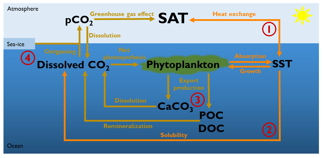
Figure 1 Representation of the four different biologically induced pathways that affect the atmospheric temperature. (1) Marine biota via phytoplankton light absorption increases the SST, changing therefore the air–sea heat exchange and the atmospheric temperature. (2) Changes in SST also alter the solubility of CO₂ and its dissolved concentration. In turn, changes in dissolved CO₂ concentrations alter the air–sea CO₂ exchange and thus the greenhouse gas effect. (3) Phytoplankton light absorption modifies the marine biogeochemical cycles and particularly the export production of carbon. These changes in export production of carbon modify the dissolved CO₂ concentration and the greenhouse gas effect. (4) A warmer surface of the ocean can decrease the sea-ice extent. A reduction of sea-ice cover increases the air–sea CO₂ exchange area, changing the greenhouse gas concentrations. SAT: surface atmospheric temperature. SST: sea surface temperature. CaCO₃: calcium carbonate. POC: particulate organic carbon. DOC: dissolved organic carbon.

2 Model description

Our motivation is to study the interactions between the marine ecosystem, the biogeochemistry, the biogeophysics and the climate system. These interactions are computationally expensive in high-resolution models; therefore we used an Earth system model of intermediate complexity (Claussen et al., 2002). The Earth system model employed is the carbon-centric Grid-Enabled Integrated Earth system model (cGEnIE) (Lenton et al., 2007) composed of several modules describing the dynamics of the Earth system (Fig. 2). This model has been previously calibrated and compared to observations (Edwards and Marsh, 2005; Lenton et al., 2006; Ridgwell et al., 2007; Marsh et al., 2011). Moreover, this model is widely used to study past climate and changes in the carbon cycle over geological times (Ödalen et al., 2018; Greene et al., 2019; Adloff et al., 2020), past mass extinctions (Alvarez et al., 2019) and biogeochemistry processes (Meyer et al., 2016). Additionally, cGEnIE has been employed to assess the sensitivity of atmospheric CO₂ to biogeochemical pumps, ocean circulation and climate feedbacks in the Southern Ocean (Cameron et al., 2005). A new ecosystem component (ECOGEM) is associated with cGEnIE to form the recent EcoGEnIE model (Ward et al., 2018). EcoGEnIE is used to determine the link between the marine plankton ecosystem and various past climate scenarios (Wilson et al., 2018) with a focus on phosphorus inventory (Reinhard et al., 2020). For our study, the model combines different components including ocean hydrodynamics, atmosphere, sea ice, ocean biogeochemistry and marine ecosystem. We do not consider a terrestrial component meaning that the land surface is essentially passive. We use the same configuration as described in detail by Asselot et al. (2021), and the following description only refers to our specific model setup.

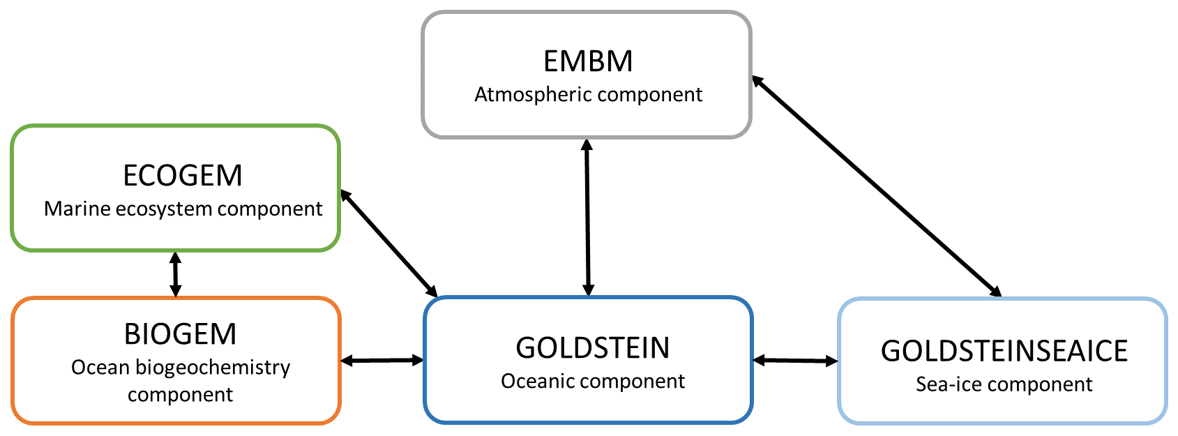
Figure 2 Representation of the components of the EcoGEnIE model. The black arrows indicate the link between the different climatic components.

2.1 Modules

2.1.1 The physical components

The physics of the model contains a frictional-geostrophic ocean circulation (GOLDSTEIN), coupled to a 2D energy–moisture balance model of the atmosphere (EMBM) and a thermodynamic sea-ice model (GOLDSTEINSEAICE) (Edwards and Marsh, 2005; Marsh et al., 2011). Heat and moisture are exchanged between the three components and act as a coupling strategy.

The oceanic component calculates the horizontal and vertical redistribution of heat, salinity and biogeochemical elements via advection, convection and mixing. The ocean module is configured on a 36×36 horizontal grid. The horizontal grid is uniform in longitude and uniform in sine latitude, giving ∼3.2^∘ latitudinal increments at the Equator increasing to 19.2^∘ in the highest latitude. This horizontal grid has been used for previous biogeochemical simulations (Cameron et al., 2005; Colbourn, 2011). We consider 32 vertical oceanic layers increasing logarithmically from 29.38 m for the surface layer to 456.56 m for the deepest layer. This vertical resolution is already used to study the relative importance of biogeophysical and biogeochemical mechanisms on the climate system (Asselot et al., 2021). The atmospheric component is based closely on the UVic Earth system model (Weaver et al., 2001). The prognostic variables are atmospheric temperature and specific humidity. Precipitation removes instantaneously all moisture corresponding to an excess above a relative humidity threshold. The wind stress is prescribed and identical between all simulations; the temperature cannot affect the wind stress. The sea-ice component solves the equation for part of the ocean covered by sea ice. The prognostic variables are ice thickness and ice areal fraction. The transport of sea ice includes sources and sinks of these variables. The growth or decay of sea ice depends on the net heat flux into the ice. The dynamics in this module consist of advection by currents and diffusion. Sea ice does not limit the penetration of photosynthetically available radiation in the ocean.

2.1.2 Ocean biogeochemistry component

The biogeochemical module (BIOGEM) represents the transformation and spatial redistribution of biogeochemical tracers (Ridgwell et al., 2007). The state variables are inorganic and organic matter. The biological uptake is represented by an implicit biological community: nutrients are directly converted into organic matter via an uptake rate. The biological uptake is limited by light, temperature and nutrient availability. Organic matter is partitioned into dissolved and particulate phases (DOM and POM). For this study, BIOGEM does not consider a temperature dependency on iron solubility and iron bioavailability. Our model setup includes iron (Fe) and phosphate (PO₄) as limiting nutrients. Similar to Asselot et al. (2021), we do not consider nitrate here. Moreover, the surface production is redistributed in the water column as a depth-dependent flux. To achieve this, the surface export is divided between refractory organic matter remineralized close to the seafloor and labile organic matter mostly remineralized in the upper water column (Ridgwell et al., 2007). Furthermore, because we do not consider a sediment component, all organic matter reaching the sea floor is instantaneously remineralized. Calcium carbonate (CaCO₃) is represented in the model, and its dissolution below the surface follows the same profile as the remineralization of POM. Additionally, CaCO₃ production is parameterized as a fixed ratio to POC production and so is not independent in our model setup. Recent studies have implemented and calibrated a temperature-dependent remineralization in the model (Crichton et al., 2021; Armstrong McKay et al., 2021), but this parameterization is not included in our model setup. Furthermore, BIOGEM calculates the air–sea CO₂ and O₂ exchange. The value of atmospheric CO₂ predicted by BIOGEM is used as input for the radiative scheme of the atmospheric component, thus providing climate feedback.

2.1.3 Ecosystem component

The marine ecosystem component (ECOGEM) represents the marine plankton community and associated interactions within the ecosystem (Ward et al., 2018). The biological uptake in ECOGEM replaces the BIOGEM uptake calculation and is limited by light, temperature and nutrient availability. Plankton biomass and organic matter are subject to processes such as resource competition and grazing before being passed to DOM and POM. Several ecophysiological parameters are size-dependent such as maximum nutrient uptake rate, cell carbon quotas, grazing, and partitioning between DOM and POM. Additionally, the nutrient uptake, photosynthesis and predation are temperature-dependent. The ecosystem is divided into different plankton functional types (PFTs) with specific traits. Each PFT is sub-divided into size classes with specific size-dependent traits. Here, we consider only two PFTs: phytoplankton and zooplankton (Appendix A1). Phytoplankton is characterized by nutrient uptake and photosynthesis, whereas zooplankton is characterized by predation traits. Zooplankton grazing depends on the concentration of prey biomass, with predominant grazing on prey that are 10 times smaller than themselves. Each population is associated with biomass state variables for carbon, phosphate, iron and chlorophyll. The production of dead organic matter is a function of mortality and messy feeding, with partitioning between non-sinking dissolved and sinking particulate organic matter. Finally, plankton mortality is reduced at very low biomass such that plankton cannot become extinct.

2.2 Light absorption in the ocean

In the previous model version (Ward et al., 2018), light was only absorbed by phytoplankton. In the model version of Asselot et al. (2021), a new light scheme is implemented where the absorbed light by phytoplankton is converted into heat and is able to affect the oceanic temperature. Furthermore, light absorption takes place throughout the water column and is not restricted to the first oceanic layer anymore. The light absorption scheme is a coupling between Eqs. (1) and (2). For simplicity, in our model configuration, the incoming shortwave radiation does not vary seasonally. We look at long-term changes in the climate system; therefore the absence of a seasonal cycle does not affect the overall qualitative and main findings. The presence of organic and inorganic particles as well as dissolved molecules restrains the light penetration in the ocean (Ward et al., 2018). The vertical light attenuation scheme is given by Eq. (1):

$$\begin{array}{}\text{(1)}& I\left(z\right)=I_{\mathrm{0}}\cdot \exp (-k_{\mathrm{w}}\cdot z-k_{\mathrm{Chl}}\cdot \underset{\mathrm{0}}{\overset{z}{\int }}\mathrm{Chl}(z)\cdot \mathrm{d}z),\end{array}$$

where I(z) is the irradiation of the full solar spectrum at depth z, I₀ is the irradiation at the surface of the ocean, k_w is light absorption by clear water and inorganic particles (0.04 m⁻¹), k_Chl is the light absorption by chlorophyll (0.03 m⁻¹(mg Chl)⁻¹), and Chl(z) is the chlorophyll concentration at depth z. The values for k_w and k_Chl are taken from Ward et al. (2018). The parameter I₀ is negative in the model, because it is a downward flux from the sun to the surface of the ocean. We allow primary production and light to penetrate until the sixth layer of the model (221.84 m deep), which is the lower limit of the euphotic zone (Tett, 1990). In our model setup, maximum absorption occurs in the upper oceanic layer and minimum absorption occurs in the sixth layer.

Phytoplankton changes the optical properties of the ocean (Sonntag and Hense, 2011) through phytoplankton light absorption. Therefore it can cause a radiative heating and change the oceanic temperature. We implemented phytoplankton light absorption into the model following Hense (2007) and Patara et al. (2012). The scheme is given by Eq. (2):

$$\begin{array}{}\text{(2)}& {\displaystyle \frac{\partial T}{\partial t}}={\displaystyle \frac{\mathrm{1}}{\mathit{\rho }\cdot c_p}}{\displaystyle \frac{\partial I}{\partial z}}.\end{array}$$

$\partial T/\partial t$ denotes the temperature changes, c_p is the specific heat capacity of water, ρ is the ocean density and I is the solar radiation incident at depth z. Part of the light absorbed is used by phytoplankton for photosynthesis and part leads to heating of the water.

2.3 Air–sea heat exchange

We detail here the total heat flux from the ocean and sea ice going into the atmosphere. The vertically integrated atmospheric heat equation (Eq. 3) is given by Weaver et al. (2001) and Marsh et al. (2011):

$$\begin{array}{}\text{(3)}& Q_{\mathrm{ta}}=Q_{\mathrm{SW}}\cdot C_{\mathrm{A}}+Q_{\mathrm{LH}}+Q_{\mathrm{LW}}+Q_{\mathrm{SH}}-Q_{\mathrm{PLW}}.\end{array}$$

Q_ta corresponds to the total heat flux into the atmosphere, Q_SW is the net shortwave radiation corresponding to the solar irradiance received from the sun and reflected by the planet's albedo, C_A is a heat absorption coefficient (0.3 over the ocean; Marsh et al., 2011), Q_LH is the latent heat flux corresponding to phase change of a thermodynamic system, Q_SH is the sensible heat flux corresponding to temperature change of a thermodynamic system, Q_LW is the net (upward minus downward) re-emitted longwave radiation corresponding to infrared energy coming from the planet and Q_PLW is the outgoing planetary longwave radiation.

The atmosphere loses heat through net longwave radiation, dominated by the outgoing longwave radiation; thus the total longwave heat flux (Q_LW+Q_PLW) is negative in the model. Furthermore, evaporative cooling of the ocean leads to a latent heat release in the atmosphere upon condensation and precipitation. Evaporated water vapor may be transported away from an oceanic source, to condense and precipitate elsewhere.

2.4 Air–sea CO₂ exchange

The atmospheric temperature depends on the atmospheric CO₂ concentration which is affected by the transfer of CO₂ between the ocean and the atmosphere. The flux of CO₂ across the atmosphere–ocean interface (Eq. 4) is given by Ridgwell et al. (2007):

$$\begin{array}{}\text{(4)}& F_{{\mathrm{CO}}_{\mathrm{2}}}=k\cdot \mathit{\rho }\cdot (C_w-\mathit{\alpha }\cdot C_{\mathrm{a}})\cdot (\mathrm{1}-A).\end{array}$$

$F_{{\mathrm{CO}}_{\mathrm{2}}}$ is the air–sea CO₂ flux, k corresponds to the gas transfer velocity, ρ is the ocean density, C_w is the concentration of dissolved gas in the surface ocean, α is the solubility coefficient calculated from Wanninkhof (1992) and depends on the sea surface temperature and salinity, C_a is the concentration of gas in the atmosphere, and A is the fraction of the ocean covered by sea ice. Phytoplankton light absorption warms the surface of the ocean and thus reduces CO₂ solubility and sea-ice fraction. The flux of CO₂ is therefore affected via the parameters C_w, α and A. To study the flux precisely we either prescribe these parameters in the air–sea CO₂ exchange calculation or let them evolve freely (see below).

3 Model setup and simulations

During this study, we are primarily interested in the relative differences between our selected simulations. We focus on the relative impact of phytoplankton light absorption on different climate pathways rather than on the changes in the climate state. We try to simulate realistic mean climate systems but the absolute values of the climate quantities are less relevant due to the limitations of such a model of intermediate complexity.

For a realistic nutrient distribution in the ocean, we performed a BIOGEM spin-up for 10 000 years. During the spin-up the atmospheric CO₂ concentration is fixed to 278 ppm. The simulations restart for 1000 years after the spin-up with ECOGEM, meaning that all simulations consider marine biota. Due to the single-layer atmospheric component, the non-seasonality and the non-representation of the land dynamics, running the model for 1000 years is sufficient to achieve a steady state. The results represent the annual mean of the last year of the simulations, when the model is in a steady state. The present-day continental configuration, model setup, grid resolution and ecosystem community are identical as in Asselot et al. (2021). Our model setup has a reasonable match to observations, and further details can be found in Asselot et al. (2021). For simplification, only one phytoplankton and one zooplankton species are included in the model setup (Appendix A1 and B1). Repeating our main simulations with multiple size classes leads to small differences compared to the simulations with one size class (Appendix B1). Unlike our previous study, prescribing SST is necessary for some simulations here. Due to technical issues, we cannot prescribe the seasonal cycle of SST but only the annually averaged SST. As a consequence, the seasonality is removed from our model setup. The absence of the seasonal cycle is not an issue for this study because we look at the importance of each climate pathway rather than focusing on the quantitative changes of the climate system.

The carbon cycle is closed in our simulations, meaning that there is no input of carbon through volcanic or anthropogenic activities. Only the size of the carbon reservoirs can vary. If not stated otherwise, the concentration of atmospheric CO₂ evolves freely in the simulations. All simulations are forced with the same constant flux of dissolved iron into the ocean surface (Mahowald et al., 2006). To ensure that the model is suitable for our study, we conducted two sensitivity analyses. First, we analyzed the sensitivity of the climate variables by conducting two simulations with different atmospheric CO₂ concentrations (Appendix C1). Second, we ensure that the heat and CO₂ interaction is negligible (Appendix D1). To study the effect of phytoplankton light absorption on the atmospheric temperature we perform seven different simulations, all including the ECOGEM component (Fig. 3):

• Bio is the reference run and is the only simulation that does not include phytoplankton light absorption (k_Chl=0 in Eq. 1). In this simulation, all the climate pathways evolve freely.

• BioLA is the same as the reference run but phytoplankton light absorption is implemented. In this simulation, all the climate pathways evolve freely.

• HEAT is the same as the second one except that we prescribe the atmospheric CO₂ concentration only for the atmospheric temperature calculation. For a comparison with the reference run, the prescribed atmospheric CO₂ concentration from Bio is used (169 ppm). The effect of CO₂ on atmospheric temperature is fixed but the air–sea heat fluxes evolve freely. This simulation analyses the effect of phytoplankton-induced changes of air–sea heat fluxes on the atmospheric temperature.

• CARB is the simulation with an uncoupled ocean–atmosphere setup. The atmospheric component is forced with the heat fluxes from Bio and the atmospheric CO₂ concentration is prescribed with the value of BioLA. This simulation determines the effect of phytoplankton-induced changes of atmospheric CO₂ concentration on the atmospheric temperature. Please note that CARB is well suited for studying the atmospheric properties but not to examine ocean dynamics.

• HCorg is the simulation where we only allow the biogeochemical pumps (soft-tissue pump and carbonate pump) to affect the dissolved CO₂. The solubility of CO₂ (α in Eq. 4) and sea-ice extent (A in Eq. 4) parameters are prescribed using the respective values from Bio. The CO₂ solubility is fixed by prescribing the SST only for this calculation. In HCorg air–sea heat exchange and the biogeochemical pumps parameter (C_w in Eq. 4) evolve freely.

• HCorgSI is the simulation where the biogeochemical pumps and sea-ice extent affect dissolved CO₂. The CO₂ solubility (α in Eq. 4) is prescribed using the value of Bio. In HCorgSI the air–sea heat exchange, the biogeochemical pumps (C_w in Eq. 4) and sea-ice extent (A in Eq. 4) parameters evolve freely.

• HCorgSol is the simulation where the biogeochemical pumps and the solubility pump affect dissolved oceanic CO₂. The sea-ice extent parameter (A in Eq. 4) is prescribed using the value of Bio. In HCorgSol the air–sea heat exchange, the biogeochemical pumps (C_w in Eq. 4) and the CO₂ solubility (α in Eq. 4) parameters evolve freely.

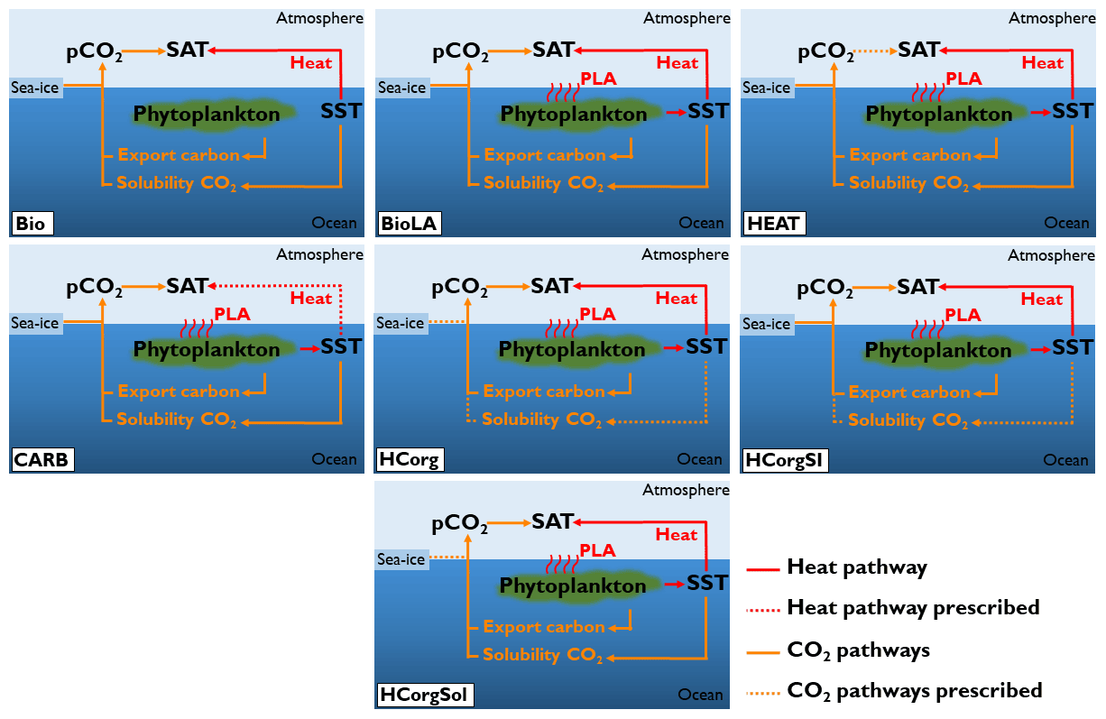
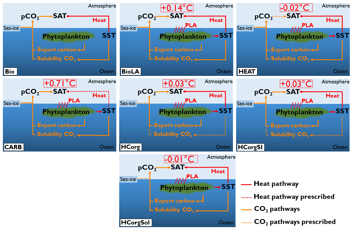
Figure 3 Sketch representing the climate pathways involved in the seven simulations (PLA: phytoplankton light absorption). Note that this figure is a simplification of Fig. 1; only the relevant pathways are represented. The name of the simulations are on the bottom left of each panel. The dashed arrows indicate the climate pathways prescribed. All the prescribed pathways are from the reference simulation Bio except the pathway between atmospheric CO₂ and SAT in CARB, which is prescribed from the simulation BioLA.

4 Global response of the climate system

In this section we present the results of the simulations on a global scale. We do not consider local patterns because we removed any seasonal cycle in our model setup. Moreover, the horizontal grid resolution is low and marine biota cannot move between grid cells; thus even if seasonality was included, key regional patterns will not be resolved. First, we focus on the chlorophyll biomass and sea surface temperature, because phytoplankton light absorption has a direct effect on these climate variables (Oschlies, 2004; Lengaigne et al., 2007; Paulsen et al., 2018). Second, these changes in oceanic properties affect the carbon cycle (Manizza et al., 2008; Asselot et al., 2021); therefore we study the changes in atmospheric CO₂ concentration. Third, phytoplankton light absorption alters the atmospheric properties (Patara et al., 2012); thus we analyze the changes in radiative heat fluxes, humidity and evaporation. Finally, the response of the surface atmospheric temperature is analyzed.

4.1 Chlorophyll biomass and sea surface temperature

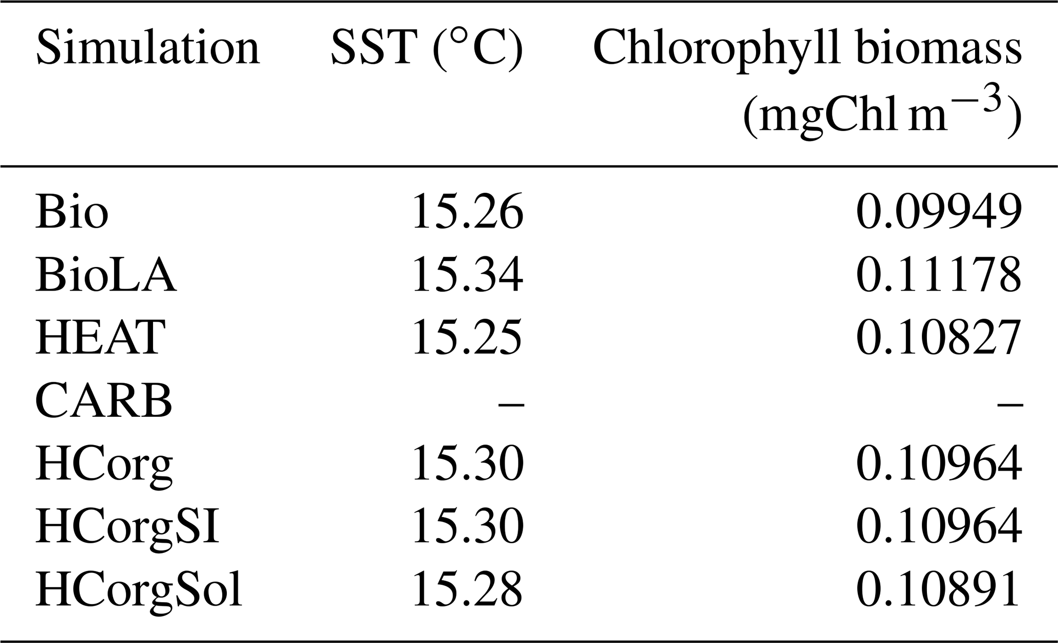
Our results indicate differences of SST and chlorophyll biomass, depending on the climate pathways included in our model setup (Table 1). Due to the uncoupled ocean–atmosphere setup in CARB, ocean dynamics are not presented in this section. The reference run Bio has the lowest chlorophyll biomass and a low SST while the simulation BioLA has the highest chlorophyll biomass and SST. The increase in chlorophyll biomass is due to two different mechanisms: first, phytoplankton light absorption leads to a higher surface production, enhancing the remineralization at the surface of the ocean as shown by Asselot et al. (2021). Second, phytoplankton light absorption enhances the upward vertical velocity in the upwelling regions. As a result of these two mechanisms, the surface nutrient concentrations increase, explaining the higher chlorophyll biomass. The increase in surface chlorophyll biomass due to phytoplankton light absorption between BioLA and Bio is 0.012 mgChl m⁻³, in line with a previous estimate of 0.014 mgChl m⁻³ (Asselot et al., 2021). The higher chlorophyll biomass is, however, limited by the increase in zooplankton biomass applying a top-down control. Via the effect of phytoplankton light absorption, a higher surface chlorophyll biomass leads to an increase in SST. The global difference of SST between BioLA and Bio is 0.08 ^∘C. This value is lower than previous model estimates that show a global SST increase of 0.45–1 ^∘C due to phytoplankton light absorption (Murtugudde et al., 2002; Löptien et al., 2009; Asselot et al., 2021). This underestimation of the biologically induced SST increase is due to the non-seasonal radiative forcing of the model, decreasing the global heat budget (Appendix E1).

In HEAT, the chlorophyll biomass is higher while the SST is lower compared to Bio (Table 1). This is rather counter-intuitive and is due to changes in oceanic circulation between these two simulations. For instance, the maximum Atlantic meridional overturning circulation (AMOC) is 8.6 Sv in HEAT while it is 7.6 Sv in Bio. In HEAT, the SST is lower and the sea-ice cover is slightly higher (Appendix F1) compared to Bio, leading to more deep water formation in polar latitudes. As a result, the AMOC is enhanced in HEAT. The stronger oceanic circulation in HEAT leads to an enhanced nutrient redistribution, thus increasing the surface nutrient concentrations. For instance, the surface PO₄ concentration is ∼0.21 µmol kg⁻¹ in HEAT while it is ∼0.19 µmol kg⁻¹ in Bio. The higher surface PO₄ concentration in HEAT explains the higher chlorophyll biomass in this simulation compared to Bio. The enhanced oceanic circulation in HEAT compared to Bio also leads to a stronger redistribution of heat along the water column, explaining the surface cooling and the warming of the deep ocean in HEAT. Our results indicate that the bottom water temperature in HEAT is 3.57 ^∘C while it is 3.09 ^∘C in Bio.

The surface chlorophyll biomass in the simulations HCorg, HCorgSI and HCorgSol are higher than the surface chlorophyll biomass in Bio due to the higher surface PO₄ concentrations. In Bio the surface PO₄ concentration is 0.18 µmol kg⁻¹ while in the simulations HCorg, HCorgSI and HCorgSol the surface PO₄ concentrations are >0.21 µmol kg⁻¹. The higher surface PO₄ concentrations are due to enhanced remineralization at the ocean surface and enhanced upward vertical velocities in the upwelling regions. Due to the effect of phytoplankton light absorption, the higher surface chlorophyll biomasses in HCorg, HCorgSI and HCorgSol lead to higher SSTs compared to Bio. Only the sea-ice extent differs between the simulations HCorg and HCorgSI, but their chlorophyll biomass and SSTs are identical. This result evidences a lack of sea-ice influence on these climate variables and thus on the heat fluxes. In addition, the chlorophyll biomass and SST are higher in HCorg compared to HCorgSol, indicating that the solubility factor has a negative effect on these climate variables. Between these two simulations, the only difference is the CO₂-solubility factor that can evolve freely in HCorgSol. In the simulation HCorg, the SST for the calculation of the CO₂ solubility is prescribed using the value of Bio, which is the lowest value. Considering the physical and chemical properties of the ocean, a low SST increases the solubility of CO₂ (Wanninkhof, 1992). Therefore, the CO₂ solubility is reduced in HCorgSol compared to HCorg, due to the higher SST in HCorgSol. For instance, our results indicate that on a global scale, the surface oceanic CO₂ concentration is 27.200 µmol kg⁻¹ in HCorgSol while it is 27.213 µmol kg⁻¹ in HCorg. Via the nutrient ratios, these changes in carbon cycle between the simulations affect the phosphate and iron cycles (Ward et al., 2018). As a consequence, the surface PO₄ concentration is ∼0.216 µmol kg⁻¹ in HCorg and ∼0.214 µmol kg⁻¹ in HCorgSol. The higher surface PO₄ concentration leads to a larger surface chlorophyll biomass and higher SST in HCorg compared to HCorgSol.

Table 1 Sea surface temperature (^∘C) and surface chlorophyll biomass (mgChl m⁻³). There is no value for the simulation CARB because we run the model with an uncoupled ocean–atmosphere setup.

4.2 Atmospheric properties

The oceanic properties differ between the simulations; thus we expect differences in the atmospheric properties. We compare the atmospheric CO₂ concentration, the heat fluxes, the evaporation, the specific humidity and finally the surface atmospheric temperature between the simulations.

4.2.1 Atmospheric CO₂ concentration

The atmospheric CO₂ concentrations for the simulations is low compared to the pre-industrial level (Fig. 4). This is due to our new model setup that allows primary production until the sixth oceanic layer, meaning that more carbon is stored in the deep ocean, reducing the atmospheric CO₂ concentration (see Asselot et al., 2021). In all the simulations considering phytoplankton light absorption, the atmospheric CO₂ concentration is higher than in the reference run. In a previous study, we evidence that the higher atmospheric CO₂ concentration is mainly due to a decrease in CO₂ solubility via the higher SST while the enhanced remineralization of organic matter and the dissolution of CaCO₃ affect the atmospheric CO₂ concentration slightly (Asselot et al., 2021). The atmospheric CO₂ concentration is the lowest in Bio while it is the highest in BioLA, with a difference of 9 ppm. This value is lower than a previous estimate that indicates an increase in atmospheric CO₂ concentration of 18 ppm (Asselot et al., 2021). This lower estimate is due to the non-seasonal cycle forcing, neglecting the seasonal variations of air–sea CO₂ exchanges.

In HEAT, the atmospheric CO₂ concentration is prescribed only for the atmospheric temperature calculation. Therefore the atmospheric CO₂ concentration can vary due to changes in dissolved oceanic CO₂, sea-ice extent and CO₂ solubility, affecting the other climate variables. The atmospheric CO₂ concentration in HEAT is slightly higher than in Bio. This is due to the larger chlorophyll biomass in HEAT than in Bio (Table 1), indicating a higher production and thus more remineralization in the ocean. During the remineralization process, CO₂ is produced; thus the higher remineralization in HEAT increases the dissolved CO₂ concentration. On a global scale, our results indicate that the surface dissolved oceanic CO₂ is about 6.354 mol kg⁻¹ in HEAT, while it is 6.302 mol kg⁻¹ in Bio. The larger dissolved oceanic CO₂ concentration in HEAT increases the air–sea CO₂ flux and in turn the atmospheric CO₂ concentration (see Eq. 4).

The atmospheric CO₂ concentration in CARB is similar to the one in BioLA, because we prescribed the value against the one in BioLA.

The simulations HCorg, HCorgSI and HCorgSol have a higher atmospheric CO₂ concentration than in Bio. This is again not surprising because these simulations consider phytoplankton light absorption, which increases the atmospheric CO₂ concentration as shown by Asselot et al. (2021). The atmospheric CO₂ concentration between HCorg and HCorgSI is similar even if their sea-ice extent and sea-ice thickness differs (Appendix F1). The changes in sea ice do not have an effect on the atmospheric CO₂ concentration. The slightly higher atmospheric CO₂ concentration in HCorgSol compared to HCorg is due to changes in CO₂ solubility: as described above, the CO₂ solubility is lower in HCorgSol compared to HCorg. As a consequence, the air–sea CO₂ flux is higher in HCorgSol compared to HCorg, leading to a slightly higher atmospheric CO₂ concentration in HCorgSol.

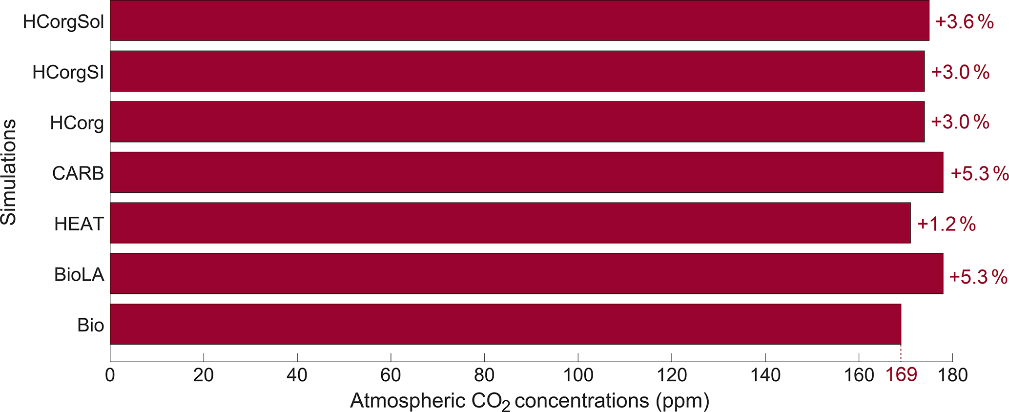
Figure 4 Atmospheric CO₂ concentrations (ppm) for the different simulations. The percentages represent the relative changes compared to the reference simulation Bio.

4.2.2 Heat fluxes

The air–sea heat flux is divided into the net shortwave radiation, the net re-emitted longwave radiation, the sensible heat flux and the latent heat flux (Fig. 5). The air–sea heat fluxes represent the total heat fluxes from the ocean and sea ice, going into the atmosphere. The simulations HCorg and HCorgSI have exactly the same heat fluxes. The only difference between these two simulations is the different sea-ice extent for the calculation of the air–sea CO₂ flux. This change in air–sea CO₂ flux does not alter the air–sea heat flux, explaining the identical radiative heat fluxes between HCorg and HCorgSI. Furthermore, the simulations BioLA and HCorgSol have the same heat fluxes, and the only difference is also the sea-ice extent. As detailed previously, the changes in sea-ice extent do not affect the heat fluxes, explaining the identical radiative fluxes between BioLA and HCorgSol. Finally, the heat fluxes between CARB and Bio are identical because we prescribed the heat fluxes in CARB with the values of Bio.

The net shortwave heat flux is divided into two fluxes: the incoming shortwave radiation from the sun entering the atmosphere and the outgoing reflected shortwave radiation leaving the atmosphere. Figure 5a shows that the net shortwave heat flux is identical for all the simulations and is positive. The positive values indicate that net shortwave heat flux is dominated by the flux entering the system, the incoming radiation. The incoming shortwave radiation from the sun is always identical between simulations. Therefore identical net shortwave heat flux implies that the outgoing reflected shortwave radiation is also the same between simulations due to the treatment of shortwave radiation in the model (Weaver et al., 2001).

The net longwave heat flux is negative for all simulations, indicating that this flux is dominated by the upward longwave radiation leaving the atmosphere (Fig. 5b). A more negative value of net longwave heat flux indicates a greater loss of heat to outer space. The simulations Bio and CARB have the least negative net longwave heat flux, while HEAT has the highest negative heat flux, indicating that HEAT loses more heat than the other simulations. The higher heat loss in HEAT is due to the lowest SST and a reduced amount of greenhouse gases, specifically a low specific humidity (Fig. 6) and atmospheric CO₂ concentration (Fig. 4). The lower amount of greenhouse gases in the atmosphere permits a higher loss of heat outside the atmosphere. All the simulations considering phytoplankton light absorption, except CARB where the heat fluxes are prescribed, have a higher negative net longwave heat flux compared to Bio. This result is predictable because this biogeophysical mechanism is an additional heat source for the surface of the ocean, where air–sea heat exchanges occur.

The sensible heat flux depends on the atmospheric and oceanic temperature (Fanning and Weaver, 1996; Weaver et al., 2001). The sensible heat flux increases when the atmospheric temperature decreases and when the oceanic temperature increases. For the simulation HEAT, the sensible heat flux is the highest (Fig. 5c), because the atmospheric temperature is the lowest (Fig. 7). In contrast, the sensible heat flux is the lowest for the simulation BioLA, because the gradient of temperature between the ocean and the atmosphere is low. The sensible heat fluxes in HCorg and HCorgSI are close to the sensible heat flux of Bio because their air–sea temperature gradients are almost similar.

The global mean latent heat flux (Fig. 5d) depends mainly on the global mean precipitation (Weaver et al., 2001). The simulation Bio has the smaller latent heat flux due to the lowest precipitation in this simulation (Appendix G1). The latent heat fluxes in BioLA, HCorg, HCorgSI and HCorgSol are almost similar due to their almost similar precipitation values. The precipitation in HEAT is higher than in Bio, explaining the higher latent heat flux in HEAT.

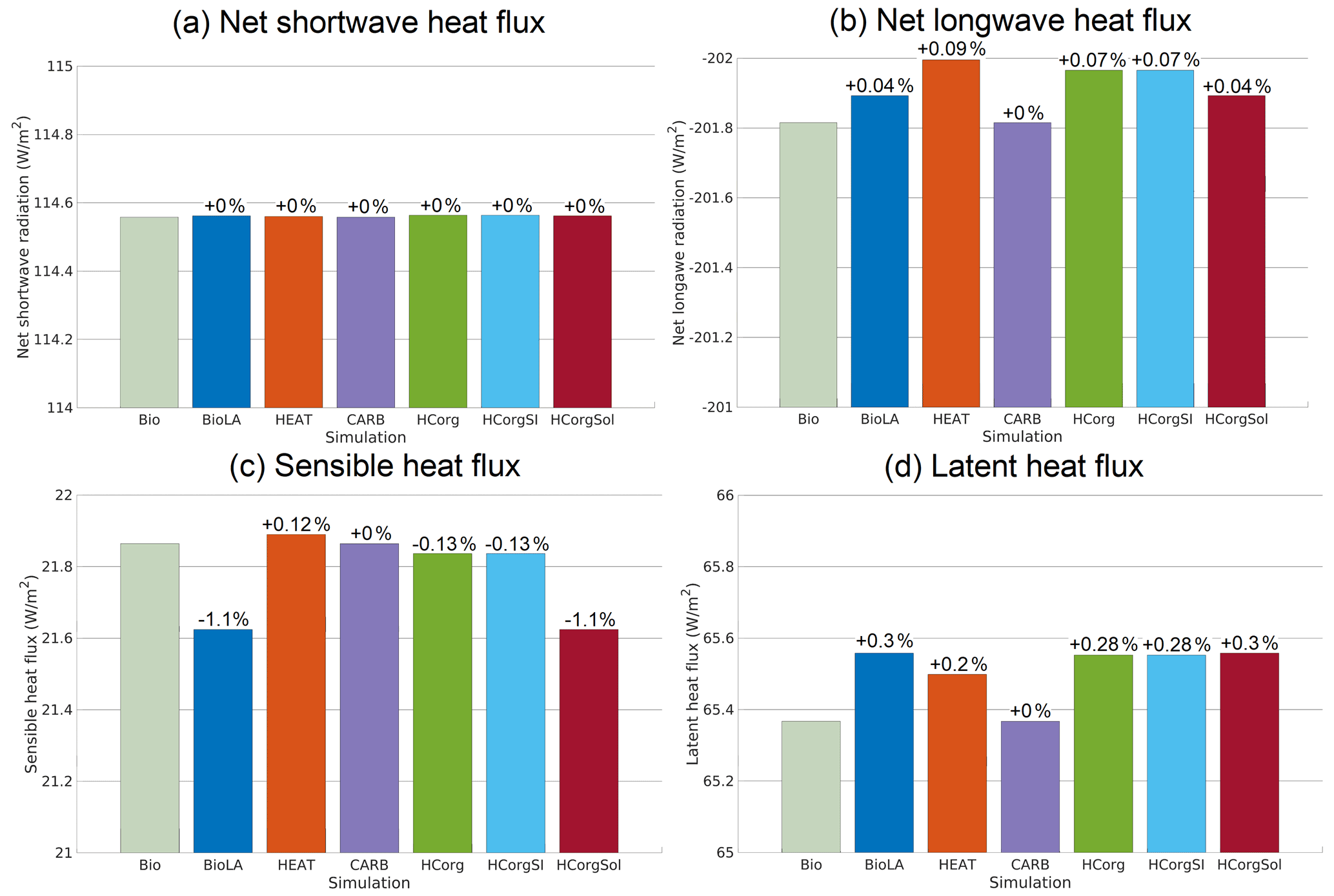
Figure 5 Global average of the different air–sea heat fluxes (W m⁻²) for the seven simulations. (a) Net shortwave radiation at the top of the atmosphere. (b) Net re-emitted longwave radiation. The net longwave radiation is negative, because it is dominated by the outgoing longwave radiation. (c) Sensible heat flux. (d) Latent heat flux. The color coding between the panels remains the same. The percentages represent the relative changes compared to Bio.

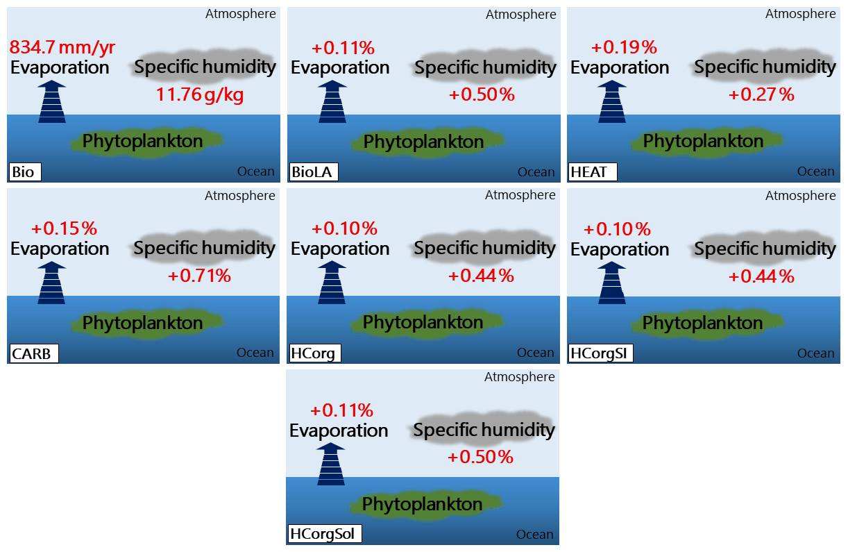
Figure 6 Evaporation (mm yr⁻¹) and specific humidity (g kg⁻¹) for the seven simulations. The percentages represent the relative changes compared to Bio. The name of the simulations are on the bottom left of each panel.

4.2.3 Specific humidity and evaporation

The specific humidity and the evaporation in BioLA and HCorgSol are similar, and the same is true between the simulations HCorg and HCorgSI (Fig. 6). The specific humidity and evaporation are the lowest in Bio due to the lowest latent heat flux in this simulation. Including phytoplankton light absorption increases the latent heat flux and therefore increases the specific humidity and evaporation, which is consistent with Oschlies (2004) and Lengaigne et al. (2009). On a global scale, in BioLA the evaporation increases by 0.11 %, thus enhancing the specific humidity by 0.5 %. This latter value is lower than previous estimates where phytoplankton light absorption raises the specific humidity by 2 %–6 % (Patara et al., 2012). The different values between our estimates and Patara et al. (2012) come from the non-seasonal cycle in our model setup, changing the heat budget and therefore underestimating the specific humidity. Moreover, the specific humidity in HEAT is lower than in BioLA due to the lower latent heat flux in the simulation HEAT. The evaporation depends on several processes, and one of the most important is the humidity in the atmosphere, with lower humidity leading to higher evaporation (Weaver et al., 2001). As a consequence, the evaporation is higher in HEAT than in BioLA. Furthermore, the specific humidity and the evaporation increase when the atmospheric temperature rises (Weaver et al., 2001). The specific humidity and evaporation are higher in CARB compared to BioLA because the surface atmospheric temperature is higher in CARB (Fig. 7). The specific humidity and evaporation in HCorg and HCorgSI are slightly lower than in BioLA because the latent heat flux in HCorg and HCorgSI is slightly lower. Once the CO₂ solubility factor is considered (simulation HCorgSol), the values of the specific humidity and evaporation are similar to the values in BioLA. This is not surprising because the heat fluxes between HCorgSol and BioLA are identical.

Figure 7 Sketch representing the surface atmospheric temperature (SAT) changes between the simulations and the reference run. On top is located the value of SAT change compared to Bio. The rest of the sketch is similar to Fig. 3.

4.2.4 Surface atmospheric temperature

The difference in atmospheric properties between simulations lead to changes of the surface atmospheric temperature (Fig. 7). First of all, Bio has a low SAT because it does not include the additional heat source coming from the phytoplankton light absorption mechanism. The SAT in Bio is 9.31 ^∘C, while the SAT in BioLA is 9.45 ^∘C, which makes a global difference of 0.14 ^∘C. This estimate is lower than previous estimates of 0.2–0.45 ^∘C (Patara et al., 2012; Asselot et al., 2021) due to the non-seasonal cycle in our model.

The lower SAT in HEAT compared to Bio is due to several reasons. Even if HEAT considers phytoplankton light absorption, we show that the SST in HEAT is lower than in Bio. For the SAT computation, the atmospheric CO₂ concentrations are identical between Bio and HEAT. Additionally, the specific humidity only increases by 0.27 % in HEAT compared to Bio. Therefore the greenhouse gas effect between these two simulations is rather similar. However, the global net longwave heat flux decreases by ∼0.2 W m⁻² in HEAT due to the lower SST, leading to a cooling of the atmosphere. The combination of these different reasons explains the slightly lower SAT in HEAT compared to Bio.

For the simulation CARB, the concentration of greenhouse gases (atmospheric CO₂ and specific humidity) is higher than in Bio, while the air–sea heat fluxes are identical. As a consequence, more heat is trapped in the atmosphere, and the SAT increases by 0.71 ^∘C compared to the reference run.

The sea-ice extent is different between HCorg and HCorgSI (Appendix F1), but the response of SAT is identical, indicating that with our model setup, the changes in sea-ice extent do not affect the SAT. The specific humidity and the atmospheric CO₂ concentration are slightly higher in HCorg and HCorgSI, leading to a small increase in SAT compared to Bio.

In HCorgSol the atmospheric CO₂ concentration and the specific humidity are higher than in Bio. However, the sensible heat flux and the net longwave heat flux are lower in HCorgSol. Even if the greenhouse gas concentrations are higher, the reduced air–sea heat fluxes lead to a slight decrease in SAT in the simulation HCorgSol compared to Bio.

5 Limitations

Our study is designed to understand the climate pathways behind phytoplankton-induced atmospheric warming, but our model setup has limitations. Most notably, we do not consider a seasonal cycle in our study. Enabling seasonality would lead to larger seasonal increase in temperature, but it would also lead to larger seasonal decrease in CO₂ solubility. Therefore, we suppose that the heat pathway would not overrule the CO₂ pathway. Due to our new model setup with primary production allowed until the sixth layer of the model, the atmospheric CO₂ concentration of the simulations is lower than the pre-industrial level. Our quantitative estimates would be affected if the atmospheric CO₂ concentration of the reference run were higher, but we assume that the qualitative estimates would be very similar and the conclusions will not change. If the atmospheric CO₂ baseline is higher, the heat budget would also increase. As a consequence, the ocean would be warmer and the CO₂ solubility would decrease, increasing the importance of the CO₂ pathway in the phytoplankton-induced atmospheric warming.

This study investigates the impact of short-lived seasonal organisms; thus having an annual mean approach underestimates the effect of phytoplankton light absorption on the climate system. The absence of a nitrogen cycle could have additional effects that are not included in our study. Phytoplankton light absorption warming low-oxygen regions causes an additional oxygen consumption, leading to hypoxia. As a consequence, we suggest that the denitrification would increase nitrogen fixation inducing a local increase in biomass. This increase in biomass would increase any pathway sensitivity of atmospheric CO₂. Moreover, several studies considering a dynamic land component and focusing on phytoplankton light absorption report an increase in heat budget due to this biogeophysical mechanism (Anderson et al., 2007; Lengaigne et al., 2009). If a land model were to be included, we speculate that we would still find oceanic and atmospheric heating. However, the magnitude of changes might be smaller due to the uptake of CO₂ by vegetation, decreasing the atmospheric CO₂ concentration. Furthermore, the model does not include a temperature-dependency of iron bioavailability. According to previous experiments, a warming of the ocean decreases the bioavailability of iron (Liu and Millero, 2002). Phytoplankton light absorption increasing oceanic temperature might thus reduce the iron bioavailability. As a consequence, the limitation of phytoplankton growth by iron would increase, limiting the increase in chlorophyll biomass due to phytoplankton light absorption. Our study only considers two PFTs, and bringing in more PFTs would be an interesting complement to our findings. For instance, observations and modeling studies indicate that positively buoyant phytoplankton groups, such as cyanobacteria, are important to study phytoplankton light absorption (Sonntag and Hense, 2011; Paulsen et al., 2018; Wurl et al., 2018). Implementing these microorganisms to assess our research question could be a beneficial follow-up of our study.

6 Conclusions

For the first time, using the EcoGEnIE model (Ward et al., 2018), we compare the role of the air–sea heat and CO₂ fluxes and quantify their influence on the biologically induced atmospheric warming. We show that without any seasonality and with all the climate pathways included, the surface atmospheric temperature increases by 0.14 ^∘C due to phytoplankton light absorption. As suggested by previous studies (Capone et al., 1998; Oschlies, 2004; Wetzel et al., 2006), phytoplankton light absorption changes the air–sea heat flux. Our results indicate that when only this air–sea interaction is considered, the atmosphere cools by 0.02 ^∘C compared to a simulation without the biogeophysical mechanism. Moreover, when only the air–sea CO₂ exchange is considered, the atmospheric temperature increases by 0.71 ^∘C. Clearly, our results indicate that the air–sea CO₂ exchange has a more important effect than the air–sea heat flux on the phytoplankton-induced warming of the atmosphere. With our model setup, the sea-ice extent and thickness slightly vary between simulations; therefore sea-ice processes hardly affect the air–sea CO₂ flux and thus the climate system. Moreover, including the solubility pathway changes the heat fluxes, specifically reducing the sensible heat flux and the net longwave heat flux compared to the reference simulation. As a consequence, this climate pathway has a negative effect on the atmospheric temperature. To conclude, phytoplankton light absorption influences the climate pathways at the ocean–atmosphere interface, particularly the air–sea CO₂ exchange that is important for the phytoplankton-induced atmospheric warming. For future climate studies, this work evidences that to capture the overall effect of climate-relevant mechanisms such as phytoplankton light absorption, the atmospheric CO₂ concentrations should evolve freely.

For future work, more studies with higher-complexity models are necessary to make quantitative assessments rather than qualitative assessments as in our study. Similar simulations must be conducted with a seasonal variation of the shortwave radiation to better understand the role of phytoplankton in the climate system. Moreover, a model with a dynamic atmosphere such as PLASIM-GEnIE (Holden et al., 2016) could be a good aspiration to complete our study. Indeed, previous studies evidence either an increased wind speed in subpolar regions (Patara et al., 2012) or enhanced atmospheric dynamics (Wetzel et al., 2006; Gnanadesikan and Anderson, 2009) due to phytoplankton light absorption. The increased wind speed with a dynamic atmospheric component could thus increase the air–sea CO₂ flux, reinforcing the importance of the CO₂ pathway in our study. Finally, implementing the new temperature-dependent remineralization scheme (Crichton et al., 2021; Armstrong McKay et al., 2021) would affect the biological pump and would be an extension to our findings.

Appendix A: Plankton functional types

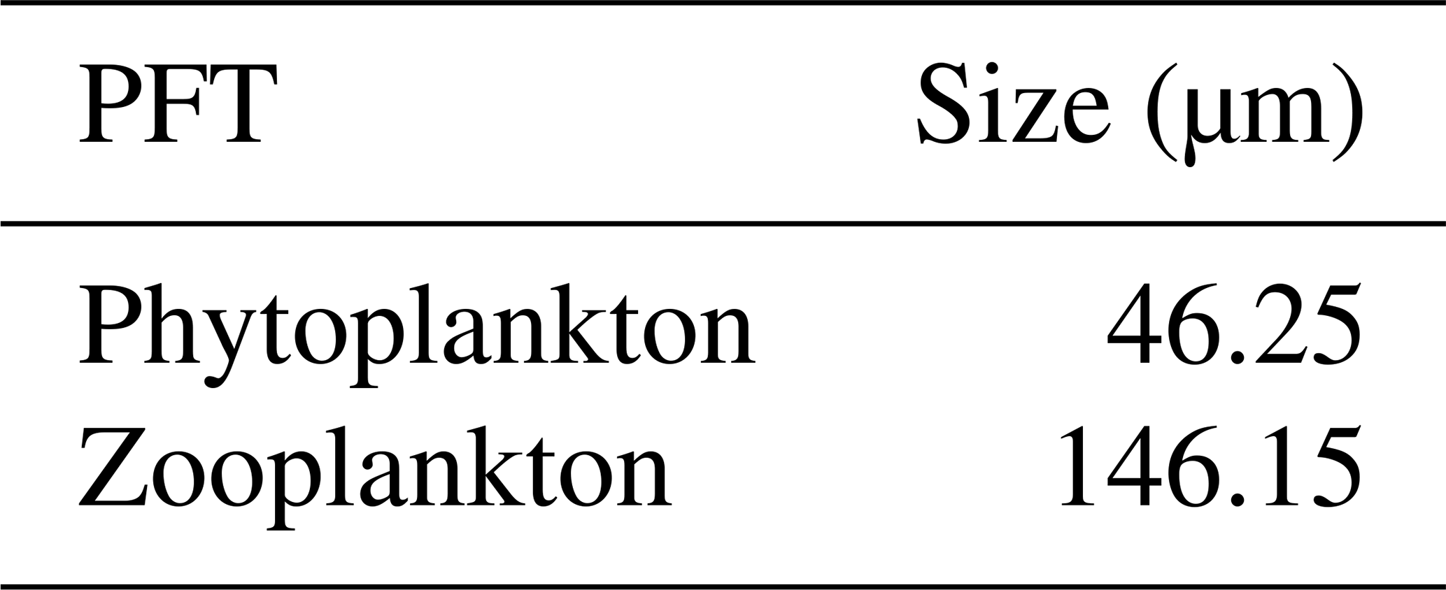
We base our ecosystem community on the community described by Ward et al. (2018). However, instead of using two plankton functional types (PFTs) with eight different size classes, we only use two PFTs with one size class (Appendix A1). We show that introducing more size classes has a smaller effect on the climate system than phytoplankton light absorption (Asselot et al., 2021). Therefore we reduced the ecosystem complexity to increase the computational time of the model.

Table A1 Size of the different plankton functional types (µm) used during the simulations.

Appendix B: Multiple size classes

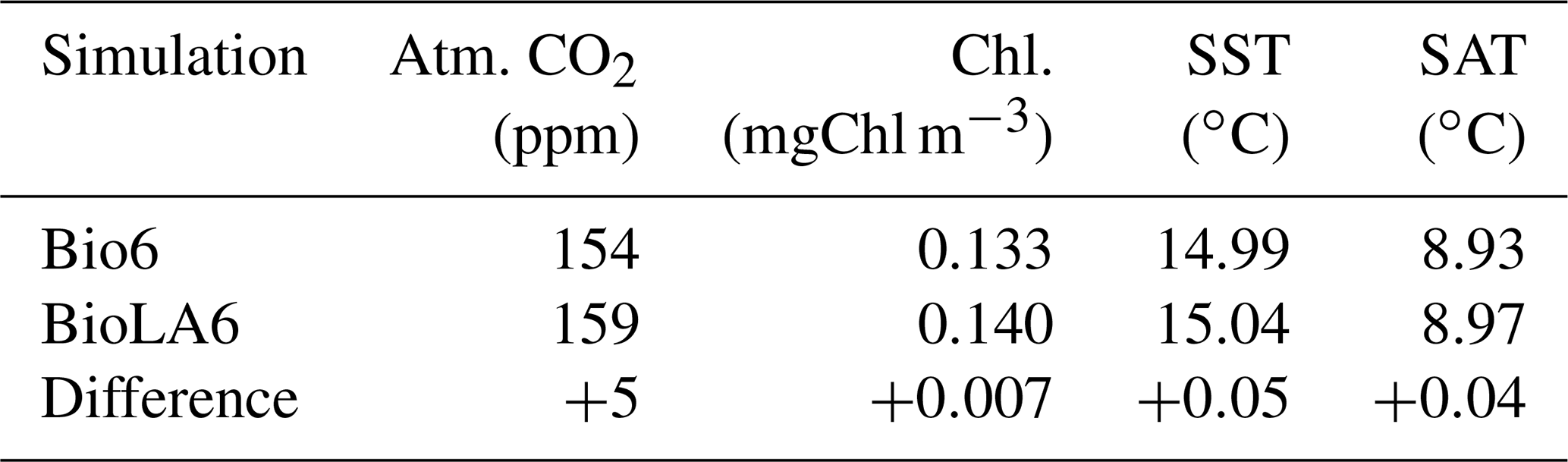
We conduct two additional simulations with a higher ecosystem complexity. These simulations have six phytoplankton and six zooplankton size classes as in Asselot et al. (2021). The simulation BioLA6 considers phytoplankton light absorption, while the simulation Bio6 does not consider it. The results show that the effect of phytoplankton light absorption is reduced with a higher ecosystem complexity compared to the effect of phytoplankton light absorption with a simple ecosystem community. This is due to the higher amount of carbon stored in the living biomass with an increasing number of species, thus reducing the effect of phytoplankton light absorption on the atmospheric CO₂ concentration and on the climate system.

Table B1 Values of the most important climate quantities for the simulations with six phyto- and six zooplankton size classes. The third row represents the differences between the simulation with minus the simulation without phytoplankton light absorption.

Appendix C: Sensitivity of the climate variables

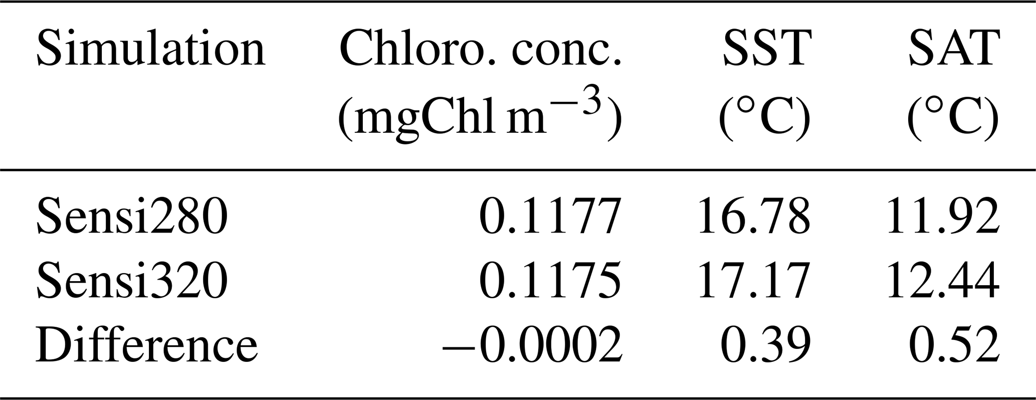
To analyze the sensitivity of the climate variables, we perform two sensitivity analyses (Appendix C1). Both simulations have the same model setup and restart from the spin-up described previously, but their atmospheric CO₂ concentrations differ. The first simulation (Sensi280) has an atmospheric CO₂ concentration of 280 ppm, while the second one (Sensi320) has an atmospheric CO₂ concentration of 320 ppm. Furthermore, the simulations Sensi280 and Sensi320 consider phytoplankton light absorption. An increase of 40 ppm in atmospheric CO₂ concentration slightly reduces the chlorophyll concentration, but these changes are negligible, indicating that surface chlorophyll biomass is more sensitive to phytoplankton light absorption than an increase of 40 ppm in pCO₂. The oceanic and atmospheric heat budgets are affected by the changes in atmospheric CO₂ concentration. Increasing the greenhouse gas concentrations increases in turn the SAT and therefore the SST due to the exchange of heat between the ocean and the atmosphere.

Table C1 Chlorophyll concentration (mgChl m⁻³), sea surface temperature and atmospheric surface temperature (^∘C) for the sensitivity analysis of the climate. The difference represents the value of Sensi320 minus the value of Sensi280.

Appendix D: Air–sea fluxes interactions

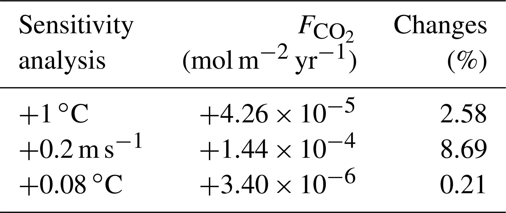
To estimate the unique effect of each climate pathway we ensure that the heat and CO₂ interaction is negligible by conducting sensitivity analyses. Due to the model setup, the flux of CO₂ across the air–sea interface ($F_{{\mathrm{CO}}_{\mathrm{2}}}$; Eq. 4) depends on the SST via the Schmidt number (Wanninkhof, 1992; Ridgwell et al., 2007). We conduct two comparable sensitivity analyses and study the changes in $F_{{\mathrm{CO}}_{\mathrm{2}}}$. First, we artificially increase the SST by 1 ^∘C (Appendix D1). This increase in SST only enhances $F_{{\mathrm{CO}}_{\mathrm{2}}}$ by $\mathrm{4.26}\times {\mathrm{10}}^{-\mathrm{5}}$ mol m⁻² yr⁻¹, representing an increase of 2.58 % in the total air–sea CO₂ exchange. Second, the mean wind speed affects the $F_{{\mathrm{CO}}_{\mathrm{2}}}$ via the gas transfer velocity (k; Eq. 4). We increase the wind speed by 0.2 m s⁻¹, which is a comparable forcing of the artificial increase of 1 ^∘C in SST. Indeed, Knutson and Tuleya (2004) indicate that a SST increase of 1 ^∘C would increase the intensity of the atmosphere dynamics and the tropical wind speed by 0.2 m s⁻¹. This increase in mean wind speed enhances the $F_{{\mathrm{CO}}_{\mathrm{2}}}$ by $\mathrm{1.44}\times {\mathrm{10}}^{-\mathrm{4}}$ mol m⁻² yr⁻¹, representing an increase of 8.69 % in the total air–sea CO₂ flux. Clearly, the changes in wind speed are much larger than the changes in SST; hence we consider that the effect of SST on the air–sea CO₂ exchange is small enough to be neglected. Between our simulations, the maximum change of $F_{{\mathrm{CO}}_{\mathrm{2}}}$ is only 0.21 % which, for instance, increases the atmospheric CO₂ concentration by 0.55 % and decreases the DOC by 0.71 %. This small increase slightly affects the carbon reservoirs in our simulations by <1 %.

Table D1 Changes in air–sea CO₂ exchange (mol m⁻² yr⁻¹ and %) regarding the sensitivity of the system towards the interplay between CO₂ and heat. For the first sensitivity analysis, the SST is increased by 1 ^∘C, while for the second analysis, the annual mean wind speed is raised by 0.2 m s⁻¹. The third row corresponds to the maximum difference of SST between the simulations.

Appendix E: Seasonal and non-seasonal cycle

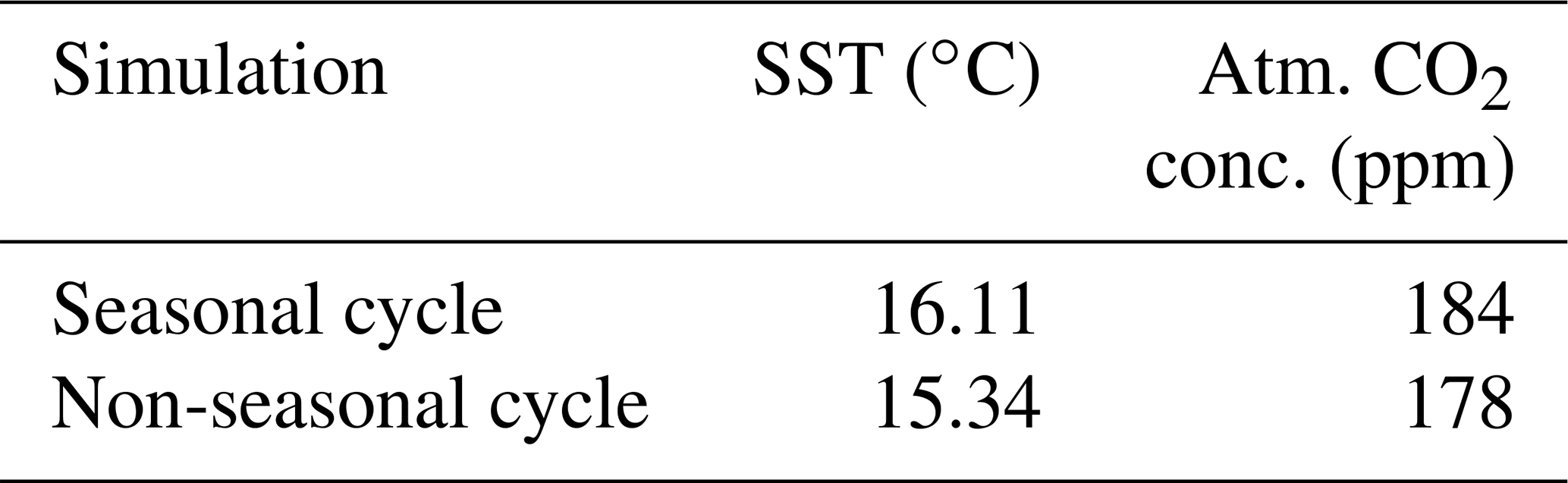
We compare two model simulations with phytoplankton light absorption. The model setups are similar except that we switched off the seasonal cycle in one simulation. Turning off the seasonal cycle decreases the mean annual SST by 0.77 ^∘C. Furthermore, the difference of atmospheric CO₂ concentration is 6 ppm. This difference is due to different SST and therefore different CO₂ solubility between these simulations. Our results without seasonality indicate that the difference of SST between BioLA and Bio is 0.14 ^∘C. Similar simulations have been conducted with a seasonal cycle, and the SST difference is 0.33 ^∘C (Asselot et al., 2021). The absence of a seasonal cycle reduces the difference of SST between the simulations with and without phytoplankton light absorption.

Table E1 Sea surface temperature (^∘C) and atmospheric CO₂ concentration (ppm) for simulations with and without a seasonal cycle.

Appendix F: Sea ice

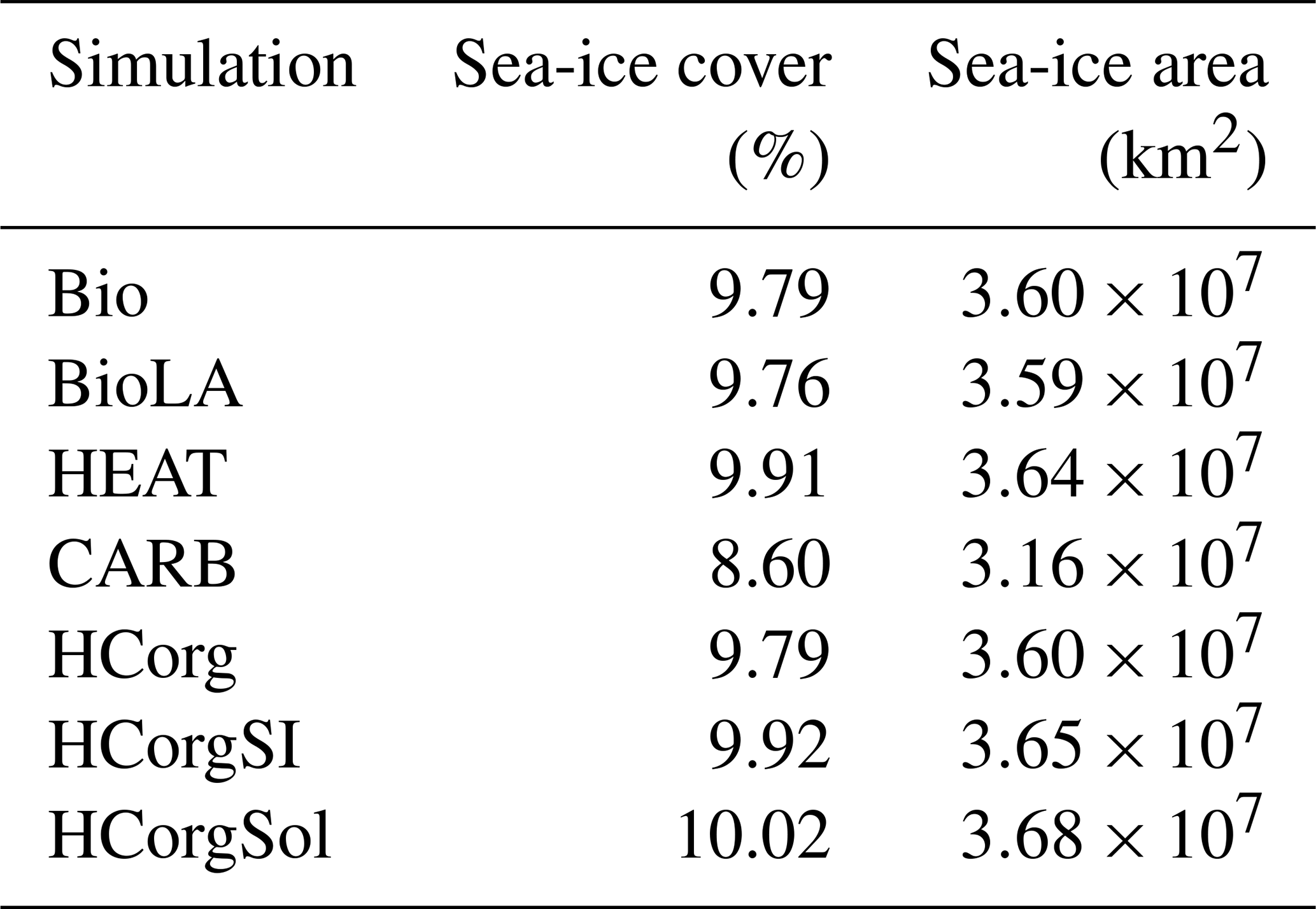
The global sea-ice cover and the global sea-ice area between the simulations HCorg and HCorgSI are identical, explaining their identical climate state. Moreover, the variation of sea ice between all simulations is small. The maximum global sea-ice cover change of 1.42 % occurs between the simulations CARB and HCorgSol.

Table F1 Global sea-ice cover (%) and global sea-ice area (km²) for the different simulations.

Appendix G: Precipitation

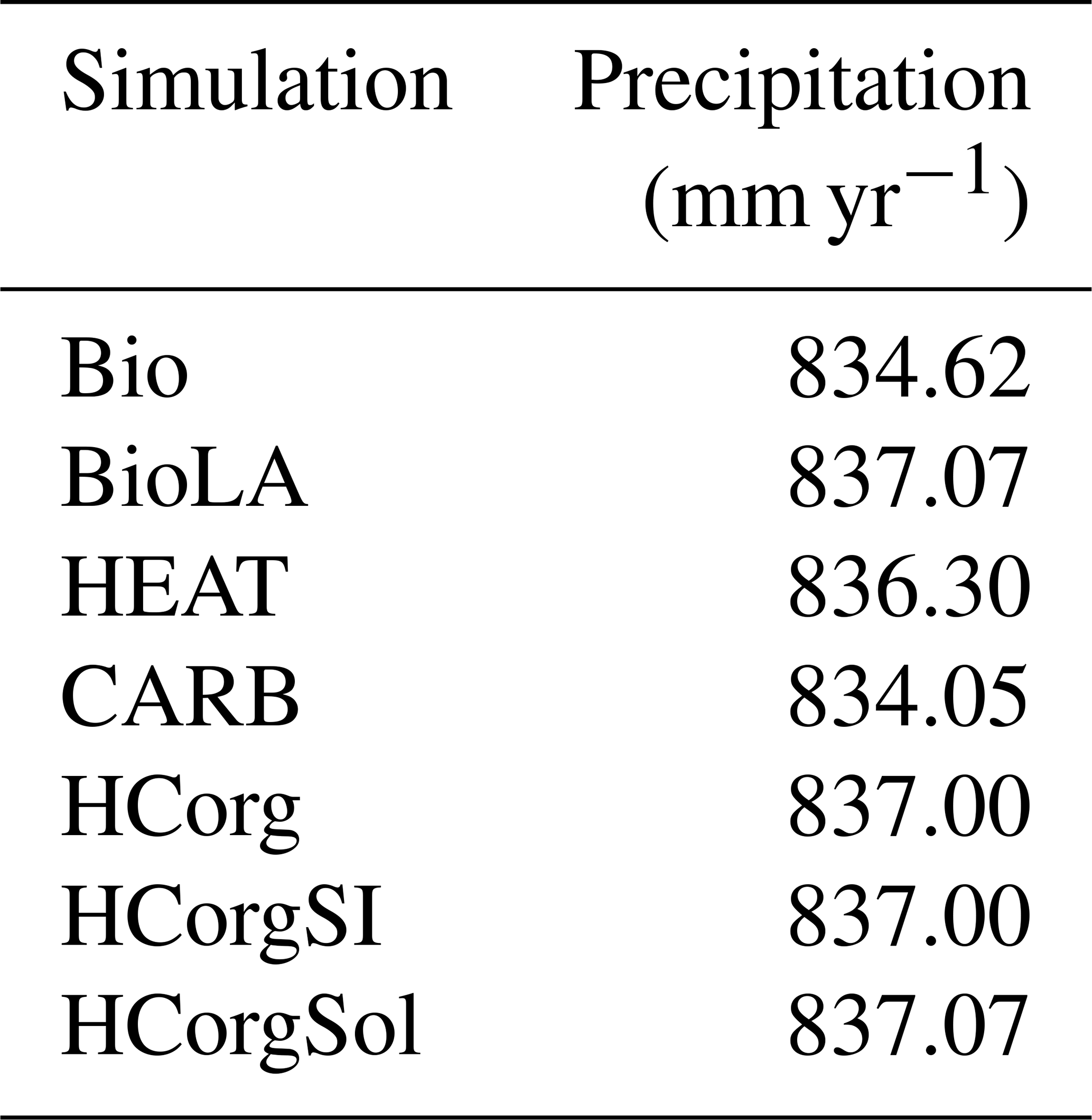
Slight fluctuations in precipitation are visible in Table G1. First of all, the precipitation between BioLA and HCorgSol are similar, and the same is true for the precipitation between HCorg and HCorgSI. The precipitation rate is the highest in the simulation BioLA due to the important specific humidity. In contrast, HEAT has a low specific humidity explaining the lowest precipitation rate for this simulation.

Table G1 Precipitation (mm yr⁻¹) for the different simulations.