Regional-scale phytoplankton dynamics and their association with glacier meltwater runoff in Svalbard

Arctic amplification of global warming has accelerated mass loss of Arctic land ice over the past decades and led to increased freshwater discharge into glacier fjords and adjacent seas. Glacier freshwater discharge is typically associated with high sediment load which limits the euphotic depth but may also aid to provide surface waters with essential nutrients, thus having counteracting effects on marine productivity. In situ observations from a few measured fjords across the Arctic indicate that glacier fjords dominated by marine-terminating glaciers are typically more productive than those with only land-terminating glaciers. Here we combine chlorophyll a from satellite ocean color, an indicator of phytoplankton biomass, with glacier meltwater runoff from climatic mass-balance modeling to establish a statistical model of summertime phytoplankton dynamics in Svalbard (mid-June to September). Statistical analysis reveals significant and positive spatiotemporal associations of chlorophyll a with glacier runoff for 7 out of 14 primary hydrological regions but only within 10 km distance from the shore. These seven regions consist predominantly of the major fjord systems of Svalbard. The adjacent land areas are characterized by a wide range of total glacier coverage (35.5 % to 81.2 %) and fraction of marine-terminating glacier area (40.2 % to 87.4 %). We find that an increase in specific glacier-runoff rate of 10 mm water equivalent per 8 d period raises summertime chlorophyll a concentrations by 5.2 % to 20.0 %, depending on the region. During the annual peak discharge we estimate that glacier runoff increases chlorophyll a by 13.1 % to 50.2 % compared to situations with no runoff. This suggests that glacier runoff is an important factor sustaining summertime phytoplankton production in Svalbard fjords, in line with findings from several fjords in Greenland. In contrast, for regions bordering open coasts, and beyond 10 km distance from the shore, we do not find significant associations of chlorophyll a with runoff. In these regions, physical ocean and sea-ice variables control chlorophyll a, pointing at the importance of a late sea-ice breakup in northern Svalbard, as well as the advection of Atlantic water masses along the West Spitsbergen Current for summertime phytoplankton dynamics. Our method allows for the investigation and monitoring of glacier-runoff effects on primary production throughout the summer season and is applicable on a pan-Arctic scale, thus complementing valuable but scarce in situ measurements in both space and time.

1 Introduction

The Arctic cryosphere is experiencing rapid transitions due to Arctic amplification of global warming. Climate change is reflected in changing oceanic and atmospheric circulation patterns, permafrost degradation, decline in sea-ice thickness and extent, and shrinking glaciers (IPCC, 2019; AMAP, 2017). Over the past few decades, glaciers and ice caps in the Arctic have retreated and lost mass at accelerating rates (e.g., Hugonnet et al., 2021), including glaciers in Svalbard (Schuler et al., 2020). A long-term trend of increased mass loss is also observed for the Greenland ice sheet despite a temporary slowdown of mass loss in 2013–2017 (IMBIE Team, 2019). Ice mass loss in the form of glacial meltwater runoff or frontal ablation, i.e., iceberg calving and submarine melt, constitutes a significant source of freshwater being discharged into glacial fjords and adjacent seas (Bamber et al., 2018). This glacier freshwater discharge has implications for the physical oceanographic conditions (Straneo and Cenedese, 2015; Carroll et al., 2017) and the biogeochemistry of water masses (Wadham et al., 2013; Hopwood et al., 2016), which affects the biological productivity in the fjords and the ocean (e.g., Juul-Pedersen et al., 2015; Meire et al., 2016; Hopwood et al., 2020).

Arctic marine ecosystems display strong seasonal cycles in productivity and functioning due to the pronounced seasonality of environmental variables such as solar radiation, sea-ice concentration, sea-surface temperature and salinity, as well as terrestrial freshwater input (Wassmann et al., 2020). Marine primary production, i.e., the generation of phytoplankton biomass, ultimately depends on the availability of light and the supply of essential, “limiting” nutrients (Sakshaug, 2004). Seasonal changes in any of these factors lead to periods of high or low primary production (Popova et al., 2010; Arrigo and van Dijken, 2015). A characteristic “phytoplankton spring bloom” follows the rapid increase in incoming solar radiation after the polar night, combined with high initial nutrient levels and the development of a weak stratification (Sakshaug, 2004; Tremblay et al., 2006). The persistence of sea ice, with or without snow cover, may delay the penetration of light into the water column and thus the phytoplankton spring bloom (Rysgaard and Nielsen, 2006; Song et al., 2021). Stratification during spring bloom is due to freshwater input mainly from melting of sea ice, as well as solar heating. Stratification ensures that the phytoplankton remains within the euphotic zone, i.e., the upper part of the water column where sufficient light is available for photosynthesis. Stratification favors primary production at an initial stage but also limits nutrient supply from intermediate-depth water (Tremblay et al., 2006, 2008). Nutrient depletion and increased grazing pressure by a growing zooplankton population terminate the spring bloom and lead to post-spring bloom minima in phytoplankton concentrations (Rysgaard et al., 1999; Calbet et al., 2011; Juul-Pedersen et al., 2015). New production of phytoplankton during summer requires a supply of limiting nutrients to the euphotic zone either by mobilization of nutrients from deeper water layers or input from external sources, such as dust storms (Prospero et al., 2012), coastal erosion and river discharge (Terhaar et al., 2021).

Recent studies have shown that tidewater glaciers sustain high primary production throughout summer in Greenland fjords and coastal waters (Juul-Pedersen et al., 2015; Arendt et al., 2016; Meire et al., 2016; Arrigo et al., 2017; Meire et al., 2017). In Godthåbsfjord, a sub-Arctic tidewater glacier fjord in southwest Greenland, Juul-Pedersen et al. (2015) observed a secondary peak in primary production, or “summer bloom”, that coincided with substantial runoff from the Greenland Ice Sheet. This summer bloom may be of similar magnitude or even exceed the spring bloom. Similar findings are available from Glacier Bay, Alaska (Etherington et al., 2007).

Glacial freshwater discharge enters the fjord or coastline either via pro-glacial rivers fed by runoff from land-terminating glaciers or via frontal ablation and runoff from marine-terminating glaciers (Bamber et al., 2018). These tidewater glaciers are typically highly crevassed so that most of the meltwater percolates into the glacier and is discharged subglacially at the glacier grounding line, where it is injected into the fjord at depth (Carroll et al., 2017). Glacier runoff can have counteracting effects on the productivity of Arctic fjords (e.g., Hopwood et al., 2020). Glacier runoff may be a direct source of nutrients to downstream ecosystems, for example bioavailable iron, nitrogen, phosphate or silicate (Hodson et al., 2005; Bhatia et al., 2013; Hawkings et al., 2015; Fransson et al., 2015; Meire et al., 2016; Dubnick et al., 2017; Milner et al., 2017; Hopwood et al., 2018). However, glacial meltwater is generally characterized by low nutrient concentrations in comparison with the ambient seawater (Halbach et al., 2019; Cantoni et al., 2020; Hopwood et al., 2020). In addition, glacier runoff is typically associated with high sediment loads (Dowdeswell et al., 2015; Schild et al., 2018) which limit the light penetration into the water column and thereby the extent of the euphotic zone. In Svalbard, the euphotic depth may vary from less than about 0.3 m within subglacial discharge plumes near glacier calving fronts to more than 30 m in the outer parts of the fjords (Svendsen et al., 2002; Piquet et al., 2014; Halbach et al., 2019; McGovern et al., 2020). Poor light conditions near glacier fronts thus limit primary production (Zajaczkowski and Wlodarska-Kowalczuk, 2007; Svendsen et al., 2002; Calleja et al., 2017; Hegseth et al., 2019). With increasing distance from the glaciers or pro-glacial river, light conditions become more favorable as progressively more sediments settle out. Phytoplankton growth will then mainly depend on the supply of limiting nutrients to the euphotic zone (Halbach et al., 2019; Hopwood et al., 2020).

The effect of glacier runoff on vertical mixing provides an indirect mechanisms by which to fertilize the marine ecosystem. Subglacial discharge drives buoyant upwelling of plumes near the calving front of tidewater glaciers, which leads to the entrainment of large volumes of ambient seawater from all depth levels (Carroll et al., 2017), thereby supplying nutrient-depleted surface layers with nutrients from nutrient-rich deep water layers (Meire et al., 2017; Kanna et al., 2018; Hopwood et al., 2020). A study by Hopwood et al. (2018) suggests that this “nutrient pump” may provide the euphotic zone with 2 orders of magnitudes more nutrients than what is directly supplied by the glacial meltwater. Glacier runoff may also enhance the general estuarine circulation within fjords and embayments, which is considered to have positive effects on biological productivity (Rysgaard et al., 2003; Juul-Pedersen et al., 2015; Meire et al., 2016). Down-fjord katabatic winds facilitate the export of brackish/low-density surface water out of the fjord, which leads to a compensating return flow of nutrient-rich saline water at depth (Svendsen et al., 2002; Cottier et al., 2010; Straneo and Cenedese, 2015; Spall et al., 2017; Sundfjord et al., 2017). In either case, positive effects of glacier runoff on primary productivity are expected to occur only where suspended particles have settled deeper into the water column and light conditions in surface waters become more favorable (Etherington et al., 2007; Lydersen et al., 2014; Halbach et al., 2019).

In situ studies across the Arctic show a large variability in marine primary production in response to glacier runoff for individual fjord systems due to distinct fjord geometry, the presence and depth of an entry sill, glacier configuration of marine- and land-terminating glaciers, and oceanographic conditions and climatic setting (e.g., Hopwood et al., 2018, 2020). Glacial fjords dominated by tidewater glaciers appear to have a higher productivity than those dominated by land-terminating glaciers (Meire et al., 2017; Hopwood et al., 2020), underpinning the importance of subglacial upwelling. A study by Holding et al. (2019) revealed low primary production in a northeast Greenland fjord dominated by land-terminating glaciers as glacier runoff limited light availability and enhanced stratification. Nevertheless, this low productivity was sustained throughout the ice-free season, well into fall. In Svalbard, glacier runoff is known to affect the distribution and species composition of phytoplankton (Piquet et al., 2014; van de Poll et al., 2018), but it is a matter of debate whether or not glacier runoff facilitates higher productivity during summer (Halbach et al., 2019).

The current knowledge about the impacts of glacier runoff on marine primary production is largely based on in situ observations. While providing valuable information about the measured variables at specific locations, in situ observations are often limited in space and time, typically capturing a snapshot of the situation at the surveyed site. This highlights the need for innovative long-term monitoring programs of proglacial marine ecosystems (Straneo et al., 2019). In addition, efforts should be taken to upscale local in situ observations in space and time. This can be achieved by the application of modeling approaches and/or satellite remote sensing.

This study aims to investigate the overall effects of glacier runoff on phytoplankton dynamics and marine primary productivity in Svalbard, focusing on a regional rather than local scale. We utilize a 10-year time series of glacier runoff from high-resolution climatic mass balance simulations of all glaciers in Svalbard for the time period 2003–2013 (Aas et al., 2016) and chlorophyll a concentrations from satellite ocean color, an indicator of phytoplankton biomass (Moses et al., 2009; Matrai et al., 2013; Kahru et al., 2014; Lee et al., 2015). Chlorophyll a products and other physical ocean variables, including sea-surface temperature (SST) and sea-ice fraction (SIF), are available through the Copernicus Marine Service (CMEMS). We use a statistical model to identify significant associations of chlorophyll a with runoff while accounting for the potentially confounding effects of physical ocean and sea-ice variables that may covary with runoff. We focus on the summer melt period, from mid-June to September, anticipating that this period follows the termination of the spring bloom. Specifically, we investigate whether there are significant associations between runoff and chlorophyll a in coastal waters around Svalbard, and if there are spatial variations in association strength, e.g., with respect to regional characteristics or distance to coast.

2 Research region

The Svalbard archipelago in the Eurasian Arctic is bordered by the Barents Sea to the east, the Greenland Sea to the west and the Arctic Ocean to the north (Fig. 1). The climate in Svalbard is relatively warm, given its high Arctic location. This is due to the West Spitsbergen Current (WSC), an extension of the North Atlantic Current, which transports warm Atlantic Water up north along the West Spitsbergen Shelf (Svendsen et al., 2002; Walczowski and Piechura, 2011, Fig. 1a). The eastern side of Svalbard is dominated by the East Spitsbergen Current (ESC), which transports cold Arctic Water clockwise around the southern tip of Spitsbergen (Loeng, 1991; Svendsen et al., 2002). It continues northwards on the West Spitsbergen Shelf, forming a coastal current which is subsequently freshened by the export of brackish surface water from the fjords (Svendsen et al., 2002; Nilsen et al., 2016, Fig. 1a).

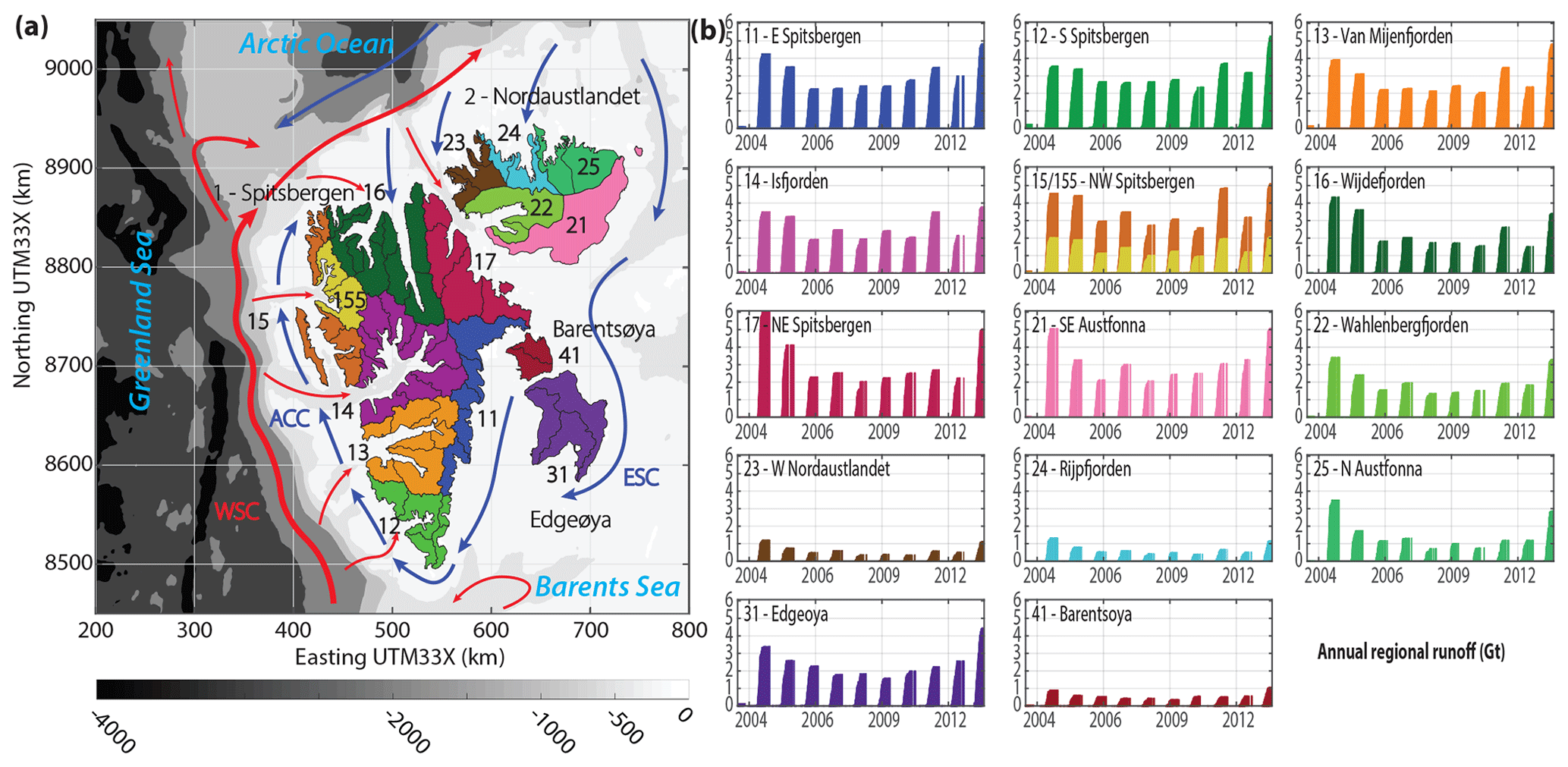
Figure 1 (a) Map of Svalbard with 14 primary hydrological regions (two-digit ID number) and one subregion (155 – Kongsfjorden and 156 – Krossfjorden) shown in different colors. Black outlines indicate secondary hydrological regions. The bathymetry is shown in shades of gray (IBCAO dataset). Adjacent seas and major currents are plotted according to Svendsen et al. (2002) and Hop et al. (2019) in which the red arrows delineates the West Spitsbergen Current (WSC) and pathways of Atlantic Water, and the blue arrows the Arctic Coastal Current (ACC), originating as East Spitsbergen Current (ESC), and other pathways of Arctic Water. (b) Regional time series of annual cumulative glacier runoff extracted from climatic mass-balance simulations by Aas et al. (2016).

From 1971 to 2017, Svalbard has experienced strong atmospheric warming by 3–5 ^∘C (Hanssen-Bauer et al., 2019), evident in all seasons but most pronounced during winter and spring (Nordli et al., 2014). Strong atmospheric warming is attributed to a general decline in sea ice and an increase in sea-surface temperatures (Isaksen et al., 2016). Climate projections under medium to high emission scenarios indicate that air temperatures may rise by 7–10 ^∘C by 2071–2100, as compared to 1971–2000, which may lead to a 5-fold increase in glacier mass loss (Hanssen-Bauer et al., 2019).

Glaciers and ice caps cover 57 % (34 000 km²) of the total land area in Svalbard. Tidewater glaciers drain 68 % of the glacierized area and have a combined total calving-front length of ∼740 km (Nuth et al., 2013). The degree of glacier coverage and the size of individual glaciers reflect the general climatic gradient across Svalbard. Glaciers in the southern and western parts, characterized by relatively warm atmospheric and oceanic conditions, are generally smaller than glaciers in the northeastern parts of Svalbard, where colder climatic conditions prevail. Consequently, the total glacier coverage is lower in the southern and western parts, with a minimum in the dry central parts of Spitsbergen (Nuth et al., 2013). Overall, glaciers in Svalbard have been loosing mass since the 1960s, with a pronounced increase in mass loss since the 2000s (Schuler et al., 2020). A compilation of available mass balance assessments for the period 2000–2019 reveals a total mass balance of $-\mathrm{8}\pm \mathrm{6}$ Gt a⁻¹, of which $-\mathrm{7}\pm \mathrm{4}$ Gt a⁻¹ are attributed to the climatic mass balance and $-\mathrm{2}\pm \mathrm{7}$ Gt a⁻¹ to the poorly constrained frontal ablation, i.e., iceberg calving and submarine melt (Schuler et al., 2020). The climatic mass balance simulation by Aas et al. (2016), from which we extract glacier runoff, is included in this reconciled mass balance estimate. For the period 2003–2013, Aas et al. (2016) found a mean annual mass balance of about −8.7 Gt, which is well within the error margins of the consensus estimate by Schuler et al. (2020).

Fjords in Svalbard are affected by terrestrial freshwater discharge, on the one hand, and the exchange of water masses with the adjacent shelf, on the other hand (Svendsen et al., 2002; Cottier et al., 2005; Nilsen et al., 2016; Sundfjord et al., 2017). Glacier ablation constitutes the major component of the terrestrial freshwater discharge into Svalbard fjords (Pramanik et al., 2018; van Pelt et al., 2019). During the summer melt season, glacier runoff enters the fjord in the form of surface runoff and subglacial discharge, in addition to iceberg calving and submarine melt. This freshwater mixes with ambient fjord water to form a layer of brackish surface waters, its thickness typically decreasing from the head towards the mouth of the fjord (Svendsen et al., 2002). The exchange of water masses between the fjords and the shelf depends on stratification and wind-stress, as well as the presence or absence of a topographic barrier, e.g., in the form of a shallow sill at the fjord mouth (Cottier et al., 2010). The dominating wind field in Svalbard fjords is down-fjord due to katabatic winds and orographic steering of the large-scale wind field (Svendsen et al., 2002; Cottier et al., 2005). This drives brackish surface water out of the fjord and a compensating inflow of Atlantic Water from the shelf, thereby stimulating estuarine circulation and vertical mixing of water masses (Svendsen et al., 2002; Cottier et al., 2010; Sundfjord et al., 2017). In addition to wind-stress, the circulation in broad fjords, such as found in Svalbard, is influenced by rotational dynamics or “Coriolis” effects (Svendsen et al., 2002; Cottier et al., 2010). Changes in atmospheric circulation patterns since the early 2000s have caused repeated overflow of the WSC onto the West Spitsbergen Shelf and inflow of warm saline Atlantic Water into some of the major fjords, with implications for water mass composition and heat content, significantly reducing sea-ice production during wintertime (Cottier et al., 2007; Nilsen et al., 2016).

For our regional-scale assessment of glacier runoff effects on phytoplankton dynamics and marine primary production, we consider 14 primary drainage basins or hydrological regions of Svalbard (Fig. 1a), following the most recent Svalbard glacier inventory (Nuth et al., 2013; König et al., 2014). The identification system follows Hagen et al. (1993), in which the first digit represents one out of five major areas: (1) Spitsbergen, (2) Nordaustlandet, (3) Barentsøya, (4) Edgeøya and (5) Kvitøya, the latter of which is not included in this study. The second and third digits indicate the primary and secondary drainage basins, respectively. For each hydrological region, we distinguish between different marine zones, defined by their distances from the coast, namely 0 to 10, 10 to 20 and 20 to 50 km. The innermost zone contains most of the fjords, which typically have a width of less than 20 km. The outer regions beyond 10 km distance from the coast extend into the open ocean. Along the western and northern side of Spitsbergen, the 50 km offshore distance contour line corresponds approximately with the shelf edge. In addition to the primary hydrological regions, we consider one subregion near the research hub of Ny-Ålesund in northeast Spitsbergen (15). The Kongsfjorden–Krossfjorden system consists of two secondary drainage basins, Kongsfjorden (155) and Krossfjorden (156), and serves as a key site for interdisciplinary studies on glacier–ocean interactions, focusing on physical oceanographic conditions in response to glacier runoff (Svendsen et al., 2002; Cottier et al., 2005; Sundfjord et al., 2017; Torsvik et al., 2019) and their implications for the marine ecosystem (Lydersen et al., 2014; Piquet et al., 2014; Calleja et al., 2017; Halbach et al., 2019; Hegseth et al., 2019).

3 Material and methods

3.1 Climatic glacier mass balance and meltwater runoff

We extracted regional glacier meltwater runoff from a 10-year simulation of the climatic mass balance of all glaciers in Svalbard, later referred to as glacier runoff or simply runoff. The coupled atmosphere–glacier model was run over the time period September 2003 to September 2013 (Aas et al., 2016). The glacier model computes the climatic mass balance (CMB), i.e., the mass fluxes at the surface of the glacier mainly due to deposition of snow during the accumulation season (typically October to May) and surface melt followed by runoff during the ablation season (typically June to September). The CMB model is implemented into the Weather Research and Forecasting model (WRF), which provides precipitation and other meteorological variables to the CMB model that are required to compute the climatic mass balance, considering the surface energy balance. WRF is a mesoscale atmospheric model (Skamarock and Klemp, 2008). In Svalbard it has been applied to study boundary layer processes (Kilpelainen et al., 2011, 2012) and atmosphere–land interactions over both tundra (Aas et al., 2015) and glaciers (Claremar et al., 2012; Aas et al., 2016). Coupled model simulations were run over all of Svalbard at 3 km horizontal resolution using sea-surface temperature and sea-ice concentration from the Operational Sea Surface Temperature and Sea Ice Analysis (OSTIA) and ERA-Interim climate reanalysis data as boundary conditions. Results were validated against field observations of meteorological conditions and in situ measurements of snow accumulation and surface-mass balance across the archipelago (Aas et al., 2016).

For grid cells covered by glaciers, the land-surface scheme of WRF was replaced by a modified version of the CMB model by Mölg et al. (2008, 2009), specifically adjusted for Arctic conditions (Aas et al., 2016). The model simulates the development of multi-year snowpacks and their transition into firn and ice. The CMB model employs meteorological variables generated by WRF, near-surface temperature, humidity, pressure, wind speed and incoming radiation to solve the surface energy balance and determine the energy available for melt. Solid precipitation and surface and subsurface melt then yield the column-specific mass balance over 17 layers down to 20 m depth. Variables are computed at a 20 s temporal resolution and are then aggregated into daily values.

Daily glacier runoff is determined as the difference between a production and a retention term of liquid water at or near the glacier surface. Production of liquid water is given as the sum of surface melt, internal melt and rain (liquid precipitation). Meltwater retention is the sum of internal refreezing within the snow and firn, superimposed ice formation, i.e., water refreezing on top of impermeable ice, and liquid water storage or, more precisely, the change in liquid water content. Meltwater production is highest at lower glacier elevation but not restricted to the ablation area. At higher elevation within the accumulation area, locally produced meltwater may be stored in the snow and firn column, thus reducing or preventing runoff. Runoff from each region is first computed in absolute terms (Gt; Fig. 1b) and then normalized by the associated area of the sea (km²), up to a defined distance from the coast (10, 20 or 50 km). This yields specific runoff received by the sea in terms of millimeter water equivalent (RUNOFF, in $\mathrm{mm}\mathrm{w}.\mathrm{e}.$), i.e., the same units as used for expressing precipitation amounts or specific glacier mass balance. Note that our CMB model does not include a scheme for transport and routing of meltwater. The exact location of meltwater input to the fjords and ocean is therefore unknown. However, this does not compromise our regional-scale analysis, in which all glacier runoff generated within a primary hydrological region drains into the same associated fjord system or adjacent sea. Similarly, the glacier model does not distinguish between surface runoff and subglacial discharge.

Mean specific climatic net mass balance of Svalbard glaciers for the period 2003–2013 was negative, −257 $\mathrm{mm}\mathrm{w}.\mathrm{e}.{\mathrm{yr}}^{-\mathrm{1}}$, which corresponds to a mean annual mass loss of about 8.7 Gt (Aas et al., 2016). Interannual variability in climatic mass balance is large and dominated by a high variability in summer ablation. This is closely reflected in the annual cumulative runoff curves for the various hydrological regions (Fig. 1b). Regional glacier runoff is a function of the total regional glacier area and region-specific ablation. On average, Svalbard-wide specific glacier ablation and thus total annual glacier runoff amounted to 919 $\mathrm{mm}\mathrm{w}.\mathrm{e}.$ and 31.2 Gt, respectively, with a minimum in summer 2008 (673 $\mathrm{mm}\mathrm{w}.\mathrm{e}.$; 22.9 Gt) and a maximum in summer 2013 (1508 $\mathrm{mm}\mathrm{w}.\mathrm{e}.$; 51.3 Gt).

3.2 Ocean data

Chlorophyll a concentration (CHL, in mg m⁻³) in near-surface waters was quantified using satellite data from the European Space Agency (ESA) Ocean Colour Climate Change Initiative (CCI). We used Arctic reprocessed version L4 data obtained from the Copernicus Marine Environment Monitoring Service (CMEMS), providing 8 d means of merged, bias-corrected remote sensing reflectance at 1 km resolution from 1998 to 2014 (see “Data availability” section below). This product merges reflectance data from SeaWiFS, MODIS-Aqua and MERIS sensors by realigning the spectra to those of the SeaWiFS sensor. Chlorophyll a is estimated from the OC5ci algorithm, which is a combination of two ocean color algorithms for chlorophyll retrieval. The first is developed for clear waters in the open ocean, where ocean color is dominated by chlorophyll a, i.e., the green pigment contained in phytoplankton biomass (case-1 waters; CI; Hu et al., 2012; Sathyendranath et al., 2012). The second is optimized for optically complex coastal waters, influenced by terrestrial runoff and hence suspended sediments and colored dissolved organic matter (case-2 waters; OC5; Gohin et al., 2008). For Svalbard, chlorophyll a observations are typically limited to late March to early September each year.

As key environmental variables other than RUNOFF we consider sea-surface temperature (SST, in ^∘C), mixed-layer depth, a measure of stratification (MLD, in m) and sea-ice fraction (SIF, [0 1]). Daily means of these variables at 12.5 km resolution for the years 1998–2014 were extracted from the TOPAZ4 Arctic Ocean Physics Reanalysis (version V0.3) obtained from CMEMS. The TOPAZ4 reanalysis uses the Hybrid Coordinate Ocean Model (HYCOM), an operational general ocean-circulation model that assimilates remotely sensed sea level anomalies, sea-surface temperature, sea-ice concentration and Lagrangian sea-ice velocities (winter only, since 2002), as well as temperature and salinity profiles from Argo floats using a 100-member deterministic version of the ensemble Kalman filter (Sakov et al., 2012). A rigorous quality assessment of the TOPAZ4 dataset can be found in Xie et al. (2017).

3.3 Statistical analysis

All data (CHL, RUNOFF, SST, MLD, SIF) were first aggregated into regional time series with the same 8 d temporal resolution as CHL. For each of the 14 hydrological regions (plus one subregion), we constructed three time series of different spatial scale and near-shore influence: 0–10, 10–20 and 20–50 km distance from land. The main emphasis is on 0–10 km from land as this covers the major fjord systems where we expect the largest potential RUNOFF effects.

To test if associations between RUNOFF and CHL were statistically significant we restricted the data to late summer (13 June to 15 October, i.e., annual 8 d periods 21 to 36). This period includes the main glacier summer melt period (mid-June to September) and is expected to start after termination of the phytoplankton spring bloom. For each region and spatial scale we considered the following generic model:

$$\begin{array}{}\text{(1)}& {\displaystyle }{\displaystyle }\log \left({\text{CHL}}_{r,t}\right)={\mathit{\alpha }}_r+{\mathit{\beta }}_r\cdot \log \left({\text{CHL}}_{r,t-\mathrm{1}}\right)+{\mathit{c}}_r\cdot {\mathit{e}}_{r,t}+{\mathit{\epsilon }}_{r,t}.\end{array}$$

Here log (CHL_r,t) is the natural logarithm of CHL in region r (and a given distance interval from land) at time t, α_r is the intercept, β_r is the auto-regressive effect of CHL in the previous time step, c_r is a row vector with coefficients for environmental effects, e_r,t is a column vector with the environmental covariate values, ε_r,t is a normally and independently distributed error term with variance ${{\mathit{\sigma }}_r}^{\mathrm{2}}/n_{r,t}$, and n_r,t is the number of CHL observations that were averaged to calculate CHL_r,t. By weighting the error variance with sample size, region–time combinations with few CHL observations, e.g., due to cloud cover, have less influence on results than region–time combinations with many observations.

To determine which environmental variables to include for each region, we used a two-step approach. We first found the best model without RUNOFF, using data for all years 1998–2014 (whereas RUNOFF was only available from September 2003 to September 2013). Variables were selected stepwise by adding terms if it led to a lower value of the information criterion AIC_C, i.e., the Akaike information criterion corrected for small sample size (Hurvich and Tsai, 1989). The AIC_C helps to find the best trade-off between the goodness-of-fit of a model and the simplicity of the model; a model with lower AIC_C is preferred over a model with higher AIC_C. Terms only marginally significant (P>0.05) were removed from the model. Nine candidate variables were considered at this step: (1) SST_r,t, (2) ${\text{SST}}_{r,t-\mathrm{1}}$, (3) ${\text{SST}}_{\mathrm{d}t}={\text{SST}}_{r,t}-{\text{SST}}_{r,t-\mathrm{1}}$, (4) log (MLD_r,t), (5) $\log \left({\text{MLD}}_{r,t-\mathrm{1}}\right)$, (6) $\log \left({\text{MLD}}_{\mathrm{d}t}\right)=\log \left({\text{MLD}}_{r,t}\right)-\log \left({\text{MLD}}_{r,t-\mathrm{1}}\right)$, (7) SIF_r,t, (8) ${\text{SIF}}_{r,t-\mathrm{1}}$, and (9) ${\text{SIF}}_{\mathrm{d}t}={\text{SIF}}_{r,t}-{\text{SIF}}_{r,t-\mathrm{1}}$. The difference variables SST_dt and log (MLD_dt) were included as possible indicators of mixing of deeper nutrient-rich water masses into the surface layer. The difference variable SIF_dt was included as an indicator of the sea-ice breakup and the associated increase in light levels in the water column. We then added RUNOFF and RUNOFF_t−1 to the model selected in the first step but only if leading to lower AIC_C (for the reduced period with RUNOFF data) and only if the association was significant at P<0.05. A summary of all regional models, including model equations, parameter estimates with standard errors and statistical significance, can be found in the Appendix (Tables A1–A3).

To assess if key model assumptions were met, we checked if residuals were independent and approximately normally distributed. Specifically, Pearson residuals (i.e., residuals standardized to unit standard deviation) from the final model for each region were explored for independence by plotting the autocorrelation function and the partial autocorrelation function and for approximate normality by plotting quantile-quantile normal plots. The residuals from the final model for each region were uncorrelated in time and approximately normally distributed, with a possible exception of region 22 in the analysis for 0–10 km from the coast, which showed indications of unequal variance. We also checked if results were strongly influenced by a few outlying observations. Outliers were identified as residuals more than 3.3× standard deviations away from zero, which is expected to occur by chance for 1 out of 1000 normally distributed cases, i.e., for about 2–3 out of the >2000 observations analyzed. Within 10 km distance from the coast, 13 residuals distributed among 10 regions were identified as outliers. A similar number of outliers existed for the other distances from the coast. If outliers were identified, we refitted the model excluding the outliers. Since the removal of outliers had little influence on parameter estimates for RUNOFF effects, we kept them in the present model (all the coefficients remained statistically significant at P<0.05). All statistical analyses were performed using the R programming environment (R Core Team R., 2016).

4 Results

We first present regional associations of CHL with glacier runoff (Sect. 4.1) before moving on to associations with physical-ocean and sea-ice variables (Sect. 4.2). Interpretation of these results will be discussed in the following section (Sect. 5). Our statistical model identifies the environmental variables that best explain the observed regional summertime CHL (Figs. 2 and A1–A3). The model considers instantaneous and delayed associations of CHL with a set of predictor variables, based on variable values during the current and previous 8 d time step marked by an index “t” and “t−1”, respectively. In addition, the model inspects associations of CHL with the rate of change in selected environmental variables (index “dt”). Note that the associations that we hereafter discuss are partial effects, i.e., the association of CHL with each predictor variable, while accounting for all other predictor variables selected in the model. Specifically, the statistical model estimates the joint effects of all selected predictor variables on CHL, and the partial effect of a variable represents the expected effect of that variable if all other variables are kept constant. As a model control run, we test the auto-correlation of CHL in the current and previous time step. This “null model” reveals a significant positive association in all regions regardless of distance from the coast, as expected (Figs. 2a and A1–A3). In other words, if there is high CHL in the previous 8 d time step, then it is likely that CHL will also be high in the present time step.

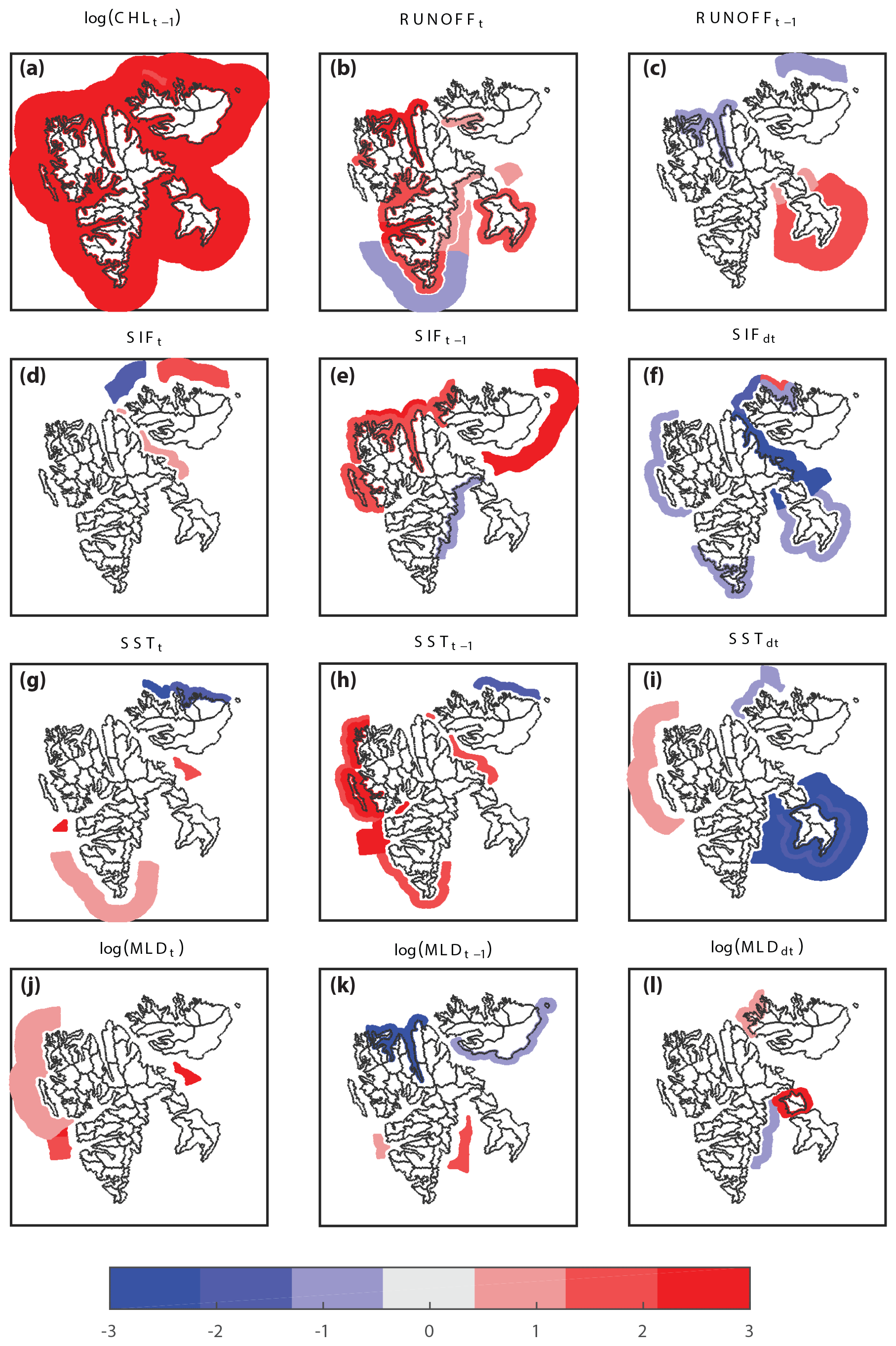
Figure 2 Regional significance of environmental variables and their association with the predicted chlorophyll a concentrations within 0–10, 10–20 and 20–50 km from the coast: CHL during previous 8 d period (a); glacier runoff, RUNOFF, during the current and previous 8 d period (b, c); current, previous and change in sea-ice fraction, SIF (d–f; denoted by index t, t−1 and dt); sea-surface temperature, SST (g–i); and mixed-layer depth, MLD (j–l). Positive associations are indicated by red shades and negative by blue. The intensity of the color showing the level of significance of the association (1: P<0.05; 2: P<0.01; 3: P<0.001).

4.1 Association of summertime chlorophyll a with glacier runoff

We find significant positive associations of CHL with RUNOFF in half of the primary hydrological regions (7 out of 14), namely eastern Spitsbergen (Region 11), southern Spitsbergen (12), Van Mijen- and Van Keulenfjorden (13), Isfjorden (14), Wijde- and Woodfjorden (16), and Wahlenbergfjorden (22) in Nordaustlandet and Edgeøya (31) in southeast Svalbard (Figs. 2 and A1). A positive association also exists for the subregion of Kongsfjorden–Krossfjorden (155), whereas no significant association exists for northwest Spitsbergen (15) as a whole. Positive associations are mainly restricted to within 10 km distance from the coast, indicating that the RUNOFF effect on CHL is mainly limited to within the fjords. Fjords in Svalbard have a maximum width of typically less than 20 km and are thus entirely covered by this range. Beyond 10 km distance from the coast, as well as for regions characterized by open coastal conditions, the significant positive association of CHL with RUNOFF vanishes (Figs. 2b, A2 and A3). At 10–20 km, there is no significant association, while at 20–50 km there is a weak negative association for southern Spitsbergen (12) and a weak positive association for eastern Spitsbergen (11) and Barentsøya (41). The latter regions all border Storfjorden, which forms a large, 40–80 km wide embayment between eastern Spitsbergen to the west and Barentsøya and Edgeøya to the east. There are only a few delayed associations of CHL with RUNOFF (Fig. 2c). For Edgeøya (31) a positive association is present at 10–50 km, in addition to the instantaneous response within 10 km distance from the coast (Fig. 2b). For neighboring Barentsøya (41) a weak positive association exists for the 10–20 km zone. CHL shows a negative delayed association with RUNOFF at 0–10 km for Wijdefjorden (16) and within 20–50 km off northeast Nordaustlandet (25).

Table 1 Glacier configuration and runoff characteristics for primary hydrological regions of Svalbard, including subregion Kongsfjorden–Krossfjorden.

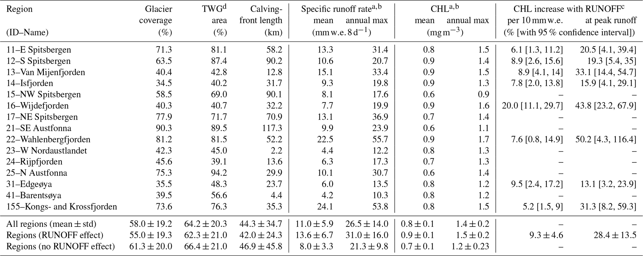
^a Specific runoff rate, CHL and CHL increase are based on marine area within 10 km from the coast. ^b Mean and mean annual maximum values are derived from annual 8 d periods 21–36 during 10 subsequent summers 2004–2013. ^c Mean chlorophyll a increase per 10 $\mathrm{mm}\mathrm{w}.\mathrm{e}.\mathrm{8}{\mathrm{d}}^{-\mathrm{1}}$ and at annual maximum runoff. Numbers in squared brackets provide the plausible range at 95 % confidence interval. ^d Glacier area drained through tidewater glaciers (TWG area).

We find that regions that display significant positive associations between CHL and RUNOFF within 10 km distance from the coast have a 26 % higher mean summertime chlorophyll a content and a 19 % higher mean annual maximum chlorophyll a content than regions without such associations (Table 1). Our statistical model suggests that an increase in specific runoff of 10 $\mathrm{mm}\mathrm{w}.\mathrm{e}.\mathrm{8}{\mathrm{d}}^{-\mathrm{1}}$ raises summertime chlorophyll a concentrations in these regions by 5.2 % to 20.0 %, or 9.3 % on average, with a standard deviation of 4.6 % (Table 1). During the annual peak discharge we estimate that runoff increases chlorophyll a by 13.1 % to 50.2 % or 28.4±13.5 % on average, compared to situations with no runoff.

4.2 Association of summertime chlorophyll a with physical ocean and sea-ice variables

There are both negative and positive associations of CHL with the physical ocean and sea-ice variables, although only for a limited number of regions. Concerning sea-ice variables, the current sea-ice fraction (SIF) has little association with CHL (Fig. 2d). However, there is a delayed positive association of CHL with SIF in northern Svalbard, mainly within 10 km from the coast (regions 15, 16, 23; Fig. 2e) but also 10–20 km (16) and 20–50 km (21), while CHL is negatively associated with a change in SIF at 0–10 and 10–20 km (regions 12, 15, 17, 21, 24, 31, 41; Fig. 2f).

Moving on to sea-surface temperature (SST), current SST has a few positive associations at 20–50 km distance from the shore (regions 12, 14 and 17) and negative associations north of Nordaustlandet at 0–10 and 10–20 km distance from the coast (24, 25; Fig. 2g). There is a positive delayed association of CHL and SST along the entire west coast of Spitsbergen at 0–10 and/or 10–20 km distance from the coast (12, 13, 14, 15; Fig. 2h), as well as in Hinlopen Strait off northeast Spitsbergen (17). There is a negative instantaneous association of CHL with SST north of Nordaustlandet (25). The association of CHL with a change in SST is negative all around Edgeøya (31) and Barentsøya (41), as well as western Nordaustlandet (23), and weakly positive in the outer region of northeast Spitsbergen (17) at 20–50 km distance from the coast (Fig. 2i).

Mixed-layer depth shows some positive association with CHL at the outer regions along the west coast of Spitsbergen (13, 14, 15) and Hinlopen (17; Fig. 2j). The delayed association between CHL and MLD is negative in two northern regions (16, 21) within 10 km from the coast and positive at 10–20 and 20–50 km for Isfjorden (14) and eastern Spitsbergen (11), respectively (Fig. 2k). The change in MLD has a few both positive and negative associations (Fig. 2l).

5 Discussion

We first discuss the observed associations of summertime CHL with the environmental variables and provide physical and biological explanations. We start with the associations of summertime CHL with RUNOFF (Sect. 5.1) before moving on to ocean and sea-ice variables which point at the effect of persistent sea-ice coverage and the influence of the West Spitsbergen Current (Sect. 5.2). We then describe the seasonal evolution of chlorophyll a in relation to environmental variables (Sect. 5.3). Finally, we discuss challenges related to the use of remotely sensed chlorophyll a as a proxy of phytoplankton biomass (Sect. 5.4).

5.1 Glacier-runoff effects on marine primary production

Our study suggests that the overall effect of glacier runoff on marine primary production is positive for 7 out of 14 hydrological regions in Svalbard. These regions represent the major fjord systems rather than coastal regions. Positive association is generally restricted to within 10 km distance from the coast; i.e. it does not extend far outside the fjords and onto the shelf. The primary hydrological regions have highly variable glacier coverage, ranging from 34.5 % for Isfjorden in central Spitsbergen to 90.3 % for southeast Austfonna on Nordaustlandet (Table 1). For regions which display significant and positive associations between CHL and RUNOFF, glacier characteristics in terms of glacier coverage, glacier area drained by tidewater glaciers and total calving-front length are on average ∼10 % smaller compared to regions without associations between CHL and RUNOFF. Regions which display significant and positive associations between CHL and RUNOFF are also characterized by a highly variable fraction of tidewater glacier-drained area, ranging from 40.2 % for Isfjorden to 87.4 % for southern Spitsbergen, with a regional mean of 62.3±21.0 %. This is slightly less than the corresponding mean value of 66.4±21.0 % in the other regions. Mean specific runoff rates per marine area within 10 km distance from the coast range from 4.2 $\mathrm{mm}\mathrm{w}.\mathrm{e}.\mathrm{8}{\mathrm{d}}^{-\mathrm{1}}$ for Barentsøya to 24.2 $\mathrm{mm}\mathrm{w}.\mathrm{e}.\mathrm{8}{\mathrm{d}}^{-\mathrm{1}}$ for Kongsfjorden–Krossfjorden (Table 1). Despite the slightly smaller average glacier coverage, regions with RUNOFF effect on CHL have higher specific runoff rates that exceed those in the other regions by 46 % and 69 % for mean specific runoff rates and specific mean annual peak runoff rates, respectively.

Field observations across the Arctic show that glacial fjords dominated by tidewater glaciers have generally higher productivity than those dominated by land-terminating glaciers (Hopwood et al., 2020). Runoff from marine-terminating glaciers is generally thought to enhance marine primary production through buoyant upwelling of subglacial discharge plumes (e.g., Kanna et al., 2018), whereas runoff from land-terminating glaciers is thought to limit primary production, as a high amount of suspended particles lowers light availability, while surface freshening leads to strong stratification, thereby restricting nutrient availability in surface waters (e.g., Meire et al., 2017). Consequently, one might expect that regions with a high fraction of tidewater glaciers yield significant positive associations between CHL and RUNOFF, whereas regions with a low fraction of tidewater glaciers yield weaker positive or potentially negative associations. However, we do not find a clear relationship between the fraction of tidewater glaciers and the sign or strength of associations between CHL and RUNOFF (Table 1). This indicates that a fraction of tidewater glaciers above ∼40 % is sufficient to provide upwelling of subglacial discharge plumes capable of stimulating regional-scale marine primary production. Alternatively, other mechanisms by which glacier runoff stimulates marine primary productivity may play a role.

While our method allows us to assess the overall effect of glacier runoff on regional-scale phytoplankton dynamics, it does not reveal the specific mechanism(s) by which the effect is achieved. We suggest that the positive association between CHL and RUNOFF could be explained by several processes, which may act independently or in combination, dependent on regional characteristics: (1) buoyant upwelling of subglacial discharge plumes at the calving front of tidewater glaciers (a few tidewater glaciers may be sufficient to fuel primary production in the entire fjord system); (2) glacier runoff may enhance the general estuarine circulation; and (3) glacier runoff may provide a direct source of limiting nutrients. The first two points are considered indirect effects and the third a direct effect of glacier runoff on marine primary production.

Considering the first mechanism, buoyant upwelling of subglacial discharge plumes is associated with the entrainment of large volumes of ambient seawater from deep to intermediate depth. This process is considered to deliver significant quantities of nutrients to surface waters (Svendsen et al., 2002; Meire et al., 2017; Kanna et al., 2018; Hopwood et al., 2018). These nutrients are first expected to enhance primary production some distance away from the glacier front, where light conditions become more favorable as progressively more suspended particles have settled deeper into the water column (Etherington et al., 2007; Halbach et al., 2019; Hopwood et al., 2020). Glacier erosion rates, the amount and size of suspended particles, and thus glacier runoff effects on light regime are controlled by the glacier bedrock lithology, as well as subglacial drainage-system configuration and total discharge (Halbach et al., 2019). Tidewater glaciers in Svalbard are grounded at shallow depth compared to those in Greenland. Entrainment factors are therefore expected to be significantly smaller for Svalbard than for Greenland as they scale with the depth at which subglacial discharge enters the water column (Hopwood et al., 2020). Nevertheless, Halbach et al. (2019) found nutrient upwelling in Kongsfjorden to be a significant source of nutrients to the euphotic zone as comparably small discharge volumes were sufficient for the plume to reach the surface (Slater et al., 2017), and plumes were present for a long period during summer (How et al., 2017). In addition, upwelling of ammonium released from the shallow seafloor of Kongsfjorden was found to be a significant source of bioavailable nitrogen (Halbach et al., 2019).

The second mechanism concerns the estuarine circulation, driven by down-fjord katabatic winds, which facilitates the export of relatively fresh or “brackish” surface waters out of the fjord (e.g., Svendsen et al., 2002). This outflow of surface waters will induce a compensating return flow of warm and saline water masses from the shelf area at intermediate depth (Svendsen et al., 2002; Cottier et al., 2010). Sundfjord et al. (2017) used a high-resolution ocean-circulation model, forced with glacial freshwater discharge, to simulate water exchange in Kongsfjorden, Svalbard. Simulations revealed that glacial freshwater discharge drives a strong outflow in the upper surface layer and a significant compensating inflow of Atlantic Water in the upper 15–20 m, which was enhanced in times of peak discharge. The volume flux was strongly influenced by the local wind field. Vertical mixing by wind stress and tidal forcing provides a mechanism of bringing nutrients from intermediate water into the euphotic zone where they become available for phytoplankton, fueling primary production. Svalbard fjords are considered broad fjords, where rotational “Coriolis” effects play a role (Svendsen et al., 2002; Cottier et al., 2010). These rotational dynamics may contribute to vertical mixing of surface and intermediate depth waters, thereby enhancing the effect of the general estuarine circulation on nutrient availability in surface waters.

The third candidate mechanism concerns the direct fertilization of seas by nutrients contained in glacier runoff. In light of the reported low concentrations of nutrients in glacier meltwater compared to ambient seawater (Halbach et al., 2019; Cantoni et al., 2020; Hopwood et al., 2020), we believe that indirect effects dominate over direct effects. While recent studies have focused primarily on the role of subglacial discharge plumes, we cannot exclude that also the enhancement of the general estuarine circulation may contribute to the observed positive effect of glacier runoff on marine primary productivity. The strong climatic warming trend which is currently observed in Svalbard (Hanssen-Bauer et al., 2019) is expected to lead to a widespread transition from marine to land-terminating glaciers. Glacier runoff from land-terminating glaciers may still promote estuarine circulation and constitute a potential, although limited source of nutrients. On the other hand, freshly exposed glacier forelands may supply arctic fjords with nutrients mobilized by eolian or fluvial processes (Hodson et al., 2016; McGovern et al., 2020). Nevertheless, widespread tidewater-glacier retreat would lead to a reduction and eventually loss of subglacial plume dynamics, with significant implications for fjord circulation and biogeochemistry, possibly rendering Svalbard fjords less productive (Torsvik et al., 2019).

To this end, we can highlight some differences between regions with significant positive associations between CHL and RUNOFF, namely the major fjord systems in Svalbard, and regions without such associations, i.e., regions characterized by open ocean conditions. While our method does not reveal the specific mechanism(s) by which the association is achieved, the fjord systems receive more freshwater per marine area compared to open coastal regions, as is evident in their specific runoff rates (Table 1). Furthermore, enhancement of estuarine circulation only applies within the fjords but not at the open coast. We expect that residence times of water masses are higher inside the fjords than along the open coast. Potential direct or indirect enhancements of nutrient availability through glacier runoff may thus be of lower magnitude and/or attenuate more quickly so that no effect on primary production is revealed at the spatiotemporal scale used in our study. With the exception of a single weak negative association between CHL and RUNOFF off the coast of southern Spitsbergen (region 12 at 20–50 km distance from the coast) and two weak negative delayed associations for Wijdefjorden (16; 0–10 km) and north off Nordaustlandet (25; 20–50 km), we generally find significant positive associations between CHL and RUNOFF. This indicates that on a regional scale, positive effects of glacier runoff on primary production may outweigh negative local impacts, such as reduced availability of light and persistent stratification. Significant positive effects are, however, largely restricted to the fjord systems and do not extend far out of the mouth of the fjords and onto the shelves.

5.2 The role of ocean and sea-ice variables on summertime CHL

5.2.1 Late spring bloom in northern Svalbard

The northern regions of Svalbard show a positive delayed association of CHL with SIF (Fig. 2e). This suggests high CHL in response to previously high SIF. The exact timing and breakup of sea ice is highly variable. It depends not only on the initial sea-ice extent, thickness and stability but also wind conditions and wave action, sea-ice conditions further offshore, and net heat transport associated with the advection of Atlantic water masses (Cottier et al., 2010; Hop et al., 2019). In northern Svalbard, oceanic pack ice can prevent sea ice from being exported out of the fjord, thus extending the sea-ice season (Cottier et al., 2010). This is expected to lead to a significant delay of the phytoplankton spring bloom. The presence of sea ice in the previous 8 d period in the summer months in this region is thus an indication of hydrological spring conditions. This interpretation of a late spring bloom is supported by a negative association of CHL with changes in SIF, meaning that chlorophyll a is increasing when sea-ice coverage is decreasing (Fig. 2f). The latter association is, however, not restricted to northern Svalbard but is significant also for other regions in Svalbard.

5.2.2 Advection of water masses of Atlantic origin

Similar as for the sea-ice variables, we found delayed associations of CHL with SST and with changes in SST. A delayed positive association with SST is revealed along the entire west coast of Spitsbergen (Fig. 2h). This may indicate the influence of the WSC, flowing along the West Spitsbergen Shelf and spilling onto the shelf. Note that the 50 km offshore distance aligns approximately with the shelf edge along the western and northern side of Spitsbergen, indicating that variations in overflow of the West Spitsbergen Current may affect the outer region (20–50 km). High SST points at the advection of warm Atlantic Water, which is also characterized by high salinity and nutrient content, thus being capable of enhancing primary production and hence CHL. The importance of warm saline Atlantic Water for fjord and shelf water masses and the marine ecosystem was previously reported by Hegseth and Tverberg (2013) and Nilsen et al. (2016). Variations in the correlation between CHL and SST for different fjord systems may at least partly be explained by the presence and depth of entry sills which regulate the exchange of water masses between the shelf and the fjords (Cottier et al., 2010).

Around Edgeøya, a strong negative association of CHL with a change in SST coincides with the positive association of CHL with RUNOFF (Fig. 2i and c). Cooling SST may be associated with meltwater spreading out on the surface away from the coast, meaning that the association of CHL with this variable and RUNOFF may reflect the same process. The negative association of CHL with change in SST might also be caused by increased stratification due to solar heating, leading to nutrient limitation in surface waters.

Vertical mixing is closely linked with the mixed-layer depth (MLD). The generally positive associations between MLD and CHL along the west coast are possibly caused by advection of Atlantic Water onto the shelf, leading to increased vertical mixing as evident in a deepening of the MLD. Vertical mixing increases the supply of essential nutrients to surface water layers, thereby increasing primary production as indicated by high CHL (Fig. 2j). A deepening of the MLD caused by winds could have the same effect when nutrients in the euphotic zone have been depleted in summer. In a spring situation when nutrients are plentiful, deep vertical mixing and high MLD are, however, likely to reduce the build-up of CHL as the phytoplankton multiply more slowly because they get access to less light (Sakshaug et al., 2009). Deepening of MLD can also have a dilution effect on near-surface phytoplankton biomass (e.g., Behrenfeld and Boss, 2014). These phenomena could explain the negative associations between MLD and CHL in some northern regions.

5.3 Phytoplankton dynamics during the productive season

Our time series of chlorophyll a, glacier runoff, and physical ocean and sea-ice variables allows us to put the summer bloom into a larger temporal context. We discuss phytoplankton dynamics in Svalbard over the entire productive season, which lasts from about April to September, and compare our findings to those from other regions. Investigating primary production in a tidewater-glacier fjord in southwest Greenland, Juul-Pedersen et al. (2015) were able to divide the productive season into three distinct phases: the spring bloom (April–May; phase 1), a transition period with low primary production (June; phase 2) and the summer bloom (July–August; phase 3).

To investigate whether these three phases can be identified in Svalbard, we average monthly means of all relevant variables over the period 2003–2013 (Fig. 3). The spring bloom typically occurs in May (Fig. 3a), coincident with increased solar insulation, sea-ice breakup (Fig. 3c) and initialization of a weak stratification, in line with phase 1 of Juul-Pedersen et al. (2015). Stratification (shallow MLD; Fig. 3e) seems to be dominated by solar heating (increasing SST; Fig. 3d). Significant runoff starts in June when stratification is already established (Fig. 3b and e), but CHL has declined from its spring-bloom value, indicative of nutrients depletion (phase 2 in Juul-Pedersen et al., 2015). Runoff during the later summer, i.e., July and August, coincides with a second period of high CHL (phase 3; Fig. 3a and b), in some cases exceeding the monthly mean values during spring bloom. Note that the spring bloom typically only lasts for a short time, i.e., one 8 d period, during which concentrations can be several times larger than what is reflected in the monthly mean. Peak values of CHL during summer may be lower but more persistent, resulting in monthly mean values similar or larger than those during spring time. For regions that show a positive association between CHL and RUNOFF (e.g., regions 11, 12, 13, 14, 16), monthly mean CHL during summer (July–August) typically matches or exceeds that during spring bloom (May), with a minimum in June, in line with phytoplankton dynamics described by Juul-Pedersen et al. (2015). Few studies have focused on primary production in glacier fjords dominated by land-terminating glaciers. Holding et al. (2019) found low but persistent primary productivity in a northeast Greenland fjord throughout the ice-free season and well into autumn. The relatively low productivity was attributed to glacier runoff causing low light availability and a strong stratification, thereby limiting the nutrient supply to the photic zone. Holding et al. (2019) showed that plankton communities had adapted to the low-light regime in glacier-influenced waters, similar to findings from northern Svalbard (Hop et al., 2019).

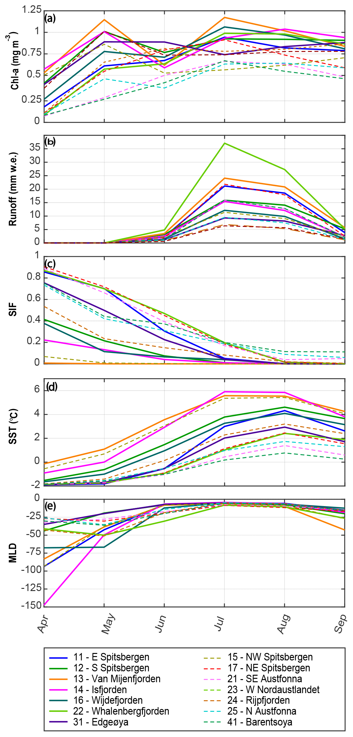
Figure 3 Average evolution of monthly variables for all primary hydrological regions and associated marine areas within 10 km distance from the coast: (a) chlorophyll a concentration, CHL; (b) specific glacier runoff, RUNOFF, per marine area; (c) sea-ice fraction, SIF; (d) sea-surface temperature, SST; and (e) mixed-layer depth, MLD. Solid lines represent regions that exhibit a significant positive correlation between RUNOFF and CHL (a), whereas dashed lines represent regions where no significant correlation was found.

In northeast Svalbard and Nordaustlandet (regions 17, 21–24), the 10-year monthly mean SIF is around 40 %–50 % in June and 20 % in July. Several regions in northern Svalbard showed a delayed association of CHL with SIF (regions 15, 16, 23; Fig. 2e) that indicates a delayed spring bloom. In this case, two separate production phases cannot be distinguished, at least at monthly temporal resolution. Instead, CHL during spring is low and steadily increases towards a maximum in July (e.g., regions 17, 21, 25). MLD during springtime (April) varies from up to 150 m in western Spitsbergen to around 30 m in northeast Svalbard and typically shallows in late spring to early summer (May–June). The shallowing MLD coincides with rising SST, suggesting that solar heating plays an important role in initiating stratification. Stable stratification of surface waters, as indicated by a shallow MLD, is already established when significant glacier runoff starts in July. Generally lower CHL in June than May suggests that phytoplankton may be nutrient limited when glacial melting sets in. The peak meltwater discharge coincides with elevated CHL during summer (July–August). Glacier runoff terminates in September, which may lead to the observed increase in the MLD, along with the recession of solar insulation and, possibly, initiation of wind-induced autumn mixing. Vertical mixing, as evident in a deepening of the MLD, may supply the photic zone with limiting nutrients, which could explain sustained CHL well into autumn, as observed in a northeast Greenland fjord (Holding et al., 2019).

5.4 Challenges and uncertainties of satellite-based surface chlorophyll a products

Although remotely sensed chlorophyll a is a commonly used proxy of phytoplankton biomass, there are several limitations to this approach. Firstly, data sampling relies on sufficient daylight, clear skies and largely sea-ice free conditions as ocean color sensors cannot detect ice algae or phytoplankton cells beneath sea ice (Arrigo, 2014). For Svalbard, chlorophyll a observations are typically limited to late March to early September. In the beginning and end of the acquisition period, spatial sampling is generally poor due to the persistence of sea ice and limited daylight (low sun angles). Spatial sampling is also poor under cloudy conditions, typical for Svalbard during summertime. The variable sampling intensity was accounted for in the statistical analysis as 8 d periods and regions with many satellite observations of CHL were given more weight in the analysis than periods and regions with few observations. Secondly, although the algorithm used to estimate CHL from surface reflectance accounts for the possible presence of inorganic particles, bias from inorganic particles originating from glacial meltwater cannot be ruled out. Some fjords of Svalbard are heavily influenced by suspended sediments from terrestrial or subglacial runoff which influences ocean color significantly (e.g., Dowdeswell et al., 2015; How et al., 2017; McGovern et al., 2020). Thirdly, subsurface maxima of chlorophyll a, as may occur in summer situations, are easily missed by satellite sensors because data retrieval is restricted to the upper layer of the water column down to the 1 % photosynthetically available radiation (Lee et al., 2007). It should therefore be kept in mind that our results show what happens in near-surface layers and not the entire water column. Subsurface chlorophyll a maxima are common in the Arctic Ocean (Arrigo et al., 2011; Ardyna et al., 2013) and have also been reported for Svalbard (Hop et al., 2019). Furthermore, phytoplankton can rapidly respond to reduced light availability, for example due to suspended matter, by increasing the chlorophyll a concentrations in their cells (Finkel, 2001; Finkel et al., 2004). It is therefore uncertain whether possible increased chlorophyll a concentrations at high meltwater runoff also reflect increased phytoplankton biomass. Further verification of remotely sensed chlorophyll a as a proxy of phytoplankton biomass in complex Arctic waters is required to gain more confidence in the results from our statistical analysis. This can only be achieved by in situ observations, extensive in both space and time, including simultaneous measurements of phytoplankton biomass, glacier runoff and nutrient concentrations in different water masses.

6 Conclusions

We investigated the effect of glacier runoff on regional-scale phytoplankton dynamics in Svalbard by combining chlorophyll a from satellite ocean color with glacier mass-balance modeling. Statistical analysis of regional time series revealed significant positive associations of CHL and RUNOFF for 7 out of 14 primary hydrological regions. The association of regional-scale CHL with RUNOFF is typically restricted to the major fjord systems and within 10 km distance from the coast. For regions characterized by open coastal conditions and beyond 10 km distance from the coast, the relationship between glacier runoff and marine primary production generally vanishes. Our results suggest that the overall effect of glacier runoff on marine primary production in these regions is positive despite counteracting effects of glacier runoff on the availability of light and essential nutrients, both of which are required for an increase in phytoplankton biomass.

We find that regions that display significant positive associations between CHL and RUNOFF have a 26 % higher mean summertime chlorophyll a and a 19 % higher mean annual maximum chlorophyll a compared to regions without such associations. Our analysis suggests that an increase in specific runoff of 10 $\mathrm{mm}\mathrm{w}.\mathrm{e}.\mathrm{8}{\mathrm{d}}^{-\mathrm{1}}$ raises regional summertime chlorophyll a concentrations by 5.2 % to 20.0 %, or 9.3 % on average, with a standard deviation of 4.6 %. During the annual peak discharge the effect is even larger, when glacier runoff is associated with 13.1 % to 50.2 % increase in chlorophyll a or 28.4±13.5 % on average. Glacier runoff thus facilitates a secondary phytoplankton bloom in July to August, typically following a spring bloom in May and a minimum in June, in line with in situ observations from Greenland (e.g., Juul-Pedersen et al., 2015). In terms of monthly mean CHL, the magnitude of the summer bloom is similar or may even exceed that of the spring bloom.

A common characteristic of regions which display significant positive associations between CHL and RUNOFF, i.e., the major fjord systems in Svalbard, is that they receive high volumes of glacier runoff per marine area. Mean specific runoff rates and specific mean annual peak runoff rates exceed those in open coastal regions by 46 % and 69 %, respectively. The primary hydrological regions associated with the fjord systems are also characterized by a highly variable glacier coverage, ranging from 35.5 % to 81.2 %, as well as glacier area drained through tidewater glaciers, ranging from 40.2 % to 87.4 %. This indicates that upwelling effects of nutrients from subglacial discharge plumes at a few tidewater glaciers may be sufficient to fuel regional-scale primary production. Alternatively, other mechanisms, such as enhanced estuarine circulation, driven by runoff from both land- and marine-terminating glaciers and down-fjord winds, may play a role.

To our knowledge, this study is the first to link large-scale chlorophyll a from satellite ocean color, an indicator of phytoplankton biomass, with glacier runoff from glacier mass balance modeling. Statistical analysis allowed us to identify and quantify significant associations between glacier runoff and regional chlorophyll a. We empirically show that glacier-runoff effects on primary production in Svalbard are mainly restricted to the major fjord systems and do not extend far outside the mouth of the fjords and onto the shelves. As we also consider physical-ocean and sea-ice variables in our statistical analysis, we are able to identify other environmental factors controlling regional summertime chlorophyll a dynamics in Svalbard. These factors include sea-ice conditions, especially in northern Svalbard, pointing at the influence of persistent sea ice and late sea-ice breakup. Furthermore, associations of CHL with SST and MLD along the West Spitsbergen Shelf indicate the role of the West Spitsbergen Current, i.e., the advection of warm saline and nutrient-rich water masses of Atlantic origin. Our method can be applied on a regional to pan-Arctic scale, thereby complementing valuable in situ observations which are only available from a few sites and often of short duration, thus not capturing inter-seasonal to interannual variability.

Appendix A: Partial effects of environmental variables on chlorophyll a

Figure A1 Partial effects of environmental variables on chlorophyll a, CHL, within 10 km from the coast. Each row shows the model (Eq. 1) for one hydrological region (Table 1). Each panel shows the relationship between a predictor variable (x axes) and CHL (y axes), with lines showing estimated partial effects and points showing partial residuals. Blank panels imply that the variable was not selected. Asterisks show statistical significance at levels 5 % (^∗), 1 % (${}^{\ast \ast }$) or 0.1 % (${}^{\ast \ast \ast }$).

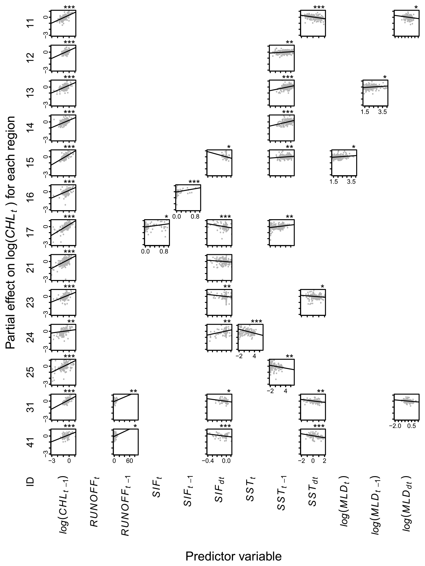
Figure A2 Partial effects of environmental variables on chlorophyll a, CHL, within 10 to 20 km from the coast. Each row shows the model (Eq. 1) for one hydrological region (Table 1). Each panel shows the relationship between a predictor variable (x axes) and CHL (y axes), with lines showing estimated partial effects and points showing partial residuals. Blank panels imply that the variable was not selected. Asterisks show statistical significance at levels 5 % (^∗), 1 % (${}^{\ast \ast }$) or 0.1 % (${}^{\ast \ast \ast }$).

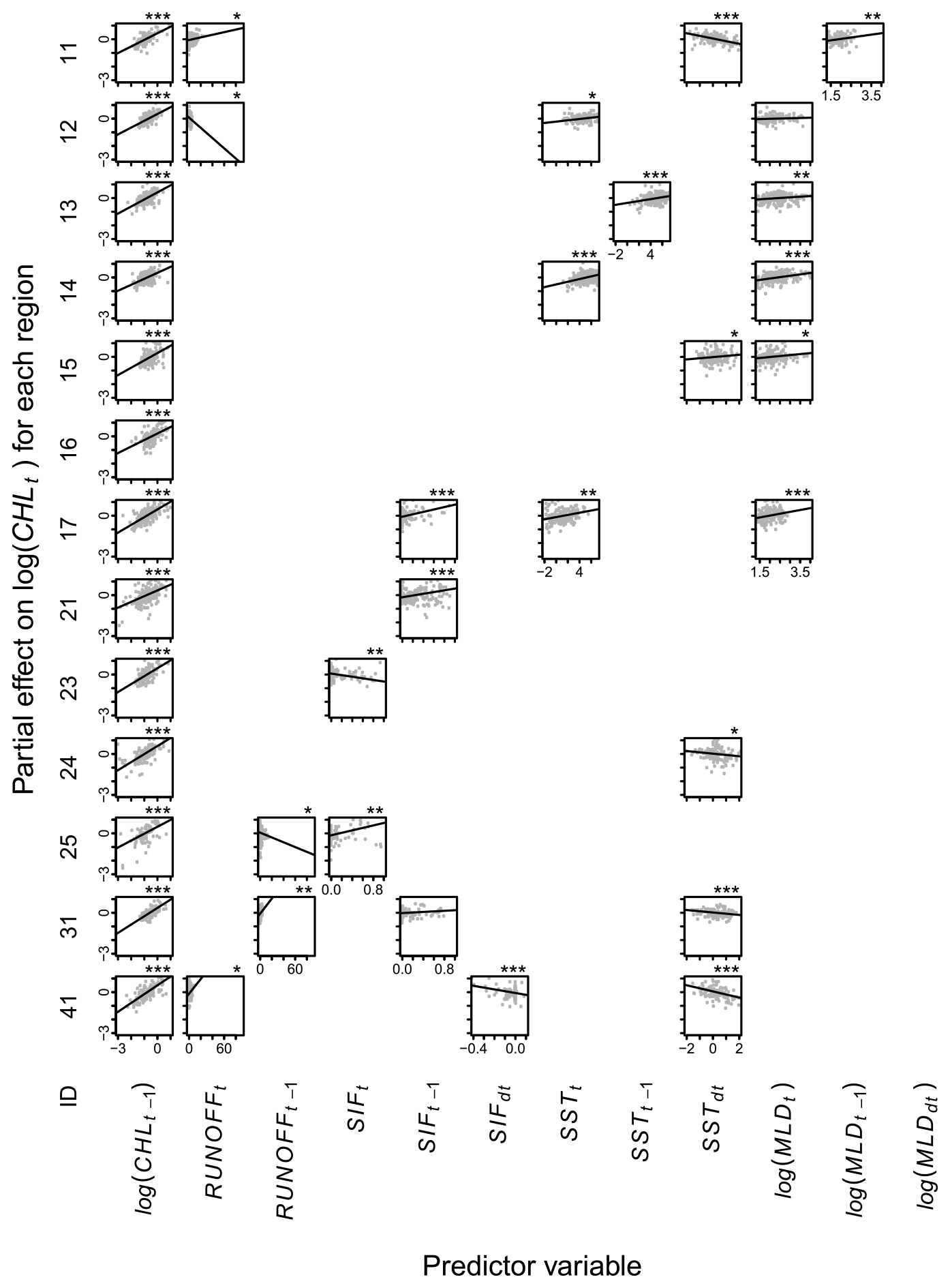
Figure A3 Partial effects of environmental variables on chlorophyll a, CHL, within 20 to 50 km from the coast. Each row shows the model (Eq. 1) for one hydrological region (Table 1). Each panel shows the relationship between a predictor variable (x axes) and CHL (y axes), with lines showing estimated partial effects and points showing partial residuals. Blank panels imply that the variable was not selected. Asterisks show statistical significance at levels 5 % (^∗), 1 % (${}^{\ast \ast }$) or 0.1 % (${}^{\ast \ast \ast }$).

Table A1 Summary of models for regions within 0 to 10 km from the coast. The model equations give parameter estimates with standard errors and statistical significance in brackets (${}^{\ast }P<\mathrm{0.05};{}^{\ast \ast }P<\mathrm{0.01};{}^{\ast \ast \ast }P<\mathrm{0.001}$). N is the sample size, and R² is the proportion of variance explained. ΔAIC₀ is the difference in the Akaike information criterion corrected for small sample size between the selected model and a null model with CHL in the previous time step, log (CHL_t−1), as the only predictor. ΔAIC_E is the difference in the Akaike information criterion corrected for small sample size between the selected model and an environmental model with RUNOFF excluded from the predictor variables.

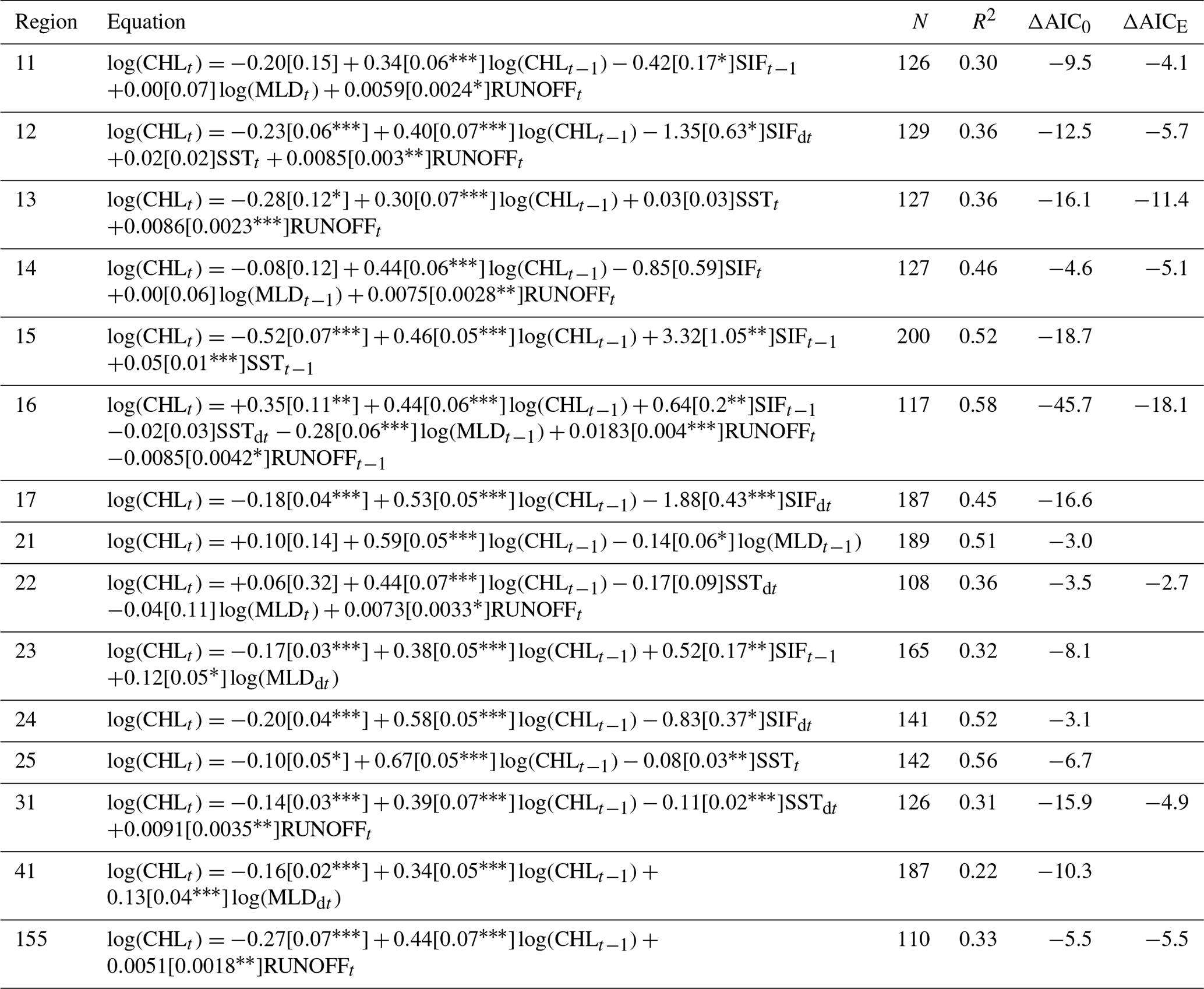
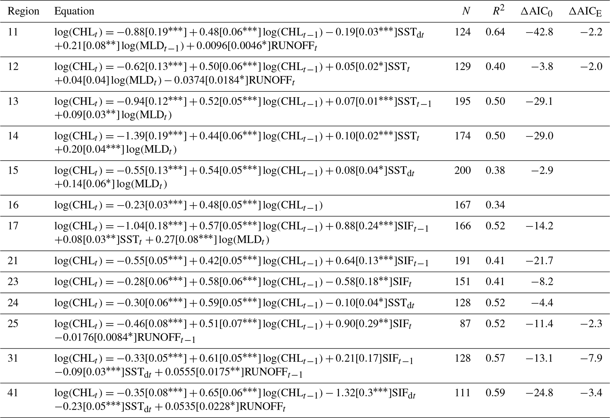
Table A2 Summary of models for regions within 10 to 20 km from the coast. The model equations give parameter estimates with standard errors and statistical significance in brackets (${}^{\ast }P<\mathrm{0.05};{}^{\ast \ast }P<\mathrm{0.01};{}^{\ast \ast \ast }P<\mathrm{0.001}$). N is the sample size, and R² is the proportion of variance explained. ΔAIC₀ is the difference in the Akaike information criterion corrected for small sample size between the selected model and a null model with CHL in the previous time step, log (CHL_t−1), as the only predictor. ΔAIC_E is the difference in the Akaike information criterion corrected for small sample size between the selected model and an environmental model with RUNOFF excluded from the predictor variables.

Table A3 Summary of models for regions within 20 to 50 km from the coast. The model equations give parameter estimates with standard errors and statistical significance in brackets (${}^{\ast }P<\mathrm{0.05};{}^{\ast \ast }P<\mathrm{0.01};{}^{\ast \ast \ast }P<\mathrm{0.001}$). N is the sample size, and R² is the proportion of variance explained. ΔAIC₀ is the difference in the Akaike information criterion corrected for small sample size between the selected model and a null model with CHL in the previous time step, log (CHL_t−1), as the only predictor. ΔAIC_E is the difference in the Akaike information criterion corrected for small sample size between the selected model and an environmental model with RUNOFF excluded from the predictor variables.