Modeling interactions between tides, storm surges, and river discharges in the Kapuas River delta

The Kapuas River delta is a unique estuary system on the western coast of the island of Borneo, Indonesia. Its hydrodynamics are driven by an interplay between storm surges, tides, and river discharges. These interactions are likely to be exacerbated by global warming, leading to more frequent compound flooding in the area. The mechanisms driving compound flooding events in the Kapuas River delta remain, however, poorly known. Here we attempt to fill this gap by assessing the interactions between river discharges, tides, and storm surges and how they can drive a compound inundation over the riverbanks, particularly within Pontianak, the main city along the Kapuas River. We simulated these interactions using the multi-scale hydrodynamic model SLIM (Second-generation Louvain-la-Neuve Ice-ocean Model). Our model correctly reproduces the Kapuas River's hydrodynamics and its interactions with tides and storm surge from the Karimata Strait. We considered several extreme-scenario test cases to evaluate the impact of tide–storm–discharge interactions on the maximum water level profile from the river mouth to the upstream part of the river. Based on the maximum water level profiles, we divide the Kapuas River's stream into three zones, i.e., the tidally dominated region (from the river mouth to about 30 km upstream), the transition region (from about 30 km to about 150 km upstream), and the river-dominated region (beyond 150 km upstream). Thus, the local water management can define proper mitigation for handling compound flooding hazards along the riverbanks by using this zoning category. The model also successfully reproduced a compound flooding event in Pontianak, which occurred on 29 December 2018. For this event, the wind-generated surge appeared to be the dominant trigger.

1 Introduction

Global warming leads to more frequent tropical storms, rising sea levels, and more intense rainfalls, which all concur in increasing the occurrence of compound flooding events in a coastal area and its surrounding environment (Bevacqua et al., 2020). Such disasters impact the lives of more and more people worldwide (Moftakhari et al., 2015). Compound flooding occurs when dry low-lying land (over a coastal area) is flooded by water from the ocean and the river. Compound flooding is driven by the interaction between a coastal inundation and a riverine inundation. The former happens from the seaward direction due to high (spring) tides and storm surges, while the latter occurs from the landward due to high discharges from upstream rivers. Coastal communities, which have been growing in population over the past decades, have become increasingly vulnerable to those events. Cities located along an estuary are at the crossroad between the ocean and the river catchment, hence particularly vulnerable (Herdman et al., 2018; Vitousek et al., 2017; Zhang and Liu, 2017).

One of the most significant drivers that can trigger compound flooding over a coastal area is storm surges (Herdman et al., 2018; Zijl et al., 2013). A storm surge is defined as the difference between the observed water level and the expected water level that results from tidal dynamics in a coastal area. A storm surge effect on usual tidal dynamics is the altered timing of high and low water through non-linear processes (Zijl et al., 2013). A storm surge is composed of low- and high-frequency components (Spicer et al., 2019). The former modifies the non-tidal water level, and the latter represents a tide–surge interaction during the event. A storm surge is generally quantified by the skew surge (Giloy et al., 2019), which is a tidal cycle average measurement – the difference between the observed height and the expected height. It reflects the level of surge generated over a tidal cycle. To mitigate compound flooding hazards in a coastal area, a storm surge is a critical component that should always be taken into account.

Several factors must be considered regarding the assessment of compound flooding risks in a river delta. The first factor is the coincidence of the sources (Herdman et al., 2018), which means there is a possibility for the delta to receive an extreme flow from the upstream, while, at the same time, there could be an intense surge occurring in the tide or excessive rainfall over the coastal area. The second factor is the dependency and interdependency of the sources, indicating whether the interaction between these sources (extreme flows, tides, and excessive rainfall) could significantly impact the inundation processes (Bilskie and Hagen, 2018; Herdman et al., 2018; Santiago-Collazo et al., 2019). Other important factors include the vegetation properties along the riverbanks that resist the flow of water, the vegetative properties over the estuary that reduce the momentum transfer of wind, the landscape characteristics of the coastal area, and how they interacted with each other (Twilley et al., 2016).

Flooding events in a delta area can be simulated and assessed using hydrodynamic models (Deb and Ferreira, 2017; Olbert et al., 2017; Patel et al., 2017). The most useful models are those that can seamlessly simulate the processes occurring along the land–sea continuum, which corresponds to the area encompassing the coast, the estuary, and the river channels. Such models allow for a study of past flooding events and an assessment of flood mitigation strategies (Vu and Ranzi, 2017). However, realistic input variables and forcing are needed to create an accurate physics-based hydrodynamic model. Since the processes that drive compound flooding are three-dimensional, a 3D model is the most appropriate tool to evaluate the event. However, the area of interest represents a well-mixed and relatively shallow waterbody. Therefore, we applied a 2D barotropic solution to reduce computational costs (Huybrechts et al., 2010; Néelz, 2009).

As an archipelago country with about 100 000 km of coastlines, Indonesia is faced with significant coastal flooding risks (World Meteorological Organization, 2019). Indonesian coastal flood hazards are classified as high (GFDRR, 2022). It means that the potentially damaging waves are expected to flood the coasts at least once every 10 years. Based on this risk and concerns about the impact of climate change in the future, a hazard assessment study in Indonesian low-lying coastal areas (such as deltas) has become critical for Indonesian water management authorities. One area in Indonesia that is vulnerable to coastal or even compound flooding is the Kapuas River delta. In this delta, flooding events happen more than once a year (Wells et al., 2016). Unfortunately, there is no previous study addressing the process that underlies the flood events in there. The previous study (Hidayat et al., 2014) successfully evaluated the inundation frequency, but it only did so for the upstream area and did not evaluate the underlying process. Therefore, this study attempts to fill in the gap and provide the first compound flood assessment in the area.

This paper investigates the interaction between tides, storm surges, and river discharges in the Kapuas River downstream and its surrounding area. We use a 2D hydrodynamic model to simulate the interaction between these driving forces and their effects on the compound flooding in the Kapuas River delta, particularly in Pontianak. Then, we create a detailed flood assessment, determine the area's extent, and calculate the inundation depth. As a case study, we implemented the model explicitly to a compound flooding event on 29 December 2018.

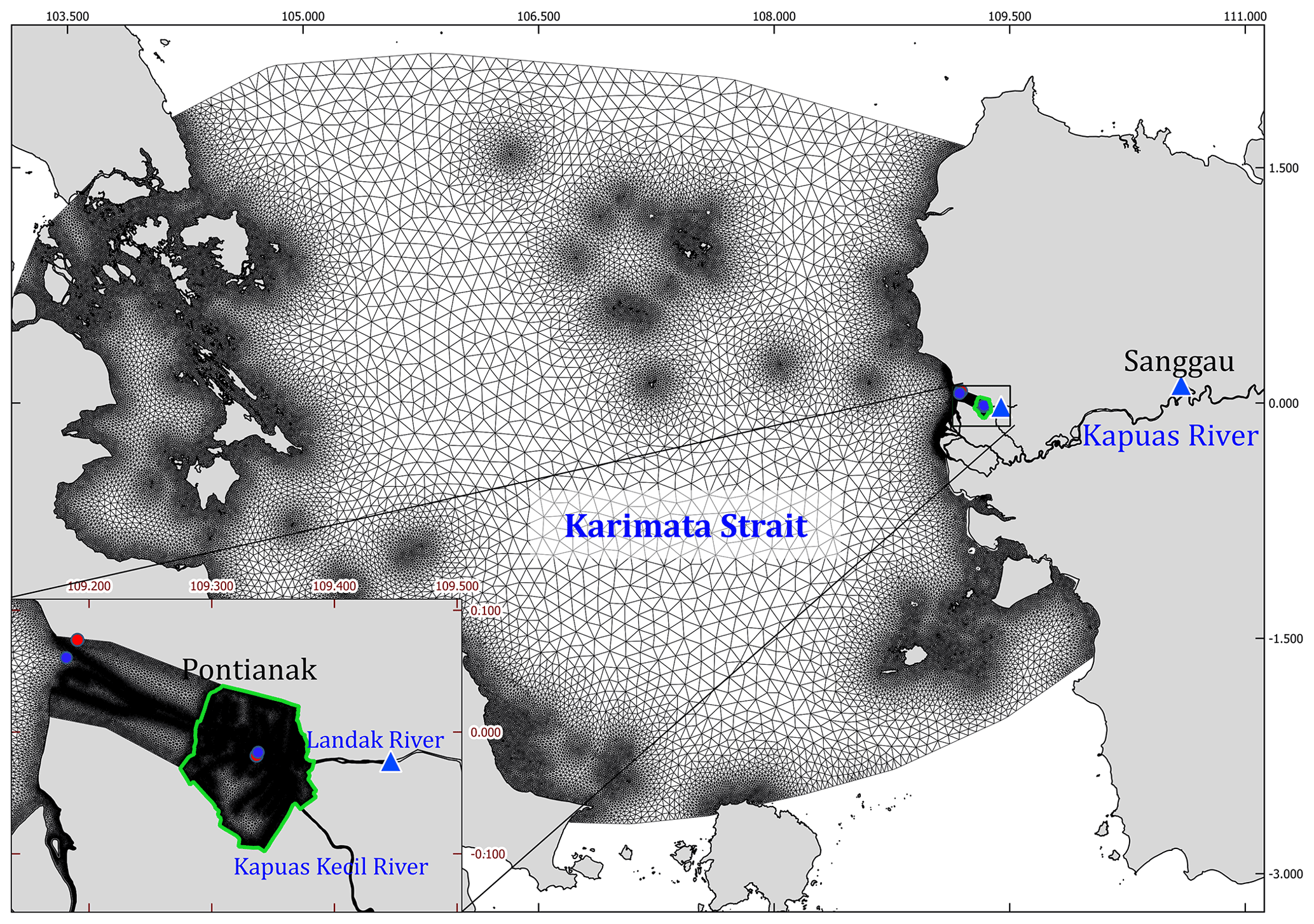
Figure 1 The region of interest includes the Karimata Strait, the Kapuas River and its estuary, and the city of Pontianak, whose limits are shown in green. The unstructured mesh is made of triangles whose resolution ranges from 50 m over the river and estuary to 1 km near the coastlines and 10 km in the middle of the Karimata Strait. The mesh is composed of 206 359 triangular elements. Red dots represent the weather station's locations, and blue dots represent the tidal validation points (on the left is the river mouth; on the right is the Pontianak Maritime Meteorological Station observation point, where the weather and the tidal validations points are superimposed). Blue triangles depict the river boundary where discharges are imposed in the model. The background map was retrieved from OpenStreetMap (https://planet.osm.org, OpenStreetMap contributors, 2021). © OpenStreetMap contributors 2017. Distributed under the Open Data Commons Open Database License (ODbL) v1.0.

2 Materials and methods

2.1 Area of interest

The Kapuas River flows from the center of the island of Borneo (Indonesia) toward the Karimata Strait on the western coast (Fig. 1). The river is one of the longest island rivers in the world, with a length of about 1143 km (Goltenboth et al., 2006). The Kapuas River basin is located on the Equator with high air temperature and humidity throughout the year. The river basin spreads over about 8.28 × 10⁴ km², with about 66.7 % of it consisting of forests (Wahyu et al., 2010). The topography of the river comprises hills over its upstream and plains over its downstream. The river flows into the Karimata Strait through five major branches (MacKinnon et al., 1996).

The Kapuas Kecil is the second largest distributary of the Kapuas. The river branch starts from a Kapuas branch in the district of Rasau Jaya and ends at the estuary area in the district of Jungkat. In the middle of its streamflow (about 20 km before the river mouth), the Landak tributary joins the Kapuas Kecil. The junction is located in the city of Pontianak, the capital of the province of West Kalimantan, Indonesia, placing the urban area at the highest risk of flooding among other areas along the Kapuas riverbanks.

Pontianak is the most populated urban area on the western coast of the island of Borneo, with a population of about 600 000 people that keeps increasing. The city is located on low-lying land and has 61 canals spread across the area. Most of these canals flow in the Kapuas Kecil River (Pemerintah Kota Pontianak, 2021). As a consequence of its geographical situation, the city often experiences inundations.

2.2 Hydrodynamic model

The interplay between the river discharges, the tides, and wind surges from the sea and their effect on the inundation processes in Pontianak is investigated by using the Second-generation Louvain-la-Neuve Ice-ocean Model (SLIM, https://www.slim-ocean.be/, last access: 3 April 2021). The model equations are discretized with the discontinuous Galerkin finite element method. The model uses an unstructured mesh whose resolution can vary in space. The model has successfully been applied to several areas, such as the Great Barrier Reef (Lambrechts et al., 2010), the Mahakam delta (Pham Van et al., 2016), the Scheldt estuary (Gourgue et al., 2013), and the Columbia River (Vallaeys et al., 2018).

Here, we use the wetting–drying barotropic version of SLIM that solves the conservative form of the shallow-water equations (SWEs):

$$\begin{array}{}\text{(1)}& {\displaystyle \frac{\partial H}{\partial t}}+\mathrm{\nabla }\cdot U=\mathrm{0},\text{(2)}& {\displaystyle }\begin{array}{rl}& {\displaystyle \frac{\partial U}{\partial t}}+\mathrm{\nabla }\cdot \left({\displaystyle \frac{UU}{H}}\right)+f{e}_z\times U-\mathrm{\nabla }\cdot \left(\mathit{\upsilon }\mathrm{\nabla }U\right)\\ & =\mathit{\alpha }gH\mathrm{\nabla }(H-h)-{\displaystyle \frac{\text{Cd}}{H^{\mathrm{2}}}}\mathrm{|}U\mathrm{|}U+{\displaystyle \frac{\mathrm{1}}{\mathit{\rho }}}{\mathit{\tau }}_{\text{wind}}-{\displaystyle \frac{H}{\mathit{\rho }}}\mathrm{\nabla }{p}_{\text{atm}},\end{array}\end{array}$$

where $U=H\stackrel{\mathrm{‾}}{u}$ is the horizontal transport, H is the water column height, h is the bathymetry, t is the time, and $\stackrel{\mathrm{‾}}{u}$ = (u,v) is the depth-averaged horizontal velocity and where α is a constant that is set to zero over dry elements and one over wet elements (Le et al., 2020), ∇ is the horizontal gradient operator, g = 9.81 m s⁻² is the gravitational acceleration, Cd is the bulk drag coefficient, f is the Coriolis parameter, e_z is the vertical unit vector pointing upward, υ is the horizontal eddy viscosity, ρ is the water density, τ_wind is the wind stress, and ∇p_atm is the atmospheric pressure gradient. Here, the wind stress (τ_wind) was computed with the Smith and Banke (1975) formula for the wind speed of less than 20 m s⁻¹ and was computed with the Moon et al. (2007) formula for wind speed higher than 20 m s⁻¹.

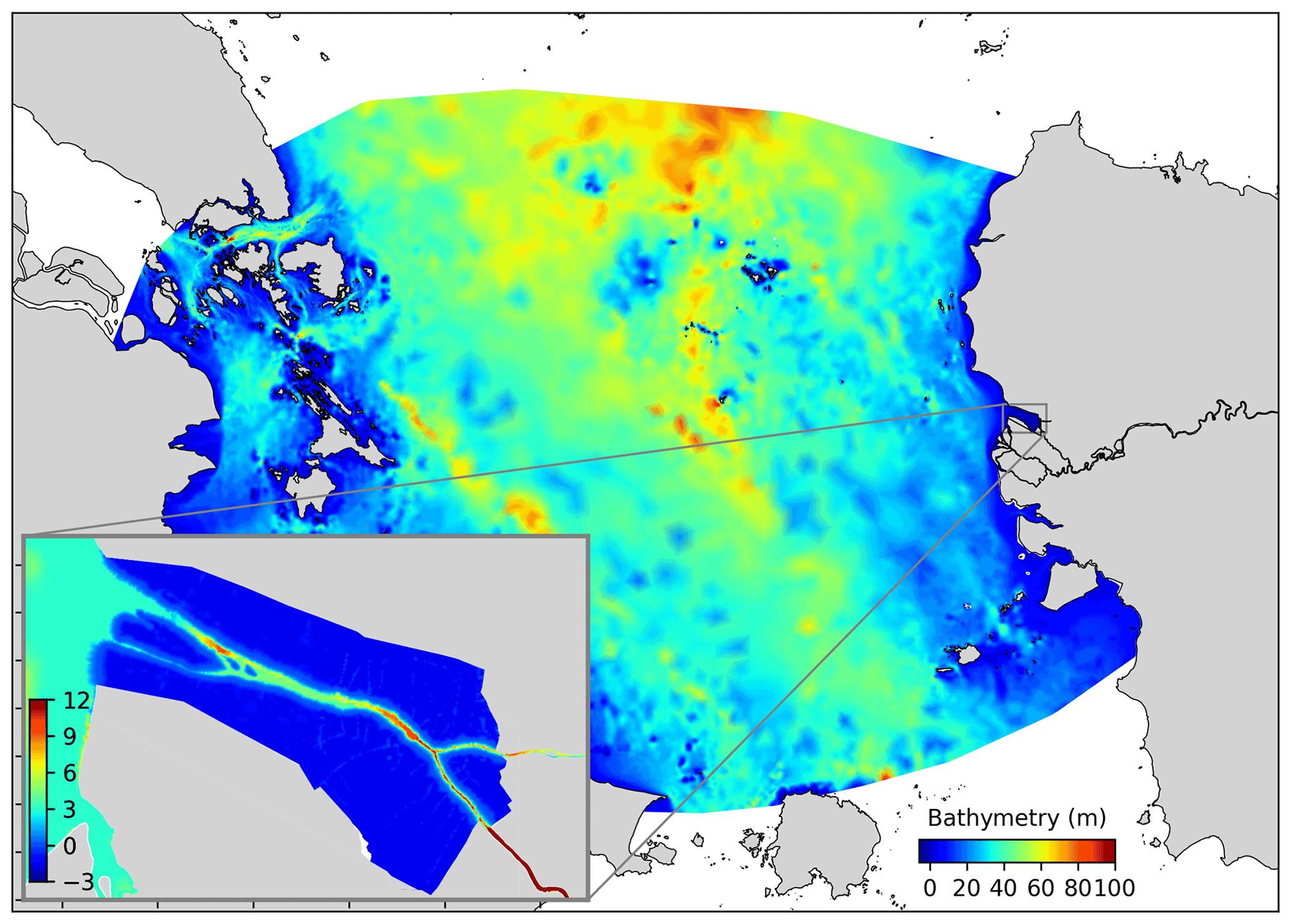
Figure 2 Bathymetry map, with positive values meaning under the mean sea level.

The model equations are solved using a wetting–drying algorithm with an implicit time-stepping scheme. With this algorithm, a mesh element can be defined as wet or dry. It requires a procedure that guarantees that the water column height (H) is always positive at the end of the time step to solve the equations. To achieve that, we set first a threshold h^∗ that indicates the water height below which an element is assumed to be dry (here h^∗ = 0.1 m). Then, we define a parameter representing the total water column height on an element as a combination of maximum water level and minimum bathymetry: s = $max\left(\mathit{\eta }\right)+min\left(h\right)$. When s is smaller than h^∗, gravity will be canceled on the element so that the artificial gradient of surface elevation would not remove water from an already-dry element (α=0). On the contrary, if s is greater than h^∗, then the gravitational force will be preserved as usual (α=1). The transition between α=0 and α=1 occurs smoothly. More details about this procedure can be found in Le et al. (2020).

2.3 Model setup

Before creating the model, we first define a domain covering both the ocean and the Kapuas River delta. Since we focused on evaluating the impact of tide–surge–discharge interaction on extreme water levels along the Kapuas Kecil branch (particularly in Pontianak), we leave out several distributaries that may not significantly influence that dynamics, such as the southern Kubu branch. Next, we mesh the domain, set the bathymetry and the bulk drag coefficient, define the boundary conditions (surface elevation and velocity), and finally impose some forcings. After the model is created and run successfully, we validate the results using observational data.

Here, we generate a multi-scale mesh of the entire domain by using the mesh-generation algorithm of Remacle and Lambrechts (2018). The mesh consists of 206 359 triangular elements. Fine mesh elements are used to accurately represent inundation events over the land area of Pontianak and along the Kapuas riverbanks, while the coarser mesh elements are used far away from the delta. The mesh resolution reaches 50 m along the Kapuas riverbanks and over the city of Pontianak. It decreases to 10 km in the middle of the Karimata Strait (Fig. 1).

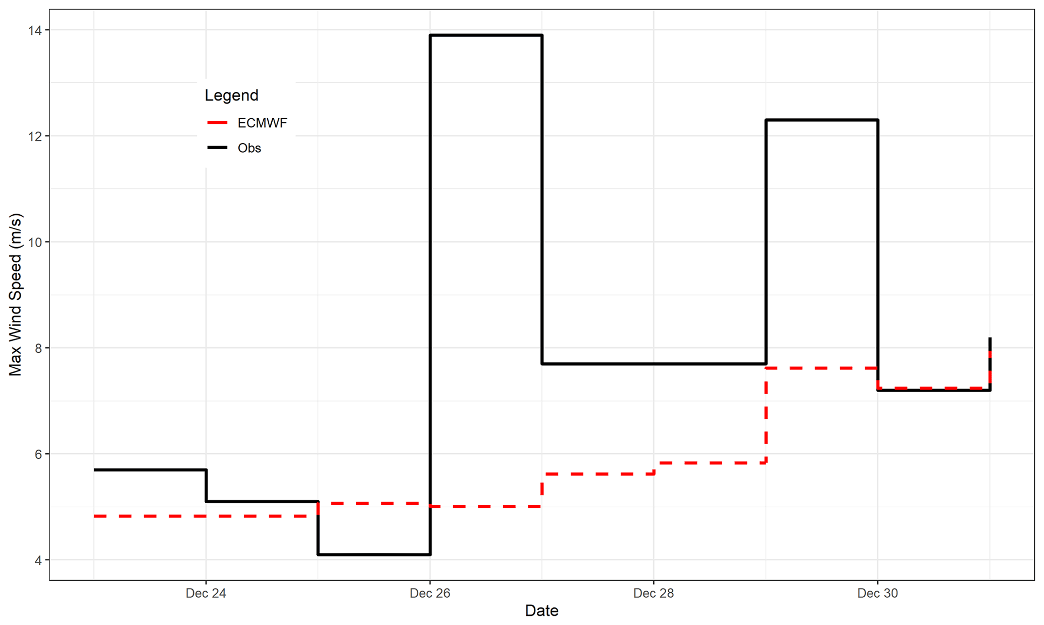
Figure 3 Maximum daily wind speed from ECMWF ERA5 compared to observations at the Kapuas Kecil River mouth. During strong wind events, the ERA5 data tend to underestimate the actual wind speed.

The bathymetry is created from a combination of three different data sources. The first is the river and estuary bathymetry obtained from the Indonesian Navy (Kästner et al., 2019) with a 100 m × 100 m grid resolution. The second is the Karimata Strait bathymetry, obtained from BATNAS (Badan Informasi Geospasial, 2018a) with a 180 m × 180 m grid resolution. The last is the digital elevation model from DEMNAS (Seamless Digital Elevation Model dan Batimetri Nasional; Badan Informasi Geospasial, 2018b) with 0.27 arcsec resolution. The Karimata Strait bathymetry shows that the strait is shallow (less than 100 m) and relatively flat (Fig. 2). On the other hand, the bathymetry of the river is more heterogeneous. The river is shallow in the estuary but deeper in the middle stream. The depth ranges from 1 m (in the estuary area) to 40 m in the middle stream area (Kästner et al., 2017). The Kapuas Kecil River, which flows through Pontianak, has a depth that decreases from 15 m in the middle stream to 1 m in the river mouth.

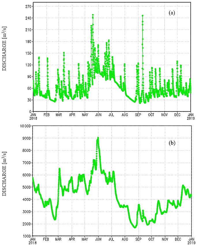
Figure 4 River discharge of (a) the Landak (prescribed at 0.0282^∘ S, 109.445^∘ E) and (b) the Kapuas (prescribed at 0.3623^∘ S, 109.6394^∘ E) retrieved from Wu et al. (2014).

The wind velocity and the atmospheric pressure data are the ERA5 reanalysis dataset obtained from the European Centre for Medium-Range Weather Forecasts (ECMWF). The data have a spatial resolution of 31 km (Hersbach et al., 2020), while the temporal resolution is hourly and available at 137 vertical levels (0 to 80 km from the surface). The model wind stress parametrization uses the wind speed at 10 m height. Unfortunately, compared with observational data from the Stasiun Klimatologi Mempawah (http://iklim.kalbar.bmkg.go.id, last access: 3 April 2021), measured at 10 m above the surface, there are clear differences in amplitude. The observed wind velocity is more significant than the wind velocity from ERA5 during a wind surge (Fig. 4). Therefore, in the case study, we adjust the magnitude of the wind input data (ERA5) during the wind surge event. We multiplied the wind magnitude with a ratio between both peaks (the observed and ERA5 data).

Next, we set the bulk drag coefficient to 2.5 × 10⁻³ over the ocean and 1.9 × 10⁻² (average bulk drag during December 2018, since it is slightly increasing with the river discharge) over the river part (Kästner et al., 2018). Both coefficients correspond to a sandy bed. Over the dry area, the drag coefficient is determined by two types of land cover (urban and non-urban area), as defined in the Copernicus Global Land Service land cover map (Buchhorn et al., 2020). For the urban area, the bottom drag coefficient is 2.05 (Hashimoto and Park, 2008). Over the non-urban area, it is set to 2.0, which corresponds to dense vegetation (Li and Busari, 2019).

Then, we imposed discharge at the rivers and tides at the open ocean for the open boundaries. Upstream of the rivers, we imposed the discharge of the Kapuas River and the Landak River. Since there are no observational data for both rivers, we set constant discharges for the simulations in some scenarios. However, to reconstruct the observed inundation (discussed in the case study), we imposed the discharges obtained from the Global Flood Monitoring System (GFMS). The GFMS estimated the global discharge based on Tropical Rainfall Measuring Mission (TRMM) Multi-satellite Precipitation Analysis and Global Precipitation Measurement data (Wu et al., 2014). The Kapuas River discharge is bigger than the Landak River discharge (Fig. 4). At the open boundaries in the ocean, we prescribed the tidal elevation and current of 15 harmonics from the global tide model dataset, the OSU (Oregon State University) TPXO (TOPEX/Poseidon) Tide Models TPXO9-atlas (Egbert and Erofeeva, 2002). We also prescribed global ocean circulation from HYCOM (HYbrid Coordinate Ocean Model; Chassignet et al., 2007) at these boundaries.

To evaluate the model performance, we performed the tidal analysis on the simulated surface elevation and compared it to the observed water level at the tide gauges. The analysis was conducted using the Unified Tidal Analysis and Prediction (UTide) Python package (Codiga, 2011). The tidal analysis assumes that a tidal signal is a linear combination of multiple sinusoidal signals associated with its astronomical forcing. Each of these signal components has a different phase, amplitude, and temporal frequency. The analysis aims to obtain tidal harmonic constituents. Since we only ran the model for a limited time duration (in order to minimize the computational cost), it is impossible to extract all tidal constituents from the model's signal output. As a rule of thumb to select the appropriate tidal constituent, we used the Rayleigh criterion (Godin, 2015). Based on this criterion, we obtained nine tidal constituents, i.e., K1, O1, Q1, P1, and J1 (as the representation of the diurnal components); M2 and S2 (as the representation of the semidiurnal components); and MK3 and MO3 (as the representation of the third-diurnal constituents).

To perform tidal analysis, water level signals were extracted and analyzed at two points. The first point is located at the river mouth (0.0617^∘ N, 109.1751^∘ E), and the second point (0.020431^∘ S, 109.33852^∘ E) is located along the Kapuas Kecil River within the city of Pontianak (Fig. 1). The second point is located about 20 km from the river mouth. At the first point, the model's output signal is compared with the tidal signal from the Indonesian Consortium of Oceanic and Atmospheric Prediction (ina-COAP) (Pusat Riset Kelautan, 2021). Meanwhile, for the second point, the model's signal output is compared to the observational data collected by the Pontianak Maritime Meteorological Station (PMMS).

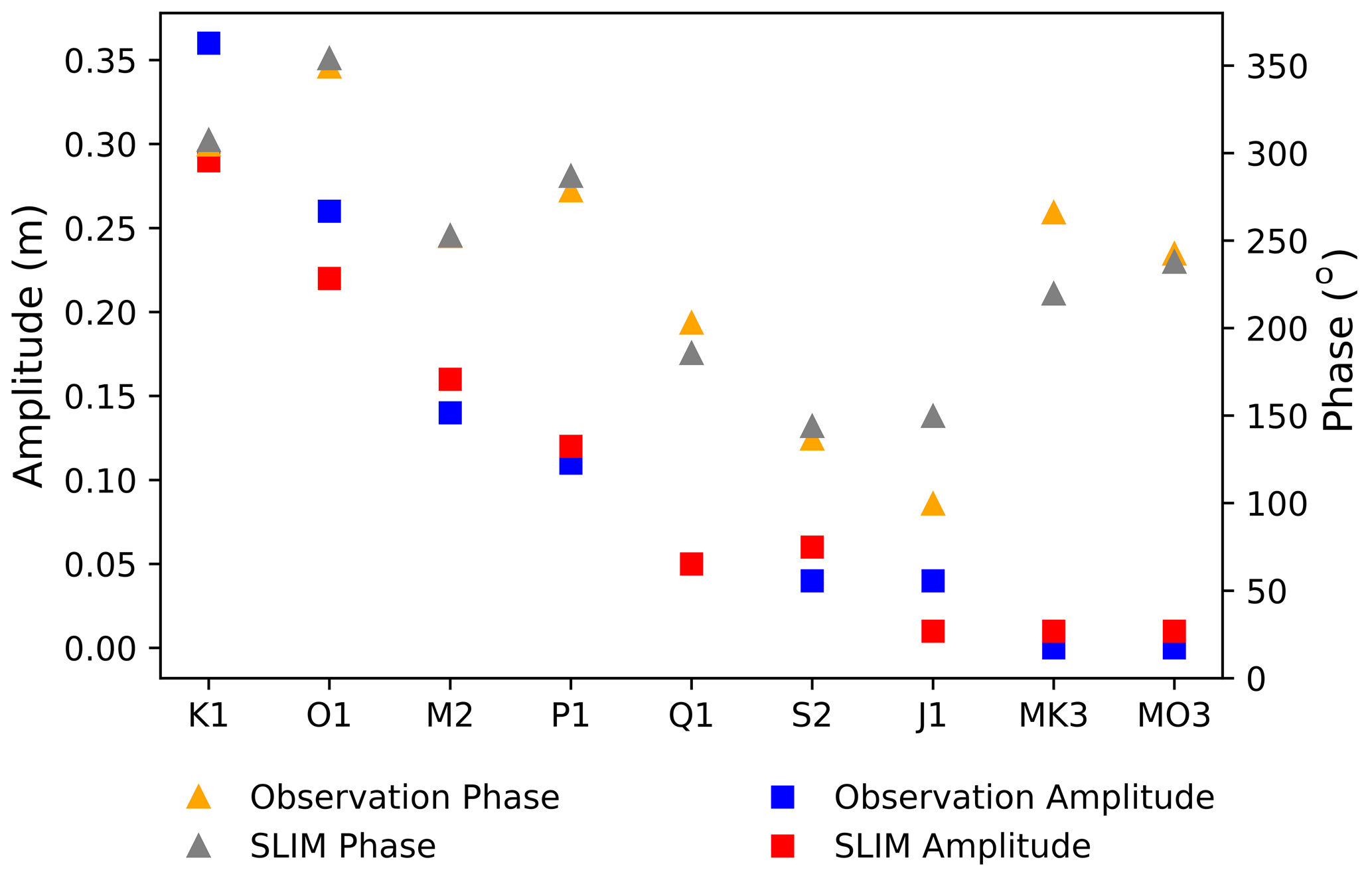
Figure 5 Observed and simulated tidal constituents (amplitude and phase) at the Kapuas Kecil River mouth (0.0617^∘ N, 109.1751^∘ E) during December 2018.

To quantify the agreement between the simulated water level and observation, we calculated the Nash–Sutcliffe efficiency (NSE) and root mean square error (RMSE) between both time series. The former coefficient measures how well the model's performance represents the observed data. NSE = 1 represents a perfect model; NSE = 0 depicts a model with a predictive skill the same as the mean of the observed data; and NSE < 0 informs that the mean of the observed data is a better predictor than the model output. The latter coefficient indicates the average of the difference in the peaks between both time series. Both of these coefficients were calculated using the library hydroGOF (goodness of fit) in R (Zambrano-Bigiarini, 2020).

In order to better investigate the inundation extent and depth over the city of Pontianak, we used the HEC-RAS model (Hydrologic Engineering Center River Analysis System; U.S. Army Corps of Engineers Hydrologic Engineering Center, 2022). We firstly created a second mesh to cover the computational domain over the city and used water levels from the SLIM output model as the boundary conditions (Fig. 12). The second mesh has a 10 m resolution; hence it can better represent canals that spread in the city. Like the SLIM model, the HEC-RAS model also solves the shallow-water equations (SWEs).

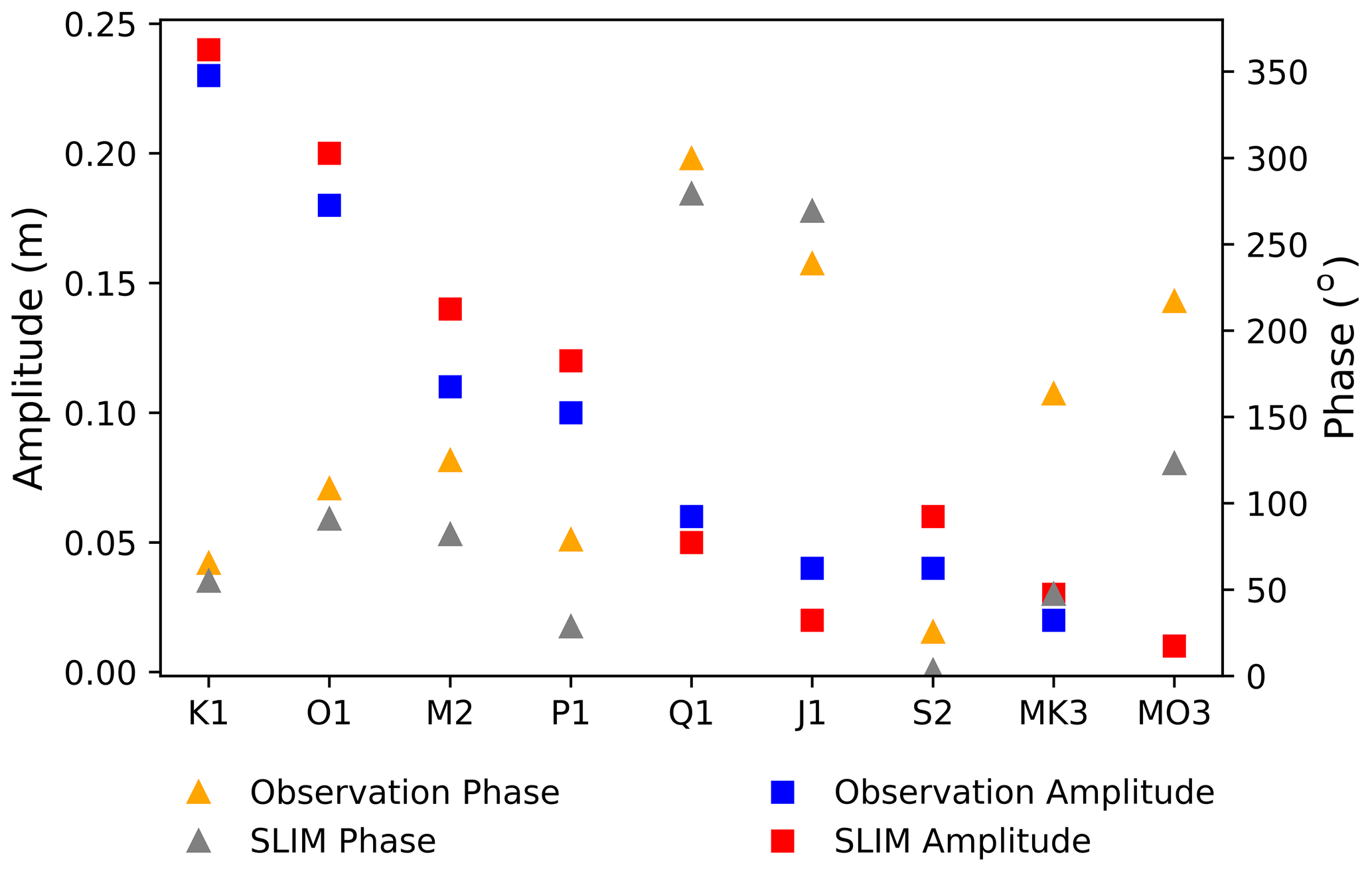
Figure 6 Observed and simulated tidal constituents (amplitude and phase) in the middle of Pontianak (0.020431^∘ S, 109.33852^∘ E) during December 2018.

3 Results

3.1 Model validation

The validation results show a good agreement between the model output and the ina-COAP's tidal signal at the Kapuas Kecil River mouth (0.0617^∘ N, 109.1751^∘ E), with a coefficient of determination of R² = 0.95 and RMSE = 0.09 m. At this point, the model produces a tidal signal that has constituent attributes (phase and amplitude) similar to the ina-COAP's tidal signal. The diurnal components explain about 90.69 % of the total variances of the estuary's tidal dynamics, while the semidiurnal components only account for about 9.31 % (see Fig. 5 and Appendix Table A1 for more detail). Next, the tidal analysis result at the observation point in Pontianak (0.020431^∘ S, 109.33852^∘ E) also shows a good agreement between the model output and observation with a coefficient of determination of R² =  0.83 and RMSE = 0.14 m. The model output signal also has similar constituents attributed to the PMMS observational water level signal (Fig. 6 and Appendix Table A2). At this point, the diurnal components explain about 89.6 % of the total variances of the estuary's tidal dynamics, which is lower from the river mouth. Then, the semidiurnal components account for about 9.9 %, and the shallow-water terdiurnal components explain the rest. The analysis at this second point also confirms that the model successfully reproduces the observed hydrodynamics.

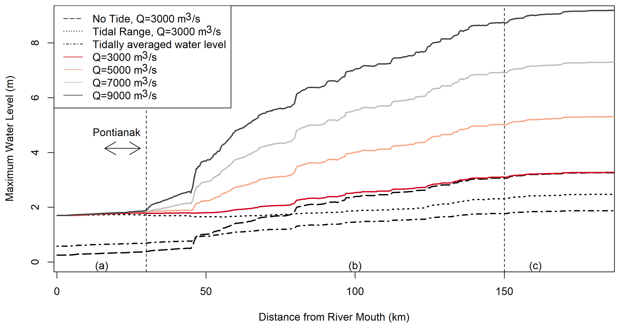
Figure 7 River discharge affecting the maximum water level, with measurements for the (a) tidally dominated region, (b) transition region, and (c) river-dominated region. The dashed vertical lines indicate the limits between the different regions. The arrow shows the river stream that flows inside Pontianak, where the population is the densest in the domain.

3.2 The impact of river discharges on the river's maximum water level

The impact of the Kapuas River upstream discharge on its downstream hydrodynamics is assessed by imposing different discharge values, ranging from 3000 to 9000 m³ s⁻¹ (the highest discharge based on the simulated data in 2018; see Fig. 4 and Table A3). Only 17 % of these values will divert to the Kapuas Kecil branch, while 83 % of it continues to flow through the Kapuas Besar (Kästner and Hoitink, 2019). Meanwhile, the Landak River upstream discharge is set to 300 m³ s⁻¹ in all scenarios. The tides used in the ocean part were retrieved from TPXO for December 2018, with a tidal range of 1.8 m at the river mouth. The maximum water level (MXWL) at different points along the Kapuas River stream is then calculated based on these different discharge scenarios (Fig. 7). The MXWL profiles show that the river discharge dominates the maximum water level from the river upstream to about 150 km before the river mouth. The MXWL profile increases along with the discharge's increases, so the water level fluctuation in this stream part can be said to be river-dominated. Within about 150 km from the river mouth, the MXWL profiles between the “with-tides” and “without-tides” scenarios show a different pattern. The MXWL profiles no longer increase along with the upstream discharge's increases. In fact, the closer to the river mouth, the lower the gap between the MXWL profiles. Then, all MXWL profiles converge at about 30 km before the river mouth. We define the part of the river as a transition region. Meanwhile, at about 30 km from the river mouth, the discharge variations have almost no influence on the MXWL. In this area, the tides control the MXWL, so we define this river part as a tidally dominated region.

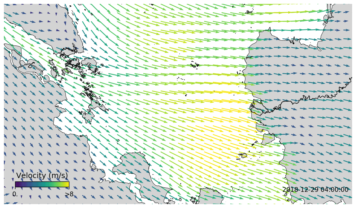
Figure 8 Wind direction and magnitude over the domain on 29 December 2018 at 04:00 UTC.

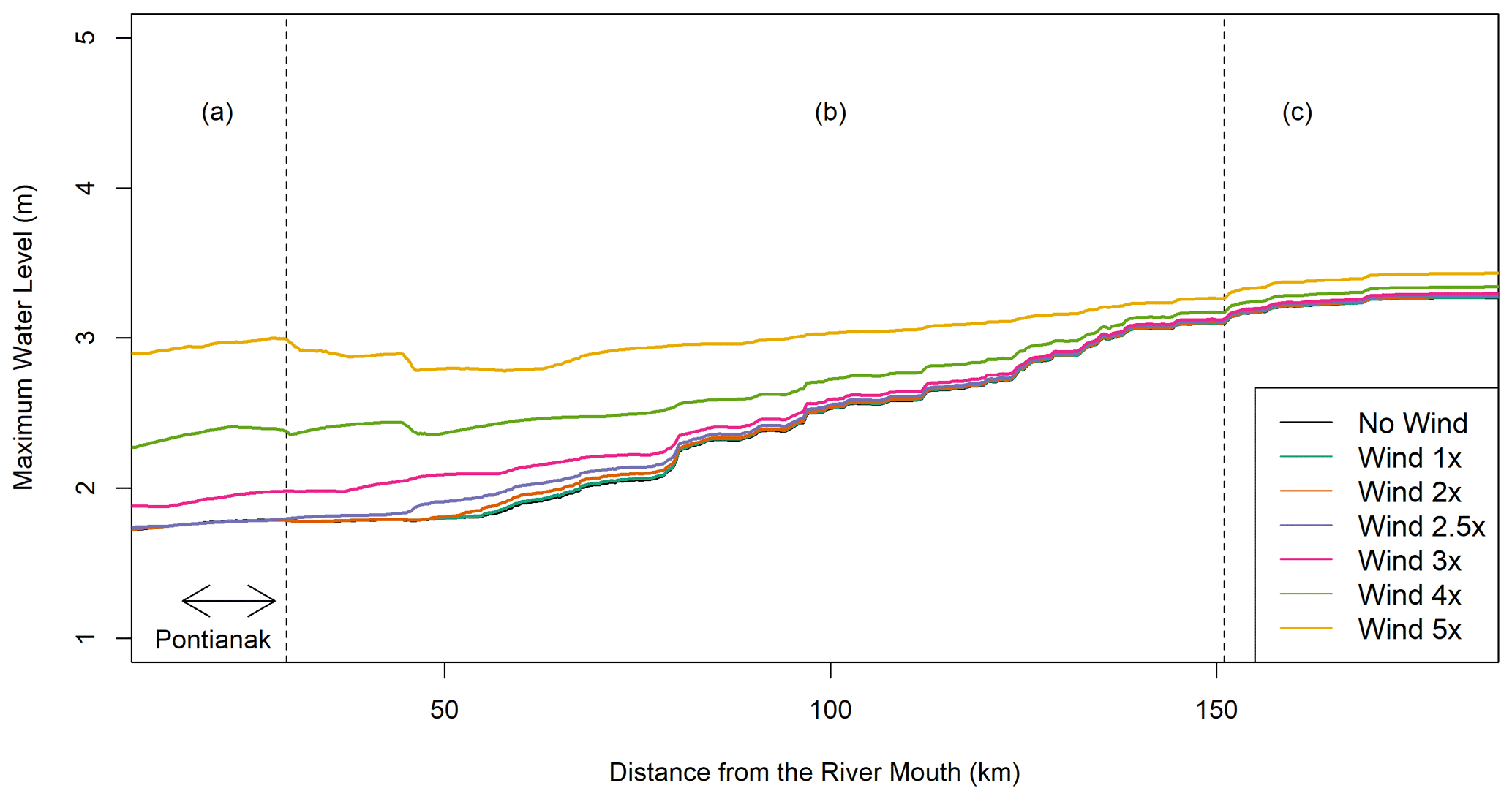
Figure 9 Wind surge affecting the maximum water level, with measurements for the (a) tidally dominated region, (b) transition region, and (c) river-dominated region. The arrow shows the river stream that flows inside Pontianak.

3.3 The impact of wind surges on the river's maximum water level

To evaluate the storm surge effect, we consider wind velocity scenarios (Fig. 8). For each scenario, we multiplied the wind speed over the domain during the inundation event by a constant value ranging from 1 to 5 (Table A3). Then, we evaluated their impact on the MXWL profiles along the Kapuas Kecil River stream. Based on the profiles (Fig. 9), we thus know that the increasing wind speed beyond 16 m s⁻¹ (the highest wind speed in scenario Wind_2x) changes the MXWL distribution profile. The stronger the wind speed, the higher the MXWL. On the contrary, if the wind speed is less than 16 m s⁻¹, the MXWL profiles remain the same.

Figure 10 Wind surge duration affecting the increasing water level in Pontianak. Please note that the date format used in this figure and below is year-month-day.

Furthermore, the storm surge strongly dominates the MXWL from the river mouth to about 30 km up the river. If the wind speed exceeds 20 m s⁻¹ (the highest wind speed in scenario Wind_2.5x), the MXWL profile will increase linearly due to the wind speed. However, at about 30 km from the river mouth, the MXWL profile drops for the Wind_4x and the Wind_5x scenarios. The decline in the MXWL profile could be due to the fact that the water levels within the river are higher than its riverbanks and then outflows to the floodplain. The outflow to floodplains reduced the water level in the main river. Then, the MXWL profiles of all scenarios with wind speed of less than 24 m s⁻¹ (the highest wind speed in the Wind_3x scenario) converged at about 150 km upstream. This convergence matches with the previous study of Kästner et al. (2019), which found that at this point, the admittance of the tidal propagation upstream has a knickpoint, where dumping strongly increases. This point also confirmed that it is the upstream boundary of the transition zone. However, if the wind speed is greater than 24 m s⁻¹ (the Wind_4x and the Wind_5x scenario), the MXWL profiles remain slightly higher (do not converge). It means the surge impact is still traveling further upstream.

Besides the wind speed, the flood duration and flood extent along the river are also influenced by the storm duration (Höffken et al., 2020). Figure 10 shows that the impact of the wind surge duration on the maximum water level is not significant. Still, it makes the flooding event longer – backwater that comes from the river mouth upstream stays longer inland before flowing back to the ocean.

3.4 A case study: analysis of the flood event on 29 December 2018

Based on the water level observed by the Pontianak Maritime Meteorological Station (see Fig. 1 for the location), on 29 December 2018, there was a significant increase in water levels from 05:20 to 07:50 UTC. The maximum water level reached 2.8 m and produced a significant inundation in the city of Pontianak. The 2.8 m water level reference is the lowest astronomical tide (LAT). It corresponds roughly to 1.8 $\mathrm{m}\mathrm{a}.\mathrm{m}.\mathrm{s}.\mathrm{l}.$ (above mean sea level) and 0.7 m above the highest astronomical tide (HAT). During the event, the Kapuas and Landak rivers had discharges of 4400 and 502 m³ s⁻¹, respectively. At the river mouth, the tidal range reached 1.8 m.

In order to investigate the main drivers of the event, we simulated the hydrodynamical process along the land–sea continuum for the full month of December 2018. We simulated the hydrodynamical process without and with storm surge scenarios when the expected tidal range during the event is 1.8 m. Since there was no observed discharge upstream during the date, we imposed the river discharge retrieved from the GFMS for the Kapuas and Landak rivers (Table A3).

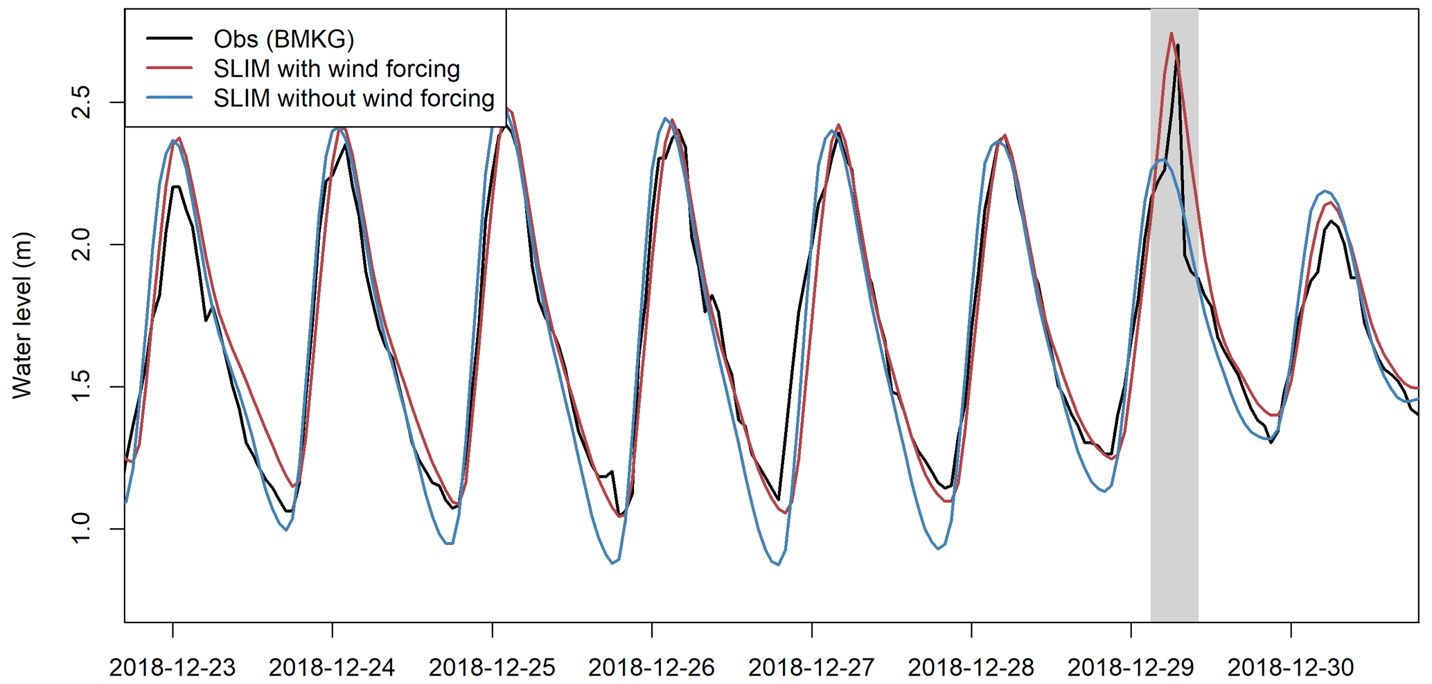
Figure 11 Validation of water level at Pontianak, where the light-grey box depicts the peak of the inundation. BMKG: Badan Meteorologi, Klimatologi, dan Geofisika (Meteorology, Climatology, and Geophysical Agency of Indonesia).

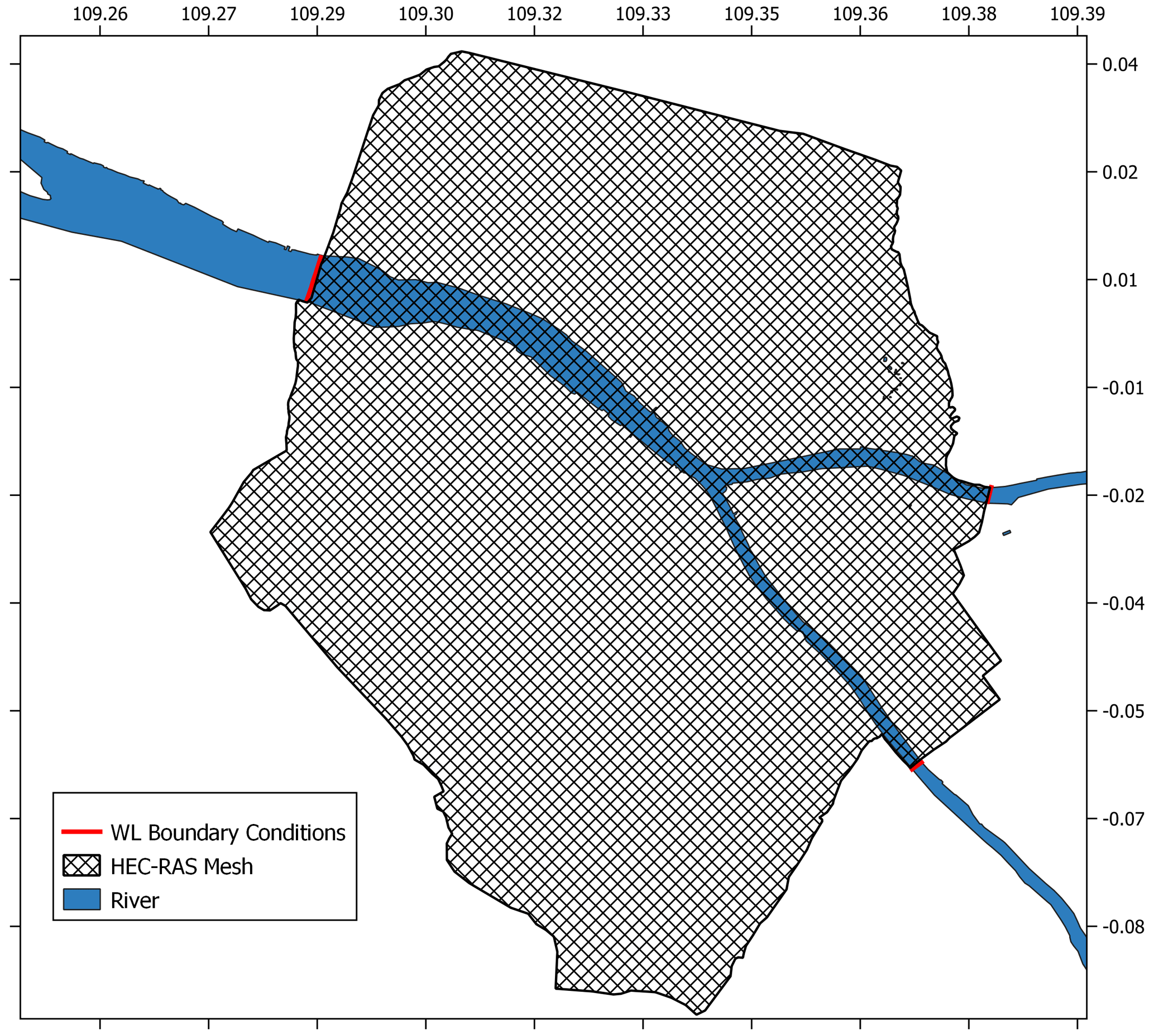
Figure 12 HEC-RAS 2D mesh with a resolution of 10 m for flood extent analysis in the city of Pontianak. WL: water level.

The validation result shows that the NSE is 0.82, indicating that the model has a good performance. The RMSE of its peaks is 0.04 m. These results suggest that the model correctly reproduces the actual hydrodynamic processes. The inundation event on 29 December 2018 is well depicted by the model (light-grey box in Fig. 11). The observational data profile (black) shows that the water level dynamic is at the peak moment during the event, where its peak seems lower than the previous peak period. The water level dynamic is about to go down when suddenly a strong force pushes it to go up again for a short moment. The storm alone is responsible for a 30 cm increase in the water level during this short moment (light-grey box in Fig. 11). After this additional forcing effect disappeared, the water level then decreased steeply and started following the tidal signal again.

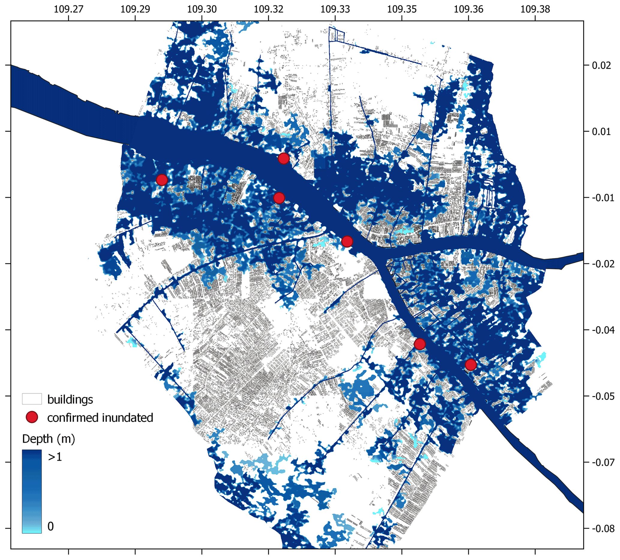
Figure 13 Inundation extent map and its depth during the flood event on 29 December 2018 at 06:00 UTC. The red dots represent places that were reported as inundated during the event. The city's building map was retrieved from OpenStreetMap (https://planet.osm.org, OpenStreetMap contributors, 2021). © OpenStreetMap contributors 2017. Distributed under the Open Data Commons Open Database License (ODbL) v1.0.

A more qualitative validation of the model has also been performed by comparing the extent of the simulated inundation area with observations reported by the local media (Madrosid, 2018). The report mentioned some areas that were confirmed as inundated when the flooding occurred (represented by the red dots in Fig. 13). As a result, our model output validated that these areas were flooded during the flooding event.

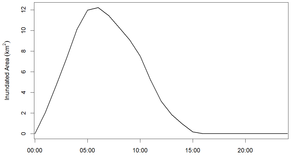
Figure 14 The total inundated area within the city of Pontianak during the flood event on 29 December 2018.

We further investigated the inundation extent and depth over the city of Pontianak using the output of the HEC-RAS model. From the model outputs, we thus know that the extent of this inundation reached lowland within the city located far from the riverbanks (Fig. 13). The overtopped water flooded densely populated areas near riverbanks and propagated much further into the city through the drainage channels. In the western part of the city, floods impacted major areas near riverbanks, while in the eastern part, the major flooded areas fell in lowland areas, located between the Kapuas Kecil and the Landak rivers (district of Pontianak Timur), and portioned the lowland area in the northeast. Next, the peak of the flooding event occurred during a short period. It started at 01:00 UTC, peaked at 06:00 UTC, and finished at 15:00 UTC. At the peak moment, the area inundated was about 12 km² (Fig. 14), in varying depths.

4 Discussion

Based on the discharge scenarios, we found that the city of Pontianak is located in a tidally dominated region. Therefore, the MXWL of the river in the city is not controlled by discharges upstream anymore. Next, we also found that an extreme eastward wind speed with a magnitude greater than 16 m s⁻¹ (the highest wind speed in the Wind_2x scenario) can drive the seawater into the river channels based on the wind surge scenarios. As the storm surge continues to push the water upstream, the pileup water in the estuary will enter the river stream and propagate over several kilometers. If the water propagation is in co-occurrence with high river discharge, the water level can hence overtop riverbanks and lead to a compound inundation over the floodplain. However, if the wind speed is less than 16 m s⁻¹, it does not impact the MXWL profiles. Therefore, the wind speed of 16 m s⁻¹ becomes the minimum wind speed that can drive surges inside the river stream.

On 29 December 2018, rainfall over the city of Pontianak was less than 7 mm so that the effect of excessive rainfall could be ruled out in this event. Meanwhile, an intense wind speed was observed over the coastal area for a few hours. The radar data show cumulonimbus convective clouds formed and moving eastward from the Karimata Strait towards the land (see Appendix Fig. B1). Cumulonimbus is a cloud type that could produce wind surges, tornadoes, and excessive rainfall (Cotton et al., 1992). These clouds reached and covered the Kapuas River's mouth on that date, from 04:30 to 05:25 UTC. Therefore, these clouds most likely triggered a storm over the coastal area with wind speed ranging from 13 to 21 m s⁻¹.

The wind direction was oriented from the west to the east during the event. Hence, the total wind effect became the combination of the direct wind stress effect and the indirect wave run-up effect. Consequently, it drove the water column from the ocean to the western coast of the island of Borneo, where the Kapuas estuary is located. Then, the wind piled up the tidal waters inside the Kapuas River mouth. The piled-up water then propagated upstream from the river mouth and was coincidentally met with an intermediate river discharge. This phenomenon created an increasing water level and caused a short-duration overflow over the floodplain. Therefore, using this scenario, we suggest that the main trigger for the compound flooding, which occurred on 29 December 2018, was an interaction between a storm surge at the estuary area and a medium discharge from the Kapuas River.

As with all modeling studies, there are some limitations related to the model that should be mentioned. Firstly, many different compound flooding schemes possibly occur in this area that have not yet been simulated. Therefore, the delineation of the compound flooding risk zones based on the MXWL proposed for the Kapuas River needs further investigation in the future. Secondly, we have not yet imposed excessive rainfall scenarios in the model so that the model only depicts inundation processes as the effect of the river discharges, tides, and wind surge. In the actual case, a single instance of excessive rainfall is enough to trigger urban flooding over the floodplain area. Next, the computational domain does not cover all of the dry land over the delta. It is only limited to Pontianak and the Kapuas Kecil riverbanks from the city to the river mouth. Consequently, the simulation might not wholly describe the inundation processes and the real extent of the inundated area. These limitations will be improved in future work.

Regarding the event's impact on 29 December 2018, the flooding occurred on a day of low precipitation. Therefore, the residents were not aware and not prepared for such a significant flood event. Even though it happened only for a short period, the economic loss was severe (Madrosid, 2018). Such loss can hopefully be avoided after the local water management agency installs a flood warning system built based on our proposed models.

5 Conclusion

In this study, a model that depicts the Kapuas River's hydrodynamic processes and its interaction with the Karimata Strait tides and wind surges has been successfully set up. We simulated the hydrodynamic processes during extreme events using the model and assessing the impact on the maximum water level along the Kapuas River. We found that wind surges with speeds between 16 and 24 m s⁻¹ over the Kapuas estuary can raise the water level to 150 km upstream. If the wind speed is more than 24 m s⁻¹, then the surge impact can travel further beyond this point. The stronger the wind speed, the further the surge impact will travel upstream. If the surge propagation upstream occurs during intermediate or high river discharges, it can significantly increase the river water level and trigger an inundation over the floodplain, including the city of Pontianak.

Next, based on the maximum water level profiles, we delineate the stream along the Kapuas River into three regions. From the river mouth to about 30 km up the river is the tidally dominated region, where the river discharge levels do not impact the maximum water level anymore. From about 30 to 150 km is the transition region, where the maximum water level is influenced by the interaction between the tides, the surges, and the river discharges. Then, from about 150 km upstream is the river-dominated region, where surges (with wind speed less than 24 m s⁻¹) no longer impact the maximum water level; with- and without-tides scenarios have similar MXWL profiles. The local water management agency can use this zoning category in assessing and mitigating the compound flooding hazard along the riverbanks.

Lastly, as a case study, the factors that drive the inundation event over Pontianak on 29 December 2018 have been successfully investigated. The wind surge, which occurred in the estuary area, was concluded to be the main trigger of the flood event. This wind surge pushed seawater upstream and met with a medium river discharge, therefore triggering a short inundation event over the floodplains, especially the city of Pontianak.

Appendix A: Detail on the tidal constituents

The amplitude, phase, and energy of each tidal constituent at the river mouth and in Pontianak are summarized in Tables A1 and A2.

Table A1 Tide constituents at the Kapuas Kecil River mouth (0.0617^∘ N, 109.1751^∘ E) in December 2018.

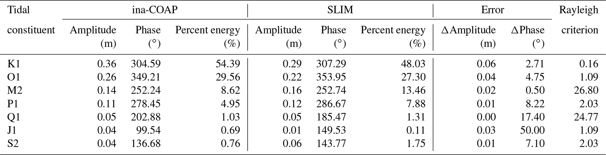
Table A2 Tide constituents in the middle of Pontianak (0.020431^∘ S, 109.33852^∘ E) in December 2018.

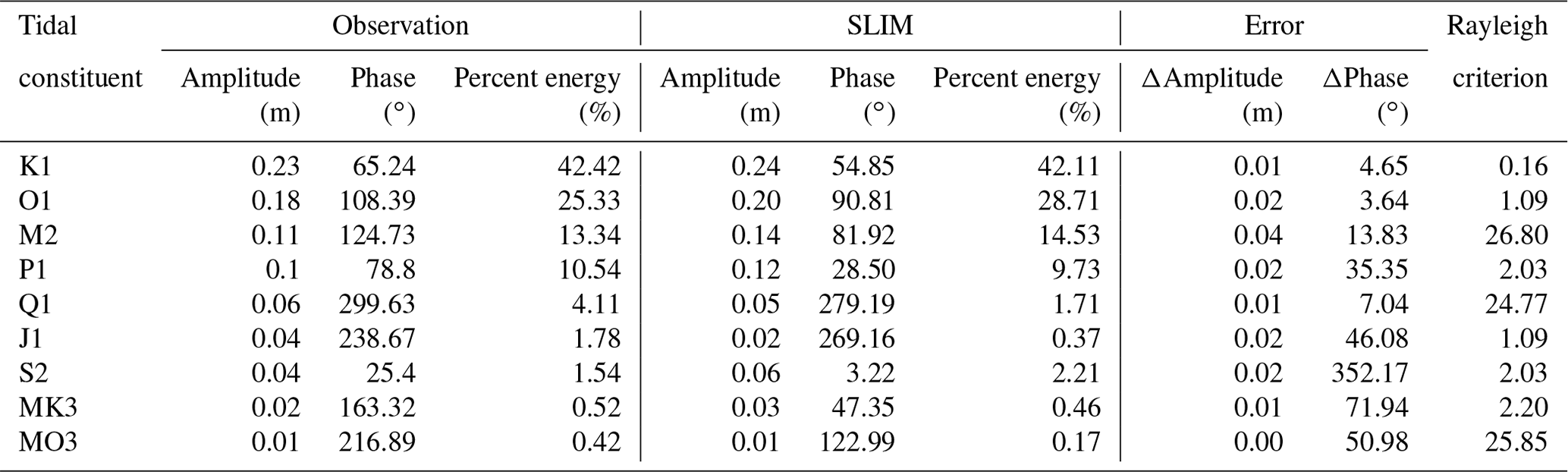
Table A3 Scenarios used to force the model. The simulation duration is 1 whole month, with wind direction varying from 0 to 360^∘, pressure varying from 100.5 to 101.5 kPa, and a tidal range of 1.8 m.

Appendix B: Local weather conditions on 29 December 2018

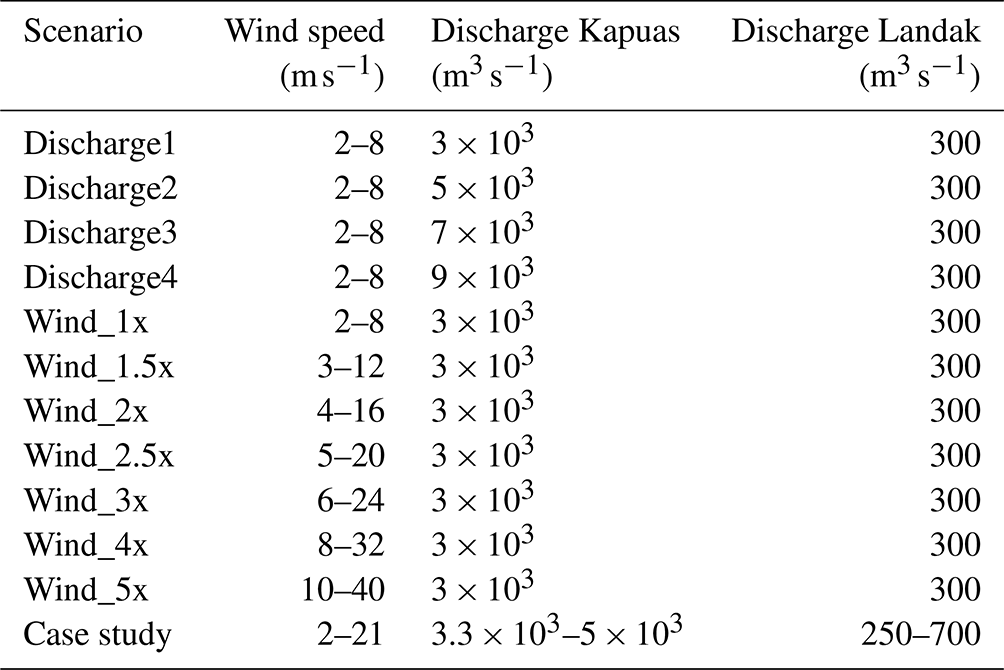
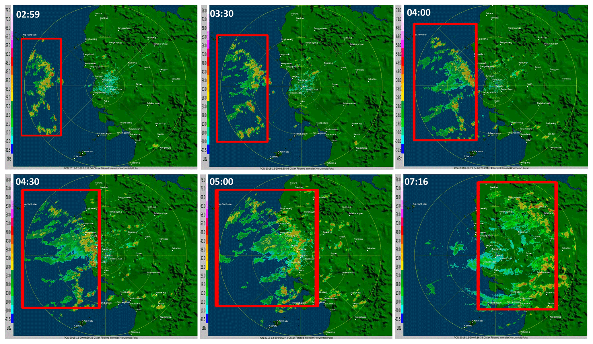
Figure B1 Radar data, observed by the Supadio Meteorological Station (https://kalbar.bmkg.go.id/, last access: 3 April 2021), depict the clouds' growth and movement (in the red box) on 29 December 2018. The clouds started to grow over the ocean and are pushed by the wind to move eastward at 02:59 UTC. The clouds reach their maximum intensity at 05:00 UTC while located above the Kapuas estuary. Furthermore, the clouds spread over a wider area with a weakening intensity at 07:00 UTC.