the Creative Commons Attribution 4.0 License.
the Creative Commons Attribution 4.0 License.
 | 30 Aug 2022
CO2 and CH4 exchanges between moist moss tundra and atmosphere on Kapp Linné, Svalbard
Anders Lindroth
Norbert Pirk
Ingibjörg S. Jónsdóttir
Christian Stiegler
Leif Klemedtsson
Mats B. Nilsson
We measured CO2 and CH4 fluxes using chambers and eddy covariance (only CO2) from a moist moss tundra in Svalbard. The average net ecosystem exchange (NEE) during the summer (9 June–31 August) was negative (sink), with −0.139 ± 0.032 µmol m−2 s−1 corresponding to −11.8 g C m−2 for the whole summer. The cumulated NEE over the whole growing season (day no. 160 to 284) was −2.5 g C m−2. The CH4 flux during the summer period showed a large spatial and temporal variability. The mean value of all 214 samples was 0.000511 ± 0.000315 µmol m−2 s−1, which corresponds to a growing season estimate of 0.04 to 0.16 g CH4 m−2. Thus, we find that this moss tundra ecosystem is closely in balance with the atmosphere during the growing season when regarding exchanges of CO2 and CH4. The sink of CO2 and the source of CH4 are small in comparison with other tundra ecosystems in the high Arctic.
Air temperature, soil moisture and the greenness index contributed significantly to explaining the variation in ecosystem respiration (Reco), while active layer depth, soil moisture and the greenness index were the variables that best explained CH4 emissions. An estimate of temperature sensitivity of Reco and gross primary productivity (GPP) showed that the sensitivity is slightly higher for GPP than for Reco in the interval 0–4.5 ∘C; thereafter, the difference is small up to about 6 ∘C and then begins to rise rapidly for Reco. The consequence of this, for a small increase in air temperature of 1∘ (all other variables assumed unchanged), was that the respiration increased more than photosynthesis turning the small sink into a small source (4.5 g C m−2) during the growing season. Thus, we cannot rule out that the reason why the moss tundra is close to balance today is an effect of the warming that has already taken place in Svalbard.
- Article
(5174 KB) - Full-text XML
-
Supplement
(11707 KB) - BibTeX
- EndNote


Climate warming is predicted to be most evident at high latitudes (Friedlingstein et al., 2006), with profound effects on ecosystem functioning. One of the high-latitude regions that are expected to experience the most dramatic changes caused by climate change is the Arctic. This region, which is located roughly north of the tree line, is characterized by cold winters and cool summers and with mean annual temperatures below zero. The summer periods are short, ranging between 3.5 and 1.5 months from the southern boundary to the north, and July is normally the warmest month. Annual precipitation is generally low, decreasing from about 250 mm in the southern areas to 45 mm in polar deserts in the north (Callaghan et al., 2006).
The permafrost soils in the Arctic store 1035 ± 150 Pg of organic carbon in the top 0–3 m (Hugelius et al., 2014), which is more than the average 2010–2019 of 860 Pg of carbon in the atmosphere (Friedlingstein et al., 2020). The increased warming in these areas can induce higher decomposition rates due to increased microbial activity, which will provide a positive feedback to the climate system (Schuur et al., 2015). On the other hand, warming can also increase photosynthesis and carbon uptake and thus compensate for, or exceed, the effect of increased decomposition. Climate warming is also affecting plant community composition and the length of the growing season (Post et al., 2009), which also has an impact on the processes regulating annual carbon emissions and uptake (Bosiö et al., 2014). There is, however, a large uncertainty regarding the timing, magnitude and possible sign of potential feedbacks caused by these changes (Myers-Smith et al., 2020).
Understanding processes that are controlling the exchanges of greenhouse gases in the Arctic is crucial for the assessment of potential feedback effects. For this purpose, multiple year-round long-term studies including direct measurements of CO2 and CH4 fluxes covering all seasons, winter, spring, summer and autumn, would be ideal. This is a great challenge in the harsh climate of the Arctic and with limited support of key infrastructures for, e.g., provision of electricity for operation of instruments.
In spite of these difficulties, a few year-round studies have been performed during the last couple of decades. In the low Arctic, Oechel et al. (2014) demonstrate the importance of the wintertime fluxes in a tussock tundra ecosystem in Alaska. They found that the non-summer season emitted more CO2 than the corresponding uptake during the summer, resulting in a net source to the atmosphere of about 14 g C m−2 on an annual basis. They also showed that the shoulder seasons, spring and autumn, roughly outweighed the summer uptake. Euskirchen et al. (2012, 2017) measured net CO2 exchange in three different tundra ecosystems: heath tundra, tussock tundra and wet sedge tundra in northern Alaska over 3 years. They found that the uptake of −51 to −95 g C m−2 during the summer (June–August) was overturned by the respiration that occurred during the winter period, resulting in net annual losses for all three ecosystems. Zhang et al. (2019) reported 5 years of year-round flux measurements in a heath ecosystem on west Greenland, and they found that the heath was an annual sink of −35 ± 15 g C m−2. One year with an anomalously deep snowpack showed a 3-fold higher respiration during the winter as compared to the other years, which resulted in a significantly lower net uptake during that year.
Even fewer studies have been done on year-round studies in the high Arctic. Lüers et al. (2014) quantified the annual CO2 budget using eddy covariance measurements in a river catchment area near Ny-Ålesund on Spitsbergen in the Svalbard archipelago, and they found that the ecosystem was in C balance. The footprint area was a semi-polar desert with only 60 % vegetation cover and patches of bare soil and stones. Also in Svalbard but further south in Adventdalen on a flat alluvial fen irregularly covered with ice wedged polygons, Pirk et al. (2017) made year-round measurements of CO2 fluxes and found it to be a net sink of −82 g C m−2. Because of the irregularities caused by the ice wedges and the differences in wetness, they focused the analyses on the spatial variability in two different directions, one wetter and one drier, and they estimated the annual net ecosystem exchange to −91 and −62 g C m−2 for the respective areas.
The Arctic ecosystems constitute also a source of CH4 to the atmosphere even if it is not a very large one. Saunois et al. (2020) estimated that the northern high-latitude region (60–90∘ N) contributed 4 % of global emissions, and emissions from wetlands are only part of the emissions from this region. However, in the light of the vulnerability of the high-Arctic permafrost areas and considering the large carbon pool and the predicted changes in climate, a quantification and understanding of CH4 exchanges in these areas are still important. Christensen et al. (2004) showed one example of a dramatic impact of the climate warming on the CH4 emissions in a permafrost mire in sub-Arctic Sweden. The warming which has been visible in this area for decades and its impact on permafrost and vegetation changes were estimated to have caused an increase in landscape CH4 emissions in the range 22 %–66 % in the period 1970–2000.
Mastepanov et al. (2008) were the first to show the importance of emissions also outside of the growing season. They observed a large burst of CH4 from a fen area in Zackenberg, Greenland, after the growing season and during the time when the soil started to freeze. This finding was confirmed in a later paper (Mastepanov et al., 2013), and the process was hypothetically attributed to the subsurface CH4 pool. Hydrology and vegetation composition play an important role for CH4 emission and dynamics. McGuire et al. (2012) made a comprehensive summary of CH4 exchanges of the Arctic tundra showing the difference between wet and dry ecosystems; the wet tundra emitted 5.4 to 13.0 g CH4-C m−2 during summer and 8.5 to 20.2 g CH4-C m−2 annually. The corresponding values for the dry/mesic tundra were 0.3 to 1.4 and 0.3 to 4.3 g CH4-C m−2, respectively. Bao et al. (2021) utilized year-round measurements of CH4 fluxes from three sites of the AmeriFlux network in northern Alaska to demonstrate the importance of the spring and autumn seasons for the annual emission. The shoulder seasons contributed about 25 % of the annual emissions, and the autumn season had about 3-times-higher emissions than the spring season. These findings increasingly emphasize the importance of year-round measurements to fully understand the CH4 controls and dynamics.
The main aim of this study is to provide another piece of the puzzle concerning CO2 and CH4 exchanges from different but widespread ecosystem types in the high Arctic. We hypothesize that this moist tundra ecosystem is a net carbon sink during the growing season and that the summer emissions of methane will be at levels comparable with other methane-emitting high-Arctic ecosystems. We made flux measurements of CO2 and CH4 in an moist moss tundra ecosystem situated at Kapp Linné on the west coast of the Svalbard archipelago in 2015 and with an additional campaign in 2016. The measurements in 2015 were done using both the eddy covariance system (CO2) and chambers (CO2 and CH4) but only chambers in 2016. We quantify ecosystem respiration (Reco), gross primary productivity (GPP) and net ecosystem exchange (NEE) during the growing season based on a combination of chamber and eddy covariance measurements. The CH4 emission was only quantified for the summer season. We also analyze the environmental controls of the fluxes.
Research site and measurements
This study was performed in the Svalbard archipelago near the weather station Isfjord Radio (78∘03′08′′ N, 13∘36′04′′ E; altitude 7 m), which is located right on the foreland of Kapp Linné on the island of Spitzbergen (Fig. S1). The tundra area where the measurements were performed is located about 1 km southeast of the station. The study area consists of moist moss tundra, a widespread ecosystem in Svalbard (Vanderpuye et al., 2002; Ravolainin et al., 2020). The vegetation is characterized by the moss species Tomentypnum nitens, Sanionia uncinata, and Aulacomnium palustre and a sparse cover of vascular plants (20 %–40 %), dominated by Equisetum arvense, Salix polaris and Bistorta vivipara. Other vascular plant species were found in the plots: Saxifraga cespitosa, Saxifraga oppositifolia, Silene acaulis, and some grass species, most likely Alopecurus ovatus (previously A. borealis) and Poa arctica. The vegetation analysis was made from photographs of chamber location plots taken between 26 June and 2 July 2015 (see Fig. S4a–y in the Supplement).
The net ecosystem exchange of CO2 was measured with an eddy covariance (EC) system located centrally on the moss tundra (78∘03′28.6′′ N, 13∘38′40′′ E). The sonic anemometer (USA-1; Metek GmbH, Germany) was mounted on top of a tripod (see Fig. S1) at 2.7 m height. The CO2 and H2O concentrations were measured with an open-path sensor (LI-7500; Li-Cor Inc., USA) placed just beneath the sonic anemometer and inclined about 30∘ pointing towards the east. Radiation components, incoming and outgoing shortwave and longwave (CNR-4; Kipp and Zonen, the Netherlands), were measured at 2.0 m height above the ground with the sensor directed towards the south. All sensors were connected to a data logger (CR-1000; Campbell Scientific, USA) which was powered by a solar panel and a battery. The EC sensors were sampled and stored at 10 Hz, and all other sensors were sampled at 0.1 Hz with storage of 30 min mean values. These measurements were made from 25 June to 17 September 2015. The total data coverage during this period was 47 %, with a longer break in the measurements between 28 July and 29 August. The impact of substantial gap filling of measured EC data and partial modeling in order to complete the full growing season is further discussed below.
The soil efflux of CO2 and CH4 was measured with a dark chamber connected to a gas analyzer (Ultraportable Greenhouse Gas Analyzer; Los Gatos Research, USA) on 24 locations within the EC average footprint area. A circular thin-steel frame, 15 cm in diameter and 15 cm high, was inserted ca. 5 cm into the ground in each location. The sharp edge of the frames made it easy to insert them into the ground without damaging the vegetation and with minimal soil disturbance. A picture was taken of each frame (see Supplement) for documentation of vegetation and for calculation of different indexes. The chamber was also made from steel, and it had a rubber seal in the end facing the frame (Fig. S2) to make it airtight when mounted on the frame. The volume of the chamber and the part of the frame raised above the surface was 5.3 L. A small fan was installed inside the chamber to provide good mixing of the air during measurement. A small weight (stone) was placed on top of the chamber during measurement to prevent it from moving due to wind gusts. During concentration measurement air was circulated in a closed loop between the chamber and the gas analyzer in ca. 10 m long, 4 mm diameter polyethene tubes (see Fig. S2). The airflow through the analyzer was ca 1.2 L min−1. The chamber was ventilated in the free air about 1 min before each measurement, which lasted for 5 min. The concentrations were recorded and stored once per second by the gas analyzer. The time stamp of the recorded data was used to identify measurement cycles for analysis of fluxes.
The chamber measurement positions were selected in the following way. The frames were grouped in two sections, one northeast and one southwest of the flux tower, since it was expected that the main wind direction would be along that direction. Each group was then split into three subsections with four measurement points within each one of them. The locations were named S1:1–S1:4, S2:1–S2:4, S3:1–S3:4, N1:1–N1:4, N2:1–N2:4 and N3:1–N3:4. The four measurement points within each subsection were then placed along a transect with 3–4 m between each point. This way it was possible to measure all four chamber locations without having to move the whole measurement system. Chamber measurements were made in three separate campaigns: mid-summer (26 June to 2 July 2015), late summer (25–27 August 2015) and early summer (14–15 June 2016). Each location was measured three times during each one of the three campaigns – a total of 216 measurements. Besides gas concentrations, also soil temperature (5 cm), soil moisture (0–5 cm) and active layer depth were measured during each campaign.
Meteorological data needed for analyses and gap filling were obtained as follows: hourly air temperature and relative humidity from Isfjord Radio, half-hourly global radiation from Adventdalen, daily snow depth and ground ice conditions from Svalbard Airport, and monthly precipitation from Isfjord Radio and Barentsburg. The distances between the measurement site and these stations are as follows: Isfjord Radio, 1 km; Barentsburg, 13 km; Svalbard Airport, 46 km; and Adventdalen, 50 km. Using data from the more distant locations, Svalbard Airport and Adventdalen, introduces some additional uncertainty. Concerning global radiation data, we could compare in situ-measured half-hourly radiation with the corresponding data from Adventdalen for a shorter period, and it showed general good agreement although with relatively large scatter (; r2=0.57; n=580). According to Dobler et al. (2021) the amount of precipitation in the area where Kapp Linné and Svalbard Airport are located does not show any significant differences on an annual basis. Vickers et al. (2020) analyzed timing of snow cover in Svalbard, and they showed that the mean (2000–2019) first snow-free day is very similar in areas where Kapp Linné and Svalbard Airport are located. Thus, we are confident that using data from these relatively remote locations does not introduce serious bias in our analyses. Data sources are given in the Acknowledgements.
The raw data from the eddy covariance flux measurements were analyzed using the EddyPro software version 6.1.0 (Li-Cor, 2016). A correction was made for the impact of the additional heat flux in the sensor path of the open-path analyzer on the flux calculations according Burba et al. (2008). Gap filling during the measurement period was made using the REddyProc online eddy covariance data processing tool developed at the Max Planck Institute for Biogeochemistry (Wutzler et al., 2018) without u* correction since we could not identify any threshold for u*. The u* threshold is generally low for low and smooth vegetation (Pastorello et al., 2020), and for a wind-exposed site like ours, it is not surprising that such threshold could not be found. Flux partitioning was made with the daytime-based method according Lasslop et al. (2000). Only data of highest quality, i.e., class = 0, were retained for the gap filling and further analyses. Gap filling outside of the EC measurement period to obtain the carbon balance for a full growing season was made by modeling using the Lloyd and Taylor (1994) model for Reco and an empirical light response function for GPP (see below). The measured respiration by chambers was used to obtain the parameters for Reco, and EC data were used for fitting of the light response function for GPP.
For flux footprint calculations the roughness length (z0) is needed, and it was calculated from the wind profile relationship in near-neutral () conditions:
where zm is measurement height, u(z) is wind speed at height z, k is von Karman's constant and u* is friction velocity. We used the flux footprint prediction (FFP) online tool by Kljun et al. (2015) to calculate the footprint climatology.
The fluxes from the chamber measurements were estimated from the time change of the concentrations using linear regression. Every individual measurement was inspected and evaluated manually. These inspections showed that 50 s for CO2 and 100 s for CH4 were optimal to obtain near perfectly linear responses a few seconds after the chamber had been placed on the frame. The slopes of the regressions were then used to calculate fluxes per unit surface area. The flux detection limits for CO2 and CH4 were calculated in the following way: first the peak-to-peak variations in the respective gases were determined when the chamber was ventilated in the free air and when conditions were steady. Then 20 sets of artificial “fluxes” for each gas species were estimated based on 100 randomly generated concentrations for each data set. The peak-to-peak difference was used as seed (input) for the randomly generated values. The 95 % value of the distribution of these randomly generated fluxes was taken as the flux detection limit for the respective gas.
The pictures of the vegetation inside of the chamber frames were analyzed using the ImageJ (https://imagej.net, last access: 29 December 2020) public domain software. The camera color channel information (digital numbers for red (R), green (G) and blue (B) channels) was collected from the JPEG pictures. This type of picture is for instance used in studies that are tracking the phenological development of vegetation (e.g., Richardson et al., 2009). The so-called green index (GI) is applied to detect differences in greenness of vegetation:
This index was also estimated for the central footprint area (100 m radius) of the flux measurement location using a picture taken at 160 m above the altitude of the measurement area.
Forward stepwise linear regression (SigmaPlot 12.5) was used to analyze the dependency of the CO2 and CH4 fluxes on environmental variables. We tested for air temperature (Ta), soil moisture (θ), soil temperature (Ts), active layer depth (ALD), measurement location (Sid) and GI.
For gap filling of Reco we only had access to air temperature with full annual coverage, and, thus, we could only use this driver for estimation of the Reco. The measured chamber CO2 fluxes were fitted to the Lloyd and Taylor (1994) model with air temperature (Ta) as an independent variable:
During the EC measurement period (25 June to 17 September 2015) the GPP was estimated as
where NEEf is the gap-filled NEE according to Wutzler et al. (2018). This way Reco and GPP become consistent with the measured and gap-filled NEE. For the time before and after this period, NEE was estimated as the sum of modeled Reco and modeled GPP. The data for the GPP model was derived from
where NEEm is the measured net ecosystem exchange. The GPPm was then fitted to a light response function:
For CO2 exchanges and partitioning we combined the soil efflux measurements with the chamber system with the eddy covariance flux measurements. This was crucial for the partitioning and for gap filling because from 20 April to 20 August at this location the sun is above the horizon 24 h of the day, and this means that there were few occasions of dark nighttime measurements with the eddy covariance system, and all of these were collected at the very end of the summer. We consider the chamber measurements that were distributed across the summer to be more representative of Reco for this location.
For CH4 exchanges we do not have any eddy covariance measurements, so we present only chamber data for this variable.
4.1 Weather
The mean annual temperature at Kapp Linné was −1.5 ∘C during 2015, which was 3.5 ∘C higher than the long-term mean (1961–1990) of −5.1 ∘C. The summer (June–August) mean of 5.5 ∘C was 2.0 ∘C higher than the long-term mean for the same time period (Fig. 1). The summer precipitation in 2015 was much lower, 58 mm as compared to the long-term precipitation, which was 121 mm. The annual precipitation was also lower, 431 mm compared to the long-term precipitation, which was 514 mm.
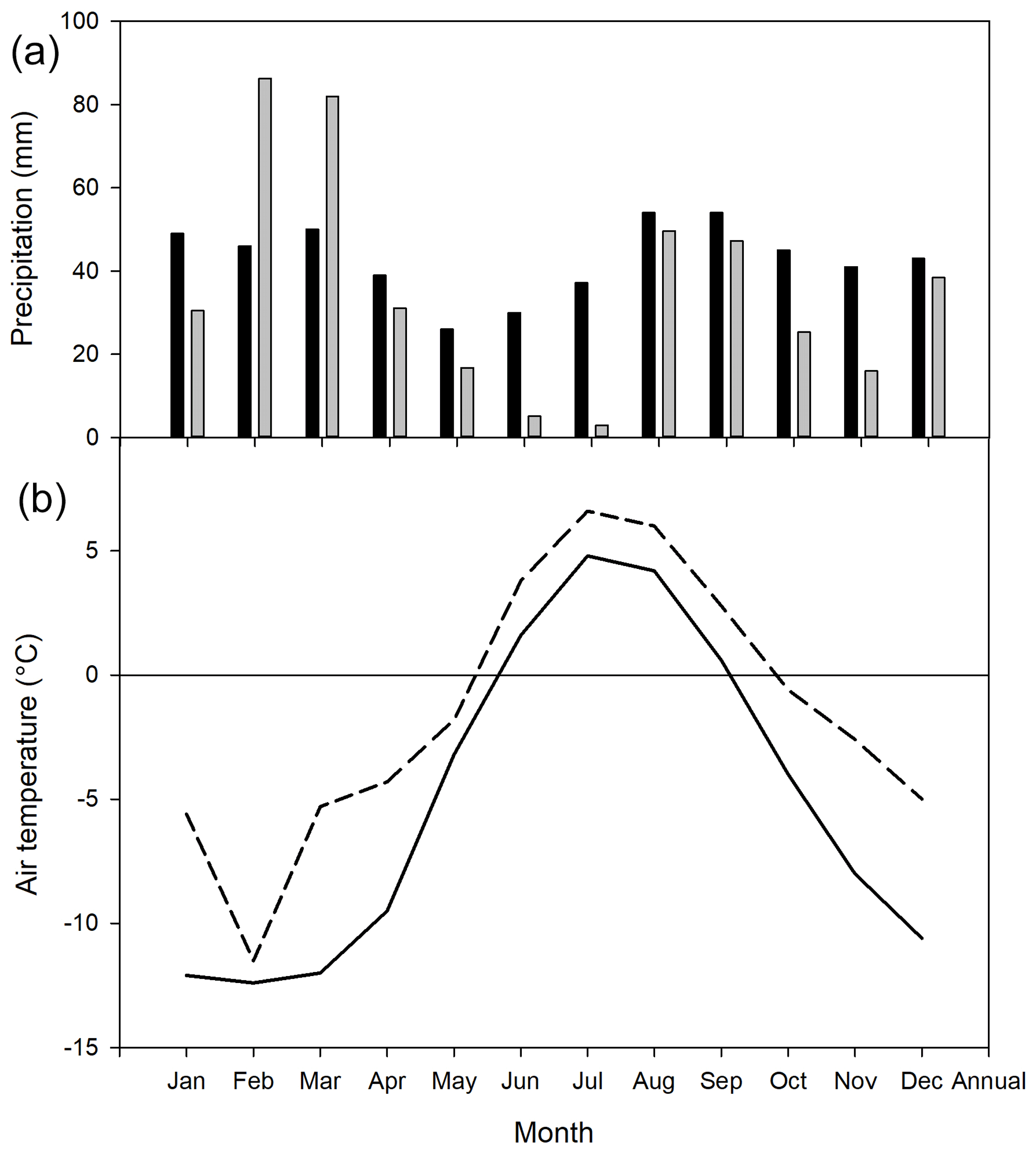
Figure 1Monthly precipitation (a): long-term average 1961–1990 shown by black bars and 2015 by grey bars. Data from Barentsburg for January–May and from Isfjord Radio for June–December. Mean monthly air temperature (b): solid line is long-term average 1961–1990 and dotted line is 2015. Data from Isfjord Radio, which is located about 1 km west of the investigation area.
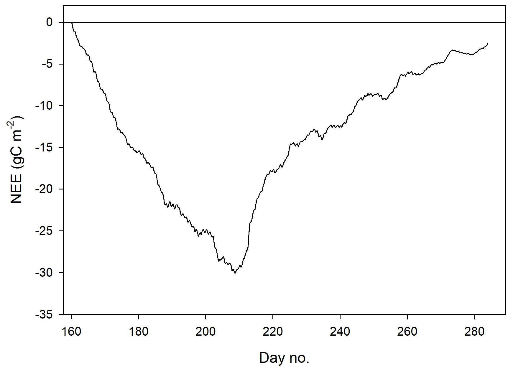
We defined the growing season (the period during which vegetation is photosynthesizing) based on the permanence of the snow pack, which resulted in start day no. 160 and end day no. 284 (Fig. 2). The summer period which normally is defined as June through August was here defined as lasting from 9 June (same as the start of the growing season) until the end of August (Fig. 2).
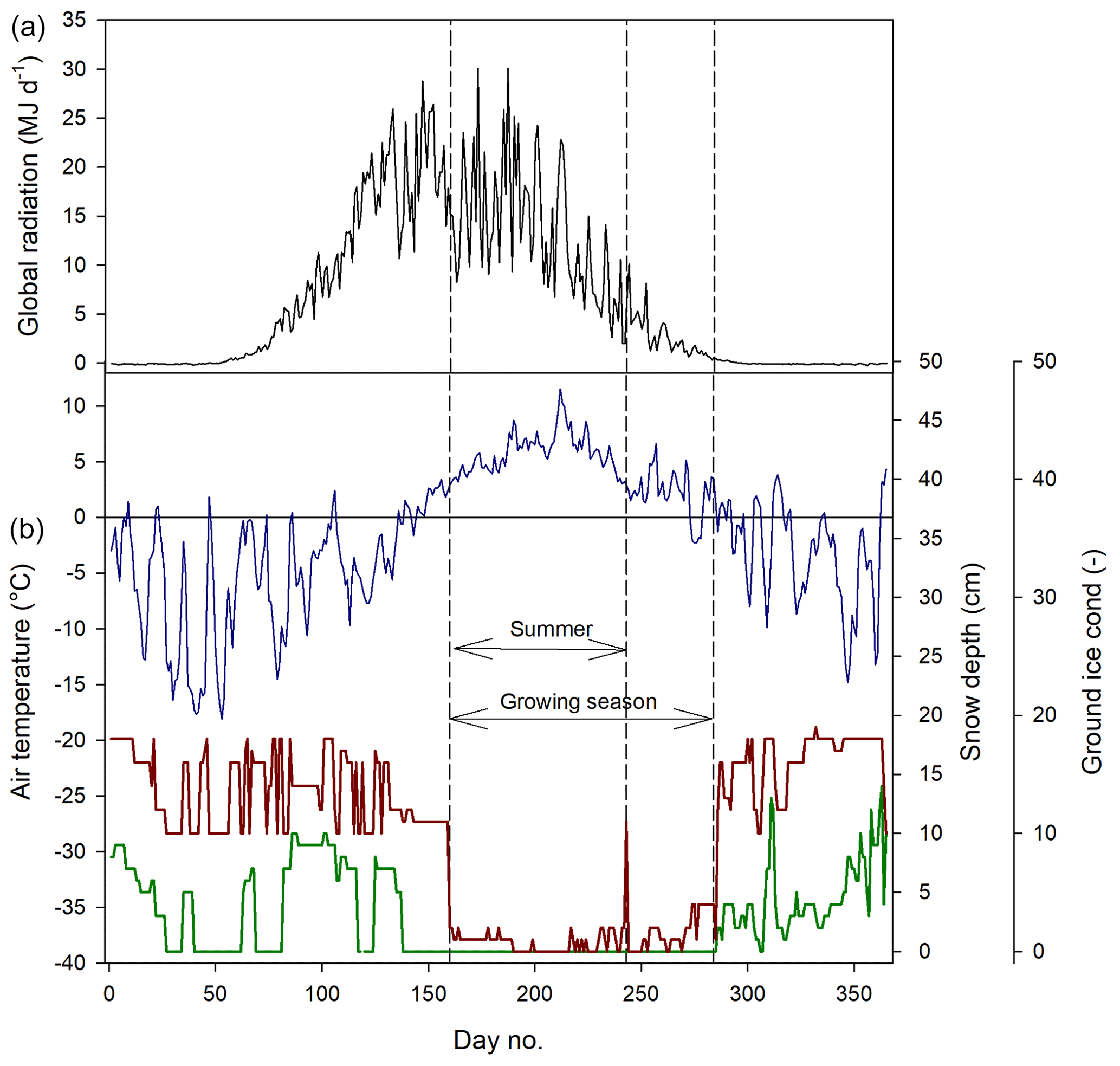
Figure 2Weather conditions during 2015. (a) Mean daily global radiation at Adventdalen. (b) Mean daily air temperature at Isfjord Radio (blue), snow depth (red) and ground ice conditions (green) at Svalbard Airport close to Longyearbyen. The ground ice condition is scaled from 0–20, where 0 is no snow or ice on the ground and 20 indicates a complete cover of snow or ice.
4.2 Flux footprint and greenness
The footprint climatology shows a good representativity of the moss tundra surface by the EC measurements, with 60 %–70 % of fluxes emanating from areas well within the border of the tundra (Fig. 3). The mean green index for a circular area with radius of 100 m centered at the flux tower was 0.34, which corresponded exactly to the mean value for all chamber locations. The GI for the 24 chamber locations varied between 0.316 and 0.369. We observed a good (visual) correlation between GI and coverage of green plants (see Fig. S4a–y of chamber location pictures and GI).
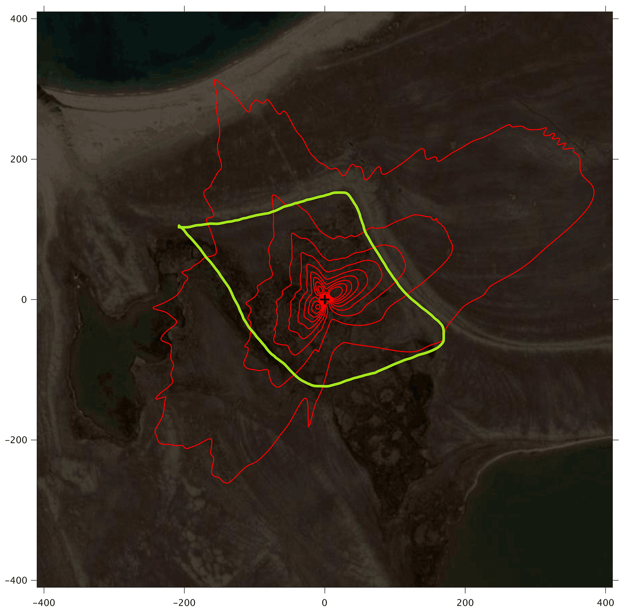
Figure 3The footprint climatology with red contour lines 10 %–90 %. The area within the green line marks the heart of the moss tundra. The scale (m) is shown on the outer borders of the picture (map source: https://Bing.com, Maxar Technologies).
4.3 CO2 exchanges
The CO2 fluxes from the chamber measurements showed quite large variation over time (Fig. 4) and across sampling locations (Fig. 5). The mean CO2 flux of all samples was 0.81 ± 0.11 µmol m−2 s−1. The uncertainty is given as the 95 % confidence limit.
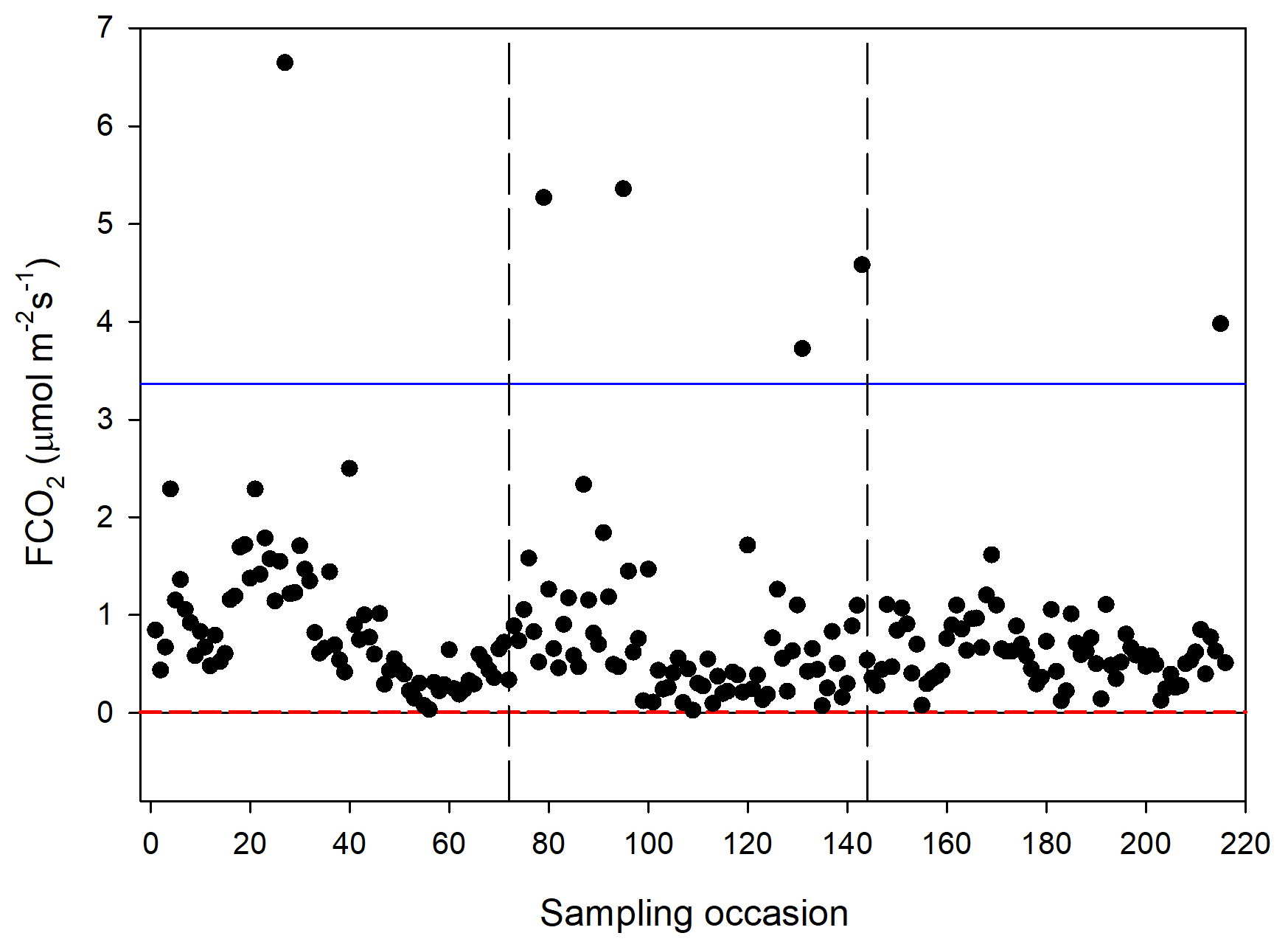
Figure 4Measured CO2 exchange (FCO2) from the 24 sampling points using a dark chamber and portable gas analyzer. The dashed red line indicates the CO2 flux detection limit, and the blue line represents 3 × SD of all data points. The dashed vertical lines separate sampling periods from left to right: 14–15 June, 26 June–2 July and 25–27 August, respectively.
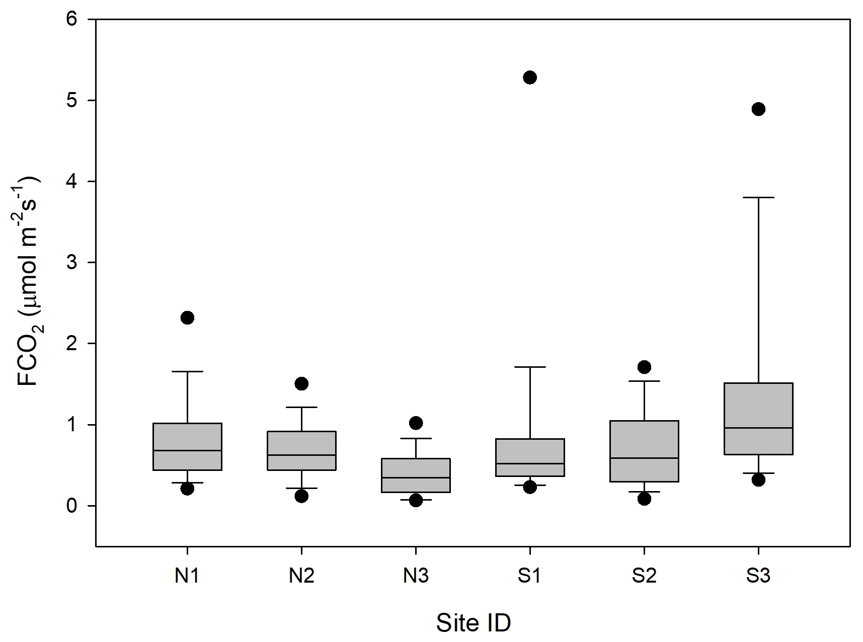
Figure 5Box plot of CO2 fluxes (FCO2) per sampling location named N1–N3 and S1–S3. The boundaries of the grey boxes represent the 25th and 75th percentiles, the line represents the median, and whiskers above and below the boxes indicate the 10th and 90th percentiles. Outlying points are also shown.
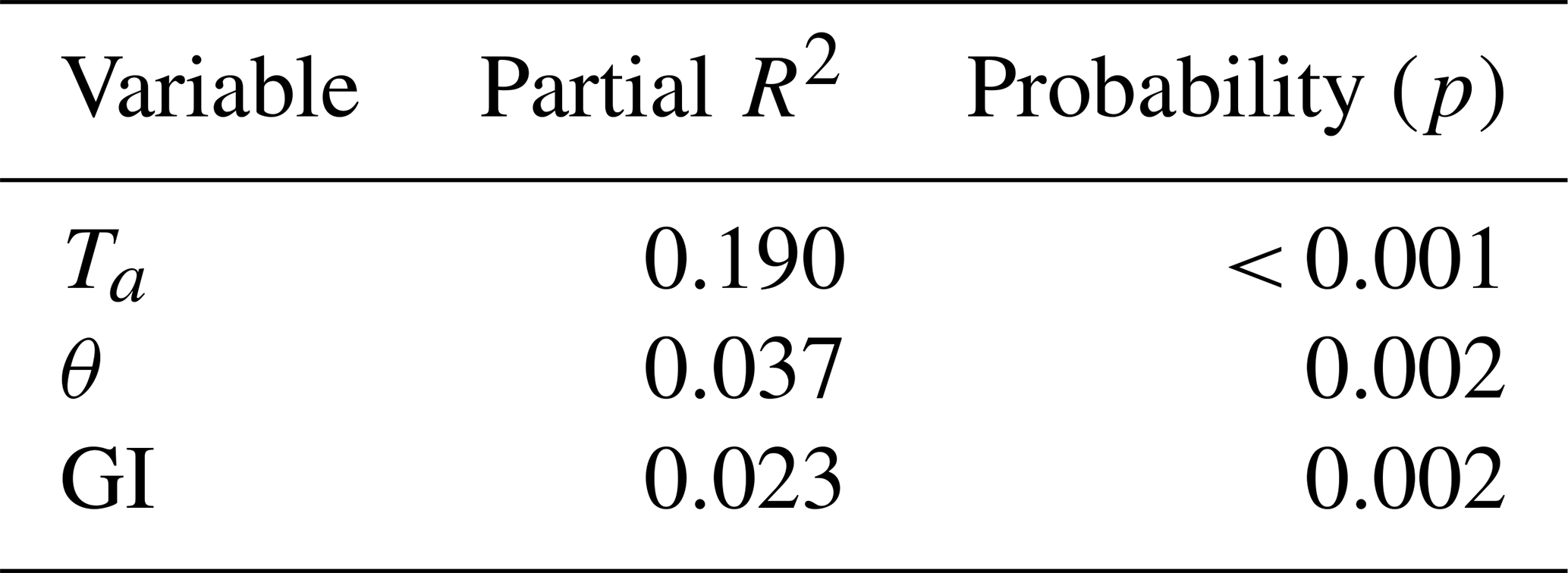
Of the tested environmental variables – Ta, θ, Ts, ALD, Sid and GI – it was only Ta, θ and GI that contributed positively and significantly in decreasing order to explaining the variability of the CO2 flux (Table 1).
Table 1Result of stepwise linear regression with CO2 flux as a dependent variable. The normality test failed, but significance in all variables was confirmed with Wilcoxon signed-rank tests. Ta is air temperature, θ is soil moisture and GI is the green index.
Ideally all of these variables should be used in a model to estimate Reco for gap-filling purposes, but we could only use air temperature since this was the only variable that we had access to with complete coverage for a full year. The Lloyd and Taylor model (Eq. 3 and Fig. 6) was thus used to estimate ecosystem respiration for 2015 using half-hourly air temperature as input.
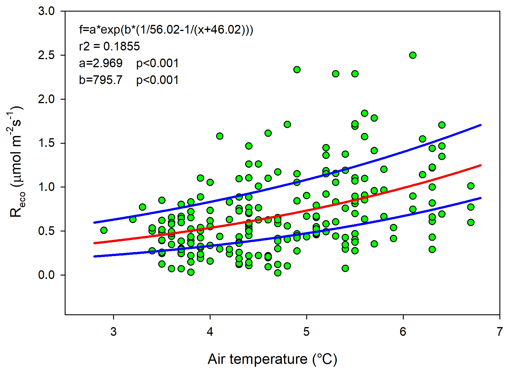
Figure 6Measured ecosystem respiration (Reco; green dots) using chambers plotted against air temperature. The red curve is the fitted equation, and the blue curves are the corresponding boundaries when considering the standard deviation of the parameters.
The modeled gross primary productivity (Eq. 6; GPPm) had a small offset when global radiation was zero (Fig. 7). This offset was adjusted for when the model was applied for gap filling so that GPP becomes zero during nighttime.

Figure 7Gross primary productivity (GPPm) plotted against global radiation (Rg); red symbols are estimated values according to Eq. (5), and the black symbols are the fitted model.
The diurnal course of NEE during June–August exhibits the normal pattern with a successively increasing drawdown of CO2 during the first half of the day, resulting in a maximum around noon. It should be noted that during June until 20 August the sun was over the horizon 24 h, thus no dark period. The positive values at the beginning and end of the diurnal courses are a result of Reco being larger than GPP. As pointed out in Fig. 8, most of the data of August were gap filled, causing some additional uncertainty. However, the diurnal course seems reasonable although the peak during noon is much lower as compared to July. This can be explained by the much lower incoming radiation in August as compared to July; the mean global radiation in July was 192 and 98 W m−2 in August. The mean air temperature was similar during July and August. In September the incoming radiation is very low, and thus GPP is also very low, which results in a NEE that is dominated by the Reco. The positive NEE values around midnight during June–September are in good accordance with the values from the independent dark chamber measurements (Fig. 5).
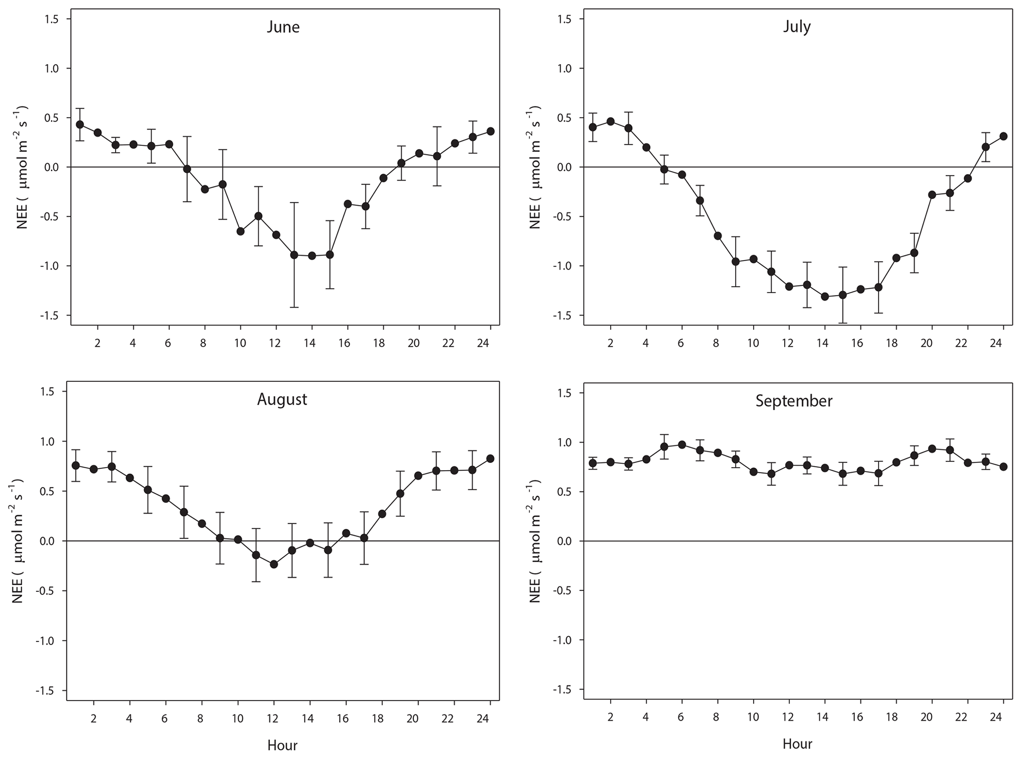
Figure 8The mean monthly diurnal course of net ecosystem exchange (NEE) during the period of eddy covariance measurements 25 June to 17 September. The error bars (every 2nd shown) are the 95 % confidence interval. Notice that the main part of August was gap filled because of measurement problems.
In order to assess the impact of the large gap in measured data in August where we only had 2 d of measured fluxes at the end of the month, we made a comparison between the gap-filled diurnal course based on Wutzler et al. (2018) and our modeling using Eqs. (3) and (6). The results show very good agreement between the two methods (see Supplement), giving support to the realism and reliability of the gap-filled data.
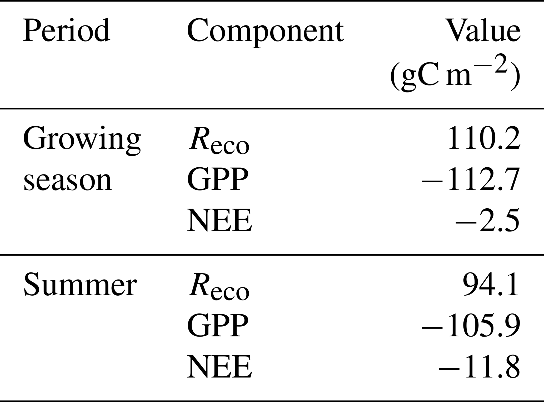
The mean net CO2 flux during the growing season was −0.019 ± 0.024 µmol m−2 s−1, with uncertainty given as the 95 % confidence limit. The cumulated NEE during the growing season ended up negative, with −2.5 g C m−2 (Fig. 9). The mean net CO2 flux during summer was −0.139 ± 0.032 µmol m−2 s−1 (95 % confidence limit), and the cumulated NEE was −11.8 g C m−2 (Table 2).
Table 2Summary of seasonal C fluxes from Kapp Linné. Reco is ecosystem respiration, GPP is gross primary productivity and NEE is net ecosystem exchange.
4.4 Temperature sensitivity of Reco and GPP
The temperature sensitivity of the Reco is already given by the fitted Lloyd and Taylor (1994) equation. In the absence of long time series of measurements during multiple year were natural climate variability could be used to assess temperature sensitivity of GPP, we approached this problem in the following way. We normalize GPP for its dependence on radiation by estimating the difference between the “measured” GPP and the model which only depends on radiation (see Fig. 7). A stepwise linear regression with normalized GPP as a dependent variable and air temperature, time of season, and vapor pressure deficit as independent variables showed that of the total explained variance, air temperature stood for 94 % and time of season and and vapor pressure deficit for 3 % each. Thus, the resulting normalized GPP shows effectively a dependence on air temperature (Fig. 10), with values becoming more negative, i.e., showing increasing GPP with increasing temperature. We fitted the same type of model to these data as for the Reco to be able to compare sensitivities to temperature.
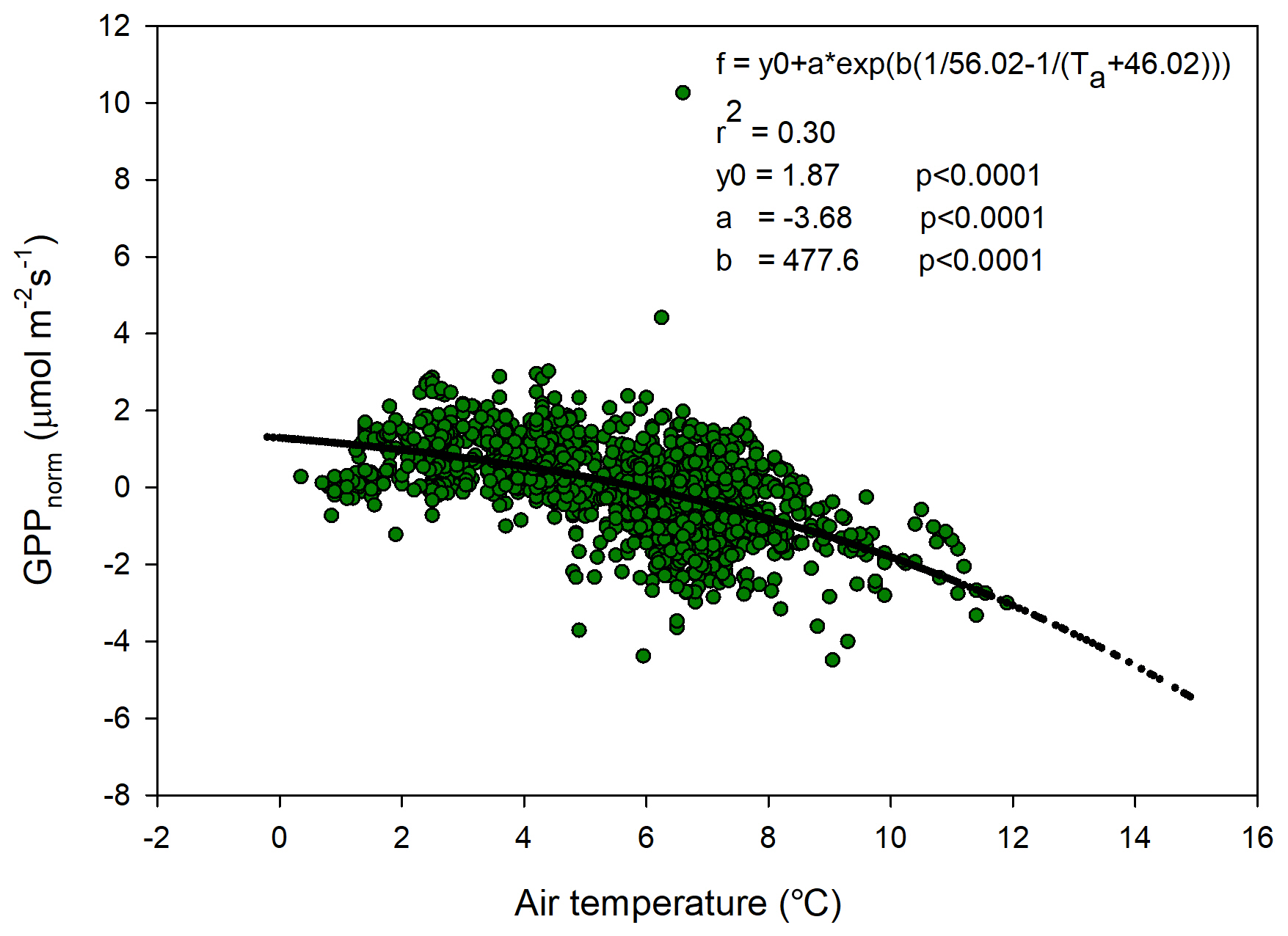
Figure 10Normalized gross primary productivity (GPP) plotted against air temperature and with the fitted exponential model.
In Fig. 11 we reversed the sign of the GPP temperature response function to make it more easily comparable with the Reco response model. The temperature sensitivity (µmol m−2 s−1 K−1) can be estimated from the slope of these curves, and the sensitivity is slightly higher for GPP than for Reco in the interval 0–4.5 ∘C; thereafter, the difference is small up to about 6 ∘C and then begins to rise rapidly for Reco. We tested what impact this could have by increasing the measured half-hourly air temperature by 1 ∘C and found that during the growing season the GPP increased by −31.9 g C m−2 and Reco by 36.4 g C m−2. Thus, a slightly larger increase in Reco as compared to GPP results in the small sink of −2.5 g C m−2 turning into a source of 4.5 g C m−2.
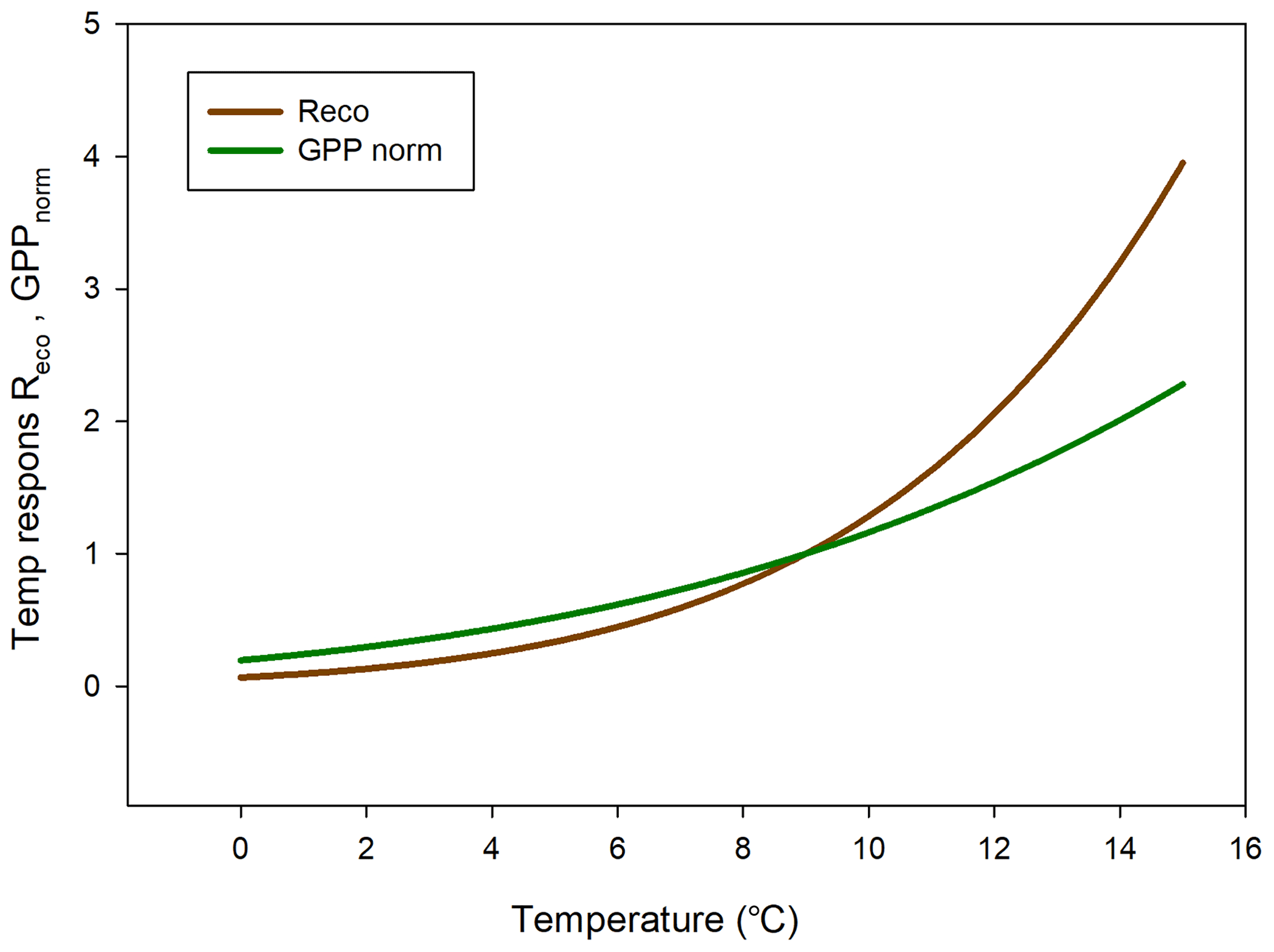
Figure 11Temperature sensitivity for ecosystem respiration (Reco) (brown) and Rg-normalized (positive) gross primary productivity (GPP) (green).
4.5 CH4 exchanges
The CH4 fluxes from the chamber measurements showed large variation over time (Fig. 12) and across sampling locations (Fig. 13). The mean CH4 flux of all samples was 0.00051 ± 0.00024 µmol m−2 s−1. The uncertainty is given as the 95 % confidence limit. Setting all fluxes that fell within the flux detection limits to zero changed the mean value with −0.2 %. Assuming that the mean flux was representative for the whole of growing season 1, the total CH4 summer emission was 0.039 to 0.164 g CH4 m−2.
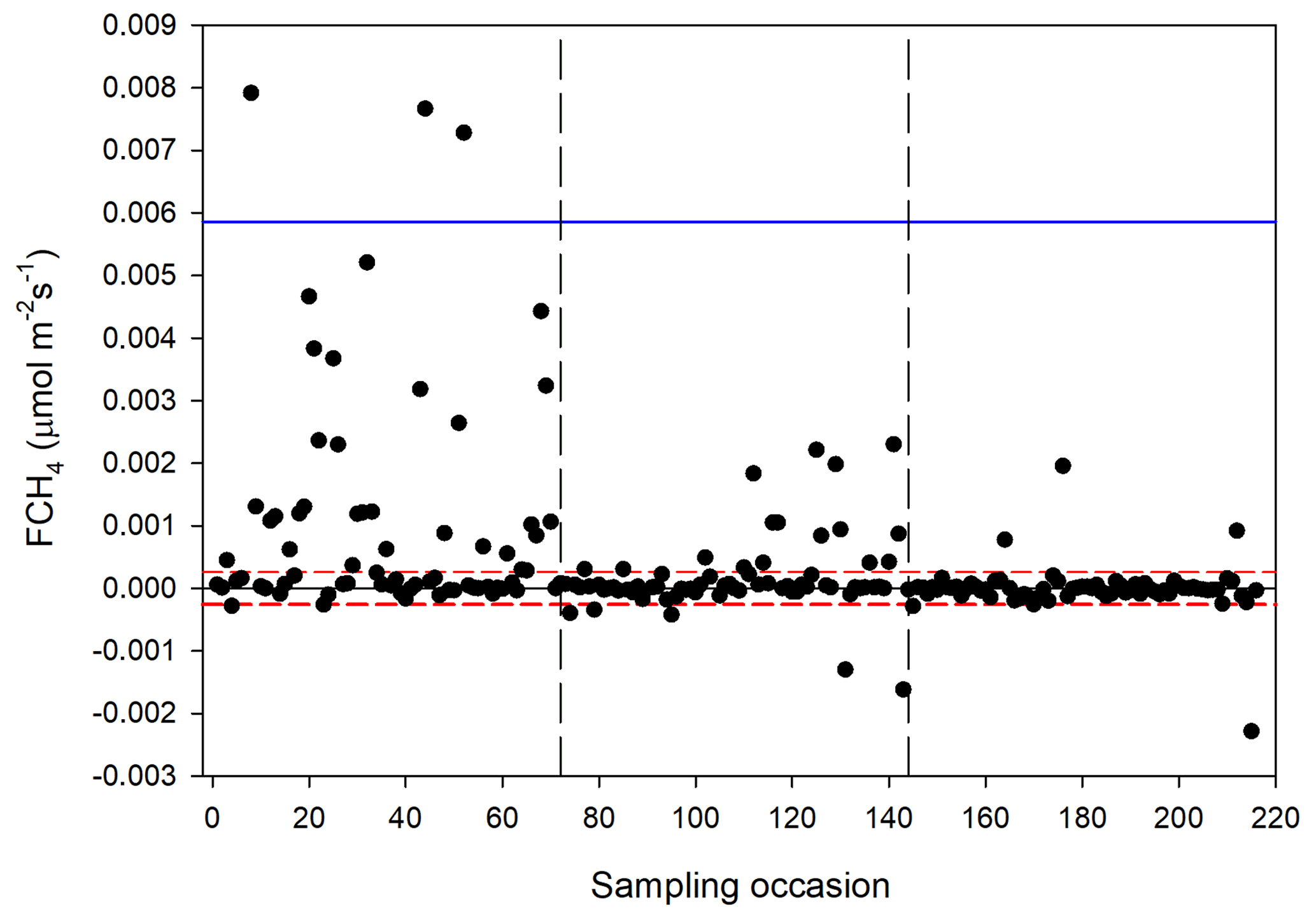
Figure 12Measured CH4 exchange (FCH4) from the 24 sampling points using a dark chamber and portable gas analyzer. The dashed red lines indicate CH4 flux detection limit (i.e., inside the limits of detection the exact numbers are highly uncertain), and the blue line represents 3 × SD. The dashed vertical lines are the same as in Fig. 4.

Figure 13Box plot of CH4 fluxes (FCH4) per sampling location named N1–N3 and S1–S3. The statistics includes also the data that fall within the flux detection limits. The boundaries of the grey boxes represent the 25th and 75th percentiles, the line represent the median, and whiskers above and below the boxes indicate the 10th and 90th percentiles. Outlying points are also shown.
We also noticed a clear trend during the summer with the highest fluxes in mid-June and then decreasing during the following two sampling occasions. The respective mean values with 95 % confidence intervals for the three sampling periods were 0.00121 ± 0.000512 (14–15 June), 0.000332 ± 0.000465 (26 June–2 July) and −0.00000781 ± 0.0000936 µmol m−2 s−1 (25–26 August).
For CH4 exchanges we found that ALD, θ and GI contributed significantly to explaining the variance of the flux (Table 3). The CH4 flux responded negatively to increasing ALD and positively to θ and GI.
Table 3Result of stepwise multiple linear regression with CH4 flux as a dependent variable. The normality test failed, but significance in all variables was confirmed with Wilcoxon signed-rank tests. ALD is active layer depth, θ is soil moisture and GI is the green index.

5.1 Seasonal CO2 fluxes
We focus our discussion mainly on comparison with other tundra sites located in the North Atlantic area since these sites are influenced by the North Atlantic Current with its impact on weather patterns and climate. This limits the comparisons to sites in Greenland, Svalbard and northern Scandinavia. However, we broaden the comparison a bit by adding two sites from Alaska.
Lund et al. (2012) found that the start of the uptake period was strongly correlated with the start of the snowmelt for the fen in Zackenberg, NE Greenland. They defined the start of snowmelt as the day when snow depth was < 0.1 m. This coincides very well with our definition of the start of the growing season (see Fig. 2). Our results for the growing season NEE showing a small net uptake of −2.5 g C m−2 are at the low end in comparison with any other high-Arctic sites which all show a larger gain of carbon during the growing seasons.
Lund et al. (2012) analyzed 10 years of EC flux measurements from a heathland in Zackenberg, and they reported a NEE range of −39.7 to −4.3 g C m−2 for the growing season. It was only 2 years out of 10 that showed NEE values close to zero but still indicating a small net uptake in Zackenberg heath. Their measured growing season GPP was in the range of −95.4 to −54.1 g C m−2, and the Reco was in the range of 37.7 to 63.8 g C m−2. Our corresponding values were −112.7 g C m−2 for GPP and 110.2 g C m−2 for Reco. López-Blanco et al. (2017) presented data over a period of 8 years of EC flux measurements from Kobbefjord, SW Greenland, over an area of mixed fen and heath vegetation. Their growing season ranges were −74.2 to −45.9 g C m−2 for NEE, −316.2 to −181.8 g C m−2 for GPP, and 144.2 to 279.2 g C m−2 for Reco excluding 2011, which was anomalous because of a pest outbreak, and 2014, which did not have a full growing season.
Our estimate of a small summer NEE of −11.8 g C m−2 (Table 2) is also different in comparison with other tundra sites which show larger uptake during the summer; for a fen type of vegetation in NE Greenland, Soegaard and Nordstroem (1999) reported −96.3 g C m−2, while Rennermalm et al. (2005) reported −50 g C m−2 for the same site but for a different year. Groendahl et al. (2007) reported a range of −1.4 to −18.9 g C m−2 for heath vegetation also on NE Greenland.
It is difficult to compare growing season values firstly because they are rarely defined the same way. Only small differences in definition of the start and end of the growing season can have a large impact on the NEE values since NEE is the sum of two large components of almost equal size and of different sign. Secondly, it is also difficult to compare GPP and Reco for any season since the methods to split NEE into components differ from case to case. The most reliable comparison is probably for summer season (June–August) since most studies represent this period best in terms of measurement coverage and quality. And thirdly, there are differences in vegetation type that can have a big impact on gas exchanges. Our moist moss tundra is dominated by moss species, and mosses are not as efficient primary producers as vascular plants, which makes the net uptake of carbon dioxide small as compared to heath or wet fen systems.
The climate warming is predicted to be most evident at high latitudes such as the Arctic region. Svalbard has experienced significant warming during the last decades (1971–2017) of 3–5∘, with the largest increase in the winter and smallest in the summer (Hanssen-Bauer et al., 2019). Our air temperature observations in 2015 are in line with these results (Fig. 1). An interesting question is whether such changes in temperature have also affected the net carbon balance of the ecosystem. Our analysis of temperature sensitivity of Reco and GPP shows that this could be the case for this site since Reco is increasing more than GPP for temperatures above about 6 ∘C, which occurs quite frequently during the summer (see Fig. 2). Our analyses of the impact of a temperature increase of 1 ∘C showed that our small sink of −2.5 g C m−2 during the growing season would be turned into a similarly small source of 4.5 g C m−2 for a 1∘ increase in air temperature. These results are in line with those of Welker et al. (2004), who performed a warming experiment in high-Arctic tundra ecosystems. They showed that the net ecosystem exchange in the wet tundra ecosystem decreased by 20 % during the growing season under a 2∘ warming treatment. This was in contrast to the dry and mesic ecosystems which increased their net carbon uptake by 12 %–30 %.
5.2 CH4 fluxes
Our estimated growing season CH4 flux of 0.08 g C m−2 is very low compared to most other methane-emitting tundra sites; the Zackenberg fen site emitted CH4 in the range 1.4 to 4.9 g C m−2 – Mastepanov et al. (2013), Jackowicz-Korczynski et al. (2010) and Jammet et al. (2015) reported 20.1 to 25.1 g CH4 m−2 for the Stordalen mire in northern Sweden. For three different sites in northern Alaska, Bao et al. (2021) reported annual emissions between 1.8 and 8.5 g CH4 m−2, which corresponds to 0.94 and 4.5 g CH4 m−2 for the growing season based on their estimate that growing season emissions are 52.6 % of the annual emissions. Sachs et al. (2008) measured CH4 exchanges with the EC method in a northern Siberian polygon tundra and found generally low fluxes of about 18.5 mg CH4 m−2 d−1 with little variation over the growing season. This rate adds up to 2.3 g CH4 m−2 for their 4-month-long growing season.
It should be pointed out that we did not perform measurements during the shoulder seasons, meaning that we probably underestimate the seasonal total. The importance of shoulder seasons was first pointed out by Mastepanov et al. (2008), who discovered a large burst of CH4 at and after the onset of soil freezing. One interesting observation is that the main part of our CH4 flux occurred during the sampling period 14–15 June 2016, which is about 30 d after snowmelt. This is the time of the season when CH4 emissions normally are peaking (Mastepanov et al., 2013). After that, the rates dropped to practically zero in late August (see Fig. 12).
The comparison between the different sites is hampered by the fact that they in most cases belong to different bioclimatic subzones with differences in climate and vegetation (Walker et al., 2005). The only site besides Kapp Linné that belongs to subzone B is the one in Ny-Ålesund. The other high-Arctic sites, Adventdalen and Zackenberg, both belong to subzone C, and the intermediate high/low-Arctic sites Kobbefjord and Disko Island belong to subzone D respectively C/D. The low-Arctic site Atqasuk belongs to subzone D, and the Imnavait Creek belongs to subzone E. The sub-Arctic Abisko is not classified by Walker et al. (2005), but based on mean July air temperature it should belong to subzone E. These differences in climate and vegetation should be kept in mind when comparing results from different sites.
5.3 Environmental controls of fluxes
A key issue in the high Arctic is how ecosystems with soil that contains large amounts of frozen carbon will respond to warming. A recent report about the future climate of Svalbard (Hanssen-Bauer et al., 2019) shows that appalling changes are at risk of occurring. By 2071–2100, compared to 1971–2000 the mean annual temperature is estimated to increase by 7 to 10 ∘C for the medium- and high-emission scenarios, respectively. Precipitation is also estimated to increase by 45 % respectively 65 % for these scenarios. Such large changes will of course also have a lot of other impacts, for instance shorter snow season, more erosion and sediment transport, and changes in vegetation composition and growth. Assessment of such large changes is very difficult and is far beyond the scope of this paper. We have, however, shown that for a smaller temperature increase of 1∘, the impact on the net carbon balance during the growing season will be minute; the increase in gross primary productivity is compensated for by a corresponding or actually slightly larger increase in ecosystem respiration. A similar compensation effect was obtained for a heath site in Zackenberg by Lund et al. (2012). They used multi-year measurements to assess the effect of changes in temperature on the growing season fluxes
We found that air temperature was the main control of ecosystem respiration followed by soil moisture and the greenness index (Table 1). We had expected that soil temperature would contribute significantly to explaining the variations in Reco but it did not. Cannonea et al. (2019) showed that ground surface temperature at 2 cm depth contributed significantly to explaining Reco in nearby Adventdalen during early, peak and late parts of the growing season. In their study, soil moisture was also significant during peak and late seasons. One possible explanation to this difference in responses could be that our soil temperature was measured at 5 cm depth and that air temperature was more representative for the microbial processes taking place in or near the soil surface. Interestingly, GI contributed significantly to explaining variations in Reco. The GI was clearly correlated with the abundance of Salix polaris (see Supplement), and thus we interpret the positive correlation between GI and Reco to be an effect of increasing contribution by autotrophic respiration to the total respiration.
We found no significant correlation between CH4 emission and temperature. The best explanation was by active layer depth followed by soil moisture and GI (Table 3). But it should be pointed out that ALD and θ are not independent from each other and that ALD can be regarded as a proxy for any seasonal variability, like plant phenology. Soil moisture decreases with increasing active layer depth. The correlation between GI and CH4 emission is probably also connected with abundance of the vascular plant Salix polaris. Vascular plants have long been mentioned as a pathway for CH4 from the soil interior to the atmosphere in wet tundra ecosystems (e.g., Schimel, 1995), but it could also be an effect of mediation of soil by the root exudation of organic acids as mentioned by Ström et al. (2012). However, we have not found any studies supporting the latter hypothesis concerning Salix polaris.
Our analyses of EC and chamber flux measurements have shown that the moss tundra on Kapp Linné is a small sink of CO2 and a small source of CH4 during the growing season. Realizing that the winter season also emits CO2, we tentatively conclude that this moist moss tundra is a source on an annual basis. Concerning the magnitude of the CO2 exchanges during summer, we find it to be anomalous compared to fens and heath ecosystems located in the North Atlantic region which all are sinks during the summer. The CH4 exchange is much lower than for other tundra ecosystems in the region.
The temperature sensitivity for CO2 exchange was slightly higher for GPP than for Reco in the low temperature range of 0–4.5 ∘C, almost similar up to 6 ∘C, and thereafter it was considerably higher for Reco. The consequence of this, for a small increase in air temperature of 1∘ (all other variables assumed unchanged), was that the respiration increased more than photosynthesis, turning the small sink into a small source. But a warmer winter period would probably also result in an additionally increased loss of carbon. We cannot rule out whether the reason why the moss tundra is close to balance today is an effect of the warming that has already taken place in Svalbard.
The analysis of which environmental factors controlled the small-scale fluxes showed that air temperature dominated for Reco and active layer depth for CH4, but we also found that the greenness index significantly explained part of the variation in these fluxes. For Reco we attributed this to an increased share of autotrophic respiration to the total, and for CH4 we hypothesized that the abundance of the dwarf shrub Salix polaris affected the exchange either through internal plant pathway for methane or through increased provision of C substrate to the anaerobic microbial community stimulating the production of methane. This finding is an indication that modeling of CO2 as well as of CH4 fluxes can be improved by also considering differences and changes in greenness of the vegetation.
Data can be obtained from Zenodo (https://doi.org/10.5281/zenodo.5704508, Lindroth et al., 2021).
The supplement contains some additional photographs of equipment, site and color photographs of vegetation within the frames used for chamber measurements. The supplement related to this article is available online at: https://doi.org/10.5194/bg-19-3921-2022-supplement.
AL designed the study and wrote the manuscript. NP and AL performed the EC measurements and analyzed the EC data. ISJ performed the vegetation characterization. AL, CS, LK and MBN performed the chamber measurements. All authors read and commented on the manuscript.
The contact author has declared that none of the authors has any competing interests.
Publisher’s note: Copernicus Publications remains neutral with regard to jurisdictional claims in published maps and institutional affiliations.
This work did not receive any other funding except salaries for the authors from their respective organizations. Observations of air temperature, relative humidity, precipitation, ground ice conditions and snow depth were obtained from the Norwegian Centre for Climate Services (NCCS) and provided under license CC BY 4.0. Global radiation data from Adventdalen were obtained from the University Centre in Svalbard (UNIS). We thank Jonas Åkerman, Lund University, for support with information about the site.
This paper was edited by David Bowling and reviewed by two anonymous referees.
Bao, T., Xu, X., Jia, G., Billesbach, D. P., and Sullivan, R. C.: Much stronger tundra methane emissions during autumn freeze than spring thaw, Glob. Change Biol., 27, 376–387, https://doi.org/10.1111/gcb.15421, 2021.
Bosiö, J., Stiegler, C., Johansson, M., Mbufong, H. N., and Christensen, T. R.: Increased photosynthesis compensates for shorter growing season in subarctic tundra – 8 years of snow accumulation manipulations, Climatic Change, 127, 321–334, https://doi.org/10.1007/s10584-014-1247-4, 2014.
Burba, G. G., McDermitt, D., Grelle, A., Anderson, D. J., and Xu, L.: Addressing the influence of instrument surface heat exchange on the measurements of CO2 flux from open-path gas analyzers, Glob. Change Biol., 14, 1854–1876, https://doi.org/10.1111/j.1365-2486.2008.01606.x, 2008.
Callaghan, T. V., Björn, L. O., Chapin III, F. S., Chernov, Y., Christensen, T. R., Huntley, B., Ims, R., Johansson, M., Jolly Riedlinger, D., Jonasson, S., Matveyeva, N., Oechel, W., Panikov, N., and Shaver, G.: Arctic tundra and polar desert ecosystems, in: Arctic Climate Impact Assessment, ACIA, Cambridge University Press, 243–352, ISBN 9780521865098, 2006.
Cannonea, N., Pontib, S., Christiansen, H. H., Christensen, T. R., Pirk, N., and Guglielmin, M.: Effects of active layer seasonal dynamics and plant phenology on CO2 land atmosphere fluxes at polygonal tundra in the High Arctic, Svalbard, Catena, 174, 142–153, https://doi.org/10.1016/j.catena.2018.11.013, 2019.
Christensen, T. R., Johansson, T., Akerman, H. J., and Mastepanov, M.: Thawing sub-arctic permafrost: Effects on vegetation and methane emissions, Geophys. Res. Lett., 31, L04501, https://doi.org/10.1029/2003GL018680, 2004.
Dobler, A., Lutz, J., Landgren, O., and Haugen, J. E.: Circulation Specific Precipitation Patterns over Svalbard and Projected Future Changes, Atmosphere, 11, 1378, https://doi.org/10.3390/atmos11121378, 2021.
Euskirchen, E. S., Bret-Harte, M. S., Scott, G. J., Edgar, C., and Shaver, G. R.: Seasonal patterns of carbon dioxide and water fluxes in three representative tundra ecosystems in northern Alaska, Ecosphere, 3, 1–19, https://doi.org/10.1890/ES11-00202.1, 2012.
Euskirchen, E. S., Bret-Harte, M. S., Shaver, G. R., Edgar, C. W., and Romanovsky, V. E.: Long-Term Release of Carbon Dioxide from Arctic Tundra Ecosystems in Alaska, Ecosystems, 20, 960–974, https://doi.org/10.1007/s10021-016-0085-9, 2017.
Friedlingstein, P., Cox, P., Betts, R., Bopp, L., von Bloh, W., Brovkin, V., Cadule, P., Doney, S., Eby, M., Fung, I., Bala, G., John, J., Jones, C., Joos, F., Kato, T., Kawamiya, M., Knorr, W., Lindsay, K., Matthews, H. D., Raddatz, T., Rayner, P., Reick, C., Roeckner, E., Schnitzler, K. G., Schnur, R., Strassmann, K., Weaver, A. J., Yoshikawa, C., and Zeng, N.: Climate-carbon cycle feedback analysis: Results from the C4MIP model intercomparison, J. Clim., 19, 3337–3353, https://doi.org/10.1175/JCLI3800.1, 2006.
Friedlingstein, P., O'Sullivan, M., Jones, M. W., Andrew, R. M., Hauck, J., Olsen, A., Peters, G. P., Peters, W., Pongratz, J., Sitch, S., Le Quéré, C., Canadell, J. G., Ciais, P., Jackson, R. B., Alin, S., Aragão, L. E. O. C., Arneth, A., Arora, V., Bates, N. R., Becker, M., Benoit-Cattin, A., Bittig, H. C., Bopp, L., Bultan, S., Chandra, N., Chevallier, F., Chini, L. P., Evans, W., Florentie, L., Forster, P. M., Gasser, T., Gehlen, M., Gilfillan, D., Gkritzalis, T., Gregor, L., Gruber, N., Harris, I., Hartung, K., Haverd, V., Houghton, R. A., Ilyina, T., Jain, A. K., Joetzjer, E., Kadono, K., Kato, E., Kitidis, V., Korsbakken, J. I., Landschützer, P., Lefèvre, N., Lenton, A., Lienert, S., Liu, Z., Lombardozzi, D., Marland, G., Metzl, N., Munro, D. R., Nabel, J. E. M. S., Nakaoka, S.-I., Niwa, Y., O'Brien, K., Ono, T., Palmer, P. I., Pierrot, D., Poulter, B., Resplandy, L., Robertson, E., Rödenbeck, C., Schwinger, J., Séférian, R., Skjelvan, I., Smith, A. J. P., Sutton, A. J., Tanhua, T., Tans, P. P., Tian, H., Tilbrook, B., van der Werf, G., Vuichard, N., Walker, A. P., Wanninkhof, R., Watson, A. J., Willis, D., Wiltshire, A. J., Yuan, W., Yue, X., and Zaehle, S.: Global Carbon Budget 2020, Earth Syst. Sci. Data, 12, 3269–3340, https://doi.org/10.5194/essd-12-3269-2020, 2020.
Groendahl, L., Friborg, T., and Soegaard, H.: Temperature and snow-melt controls on interannual variability in carbon exchange in the high Arctic, Theor. Appl. Climatol., 88, 111–125, https://doi.org/10.1007/s00704-005-0228-y, 2007.
Hanssen-Bauer, I., Førland, E. J., Hisdal, H., Mayer, S., Sandø, A. B., and Sorteberg, A.: Climate in Svalbard 2100 – a knowledge base for climate adaptation, Norwegian Environment Agency, Report no. 1/2019, Norwegian Centre for Climate Services (NCCS) for Norwegian Environment Agency, ISSN 2387-3027, 2019.
Hugelius, G., Strauss, J., Zubrzycki, S., Harden, J. W., Schuur, E. A. G., Ping, C.-L., Schirrmeister, L., Grosse, G., Michaelson, G. J., Koven, C. D., O'Donnell, J. A., Elberling, B., Mishra, U., Camill, P., Yu, Z., Palmtag, J., and Kuhry, P.: Estimated stocks of circumpolar permafrost carbon with quantified uncertainty ranges and identified data gaps, Biogeosciences, 11, 6573–6593, https://doi.org/10.5194/bg-11-6573-2014, 2014.
Jackowicz-Korczynski, M., Christensen, T. R., Backstrand, K., Crill, P., Friborg, T., Mastepanov, M., and Strom, L.: Annual cycle of methane emission from a subarctic peatland, J. Geophys. Res.-Biogeo., 115, G02009, https://doi.org/10.1029/2008JG000913, 2010.
Jammet, M., Crill, P., Dengel, S., and Friborg, T.: Large methane emissions from a subarctic lake during spring thaw: Mechanisms and landscape significance, J. Geophys. Res.-Biogeo., 120, 2289–2305, https://doi.org/10.1002/2015JG003137, 2015.
Kljun, N., Calanca, P., Rotach, M. W., and Schmid, H. P.: A simple two-dimensional parameterisation for Flux Footprint Prediction (FFP), Geosci. Model Dev., 8, 3695–3713, https://doi.org/10.5194/gmd-8-3695-2015, 2015.
Lasslop, G., Reichstein, M., Papale, D., Richardson, A., Arneth, A., Barr, A., Stoy, P., and Wohlfahrt, G.: Separation of net ecosystem exchange into assimilation and respiration using a light response curve approach: critical issues and global evaluation, Glob. Change Biol., 16, 187–208, https://doi.org/10.1111/j.1365-2486.2009.02041.x, 2010.
Li-Cor: EddyPro® Software (Version 6.0), Li-Cor Inc., Lincoln, USA, 2016.
Lindroth, A., Pirk, N., Jónsdóttir, I., Stiegler, C., Klemedtsson, L., and Nilsson, M. B.: Kapp Linne Lindroth (1.0), Zenodo [data set], https://doi.org/10.5281/zenodo.5704509, 2021.
Lloyd, J. and Taylor, J. A.: On the temperature dependence of soil respiration, Funct. Ecol., 8, 315–323, 1994.
López-Blanco, E., Lund, M., Williams, M., Tamstorf, M. P., Westergaard-Nielsen, A., Exbrayat, J.-F., Hansen, B. U., and Christensen, T. R.: Exchange of CO2 in Arctic tundra: impacts of meteorological variations and biological disturbance, Biogeosciences, 14, 4467–4483, https://doi.org/10.5194/bg-14-4467-2017, 2017.
Lüers, J., Westermann, S., Piel, K., and Boike, J.: Annual CO2 budget and seasonal CO2 exchange signals at a high Arctic permafrost site on Spitsbergen, Svalbard archipelago, Biogeosciences, 11, 6307–6322, https://doi.org/10.5194/bg-11-6307-2014, 2014.
Lund, M., Falk, J. M., Friborg, T., Mbufong, H. N., Sigsgaard, C., Soegaard, H., and Tamstorf, M. P.: Trends in CO2 exchange in a high Arctic tundra heath, 2000–2010, J. Geophys. Res.-Biogeo., G02001, https://doi.org/10.1029/2011JG001901, 2012.
Mastepanov, M., Sigsgaard, C., Dlugokencky, E. J., Houweling, S., Strom L., Tamstorf, M. P., and Christensen, T. R.: Large tundra methane burst during onset of freezing, Nature, 456, 628–631, https://doi.org/10.1038/nature07464, 2008.
Mastepanov, M., Sigsgaard, C., Tagesson, T., Ström, L., Tamstorf, M. P., Lund, M., and Christensen, T. R.: Revisiting factors controlling methane emissions from high-Arctic tundra, Biogeosciences, 10, 5139–5158, https://doi.org/10.5194/bg-10-5139-2013, 2013.
McGuire, A. D., Christensen, T. R., Hayes, D., Heroult, A., Euskirchen, E., Kimball, J. S., Koven, C., Lafleur, P., Miller, P. A., Oechel, W., Peylin, P., Williams, M., and Yi, Y.: An assessment of the carbon balance of Arctic tundra: comparisons among observations, process models, and atmospheric inversions, Biogeosciences, 9, 3185–3204, https://doi.org/10.5194/bg-9-3185-2012, 2012.
Myers-Smith, I. H., Kerby, J. T., Phoenix, G. K., Bjerke, J. W., Epstein, H. E., Assman, J. J., John, C., Adreu-Hayles, L., Angers-Blondin, S., Beck, P. S. A., Berner, L. T., Bhatt, U. S., Bjorkman, A. D., Blok, D., Bryn, A., Christiansen, C. T., Cornelissen, J. H. C., Cunliffe, A. M., Elmendorf, S. C., Forbes, B. C., Goetz, S. J., Hollister, R. D., de Jong, R., Loranty, M. M., Marcias-Fauria, K., Maseyk, K., Normand, S., Olofsson, J., Parker, T. C., Parmentier, F-J. W., Post, E., Schaepman-Strub, G., Stordal, F., Sullivan, P. F., Thomas, H. J. D., Tømmervik, H., Treharne, R., Tweedie, C. E., Walker, D. A., Wilmking, M., and Wipf, S.: Complexity revealed in the greening of the Arctic, Nat. Clim. Change, 10, 106–117, 2020.
Oechel, W. C., Laskowski, C. A., Burba, G., Gioli, B., and Kalhori, A. A. M.: Annual patterns and budget of CO2 flux in an Arctic tussock tundra ecosystem, J. Geophys. Res.-Biogeosci., 119, 323–339, https://doi.org/10.1002/2013JG002431, 2014.
Pastorello, G., Trotta, C., Canfora, E., et al.: The FLUXNET2015 dataset and the ONEFlux processing pipeline for eddy covariance data, Sci. Data, 7, 225, https://doi.org/10.1038/s41597-020-0534-3, 2020.
Pirk, N., Sievers, J., Mertes, J., Parmentier, F.-J. W., Mastepanov, M., and Christensen, T. R.: Spatial variability of CO2 uptake in polygonal tundra: assessing low-frequency disturbances in eddy covariance flux estimates, Biogeosciences, 14, 3157–3169, https://doi.org/10.5194/bg-14-3157-2017, 2017.
Post, E., Forchhammar, M. C., Bret-Harte, M. S., Callaghan, T. V., Christensen, T. R., Elberling, B., Fox, A. D., Gilg, O., Hik, D. S., Høye, T. T., Ims, R. A., Jeppesen, E., Klein, D. R., Madesn, J., McGuire, A. D., Rysgaard, S., Schindler, D. E., Stirling, I., Tamstorf, M. P., Tyler, N. J. C., van der Wal, R., Welker, J., Wookey, P. A., Schmidt, M., and Astrup, P.: Ecological dynamics across the arctic associated with recent climate change, Science, 325, 1355–1358, 2009.
Ravolainen, V., Soininen, E. M., Jónsdóttir, I. S., Eischeid, I., Forchhammer, M., van der Wal, R., and Pedersen, A. Ø.: High Arctic ecosystem states: Conceptual models of vegetation change to guide long-term monitoring and research, Ambio, 49, 666–677, https://doi.org/10.1007/s13280-019-01310-x, 2020.
Rennermalm, A.K., Soegaard, H., and Nordstroem, C.: Interannual Variability in Carbon Dioxide Exchange from a High Arctic Fen Estimated by Measurements and Modeling, Arct. Antarct. Alp. Res., 37, 545–556, https://doi.org/10.1657/1523-0430(2005)037[0545:IVICDE]2.0.CO;2, 2005.
Richardson, A. D., Braswell, B. H., Hollinger, D. Y., Jenkins, J. P., and Ollinger, S. V.: Near-surface remote sensing of spatial and temporal variation in canopy phenology, Ecol. Appl., 19, 1417–1428, https://doi.org/10.1890/08-2022.1, 2009.
Sachs, T., Wille, C., Boike, J., and Kutzbach, L.: Environmental controls on ecosystem-scale CH4 emission from polygonal tundra in the Lena river delta, Siberia, J. Geophys. Res.-Biogeosci., 113, G00A03, https://doi.org/10.1029/2007JG000505, 2008.
Saunois, M., Stavert, A. R., Poulter, B., Bousquet, P., Canadell, J. G., Jackson, R. B., Raymond, P. A., Dlugokencky, E. J., Houweling, S., Patra, P. K., Ciais, P., Arora, V. K., Bastviken, D., Bergamaschi, P., Blake, D. R., Brailsford, G., Bruhwiler, L., Carlson, K. M., Carrol, M., Castaldi, S., Chandra, N., Crevoisier, C., Crill, P. M., Covey, K., Curry, C. L., Etiope, G., Frankenberg, C., Gedney, N., Hegglin, M. I., Höglund-Isaksson, L., Hugelius, G., Ishizawa, M., Ito, A., Janssens-Maenhout, G., Jensen, K. M., Joos, F., Kleinen, T., Krummel, P. B., Langenfelds, R. L., Laruelle, G. G., Liu, L., Machida, T., Maksyutov, S., McDonald, K. C., McNorton, J., Miller, P. A., Melton, J. R., Morino, I., Müller, J., Murguia-Flores, F., Naik, V., Niwa, Y., Noce, S., O'Doherty, S., Parker, R. J., Peng, C., Peng, S., Peters, G. P., Prigent, C., Prinn, R., Ramonet, M., Regnier, P., Riley, W. J., Rosentreter, J. A., Segers, A., Simpson, I. J., Shi, H., Smith, S. J., Steele, L. P., Thornton, B. F., Tian, H., Tohjima, Y., Tubiello, F. N., Tsuruta, A., Viovy, N., Voulgarakis, A., Weber, T. S., van Weele, M., van der Werf, G. R., Weiss, R. F., Worthy, D., Wunch, D., Yin, Y., Yoshida, Y., Zhang, W., Zhang, Z., Zhao, Y., Zheng, B., Zhu, Q., Zhu, Q., and Zhuang, Q.: The Global Methane Budget 2000–2017, Earth Syst. Sci. Data, 12, 1561–1623, https://doi.org/10.5194/essd-12-1561-2020, 2020.
Schimel, J. P.: Plant Transport and Methane Production as Controls on Methane Flux from Arctic Wet Meadow Tundra, Biogeochemistry, 28, 183–200, https://doi.org/10.1007/BF02186458, 1995.
Schuur, E. A. G., McGuire, A. D., Schadel, C., Grosse, G., Harden, J. W., Hayes, D. J., Hugelius, G., Koven, C. D., Kuhry, P., Lawrence, D. M., Natali, S. M., Olefeldt, D., Romanovsky, V. E., Schaefer, K., Turetsky, M. R., Treat, C. C., and Vonk, J. E.: Climate change and the permafrost carbon feedback, Nature, 520, 171–179, https://doi.org/10.1038/nature14338, 2015.
Soegaard, H. and Nordstroem, C.: Carbon dioxide exchange in a high-arctic fen estimated by eddy covariance measurements and modeling, Glob. Change Biol., 5, 547–562, https://doi.org/10.1111/j.1365-2486.1999.00250.x, 1999.
Ström, L., Tagesson, T., Mastepanov, M., and Christensen, T. R.: Presence of Eriophorum scheuchzeri enhances substrate availability and methane emission in an Arctic wetland, Soil Biol. Biochem., 45, 61–70, https://doi.org/10.1016/j.soilbio.2011.09.005, 2012.
Walker, D. A., Raynolds, M. K., Daniëls, F. J. A., Einarsson, E., Elvebakk, A., Gould, W. A., Katenin, A. E., Kholod, S. S., Markon, C. J., Melnikov, E. S., Moskalenko, N. G., Talbot, S. S., Yurtsev, B. A., and the other members of the CAVM Team: The Circumpolar Arctic vegetation map, J. Veg. Sci., 16, 267–282, https://doi.org/10.1111/j.1654-1103.2005.tb02365.x, 2005.
Welker, J. M., Fahnestock, J. T., Henry, G. H. R., O'Dea, K. W., and Chimner, R. A.: CO2 exchange in three Canadian High Arctic ecosystems: response to long-term experimental warming, Glob. Change Biol., 10, 1981–1995, 2004.
Vanderpuye, A. W., Elvebakk, A., and Nilsen, L.: Plant communities along environmental gradients of high-arctic mires in Sassendalen, Svalbard, J. Veg. Sci., 13, 875–884, https://doi.org/10.1111/j.1654-1103.2002.tb02117.x, 2002.
Vickers, H., Karlsen, S. R., and Malnes, E.: A 20-Year MODIS-Based Snow Cover Dataset for Svalbard and Its Link to Phenological Timing and Sea Ice Variability, Remote Sens., 12, 1123, https://doi.org/10.3390/rs12071123, 2020.
Wutzler, T., Lucas-Moffat, A., Migliavacca, M., Knauer, J., Sickel, K., Šigut, L., Menzer, O., and Reichstein, M.: Basic and extensible post-processing of eddy covariance flux data with REddyProc, Biogeosciences, 15, 5015–5030, https://doi.org/10.5194/bg-15-5015-2018, 2018.
Zhang, W., Jansson, P.-E., Sigsgaard, C., McConnella, A., Jammet, M. M., Westergaard-Nielsen, A., Lund, M., Friborg, T., Michelsen, A., and Elberling, B.: Model-data fusion to assess year-round CO2 fluxes for an arctic heath ecosystem in West Greenland (69∘ N), Agr. Forest Meteorol., 272/273, 176–186, https://doi.org/10.1016/j.agrformet.2019.02.021, 2019.