the Creative Commons Attribution 4.0 License.
the Creative Commons Attribution 4.0 License.
 | 08 Sep 2022
Strong influence of trees outside forest in regulating microclimate of intensively modified Afromontane landscapes
Iris Johanna Aalto
Eduardo Eiji Maeda
Janne Heiskanen
Eljas Kullervo Aalto
Petri Kauko Emil Pellikka
Climate change is expected to have detrimental consequences on fragile ecosystems, threatening biodiversity, as well as food security of millions of people. Trees are likely to play a central role in mitigating these impacts. The microclimatic conditions below tree canopies usually differ substantially from the ambient macroclimate as vegetation can buffer temperature changes and variability. Trees cool down their surroundings through several biophysical mechanisms, and the cooling benefits occur also with trees outside forest. The aim of this study was to examine the effect of canopy cover on microclimate in an intensively modified Afromontane landscape in Taita Taveta, Kenya. We studied temperatures recorded by 19 microclimate sensors under different canopy covers, as well as land surface temperature (LST) estimated by Landsat 8 thermal infrared sensor. We combined the temperature records with high-resolution airborne laser scanning data to untangle the combined effects of topography and canopy cover on microclimate. We developed four multivariate regression models to study the joint impacts of topography and canopy cover on LST. The results showed a negative linear relationship between canopy cover percentage and daytime mean (R2=0.65) and maximum (R2=0.75) temperatures. Any increase in canopy cover contributed to reducing temperatures. The average difference between 0 % and 100 % canopy cover sites was 5.2 ∘C in mean temperatures and 10.2 ∘C in maximum temperatures. Canopy cover (CC) reduced LST on average by 0.05 ∘C per percent CC. The influence of canopy cover on microclimate was shown to vary strongly with elevation and ambient temperatures. These results demonstrate that trees have a substantial effect on microclimate, but the effect is dependent on macroclimate, highlighting the importance of maintaining tree cover particularly in warmer conditions. Hence, we demonstrate that trees outside forests can increase climate change resilience in fragmented landscapes, having strong potential for regulating regional and local temperatures.
- Article
(4807 KB) - Full-text XML
- BibTeX
- EndNote


Climate change poses an imminent threat to the rich biodiversity and frequently found fragile socioeconomic conditions that characterize Afromontane ecosystems and their surroundings. In these regions, climate warming is mostly driven by land use and land cover change (LULCC) (IPCC, 2018; Pellikka and Hakala, 2019; Abera et al., 2020). Agricultural expansion, in particular, has caused rapid loss of tropical forests (FAO, 2016). Forests are essential in mitigating climate warming due to their role in especially the carbon and water cycles (Beer et al., 2010; Ellison et al., 2017; De Frenne et al., 2019).
Currently, forests cover approximately 4×10⁹ ha of the Earth's surface (FAO, 2016). Forests are often defined as a land area of at least 0.5 ha with a minimum canopy cover of 10 % and trees higher than 5 m (FAO, 2012). Trees that are not part of a forest are commonly called “trees outside forest” (TOF) and, by the definition of FAO (2000), include trees on farmland, in cities, and in other locations not defined as forest. Forests and TOF provide vital ecosystem services including water regulation, air purification, carbon sequestration, and climate regulation (Chakravarty et al., 2019; Kuyah et al., 2019; Skole et al., 2021). They are also a source of goods for humans, such as food and timber (Thijs et al., 2015; Martínez Pastur et al., 2018; Chakravarty et al., 2019). As global forest cover decreases, the importance of TOF will increase in biodiversity conservation and ecosystem service provision (Mace et al., 2012; Mendenhall et al., 2016), and TOF can be beneficial in reducing the pressure on native forests (Ilyama et al., 2014; Chakravarty et al., 2019). For example, in Taita Hills in Kenya, TOF make up a remarkable amount of the area's total aboveground carbon and play an important part in carbon sequestration in the area (Pellikka et al., 2018), especially because Taita Hills have experienced massive indigenous forest loss since the 1950s (Pellikka et al., 2009). Forest loss is a major threat to biodiversity as Taita Hills are identified as an important biodiversity hotspot (Pellikka et al., 2013; Thijs et al., 2015). Biodiversity is considered fundamental for the provision of ecosystem services (Mace et al., 2012).
Many ecosystem services, such as nutrient cycling and pollination, occur in the understories, where tree canopies create the appropriate microclimates essential for these processes (De Frenne et al., 2013). The term “microclimate” describes the climatic conditions near the ground or along the vertical forest profile experienced by terrestrial organisms (De Frenne et al., 2019; Zellweger et al., 2019). In contrast to free air temperatures, which are highly controlled by elevation and atmospheric processes, temperatures close to the ground are primarily affected by topographic factors and vegetation structures that produce local microclimates through shading, mixing of air, and evapotranspiration (Geiger, 1980; Das et al., 2015; Zellweger et al., 2020). Climatic conditions below forest canopies can vary spatially within the forest (Chen et al., 1999) and differ substantially from the ambient macroclimate: this difference is referred to as microclimatic buffering (Ewers and Banks-Leite, 2013; Zellweger et al., 2020). The temperature buffering provided by tree cover may protect ecosystems from climate change consequences (Zomer et al., 2016; Ellison et al., 2017; De Frenne et al., 2019; Wanderley et al., 2019), but the magnitude of the buffering is affected by the forest area (Ewers and Banks-Leite, 2013). In time, forest microclimates will likely warm like the macroclimate around them, and fragmentation may accelerate this process (Ewers and Banks-Leite, 2013; Li et al., 2016).
Despite wide recognition of the vital role microclimates play, studies about tropical forests' response to climate warming have primarily focused on the macroscale (Belsky et al., 1989; De Frenne et al., 2019, Wild et al., 2019). Weather stations that commonly measure free air temperatures at 1.5 m height do not capture microclimatic conditions that are ecologically more relevant to terrestrial organisms (Potter et al., 2013; Wild et al., 2019; Maclean et al., 2021). Further, microclimate may be a better indicator of how well forests mitigate climate change than macroclimate (De Frenne et al., 2013). Due to the importance of microclimatic conditions for the survival of tropical species facing climate change, below-canopy microclimates warrant further investigation (Potter et al., 2013; Jucker et al., 2018; De Frenne et al., 2021). In our study area in Kenya, temperatures are expected to increase by 2–4 ∘C by the end of the century (Adhikari et al., 2015), and changes in precipitation that will increase the moisture stress of crops are projected (MoALF, 2016). Dry spells, heat stress, and extreme rain events pose a threat to the area's agricultural production. These phenomena cause crop failure and low yields and hence affect the livelihoods of people (Adhikari et al., 2015; MoALF, 2016). Farmers have already noticed climate fluctuations that affect both crops and livestock in the area (Mwalusepo et al., 2015).
Microclimatic studies require extensive field measurements, making them sometimes unpractical or imprecise in larger-scale applications (Prata et al., 1995). Alternatively, measuring satellite-derived land surface temperature (LST) proves useful when point-wise field measurements are insufficient, given the high spatial coverage of spaceborne LST and the strong correlation between LST and air temperature (Jin and Dickinson, 2010; Li et al., 2013). These two measurements differ in their physical principles: air temperature is the kinetic temperature of the air, whereas LST is defined as the radiometric temperature recorded by a satellite sensor on a scale of the sensor's pixel size (Jin and Dickinson, 2010). Various factors affect LST: atmospheric conditions, water content of the surface, topography, and canopy cover control the energy exchange processes (Goward and Hope, 1989; Nemani et al., 1993), which makes accurate estimation of LST a challenge (Simó et al., 2018; Li et al., 2013). Vegetation density has a strong negative relationship with LST due to evapotranspiration causing increased latent heat loss from the canopy (Goward et al., 1985; Goward and Hope, 1989; Nemani and Running, 1997). Canopies' cooling effect has different magnitudes at different latitudes: for example, tropical forests experience the strongest cooling effect (Li et al., 2015; Wanderley et al., 2019).
In remote sensing of vegetation, common outputs in previous research are land cover and land use types or vegetation indices, such as the normalized vegetation index (NDVI) or leaf area index (LAI) (Nemani et al., 1993; Kim 2013; He et al., 2019). However, airborne laser scanning (ALS) has proven to be a more effective method for computing structural variables, such as above-ground biomass, canopy height, and canopy cover (Griffin et al., 2008; Heiskanen et al., 2015a, b; Pellikka et al., 2018; Jucker et al., 2018). Canopy cover (CC) describes the proportion of the forest floor covered by the vertical projection of the tree crowns (Korhonen et al., 2006), and it is the most important variable used in defining forests or other land with tree cover (FAO, 2012). ALS can assess tree cover over large areas more precisely than field measurements can. Hence, when ALS is combined with either field-based or remotely sensed temperatures, we can study the influence of trees on temperature in a new way that is both nuanced and large scale. The complexity of the issue with climate change requires attention at both spatial resolutions.
The primary objective of this study was to examine how different levels of CC can contribute to lower temperatures and more stable microclimates across a highly heterogeneous Afromontane landscape in Kenya. We based our analysis on micro-climatological measurements and CC estimates retrieved from ALS data. Microclimate sensors cannot entirely capture the spatial variability of temperatures, especially in heterogeneous landscapes. Therefore, we used satellite thermal data to provide a comprehensive and spatially continuous representation of the relationship between CC and temperature.
2.1 Study area
The Taita Hills are located in the Taita-Taveta County in the Coast Province in southern Kenya (3∘25′ S, 38∘20′ E), approximately 200 km from Mombasa and 360 km from the capital city Nairobi. The study area comprises the Taita Hills and the lowland areas of Maktau, LUMO Community Wildlife Sanctuary, and Taita Hills Wildlife Sanctuary that have been laser scanned by the University of Helsinki (Fig. 1). The elevation in the study area varies from 640 m in the lowlands to the highest peak of the hills, Vuria, at 2208 m. Climate is mainly semi-arid. According to the Kenya Ministry of Agriculture, Livestock and Fishery (MoALF), annual precipitation averages 650 mm, but differences between hills and lowlands are notable: lowlands receive 500 mm annually compared to 1500 mm in the hills. Two rainy seasons control the climate and growing seasons: long rains from March to June, and short rains from October to December (Pellikka et al., 2013), while months from January to March are a short hot dry season and months from June to October a long cool dry season (Wachiye et al., 2020). Mean temperature in the lowlands is 23 ∘C and in the hills 18 ∘C (MoALF, 2016). Vegetation varies from dry savanna and shrubland in the lowlands dominated by Vachellia ssp. and Commiphora ssp. tree species to indigenous cloud forests in the hilltops. Small indigenous forest fragments, exotic tree plantations, and intensive agriculture dominate the landscape in the hills. Agroforestry practices are typical, which increase cropland CC.
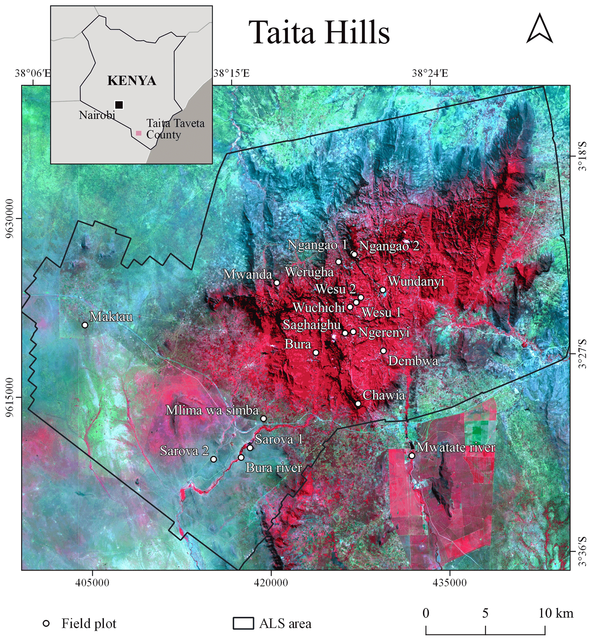
Figure 1Field plots with microclimate sensors in Taita Taveta County, Kenya. ALS refers to airborne laser scanning. The base map is a false color Landsat 8 OLI image from 4 July 2019.
2.2 Airborne laser scanning data
We applied an ALS-based digital elevation model (DEM) raster at 1 m resolution and a CC raster at 30 m resolution. The ALS data for the hills were acquired in February 2014 and February 2015 and the data for lowland areas in March 2014. The mean pulse density of the ALS data in the hills was 3.1 pulses per square meter and mean return density 3.4 returns per square meter, and for the lowlands the pulse density was 1.04 pulses per square meter. The ALS data used in this study are described in detail in Adhikari et al. (2017) and Amara et al. (2020) with the description of pre-processing and derivation of DEM and CC rasters.
We resampled the DEM to 30 m resolution to fit to the spatial resolution of the Landsat 8 image and utilized it to derive the topographic factors of slope degree (∘) and aspect (∘) using ArcGIS Pro spatial analyst tools.
2.3 Microclimatological field measurements
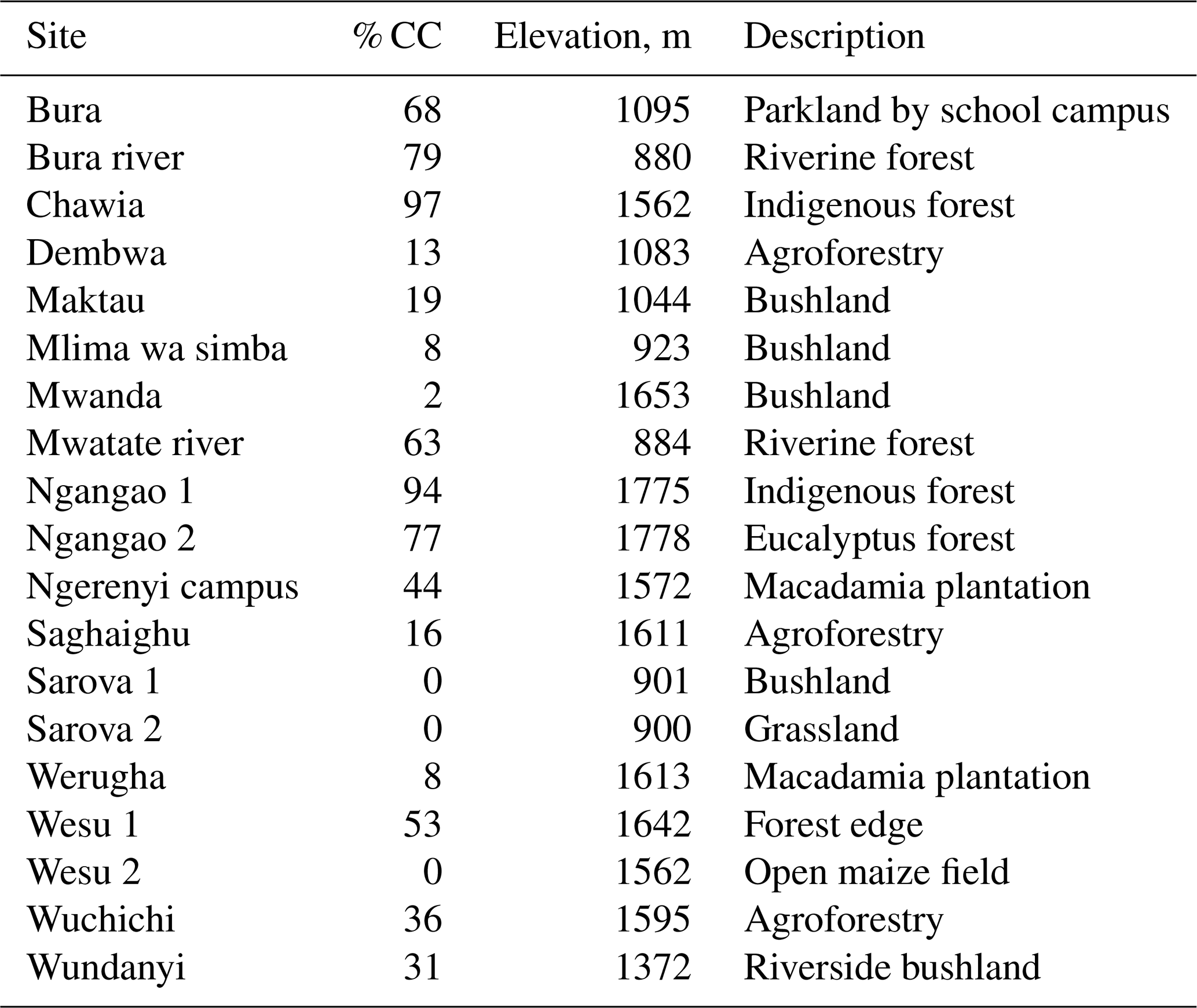
Based on the CC raster derived from the ALS data, we selected a total of 19 field plots representing different CC levels (Table 1). In the plots, we installed TOMST TMS-4 microclimate sensors to measure temperature at three different heights: soil at 6 cm below ground, surface at 2 cm above ground, and air temperature at 15 cm above ground (Tsoil, Tsurface, and Tair, respectively) (Wild et al., 2019). The sensors were deployed in places that were as flat as possible to reduce the effect of slope and that received both sunlight and shade during the day with the changing sun angles. In high CC sites, the sensors were shaded most of the day, while in the open areas, the sensors were exposed to sunlight all day.
The sensors measured parameters every 15 min from 13 to 10 July 2019. We calculated daytime temperature aggregates between sunrise and sunset, local time 06:30–18:30 UTC+3 h (all times are UTC+3 h). We calculated maxima as the mean of daily maxima and minimum temperatures as the mean of minimum temperatures based on the 24 h cycle.
To isolate the influence of CC on microclimate, we quantified and later removed the effect of topography, such as elevation (m) and slope (∘), on temperature. We examined the relationships between the variables first with Pearson's correlation using elevation, slope, and CC as explanatory variables in a multiple regression model. Elevation and CC were the only statistically significant variables. We corrected the daytime mean temperatures according to the altitudinal lapse rates, which were 7.26 ∘C km−1 for soil temperature (Tsoil), 8.09 ∘C km−1 for surface temperature (Tsurface), and 8.06 ∘C km−1 for air temperature (Tair). In the case of diurnal analysis, we applied separate lapse rates for each hour that were derived from the regression analyses. The lapse rates were 6.1–8.2 ∘C km−1 in Tsoil, 3.8–10.4 ∘C km−1 in Tsurface, and 3.3–10.2 ∘C km−1 in Tair. To find the relationships between temperature, CC, and topographic variables, we conducted statistical analyses, including descriptive statistics, linear regression, and Pearson's correlation. We used standard deviation (SD) to describe the variability of temperatures. We used RStudio (R Core Team, 2019) for all statistical analyses.
The ALS data was 4–5 years older than the field measurements. Moreover, the ALS data were collected during the short dry season, in contrast to the field measurements, which we carried out during the start of the long dry season in June 2019. To address the mismatch between the data collection dates, we acquired hemispherical photography at each field plot for validating the CC raster. The differences in CC were not statistically significant, and we considered the estimates consistent enough for proceeding with the analysis using CC from ALS. In the case of Mwatate river plot, CC was retrieved by hemispherical photography only because the plot was outside of the ALS coverage. The methodology is described in Appendix A.
Table 1Names, canopy cover (CC) percentages, elevations, and descriptions of field plot sites.
2.4 Land surface temperature
To observe the effect of CC on temperature in Taita Taveta County, we applied Landsat 8 Operational Land Imager (OLI) thermal infrared sensor (TIRS) satellite image data, downloaded from USGS Earth Explorer (https://earthexplorer.usgs.gov/, last access: 19 July 2019). The bands 10 and 11 of TIRS provide thermal infrared imagery at a resolution of 100 m, but we resampled the band to 30 m to be in concert with the OLI images. The image used in the study was a Level-1 scene obtained on 4 July 2019 at approximately 10:30 UTC+3 h with solar azimuth angle of 45.6∘ and solar elevation angle of 52.1∘. The cloud cover of the whole scene was 11.67 %; there was no completely cloudless scene over the study area for the timing of the field measurements.
Several methods have been developed to retrieve LST from Landsat 8. Unfortunately, shortly after the launch of Landsat 8 in 2013, a stray light problem was detected with TIRS band 11, and it was not recommended by USGS to apply it for scientific purposes (USGS, 2017). We applied the workflow by Ndossi and Avdan (2016) and used the single-channel (SC) method by Jiménez-Muñoz and Sobrino (2003) to calculate LST because the SC method needs only one thermal infrared channel and land surface emissivity (LSE) and water vapor content as parameters. Using only one channel may introduce uncertainty in LST estimations: for Landsat 8 band 10, Jiménez-Muñoz et al. (2014) reported RMSE = 1.5 K, while in Ndossi and Avdan (2016) the RMSE = 3.06 ∘C. Nevertheless, the SC method is most accurate for sensors with effective wavelengths near to 11 µm (Jiménez-Muñoz et al., 2014), the wavelength of Landsat 8 band 10 being 10.6–11.19 µm.
We calculated LSE using the algorithm based on the NDVI image, where pixels were given pre-defined emissivity values based on the NDVI derived from the red, green, and infrared bands. Please refer to Ndossi and Avdan (2016) for more details. Water vapor content at the time of the satellite overpass was 1.7 g cm−2 and was calculated with Eq. (1) using the relative humidity and temperature data obtained from the local weather station:
where w is water vapor content, T0 is air temperature, and RH is relative humidity.
The SC formula is shown in Eq. (2):
where Ts is LST, γ is a parameter depending on Eq. (3), δ is a parameter depending on Eq. (4), ε is land surface emissivity, Lsen is top of atmosphere spectral radiance (W sr−1 m−2 µm−1), bγ = 1324 K for Landsat 8 band 10, and Tsen is sensor brightness temperature (K). We obtained the atmospheric parameters Ψ1, Ψ2, and Ψ3 with Eq. (5).
According to Jiménez-Muñoz, et al. (2014), the coefficients for atmospheric parameters for Landsat 8 TIRS are as in Eq. (6).
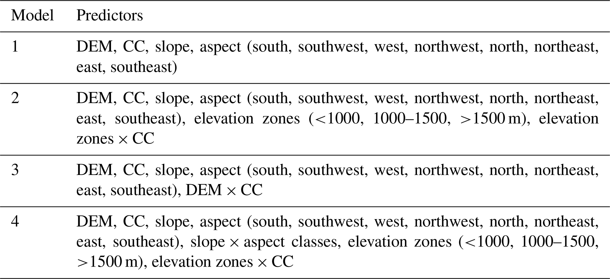
We conducted similar topographic correction with the Landsat image as with microclimate sensors to exclude the effect of topography on LST. Topographic variables (elevation, slope, and aspect), CC, and their interaction terms were included as independent factors and LST as the dependent factor in four multiple regression models (Table 2). We classified aspect to nine classes indicating eight cardinal directions (south, southwest, west, northwest, north, northeast, east, southeast) and flat surface. The classes were treated as dummy variables due to their categorical nature. We also classified elevation to three classes: below 1000, 1000–1500, and above 1500 m. We used the LST at an elevation of 880 m, slope of 0∘, and aspect class north as reference.
Table 2Topographic and canopy cover (CC) predictors included in the four multiple regression models used in the analysis of Landsat 8 land surface temperature.
3.1 Canopy cover and microclimate
3.1.1 Mean, maximum, and minimum temperatures
Topographically corrected mean temperatures (T′) had significant negative correlation with CC at all the measurement heights ( and , ). Based on the linear regression, an increase from 0 % to 100 % CC decreased by 5.2 ∘C (R2=0.6), by 5.9 ∘C (R2=0.71), and by 4.6 ∘C (R2=0.71) (Fig. 2). The average effect on combined , , and was 5.2 ∘C (R2=0.68). and were in general higher than .
CC also affected the variability of mean temperatures: SD of temperatures decreased by approximately 0.1 per 10 % CC increase at all measurement heights (Fig. 2). In , the relationship was not as evident as in and : SD decreased distinctly first when the percent of CC was higher than 60 %.
CC had a strong effect on maximum temperatures at all measurement heights, being affected the most. High CC sites experienced the lowest and maxima, while and were the hottest in Maktau and sites with 0 % CC. Here, topographically corrected average maximum temperatures ranged between 30 and 38.5 ∘C. Again, and were generally higher than . The linear models showed that the increase from 0 % CC to 100 % CC decreased the maximum by 9 ∘C (R2=0.69), by 12.1 ∘C (R2=0.74), and by 9.6 ∘C (R2=0.69) (Fig. 3). On average, the difference was 10.2 ∘C. Similarly to mean temperatures, SD of maximum temperatures decreased with increasing CC: showed a more gradual decrease than and , in which SD decreased substantially only in high CC sites (Fig. 3). The SDs of maximum temperatures were higher than those of mean temperatures.
Based on the regression coefficients, which indicate the magnitude of the influence of CC on temperature, the cooling effect of CC was stronger on maximum temperatures than mean temperature. Additionally, whereas CC affected mean more than mean , in maximum temperatures the situation was the opposite, and was more affected by CC than (Figs. 2 and 3).
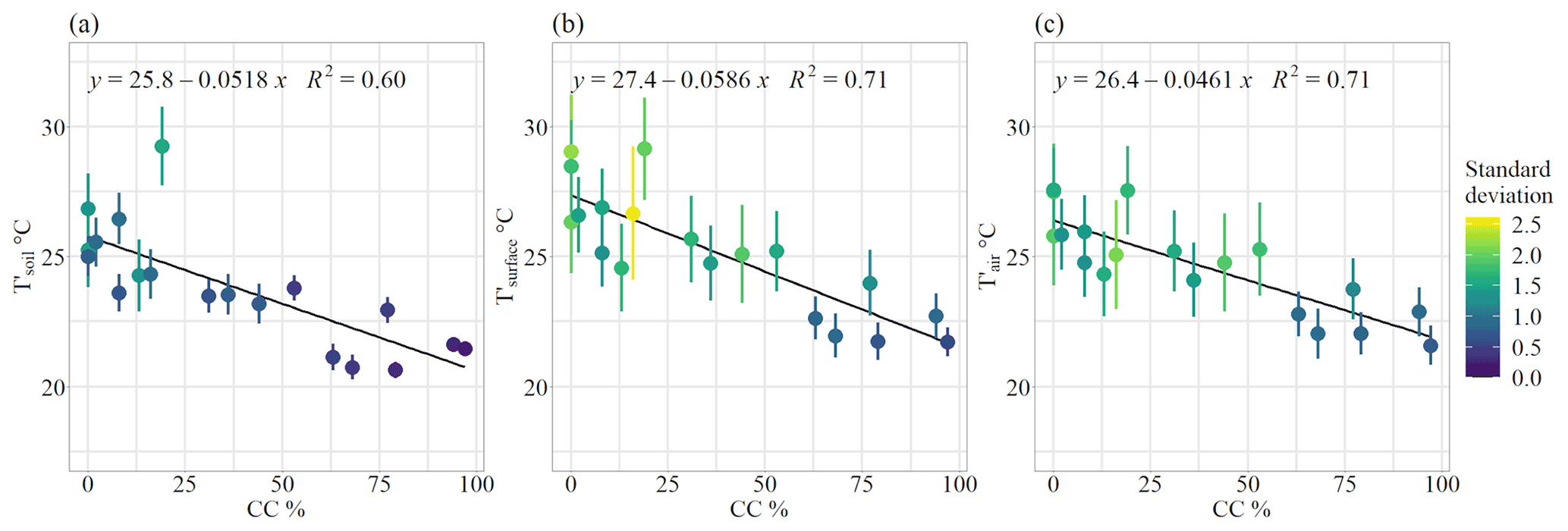
Figure 2Scatterplots of topographically corrected daytime mean temperatures (T′) and standard deviation against canopy cover (CC) percentage with regression line. (a) Soil temperature. (b) Surface temperature. (c) Air temperature.

Figure 3Scatterplots of topographically corrected daytime maximum temperatures (T′) and standard deviation against canopy cover (CC) percentage with regression line. (a) Soil temperature. (b) Surface temperature. (c) Air temperature.
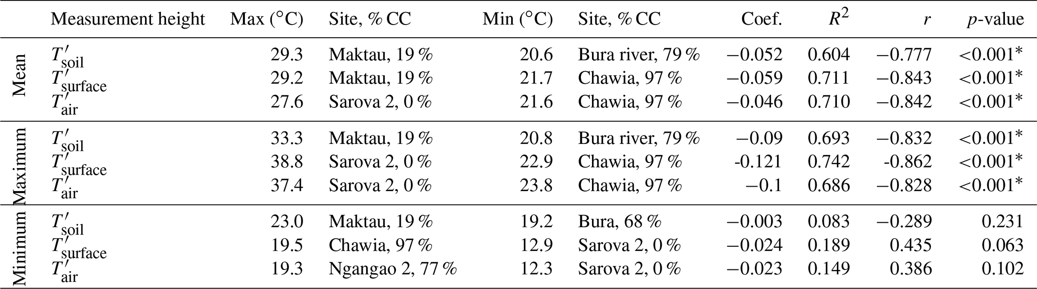
Minimum temperatures showed no explicit relationship with CC, and sites with similar CC had high temperature variability. R2 were low (<0.2) at all measurement heights, and correlations between temperatures and CC were insignificant. All results from the regression analyses are summarized in Table 3.
Table 3Topographically corrected temperature (T′) statistics for the soil, surface, and air. Temperatures in the maximum and minimum columns refer to the highest and lowest mean, maximum, and minimum temperatures. Site refers to where the highest and lowest temperatures were measured and their respective canopy cover (CC) percentage. * Indicates statistical significance.
3.1.2 Temporal variation
Figure 4 presents the daily variation in topographically corrected daytime mean temperatures. The effect of CC was evident at all three measurement heights: mean temperatures were lower in high CC sites than in open areas, yet some low CC sites exhibited relatively low temperatures. For example, on July 2, which was one of the hottest days of the study period, temperature differences between the hottest (Maktau, 19 % CC) and coolest (Ngangao 1, 94 % CC) sites were 11.0 ∘C in , 11.3 ∘C in , and 9.8 ∘C in . Even during the coldest days, temperatures were lower in sites with dense canopies than in open land. Especially in the sites with high CC remained relatively stable from day to day, showing little fluctuation even during the hot day streaks: differences in mean temperatures remained even less than 1 ∘C between the hottest and coolest days.
The cooling effect of CC varied throughout the study period: on hot days, the cooling effect (described by CC's regression coefficient in Fig. 4) increased, while on cooler days, the cooling effect decreased. The strongest cooling took place in on June 23, when CC's cooling effect was 7.6 ∘C. had overall the highest cooling effect (3.3–7.6 ∘C) and the weakest (2.6 ∘C). In , the cooling effect was 3.2–6.9 ∘C (Fig. 4).
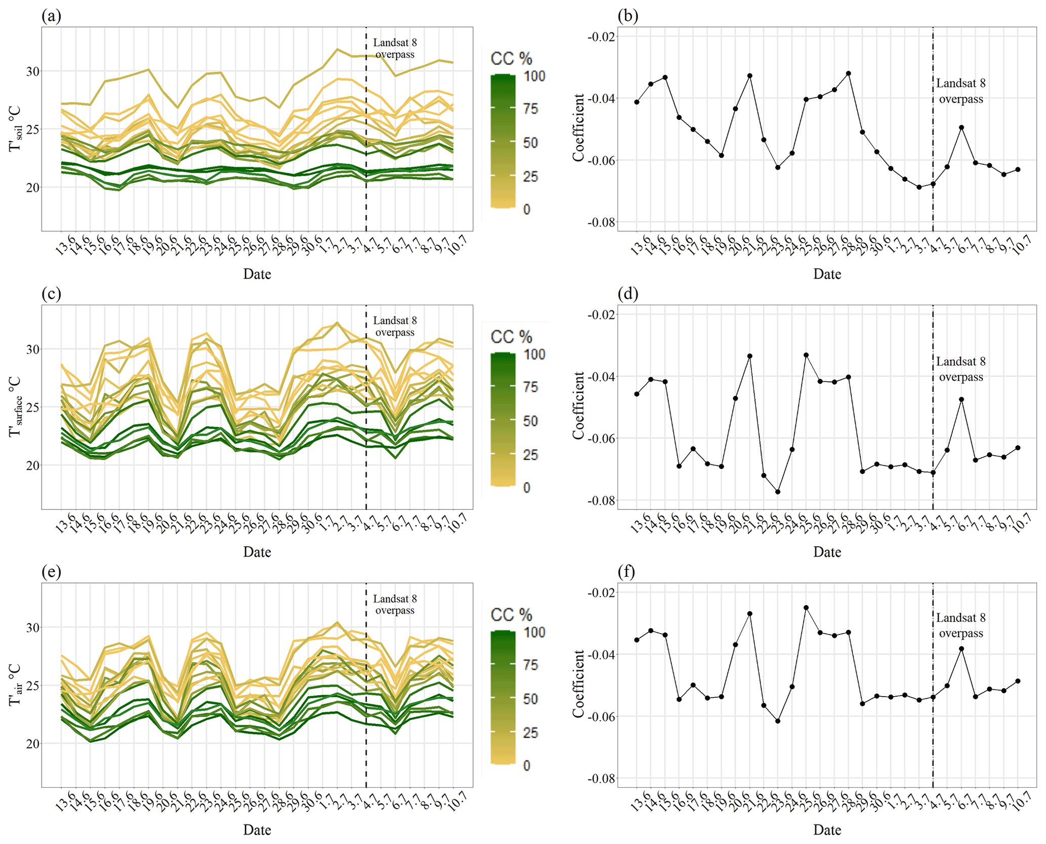
Figure 4Daily variation in topographically corrected daytime (6.30–18.30) mean temperatures (T′) between 13 June and 10 July 2019 (a, c, e) and cooling effect of canopy cover (described by regression coefficient) (b, d, f). Line color indicates canopy cover (CC) percentage. Dashed line represents the overpass date of Landsat 8 (4 July 2019). (a–b) Soil temperature. (c–d) Surface temperature. (e–f) Air temperature.
Figure 5 shows the intra-daily temperature variability based on study period means. was more stable than and , which showed higher peaks and drops. In the morning, temperatures at all measurement heights started to rise rapidly between 06:00 and 08:00. Changes in seemed to lag a couple of hours behind and : they reached the highest readings between 11:00 and 15:00, while peaked between 15:00 and 17:00. Further, after peaking, temperatures decreased before stabilizing between 19:00 and 20:00 in and , while decreased slower. Tsoil remained warmer during the night than the other two measurement heights.
Figure 5 also describes the correlation between CC and temperatures. The impact of CC was the lowest in the morning, when the temperatures also reached their minima. The strongest correlation (r<−0.8) occurred during the afternoon at all measurement heights. correlated negatively with CC throughout the day, in contrast to and , whose correlations were positive during the night.
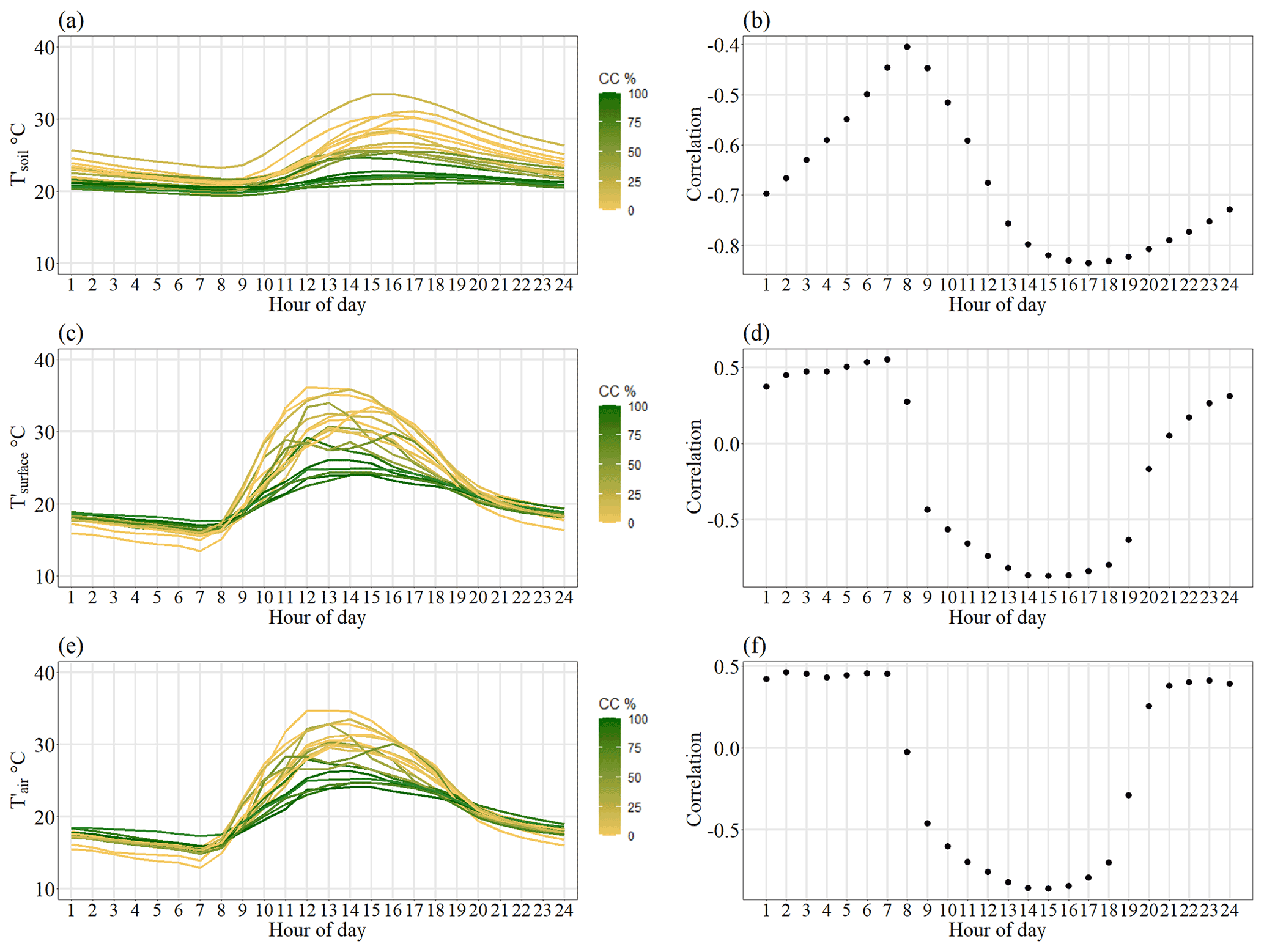
Figure 5Topographically corrected diurnal mean temperatures (T′) (a, c, e) and the correlation between T′ and canopy cover (CC) percentage (b, d, f) between 13 June and 10 July 2019. Hour refers to ordinal number of hour, e.g., 1 means 00:00–01:00. Line color indicates CC percentage. (a–b) Soil temperature. (c–d) Surface temperature. (e–f) Air temperature.
3.2 Landsat 8 land surface temperature
3.2.1 Land surface temperature compared with temperatures measured in the field
LST and raw field temperatures (T) at the time of satellite overpass showed statistically significant correlation (r=0.82, 0.79, and 0.84 at Tsoil, Tsurface, and Tair, respectively) (Fig. 6). At 18 sites out of 19, LST was higher than Tsoil, whereas between LST and Tsurface or Tair there was no consistent difference. Mean differences were 4.1 ∘C (Tsoil), −0.03 ∘C (Tsurface), and 0.57 ∘C (Tair). The Tsoil difference was statistically significant with 95 % confidence, while Tsurface and Tair differences were not.
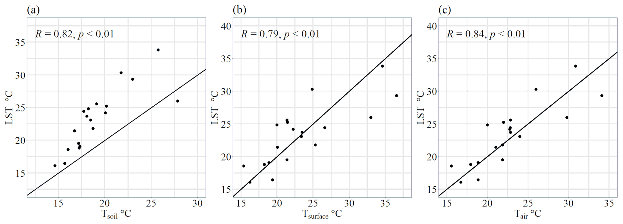
Figure 6Landsat 8 land surface temperature (LST) compared with raw field temperatures (T) at the time of satellite overpass (10:30) on 4 July 2019. (a) LST and soil temperature. (b) LST and surface temperature. (c) LST and air temperature.
3.2.2 Impact of canopy cover and topography on land surface temperature
Topographic variables elevation, slope, and aspect all had a significant effect on LST. In all four models, the elevational lapse rates varied from 11 to 15 ∘C km−1. Aspect, in turn, had a varying impact depending on the model, but the general trend was that south, southwest, and west had the highest cooling, as was expected at the time of the day. The effect of slope decreased as the models became more complex, and the joint impacts of slope and aspect in Model 4 were greater than the effects of slope or aspect alone. The results of all four models can be found in Appendix B.
All the variables in Model 1 showed statistical significance (R2=0.74). Based on the regression analysis, generally the increase from 0 % CC to 100 % CC decreased LST by 5 ∘C. After the exclusion of other variables except CC, correlation between LST and CC was −0.37 (p<0.001) and R2=0.14.
In Model 2, three elevation zones (below 1000, 1000–1500, above 1500 m) were added to the model. This increased the R2 to 0.77, demonstrating a notable difference in the cooling effect of CC depending on elevation zone. At the elevations below 1000 m, the cooling effect of CC when moving from 0 % CC to 100 % CC was 6.8 ∘C, between 1000–1500 m the effect was 3.7 ∘C, and above 1500 m the effect was 4 ∘C. Roughly, the cooling impact of CC above 1000 m decreased to almost half of the impact in the lowlands.
In Model 3, the interaction term of CC and elevation zones was replaced with the interaction term of CC and the continuous variable elevation from the DEM. This produced R2=0.74. The coefficient for the interaction term was 0.00005, indicating that an increase of 1000 m in elevation decreased the cooling effect of CC by 0.05 ∘C. The model performed poorer compared to Model 2.
Model 4 was built up on Model 2 by adding interaction terms between slope and aspect classes. Model 4 performed the best of the four (R2=0.77), but the difference was not large compared to Model 2. The cooling effect of CC in the lowlands was 6.8 ∘C, the same as in Model 2. In the 1000–1500 m elevation zone the cooling effect was 3.7 ∘C, and above 1500 m it was 3 ∘C. The cooling effect of CC in the 1000–1500 m zone had the same magnitude as in Model 2, and it decreased by a further 0.7 ∘C at elevations above 1500 m.
In summary, including either of the elevation factors (DEM or elevation zones) in the model showed that elevation affected CC's cooling effect significantly, having an almost 2 times higher impact in the lowlands compared to the hills. The dependence of CC's impact on elevation is demonstrated in Fig. 7 using eight elevation classes. CC's regression coefficients decreased with increasing elevation after 1000 m, yet increased again between 1200 and 1400 m to roughly the same as in the lowlands. The effect was the smallest at elevations above 1800 m.
Figure 7Density plots of topographically corrected land surface temperature (LST′) and canopy cover (CC) percentage in eight elevation classes with regression line. (a) Below 800 m. (b) 800–1000 m. (c) 1000–1200 m. (d) 1200–1400 m. (e) 1400–1600 m. (f) 1600–1800 m. (g) 1800–2000 m. (h) Above 2000 m.
High CC decreased near-ground mean temperatures on average by 5.2 ∘C compared to open land, depending on measurement height. The difference was even greater in temperature maxima, which has been reported to be the case also by De Frenne et al. (2019) and Belsky et al. (1989). Temperature and CC had a linear relationship, pointing out that closed CC was not needed for a substantial cooling effect.
Tsurface was affected the most by CC. Despite the measurement height of Tsurface being only 13 cm below Tair, the effect of CC was notably weaker in Tair, which is in line with previous studies. For example, Davis et al. (2019) report that the effect of CC was weaker at 2 m than at 10 cm height, while in De Frenne et al. (2019) temperature offset between forest and open land was the greatest close to the ground. In Belsky et al. (1989), soil temperature was the least affected by CC. Luyssaert et al. (2014) compared air temperature and LST and report that the temperature of the planetary boundary was less affected than LST by the removal of forest cover.
Macroclimate affected the magnitude of the cooling: based on the temporal data from the microclimate sensors, during the cooler days of overcast conditions, CC's cooling effect was smaller. Additionally, the temperature differences between low and high CC sites were smaller during these days. In the case of LST, elevation impacted the cooling effect: above 1000 m, the cooling effect decreased by approximately 50 % to that of the lowlands. It can be concluded that trees' importance in controlling temperatures increases in hotter environments. The finding is meaningful because agricultural expansion at the cost of woody vegetation cover in the area is predicted to take place predominantly in the lowlands (Erdogan et al., 2011; Maeda et al., 2010), where the temperatures are very high. Increasing tree cover on farmlands could thus be of considerable benefit in decreasing local temperatures.
Our finding is in parallel with findings by Zeng et al. (2021), who reported an elevational effect of deforestation on temperatures in the Albertine Rift Mountains: the warming effect of deforestation decreased with elevation and disappeared at elevations above 3000 m. This phenomenon resembles the latitude-dependent effect of forests on temperatures: in tropical areas, there is more cooling, while boreal forests cause more warming (Lee et al., 2011; Li et al., 2015). Plant evapotranspiration rates are relative to the solar radiation, ambient temperatures, and water balance (Geiger, 1980; Allen et al., 1998; Davis et al., 2019), decreasing the demand for evapotranspiration at low temperatures caused by elevational lapse rate or cool weather conditions. During clear weather, canopies absorb and reflect most of the incoming solar radiation creating cooler conditions in the understory, together with evapotranspiration, whereas cloud cover causes a total reduction in the incoming short-wave radiation (Geiger, 1980; De Frenne et al., 2021). Moreover, while the evapotranspirative cooling mostly offsets warming caused by canopy albedo, at high elevations the albedo effect stays constant, and evapotranspiration decreases (Zeng et al., 2021).
The impact of CC on microclimate was different on different days and is likely to vary during different times of the year (Davis et al., 2019; De Frenne et al., 2021). We expect this to be the case with LST as well. For instance, Maeda and Hurskainen (2014) found that land cover's influence on LST at Mount Kilimanjaro varied seasonally and diurnally, and the effect was dependent on elevation. Our LST estimation was only a snapshot for 4 July 2019, a sunny, almost cloud-free day, and does not represent the year-round situation experiencing two rainy seasons, which are cloudy. In the hills, cloudy and misty conditions are experienced throughout the year (Helle, 2016; Räsänen et al., 2018). A time series comparing the cooling effect of CC over seasons and several years is an interesting future research topic, as the TOMST sensors remained in the 19 field plots. It would be interesting to model the sunshine hours every day in the locations of the TOMST sensors using the hemispherical photography in order to assess how many hours of the day the tree cover causes shadows over the sensor.
Canopies control the thermal environments of forests to a high extent (De Frenne et al., 2019; Davis et al., 2019), which was reaffirmed in this study. Therefore, CC can mitigate large-scale macroclimate warming (De Frenne et al., 2019). An increase of 2 ∘C of the global temperature as a consequence of enhanced greenhouse effect can have detrimental impacts on the most vulnerable ecosystems (IPCC, 2018). Because the time span of local changes in temperatures due to LULCC is much shorter than in the global climate change, the regional and local consequences can be of even higher magnitude (Potter et al., 2013; Chen et al., 1999). Due to the debts of species' adaptation capabilities to climate warming (Zellweger et al., 2020), changes in the microclimate temperatures may be fatal for flora and fauna occupying narrow thermal niches. This may further impact biodiversity and consequently the crucial ecosystem services provided by forests that take place close to ground surface (Chen et al., 1999; Zellweger et al., 2020).
Forest fragmentation decreases the ability of tropical forests to mitigate climate change (Ewers and Banks-Leite, 2013), but on regional scale even small forests have an impact on LST (Mildrexler et al., 2011). Our results from the linear models revealed that TOF had the same effect on local temperatures as forests despite the smaller magnitude and could hence help in conserving biodiversity. For instance, Mendenhall et al. (2016) found that in Costa Rica farm trees increased the number of tree and plant species. Most of the CC in Taita Hills comprises TOF occurring on farms and in human settlements. Sites with agroforestry trees and moderate CC were already experiencing both lower mean and maximum temperatures than the open sites.
The importance of TOF is receiving more attention (Kuyah et al., 2019; Skole et al., 2021), and in Taita Hills, Pellikka et al. (2018) reported an addition in carbon stocks since 2003. The agriculture rules (Agriculture (Farm Forestry) Rules, 2009) of 2009 requires that at least 10 % forest cover should be left or planted on farms. Based on our results, this 10 % CC makes a significant difference in temperatures (−0.5 ∘C in mean and −1 ∘C in maximum temperatures; −0.5 ∘C in LST). Soil and air temperatures impact crop productivity, and furthermore, the fog deposit captured by trees brings more water to plants. In general, increasing temperatures make plant growth more efficient, but this is the case only as long as the increase occurs within the thermal limits of the plant's tolerance (Muimba-Kankolongo, 2018). As extreme heat and precipitation events are becoming more common with climate change (MoALF, 2016; IPCC, 2018), the negative effects of warming will become notable in sub-Saharan Africa. This further threatens the food security and especially the most common crop, maize, which is one of the most vulnerable crops in terms of climate change in Africa (Cairns et al., 2013; Adhikari et al., 2015). Forests of Taita Hills contribute to the food security by capturing atmospheric moisture as fog deposit and storing the water, providing water for farms in the foothills and lowlands (Pellikka et al., 2013; Helle, 2016). In addition to dew capture, agroforestry has been shown to contribute to improved soil moisture (Rhoades, 1995; Siriri et al., 2013), hydraulic conductivity (Nyamadzawo et al., 2003, 2007), and water storage (Makumba et al., 2006; Nyamadzawo et al., 2012).
The pressure on tropical forests in sub-Saharan Africa is caused by many factors, fuelwood collection being significant (Abdelgalil, 2004; Zschauer, 2012), which could be mitigated by increasing the tree cover on farms (Unruh et al., 1993; Ilyama et al., 2014; Chakravarty et al., 2019). The results of this study further encourage an increase in tree cover, particularly in the lowland farms, as a strong potential way to fight the negative effects of climate change. Nevertheless, water is scarce especially in the lowland areas, and trees' vast need for water must be taken into account. The phenomenon is paradoxical because trees improve the water cycle, in general, but consume high amounts of water (Ong et al., 2006). Water balance also affects the temperature buffering capacity of trees (Davis et al., 2019). In areas with water scarcity, the competition for water resources between crops, animals, and people may be a limiting factor in the adoption of agroforestry practices. One solution in the hot lowlands is dew collection, but it would require a tree cover or other surfaces to capture the humidity. In Tuure et al. (2019), artificial surfaces produced at best 0.1 L d−1 of water from morning dew and 25 L in a year.
This study was limited to a short time span and a small sample size in microclimate study sites, which makes it susceptible to uncertainties associated with temporal and spatial variability. Topographic correction was applied on the microclimate data and was calculated based on elevation only. The small amount of observations did not allow for calculating the impact of the aspect, which is expected to exist based on the LST analysis. Due to accounting for the effect of topography, both microclimate and LST estimates did not represent the true values recorded but made the temperatures comparable by CC.
In terms of LST, as has been documented in several studies, spaceborne thermal infrared (TIR) remains an uncertain method for accurate LST retrieval (Simó et al., 2018; Li et al., 2013). After all, LST is an indirect measurement and the results of complicated mathematical processing requiring knowledge of several components, in which error in any of them causes inaccuracies in LST (Simó et al., 2018). We calculated LST using the SC method by Jiménez-Muñoz and Sobrino (2004) due to the stray light problem in Landsat 8 TIRS band 11. While using only one thermal channel for the estimation of LST exposes a high possibility of inaccuracy, band 10 is more suitable for the SC method than band 11 because of higher atmospheric transmissivity (Jiménez-Muñoz et al., 2014). The main sources of error in SC are estimation of atmospheric water vapor content and LSE. LSE is determinant in the correct LST retrieval, yet it is highly difficult to measure and prone to error. Water vapor, in turn, can be highly spatially variable and should be retrieved preferably from satellite data rather than pointwise weather station data (Ndossi and Avdan, 2016). Jiménez-Muñoz et al. (2014) report that water vapor content higher than 3 g cm−2 causes unacceptable inaccuracy: in this study, the water vapor content was 1.7 g cm−2, which decreases the possible error. Wang et al. (2019) conclude that the SC is a valid method for Landsat 8 processing and produces results with an accuracy that is high enough for most purposes; Ndossi and Avdan (2016) found that SC was the second best algorithm for the retrieval of Landsat 8 LST. SC has been applied successfully also by, for example, He et al. (2019). Moreover, in dense canopies the signal constitutes mostly the upper canopy (Bense et al., 2016; Zellweger et al., 2019), and previous studies have not so far demonstrated LST's relationship with understory conditions. We showed how LST provided consistent results particularly with Tsurface and Tair. Therefore, this study contributed to clarifying the relationship of the upper canopy and the understory.
Our study provided information about a topic whose importance has only recently been recognized (De Frenne et al., 2013; Jucker et al., 2018; Davis et al., 2019; Zellweger et al., 2020). Research and modeling of climate change implications on microclimate cannot rely on observations from weather stations with low spatial resolution but need data that represent the microclimatic conditions relevant for most ecosystem functions (Potter et al., 2013). Previous research about vegetation and LST has been often conducted at much lower spatial resolutions and applied less accurate topographic correction (Li et al., 2015). Furthermore, the effect of trees on climate is usually studied solely based on comparison between forest and open land (De Frenne et al., 2019), neglecting the intermediate canopies and their significance, despite the fact that human activity is focused mostly in areas with TOF. We used microclimate data covering a CC gradient and satellite-derived LST data combined with a DEM of 30 m acquired with ALS over the versatile study area. While establishing field observation networks with wide spatial coverage remains a challenge, our results showed that LST can be used as a proxy for assessing the impacts of CC on microclimate.
Future research should further investigate the contribution of varied factors to microclimate. For example, since all trees are not of equal benefits in agroforestry, more studies could be targeted at the comparison of different agroforestry species' cooling potential, as well as the potential of plantation forests. Including soil moisture, air temperature, and comprehensive field plot networks under different canopy structures in the future analyses should broaden the knowledge about trees' role in mitigating and adapting to climate change.
Our results demonstrate a consistent but heterogeneous influence of canopy cover on the microclimate of highly diverse tropical ecosystems. Daytime temperatures correlated inversely with canopy cover, the effect being strongest on surface temperatures. In hotter environments, the difference between sites of high and low canopy cover became most notable. The cooling effect did not exist only with high canopy cover, but even intermediate canopy cover and trees outside forest buffered the hottest temperatures. Our results thus provide robust evidence that any efforts in the direction of preserving, restoring, or increasing vegetation cover can have a substantial impact in creating more stable and cooler microclimates. Satellite-based land surface temperature was a suitable proxy for assessing microclimatic variables like surface and near-ground temperatures, particularly in heterogeneous regions where the network of field measurements cannot cover the spatial microclimate variability.
This study provided valuable information about the potential of trees in climate change adaptation and mitigation in tropical environments. As the effect of canopy cover on microclimate increased at lower elevations and during hot days, our results indicate that warmer and drier regions are likely to benefit the most from trees.
We took hemispherical photographs at every microclimate sensor site. The camera in use was a Nikon D5000 SLR and the lens a Sigma 4.5 mm F2.8 EX DC HSM Circular Fisheye. The camera was attached to a tripod during the taking of photographs. We took photographs at two different heights: the lowest possible tripod adjustment to be as close to the actual sensor level as possible, which was around 60 cm, and at eye level around 130 cm. We took photographs at eye level also from every intercardinal direction 15 m away from the sensor. The camera was adjusted looking upward with the top of the camera pointing north. Two images at every height and direction were taken with different settings: first image on program mode with automatic aperture and shutter speed and the second on manual mode with the rest of the settings staying the same as in picture one, except shutter speed was reduced to half of the first image. The ISO value was set as constant at 500. The purpose of the lower shutter speed was to reduce the impact of light conditions that were not optimal, meaning direct sunlight that causes overexposure of images which in turn makes them difficult to analyze. Optimally, the photographs should be taken under constant cloud cover or at dawn or dusk (Pellikka et al., 2000); however due to the timetable, waiting for better light conditions at some sites was not possible, and thus some images were overexposed.

Figure A1Comparison of canopy cover (CC) percentage retrieved from airborne laser scanning (ALS) and hemispherical photography (HP) with line of identity.
We analyzed the hemispherical photographs in the software Hemisfer (WSL; version 2.2) (Schleppi et al., 2007; Thimonier et al., 2010). From the two images, we used the less exposed one in the analysis. For the calculation of canopy cover, we used the images taken from eye level because they were more comparable to the ALS-based canopy cover, and the photographs from cardinal directions were all taken at eye level. We classified the image pixels to sky and canopy by determining a threshold value to separate dark and light pixels in the image. For most images, we used the automatic threshold method by Nobis and Hunziker (2005). In the case of some images, the algorithm clearly produced errors due to overexposure and direct sunlight; therefore the algorithm by Ridler and Calvart (1978) was applied, or a manual threshold was determined. We used only the blue band in the analysis, apart from photographs in which the classification was failing, and using all the bands produced the best result (Heiskanen et al., 2015a). The gamma correction was γ=2.2. Only the zenith angle range of 0–15∘ was analyzed because errors in canopy cover accuracy increase with larger angles (Paletto and Tosi, 2009). We computed canopy cover by calculating an average of one gap fraction of the five measurements, and this gave a plot-wise canopy cover (Heiskanen, et al., 2015b). Finally, we compared the canopy cover retrieved from hemispherical photography and ALS using Pearson's correlation and Student's t test. The mean of differences was 0.89 and was not statistically significant.
Table B1Summary of regression coefficients in the analysis of land surface temperature (LST) from the four models tested. * Indicates statistical significance.
The data and scripts presented in this study are available on request from the author (Iris J. Aalto).
IJA, EEM, JH, and PKEP conceptualized the research. IJA collected the data, did the investigation, and wrote the paper. PKEP was responsible for funding acquisition. All authors designed the methodology. IJA and EKA performed the formal analysis. EEM and PKEP were responsible for project administration. IJA did the validation. EEM, JH, and PKEP provided supervision. IJA visualized the data. IJA, EEM, JH, and PKEP reviewed and edited the manuscript.
The contact author has declared that none of the authors has any competing interests.
Publisher's note: Copernicus Publications remains neutral with regard to jurisdictional claims in published maps and institutional affiliations.
We would like to acknowledge Agnes Mwangombe, Ali Ndizi, Clemece Mwamburis, Constance Nyatta, Cathrine Mwakesi, Simon Brazil, Moses Onyimbo, and Dalmas Moka secondary school, Jason Collette and Teita Sisal Estate, St. Mary's Teachers' Training College, and Taita Taveta University Ngerenyi campus for allowing us to conduct this research on their properties. We also thank Taita Research Station of the University of Helsinki for logistical support during the field work campaign. Special thanks to Mwadime Mjomba for assistance during the field work. We acknowledge Matti Räsänen for the provision of weather station data and Hari Adhikari for the canopy cover data. We also want to thank the two anonymous reviewers for their comments and suggestions to improve the manuscript.
This study was conducted as part of Smartland project (Environmental sensing
of ecosystem services for developing a climate-smart landscape framework to
improve food security in East Africa, decision no. 31864), funded by the Academy
of Finland, and ESSA project (Earth observation and environmental sensing
for climate-smart sustainable agropastoral ecosystem transformation in East
Africa), funded by the European Commission DG International Partnerships DeSIRA
program (FOOD/2020/418-132). Eduardo Maeda was funded by the Academy of
Finland (decision numbers 318252 and 319905).
Open-access funding was provided by the Helsinki University Library.
This paper was edited by Christopher Still and reviewed by two anonymous referees.
Abdelgalil, E. A.: Deforestation in the drylands of Africa: Quantitative modelling approach, Environ. Dev. Sustain., 6, 415–427, https://doi.org/10.1007/s10668-005-0787-1, 2004.
Abera, T. A., Heiskanen, J., Pellikka, P. K., Adhikari, H., and Maeda, E. E.: Climatic impacts of bushland to cropland conversion in Eastern Africa, Sci. Total. Environ., 717, 137255, https://doi.org/10.1016/j.scitotenv.2020.137255, 2020.
Adhikari, H., Heiskanen, J., Siljander, M., Maeda, E., Heikinheimo, V., and Pellikka, P. K.: Determinants of Aboveground Biomass across an Afromontane Landscape Mosaic in Kenya, Remote Sens., 9, 827, https://doi.org/10.3390/rs9080827, 2017.
Adhikari, U., Nejadhashemi, A. P., and Woznicki, S. A.: Climate change and eastern Africa: a review of impact on major crops, Food Energ. Secur., 4, 110–132, https://doi.org/10.1002/fes3.61, 2015.
Allen, R. G., Pereira, L. S., Raes, D., and Smith, M.: Crop Evapotranspiration – Guidelines for Computing Crop Water Requirements, FAO Irrigation and Drainage Paper 56, United Nations Food and Agriculture Organization, Rome, ISBN 92-5-104219-5 1998.
Amara, E., Adhikari, H., Heiskanen, J., Siljander, M., Munyao, M., Omondi, P., and Pellikka, P.: Aboveground Biomass Distribution in a Multi-Use Savannah Landscape in Southeastern Kenya: Impact of Land Use and Fences, Land, 9, 381, https://doi.org/10.3390/land9100381, 2020.
Beer, C., Reichstein, M., Tomelleri, E., Ciais, P., Jung, P., Carvalhais, N., Rödenbeck, C., Arain, M. A., Baldocchi, D., Bonan, G. B., Bondeau, A., Cescatti, A., Lasslop, G., Lindroth, A., Lomas, M., Luyssaert, S., Margolis, H., Oleson, K. W., Roupsard, O., Veenendaal, E., Viovy, N., Williams, C., Woodward, F. I., and Papale, D.: Terrestrial Gross Carbon Dioxide Uptake Distribution and Covariation with Climate, Science, 329, 834–838, https://doi.org/10.1126/science.1184984, 2010.
Belsky, A. J., Amundson, R. G., Duxbury, J. M., Riha, S. J., Ali, A. R., and Mwonga, S. M.: The Effects of Trees on Their Physical, Chemical and Biological Environments in a Semi-Arid Savanna in Kenya, J. Appl. Ecol., 26, 1005–1024, https://doi.org/10.2307/2403708, 1989.
Bense, V. F., Read, T., and Verhoef, A.: Using distributed temperature sensing to monitor field scale dynamics of ground surface temperature and related substrate heat flux, Agr. Forest. Meteorol., 220, 207–215, https://doi.org/10.1016/j.agrformet.2016.01.138, 2016.
Cairns, J. E., Hellin, J., Sonder, K., Araus, J. L., MacRoberts, J. F., Thierfelder, C., and Prasanna, B. M.: Adapting maize production to climate change in sub-Saharan Africa, Food Secur., 5, 345–360, https://doi.org/10.1007/s12571-013-0256-x, 2013.
Chakravarty, S., Pala, N. A., Tamang, B., Sarkar, B. C., Abna Manohar K., Rai, P., Puri, A., and Shukla, G.: Ecosystem services of Trees Outside Forest, in: Sustainable Agriculture, Forest and Environmental Management, edited by: Jhariya, M. K., Banerjee, A., Meena, R. S., and Yadav, D. K., Springer, https://doi.org/10.1007/978-981-13-6830-1_10, 2019.
Chen, J., Saunders, S. C., Crow, T. R., and Naiman, R. J.: Microclimate in forest ecosystem and landscape ecology, Bioscience, 49, 288–297, https://doi.org/10.2307/1313612, 1999.
Das, A., Nagendra, H., Anand, M., and Bunyan, M.: Topographic and Bioclimatic Determinants of the Occurrence of Forest and Grassland in Tropical Montane Forest-Grassland Mosaics of the Western Ghats, India, PLoS One, 10, e0130566, https://doi.org/10.1371/journal.pone.0130566, 2015.
Davis, K., T., Dobrowski, S. Z., Holden, Z. A., Higuera, P. E., and Abatzoglou, J. T.: Microclimate buffering in forests of the future: the role of local water balance, Ecography, 42, 1–11, https://doi.org/10.1111/ecog.03836, 2019.
De Frenne, P., Rodríguez-Sánchez, F., Coomes, D. A., Baeten, L., Verstraeten, G., Vellend, M., Bernhardt-Römermann, M., Brown, C. D., Brunet, J., Cornelis, J., Decocq, G. M., Dierschke, H., Eriksson, O., Gilliam, F. S., Hédl, R., Heinken, T., Hermy, M., Hommel, P., Jenkins, M. A., Kelly, D. L., Kirby, K. J., Mitchell, F. J. G., Naaf, T., Newman, M., Peterken, G., Petrik, P., Schultz, J., Sonnier, G., Van Calster, H., Waller, D. M., Walther, G-R., White, P. S, Woods, K. D., Wulf, M., Graae, B. J., and Verheyen, K.: Microclimate moderates plant responses to macroclimate warming, P. Natl. Acad. Sci. USA, 110, 18561–18565, https://doi.org./10.1073/pnas.1311190110, 2013.
De Frenne, P., Zellweger, F., Rodríguez-Sánchez, F., Scheffers, B. R., Hylander, K., Luoto, M., Vellend, M., Verheyen, K., and Lenoir, J.: Global buffering of temperatures under forest canopies, Nat. Ecol. Evol., 3, 744–749, https://doi.org/10.1038/s41559-019-0842-1, 2019.
De Frenne, P., Lenoir, J., Luoto, M., Scheffers, B. R., Zellweger, F., Aalto, J., Ashcroft, M. B., Christiansen, D. M., Decocq, G., De Pauw, K., Govaert, S., Greiser, C., Gril, E., Hampe, A., Jucker, T., Klinges, D. H., Koelemeijer, I. A., Lembrechts, J. J., Marrec, R., Meeussen, C., Ogée, J., Tyystjärvi, V., Vangansbeke, P., and Hylander, K.: Forest microclimates and climate change: Importance, drivers and future research agenda, Glob. Chang Biol., 27, 2279–2297, https://doi.org/10.1111/gcb.15569, 2021.
Ellison, D., Morris, C.E., Locatelli, B., Sheil, D., Cohen, J., Murdiyarso, D., Gutierrez, V., van Noordwijk, M., Creed, I. F., Pokorny, J., Gaveau, D., Spracklen, D. V., Tobella, A. B., Ilstedt, U., Teuling, A. J., Gebrehiwot, S. G., Sands, D. C., Muys, B., Verbist, B., Springgay, E., Sugandi, Y., and Sullivan, C. A.: Trees, forests and water: Cool insights for a hot world, Global Environ. Chang., 43, 51–61, https://doi.org/10.1016/j.gloenvcha.2017.01.002, 2017.
Erdogan, H. E., Pellikka, P. K., and Clark, B.: Modelling the impact of land-cover change on potential soil loss in the Taita Hills, Kenya, between 1987 and 2003 using remote-sensing and geospatial data, Int. J. Remote Sens., 32, 5919–5945, https://doi.org/10.1080/01431161.2010.499379, 2011.
Ewers, R. M. and Banks-Leite, C.: Fragmentation Impairs the Microclimate Buffering Effect of Tropical Forests, PLoS One, 8, e58093, https://doi.org/10.1371/journal.pone.0058093, 2013.
FAO: Global Forest Resources Assessment 2000 (FRA 2000), Food and Agriculture Organization of the United Nations, Rome, Italy, ISBN 978-9251046425, 2000.
FAO: FRA 2015 terms and definitions, Forest Resources Assessment Working Paper 180, Food and Agricultural Organization of the United Nations, Rome, Italy, 2012.
FAO: Global forest resources assessment 2015. How are the world's forests changing?, 2nd Edn., Food and Agriculture Organization of the United Nations, Rome, Italy, ISBN 978-92-5-109283-5, 2016.
Agriculture (Farm Forestry) Rules: Cap. 318 (KEN), https://www.fao.org/faolex/results/details/en/c/LEX-FAOC101360 (last access: 8 April 2021), 2009.
Geiger, R.: The climate near the ground, 4th Edn., Harvard University Press, United States of America, ISBN 978-0674135000, 1980.
Goward, S. N. and Hope, A. S.: Evapotranspiration from combined reflected solar and emitted terrestrial radiation: Preliminary FIFE results from AVHRR data, Adv. Space Res., 9, 239–249, 1989.
Goward, S. N., Cruickshanks, G. D., and Hope, A. S.: Observed relation between thermal emission and reflected spectral radiance of a complex vegetated landscape, Remote Sens. Environ., 18, 137–146, 1985.
Griffin, A. M., Popescu, S. C., and Zhao, K.: Using LIDAR and Normalized Difference Vegetation Index to remotely determine LAI and percent canopy cover, in: SilviLaser, Edinburgh, United Kingdom, 17–19 September, 446–455, 2008.
He, J., Zhao, W., Li, A., Wen, F., and Yu, D.: The impact of the terrain effect on land surface temperature variation based on Landsat-8 observations in mountainous areas, Int. J. Remote Sens., 40, 1808–1827, https://doi.org/10.1080/01431161.2018.1466082, 2019.
Heiskanen, J., Korhonen, L., Hietanen, J., and Pellikka, P. K.: Use of airborne lidar for estimating canopy gap fraction and leaf area index of tropical montane forests, Int. J. Remote Sens., 36, 2569–2583, https://doi.org/10.1080/01431161.2015.1041177, 2015a.
Heiskanen, J., Korhonen, L., Hietanen, J., Heikinheimo, V., Schäfer, E., and Pellikka, P. K. E.: Comparison of field and airborne laser scanning based crown cover estimates across land cover types in Kenya, Int. Arch. Photogramm. Remote Sens. Spatial Inf. Sci., XL-7/W3, 409–415, https://doi.org/10.5194/isprsarchives-XL-7-W3-409-2015, 2015b.
Helle, J.: Lentolaserkeilaus ja hemisfäärikuvaus metsikkösadannan tutkimisessa Taitavuorilla Keniassa, B.Sc. thesis, University of Helsinki, 2016.
Ilyama, M., Neufeldt, H., Dobie, P., Njenga, M., Ndegwa, G., and Jamnadass, R.: The potential of agroforestry in the provision of sustainable woodfuel in sub-Saharan Africa, Curr. Opin. Environ. Sustain., 6, 138–147, https://doi.org/10.1016/j.cosust.2013.12.003, 2014
IPCC: Global Warming of 1.5 ∘C, An IPCC Special Report on the impacts of global warming of 1.5 ∘C above pre-industrial levels and related global greenhouse gas emission pathways, in the context of strengthening the global response to the threat of climate change, sustainable development, and efforts to eradicate poverty, Cambridge University Press, Cambridge, UK and New York, NY, USA, 616 pp., https://doi.org/10.1017/9781009157940, 2018.
Jiménez-Muñoz, J. C. and Sobrino, J. A.: A generalized single-channel method for retrieving land surface temperature from remote sensing data, J. Geophys. Res., 108, 4688, https://doi.org/10.1029/2003JD003480, 2003.
Jiménez-Muñoz, J. C., Sobrino, J. A., Skoković, D., Mattra, C., and Cristóbal, J.: Land Surface Temperature Retrieval Methods from Landsat-8 Thermal Infrared Sensor Data, IEEE Geosci. Remote S., 11, 1840–1843, https://doi.org/10.1109/LGRS.2014.2312032, 2014.
Jin, M. and Dickinson, R. E.: Land surface skin temperature climatology: benefitting from the strengths of satellite observations, Environ. Res. Lett., 5, 044004, https://doi.org/10.1088/1748-9326/5/4/044004, 2010.
Jucker, T., Hardwick, S. R., Both, S., Elias, D. M. O., Ewers, R. M., Milodowski, D. T., Swinfield, T., and Coomes, D. A.: Canopy structure and topography jointly constrain the microclimate of human-modified tropical landscapes, Glob. Change Biol., 24, 5243–5258, https://doi.org/10.1111/gcb.14415, 2018.
Kim, J.-P.: Variation in the accuracy of thermal remote sensing, Int. J. Remote Sens., 34, 729–750, https://doi.org/10.1080/01431161.2012.713143, 2013.
Korhonen, L., Korhonen, K. T., Rautiainen, M., and Stenberg, P.: Estimation of Forest Canopy Cover: A Comparison of Field Measurement Techniques, Silva Fenn., 40, 577–588, https://doi.org/10.14214/sf.315, 2006.
Kuyah, S., Whitney, C. W., Jonsson, M., Sileshi, G. W., Öborn, I., Muthuri, C. W., and Luedeling, E.: Agroforestry delivers a win-win solution for ecosystem services in sub-Saharan Africa. A meta-analysis, Agron Sustain Dev, 39, https://doi.org/10.1007/s13593-019-0589-8, 2019.
Lee, X., Goulden, M. L., Hollinger, D. Y., Barr, A., Black, T. A., Bohrer, G., Bracho, R., Drake, B., Goldstein, A., Gu, L., Katul, G., Kolb, T., Law, B. E., Margolis, H., Meyers, T., Monson, R., Munger, W., Oren, R., Paw U, K. T., Richardson, A. D., Schmid, H. P., Staebler, R., Wofsy, S., and Zhao, L.: Observed increase in local cooling effect of deforestation at higher latitudes, Nature, 479, 384–387, https://doi.org/10.1038/nature10588, 2011.
Li, Y., Zhao, M., Motesharrei, S., Mu, Q., Kalnay, E., and Li, S.: Local cooling and warming effects of forests based on satellite observations, Nat. Commun., 6, 6603, https://doi.org/10.1038/ncomms7603, 2015.
Li, Y., De Noblet-Ducoudré, N., Davin, E. L., Motesharrei, S., Zeng, N., Li, S., and Kalnay, E.: The role of spatial scale and background climate in the latitudinal temperature response to deforestation, Earth Syst. Dynam., 7, 167–181, https://doi.org/10.5194/esd-7-167-2016, 2016.
Li, Z-L., Tang, B-H., Wu, H., Ren, H., Yan, G., Wan, Z., Trigo, I. F., and Sobrino, J. A.: Satellite-derived land surface temperature: Current status and perspectives, Remote Sens. Environ., 131, 14–37, https://doi.org/10.1016/j.rse.2012.12.008, 2013.
Luyssaert, S., Jammet, M., Stoy, P. C., Estel, S., Pongratz, J., Ceschia, E., Churkina, G., Don, A., Erb, K.-H., Ferlicoq, M., Gielen, B., Grünwald, T., Houghton, R. A., Klumpp, K., Knohl, A., Kolb, T., Kuemmerle, T., Laurila, T., Lohila, A., Loustau, D., McGrath, M. J., Meyfroidt, P., Moors, E. J., Naudts, K., Novick, K., Otto, J., Pilegaard, K., Pio, C. A., Rambal, S., Rebmann, C., Ryder, J., Suyker, A. E., Varlagin, A., Wattenbach, M., and Dolman, A. J.: Land management and land-cover change have impacts of similar magnitude on surface temperature, Nat. Clim. Change, 4, 389–393, https://doi.org/10.1038/nclimate2196, 2014.
Mace, G. M., Norris, K., and Fitter, A. H.: Biodiversity and ecosystem services: a multilayered relationship, Trends Ecol. Evol., 27, 19–26, https://doi.org/10.1016/j.tree.2011.08.006, 2012.
Maclean, Duffy, J. P., Haesen, S., Govaert, S., De Frenne, P., Vanneste, T., Lenoir, J., Lembrechts, J. J., Rhodes, M. W., and Van Meerbeek, K.: On the measurement of microclimate, Methods Ecol. Evol., 12, 1397–1410, https://doi.org/10.1111/2041-210X.13627, 2021.
Maeda, E. E. and Hurskainen, P.: Spatiotemporal characterization of land surface temperature in Mount Kilimanjaro using satellite data, Theor. Appl. Climatol., 118, 497–509, https://doi.org/10.1007/s00704-013-1082-y, 2014.
Maeda, E. E., Clark, B. J., Pellikka, P., and Siljander, M.: Modelling agricultural expansion in Kenya's Eastern Arc Mountains biodiversity hotspot, Agr. Syst., 103, 609–620, https://doi.org/10.1007/s00704-013-1082-y, 2010.
Makumba, W., Janssen, B., Oenema, O., Akinnifesi, F. K., Mweta, D., and Kwesiga, F.: The long-term effects of a gliricidia–maize intercropping system in Southern Malawi, on gliricidia and maize yields, and soil properties, Agric. Ecosyst. Environ., 116, 85–92, https://doi.org/10.1016/j.agee.2006.03.012, 2006.
Martínez Pastur, G., Perera, A. H., Peterson, U., and Iverson, L. R.: Ecosystem Services from Forest Landscapes: An Overview, in: Ecosystem Services from Forest Landscape, edited by: Perera, A., Peterson, U., Pastur, G., and Iverson, L., Springer, https://doi.org/10.1007/978-3-319-74515-2, 2018.
Mendenhall, C. D., Shields-Estrada, A., Krishnaswami, A. J., and Daily, G. C.: Quantifying and sustaining biodiversity in tropical agricultural landscapes, P. Natl. Acad. Sci. USA, 113, 14544–14551, https://doi-org/10.1073/pnas.1604981113, 2016.
Mildrexler, D. J., Zhao, M., and Running, S. W.: A global comparison between station air temperatures and MODIS land surface temperatures reveals the cooling role of forests, J. Geophys. Res., 116, G03025, https://doi.org/10.1029/2010JG001486, 2011.
MoALF: Climate Risk Profile for Taita Taveta, Kenya County Climate Risk Profile Series, The Kenya Ministry of Agriculture, Livestock and Fisheries (MoALF), Nairobi, 2016.
Muimba-Kankolongo, A.: Food Crop Production by Smallholder Farmers in Southern Africa, Academic Press, 382 pp., ISBN 978-0-12-814383-4, 2018.
Mwalusepo, S., Massawe, E. S., Affognon, H., Okuku, G. O., Kingori, S., Mburu, P. D. M., Ong'amo, G. O., Muchugu, E., Calatayud, P-A., Landmann, T., Muli, E., Raina, S. K., Johansson, T., and Le Ru, B. P.: Smallholder Farmers' Perspectives on Climatic Variability and Adaptation Strategies in East Africa: The Case of Mount Kilimanjaro in Tanzania, Taita and Machakos Hills in Kenya, J. Earth Sci. Clim. Change, 6, 313, https://doi.org/10.4172/2157-7617.1000313, 2015.
Ndossi, M. I. and Avdan, U.: Application of Open Source Coding Technologies in the Production of Land Surface Temperature (LST) Maps from Landsat: A PyQGIS Plugin, Remote Sens., 8, 413, https://doi.org/10.3390/rs8050413, 2016.
Nemani, R., Pierce, L., and Running, S.: Developing Satellite-derived Estimates of Surface Moisture Status, J. Appl. Meteorol., 32, 548–557, 1993.
Nemani, R. R. and Running, S. W.: Land cover characterization using multitemporal red, near-IR, and thermal-IR data from NOAA/AVHRR, Ecol. Appl., 7, 79–90, 1997.
Nobis, M. and Hunziker, U.: Automatic thresholding for hemispherical canopy-photographs based on edge detection, Agr. Forest Meteorol., 128, 243–250, https://doi.org/10.1016/j.agrformet.2004.10.002, 2005.
Nyamadzawo, G., Nyamugafata, P., Chikowo, R., and Giller, K. E.: Partitioning of simulated rainfall in a kaolinitic soil under improved fallow-maize rotation in Zimbabwe, Agrofor. Syst., 59, 207–214, https://doi.org/10.1023/B:AGFO.0000005221.67367.fd, 2003.
Nyamadzawo, G., Chikowo, R., Nyamugafata, P., and Giller, K. E.: Improved legume tree fallows and tillage effects on structural stability and infiltration rates of a kaolinitic sandy soil from central Zimbabwe, Soil Till. Res., 96, 182–194, https://doi.org/10.1016/j.still.2007.06.008, 2007.
Nyamadzawo, G., Nyamugafata, P., Wuta, M., and Nyamangara, J.: Maize yields under coppicing and non coppicing fallows in a fallow-maize rotation system in central Zimbabwe, Agrofor. Syst., 84, 273–286, https://doi.org/10.1007/s10457-011-9453-9, 2012.
Ong, C. K., Black, C. R., and Muthuri, C. W.: Modifying forestry and agroforestry to increase water productivity, CAB Reviews: Perspectives in Agriculture, Veterinary Science, Nutr. Nat. Resour., 1, 65, https://doi.org/10.1079/PAVSNNR20061065, 2006.
Paletto, A. and Tosi, V.: Forest canopy cover and canopy closure: comparison of assessment techniques, Eur. J. Forest Res., 128, 265–272, https://doi.org/10.1007/s10342-009-0262-x, 2009.
Pellikka, P. and Hakala, E.: Climate change, in: Megatrends in Africa, edited by: Vastapuu, I., Mattlin, M., Hakala, E., and Pellikka, P., 7–14, Ministry of Foreign Affairs of Finland, ISBN 978-952-281-641-2, 2019.
Pellikka, P., Seed, E. D., and King, D. J.: Modelling Deciduous Forest Ice Storm Damage Using Aerial CIR Imagery and Hemispheric Photography, Can. J. Remote Sens., 26, 394–405, https://doi.org/10.1080/07038992.2000.10855271, 2000.
Pellikka, P. K., Lötjönen, M., Siljander, M., and Lens, L.: Airborne remote sensing of spatiotemporal change (1955–2004) in indigenous and exotic forest cover in the Taita Hills, Kenya, Int. J. Appl. Earth Obs., 11, 221–232, https://doi.org/10.1016/j.jag.2009.02.002, 2009.
Pellikka, P. K. E., Clark, B. J. F., Gosa, A. G., Himberg, N., Hurskainen, P., Maeda, E., Mwang'ombe, J., Omoro, L. M. A., and Siljander, M.: Agricultural Expansion and Its Consequences in the Taita Hills, Kenya, in: Developments in Earth Surface Processes, Vol. 16, edited by: Paron, P., Olago, D., and Omuto, C. T., Elsevier, Amsterdam, 165–179, ISBN 978-0-444-59559-1, 2013.
Pellikka, P. K., Heikinheimo, V., Hietanen, J., Schäfer, E., Siljander, M., and Heiskanen, J.: Impact of land cover change on aboveground carbon stocks in Afromontane landscape in Kenya, Appl. Geogr., 94, 178–189, https://doi.org/10.1016/j.apgeog.2018.03.017, 2018.
Potter, K. A., Woods, H. A., and Pincebourde, S.: Microclimatic challenges in global change biology, Glob. Change Biol., 19, 2932–2939, https://doi.org/10.1111/gcb.12257, 2013.
Prata, A. J., Caselles, V., Coll, C., Sobrino, A., and Ottlé, C.: Thermal Remote Sensing of Land Surface Temperature from Satellites: Current Status and Future Prospects, Remote Sens. Rev., 12, 175–224, https://doi.org/10.1080/02757259509532285, 1995.
R Core Team: RStudio: Integrated Development for R, RStudio, PBC, Boston, United States, http://www.rstudio.com/, last access: 30 November 2019.
Räsänen, M., Chung, M., Katurji, M., Pellikka, P., Rinne, J., and Katul, G. G.: Similarity in Fog and Rainfall Intermittency, Geophys. Res. Lett., 45, 10691–10699, 2018.
Rhoades, C.: Seasonal pattern of nitrogen mineralization and soil moisture beneath Faidherbia albida (syn Acacia albida) in central Malawi, Agrofor. Syst., 29, 133–145, 1995.
Ridler, T. W. and Calvard, S.: Picture Thresholding Using an Iterative Selection Method, IEEE T. Syst. Man Cyb., 8, 630–632, 1978.
Schleppi, P., Conedera, M., Sedivy, I., and Thimonier, A.: Correcting non-linearity and slope effects in the estimation of the leaf area index of forests from hemispherical photographs, Agr. Forest Meteorol., 144, 236–242, https://doi.org/10.1016/j.agrformet.2007.02.004, 2007.
Simó, G., Martínez-Villagrasa, D., Jiménez, M. A., and Cuxart, J.: Impact of the Surface–Atmosphere Variables on the Relation between Air and Land Surface Temperatures, Pure Appl. Geophys., 175, 3939–3953, https://doi.org/10.1007/s00024-018-1930-x, 2018.
Siriri, D., Wilson, J., Coe, R., Tenywa, M. M., Bekunda, M. A., Ong, C. K. and Black, C. R.: Trees improve water storage and reduce soil evaporation in agroforestry systems on bench terraces in SW Uganda, Agrofor. Syst., 87, 45–58, https://doi.org/10.1007/s10457-012-9520-x, 2013.
Skole, D. L.., Mbow, C., Mugabowindekwe, M., Brandt, M. S., and Samek, J. H.: Trees outside forests as natural climate solutions, Nat. Clim. Change, 11, 1013–1016, https://doi.org/10.1038/s41558-021-01230-3, 2021.
Thijs, K. W., Aerts, R., van der Moortele, P., Aben, J., Musila, W., Pellikka, P., Gulinck, H., and Muys, B.: Trees in a human-modified tropical landscape: Species and trait composition and potential ecosystem services, Landscape Urban Plan., 144, 49–58, https://doi.org/10.1016/j.landurbplan.2015.07.015, 2015.
Thimonier, A., Sedivy, I., and Schleppi, P.: Estimating leaf area index in different types of mature forest stands in Switzerland: a comparison of methods, Eur. J. Forest Res., 129, 543562, https://doi.org/10.1007/s10342-009-0353-8, 2010.
Tuure, J., Korpela, A., Hautala, M., Hakojärvi, M., Mikkola, H., Räsänen, M., Duplissy, J., Pellikka, P., Kulmala, M., Petäjä, T., and Alakukku, L.: Comparison of surface foil materials and dew collectors location in an arid area: a one-year experiment in Kenya, Agr. Forest Meteorol. 276–277, 107613, https://doi.org/10.1016/j.agrformet.2019.06.012, 2019.
Unruh, J. D., Houghton, R. A., and Lefebvre, P. A.: Carbon storage in agroforestry: an estimate for sub-Saharan Africa, Clim. Res., 3, 39–52, 1993.
USGS: Landsat 8 OLI and TIRS Calibration Notices: https://www.usgs.gov/land-resources/nli/landsat/landsat-8-oli-and-tirs-calibration-notices (last access: 17 February 2020), 2017.
Wachiye, S., Merbold, L., Vesala, T., Rinne, J., Räsänen, M., Leitner, S., and Pellikka, P.: Soil greenhouse gas emissions under different land-use types in savanna ecosystems of Kenya, Biogeosciences, 17, 2149–2167, https://doi.org/10.5194/bg-17-2149-2020, 2020.
Wanderley, R. L., Dominigues, L. M., Joly, C. A., and da Rocha, H. R.: Relationship between land surface temperature and fraction of anthropized area in the Atlantic forest region, Brazil, PLoS One, 14, e0225443, https://doi.org/10.1371/journal.pone.0225443, 2019.
Wang, L., Lu, Y., and Yao, Y.: Comparison of Three Algorithms for the Retrieval of Land Surface Temperature from Landsat 8 Images, Sensors, 19, 5049, https://doi.org/10.3390/s19225049, 2019.
Wild, J., Kopecký, M., Maeck, M., Sanda, M., Jankovec, J., and Haase, T.: Climate at ecologically relevant scales: A new temperature and soil moisture logger for long-term microclimate measurement, Agr. Forest Meteorol., 268, 40–47, https://doi.org/10.1016/j.agrformet.2018.12.018, 2019.
Zellweger, F., De Frenne, P., Lenoir, J., Rocchini, D., and Coomes, D.: Advances in Microclimate Ecology Arising from Remote Sensing, Trends Ecol. Evol., 34, 327–341, https://doi.org/10.1016/j.tree.2018.12.012, 2019.
Zellweger, F., De Frenne, P., Lenoir, J., Vangansbeke, P., Verheyen, K., Bernhardt-Römermann, M., Baeten, L., Hédl, R., Berki, I., Brunet, J., Van Calster, H., Chudomelová, M., Decocq, G., Dirnböck, T., Durak, T., Heinken, T., Jaroszewicz, B., Kopecký, M., Máliš, F., Macek, M., Marek, M., Naaf, T., Nagel, T. A., Ortmann-Ajkai, A., Petřík, P., Pielech, R., Reczyńska, K., Schmidt, W., Standovár, T., Świerkosz, K., Teleki, B., Vild, O., Wulf, M., and Coomes, D.: Forest microclimate dynamics drive plant responses to warming, Science, 368, 772–775, https://doi.org/10.1126/science.aba6880, 2020.
Zeng, Z., Wang, D., Yang, L., Wu, J., Ziegler, A. D., Liu, M., Ciais, P., Searchinger, T. D., Yang, Z-L., Chen, D., Chen, A., Li, L. Z. X., Piao, S., Taylor, D., Cai, X., Pan, M., Peng, L., Lin, P., Gower, D., Feng, Y., Zheng, C., Guan, K., Lian, X., Wang, T., Wang, L., Jeong, S-J., Wei, Z., Sheffield, J., Caylor, K., and Wood, E. F.: Deforestation-induced warming over tropical mountain regions regulated by elevation, Nat. Geosci., 14, 23–29, https://doi.org/10.1038/s41561-020-00666-0, 2021.
Zomer, R. J., Trabucco, A., Coe, R., Place, F., van Noordwijk, M., and Xu, J. C.: Trees on farms: an update and reanalysis of agroforestry's global extent and socio-ecological characteristics. Working Paper 179, World Agroforestry Centre (ICRAF) Southeast Asia Regional Program, Bogor, Indonesia, https://doi.org/10.5716/WP14064.pdf, 2014.
Zschauer K.: Households energy supply and the use of fuelwood in the Taita Hills, Kenya, MSc thesis, Department of Geosciences and Geography, University of Helsinki, Finland, 101 pp., http://urn.fi/URN:NBN:fi-fe201201311271 (last access: 20 June 2022), 2012.
- Abstract
- Introduction
- Materials and methods
- Results
- Discussion
- Conclusions
- Appendix A: Method for hemispherical photography
- Appendix B: Results of the linear regression models of land surface temperature
- Code and data availability
- Author contributions
- Competing interests
- Disclaimer
- Acknowledgements
- Financial support
- Review statement
- References