Identifying the biological control of the annual and multi-year variations in South Atlantic air–sea CO₂ flux

The accumulation of anthropogenic CO₂ emissions in the atmosphere has been buffered by the absorption of CO₂ by the global ocean, which acts as a net CO₂ sink. The CO₂ flux between the atmosphere and the ocean, which collectively results in the oceanic carbon sink, is spatially and temporally variable, and fully understanding the driving mechanisms behind this flux is key to assessing how the sink may change in the future. In this study a time series decomposition analysis was applied to satellite observations to determine the drivers that control the sea–air difference of CO₂ partial pressure (ΔpCO₂) and the CO₂ flux on seasonal and inter-annual timescales in the South Atlantic Ocean. Linear trends in ΔpCO₂ and the CO₂ flux were calculated to identify key areas of change.

Seasonally, changes in both the ΔpCO₂ and CO₂ flux were dominated by sea surface temperature (SST) in the subtropics (north of 40^∘ S) and were correlated with biological processes in the subpolar regions (south of 40^∘ S). In the equatorial Atlantic, analysis of the data indicated that biological processes are likely a key driver as a response to upwelling and riverine inputs. These results highlighted that seasonally ΔpCO₂ can act as an indicator to identify drivers of the CO₂ flux. Inter-annually, the SST and biological contributions to the CO₂ flux in the subtropics were correlated with the multivariate El Niño–Southern Oscillation (ENSO) index (MEI), which leads to a weaker (stronger) CO₂ sink in El Niño (La Niña) years.

The 16-year time series identified significant trends in ΔpCO₂ and CO₂ flux; however, these trends were not always consistent in spatial extent. Therefore, predicting the oceanic response to climate change requires the examination of CO₂ flux rather than ΔpCO₂. Positive CO₂ flux trends (weakening sink for atmospheric CO₂) were identified within the Benguela upwelling system, consistent with increased upwelling and wind speeds. Negative trends in the CO₂ flux (intensifying sink for atmospheric CO₂) offshore into the South Atlantic gyre were consistent with an increase in the export of nutrients from mesoscale features, which drives the biological drawdown of CO₂. These multi-year trends in the CO₂ flux indicate that the biological contribution to changes in the air–sea CO₂ flux cannot be overlooked when scaling up to estimates of the global ocean carbon sink.

1 Introduction

Since the industrial revolution, anthropogenic CO₂ emissions have increased unabated and continue to raise atmospheric CO₂ concentrations (IPCC, 2021). The global oceans have buffered the rise by acting as a sink for atmospheric CO₂ at a rate of between 1 and 3.5 Pg C yr⁻¹ (e.g. Friedlingstein et al., 2020; Landschützer et al., 2014; Watson et al., 2020). The strength of the ocean as a sink for CO₂ appears to be increasing with time (Friedlingstein et al., 2020; Watson et al., 2020). Regionally this can vary hugely, however, and the ocean can oscillate between a source and sink of atmospheric CO₂. The difference in the partial pressure of CO₂ (pCO₂) between the seawater and atmosphere (ΔpCO₂) is used as an indicator or proxy for the net direction of air–sea CO₂ flux during gas exchange.

In the open ocean, changes in physical and biogeochemical processes that control seawater pCO₂ (pCO_2  (sw)) also modify ΔpCO₂ as the atmospheric pCO₂ (pCO_2  (atm)) is less variable (e.g. Henson et al., 2018; Landschützer et al., 2016). ΔpCO₂ can therefore be controlled by changes in sea surface temperature (SST) because the pCO₂ is proportional to the temperature. In addition, plankton net community production (NCP) modifies the concentration of CO₂ in the seawater depending on the balance between net primary production (NPP; uptake of CO₂ via photosynthesis) and respiration (release of CO₂ into the water). The NCP describes the overall metabolic balance of the plankton community, where positive (negative) NCP indicates a drawdown (or release) of CO₂ from (or into) the water contributing to a decrease (increase) in ΔpCO₂. Physical processes, including riverine input (e.g. Ibánhez et al., 2016; Lefèvre et al., 2020; Valerio et al., 2021) and upwelling (e.g. González-Dávila et al., 2009; Lefèvre et al., 2008; Santana-Casiano et al., 2009), can alter pCO_2  (sw) and ΔpCO₂ directly through the entrainment of high-CO₂ water or indirectly by modifying NCP through nutrient supply (enhancing photosynthesis) and/or organic material supply (enhancing respiration).

The air–sea CO₂ flux is more precisely a function of the difference in CO₂ concentrations across the mass boundary layer at the ocean's surface, with any turbulent exchange characterized by the gas transfer velocity. The CO₂ concentration difference is determined by the pCO₂ at the base (pCO_2  (sw)) and top (pCO_2  (atm)) of the mass boundary layer and the respective solubilities (Weiss, 1974), and it must be carefully calculated due to vertical thermo-haline gradients existing across the mass boundary layer (Woolf et al., 2016). The gas transfer velocity is usually parameterized as a function of wind speed (e.g. Ho et al., 2006; Nightingale et al., 2000; Wanninkhof, 2014) which accounts for ∼ 75 % of the variance in surface turbulent exchange (e.g. Dong et al., 2021; Ho et al., 2006). Therefore, both oceanographic and meteorological conditions are able to modify and control the seasonality, inter-annual variability, and multi-year trends of this flux.

Seasonal drivers of ΔpCO₂ have been explored globally (Takahashi et al., 2002) and regionally in the Atlantic Ocean (Landschützer et al., 2013; Henson et al., 2018). Takahashi et al. (2002) used binned in situ pCO_2  (sw) observations to a 4^∘ by 5^∘ global grid and found that SST drives ΔpCO₂ in the subtropics and that non-SST processes (i.e. biological activity and ocean circulation) dominate in subpolar and equatorial regions. Landschützer et al. (2013) used a self-organizing map feed forward neural network (SOM-FNN) technique to extrapolate the in situ pCO_2  (sw) observations and reported similar seasonal drivers in the Atlantic Ocean with one exception, which is that SST and non-SST processes compensated each other in the equatorial Atlantic. Henson et al. (2018) using binned in situ observations for the North Atlantic Ocean also indicated that the subtropics are driven by SST and that subpolar regions are correlated with biological activity.

The inter-annual drivers of ΔpCO₂ are different compared to the seasonal drivers in the North Atlantic (Henson et al., 2018), which could be true of the South Atlantic Ocean, though this needs to be further investigated. Landschützer et al. (2016, 2014) postulated that the El Niño cycle may influence ΔpCO₂ in the subtropical South Atlantic but did not explore the underlying processes. South of 35^∘ S, Landschützer et al. (2015) indicated that atmospheric forcing could control the inter-annual variability in ΔpCO₂ through changes in Ekman transport and upwelling. These inter-annual drivers of ΔpCO₂ and the CO₂ flux in the South Atlantic Ocean are poorly understood but have key implications for determining how the oceanic CO₂ sink could be impacted by climate change and its evolution over inter-annual and decadal timescales.

In this study, we investigate the drivers of ΔpCO₂ and the CO₂ flux in the South Atlantic Ocean over both seasonal and inter-annual timescales using a time series decomposition approach. Trends in ΔpCO₂ and the CO₂ flux were calculated from 2002 to 2018, and regions in the South Atlantic Ocean showing the greatest change in the CO₂ flux are investigated.

2 Data and methods

2.1 pCO₂ data

Satellite estimates of pCO_2  (sw) were retrieved from the South Atlantic Feed Forward Neural Network (SA-FNN) dataset (Ford et al., 2022, 2021a). Ford et al. (2022) showed that the SA-FNN improved on estimating the seasonal pCO_2  (sw) variability in the South Atlantic Ocean compared to the current “state of the art” methodology (the SOM-FNN). The SA-FNN estimates pCO_2  (sw) by clustering in situ monthly 1^∘ gridded Surface Ocean CO₂ Atlas (SOCAT) v2020 pCO_2  (sw) observations (Bakker et al., 2016; Sabine et al., 2013), which have been reanalysed into a dataset configured using consistent depth and temperature fields (Goddijn-Murphy et al., 2015; Woolf et al., 2016; Reynolds et al., 2002), into eight static provinces in the South Atlantic Ocean (Fig. B1a). The use of eight static provinces allows the SA-FNN to more accurately reproduce the pCO_2  (sw) variability. The nonlinear relationships between pCO_2  (sw) and three environmental drivers (SST, NCP, and pCO_2  (atm)) were constructed for each province with a feed forward neural network (FNN). The FNNs for each province were applied to produce spatially and temporally complete pCO_2  (sw) fields on monthly 1^∘ grids between July 2002 and December 2018, with uncertainties generated on a per pixel basis as described in Ford et al. (2022). These per pixel uncertainties are shown in Appendix B (Fig. B1).

Monthly 1^∘ grids of pCO_2  (atm) were extracted from v5.5 of the global estimates of the pCO_2  (sw) dataset (Landschützer et al., 2017, 2016) which was calculated using the dry mixing ratio of CO₂ from the NOAA Earth System Research Laboratories (ESRL) marine boundary layer reference (https://www.esrl.noaa.gov/gmd/ccgg/mbl/, last access: 25 September 2020), optimum interpolated SST (Reynolds et al., 2002), and sea level pressure following Dickson et al. (2007). ΔpCO₂ was calculated from pCO_2  (sw) and pCO_2  (atm) as

$$\begin{array}{}\text{(1)}& \mathrm{\Delta }p{\mathrm{CO}}_{\mathrm{2}}=p{\mathrm{CO}}_{\mathrm{2}\left(\mathrm{sw}\right)}-p{\mathrm{CO}}_{\mathrm{2}\left(\mathrm{atm}\right)}.\end{array}$$

2.2 Air–sea CO₂ flux data

The air–sea CO₂ flux (F) can be estimated using a bulk parameterization as

$$\begin{array}{}\text{(2)}& F=k\left({\mathit{\alpha }}_{\mathrm{W}}p{\mathrm{CO}}_{\mathrm{2}\left(\mathrm{sw}\right)}-{\mathit{\alpha }}_{\mathrm{s}}p{\mathrm{CO}}_{\mathrm{2}\left(\mathrm{atm}\right)}\right),\end{array}$$

where k is the gas transfer velocity which was estimated from ERA5 monthly reanalysis wind speed (Hersbach et al., 2019) following the parameterization of Nightingale et al. (2000). α_w and α_s are the solubility of CO₂ at the base and top of the mass boundary layer at the sea surface (Woolf et al., 2016). α_w was calculated as a function of SST and sea surface salinity (SSS) (Weiss, 1974) using the monthly optimum interpolated SST (Reynolds et al., 2002) and SSS from the Copernicus Marine Environment Modelling Service global ocean physics reanalysis product (GLORYS12V1; CMEMS, 2021). α_s was calculated using the same temperature and salinity datasets but included a gradient from the base to the top of the mass boundary layer of −0.17 K (Donlon et al., 1999) and +0.1 salinity units (Woolf et al., 2016). pCO_2  (atm) was calculated using the dry mixing ratio of CO₂ from the NOAA ESRL marine boundary layer reference, optimum interpolated SST (Reynolds et al., 2002) applying a cool skin bias (0.17 K; Donlon et al., 1999), and sea level pressure following Dickson et al. (2007).

All of these calculations along with the resulting monthly CO₂ flux were carried out using the open-source FluxEngine toolbox (Holding et al., 2019; Shutler et al., 2016) for the period between July 2002 and December 2018, assuming “rapid” transfer (as described in Woolf et al., 2016).

2.3 Biological data

The 4 km resolution mean monthly chlorophyll a (Chl a) was calculated from Moderate Resolution Imaging Spectroradiometer on Aqua (MODIS-A) Level 1 granules, retrieved from the National Aeronautics Space Administration (NASA) Ocean Colour website (https://oceancolor.gsfc.nasa.gov/, last access: 10 December 2020), using SeaDAS v7.5 and applying the standard OC3-CI algorithm for Chl a (https://oceancolor.gsfc.nasa.gov/atbd/chlor_a/, last access: 15 December 2020). Monthly composites of MODIS-A SST (NASA OBPG, 2015) and photosynthetically active radiation (PAR; NASA OBPG, 2017b) were also downloaded from the NASA Ocean Colour website. Monthly NPP composites were generated from MODIS-A Chl a, SST, and PAR composites using the wavelength resolving model (Morel, 1991) with the look-up table described in Smyth et al. (2005). Coincident monthly composites of NCP using the algorithm NCP-D described in Tilstone et al. (2015) were generated using the NPP and SST data. Further details of the satellite algorithms are given in O'Reilly et al. (1998), O'Reilly and Werdell (2019), and Hu et al. (2012) for Chl a, Smyth et al. (2005) and Tilstone et al. (2005, 2009) for NPP, and Tilstone et al. (2015) for NCP. Monthly composites were generated between July 2002 and December 2018 and were re-gridded onto the same 1^∘ grid as the pCO_2  (sw) and flux data. Ford et al. (2021b) showed that these satellite algorithms for Chl a, NPP, NCP, and SST are accurate compared to in situ observations in the South Atlantic Ocean following an algorithm intercomparison which accounted for model, in situ, and input parameter uncertainties.

2.4 Seasonal and inter-annual driver analysis

The X-11 analytical econometric tool (Shiskin et al., 1967) was used to decompose the time series into seasonal, inter-annual, and residual components following the methodology of Pezzulli et al. (2005). In brief, the X-11 method comprises a three-step filtering algorithm. (1) The inter-annual component (T_t) is initially estimated using an annual centred running mean, which is subtracted from the initial time series (X_t), and a seasonal running mean applied to estimate the seasonal component (S_t). (2) T_t is revised by applying an annual centred running mean to the X_t minus S_t. The revised T_t is removed from X_t and the final S_t calculated with a seasonal running mean. (3) The final T_t is calculated by applying an annual centred running mean to X_t minus the revised S_t. The analysis has been shown to be effective in the decomposition of environmental time series (Pezzulli et al., 2005; Vantrepotte and Mélin, 2011; Henson et al., 2018), which allows the seasonal cycle to vary on a yearly basis, and it produces an inter-annual component that results in a robust representation of the longer-term changes in the time series.

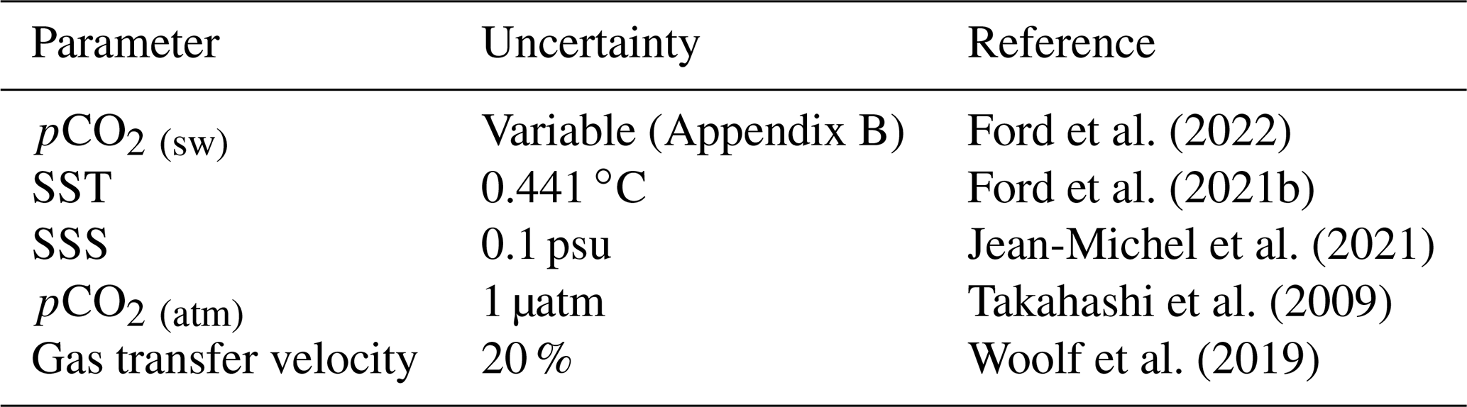
The approach was applied to monthly 1^∘ fields of ΔpCO₂ that were estimated from pCO_2  (atm) and SA-FNN pCO_2  (sw) on a per pixel basis. The pCO_2  (atm) and spatially and temporally varying pCO_2  (sw) uncertainties (Table 1; Fig. B1) were propagated through the X-11 analysis, using a Monte Carlo uncertainty propagation approach. The input time series were randomly perturbed 1000 times within the uncertainties of each parameter, and Spearman correlations were calculated for each perturbation. The 95 % confidence interval was extracted from the resulting distribution of correlation coefficients, and results were deemed significant (α<0.05) where the confidence interval remained significant. Spatial autocorrelation was tested using the method of field significance (Wilks, 2006). The analysis was then conducted on the CO₂ fluxes on a per pixel basis. The pCO_2  (sw), pCO_2  (atm), gas transfer velocity, SST, and SSS uncertainties (Table 1) were propagated through the flux calculations using the same Monte Carlo uncertainty propagation approach used for ΔpCO₂.

The potential drivers tested were MODIS-A skin SST, NCP, and NPP alongside SSS from the CMEMS global reanalysis product (GLORYSV12; CMEMS, 2021) and two climate indices: multivariate El Niño–Southern Oscillation (ENSO) index (MEI) as an indicator of ENSO phases from https://www.esrl.noaa.gov/psd/enso/mei (last access: 19 December 2019) and Southern Annular Mode (SAM) data, which indicate the displacement of the westerly winds in the Southern Ocean and were downloaded from http://www.nerc-bas.ac.uk/icd/gjma/sam.html (last access: 19 December 2019).

Table 1 Uncertainties in the input parameters used in the Monte Carlo uncertainty propagation.

2.5 Trend analysis

The linear trends in the inter-annual components of ΔpCO₂ and the CO₂ flux were calculated on a per pixel basis using the non-parametric Mann–Kendall test (Kendall, 1975; Mann, 1945) and Sen's slope estimates (Sen, 1968), which are less sensitive to outliers in the time series. The input parameter uncertainties (Table 1) were propagated within this trend analysis using a Monte Carlo uncertainty propagation (n=1000) to extract the 95 % confidence interval on the trends. The overall trend was deemed significant if 95 % of the trends were significant (α=0.05), and the uncertainties in these trends are displayed in Appendix B (Fig. B2).

2.6 Limitations

It should be noted that correlations between the ΔpCO₂ and SST and NCP are expected since the SA-FNN estimates pCO_2  (sw) (the major determinant of ΔpCO₂ variability) using SST and NCP as input parameters which are subsequently interpreted as drivers here. By extension, but to a lesser extent, this also applies to correlations between CO₂ flux and SST and NCP since pCO_2  (sw) is included in the flux calculations. Different lines of evidence suggest that this is not a major limitation of our study. Firstly, any correlation between Δ$p{\mathrm{CO}}_{\mathrm{2}}/{\mathrm{CO}}_{\mathrm{2}}$ flux and SST and NCP is not determined a priori but is an emerging property of the SA-FNN. Therefore, the driver analysis undertaken here represents an indirect decomposition of the SA-FNN drivers rather than a strict correlation analysis between independent variables. The accurate representation of seasonal pCO_2  (sw) cycles across the South Atlantic Ocean (Ford et al., 2022) provides confidence in the SA-FNN. Secondly, conducting the analysis described by Henson et al. (2018) using in situ pCO_2  (sw) to estimate ΔpCO₂ on a per province basis (Longhurst, 1998) for the South Atlantic Ocean yielded similar seasonal drivers to the SA-FNN (Appendix A). The inter-annual drivers displayed some differences, however, which may be due to the spatial and temporal averaging that is required to construct the in situ time series.

3 Results

3.1 Seasonal drivers of ΔpCO₂ and CO₂ flux

The X-11 analysis conducted on ΔpCO₂ indicated significant seasonal correlations (Fig. 1) when the uncertainties are accounted for. The subtropics (10 to 40^∘ S) showed positive correlations between ΔpCO₂, SST, and SSS (Fig. 1c, d), as well as negative correlations between ΔpCO₂, NCP, and NPP (Fig. 1a, b). In contrast the subpolar (south of 40^∘ S) and equatorial regions (10^∘ N to 10^∘ S) displayed negative correlations between ΔpCO₂ and SST (Fig. 1c). Correlations between ΔpCO₂ and NCP were negative in the subpolar regions and were positive in the equatorial regions (Fig. 1a). There were no significant correlations observed between ΔpCO₂ and MEI or SAM in any of the regions.

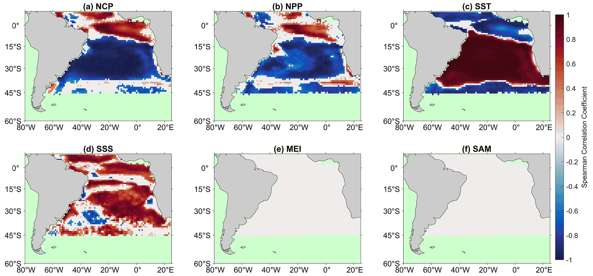
Figure 1 Significant Spearman correlations between the ΔpCO₂ seasonal component of the X-11 analysis and (a) net community production (NCP), (b) net primary production (NPP), (c) sea surface temperature (SST), (d) sea surface salinity (SSS), (e) multivariate ENSO index (MEI), and (f) Southern Annular Mode (SAM) seasonal components. White regions indicate no significant correlations, and green regions indicate no analysis was performed due to missing satellite data.

Regional deviations were observed in the Amazon plume, Benguela upwelling, the South American coast, and a band across 40^∘ S. The region under the influence of the Amazon plume indicated negative correlations between ΔpCO₂ and NCP in contrast to the surrounding waters which had positive correlations (Fig. 1a). The Benguela upwelling displayed positive correlations between ΔpCO₂ and NCP (Fig. 1a), no significant correlations between ΔpCO₂ and SST (Fig. 1c), and negative correlations between ΔpCO₂ and SSS (Fig. 1e). The South American coast between 12 and 17^∘ S displayed positive correlations between ΔpCO₂ and NPP (Fig. 1b), along with negative correlations between ΔpCO₂ and SSS (Fig. 1e). Negative correlation between ΔpCO₂ and SSS and positive correlations between NCP, NPP, and ΔpCO₂ were also observed in the southwestern Atlantic (Fig. 1e). Positive correlations between NCP, NPP, and ΔpCO₂ were identified in a band across 40^∘ S (Fig. 1a, b). Performing the X-11 analysis on the CO₂ flux revealed similar and comparable correlations to ΔpCO₂ (Fig. 2). Significant driver–flux correlations were observed over a larger area compared to ΔpCO₂, however.

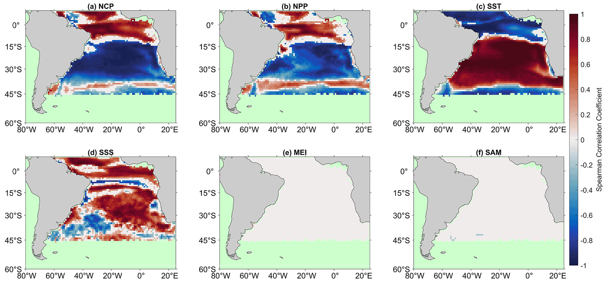
Figure 2 Significant Spearman correlations between the air–sea CO₂ flux seasonal component of the X-11 analysis and (a) net community production (NCP), (b) net primary production (NPP), (c) sea surface temperature (SST), (d) sea surface salinity (SSS), (e) multivariate ENSO index (MEI), and (f) Southern Annular Mode (SAM) seasonal components. White regions indicate no significant correlations, and green regions indicate no analysis was performed due to missing satellite data.

3.2 Inter-annual drivers of ΔpCO₂ and CO₂ flux

The X-11 analysis identified regionally significant inter-annual correlations between ΔpCO₂ and SST, MEI, and to a lesser extent NCP and SSS (Fig. 3). The subtropics displayed positive correlations between SST and ΔpCO₂, which extended across the basin from the South American coast (Fig. 3c). Positive correlations were also observed between the MEI and ΔpCO₂ (Fig. 3e), with a similar geographic extent to the correlations with SST. In the central South Atlantic gyre spatially variable negative correlations between NCP and ΔpCO₂ and positive correlations between SSS and ΔpCO₂ were observed (Fig. 3a, d). The central equatorial Atlantic displayed spatially variable positive correlations between NCP and ΔpCO₂, which extended southeast towards the African coast (Fig. 3a).

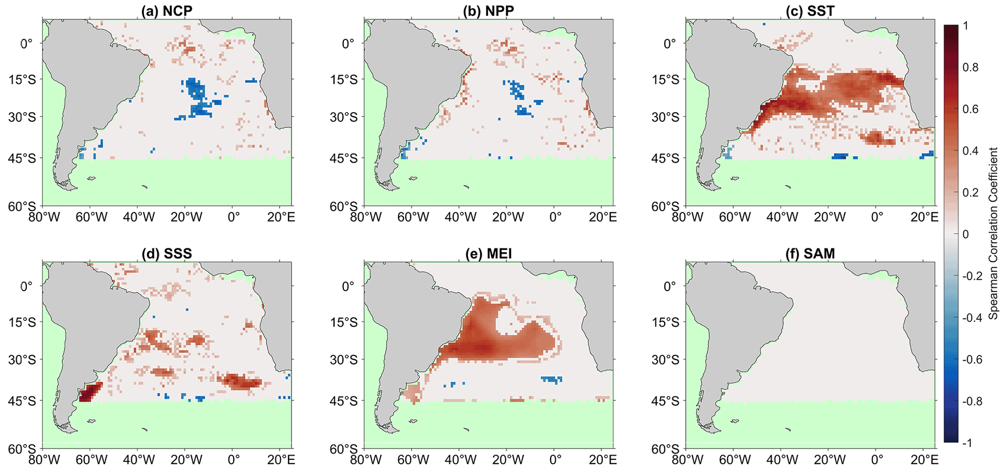
Figure 3 Significant Spearman correlations between the ΔpCO₂ inter-annual component of the X-11 analysis and (a) net community production (NCP), (b) net primary production (NPP), (c) sea surface temperature (SST), (d) sea surface salinity (SSS), (e) multivariate ENSO index (MEI), and (f) Southern Annular Mode (SAM) inter-annual components. White regions indicate no significant correlations, and green regions indicate no analysis was performed due to missing satellite data.

Significant inter-annual correlations for the CO₂ flux were also identified by the X-11 analysis (Fig. 4), which generally covered a larger spatial area to the corresponding ΔpCO₂ correlations (Fig. 3). Positive correlations between the CO₂ flux and SST were observed in the subtropics (Fig. 4c), consistent with the correlations with ΔpCO₂ (i.e. by comparing Figs. 4c and 3c). Nevertheless, negative correlations between the CO₂ flux and SST were observed at the border between the equatorial region and subtropics, which was not identified in the ΔpCO₂ correlations. Negative correlations between NCP and the CO₂ flux were also identified over a spatially larger area (Figs. 4a, 3a). Correlations between the MEI and CO₂ flux were positive in the subtropics (Fig. 4e) and included a band of negative correlations to the south between 35 and 45^∘ S (Fig. 4e).

Figure 4 Significant Spearman correlations between the air–sea CO₂ flux inter-annual component of the X-11 analysis and (a) net community production (NCP), (b) net primary production (NPP), (c) sea surface temperature (SST), (d) sea surface salinity (SSS), (e) multivariate ENSO index (MEI), and (f) Southern Annular Mode (SAM) inter-annual components. White regions indicate no significant correlations, and green regions indicate no analysis was performed due to missing satellite data.

Positive correlations between NCP and CO₂ flux were observed in the western equatorial Atlantic, alongside spatially variable negative correlations to SST (Fig. 4a, c). Positive correlations between SSS and CO₂ flux were identified in the region of the Amazon plume (Fig. 4d). Weak positive correlations between the SAM and CO₂ flux were identified between 30 and 45^∘ S (Fig. 4f).

3.3 Trends in inter-annual ΔpCO₂ and CO₂ flux

Regions of significant trends in the inter-annual component of ΔpCO₂ were observed (Fig. 5a). Negative trends occurred in the South Atlantic gyre. Positive trends in ΔpCO₂ were identified along the South African coast, which switched to strong negative trends moving offshore into the central South Atlantic gyre. Positive trends were also observed in the equatorial Atlantic consistent with the positions of the Amazon plume and equatorial upwelling.

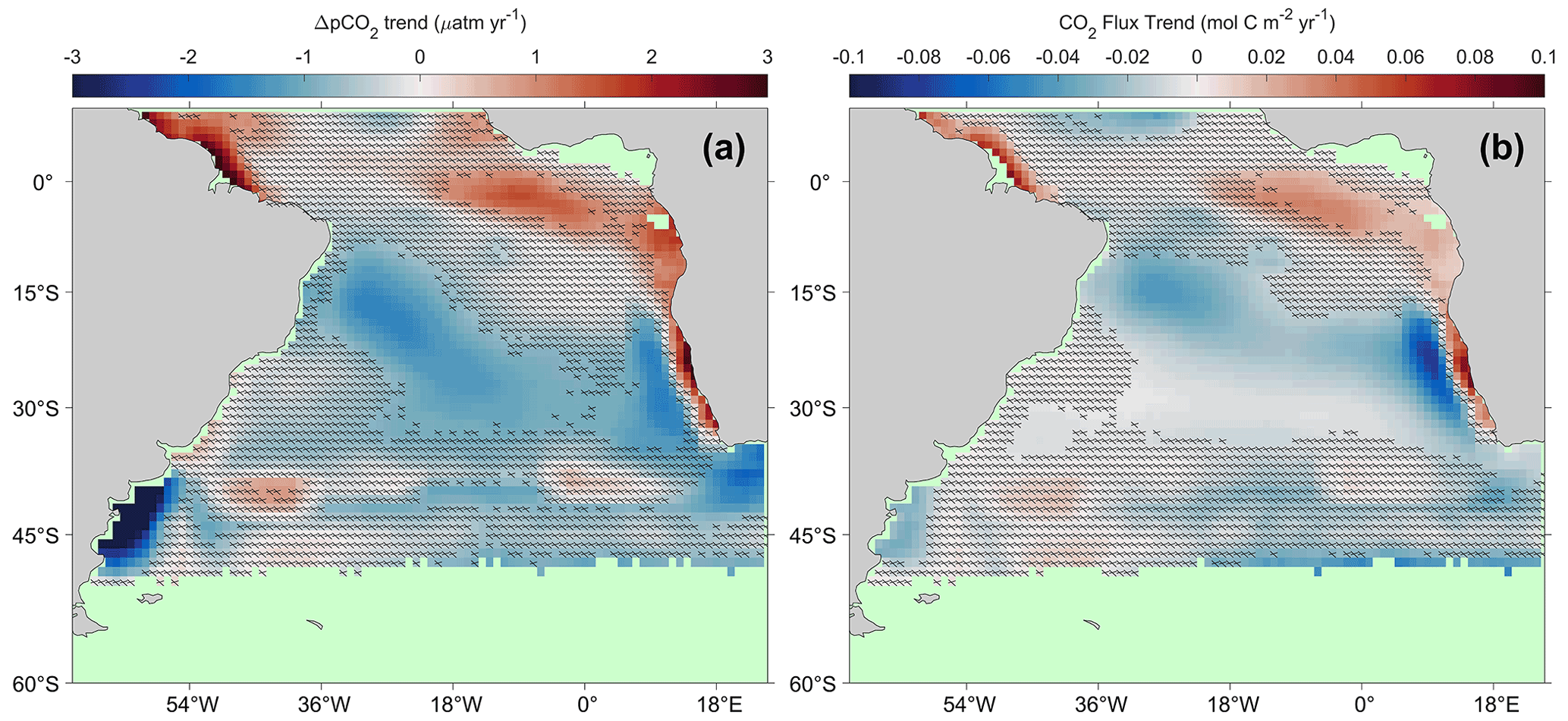
Figure 5 Linear trends in (a) ΔpCO₂ and (b) the air–sea CO₂ flux between 2002 and 2018. Hashed areas indicate non-significant trends when accounting for the uncertainties. Green regions indicate insufficient data to calculate trends.

Regions of significant trends in the CO₂ flux were identified (Fig. 5b) but over much larger spatial areas than evident in the ΔpCO₂ results (i.e. comparing Fig. 5a with 5b). The trends in CO₂ flux are generally in the same direction as trends in ΔpCO₂. Strong positive trends in the CO₂ flux occurred in the Benguela upwelling region and switched to a negative trend offshore of similar magnitude but occupied a larger spatial area.

4 Discussion

4.1 Seasonal drivers of ΔpCO₂ and CO₂ flux

Previous studies have explored the seasonal drivers of ΔpCO₂ and to a lesser extent the air–sea CO₂ flux. In this study, we investigated the drivers of ΔpCO₂ and CO₂ flux at both seasonal and inter-annual timescales in the South Atlantic Ocean. In the North Atlantic, Henson et al. (2018) indicated that the seasonal variability in subtropical ΔpCO₂ variability is driven by SST, whereas the variability in ΔpCO₂ in subpolar regions is biologically driven, similar to previous studies (Takahashi et al., 2002; Landschützer et al., 2013). The X-11 analysis conducted on spatially complete ΔpCO₂ and CO₂ flux displayed consistent seasonal results (Figs. 1, 2), though for the CO₂ flux significant correlations occupied a larger area. These both indicated a similar pattern in seasonal drivers for the South Atlantic Ocean, with subtropical ΔpCO₂ and CO₂ flux driven by SST and subpolar correlated with biological controls, although the equatorial region exhibited more complex patterns (Fig. 1).

In the equatorial Atlantic, the correlations between ΔpCO₂, SST, and biological production were spatially variable (Fig. 1). Landschützer et al. (2013) suggested that the temperature and non-temperature (i.e. biological and circulation) drivers generally compensated each other. We found positive correlations between the NCP, ΔpCO₂, and CO₂ flux seasonal components, indicating that biological activity is likely a key driver of seasonal variability in response to the equatorial upwelling. Ford et al. (2022) showed that the SA-FNN improved the seasonal pCO_2  (sw) variability in the equatorial Atlantic compared to the current “state of the art” SOM-FNN methodology (Watson et al., 2020). Elevated ΔpCO₂ associated with elevated NCP in the eastern equatorial Atlantic was consistent with the seasonal equatorial upwelling (Radenac et al., 2020). Parard et al. (2010) indicated strong negative correlations between SST and ΔpCO₂ during the upwelling season ($R=-\mathrm{0.76}$ for June to September), which is also consistent with our results. By contrast, Lefèvre et al. (2016) showed that correlations between pCO_2  (sw) and SST were weak across the whole year ($R=-\mathrm{0.13}$), and SSS (R=0.93) was the primary driver at the same station.

In the western equatorial Atlantic, negative correlations between NCP and ΔpCO₂ and positive correlations between the SSS and ΔpCO₂ seasonal component occurred in the vicinity of the Amazon River mouth. The mixing of the Amazon River and oceanic water decreases SSS (Ibánhez et al., 2016; Lefèvre et al., 2020; Bonou et al., 2016; Lefévre et al., 2010) and increases the nutrient supply to the ocean which can in turn enhance NPP and NCP, leading to a decrease in ΔpCO₂ within the Amazon plume (Körtzinger, 2003; Cooley et al., 2007). This coupling produces an extensive area of depressed ΔpCO₂ which is a CO₂ sink (Ibánhez et al., 2016). Lefèvre et al. (2010) indicated that rainfall from the intertropical convergence zone could reduce SSS, with an associated decrease in ΔpCO₂. The eastern Tropical Atlantic is also subject to large river input, especially from the Congo (Hopkins et al., 2013) and Niger rivers, which could produce nutrient-rich plumes that fuel NCP and decrease ΔpCO₂ (Lefèvre et al., 2016, 2021).

Between 30 and 45^∘ S, dissolved inorganic carbon and SST exert a similar influence on pCO_2  (sw), indicating that seasonal changes in dissolved inorganic carbon driven by biological uptake in the summer and upwelling in winter are approximately balanced by seasonal changes in SST and their control on the solubility pump (Henley et al., 2020). This most likely explains the band of positive correlations between NCP, NPP, and ΔpCO₂ and sharp transitions in correlations between SST and ΔpCO₂ across ∼ 40^∘ S.

Deviations from the expected drivers in the subtropics, occurred within the Benguela upwelling system between 20 and 35^∘ S. Positive correlations between NCP and the CO₂ flux (Fig. 2a) alongside negative correlations between SST, SSS, and the CO₂ flux (Fig. 2c, d) are indicative of upwelled waters that have both elevated pCO_2  (sw) and nutrients, which cause an increase in NPP (Lamont et al., 2014). These upwelled waters move offshore in filaments (Rubio et al., 2009) where NPP decreases and SST becomes the dominant driver, which is confirmed by the positive correlations between SST and the CO₂ flux further offshore. Ford et al. (2021b) indicated a switch in NCP drivers in the Benguela upwelling from wind-driven upwelling on the shelf to filaments that propagate offshore from the upwelling front, which is consistent with the switch in the drivers observed for the CO₂ flux as these filaments move offshore.

At between 12 and 17^∘ S along the South American coast, there were also deviations from the expected drivers as there were positive correlations between NPP and ΔpCO₂ (Fig. 1b) and negative correlations between SSS and ΔpCO₂ (Fig. 1d), which are consistent with an upwelling signature that occurs along the coast. Aguiar et al. (2018) also showed intense seasonal upwelling events in this region that are driven by wind and currents. The southern coast of South America is strongly influenced by riverine water input that reduces the total alkalinity and therefore causes an increase in pCO_2  (sw) (Liutti et al., 2021). This is associated with an increased supply of nutrients which in turn enhances NPP, though the main drivers of pCO_2  (sw) in this region are still total alkalinity and SST (Liutti et al., 2021). This potentially explains the positive correlation between ΔpCO₂ and both NCP and NPP (Fig. 1a, b), as well as the negative correlations between ΔpCO₂ and SSS. The extension offshore of this negative correlation between SSS and ΔpCO₂ (Fig. 1d) could be caused by the advection of water masses due to intense mesoscale eddy activity arising from the Brazil–Malvinas confluence (Mason et al., 2017).

The seasonal correlations between the CO₂ flux and the drivers were similar to ΔpCO₂, but for CO₂ flux these occurred over a larger spatial area. The South Atlantic subtropical anticyclone which controls wind speeds across the region (Reboita et al., 2019) and therefore the gas transfer velocity could enhance the CO₂ flux into the subtropical ocean through higher (or lower) wind speeds in winter (or summer; Xiong et al., 2015). Since seasonal variations in ΔpCO₂ largely explain the seasonal variability in the CO₂ flux, ΔpCO₂ can be used as a proxy to understand seasonal variations in the CO₂ flux in this region.

4.2 Inter-annual drivers of ΔpCO₂ and CO₂ flux

The larger geographic region of significant correlations for the air–sea CO₂ flux compared to ΔpCO₂ and the consistency between the two results (i.e. comparing the smaller regions of ΔpCO₂ correlations with their equivalent in the flux results; Figs. 3, 4) suggest that analysing the CO₂ flux is the better dataset to investigate drivers of variations on inter-annual and longer timescales. The results become clearer when analysing the CO₂ flux, in which the effects of solubility and gas transfer (estimated via wind speed proxy) could reinforce correlations and multi-year trends, which will be retrieved by performing long time series analyses on the CO₂ flux. Landschützer et al. (2015) showed that variations in the Southern Ocean carbon sink were primarily driven by changes in ΔpCO₂, when integrating across basin scales. At localized scales of 1^∘ by 1^∘ as performed in our analysis, changes in surface turbulence and solubility are shown to be important in determining inter-annual variability, consistent with Keppler and Landschützer (2019). In the North Atlantic Ocean, Henson et al. (2018) showed that the seasonal and inter-annual drivers of ΔpCO₂ are different, which could arise from the necessity to study CO₂ fluxes over longer timescales.

The inter-annual component of NCP and the CO₂ flux were negatively correlated in the subtropical gyre (Fig. 4a), alongside a positive correlation between SST and CO₂ flux (Fig. 4b). El Niño (La Niña) events are known to influence the South Atlantic Ocean, causing an increase (decrease) in SST across the basin (Rodrigues et al., 2015; Colberg et al., 2004) and a decrease (increase) in NPP and NCP (Ford et al., 2021b; Tilstone et al., 2015). Positive correlations between the MEI and CO₂ flux (Fig. 4e) indicate that the MEI partially controls the inter-annual variability in CO₂ flux in the South Atlantic subtropical gyre through modulations primarily in SST and to a lesser extent NCP. The South Atlantic Subtropical Anticyclone has been observed to strengthen (weaken) and move south (north) during La Niña (El Niño) events. This displacement increases (decreases) wind speeds across the subtropical South Atlantic, which will enhance (weaken) gas exchange and elevate (depress) NCP (Ford et al., 2021b). These results suggest a more significant role of NCP in controlling the inter-annual variability in the CO₂ flux than has previously been thought.

The negative correlation between the CO₂ flux and the MEI in a band between 30 and 45^∘ S (Fig. 4e) indicates that reduced (elevated) wind speeds that occur during La Niña (El Niño) events in this region suppress (enhance) the gas exchange (Colberg et al., 2004) and therefore act as a weaker (stronger) CO₂ sink. In the equatorial region, neither ΔpCO₂ or the CO₂ flux were correlated with the MEI, in sharp contrast with Lefèvre et al. (2013) who showed stronger outgassing of CO₂ in the western equatorial Atlantic for the year following the 2009 El Niño. In that respect, it should be noted that our analysis would not identify such lagged correlations.

The SAM has known meteorological connections to the MEI (Fogt et al., 2011), in which El Niño (La Niña) events generally coincide with negative (positive) SAM phases, resulting in northward (southward) displacement of the westerly winds in the Southern Ocean. Our results showed positive correlations between the CO₂ flux and the SAM between 30 and 45^∘ S (Fig. 4f) indicating stronger (weaker) CO₂ drawdown into the oceans during negative (positive) SAM phases. Although no significant correlations were found between ΔpCO₂ and the SAM (Fig. 3f), the changes in the gas transfer driven by the displacement of the westerly winds could control the CO₂ flux. It should be noted that the effect of the SAM may be more pronounced outside the domain of the present study (i.e. south of 45^∘ S; Keppler and Landschützer, 2019). Landschützer et al. (2015) indicated that the SAM is unlikely to be the main driver of changes in the Southern Ocean CO₂ flux, but an observed zonally asymmetric atmospheric pattern could induce changes in the CO₂ flux (Keppler and Landschützer, 2019; Landschützer et al., 2015). This asymmetric atmospheric pattern, however, may not be captured within the SAM index.

4.3 Multi-year trends in ΔpCO₂ and CO₂ flux

The trends in ΔpCO₂ and CO₂ flux over 16 years (Fig. 5) showed some similarities to previous trend assessments in the South Atlantic Ocean (Landschützer et al., 2016). Our results indicated a lower number of significant trends, however, since uncertainties in the trend analysis were accounted for. The uncertainties in both the pCO_2  (sw) estimates from extrapolation techniques and the gas transfer velocity are rarely propagated through previous trend analyses. By accounting for these uncertainties, the trend analyses provide a robust depiction of regions that can confidently be determined as changing. As with the seasonal and inter-annual analysis, the CO₂ flux-based trend analysis showed a greater spatial area of significant trends when compared to ΔpCO₂ (Fig. 5).

The strongest trends in ΔpCO₂ and the CO₂ flux were observed in the Benguela upwelling system. Arnone et al. (2017) reported positive trends in in situ pCO_2  (sw) of 6.1 ± 1.4 µatm yr⁻¹, between 2005 and 2015. Assuming an atmospheric CO₂ increase of 1.5 µatm yr⁻¹ (Takahashi et al., 2002; Zeng et al., 2014), these results are consistent with the ΔpCO₂ trends observed in this study (1.5 ± 1.1–3.8 ± 1.1  µatm yr⁻¹, Fig. 5a). Arnone et al. (2017) also suggested that the positive trend was due to a stronger influence of upwelling (Rouault et al., 2010), which injects CO₂ and nutrients into the area that is then not completely removed by the enhanced NPP/NCP. Varela et al. (2015) indicated an increase in the strength of the Benguela upwelling. By contrast, Lamont et al. (2018) showed no significant change in upwelling in the southern Benguela but increases in the northern Benguela that are consistent with our data, which highlight an increasing efflux of CO₂ to the atmosphere (Fig. 5b). The CO₂ flux trends in this study (0.03 ± 0.01–0.09 ± 0.02 mol m⁻² yr⁻¹, Fig. 5b) were also consistent with but slightly lower than the 0.13 ± 0.03 mol m⁻² yr⁻¹ trend in CO₂ flux observed by Arnone et al. (2017). An increase in the strength of the upwelling that injects CO₂ into the surface layer will be driven by enhanced (upwelling-conducive) winds that also enhance the gas transfer. This highlights the importance of studying multi-year trends using the CO₂ flux because the enhancement of these trends by meteorological conditions would not be observed using ΔpCO₂ alone.

Offshore from the upwelling region negative ΔpCO₂ and CO₂ flux trends were observed. Rubio et al. (2009) showed that mesoscale filaments and eddies propagate away from the upwelling front, transporting nutrients offshore into the South Atlantic gyre. Ford et al. (2021b) showed negative correlations between sea level height anomalies (SLHAs) and NPP/NCP anomalies (negative SLHAs; positive NCP/NPP), indicating an influence of mesoscale features on ΔpCO₂ and the CO₂ flux. Xiu et al. (2018) indicated that an increase in upwelling-conducive winds could increase the number of mesoscale eddies, which would transport nutrients offshore of the Californian upwelling. Although the Benguela and Californian upwelling systems are not identical, these connections could suggest an elevated nutrient export offshore, driving elevated NPP/NCP, which would increase the CO₂ sink. Kulk et al. (2020) showed significant increases in NPP of ∼ 2 % yr⁻¹ between 1998 and 2018 in the region of strong negative trends in the CO₂ flux observed in this study, which supports the contribution of NCP to multi-year trends in the CO₂ flux.

There were also positive trends in ΔpCO₂ and CO₂ flux in the equatorial Atlantic. In the eastern equatorial Atlantic, Lefèvre et al. (2016) previously suggested a negative trend in in situ ΔpCO₂, between 2006 and 2013, but indicated that the trend may be biased by extreme events at either end of the record. From 1995 to 2007, Parard et al. (2010) indicated a greater increase in in situ pCO_2  (sw) than pCO_2  (atm) (increasing ΔpCO₂), but the trend was derived from data from only two research cruises. For the equatorial upwelling, an increase in ΔpCO₂ (as shown here and in Landschützer et al., 2016) is counter intuitive because there is evidence that upwelled water has recently been in contact with the atmosphere (∼ 15 years; Reverdin et al., 1993). Dissolved inorganic carbon in these upwelled waters has been shown to increase at a similar rate to the surface waters (e.g. Woosley et al., 2016). Therefore, the trend in ΔpCO₂ should be ∼ 0 with increasing pCO_2  (atm). This could suggest a missing component within the SA-FNN to estimate pCO_2  (sw), such as changes in the biological export efficiency (Kim et al., 2019), which could then suppress upwelling-induced CO₂ outgassing.

The western Tropical Atlantic, in the vicinity of the Amazon plume, also showed positive trends in ΔpCO₂ and CO₂ flux. Previous studies have not investigated the trends in ΔpCO₂ or CO₂ flux in the Amazon plume; however, the carbon retention in a coloured ocean site (CARIACO), situated to the northwest, displayed positive trends in pCO_2  (sw) of 2.95 ± 0.43 µatm yr⁻¹ (Bates et al., 2014). Araujo et al. (2019) identified a positive trend in pCO_2  (sw) of 1.20 µatm yr⁻¹ but a trend in pCO_2  (atm) of 1.70 µatm yr⁻¹ (i.e. decreasing ΔpCO₂) for the northeast Brazilian coast, although the air–sea CO₂ flux and ΔpCO₂ within the Amazon plume region are spatially and temporally variable (Valerio et al., 2021; Ibánhez et al., 2016; Bruto et al., 2017).

The South Atlantic gyre exhibited negative trends in ΔpCO₂ and the CO₂ flux indicating an increasing drawdown of atmospheric CO₂ into the ocean, which were consistent with Landschützer et al. (2016) over the period from 1982 and 2011 though the trends were at the limits of the uncertainties (Fig. B2). Fay and Mckinley (2013) showed weak negative trends in ΔpCO₂ using in situ observations over different time series lengths. Using an ensemble of complete pCO_2  (sw) fields, Gregor et al. (2019) indicated negative trends in ΔpCO₂; however, there was low confidence in these trends especially in the South Atlantic gyre. By contrast, Kitidis et al. (2017) reported a mean trend in in situ ΔpCO₂ between 1995 and 2013 that was not significantly different from zero. These contradictory trends support the conclusion that ΔpCO₂ is unlikely to be representative of the CO₂ flux over multi-year timescales. Therefore, we recommend that the CO₂ flux should be used to assess multi-year variability in the oceanic CO₂ sink, as the importance of changes in solubility and gas transfer velocity (estimated via wind speed) increases (Keppler and Landschützer, 2019).

During the United Nations decade of ocean science (2021–2030) , the Integrated Ocean Carbon Research (IOC-R) highlights that the role of biology is a key issue to understanding the global ocean CO₂ sink (Aricò et al., 2021). The biological contribution to both inter-annual and multi-year variations in the South Atlantic air–sea CO₂ flux shown in this study, and supported by Ford et al. (2022), indicates that the biological activity through NCP cannot be assumed to be in steady state. The biological effect of NCP on ΔpCO₂ and CO₂ flux should therefore not be overlooked when assessing the inter-annual and multi-year variations in the global ocean carbon sink.

5 Conclusions

In this paper, we have investigated the seasonal and inter-annual drivers of ΔpCO₂ and the air–sea CO₂ flux in the South Atlantic Ocean using satellite observations. Seasonally, our results indicated that the subtropics were controlled by SST, and the subpolar regions were correlated with biological processes. Deviations from this trend occurred in the Benguela upwelling where predominately biological processes correlated with variability in the ΔpCO₂, as well as upwelling. The equatorial Atlantic showed spatially variable drivers associated with the Amazon plume and equatorial upwelling which induced a biological effect. These regions imply a strong biological control on ΔpCO₂ through local physical processes. The CO₂ flux had similar seasonal drivers to ΔpCO₂ but with significant correlations over a larger spatial area. This highlights that ΔpCO₂ can be used to indicate the important drivers of the CO₂ flux on seasonal timescales, but it is still possible that ΔpCO₂ will miss some of the spatial correlations and will likely overestimate the strength of these correlations.

The inter-annual variability in ΔpCO₂ and the CO₂ flux was correlated with the MEI through a reduction (increase) of NCP and increase (decrease) in SST during El Niño (La Niña) events, again highlighting the importance of biology to the inter-annual variability. The CO₂ flux response extended over a larger geographical region, indicating that the CO₂ flux should be used to assess inter-annual trends in the oceanic CO₂sink, as opposed to a proxy such as ΔpCO₂, which may overestimate the strength of the correlations and does not include variability in the solubility and the gas transfer velocity (estimated via wind speed). The 16-year trends in ΔpCO₂ and the CO₂ flux were determined with associated uncertainties which identified negative trends in the CO₂ flux in the South Atlantic gyre. Positive trends in the CO₂ flux were observed in the Benguela upwelling region, which were associated with an increase in the strength and frequency of upwelling. A transition to negative trends offshore were consistent with elevated nutrient export from the upwelling area and subsequent biological drawdown of CO₂. These results highlight that changes in biological activity in the South Atlantic Ocean can control the inter-annual and multi-year trends in the oceanic CO₂ flux. This emphasizes the importance of biology and specifically NCP in assessing the global ocean carbon sink.

Appendix A: Driver analysis using in situ ΔpCO₂

Henson et al. (2018) performed the X-11 analysis using in situ pCO_2  (sw) observations to estimate average ΔpCO₂ for the Longhurst provinces (Longhurst, 1998). The in situ pCO_2  (sw) observations were obtained from SOCATv2020 (https://www.socat.info/, last access: 16 June 2020; Bakker et al., 2016) and were reanalysed to a temperature dataset representative of a consistent and fixed depth (Reynolds et al., 2002) which is used to represent the base of the mass boundary layer. The reanalysis method used the “fe_reanalyse_socat.py” routine within FluxEngine (Holding et al., 2019; Shutler et al., 2016), which follows the methodology of Goddijn-Murphy et al. (2015) and that used in Woolf et al. (2019) and Watson et al. (2020). ΔpCO₂ was calculated using the reanalysed in situ pCO_2  (sw) observations and pCO_2  (atm). These ΔpCO₂ estimates were used within the driver analysis as described by Henson et al. (2018), using the drivers described in Sect. 2.4 for the South Atlantic Longhurst provinces (Longhurst, 1998). The seasonal drivers of in situ ΔpCO₂ (Fig. A1) showed a similar spatial distribution as the SA-FNN ΔpCO₂ (Fig. 1). The inter-annual drivers (Fig. A2) showed some differences to the SA-FNN (Fig. 3). The averaging required to produce the in situ ΔpCO₂ time series may mask inter-annual signals, and Ford et al. (2021b) indicated that averaging over large province areas could mask correlations, especially in dynamic regions, and locally these correlations may be significant.

Figure A1 Spearman correlations between the in situ ΔpCO₂ seasonal component of the X-11 analysis and (a) net community production (NCP), (b) net primary production (NPP), (c) sea surface temperature (SST), (d) sea surface salinity (SSS), (e) multivariate ENSO index (MEI), and (f) Southern Annular Mode (SAM) seasonal components on a per province basis. Hashed areas indicate no significant correlations, and green regions indicate no analysis was performed due to missing data.

Figure A2 Spearman correlations between the in situ ΔpCO₂ inter-annual component of the X-11 analysis and (a) net community production (NCP), (b) net primary production (NPP), (c) sea surface temperature (SST), (d) sea surface salinity (SSS), (e) multivariate ENSO index (MEI), and (f) Southern Annular Mode (SAM) inter-annual components on a per province basis. Hashed areas indicate no significant correlations, and green regions indicate no analysis was performed due to missing data.

Appendix B: SA-FNN pCO_2  (sw) and trend uncertainties

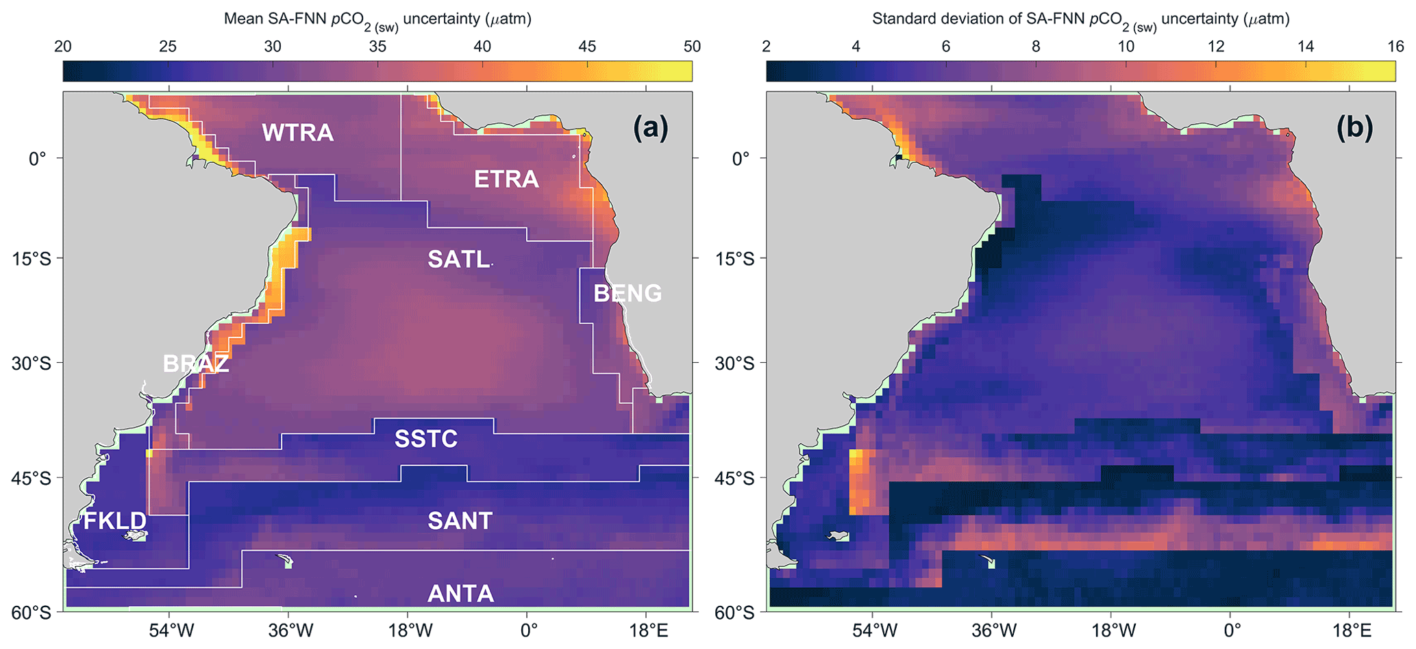
Figure B1 (a) Mean SA-FNN pCO_2  (sw) uncertainty between July 2002 and December 2018. Longhurst provinces (Longhurst, 1998) used within the SA-FNN training described in Ford et al. (2022; note the WTRA and ETRA are merged into one province). The province area acronyms are listed as follows: WTRA is western tropical Atlantic, ETRA is eastern equatorial Atlantic, SATL is South Atlantic gyre, BRAZ is the coastal Brazilian Current, BENG is Benguela Current coastal upwelling, FKLD is southwest Atlantic shelves, SSTC is South Subtropical Convergence, SANT is sub-Antarctic, and ANTA is Antarctic. (b) Standard deviation of SA-FNN pCO_2  (sw) uncertainty.

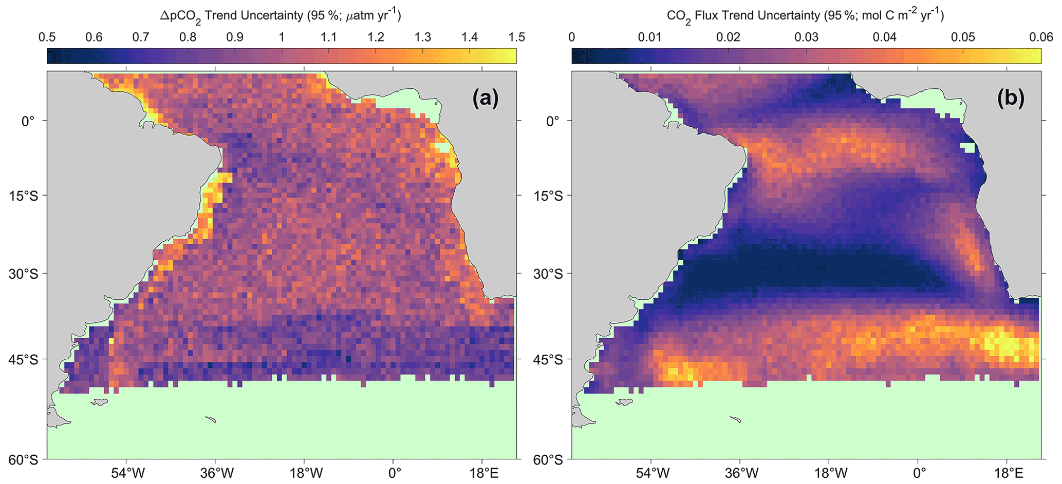
Figure B2 (a) Uncertainty in the ΔpCO₂ trends presented in Fig. 5a. (b) Uncertainty in the air–sea CO₂ flux trends presented in Fig. 5b.