Spatial and temporal variation in δ¹³C values of methane emitted from a hemiboreal mire: methanogenesis, methanotrophy, and hysteresis

The reasons for spatial and temporal variation in methane emission from mire ecosystems are not fully understood. Stable isotope signatures of the emitted methane can offer clues to the causes of these variations. We measured the methane emission ($F_{{\mathrm{CH}}_{\mathrm{4}}})$ and ¹³C signature (δ¹³C) of emitted methane by automated chambers at a hemiboreal mire for two growing seasons. In addition, we used ambient methane mixing ratios and δ¹³C to calculate a mire-scale ¹³C signature using a nocturnal boundary-layer accumulation approach. Microbial methanogenic and methanotrophic communities were determined by a captured metagenomics analysis. The chamber measurements showed large and systematic spatial variations in δ¹³C-CH₄ of up to 15 ‰ but smaller and less systematic temporal variation. According to the spatial δ¹³C–$F_{{\mathrm{CH}}_{\mathrm{4}}}$ relations, methanotrophy was unlikely to be the dominating cause for the spatial variation. Instead, these were an indication of the substrate availability of methanogenesis being a major factor in explaining the spatial variation. Genetic analysis indicated that methanogenic communities at all sample locations were able to utilize both hydrogenotrophic and acetoclastic pathways and could thus adapt to changes in the available substrate. The temporal variation in $F_{{\mathrm{CH}}_{\mathrm{4}}}$ and δ¹³C over the growing seasons showed hysteresis-like behavior at high-emission locations, indicative of time-lagged responses to temperature and substrate availability. The upscaled chamber measurements and nocturnal boundary-layer accumulation measurements showed similar average δ¹³C values of −81.3 ‰ and −79.3 ‰, respectively, indicative of hydrogenotrophic methanogenesis at the mire. The close correspondence of the δ¹³C values obtained by the two methods lends confidence to the obtained mire-scale isotopic signature. This and other recently published data on δ¹³C values of CH₄ emitted from northern mires are considerably lower than the values used in atmospheric inversion studies on methane sources, suggesting a need for revision of the model input.

1 Introduction

Methane (CH₄) is one of the three main drivers of anthropogenic climate change. Its sources include both biological and anthropogenic processes, with the most significant natural source being wetland ecosystems (Ciais et al., 2013). As changing climate may influence global CH₄ emission from wetlands, a mechanistic understanding of the processes behind these emissions is crucial.

The CH₄ emission rates from wetlands are controlled by CH₄ production (methanogenesis), CH₄ oxidation (methanotrophy), and the transport of CH₄ from peat into the atmosphere (e.g., Lai, 2009). A fundamental factor for CH₄ production by Archaea is the availability of substrates, as H₂ or acetate for hydrogenotrophic or acetoclastic methanogenesis, respectively (e.g., Lai, 2009). Furthermore, temperature is a key driver of the CH₄ emission rate via its effect on microbial activity, as seen by the incubations of peat samples conducted at different temperatures (Juottonen et al., 2008). The water table position and the presence of alternative electron acceptors can also influence the spatial or temporal behavior of CH₄ production (e.g., Serrano-Silva et al., 2014). A part of the produced CH₄ is commonly oxidized in the wetland and thus not emitted into the atmosphere (e.g., Larmola et al., 2010). This methanotrophy is caused by methanotrophic micro-organisms (bacteria), and it may also be dependent on temperature (Serrano-Silva et al., 2014). Finally, CH₄ can be transported from the anoxic layers to the atmosphere by three different mechanisms: diffusion through the peat matrix, ebullition, and plant-mediated transport (Lai, 2009). The latter can be further divided into passive diffusive transport and active convective transport (Brix et al., 1992).

The observed CH₄ emissions from wetland ecosystems exhibit both temporal and spatial variations, which reflect the variation in the abovementioned processes, often in tandem. Typically, CH₄ emission rates vary spatially over short distances following surface microtopography (e.g., Riutta et al., 2007; Keane et al., 2021) and related differences in vegetation characteristics. The highest emission rates are commonly observed in wetter locations, with abundant aerenchymatous vegetation, whereas the lowest emission rates are observed at dry hummocks or inundated locations (e.g., Riutta et al., 2007; Keane et al., 2021). This microtopography-scale spatial variation in CH₄ emission can be caused by differences in the methanogenesis, methanotrophy, or transport pathways in these different locations (Joabsson et al., 1999; Joabsson and Christensen, 2001).

Temporally, we commonly see a seasonal cycle in the CH₄ emission rates, with the highest emission rates in late summer (Rinne et al., 2018; L. Heiskanen et al., 2021; Łakomiec et al., 2021). This seasonal variation has been associated with the seasonal cycle of peat temperature, substrate availability, and transport pathways (Rinne et al., 2018; Chang et al., 2020, 2021). Diel variation in CH₄ emission rates has also been observed in wetlands with vegetation such as Phragmites, Typha, and Nymphaea that exhibits pressurized airflow into the root systems (Kim et al., 1998; Kowalska et al., 2013), whereas wetlands with vegetation that exhibits diffusive air transport show little or no diel cycle in their CH₄ emission (Rinne et al., 2007; Jackowicz-Korczyński et al., 2010; Kowalska et al., 2013). In many cases the predominance of any one cause for temporal variation in CH₄ emission may be difficult to verify as the variation in these different processes may lead to similar variations in the resulting CH₄ emission rate (Chang et al., 2021).

CH₄ emitted from different sources (e.g., wetlands with different methanogenic pathways, waste, ruminants, termites) is characterized by different isotopic composition (Miller, 2005; Hornibrook, 2009), and this isotopic composition can offer clues to the processes behind these emissions. The major component of CH₄, carbon, has two stable isotopes, ¹²C and ¹³C, which make up 98.9 % and 1.1 % of carbon in nature, respectively. While different isotopes of the same element behave chemically identically, their different masses cause differences in their diffusion rates and in the rates of many chemical and biological processes. This will lead to differences in the isotopic ratios of CH₄ as it goes through methanotrophy, methanogenesis, or transport from the anoxic peat layers to the atmosphere.

In mire ecosystems, which are defined as vegetated wetlands with capability for peat formation (Lindsay, 2018), the ¹³C signature, or δ¹³C value, of emitted CH₄ depends on its production pathway and subsequent transport and oxidation (Hornibrook, 2009). Of the two dominating methanogenic pathways in wetlands, hydrogenotrophic methanogenesis typically produces CH₄ that has a lower δ¹³C value than CH₄ produced by the acetoclastic pathway (Hornibrook, 2009). The first typically produces CH₄ with a δ¹³C value in the range from −110 ‰ to −60 ‰ and the latter one from −60 ‰ to −50 ‰ (Whiticar, 1999; McCalley et al., 2014). Furthermore, microbial oxidation of CH₄ can shift the emitted CH₄ to have a higher δ¹³C value as microbial methanotrophy prefers ¹²C-CH₄ (Hornibrook, 2009). Thus, the δ¹³C values of the emitted CH₄ can be used as an additional constraint when interpreting the observed CH₄ emission rates to disentangle the processes responsible for the spatial and temporal variation in CH₄ emission. For example, recent analysis has shown hysteresis-like behavior between surface temperatures and CH₄ emission rates in mire ecosystems, and the possible causes of this phenomenon are debated (Chang et al., 2020, 2021; Łakomiec et al., 2021). Similar hysteresis-like behavior has also been observed between photosynthesis and CH₄ emission rates (Rinne et al., 2018). Stable isotope signatures of emitted methane can constrain our hypotheses on the causes of these behavior by refutation or corroboration.

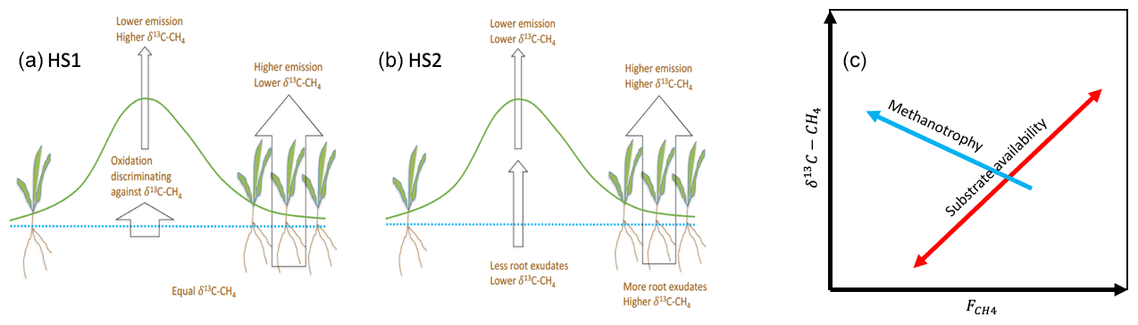
Figure 1 Spatial variation in methane emission based on two hypotheses: (a) HS1, variation is due to methanotrophy, and (b) HS2, variation is due to methanogenesis and the substrate status. Resulting relations between δ¹³C-CH₄ and $F_{{\mathrm{CH}}_{\mathrm{4}}}$ are shown in (c).

In this study, we analyze the observed spatial and temporal variation in CH₄ emission rates from a hemiboreal mire ecosystem and its δ¹³C values to understand the causes of these variations. We aim to shed light on the relative importance of methanogenesis and methanotrophy for the spatial variation in the CH₄ emission rate and the roles of precursor substrate availability and temperature for the seasonal variation in the CH₄ emission rate. We also use taxonomy data to characterize the methanogenic and methanotrophic microbial communities in the mire to reveal the potential of methane production via different pathways as well as microbial methane oxidation.

In order to interpret the variation in CH₄ emission rates and their δ¹³C values, we have formulated a conceptual framework with different simplified hypotheses for the causes of the spatial and temporal variations in methane emission rates. From these we have deduced expected relations between CH₄ emission rates and their δ¹³C values that are used to guide the data analysis and interpretation.

2 Conceptual framework

We will consider two commonly observed phenomena in the variation in CH₄ emission rates from mires. First, there is a spatial variation at the microtopographic level, with the lowest emissions from dry hummocks and inundated ponds and highest emissions from wet lawns (e.g., Riutta et al., 2007; Keane et al., 2021). Second, there is a temporal variation at the seasonal scale, which lags the cycle of air and peat surface temperature and gross primary production but follows the temperature of deeper peat (e.g., Rinne et al., 2018; Chang et al., 2020, 2021; Łakomiec et al., 2021).

We can have two simplified hypotheses regarding the processes leading to the small-scale spatial variability in the CH₄ emission rate. In the first hypothesis on spatial variability (HS1), we assume that the production of CH₄ beneath wetter and drier surfaces is equal but that oxidation by methanotrophic organisms in the oxic layers leads to lower emission of CH₄ from the drier surfaces compared to the wetter surfaces (Fig. 1). In the second spatial hypotheses (HS2), we assume that the differences in the CH₄ emission rate ($F_{{\mathrm{CH}}_{\mathrm{4}}}$) between wet and dry surfaces reflect differences in CH₄ production due to differences in the substrate availability for methanogenesis. While both hypotheses lead to similar differences in the CH₄ emission rates between the wetter and drier surfaces, their relations to the δ¹³C values are different. HS1 would lead to negative correlation between CH₄ emission rate and the δ¹³C value of emitted CH₄ because enzymatic reactions associated with methanotroph metabolism consume preferentially ¹²CH₄, resulting in ¹³C enrichment of residual CH₄. HS2, on the other hand, would lead to positive correlation between the CH₄ emission rate and its δ¹³C value because CH₄ production in conditions with better substrate availability, typically associated with higher methane emission rates of more productive mires, leads to CH₄ with a higher δ¹³C value than with lower substrate availability (Chanton et al., 2005). The better substrate availability can be associated with acetate availability for acetoclastic methanogenesis or better energetics for hydrogenotrophic methanogenesis (Penning et al., 2005; Hornibrook, 2009). Thus, the two hypotheses lead to distinctly different predictions about the relationship between the CH₄ emission rate and its δ¹³C value (Hornibrook, 2009). As a zero hypothesis (HS0) we may have, e.g., a mixture of the abovementioned processes contributing to the spatial variability in CH₄ emission. In this case we may observe no systematic co-variation between the CH₄ emission rate and δ¹³C values.

For the seasonal variation in the CH₄ emission rate, we can hypothesize either that the variation is due to the seasonal development of temperature or that it is modified heavily by the availability of substrates for methanogenesis (Chang et al., 2020, 2021). In the first hypothesis on the temporal variation (HT1), we assume that the temporal variation is due to the seasonal change in peat temperature. As this does not change the δ¹³C value of emitted CH₄, there will be no temporal correlation between the CH₄ emission rate and its δ¹³C value (Fig. 2). In the second temporal hypothesis (HT2) we assume that the seasonal cycle of the CH₄ emission rate is due to the changes in substrate availability. This may be via changes in availability of H₂ for hydrogenotrophic methanogenesis or in availability of acetate for acetoclastic methanogenesis. Thus, the changes in substrate availability may or may not include changes in the methanogenetic pathway. HT2 would lead to positive correlation between the CH₄ emission rate and its δ¹³C value. In the third temporal hypothesis (HT3) we assume that there are significant time lags between the seasonal cycles of the drivers of the CH₄ emission rate, i.e., temperature and substrate availability, which lead to hysteresis-like behavior in the relationship between the CH₄ emission rate and its δ¹³C value.

3 Methods

3.1 Study site and ancillary measurements

We conducted the measurements at Mycklemossen mire (58^∘21^′ N, 12^∘10^′ E; 80 m a.s.l.; Fig. 3) in southwestern Sweden in 2019 and 2020. The site is a part of the SITES¹ Skogaryd research catchment and a candidate to be a class-2 ecosystem site within the ICOS² research infrastructure (J. Heiskanen et al., 2021). Mycklemossen mire lies within the hemiboreal forest zone. The annual 30-year average air temperature from a nearby weather station is 6.8 ^∘C (1981–2010, SMHI Vänersborg), and annual precipitation is 800–1000 mm (1981–2010, SMHI Vänersborg and Uddevalla). The mire is a poor fen with bog characteristics in its vegetation and a pH of 3.9–4.0 (Rinne et al., 2020).

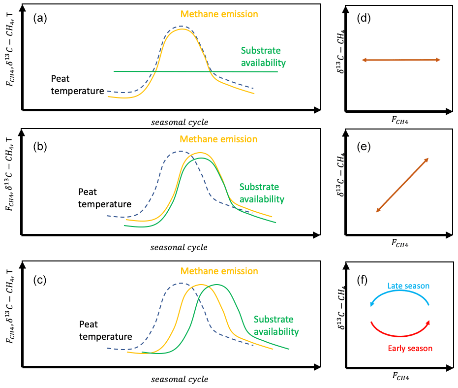
Figure 2 Seasonal variation in methane emission with hypotheses on controlling processes (a HT1; b HT2; c HT3) and resulting relations between δ¹³C-CH₄ and $F_{{\mathrm{CH}}_{\mathrm{4}}}$ (d–f).

A range of meteorological and hydrological parameters are available from the Mycklemossen research site, including air temperature, peat temperature at different depths at four locations, and water table position at three locations.

3.2 CH₄ emission and δ¹³C measurements

We used two approaches to measure the δ¹³C value of the emitted CH₄, the automated static chamber approach (e.g., McCalley et al., 2014) and the nocturnal boundary-layer accumulation (NBLA) approach (e.g., Sriskantharajah et al., 2012). With the former we obtain the CH₄ emission rate and its δ¹³C value resolved at the microtopographic scale, while with the latter we obtain an average δ¹³C value of the emitted CH₄ over a larger area of the mire.

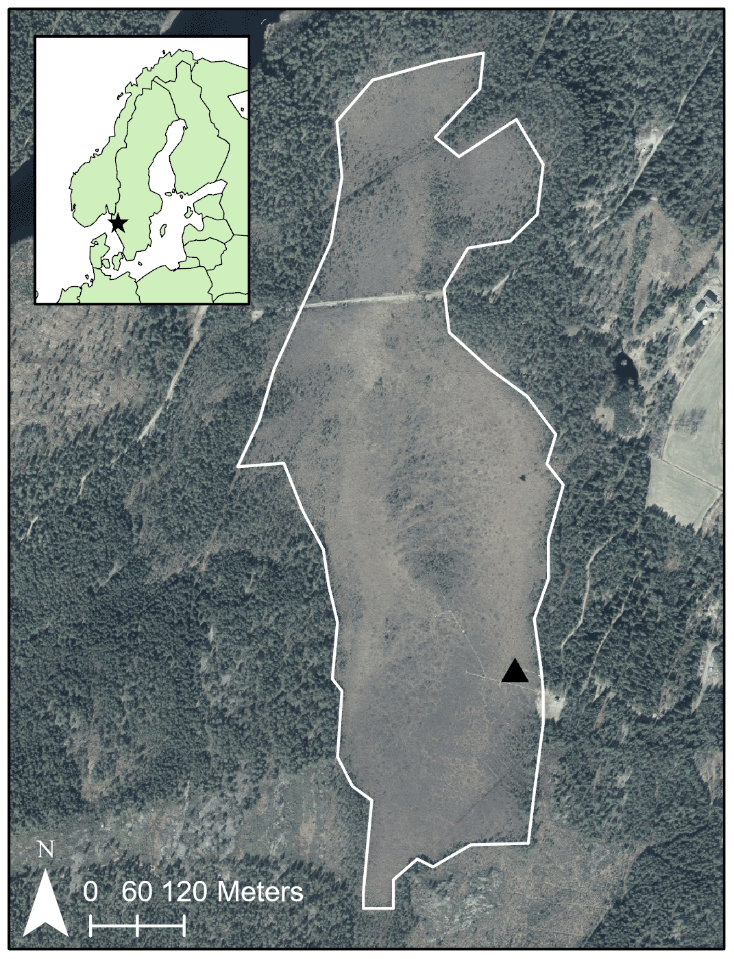
Figure 3 Map of Mycklemossen (outlined in white). The black star indicates the location of Mycklemossen within Scandinavia; the black triangle indicates the location of the chamber and NBLA measurements. Data sources: © Lantmäteriet, © EuroGeographics.

For the chamber approach, we used six automated chambers with dimensions of $\mathrm{44.5}\times \mathrm{44.5}\times \mathrm{40.5}$ cm. In addition, the frame onto which the collar is placed introduces additional volume as it is approximately 5 cm high from the peat surface. This volume is more challenging to determine accurately due to the uneven peat surface. The chambers were transparent, made out of polymethyl methacrylate, and equipped with a lid that opened and closed automatically. Each chamber was equipped with a fan to ensure sufficient mixing of air in the chamber headspace, a soil thermometer (probe 107, Campbell Scientific, Inc., UT, USA), a photosynthetic photon flux density (PPFD) sensor (SQ-500, Apogee Instruments, Inc., UT, USA) situated inside the chamber, and a vent tube to prevent pressure changes when opening and closing the lid. Each chamber cycle was 30 min and started with 5 min where the chamber and the tubing to and from the gas analyzer were ventilated. The chamber lid then closed for 25 min. The long closure time was needed to ensure a robust fit using the Keeling plot approach (Keeling, 1958). All measurements of the methane mixing ratios and δ¹³C were performed using a Picarro G2201-i cavity ring-down spectroscopic (CRDS) analyzer (Picarro, Inc., CA, USA). The chamber measurements were conducted between 07:00–19:00 CEST (central European summer time), resulting in four measurements from each chamber every day. The time between 19:00 and 07:00 CEST was used for measurements with the NBLA approach.

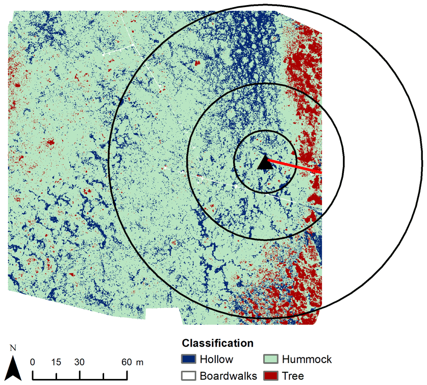
Figure 4 Distribution of dry and wet areas in Mycklemossen according to microtopography. The black triangle indicates the sampling location of measurements used for the nocturnal boundary-layer accumulation (NBLA) approach. The chambers were situated along the boardwalk (red line). Black circles indicate the distances (20, 50, 100 m) from the NBLA sampling point.

Table 1 Dominant vegetation in flux chambers. D: dominant; P: present. Niche indicates the niche of the species. The relative elevation (above 80 m a.s.l.) of the moss surface at each chamber (CH_1 to CH_6) is indicated.

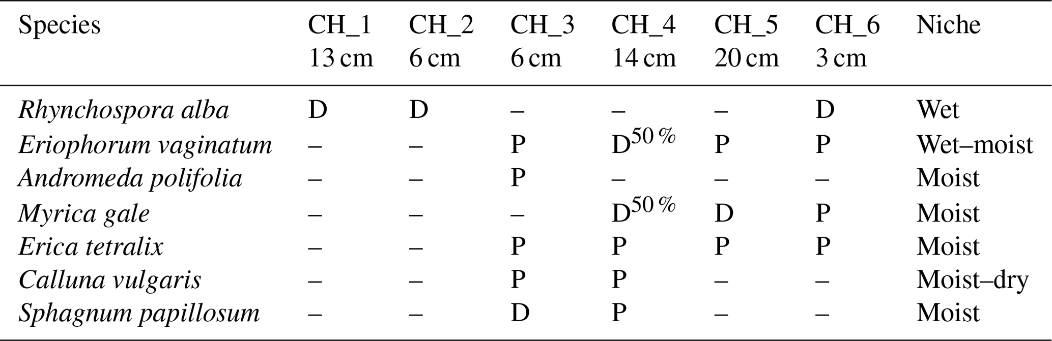
The chambers were placed along a boardwalk (Fig. 4). The topography of the mire is not very pronounced with the maximum difference in surface height between chamber locations being 17 cm. Furthermore, the relative elevations were not indicative of the dominant vegetation in the chambers (Table 1, Fig. 5). The vegetation in the chambers falls into three categories. In chambers 1 and 2 there is a major presence of aerenchymatous sedges, typical of moist conditions in the mire. Chamber 3 is dominated by Sphagnum mosses, also common in moist conditions. In chambers 4 and 5 there is a considerable presence of woody shrubs, typical of drier conditions. The vegetation in chamber 6 is intermediate between sedge-dominated and shrub-dominated.

The emission rate of CH₄ was calculated as the linear fit of the CH₄ mixing ratio to time during the first 4 min of the closure. The first 60 s was discarded to avoid the disturbances at lid closure, leaving 3 min of data for the linear fitting. For data quality assurance R² and root-mean-square error (RMSE) were calculated for each chamber closure. Processing and analysis of stable isotope data were conducted with MATLAB (R2015b).

The δ¹³C of the emitted CH₄ was obtained by the Keeling plot approach (Keeling, 1958). In this approach, we plotted the measured δ¹³C against the inverse of the CH₄ mixing ratio (χ). The δ¹³C of the emitted methane was then obtained as the intercept of the δ¹³C value at 1/χ=0, by fitting a line,

$$\begin{array}{}\text{(1)}& {\mathit{\delta }}^{\mathrm{13}}\mathrm{C}\left(\mathit{\chi }\right)=a+b{\mathit{\chi }}^{-\mathrm{1}},\end{array}$$

to the data. Here δ¹³C(χ) is the observed δ¹³C value of CH₄ in the chamber air at the methane mixing ratio of χ and a and b are coefficients obtained by line fitting. Coefficient a is the intercept, which will give us the isotopic signature (δ¹³C value) of the emitted methane. The confidence interval of the δ¹³C at the intercept was obtained by the function linfitxy in MATLAB (Browaeys, 2021). We removed the data from closures where the uncertainty in δ¹³C of emitted CH₄ was larger than 20 ‰.

For the NBLA approach we measured the CH₄ mixing ratio and δ¹³C at 0.4 m above the mire surface during the nighttime. As the emitted CH₄ is accumulated in the shallow stable nocturnal surface layer, we can employ a similar two-end-member mixing model to that for the chamber measurements (Rinne et al., 2021). Thus, we obtain the δ¹³C of the emitted CH₄ by the Keeling plot approach (Eq. 1).

In addition to the automated measurements, we occasionally took manual air samples from chambers during closures and analyzed these with an isotope ratio mass spectrometer for comparison with the automated measurements. From each chamber closure, eight samples were taken into 2 L Supel™-Inert foil gas sampling bags (Sigma-Aldrich, Merck, MA, USA). The eight samples from each chamber were divided into two sets, one transported to Utrecht University and the other one to Royal Holloway, University of London, for analysis. The analysis methods are described by Röckmann et al. (2016) and Fisher et al. (2006). These results were compared with CRDS results, and the difference in the resulting δ¹³C-CH₄ values of 3.4 ‰ was added to the δ¹³C-CH₄ values calculated using the CRDS data.

In order to reduce measurement noise, especially in the δ¹³C values, we aggregated the calculated CH₄ emissions and their δ¹³C values to 10 d averages. To analyze the spatial variability, we plotted the δ¹³C values against CH₄ emission rates during each 10 d interval. For the analysis of temporal variation, we plotted the δ¹³C values against the CH₄ emission rates from each chamber.

3.3 Upscaling the δ¹³C estimates

To scale up the δ¹³C values obtained from the different surface types by the chamber method to the isotopic signature of the whole mire, δ¹³C_mire, we weighted the δ¹³C values of different surface types by the areal contribution of these surface types and by their CH₄ emission rates:

$$\begin{array}{}\text{(2)}& {\mathit{\delta }}^{\mathrm{13}}{\text{C}}_{\text{mire}}=\left(\sum {\mathit{\delta }}^{\mathrm{13}}{\text{C}}_i{f}_i{F}_i\right){\left(\sum f_i{F}_i\right)}^{-\mathrm{1}},\end{array}$$

where δ¹³C_i is the isotopic signature of the CH₄ emission from the surface type i, f_i is fraction of the mire covered by surface type i, and F_i is the CH₄ emission rate of the surface type i. Both δ¹³C_i and F_i are based on the chamber measurements.

Figure 5 (a) Photo showing the relative location of chambers along the boardwalk. (b) Photos of vegetation inside each chamber, numbered 1–6. NBL indicates the inlet for measurement of ambient air for the nocturnal boundary-layer accumulation approach.

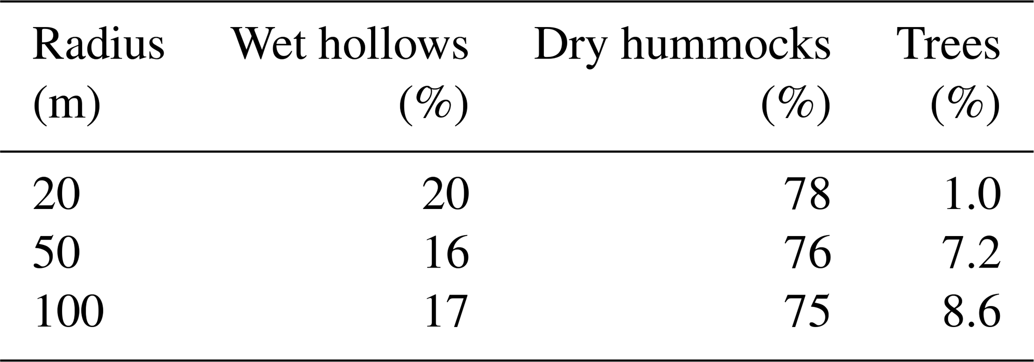
The map of mire surface types used to determine f_i in Eq. (2) was based on RGB and multispectral images collected with an unmanned aerial vehicle (UAV) in 2017. A random forest classifier (Breiman, 2001) was used to divide the mire into three vegetation classes – hummocks, hollows, and trees – producing a total accuracy of 81 % (see Fig. 4 and Kelly et al., 2021, for more details). Table 2 shows the proportion of each surface type for different radii around the NBLA tower. In the upscaling, average the δ¹³C and CH₄ emission rate from chambers 1 and 2 represented the values of wet hollows, while average values from chambers 4–6 represented those from drier hummocks. As there were very few data from chamber 3, especially in 2020, we did not use chamber 3 for upscaling. The hollows were given areal coverage of 20 % and hummocks 80 %.

Table 2 Proportions of different vegetation types in different radii around the NBLA tower.

3.4 Genomic analysis

Peat material for genomic analysis was collected in 2018 from three different surface types specified through the wetness classification (n=17). Using a 1.5 m long box corer, peat material was cut from the oxic–anoxic interface (∼5 cm) and the anoxic zone (∼30 cm). The peat material was immediately frozen using liquid nitrogen and stored in a −80 ^∘C freezer prior to beginning genetic DNA (gDNA) extraction. The gDNA was extracted from 0.25 mg of peat following the DNeasy^® PowerSoil^® kit manufacturer's protocol (Qiagen, Hilden, Germany).

The extracted gDNA was hybridized to a set of custom-designed oligonucleotide probes which enrich the gene sequences related to CH₄ metabolism. This was achieved using the “captured metagenomics” method. Briefly, genes encoding enzymes related to the CH₄ production and consumption were identified in the Kyoto Encyclopedia of Genes and Genomes (KEGG) database (Kanehisa et al., 2015) and were downloaded via a custom R script (https://github.com/dagahren/metagenomic-project, last access: 17 August 2022). The target sequences downloaded from KEGG were used to design custom hybridization-based probes for sequence capture based on the MetCap pipeline (Kushwaha et al., 2015). For further details on probe design, library construction, and sequencing, refer to White et al. (2022).

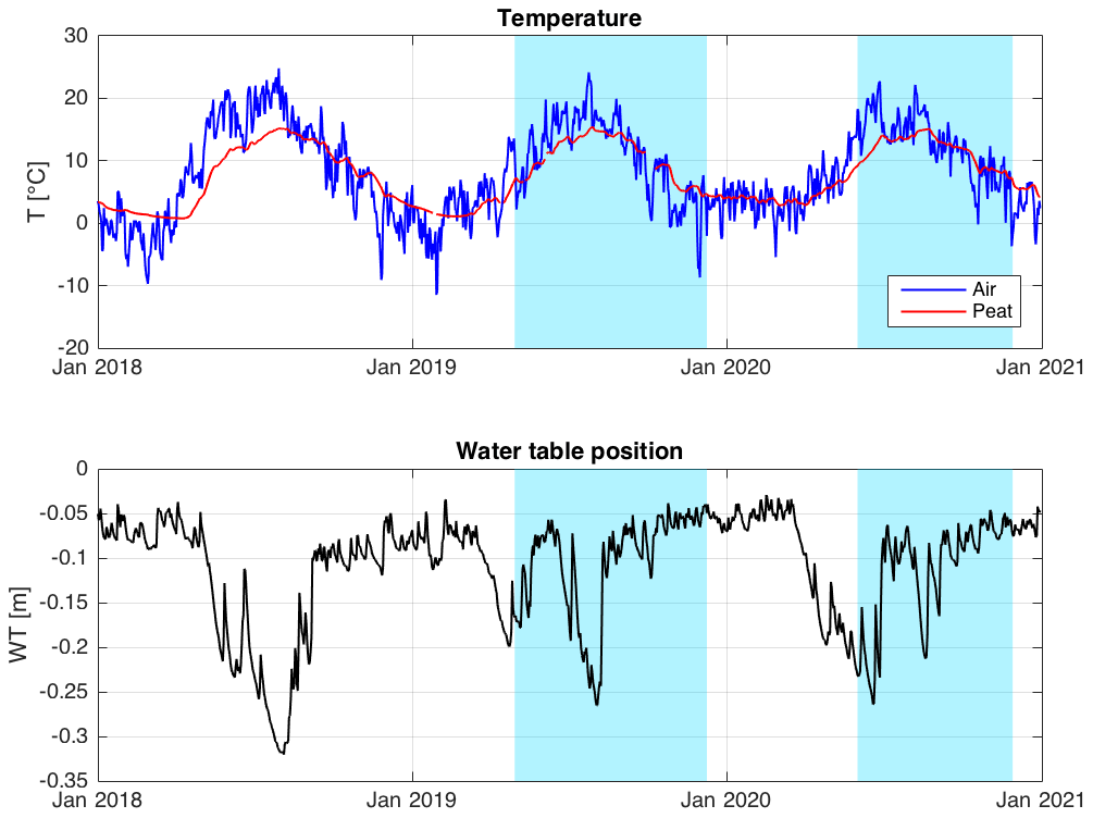
Figure 6 Meteorological conditions during 2018–2020. Periods of δ¹³C-CH₄ and $F_{{\mathrm{CH}}_{\mathrm{4}}}$ measurements are indicated by blue shading.

Libraries were multiplexed in pools of 15 in equimolar amounts based on the concentrations and sizes of samples. A total of 1 µg of each pool was transferred to a capture tube where target gDNA was hybridized to the custom probes according to the NimbleGen SeqCap EZ Library SR User's Guide (Version 4.3, October 2014). The captured libraries were sequenced on an Illumina HiSeq 4000 platform using sequencing by synthesis technology to generate 2×150 base pair paired-end reads.

Following sequencing, raw .fastq files were trimmed for the presence of Illumina adapter sequences using Cutadapt version 1.2.1 (Martin, 2011). The reads were further trimmed using Sickle version 1.200 with a minimum window quality score of 20 (Joshi, 2011). The sequence reads from each of the captured data set were submitted to MG-RAST, an online metagenomics annotation program using default parameters (Meyer et al., 2008). The taxonomic abundances were annotated using the RefSeq database (O'Leary et al., 2016). Following annotation, taxa were filtered for off-target sequences, leaving only abundances of methanogenic and methanotroph microbial communities using the built-in taxonomic filter within the MG-RAST analysis page.

The relative abundance of methanogens and methanotrophs was calculated via the phyloseq package v1.3.0 (McMurdie and Holmes, 2013). To allow for the small sample size and uneven distribution of replicates, a PERMANOVA (permutational multivariate analysis of variance) was used with 999 permutations (Anderson, 2001) to identify significant differences between categories. Following square root transformation, we calculated ordination using Bray–Curtis distances, and finally, a Wilcoxon pairwise post hoc test was used to identify significant differences between the different wetness categories via the vegan package v 2.5 (Oksanen et al., 2019). All genetic analysis was completed in R statistics package v 3.6.1 (R Core Team, 2018) and visualized using the ggplot2 package v 3.3.2 (Villanueva and Chen, 2019).

4 Results

4.1 Climate

The average daily air temperatures at the mire range from slightly below zero to above 20 ^∘C (Fig. 6). The water table is typically drawn down during early summer before being replenished by late summer and autumn rains (Fig. 6). In 2018, the mire was affected by a severe heat wave and drought, as shown by the long duration of the water table drawdown, as well as by the high air temperatures that summer. The years 2019 and 2020, during which the measurements reported here were conducted, were closer to average conditions.

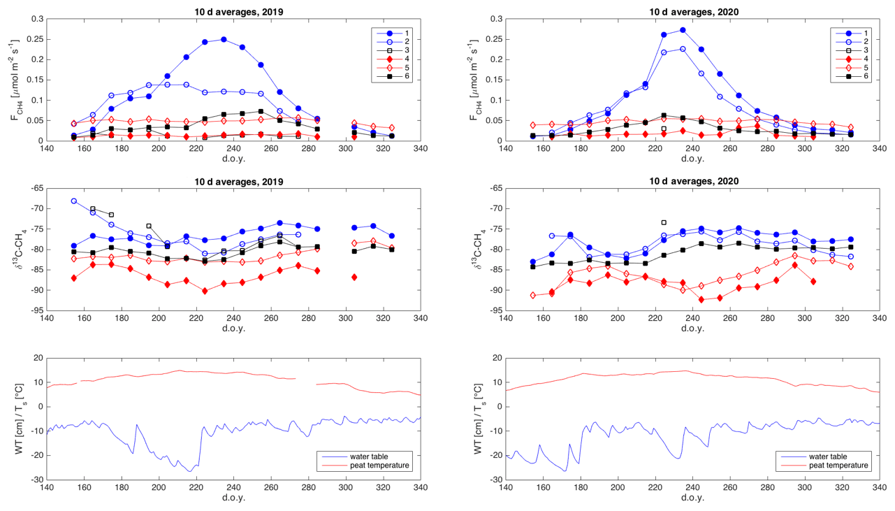
Figure 7 Time series of 10 d averages of methane emission and δ¹³C-CH₄ measured from the six chambers and peat temperature at 30 cm depth and the water table position in 2019 and 2020.

4.2 CH₄ emission rates and δ¹³C values

The time series of CH₄ emission rates from most chamber locations shows a typical seasonal cycle of CH₄ emission, with the highest emission rates in late summer (Figs. 7, S1 in the Supplement). We see also distinct differences between the emission rates from different chambers, indicating strong small-scale spatial variation in the CH₄ emission rate. The highest emission rates are observed from chambers 1 and 2, with abundant aerenchymatous sedges. Chambers 3 and 4 have very low CH₄ emission rates, despite differences in vegetation, while chambers 5 and 6 have intermediate emission rates. The emission rate from chamber 5 has a less pronounced annual cycle than from the other chambers.

The δ¹³C values of emitted CH₄ also show relatively large differences depending on the chamber location (Figs. 7, S2). In general, chamber locations with high emission rates have less depleted (less negative) δ¹³C values of emitted CH₄. The seasonal cycle of the δ¹³C values is much less obvious or systematic than that of the CH₄ emission rate.

Figure 8 (a, b) Examples of spatial variation in 10 d averages of δ¹³C-CH₄ against $F_{{\mathrm{CH}}_{\mathrm{4}}}$, during three 10 d time periods in 2019 and 2020. Chambers: 1, solid circles; 2, open circles; 3: open squares; 4: solid diamonds; 5: open diamonds; 6: solid squares. Colors of markers and lines indicate the period: day of year (doy) 210–219, red; doy 220–229, blue; doy 230–239, black. The solid lines indicate correlation with p<0.01 and the dashed line with p<0.05. (c) R² between 10 d averages of δ¹³C and $F_{{\mathrm{CH}}_{\mathrm{4}}}$, without chamber 3. (d) p value of correlation, without chamber 3.

The δ¹³C values and CH₄ emission rates generally show a positive spatial relationship during many of the 10 d periods (Figs. 8 and A1 and A2 in the Appendix). The positive relationship was more pronounced during the period of high emission rates (day of year (doy) 200–260) and more evident in 2019 than in 2020. However, chamber 3 deviated consistently during 2019 from the general behavior of the other chambers. Unfortunately, there were hardly any data that passed the quality assurance and control criteria from that chamber during 2020 due to low CH₄ emission rates. Omitting the data from chamber 3 led to statistically significant correlations between the CH₄ emission rate and its δ¹³C value during many of the 10 d periods (Fig. 8).

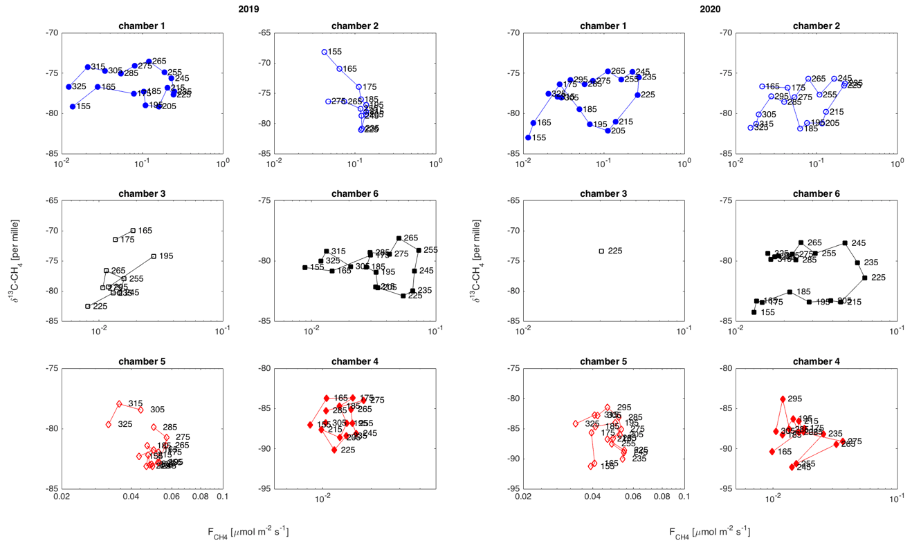
Figure 9 Temporal variation in δ¹³C-CH₄ against $F_{{\mathrm{CH}}_{\mathrm{4}}}$, in each chamber location in 2019 and 2020. The marker labels indicate the day of year. Only very few data points from chamber 3 passed the quality criteria in 2020, resulting in only one 10 d average.

The temporal relation of δ¹³C values and CH₄ emission rates showed a hysteresis-like behavior at three of the measurement locations (chambers 1, 2, and 6) during 2020 and at two locations (chambers 1 and 6) in 2019 (Fig. 9). These locations are either wet or intermediate sites with relatively high emission rates. In these locations, the δ¹³C values of emitted CH₄ were lower in the early part of the growing season than during a period with similar emission rates later in the season. The dry sites with lower CH₄ emission did not show observable systematic behavior in their δ¹³C–$F_{{\mathrm{CH}}_{\mathrm{4}}}$ relation.

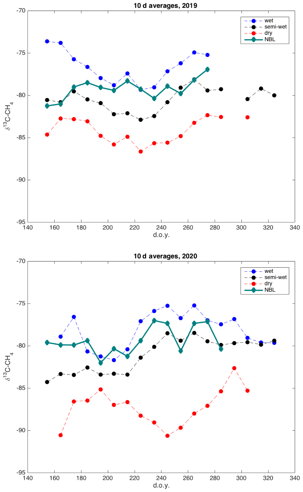
Figure 10 Time series of 10 d average δ¹³C-CH₄ derived by nocturnal boundary-layer Keeling plot approach (green) and averages of wet (blue), intermediate (black), and dry (red) locations, for 2019 and 2020.

The δ¹³C values of emitted CH₄ derived by the nocturnal boundary-layer method are in the same range as the δ¹³C values observed at the wet and intermediate chambers, with some similarities in their seasonal cycle (Figs. 10, S3). The upscaling of the chamber data using the microtopographic map resulted in an average δ¹³C value of emitted CH₄ of −81.3 ‰. The average δ¹³C value of emitted CH₄ according to NBLA measurements was −79.3 ‰.

4.3 Genomic analysis

In total, 20 methanogens and 5 methanotrophs were identified at the genus level. Genera were spread across four classes of methanogens including Methanobacteria, Methanococci, Methanomicrobia, and Methanopyri. In addition, three classes of methanotrophs including type-I Gammaproteobacteria, type-II Alphaproteobacteria, and Verrucomicrobia were also detected. These genera included methanogens with the ability to perform methanogenesis via all metabolic pathways including hydrogenotrophic, acetoclastic, and methylotrophic and the specialist methanogen Methanosarcina (Hydr/Methyl/Aceto – hydrogenotrophic, methylotrophic, and acetoclastic – methanogen), which holds the ability to metabolize via multiple alternative pathways.

The proportion of methanogens to methanotrophs is a 58 % to 42 % split when combining all the samples. The dominant methanogens were hydrogenotrophic methanogens (46 %), followed by the multiple metabolic pathway genus Methanosarcina (10 %), with the methylotrophic and acetoclastic methanogens contributing 2 % and ≤1 %, respectively. The dominant methanotrophs were the type-II Alphaproteobacteria (30 %), followed by type-I Gammaproteobacteria (8 %) and Verrucomicrobia (4 %).

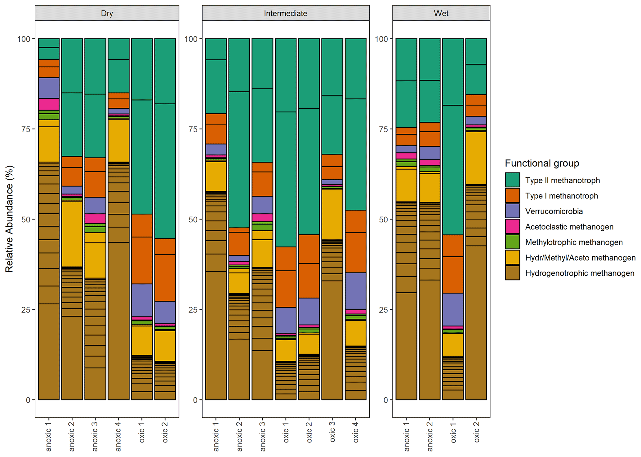
Figure 11 Taxonomic composition: the relative abundance (%) of methanogenic and methanotrophic microbes at the genus level. Color indicates the functional group and which metabolic pathway is utilized during metabolism.

Significant variation in the relative abundance of taxa was observed between the wet, intermediate, and dry categories (p≤0.02) (Fig. 11). The PERMANOVA indicated that 37 % of the variation in taxa was explained by the wetness category (R²=0.37, p≤0.02). When testing pairwise between categories, significant differences in the relative abundance of taxa occurred between wet–dry (p≤0.04) and wet–intermediate categories (p≤0.04) but not between the dry–intermediate categories (p≥0.05).

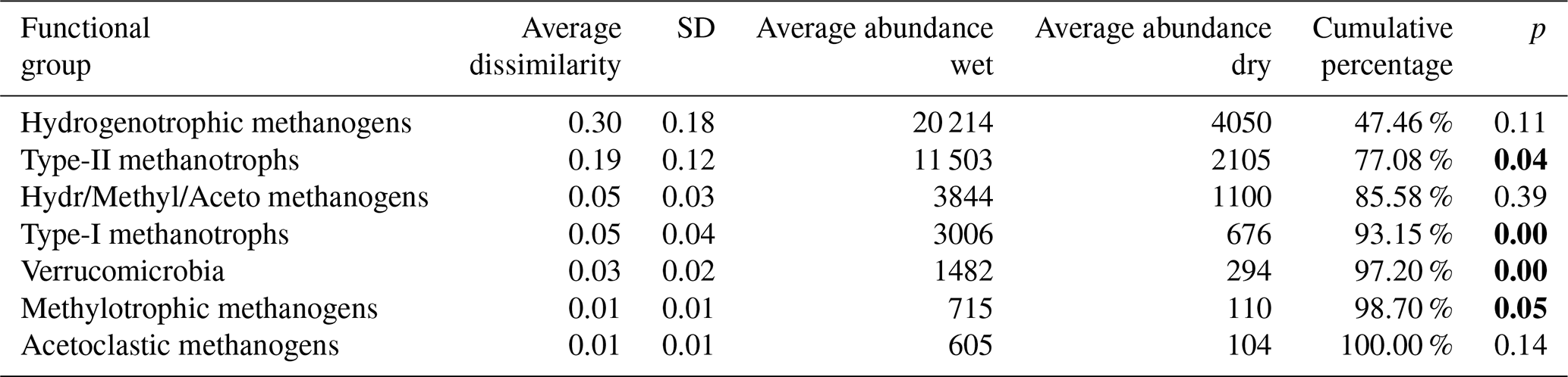
Table 3 Results of SIMPER (similarity of percentage, a function that performs pairwise comparisons of groups of sampling units and finds the average contributions of each species to the average overall Bray–Curtis dissimilarity) analysis between intermediate (n=7) and wet (n=4) plots. Functional groups are ranked according to their average contribution to dissimilarity between plots. Standard deviation (SD), average abundances, percentage of cumulative contribution, and the permutation p value (probability of obtaining a larger or equal average contribution in random permutation of the group factor) are also included.

p values below 0.05 are in bold.

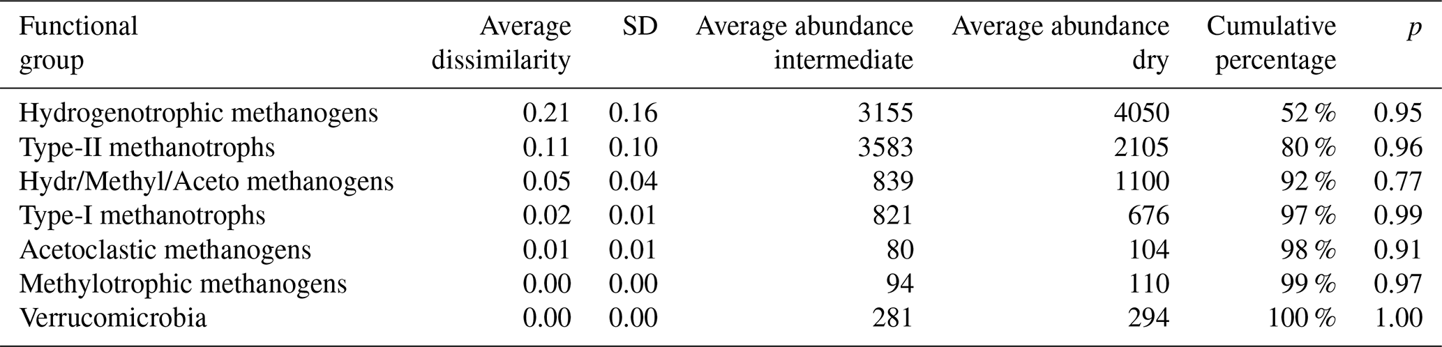
The functional group contributing the most to dissimilarity in all comparisons was the hydrogenotrophic methanogens, with an average dissimilarity of 0.29±0.19 SD between intermediate–wet, 0.20±0.16 SD between intermediate–dry, and finally 0.30±0.17 SD between wet–dry categories (Tables 3, 4, 5). Although contributing the most to dissimilarity, the difference was identified as non-significant when comparing between categories. Type-II methanotrophs, multiple metabolic pathway Methanosarcina, type-I methanotrophs, and hydrogenotrophic methanogens contributed second-, third-, fourth-, and fifth-most to dissimilarity, respectively. Interestingly, methylotrophic methanogens contributed little to dissimilarity but were the only methanogenic functional group to be significantly higher in abundance in wet locations when compared to intermediate (p≤0.027) and dry (p≤0.046) plots. Type-I methanotrophs and Verrucomicrobia methanotrophs had significantly higher average abundance in wet locations when compared to intermediate (p≤0.01) and dry plots (p≤0.004). However, type-II methanotrophs were only significantly higher in abundance in wet plots when compared to dry (p≤0.036).

Table 4 Results of SIMPER analysis between intermediate (n=7) and dry (n=6) plots. Taxa are ranked according to their average contribution to dissimilarity between plots. Standard deviation (SD), average abundances, percentage of cumulative contribution, and the permutation p value (probability of obtaining a larger or equal average contribution in random permutation of the group factor) are also included.

5 Discussion

The CH₄ emitted from surfaces covered by different vegetation types shows large differences in its δ¹³C values. In the late summer of 2020, the differences between the 10 d average δ¹³C values from different chambers were up to 10 ‰–15 ‰. Considering the modest microtopography of Mycklemossen mire and the closeness of the measurement locations (Table 1, Fig. 5), this indicates a considerable small-scale spatial variation in the processes leading to CH₄ emission. Our findings are in line with the large observed differences in CH₄ emission rates due to small-scale spatial variability from other mire ecosystems (e.g., Riutta et al., 2007; Keane et al., 2021). The spatial variation in δ¹³C values observed at Mycklemossen are in the same range as that observed at Abisko-Stordalen mire (68^∘20^′ N, 19^∘30^′ E) in northern Sweden by McCalley et al. (2014). Furthermore, McCalley et al. (2014) and Mondav et al. (2017) identified the same genera of hydrogenotrophic methanogens in Abisko-Stordalen mire as we found at Mycklemossen, with the same genus (Methanoregula) being dominant. The similar range of the δ¹³C values and similar methanogens at Mycklemossen and Abisko-Stordalen mires are interesting as these mires are located over 1100 km apart and differ considerably in their microtopography and climate. The microtopographic height differences at Abisko-Stordalen are about 1 m, as compared to about 20 cm at Mycklemossen. Furthermore, due to the cold climate and thin wintertime snow cover, Abisko-Stordalen features discontinuous permafrost in the form of palsas, whereas Mycklemossen is a hemiboreal non-permafrost mire.

Table 5 Results of SIMPER analysis between wet (n=4) and dry (n=6) plots. Taxa are ranked according to their average contribution to dissimilarity between plots. Standard deviation (SD), average abundances, percentage of cumulative contribution, and the permutation p value (probability of obtaining a larger or equal average contribution in random permutation of the group factor) are also included.

p values below 0.05 are in bold.

The spatial variation in the δ¹³C values of emitted CH₄ is systematic over the growing season and 2 years of measurements. Generally, the wet sedge-dominated plots with higher emission rates are associated with higher δ¹³C values and the dry shrub-dominated plots with lower emission rates with lower δ¹³C values, indicating the likely importance of substrate availability and methanogenesis in determining the spatial variation in the CH₄ emission rate. Similar spatial relations between δ¹³C and the CH₄ emission rate have been observed by, e.g., Hornibrook and Bowes (2007) in Welsh mires and McCalley et al. (2014) in the Swedish subarctic Abisko-Stordalen mire. However, the position of chamber 3 in the δ¹³C–$F_{{\mathrm{CH}}_{\mathrm{4}}}$ emission rate diagram (Figs. 8, A1, A2) suggests an effect of methanotrophy on CH₄ emission and its δ¹³C value from this location. This may be due to the dominance of Sphagnum mosses in this chamber, which have been shown to support considerable methanotrophy (Larmola et al., 2010). The significantly higher abundance of type-II methanotrophs in wetter locations as compared to dry and intermediate supports this suggestion.

Of our two hypotheses on the origins of the spatial variation in CH₄ emission rates, one (HS1) assumes methanotrophy to be the key explanatory process while the other (HS2) assumes substrate availability to drive the spatial variation. The relation between the CH₄ emission rate and δ¹³C values of emitted CH₄ we observed, especially at locations with vascular vegetation cover, mostly corroborates the latter hypothesis (HS2). Corroboration of the HS1 hypothesis would have required a negative correlation between the δ¹³C and CH₄ emission rate. Furthermore, the presence of hydrogenotrophic, acetoclastic, and methylotrophic methanogens enables the community to utilize all substrates available. Thus, it is unlikely that methanotrophy plays a major role in explaining the spatial variation in CH₄ emission from this mire system, especially as the moss-dominated areas seem to cover a minor area of the mire.

As it is possible that there are seasonal differences in the factors affecting the spatial variability in the methane emission (temperature, substrate availability, methanotrophy), we analyzed the spatial variation throughout the growing seasons as 10 d averages. According to the observed spatial relations between δ¹³C and CH₄ emission rates during these two growing seasons, there were no major temporal shifts in the behavior of the δ¹³C–$F_{{\mathrm{CH}}_{\mathrm{4}}}$ relationship (Figs. A1 and A2). The δ¹³C values and CH₄ emission rate, omitting chamber 3, showed a tendency toward positive correlation for most of the growing seasons. Thus, it seems that the processes leading to the spatial variations in CH₄ emission are similar throughout the growing season.

The temporal variation in δ¹³C was smaller and less systematic than its spatial variation. Interestingly, this temporal relation does not show similar systematic behavior to the spatial variation, indicating that the space-for-time analogy may not be valid on these seasonal timescales. The temporal behavior of δ¹³C in relation to the CH₄ emission rate shows a hysteresis-like behavior at some of the chamber plots. The hysteresis-like behavior is clear in wet or intermediate plots with high emission rates. The lack of observable hysteresis-like behavior in the other plots could be due to the small range of emission rates, leading to random variation in the data to mask any systematic behavior. The hysteresis-like behavior indicates that the temporal variation in CH₄ emission rates from this mire could be a result of two time-lagged compounding effects, following the HT3 hypothesis, especially as the variation in the δ¹³C value and CH₄ emission rate on the mire scale is mostly affected by the high-emitting surfaces. The increasing CH₄ emissions during the first half of the growing season could be caused by increasing peat temperature enhancing the activity of methanogenic Archaea (Juottonen et al., 2008). Later in the growing season, the increased input of root exudates from vascular plants would increase the substrate availability, resulting in higher δ¹³C values than in the early season yet similar CH₄ emission rates. However, we cannot assign the whole seasonal cycle of CH₄ emission rates to changes in substrate availability as this would result in a pronounced positive relationship between δ¹³C and CH₄ emission rates, which we did not observe. According to the genetic analysis, the microbial community holds the functional potential to produce CH₄ via the hydrogenotrophic and acetoclastic pathways, thus enabling shifts in δ¹³C following the seasonal changes in availability of substrate. However, the highly depleted δ¹³C, mostly between −90 ‰ and −70 ‰, does indicate dominance of hydrogenotrophic methane production at this mire, as the hydrogenotrophic pathway produces CH₄ with δ¹³C below 60 ‰, while an acetoclastic pathway would result in CH₄ with δ¹³C above −60 ‰ (Whiticar, 1999; McCalley et al., 2014). Therefore the changes in δ¹³C of emitted CH₄ are most likely due to energetics of the hydrogenotrophic methanogenesis (Penning et al., 2005; Hornibrook, 2009). The hysteresis between temperature and CH₄ emission, as observed by Chang et al. (2020, 2021) and Łakomiec et al. (2021), could be partly due to the seasonal development of peat temperature and partly due to the changes in substrate availability for methane production.

The δ¹³C values of emitted CH₄ derived by the nocturnal boundary-layer accumulation (NBLA) approach corresponded in magnitude to the values of the wet and intermediate surfaces. As these surfaces dominate the emission, it is natural that the NBLA approach will correspond to these more closely than to the dry surfaces with low CH₄ emission. The upscaled δ¹³C from the chamber measurements was in a similar range to the mire-scale δ¹³C measured by the NBLA method, indicating the dominance of hydrogenotrophic methanogenetic pathways. Obtaining reliable mire-scale isotopic signatures is crucial, for example for the use of isotopic data for source apportioning of CH₄ by atmospheric inversions. Here we show that the chamber δ¹³C measurements can be successfully upscaled using a mire surface characterization based on UAV data. Such an approach enables the calculation of mire-scale δ¹³C estimates at sites where NBLA measurements are not available. In combination with UAV-upscaled CO₂ fluxes (e.g., Kelly et al., 2021), there are further opportunities to examine the impacts of spatial variations in vegetation productivity and respiration on CH₄ emission rates and δ¹³C values.

The mire-scale δ¹³C value of emitted CH₄ observed at Mycklemossen (−81 ‰ to −79 ‰) is somewhat lower than observations in northern Scandinavia by Fischer et al. (2017) and at the lower end of the wetland δ¹³C-CH₄ distribution as presented by Menoud et al. (2022). All these show considerably lower δ¹³C values of CH₄ emitted from northern mire ecosystems than the average δ¹³C values for wetland CH₄ emissions used in many atmospheric inversion studies (−60 ‰ to −58 ‰; Mikaloff-Fletcher et al., 2004a, b; Bousquet et al., 2006; Monteil et al., 2011). Together with the wider data sets of Fisher et al. (2017) and Menoud et al. (2022), the observations presented here would support using a lower δ¹³C value for CH₄ emitted from northern mire ecosystems in atmospheric inversion studies.

6 Conclusions

We conducted automatic chamber and nocturnal boundary-layer accumulation (NBLA) measurements of δ¹³C values of emitted CH₄, as well as genomic analyses of the CH₄-relevant microbial communities, to investigate the drivers of the spatial and temporal variability in the CH₄ emission rate and δ¹³C value in a hemiboreal Swedish mire. Despite the small elevation differences (<20 cm) between the microtopographic zones in the mire, we observed stark contrasts in the CH₄ emission rates and δ¹³C values between the zones, similar in magnitude to mires which have much more pronounced microtopography. According to the relationships between δ¹³C values and CH₄ emission rates we observed, the spatial variability in CH₄ emission from Mycklemossen mire is unlikely to be controlled mostly by methanotrophy. Instead, variations in methanogenesis due to the differences in substrate availability, following our hypothesis 2 on spatial variability (HS2), seem to be a more likely source of most of the variation in CH₄ emission rates. The seasonal variation in CH₄ emission is likely controlled by both temperature and substrate availability, leading to hysteresis-like behavior in the δ¹³C–$F_{{\mathrm{CH}}_{\mathrm{4}}}$ relationship, following our hypothesis 3 on temporal variability (HT3). The taxonomic data show the functional potential to produce CH₄ via multiple metabolic pathways, enabling shifts following changes in the substrate availability. However, the highly depleted δ¹³C values observed indicate the dominance of hydrogenotrophic methanogenesis, and thus the variation in δ¹³C may be due to the energetics of this process. Interestingly, the measurement plot with Sphagnum-dominated vegetation diverged from the general spatial δ¹³C–$F_{{\mathrm{CH}}_{\mathrm{4}}}$ relation, warranting future studies on this vegetation type. In addition, we confirmed that drone-based upscaling of δ¹³C chamber measurements provides reliable mire-scale estimates when compared to NBLA δ¹³C estimates. The observed mire-scale δ¹³C values were at the lower end of reported δ¹³C values from northern mires and, together with these, support the need for revising the δ¹³C value for northern wetland systems used in atmospheric inversion studies. The results obtained can help to constrain our theories on the causes of the variability in methane emission from mire ecosystems and can thus be useful in development of numerical models of mire biogeochemistry, needed to predict the fate of northern mire ecosystems in the changing climate.

Appendix A: Spatial δ¹³C-CH₄–$F_{{\mathrm{CH}}_{\mathrm{4}}}$ relations as 10 d averages

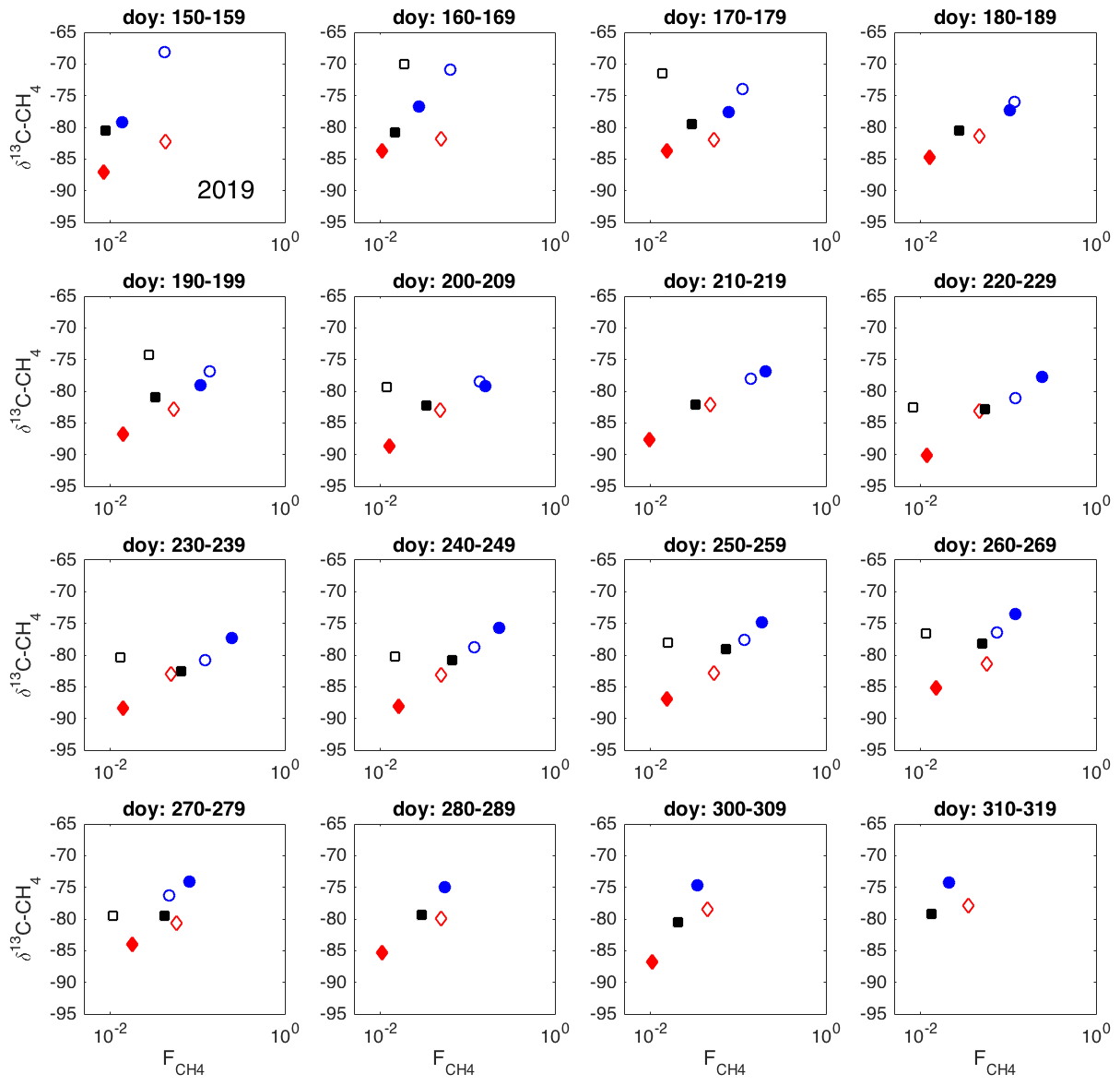
Figure A1 Spatial variation in δ¹³C-CH₄ against $F_{{\mathrm{CH}}_{\mathrm{4}}}$, as 10 d averages during 2019. Chamber 1: solid blue circle; chamber 2: open blue circle; chamber 3: open black square; chamber 4: solid red diamond; chamber 5: open red square; chamber 6: solid black square.

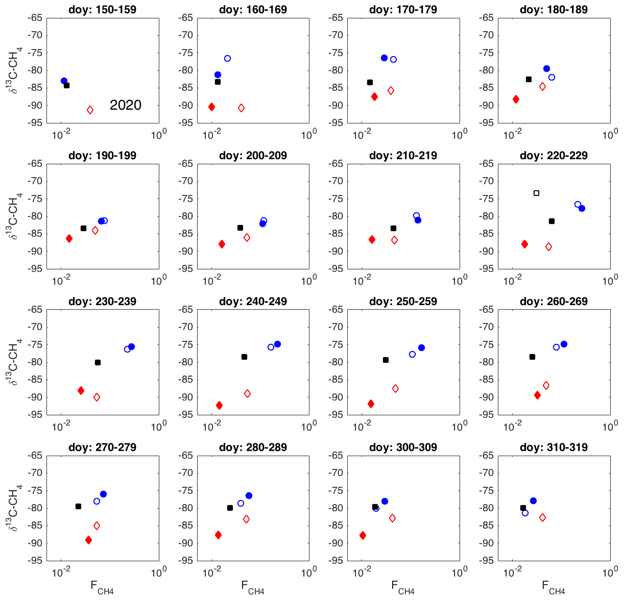
Figure A2 Spatial variation in δ¹³C-CH₄ against $F_{{\mathrm{CH}}_{\mathrm{4}}}$, as 10 d averages during 2020. Chamber 1: solid blue circle; chamber 2: open blue circle; chamber 3: open black square; chamber 4: solid red diamond; chamber 5: open red square; chamber 6: solid black square.